Embed Size (px)
Citation preview
JSS Journal of Statistical SoftwareJuly 2016, Volume 71, Issue 5. doi: 10.18637/jss.v071.i05
Generating Adaptive and Non-Adaptive TestInterfaces for Multidimensional Item Response
Theory Applications
R. Philip ChalmersYork University
Abstract
Computerized adaptive testing (CAT) is a powerful technique to help improve mea-surement precision and reduce the total number of items required in educational, psycho-logical, and medical tests. In CATs, tailored test forms are progressively constructed bycapitalizing on information available from responses to previous items. CAT applicationsprimarily have relied on unidimensional item response theory (IRT) to help select whichitems should be administered during the session. However, multidimensional CATs maybe constructed to improve measurement precision and further reduce the number of itemsrequired to measure multiple traits simultaneously.
A small selection of CAT simulation packages exist for the R environment; namely,catR (Magis and Raîche 2012), catIrt (Nydick 2014), and MAT (Choi and King 2014).However, the ability to generate graphical user interfaces for administering CATs in real-time has not been implemented in R to date, support for multidimensional CATs have beenlimited to the multidimensional three-parameter logistic model, and CAT designs wererequired to contain IRT models from the same modeling family. This article describes anew R package for implementing unidimensional and multidimensional CATs using a widevariety of IRT models, which can be unique for each respective test item, and demonstrateshow graphical user interfaces and Monte Carlo simulation designs can be constructed withthe mirtCAT package.
Keywords: MIRT, CAT, multidimensional CAT, R, GUI.
1. IntroductionComputerized adaptive testing (CAT) is a methodology designed to reduce the length ofeducational, psychological, and medical tests. In contrast to fixed linear tests (e.g., paper-and-pencil forms, or digital surveys where questions are administered in sequence), CATs
2 Generating CAT Interfaces for MIRT Applications
attempt to select optimal items based on selection rules that capitalize on pre-calibrated iteminformation and the participants’ provisional trait estimates (Weiss 1982). Throughout aCAT session, the trait estimates are updated as the responses to items are collected. Thetrait estimates serve as a basis in determining which items should be administered next,and the associated standard errors for the estimates help inform whether the CAT sessionshould be terminated early. In common CAT designs, items are administered when they arebelieved to effectively reduce the expected standard error of measurement of the latent traitvalues. Administering items which optimally reduce the standard error of measurement helpsto create efficient test forms that improve the measurement reliability for a given participantby using a smaller subset of test items (Wainer and Dorans 2000).In order to implement CATs effectively, various item-level characteristics must be known apriori. Specifically, the parameters required to operationalize the item selection process, aswell as to compute provisional latent trait estimates, are generally adopted from the itemresponse theory paradigm (IRT; Lord 1980). IRT parameters can be estimated for tests con-taining unidimensional or multidimensional latent trait structures, and offer a parametricmechanism to model the interaction between participants and item characteristics (Reck-ase 2009). CATs based on a unidimensional latent trait assumption have been extensivelystudied in methodological literature; however, with the advent of modern computing power,multidimensional CATs are becoming more popular (Reckase 2009). Multidimensional CATs(MCATs) are a useful alternative to administering multiple unidimensional CATs in situationswhere the traits are correlated (Segall 1996) or when items simultaneously capture variationin multiple traits (i.e., have “cross-loadings” in the vernacular of linear factor analysis; Mulaik2010). Correlations between latent traits provide additional information about the locationsof auxiliary traits, and in turn help to improve the overall measurement precision between thetrait estimates. Due to the increase in statistical information, MCATs will often require feweritems than independently administered unidimensional CATs to reach the same measurementprecision (Mulder and Linden 2009).Several important prerequisites are required before building interfaces to be used for MCATs.A cursory overview of these prerequisites include:
• Obtaining a suitable item pool. The item pool (or bank) is a relatively large set of itemsthat can be selected from during an MCAT application. The associated item parametersmust have been calibrated for the population of interest beforehand using multidimen-sional IRT software (e.g., the mirt package in R Chalmers 2012, or an equivalent). Insituations where more than one population will be administered items from the pool, allitems should contain limited to no differential functioning to ensure that the selectionof items is unbiased (Chalmers, Counsell, and Flora 2016; Wainer and Dorans 2000).
• Initializing the MCAT session. Before an MCAT session can begin, initial latent traitestimates and hyper-parameter distribution definitions are generally required. The ini-tial trait estimates often serve as the basis for selecting the initial item (if the initialitem was not explicitly declared), while the hyper-parameter distributions are includedas an added information component in the item selection process. The hyper-parametersare also included to add prior distributional information when updating the ability es-timates throughout the MCAT session. When there is little to no prior informationabout the ability estimates, the starting values are generally selected to equal the meanof the latent trait distribution (often this is simply a vector of zeros).
Journal of Statistical Software 3
• Selecting the next item to administer. Several criteria have been proposed for unidi-mensional CATs to select optimal items for ability and classification designs, many ofwhich have been implemented in unidimensional CAT software in R (e.g., see Magis andRaîche 2012). Fewer MCAT criteria have been proposed in the literature, though a smallnumber of criteria are available. MCAT selection methods include the determinant-rule (D-rule), trace of the information or asymptotic covariance matrix (T-rule andA-rule, respectively), weighted composite rule (W-rule), eigenvalue-rule (E-rule), andthe Kullback-Leibler divergence criteria (Kullback and Leibler 1951). Due to their im-portance in MCAT applications, these criteria are explained in more detail below.
• (Optional) – Selecting a pre-CAT design. Because MCAT estimation methods are basedon responses to previous items, it can be desirable to run a “pre-CAT” stage beforebeginning the actual MCAT. In the pre-CAT stage, a small selection of items are ad-ministered under more controlled settings to ensure that, during the MCAT stage, themethods have enough information to be properly executed.
• Selecting the IRT scoring method. Multiple criteria have been defined for obtaining pro-visional trait estimates. These criteria include: maximum-likelihood (ML) estimation,evaluating the expected or maximum values of the a posteriori distribution, weightedlikelihood estimation, and several others (Bock and Aitkin 1981; Warm 1989). However,ML estimation requires special care because it cannot be used if responses are at theextreme ends of the categories (i.e., all-correct, all-incorrect). One possible solution tothis issue is to use Bayesian methods (such as maximum a posteriori estimation) until asufficient amount of variability in the responses are available for proper ML estimation.Another potential solution when selecting the ML algorithm is to include a pre-MCATstage to collect responses until suitable ML estimates can be obtained.
• Terminating the application. Deciding how to terminate an MCAT session is importantfor many practical reasons. MCATs may be terminated according to multiple criteriain a single session. For example, terminating a test based on the standard error ofmeasurement is desirable if inferences about the precision of each latent trait estimate isrequired, though for multidimensional models the choice of whether this criteria shouldbe applied globally or specifically for each latent trait must be specified. Tests mayalso be terminated after a specific number of items have been administered, the timeallotted for answering the test has expired, the latent traits can be classified as aboveor below a set of predetermined latent cutoff values (Eggen 1999), and so on.
Much of the superficial information listed above is also important for unidimensional CAT ap-plications. Conversely, literature relevant to unidimensional CATs will largely be relevant forMCATs because they share the same underlying methodology. Therefore, additional informa-tion regarding MCAT methodology can largely be obtained from previous CAT publications,such as Magis and Raîche (2012) and the references therein.A small number of R packages exist for studying CAT designs through Monte Carlo simula-tions, including catR (Magis and Raîche 2012) and catIrt (Nydick 2014), which exclusivelyfocus on unidimensional IRT models, and MAT (Choi and King 2014), which exclusivelyinvestigates the properties of the multidimensional three-parameter logistic model (M3PL).Hitherto, these packages have provided useful simulation tools for Monte Carlo research of
4 Generating CAT Interfaces for MIRT Applications
CAT design combinations with homogeneous IRT models; however, they have not been orga-nized for real-time implementation of CATs, do not provide resources to build graphical userinterfaces (GUIs), exclusively support either unidimensional or multidimensional CATs, anddo not support mixing different classes of IRT models into CAT designs.As more R packages are developed for studying unidimensional and multidimensional CATs,a number of pertinent features remain missing. The mirtCAT package described in thisarticle has been designed to address many of these missing features in the R environment.Specifically, mirtCAT provides front-end users with functions for generating CAT GUIs to beused in their research applications, and includes several tools for investigating the statisticalproperties of heterogeneous CAT designs by way of Monte Carlo simulations. The remainderof this article describes the theory behind applying MCATs, provides examples of how MonteCarlo simulation studies can be organized with the code from the package, and demonstrateshow real-time unidimensional and multidimensional CATs – as well as standard questionnairedesigns – can be generated to collect item response data.
2. Multidimensional computerized adaptive testingA number of multidimensional IRT models have been proposed for dichotomous and poly-tomous response data. For ease of presentation, we will only focus on the multidimensionalfour-parameter logistic model (M4PL) for dichotomous responses (coded as 0 and 1 for in-correct and correct answers, respectively), which is an extension of the multidimensionalthree-parameter logistic model (Reckase 2009), and the multidimensional nominal responsemodel for polytomous items (Thissen, Cai, and Bock 2010). Multidimensional IRT modelsoften contain a unidimensional counterpart as a special case when only one latent trait ismodeled; therefore, the following theory relates to unidimensional IRT models as well.1
The probability that a participant positively endorses the j-th dichotomous item with anM4PL structure is
Pj(y = 1|θ) = Pj(y = 1|θ,aj , dj , gj , uj) = gj + uj − gj1 + exp(−(a>j θ + dj))
, (1)
where the complementary probability for answering the item incorrectly is Pj(y = 0|θ) =1 − Pj(y = 1|θ). The gj and uj parameters are restricted to be between 0 and 1 (wheregj < uj), and serve to bound the probability space within gj ≤ Pj(y = 1|θ) ≤ uj . The gparameter is useful when there is a non-zero probability for participants to randomly guess anitem correctly. The uj parameter, on the other hand, controls the probability that participantswill carelessly answer an item incorrectly. The multidimensional two-parameter logistic model(M2PL) can be recovered from Equation 1 when the gj and uj are fixed to 0 and 1, respectively,and the multidimensional three-parameter model (M3PL) is realized when fixing only uj to1. Finally, θ is taken to be a D-dimensional vector of random ability or latent trait values, djis the item intercept parameter representing the relative item “easiness”, and aj is a vectorof slope parameters that modulate how θ influences the probability function.The multidimensional nominal response model (MRNM) can be used to model K-unordered
1Although only two IRT models are presented below, in principle many other IRT models may be substitutedin empirical applications.
Journal of Statistical Software 5
polytomous response categories that are coded k = 0, 1, . . . ,K − 1. This model has the form
Pj(y = k|θ) = Pj(y = k|θ,aj ,αj ,dj) =exp
(αjka>j θ + djk
)∑K−1k=0 exp
(αjka>j θ + djk
) , (2)
where the aj and θ terms have the same interpretation as in Equation 1. Equation 2 containsunique intercept values (djk) and so-called “scoring” parameters (αjk) for each respectivecategory. For identification purposes, the first element of djk and αjk are often constrainedto be equal to 0, while the last element of αjk is constrained to be K − 1. The αjk valuesrepresent the relative ordering of the categories; larger αjk values indicate that the categoryhas a stronger relationship with higher levels of θ. When specific constraints are appliedto Equation 2, various specialized IRT models can be recovered. For instance, when thescoring parameters are constrained to have equal interval spacing (αj = 0, 1, 2, . . . ,K−1) themultidimensional generalized partial credit model (MGPCM) is realized, and when K = 2the MRNM will become equivalent to the M2PL model.
2.1. Predicting latent trait scores
After item responses have been collected, various estimates for θ can be computed. Theθ̂ estimates are obtained using the observed item responses, the item trace-line functionsgiven their respective item parameters (ψj), and (potentially) prior distributional informa-tion about θ. Multiple methods exist for obtaining θ̂ values, such as weighted and unweightedmaximum-likelihood estimation (WLE and ML, respectively; Bock and Aitkin 1981; Warm1989), Bayesian methods such as the expectation or maximum of the posterior distribu-tion (EAP and MAP, respectively; Bock and Aitkin 1981), and several others which haveseen less use in applied settings (e.g., EAP for sum scores; Thissen, Pommerich, Billeaud,and Williams 1995). ML estimation of θ for a given response pattern requires optimizing thelikelihood function
l(y|θ,ψ) =J∏j=1
Kj−1∏k=0
Pj(y = k|θ,ψj)χjk , (3)
where χjk is a dichotomous indicator variable (coded as 0 or 1) used to select the probabilityterms corresponding to the endorsed categories. In practice, however, it is generally moreeffective to use the log of Equation 3,
LL(y|θ,ψ) =J∑j=1
Kj−1∑k=0
χjk · log [Pj(y = k|θ,ψj)] . (4)
Optimizing the log-likelihood directly results in ML estimates; however, obtaining a possiblemaximum requires that y contain a mix of 0 to Kj − 1 responses across the J items. Ifthere is no variability in the response vector, such that SD(y) = 0, then θ̂ will tend to −∞or ∞ during optimization. Bayesian methods generally do not from suffer this particularlimitation because they include additional information about the distribution of θ througha prior density function, φ(·), with hyper-parameters, η. The posterior function utilized inBayesian prediction methods is
π(θ|y,ψ,η) = l(y|θ,ψ)φ(θ|η)∫l(y|θ,ψ)φ(θ|η) , (5)
6 Generating CAT Interfaces for MIRT Applications
where Equation 5 is either integrated across to find the EAP estimates or maximized tofind the MAP estimates. In multidimensional IRT applications, the prior density functionis typically assumed to be from the multivariate Gaussian family with mean vector µθ andcovariance matrix Σθ; however, other multivariate density functions are possible.Following the computation of θ̂, a measure of precision is required to make inferences aboutthe statistical precision of the estimates. As is the case with standard ML estimation theory,computing a quadratic approximation of the curvature in Equation 4 provides a suitablemeasure of the parameter variability (Fisher 1925). The computation of VAR(θ̂) is determinedby inverting the D × D matrix of second derivatives with respect to θ (also known as theHessian or negative of the observed information matrix),
VAR(θ̂) = Σ(θ̂|y,ψ) = −(∂2LL(y|θ̂,ψ)
∂θ∂θ>
)−1
. (6)
Standard error estimates for each element in θ̂ are then obtained by taking the square-root ofeach diagonal element in the asymptotic covariance matrix, Σ(θ̂|y,ψ). If the log of Equation 5is used instead of Equation 4 then prior information about θ will also be included in thecomputation of the Hessian. Due to the added statistical information in Bayesian methods,Σ(θ̂|y,ψ,η) will generally provide slightly smaller standard errors when an informative priordistribution is included in the computations.2
2.2. Item selection for MIRT models
Selecting optimal items in MCATs is generally more complicated than unidimensional CATsbecause items should only be selected if they effectively improve the precision of multipletraits. In this section, we focus on item selection methods that are tailored towards obtainingthe lowest SE(θ̂) for all individuals sampled. An interesting area that is not investigatedin this section is when items are selected so to optimally classify individuals above or be-low predefined cutoff values. Although various methods exist for unidimensional models,classification-based applications for MCATs have rarely been investigated in the literatureand continue be an important area for future research (Reckase 2009).Selecting items according to the maximum information principle (Lord 1980) requires evaluat-ing the Fisher-information matrix for each remaining item in the pool. The Fisher informationis defined as
F(θ) = −E(∂2LL(y|θ,ψ)
∂θ∂θ>
)(7)
where the inverse of Equation 7 serves as another suitable measure to approximate samplingvariability of θ. For notational clarity, the vector of parametersψ is omitted from the followingpresentation because the item parameters are assumed to be constant. F(θ) is useful in MCATapplications because it contains no reference to the observed response patterns, and thereforecan be used to predict the amount of expected information contributed by items that have notbeen administered. However, in MCAT applications θ is not known beforehand; therefore,provisional estimates (θ̂) are used instead as plausible stand-ins for θ. The θ̂ values arecontinually updated throughout the MCAT session to provide better approximates to the
2The Bayesian analogue of SE(θ̂) is the actually posterior standard deviation of the trait estimates, PSD(θ̂).For simplicity, however, in the remainder of the text the two terms are used interchangeably.
Journal of Statistical Software 7
unobserved θ values. Because the precision about θ improves as more items are administered,the Fisher information criteria will in turn progressively select more suitable items for theunobserved latent trait values.As outlined in work by Segall (1996), selecting the most informative item requires evaluatingF(θ̂) for each of the M remaining items in the item pool. Due to the local independenceassumption in IRT (Lord 1980), the information contributed by the addition of the m-th itemis additive, such that
FJ+m(θ̂) = FJ(θ̂) + Fm(θ̂), (8)
where FJ(θ̂) is the sum of the information matricies for the previously answered items. Thematrix in Equation 8 is evaluated for the m = 1, 2, . . . ,M remaining items in the pool. TheM information matrices are then compared by reducing the multidimensional informationto suitable scalar values according to how the joint variability should be quantified. If priordistribution information is included in the selection process then the following formula canbe used to compute a Bayesian variant of the expected information (Segall 1996)
FJ+m(θ̂) = FJ(θ̂) + Fm(θ̂)− (∂2 log(φ(θ|η)))−1. (9)
In the situation where a multivariate normal prior distribution is included, Equation 9 canbe expressed as
FJ+m(θ̂) = FJ(θ̂) + Fm(θ̂) + Σ−1θ . (10)
One potentially optimal approach to quantify the amount of joint item information in FJ+m(θ̂)is to select the item which provides the largest matrix determinant. The item with the maxi-mum determinant indicates which item provides the largest increase in the volume of FJ(θ̂);consequently, this selection property will maximally decrease the overall volume in ΣJ(θ̂) aswell, where ΣJ(θ̂) = F−1
J (θ̂) (Segall 1996). This criterion is called the “D-rule”, and is moreformally expressed as
D-rule = max(|FJ+1(θ̂)|, |FJ+2(θ̂)|, . . . , |FJ+M (θ̂)|
). (11)
Another potentially useful criterion for selecting items is the maximum trace of FJ+m(θ̂),
T-rule = max(Tr(FJ+1(θ̂)), Tr(FJ+2(θ̂)), . . . , Tr(FJ+M (θ̂))
). (12)
While the T-rule does not guarantee the largest reduction in volume for ΣJ(θ̂), it does selectitems which increase the average unweighted information about the latent traits, and alsoallows for unequal domain score weights to be applied if certain latent traits are deemed to bemore important a priori. Applying weights to the T-rule helps to measure important traitsmore accurately because items will be selected with greater frequency if they measure thetraits of interest. A closely related selection criterion to the T-rule is the asymptotic covari-ance rule, or A-rule (Mulder and Linden 2009), which selects items based on the minimum(potentially weighted) trace of ΣJ+m(θ̂),
A-rule = min(Tr(ΣJ+1(θ̂)), Tr(ΣJ+2(θ̂)), . . . , Tr(ΣJ+M (θ̂))
). (13)
Much like the T-rule, the A-rule does not guarantee the maximum increase in the volume of theinformation matrix. Instead, the A-rule attempts to reduced the marginal expected standard
8 Generating CAT Interfaces for MIRT Applications
error for each θ̂ by ignoring the covariation between traits. Next, the eigenvalue rule (E-rule) has been proposed to select the item which minimizes the general variance of the abilityestimates by selecting the smallest possible value from the set of eigenvalues in each ΣJ+m(θ̂).However, the E-rule may not optimally select items in a way that maximally reduces thestandard error of measurement for all latent traits, and in general is not recommended forroutine use (Mulder and Linden 2009). Finally, the W-rule can be used to select the maximumof the weighted information criteria, W = w>FJ+m(θ̂)w, where w is a weight vector subjectto the constraint 1>w ≡ 1 (Linden 1999). As with the optional weights for the T-rule andA-rule, the W-rule is an effective selection mechanism when specific latent traits should havelower measurement error than other traits.An alternative approach to selecting items using the Fisher information given provisionalθ̂ values is the Kullback-Leibler information (Chang and Ying 1996). This approach hasthe potential benefit over traditional information-based methods in that it can account foruncertainty of the θ̂ values when only a small number of items have been administered (Changand Ying 1996). The Kullback-Leibler information is
KL(θ||θ0) = Eθ0 (LL(y|θ0)− LL(y|θ)) , (14)
where θ0 is the vector of true ability parameters, and the double bars in KL(θ||θ0) signify thatθ and θ0 should be treated distinctly. Chang and Ying (1996) suggested that Equation 14should be evaluated over the range θ±∆n, where ∆n may decrease by a factor of
√n as the
number of items administered increases. A numerical integration approach is also possiblefor the Kullback-Leibler information, though for multidimensional IRT models this may beless useful because of the (often cumbersome) numerical evaluation of the integration gridacross all latent trait dimensions (see Reckase 2009, p. 335, for a similar observation aboutevaluating the KL information in MCATs).
2.3. Exposure control and content balancing
An unfortunate consequence when maintaining item pools is that informative items are oftenselected with greater frequency than less informative items. Exposing a smaller selectionof items too often may lead to item security issues, loss of investments for items that arerarely selected, or in some cases may cause a decrease in content validity coverage due toreduced item sampling variability. Selection methods can be adjusted by including “exposurecontrol” methods to help avoid overusing highly informative items (Linden and Glas 2010).Several methods of exposure control exist, though perhaps the most intuitive approach isthe method proposed by McBride and Martin (1983). In their method, McBride and Martinsuggest sampling from the n most optimal items (given the selection criteria) rather thansimply selecting the most optimal item, and further recommend gradually reducing n as theexaminee progresses through the test (the so-called 5-4-3-2-1 approach). This helps generateitem variability in earlier stages of the test where item overexposure is more likely to occur.Simulation-based item exposure methods, such as the Sympson-Hetter (SH) approach (e.g.,Veldkamp and Linden 2008), provide a different approach to controlling item overexposure.The SH method requires items to be pre-assigned a fixed value ranging from 0 to 1, andduring the CAT session a simulation experiment is performed to determine whether or not aselected item is to be administered. For instance, after an optimal item is determined fromthe item pool, a random uniform value (r) is then drawn and compared to the item’s assigned
Journal of Statistical Software 9
SH value. If r is less than the assigned SH value then the item is administered, otherwise it isdiscarded from the item pool and the next most optimal item undergoes the same simulationexperiment; this process continues until an item is selected and administered.
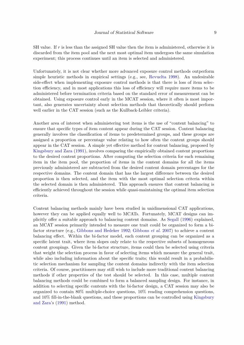
Unfortunately, it is not clear whether more advanced exposure control methods outperformsimple heuristic methods in empirical settings (e.g., see, Revuelta 1998). An undesirableside-effect when implementing exposure control methods is that there is loss of item selec-tion efficiency, and in most applications this loss of efficiency will require more items to beadministered before termination criteria based on the standard error of measurement can beobtained. Using exposure control early in the MCAT session, where it often is most impor-tant, also generates uncertainty about selection methods that theoretically should performwell earlier in the CAT session (such as the Kullback-Leibler criteria).
Another area of interest when administering test items is the use of “content balancing” toensure that specific types of item content appear during the CAT session. Content balancinggenerally involves the classification of items to predetermined groups, and these groups areassigned a proportion or percentage value relating to how often the content groups shouldappear in the CAT session. A simple yet effective method for content balancing, proposed byKingsbury and Zara (1991), involves comparing the empirically obtained content proportionsto the desired content proportions. After computing the selection criteria for each remainingitem in the item pool, the proportion of items in the content domains for all the itemspreviously administered are subtracted from the desired content domain percentages for therespective domains. The content domain that has the largest difference between the desiredproportion is then selected, and the item with the most optimal selection criteria withinthe selected domain is then administered. This approach ensures that content balancing isefficiently achieved throughout the session while quasi-maintaining the optimal item selectioncriteria.
Content balancing methods mainly have been studied in unidimensional CAT applications,however they can be applied equally well to MCATs. Fortunately, MCAT designs can im-plicitly offer a suitable approach to balancing content domains. As Segall (1996) explained,an MCAT session primarily intended to measure one trait could be organized to form a bi-factor structure (e.g., Gibbons and Hedeker 1992; Gibbons et al. 2007) to achieve a contentbalancing effect. Within the bi-factor model, each content grouping can be organized as aspecific latent trait, where item slopes only relate to the respective subsets of homogeneouscontent groupings. Given the bi-factor structure, items could then be selected using criteriathat weight the selection process in favor of selecting items which measure the general trait,while also including information about the specific traits; this would result in a probabilis-tic selection mechanism for sampling the content domains indirectly with the item selectioncriteria. Of course, practitioners may still wish to include more traditional content balancingmethods if other properties of the test should be selected. In this case, multiple contentbalancing methods could be combined to form a balanced sampling design. For instance, inaddition to selecting specific contents with the bi-factor design, a CAT session may also beorganized to contain 80% multiple-choice questions, 10% reading comprehension questions,and 10% fill-in-the-blank questions, and these proportions can be controlled using Kingsburyand Zara’s (1991) method.
10 Generating CAT Interfaces for MIRT Applications
2.4. Termination criteria
In the interest of time, item bank security, and avoiding fatigue effects, one or more stoppingcriteria should be included in MCATs. One reasonable approach to terminating the MCATapplication is to require all SE(θ̂k) ≤ δ, where δ is a maximally tolerable standard error ofmeasurement for all the latent traits. However, if some elements in θ̂ should be measuredwith more precision then unique δk values for each θ̂k value should be defined. For example,if the MCAT is organized to contain a bi-factor structure then the test developer may wish toterminate the session when only the primary trait reaches a predefined δk value. Unequal δkvalues should be used in conjunction with the W-rule, weighted T-rule, or weighted A-rule, sothat items which accurately measure the traits of interest are selected with greater frequency.Classification-based criteria also exist for terminating MCATs when cutoff values are suppliedfor each trait. In classification-based MCATs, the session may be terminated when the confi-dence intervals (given 1− α) for each θ̂ do not contain the pre-specified cutoff values. Whenthe CI (θ̂)s do not contain the cutoff values then the individuals may be classified as above orbelow the cutoff values for the respective traits, otherwise the MCAT results will suggest thatnot enough information exists to reject the plausibility of the cutoffs. More specific methodsfor terminating CATs are also possible (e.g., use of loss functions or risk analyses), howeverthese are not explored in this article.Finally, termination criteria can be based on other practical considerations as well, such assetting the maximum number of items that can be administered in a given session, stoppingthe CAT after a specific amount of time has elapsed, the θ̂ values are changing very little asnew items are added, and so on.
3. The mirtCAT packageThe mirtCAT package (available from the Comprehensive R Archive Network at https://CRAN.R-project.org/package=mirtCAT) provides tools for test developers to generateGUIs for CATs as well as functions for Monte Carlo simulation studies involving CAT de-signs. mirtCAT uses the HTML generating tools available in the shiny package (RStudioInc. 2014) to generate real-time CATs for interactive sessions within standard web-browsingsoftware. The mirtCAT package builds and extends upon the estimation tools available inthe mirt package (Chalmers 2012), and provides a wide range of support for any mixture ofunidimensional and multidimensional IRT models to be used for CATs.Currently supported models in mirtCAT include unidimensional and multidimensional ver-sions of the 4PL model (Lord 1980), the graded response model and its rating scale coun-terpart (Muraki 1992; Muraki and Carlson 1995; Samejima 1969), the generalized partialcredit and nominal model (Thissen et al. 2010), the partially compensatory model (Chalmersand Flora 2014; Sympson 1977), the nested-logit model (Suh and Bolt 2010), the ideal-point model (Maydeu-Olivares, Hernández, and McDonald 2006), and polynomial or productconstructed latent trait combinations (Bock and Aitkin 1981). Additionally, the mirt pack-age supports the use of prior parameter distributions, linear and non-linear parameter con-straints (e.g., see, Chalmers 2015), and specification of fixed parameter values; hence, nestedversions of the previously mentioned models can be estimated from empirical data. For in-stance, the 1PL model (Thissen 1982) can be formed in mirt because it is a highly nestedversion of the M4PL model with equality constraints for the slope parameters.
Journal of Statistical Software 11
3.1. A simple non-adaptive GUI exampleThe mirtCAT package generates interactive GUIs to run CATs by providing inputs to themirtCAT() function. When generating a GUI, the mirtCAT() function requires a data.frameobject containing questions, response options, and output types. When only a data.frameis supplied, a non-adaptive test (i.e., a survey) will be initialized because no IRT parameterswere defined for selecting the items adaptively.Currently, the required inputs names in the data.frame object are:
• Question – A character vector containing all the question stems.
• Option.# – Possible response options for each item, where # corresponds to the specificcategory. For instance, a test with 4 unique response options for each item would containthe columns “Option.1”, “Option.2”, “Option.3”, and “Option.4”. If some items havefewer categories than others then NA placeholders must be used to omit the unusedoptions.
• Type – Indicates the type of response input to use from the shiny package. The sup-ported types are: "radio" for radio buttons, "select" for a pull-down box for selectinginputs, "text" for requiring typed user input, "checkbox" for collecting multiple check-boxes of responses for each item, "slider" for slider-style inputs, and "none" when onlyan item stem should be presented.
• Answer or Answer.# – (Optional) A character vector (or multiple character vectors)indicating the scoring key for items that have correct answers. If there is no correct an-swer for a question then NA values must be specified as placeholders. When a checkboxtype is used with this input then responses are scored according to how many matcheswere selected.
• Stem – (Optional) A character vector of absolute or relative paths pointing to externalmarkdown (.md) or HTML (.html) files, which can be used as item stems. NAs are usedif the item has no corresponding file.
• ... – Additional optional argument inputs that are passed to the associated shinyconstruction functions. For the "slider" input, however, a column for the "min","max", and "step" arguments must be defined.
When generating surveys with mirtCAT, only the Type, Question, and Option inputs aretypically required. If questions are to be scored in real time (as they generally are in abilitymeasuring CATs) then a suitable Answer vector must be supplied. Finally, if specific graphicalstimuli should be included then the paths pointing to the item-stem files must be included inthe Stem input.Before generating a real-time CAT GUI, it is informative to first generate a simple survey tohighlight the fundamental mirtCAT() inputs. For example, say that a researcher wishes tobuild a small survey with only three rating scale items, where each item contains five rating-scale options ranging from “Strongly Disagree” to “Strongly Agree”. Initializing the HTMLinterface to collect responses can be accomplished with the following code:
R> library("mirtCAT")R> options <- matrix(c("Strongly Disagree", "Disagree", "Neutral",
12 Generating CAT Interfaces for MIRT Applications
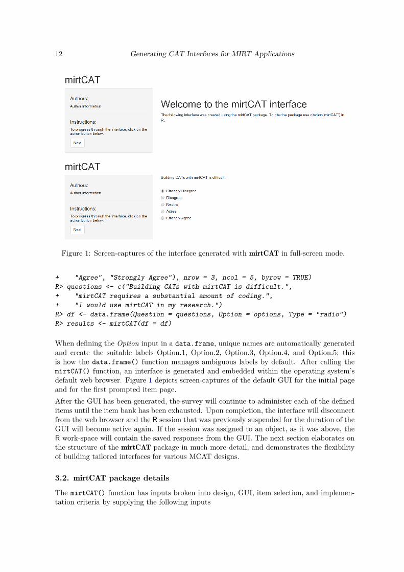
Figure 1: Screen-captures of the interface generated with mirtCAT in full-screen mode.
+ "Agree", "Strongly Agree"), nrow = 3, ncol = 5, byrow = TRUE)R> questions <- c("Building CATs with mirtCAT is difficult.",+ "mirtCAT requires a substantial amount of coding.",+ "I would use mirtCAT in my research.")R> df <- data.frame(Question = questions, Option = options, Type = "radio")R> results <- mirtCAT(df = df)
When defining the Option input in a data.frame, unique names are automatically generatedand create the suitable labels Option.1, Option.2, Option.3, Option.4, and Option.5; thisis how the data.frame() function manages ambiguous labels by default. After calling themirtCAT() function, an interface is generated and embedded within the operating system’sdefault web browser. Figure 1 depicts screen-captures of the default GUI for the initial pageand for the first prompted item page.After the GUI has been generated, the survey will continue to administer each of the defineditems until the item bank has been exhausted. Upon completion, the interface will disconnectfrom the web browser and the R session that was previously suspended for the duration of theGUI will become active again. If the session was assigned to an object, as it was above, theR work-space will contain the saved responses from the GUI. The next section elaborates onthe structure of the mirtCAT package in much more detail, and demonstrates the flexibilityof building tailored interfaces for various MCAT designs.
3.2. mirtCAT package details
The mirtCAT() function has inputs broken into design, GUI, item selection, and implemen-tation criteria by supplying the following inputs
Journal of Statistical Software 13
Arguments Description Possible inputsdf Named data.frame containing
questions, options, answers, outputtypes, and graphical stem locations.
data.frame or missing.
mo Single group object defined by the mirtpackage. This is required if the test isto be scored.
Object of class SingleGroupClassor missing.
method Character string for selecting themethod of predicting θ̂ values.
"MAP", "EAP", "ML", "WLE","EAPsum", "fixed"
criteria Adaptive and non-adaptive itemselection criteria to be used. Someinputs are available exclusively forunidimensional or multidimensionaltests.
"seq", "random", "MI", "MEPV","MLWI", "MPWI", "MEI", "IKL","IKLP", "IKLn", "IKLPn","Drule", "DPrule", "Erule","EPrule", "Trule", "TPrule","Arule", "APrule", "Wrule","WPrule", "KL", "KLn"
start_item Numeric value or character stringindicating which item is to beadministered first. Default is 1 toadminister the first item in the test. Ifa suitable character string is suppliedinstead, the initial item will be selectedfrom the options available in criteria.
Numeric scalar or character string.
local_pattern If df was supplied, a character matrix(with one row) specifying how aparticipant responded to the test,otherwise an integer matrix (withpotentially more than one row). Ifsupplied, the GUI will not be generatedand instead the MCAT results will beevaluated off-line.
Character or integer matrix.
design_elements A logical value indicating whether a listcontaining the design objects should bereturned.
Logical scalar.
cl An optional cluster object defined withthe parallel package. Used forsimulation designs that should be runin parallel.
Cluster object defined byparallel::makeCluster().
... Additional arguments to be passed tofunction such as mirt::fscores().
–
Table 1: Selection of inputs for mirtCAT().
mirtCAT(df, mo, method = "MAP", criteria = "seq", start_item = 1,local_pattern = NULL, design_elements = FALSE, cl = NULL,design = list(), shinyGUI = list(), preCAT = list(), ...)
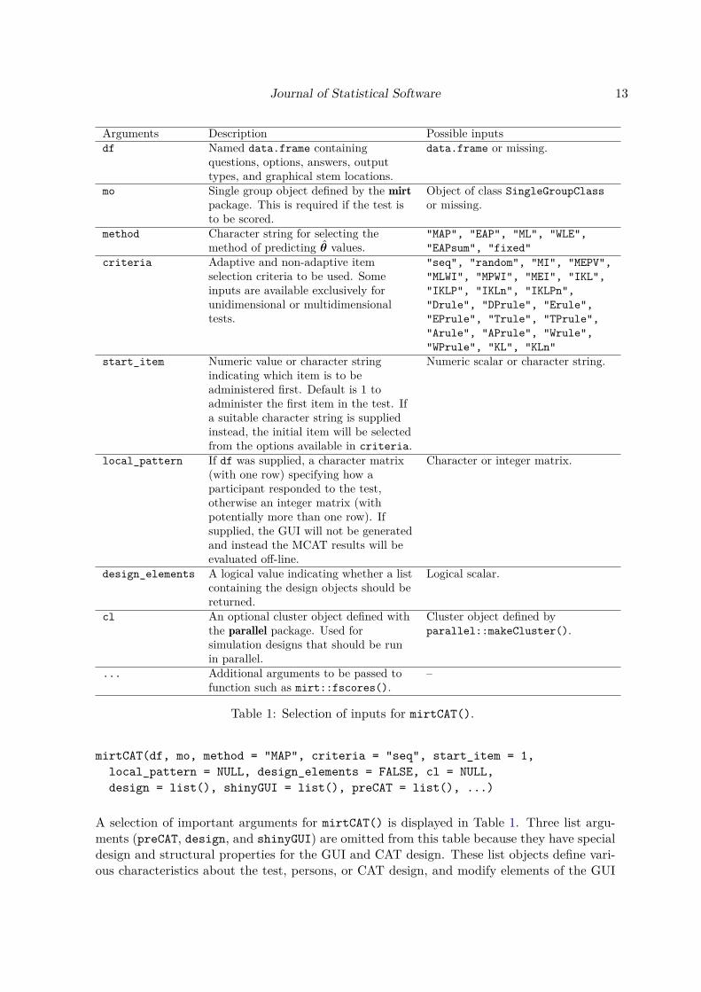
A selection of important arguments for mirtCAT() is displayed in Table 1. Three list argu-ments (preCAT, design, and shinyGUI) are omitted from this table because they have specialdesign and structural properties for the GUI and CAT design. These list objects define vari-ous characteristics about the test, persons, or CAT design, and modify elements of the GUI
14 Generating CAT Interfaces for MIRT Applications
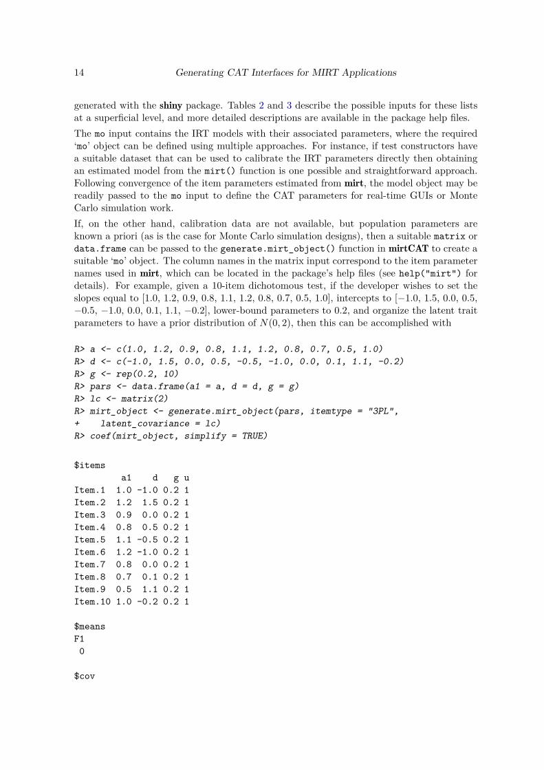
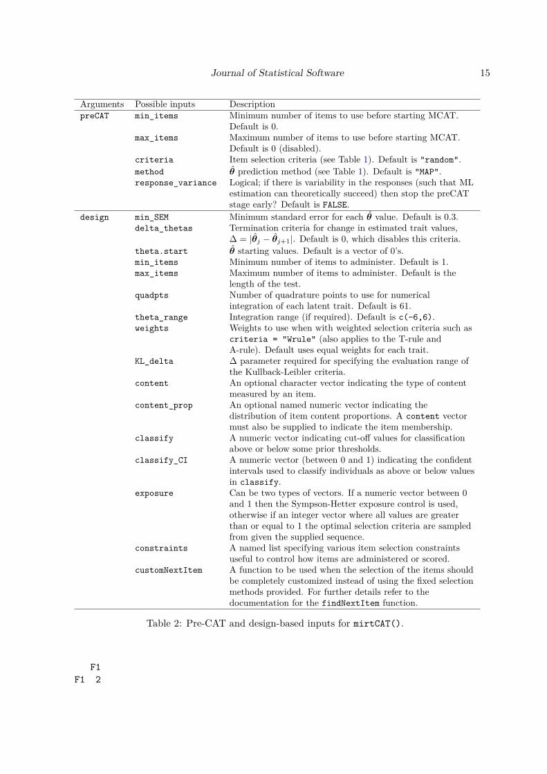
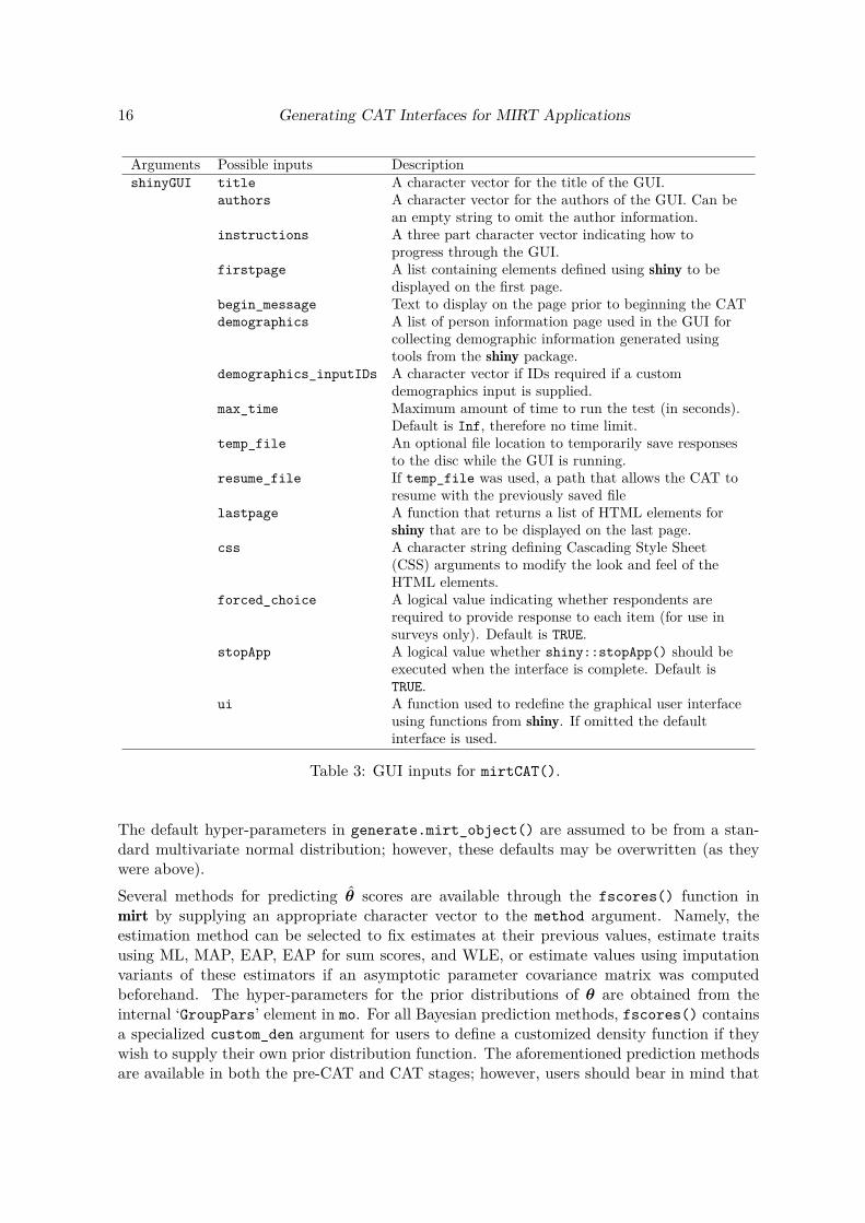
generated with the shiny package. Tables 2 and 3 describe the possible inputs for these listsat a superficial level, and more detailed descriptions are available in the package help files.The mo input contains the IRT models with their associated parameters, where the required‘mo’ object can be defined using multiple approaches. For instance, if test constructors havea suitable dataset that can be used to calibrate the IRT parameters directly then obtainingan estimated model from the mirt() function is one possible and straightforward approach.Following convergence of the item parameters estimated from mirt, the model object may bereadily passed to the mo input to define the CAT parameters for real-time GUIs or MonteCarlo simulation work.If, on the other hand, calibration data are not available, but population parameters areknown a priori (as is the case for Monte Carlo simulation designs), then a suitable matrix ordata.frame can be passed to the generate.mirt_object() function in mirtCAT to create asuitable ‘mo’ object. The column names in the matrix input correspond to the item parameternames used in mirt, which can be located in the package’s help files (see help("mirt") fordetails). For example, given a 10-item dichotomous test, if the developer wishes to set theslopes equal to [1.0, 1.2, 0.9, 0.8, 1.1, 1.2, 0.8, 0.7, 0.5, 1.0], intercepts to [−1.0, 1.5, 0.0, 0.5,−0.5, −1.0, 0.0, 0.1, 1.1, −0.2], lower-bound parameters to 0.2, and organize the latent traitparameters to have a prior distribution of N(0, 2), then this can be accomplished with
R> a <- c(1.0, 1.2, 0.9, 0.8, 1.1, 1.2, 0.8, 0.7, 0.5, 1.0)R> d <- c(-1.0, 1.5, 0.0, 0.5, -0.5, -1.0, 0.0, 0.1, 1.1, -0.2)R> g <- rep(0.2, 10)R> pars <- data.frame(a1 = a, d = d, g = g)R> lc <- matrix(2)R> mirt_object <- generate.mirt_object(pars, itemtype = "3PL",+ latent_covariance = lc)R> coef(mirt_object, simplify = TRUE)
$itemsa1 d g u
Item.1 1.0 -1.0 0.2 1Item.2 1.2 1.5 0.2 1Item.3 0.9 0.0 0.2 1Item.4 0.8 0.5 0.2 1Item.5 1.1 -0.5 0.2 1Item.6 1.2 -1.0 0.2 1Item.7 0.8 0.0 0.2 1Item.8 0.7 0.1 0.2 1Item.9 0.5 1.1 0.2 1Item.10 1.0 -0.2 0.2 1
$meansF10
$cov
Journal of Statistical Software 15
Arguments Possible inputs DescriptionpreCAT min_items Minimum number of items to use before starting MCAT.
Default is 0.max_items Maximum number of items to use before starting MCAT.
Default is 0 (disabled).criteria Item selection criteria (see Table 1). Default is "random".method θ̂ prediction method (see Table 1). Default is "MAP".response_variance Logical; if there is variability in the responses (such that ML
estimation can theoretically succeed) then stop the preCATstage early? Default is FALSE.
design min_SEM Minimum standard error for each θ̂ value. Default is 0.3.delta_thetas Termination criteria for change in estimated trait values,
∆ = |θ̂j − θ̂j+1|. Default is 0, which disables this criteria.theta.start θ̂ starting values. Default is a vector of 0’s.min_items Minimum number of items to administer. Default is 1.max_items Maximum number of items to administer. Default is the
length of the test.quadpts Number of quadrature points to use for numerical
integration of each latent trait. Default is 61.theta_range Integration range (if required). Default is c(-6,6).weights Weights to use when with weighted selection criteria such as
criteria = "Wrule" (also applies to the T-rule andA-rule). Default uses equal weights for each trait.
KL_delta ∆ parameter required for specifying the evaluation range ofthe Kullback-Leibler criteria.
content An optional character vector indicating the type of contentmeasured by an item.
content_prop An optional named numeric vector indicating thedistribution of item content proportions. A content vectormust also be supplied to indicate the item membership.
classify A numeric vector indicating cut-off values for classificationabove or below some prior thresholds.
classify_CI A numeric vector (between 0 and 1) indicating the confidentintervals used to classify individuals as above or below valuesin classify.
exposure Can be two types of vectors. If a numeric vector between 0and 1 then the Sympson-Hetter exposure control is used,otherwise if an integer vector where all values are greaterthan or equal to 1 the optimal selection criteria are sampledfrom given the supplied sequence.
constraints A named list specifying various item selection constraintsuseful to control how items are administered or scored.
customNextItem A function to be used when the selection of the items shouldbe completely customized instead of using the fixed selectionmethods provided. For further details refer to thedocumentation for the findNextItem function.
Table 2: Pre-CAT and design-based inputs for mirtCAT().
F1F1 2
16 Generating CAT Interfaces for MIRT Applications
Arguments Possible inputs DescriptionshinyGUI title A character vector for the title of the GUI.
authors A character vector for the authors of the GUI. Can bean empty string to omit the author information.
instructions A three part character vector indicating how toprogress through the GUI.
firstpage A list containing elements defined using shiny to bedisplayed on the first page.
begin_message Text to display on the page prior to beginning the CATdemographics A list of person information page used in the GUI for
collecting demographic information generated usingtools from the shiny package.
demographics_inputIDs A character vector if IDs required if a customdemographics input is supplied.
max_time Maximum amount of time to run the test (in seconds).Default is Inf, therefore no time limit.
temp_file An optional file location to temporarily save responsesto the disc while the GUI is running.
resume_file If temp_file was used, a path that allows the CAT toresume with the previously saved file
lastpage A function that returns a list of HTML elements forshiny that are to be displayed on the last page.
css A character string defining Cascading Style Sheet(CSS) arguments to modify the look and feel of theHTML elements.
forced_choice A logical value indicating whether respondents arerequired to provide response to each item (for use insurveys only). Default is TRUE.
stopApp A logical value whether shiny::stopApp() should beexecuted when the interface is complete. Default isTRUE.
ui A function used to redefine the graphical user interfaceusing functions from shiny. If omitted the defaultinterface is used.
Table 3: GUI inputs for mirtCAT().
The default hyper-parameters in generate.mirt_object() are assumed to be from a stan-dard multivariate normal distribution; however, these defaults may be overwritten (as theywere above).Several methods for predicting θ̂ scores are available through the fscores() function inmirt by supplying an appropriate character vector to the method argument. Namely, theestimation method can be selected to fix estimates at their previous values, estimate traitsusing ML, MAP, EAP, EAP for sum scores, and WLE, or estimate values using imputationvariants of these estimators if an asymptotic parameter covariance matrix was computedbeforehand. The hyper-parameters for the prior distributions of θ are obtained from theinternal ‘GroupPars’ element in mo. For all Bayesian prediction methods, fscores() containsa specialized custom_den argument for users to define a customized density function if theywish to supply their own prior distribution function. The aforementioned prediction methodsare available in both the pre-CAT and CAT stages; however, users should bear in mind that
Journal of Statistical Software 17
methods which can handle extreme response patterns (such as MAP) may be beneficial inthe pre-CAT stage.There are multiple item selection criteria available in mirtCAT, some of which are onlyapplicable to unidimensional or multidimensional models. Criteria applicable to both uni-dimensional and multidimensional adaptive tests are the "KL" and "KLn" method for thepoint-wise Kullback-Leibler divergence and the point-wise Kullback-Leibler with a decreasingdelta value (∆ ·
√n, where n is the number of items previous answered), respectively, "IKLP"
and "IKL" for the integration based Kullback-Leibler criteria with and without the prior den-sity weight, and "IKLn" and "IKLPn" for the
√n sequentially weighted counter-parts of the
integration criteria (Chang and Ying 1996). Possible inputs for unidimensional adaptive testsinclude "MI" for the maximum information criteria, "MEPV" for minimum expected posteriorvariance, "MLWI" for maximum-likelihood with weighted information, "MPWI" for maximumposterior weighted information, and "MEI" for maximum expected information (see Magisand Raîche 2012, and the references therein for further elaboration of these methods).Possible inputs for multidimensional adaptive tests include the "Drule" for the maximumdeterminant of the information matrix, "Trule" for the maximum (weighted) trace of theinformation matrix, "Arule" for the minimum (weighted) trace of the asymptotic covariancematrix, "Erule" for the minimum eigenvalue of the information matrix, and "Wrule" for theweighted information criteria. The multivariate selection criteria have posterior weighted ana-logues for Bayesian selection, which are available by passing "DPrule", "TPrule", "EPrule",and "WPrule", where the “P” indicates the use of a prior distribution. Finally, non-adaptiveselection methods include the sequential ("seq" ) and random ("random") criteria, which canbe used in both adaptive and non-adaptive tests.
3.3. Auxiliary functionsUpon completion of the mirtCAT() function, an S3 object of class ‘mirtCAT’ is returnedand contains information about the raw and scored response pattern, person demographicssupplied in the survey, order in which the items were administered, estimation history, andfinal trait estimates. Three generic S3 methods, print(), summary(), and plot(), have beendefined to help summarize the returned object. The print() method will display the numberof items administered and, if mirtCAT() was supplied suitable item parameters, the final θ̂and SE(θ̂) estimates. summary() will return a list of more detailed information about the rawand scored response patterns, items administered, item response times (in seconds), historyof the θ̂ and SE(θ̂) estimates, and so on. Finally, plot() will generate figures based onthe estimation history of θ̂ and SE(θ̂) (or confidence intervals) to display how the test wasprogressively scored.When constructing CATs, developers may wish to experiment with their CAT designs bysupplying fixed response patterns. mirtCAT eases the construction of plausible responsepatterns through the generate_pattern() function, and allows the CAT interface to berun without generating a GUI by passing an object containing suitable response patterns tomirtCAT(..., local_pattern). For example, a participant with a latent ability score ofθ = 1 could create the following response pattern.
R> set.seed(1)R> pattern <- generate_pattern(mirt_object, Theta = 1)R> pattern

18 Generating CAT Interfaces for MIRT Applications
[,1] [,2] [,3] [,4] [,5] [,6] [,7] [,8] [,9] [,10][1,] 0 1 1 1 0 1 1 1 1 0
The generate_pattern() function sequentially generates plausible responses for each item inthe item pool, and stores these values into a matrix. If generate_pattern() were supplied thedf object with the respective item options then the function would return a character matrixof plausible responses instead of an integer matrix. The Theta input to generate_pattern()can be either a numeric vector to generate a single response pattern or a matrix of latenttrait values to generate a matrix of plausible patterns corresponding to the rows in Theta.Supplying a matrix of trait values is especially useful for generating plausible response patternsfor Monte Carlo simulation work, as we will observe in Section 5.After generating one or more response patterns, the matrix is then passed to the local_patternargument to execute the CAT session(s) off-line. As a simple example of how one might usethese response patterns, the following CAT was designed to select all items with the maximuminformation ("MI") selection criteria.
R> result <- mirtCAT(mo = mirt_object, local_pattern = pattern,+ start_item = "MI", criteria = "MI")R> print(result)
n.items.answered Theta_1 SE.Theta_110 0.3355295 0.7412856
R> summary(result)
$final_estimatesTheta_1
Estimates 0.3355295SEs 0.7412856
$raw_responses[1] "1" "2" "1" "2" "2" "2" "1" "2" "2" "2"
$scored_responses[1] 0 1 0 1 1 1 0 1 1 1
$items_answered[1] 5 2 10 3 4 6 1 7 8 9
$thetas_historyTheta_1
[1,] 0.000000000[2,] -0.548189757[3,] -0.263133573[4,] -0.596607706[5,] -0.315643850
Journal of Statistical Software 19
CAT Standard Errors
Item
θ
−1.5
−1.0
−0.5
0.0
0.5
1.0
0 5 2 10 3 4 6 1 7 8 9
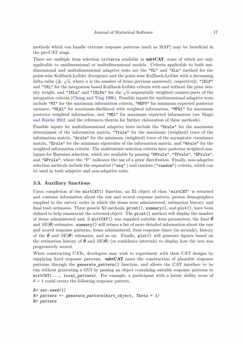
Figure 2: Output of plot() method for ‘mirtCAT’ objects.
[6,] -0.134086560[7,] 0.201131905[8,] 0.002223685[9,] 0.165947607
[10,] 0.288851261[11,] 0.335529460
$thetas_SE_historyTheta_1
[1,] 1.4142136[2,] 1.1733174[3,] 1.0314490[4,] 0.9390705[5,] 0.8992738[6,] 0.8600807[7,] 0.8499782[8,] 0.8114719[9,] 0.7753160
[10,] 0.7507978[11,] 0.7412856
R> plot(result)
The plot is shown in Figure 2.Administering an adaptive test using an item bank with only 10-items clearly is not optimalfor accurately measuring θ = 1, however this example is only intended to demonstrate how
20 Generating CAT Interfaces for MIRT Applications
the output is summarized. After calling the summary(result) function, a list containingvarious CAT elements is returned. The $items_answered and $scored_responses elementstogether indicate that item five was answered first with scored response 1, followed by itemsix with a scored response of 0, then item ten with a scored response of 1, and so on un-til item nine was chosen last by default with a scored response of 1. The $raw_responseselement from the summary() output indicates which category was selected in the GUI orsimulated response pattern; for off-line analyses this element can largely be ignored and sim-ply indicates placeholder categories. The corresponding θ̂ and SE(θ̂) estimates are shownin the $thetas_history and $thetas_SE_history elements, and demonstrate how the abil-ity estimates, and their respective standard errors, successively change after each item isadministered.At this point is useful to note the connection with mirt, which thus far has silently per-formed all the computations of the θ̂ and SE(θ̂) estimates. The list of outputs returnedby summary(result, sort = FALSE) can readily be used by functions in the mirt pack-age by selecting various elements from the list output. More specifically, the unsorted$scored_responses element can be added to a calibration dataset (if the parameters werepreviously estimated) by simple use of the rbind() function. Including new response data tothe original calibration dataset can be useful when recalibrating the parameter estimates ata later time. Additionally, the unsorted response pattern could be passed into fscores(...,response.pattern = pattern) to further examine what the θ̂ would have been given alter-native prediction methods. For instance, if the above response pattern were to be estimatedwith the ML prediction method then the estimates would be
R> responses <- summary(result, sort = FALSE)$scored_responsesR> fscores(mirt_object, response.pattern = responses, method = "ML")
Item.1 Item.2 Item.3 Item.4 Item.5 Item.6 Item.7 Item.8 Item.9[1,] 0 1 1 1 0 1 1 1 1
Item.10 F1 SE_F1[1,] 0 0.4609681 0.8596507
Because all items were administered, the unsorted response pattern is identical to the patterngenerated from generate_pattern(). If items were not responded to due to early terminationof the CAT then NA values would be present in the items containing no observations.
4. Single case MCAT exampleIn this section, an MCAT design and graphical user interface are constructed using the codelocated in Appendix A. The questions and item parameters were arranged to emulate how amultidimensional mathematical achievement test with cross-factor loadings and correlated la-tent traits could be managed. The item bank consisted of 120 items in total, and a data.frameobject with the questions and answers was included. The first 30 items were constructed tomeasure only a hypothetical “Addition” trait, while the last 30 items measured only on a“Multiplication” trait. The middle 60 items were evenly split to contain a mix of the Addi-tion and Multiplication slopes. However, the first half of these items were designed to relatemore to the Addition trait (contained larger slopes), while the last 30 items were designed to
Journal of Statistical Software 21
Test Information
−3−2
−10
12
3
−3
−2
−1
0
12
3
10
20
30
40
θ1
θ2
I(θ)
5
10
15
20
25
30
35
40
45
Test Standard Errors
−3−2
−10
12
3
−3
−2
−1
0
12
3
0.20
0.25
0.30
0.35
0.40
θ1
θ2
SE(θ)
0.15
0.20
0.25
0.30
0.35
0.40
0.45
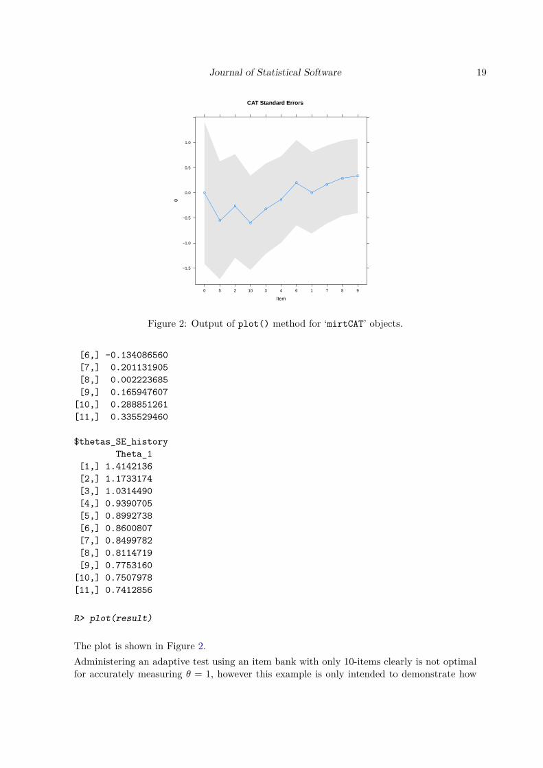
Figure 3: Plots of test implied response functions from models estimated in the mirt package.
relate more to the Multiplication trait. The expected information and standard error plotsbelow indicate that respondents with abilities closer to the center of the distributions will bemeasured with the most accuracy, while those in the more extreme ends of the ability rangewill be measured with much less precision.
R> plot(mod, type = "info", theta_lim = c(-3, 3))R> plot(mod, type = "SE", theta_lim = c(-3, 3))
The resulting plots are shown in Figure 3.Given the objects defined in Appendix A, we first generate a plausible observed responsepattern for a participant with abilities θ = [−0.5, 0.5].
R> set.seed(1)R> pat <- generate_pattern(mo = mod, Theta = c(-0.5, 0.5), df = df)R> head(pat)
[1] "145" "195" "200" "232" "207" "175"
The character responses indicates that, among the options in df[1, ], the category pertainingto the option "145" was selected as the correct answer, "195" was selected for the seconditem among the possible options in df[2, ], and so on for the remaining 118 items. Todetermine how the MCAT session would behave if each item were administered in sequence,the min_items argument could be increased to ensure that all items are selected; alternatively,the min_SEM input could be decreased to a much smaller value to accomplish the same goal.
R> result <- mirtCAT(df = df, mo = mod, local_pattern = pat,+ design = list(min_items = 120))R> print(result)
22 Generating CAT Interfaces for MIRT Applications
CAT Standard Errors
Item
θ
−1.0
−0.5
0.0
0.5
1.0
●
●
●
●
●
●
●
●
●
●
●
●
●
●
●●
●
●
●
●
●
●
●
●
●
●●
●●
●●
●
●●
●●
●●
●●
●
●●●
●●
●●●
●●
●●
●●
●●●●
●●●
●●●●●●●●●●●●●●●●●●●●●●●●●●●●●●●●●●●●●●●●●●●●●●●●●●●●●●●●●●●
Theta_1
●●
●
●
●
●
●
●●
●
●●
●●
●●
●●
●
●●
●●
●●
●●●●●●
●
●
●
●●
●
●
●
●
●
●●●
●
●●●●
●●●●
●
●●●●●
●●
●
●
●
●
●
●●
●
●
●
●
●
●
●●
●●●
●
●●
●
●●
●
●
●●
●
●●
●●●●
●●●●
●●
●●●
●●
●●●
●
●●●●●●
●
●●●
Theta_2
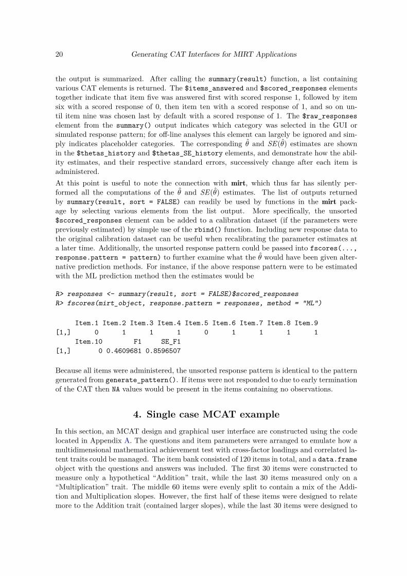
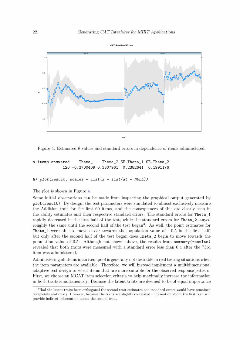
Figure 4: Estimated θ values and standard errors in dependence of items administered.
n.items.answered Theta_1 Theta_2 SE.Theta_1 SE.Theta_2120 -0.3700409 0.3307961 0.2382641 0.1991176
R> plot(result, scales = list(x = list(at = NULL))
The plot is shown in Figure 4.Some initial observations can be made from inspecting the graphical output generated byplot(result). By design, the test parameters were simulated to almost exclusively measurethe Addition trait for the first 60 items, and the consequences of this are clearly seen inthe ability estimates and their respective standard errors. The standard errors for Theta_1rapidly decreased in the first half of the test, while the standard errors for Theta_2 stayedroughly the same until the second half of the test began3. As well, the point estimates forTheta_1 were able to move closer towards the population value of −0.5 in the first half,but only after the second half of the test began does Theta_2 begin to move towards thepopulation value of 0.5. Although not shown above, the results from summary(results)revealed that both traits were measured with a standard error less than 0.4 after the 73rditem was administered.Administering all items in an item pool is generally not desirable in real testing situations whenthe item parameters are available. Therefore, we will instead implement a multidimensionaladaptive test design to select items that are more suitable for the observed response pattern.First, we choose an MCAT item selection criteria to help maximally increase the informationin both traits simultaneously. Because the latent traits are deemed to be of equal importance
3Had the latent traits been orthogonal the second trait estimates and standard errors would have remainedcompletely stationary. However, because the traits are slightly correlated, information about the first trait willprovide indirect information about the second trait.

Journal of Statistical Software 23
in this example, the use of the D-rule for selecting items is a reasonable choice. Next, we setthe stopping criteria for the standard error of measurement to 0.4 for all traits. The responsepattern previously simulated is then reanalyzed in mirtCAT() with
R> set.seed(1234)R> MCATresult <- mirtCAT(df = df, mo = mod, criteria = "Drule",+ local_pattern = pat, start_item = "Drule",+ design = list(min_SEM = 0.4))R> print(MCATresult)
n.items.answered Theta_1 Theta_2 SE.Theta_1 SE.Theta_218 -0.5315822 0.7334699 0.3922312 0.3525484
R> summary(MCATresult)
$final_estimatesTheta_1 Theta_2
Estimates -0.5315822 0.7334699SEs 0.3922312 0.3525484
$raw_responses[1] "3" "2" "1" "3" "3" "5" "5" "3" "1" "3" "3" "1" "1" "3" "4" "1" "5" "4"
$scored_responses[1] 1 0 0 1 0 1 1 0 1 1 1 1 1 1 0 1 1 0
$items_answered[1] 40 118 59 65 41 3 93 31 87 63 107 24 96 82 5 15 110 21
$thetas_historyTheta_1 Theta_2
[1,] 0.0000000 0.000000000[2,] 0.3300104 0.279113425[3,] 0.1417429 -0.280431989[4,] -0.3095254 -0.381602240[5,] -0.2671319 -0.118300123[6,] -0.6102685 -0.162056553[7,] -0.3903506 -0.144267168[8,] -0.3774346 0.003104662[9,] -0.5382688 -0.006176610
[10,] -0.5065322 0.176070232[11,] -0.4950992 0.384451064[12,] -0.4864141 0.521754123[13,] -0.3538263 0.527263358[14,] -0.3480257 0.626719891[15,] -0.3465018 0.697100900[16,] -0.4941311 0.690762595
24 Generating CAT Interfaces for MIRT Applications
[17,] -0.4398394 0.693084295[18,] -0.4374101 0.737414618[19,] -0.5315822 0.733469944
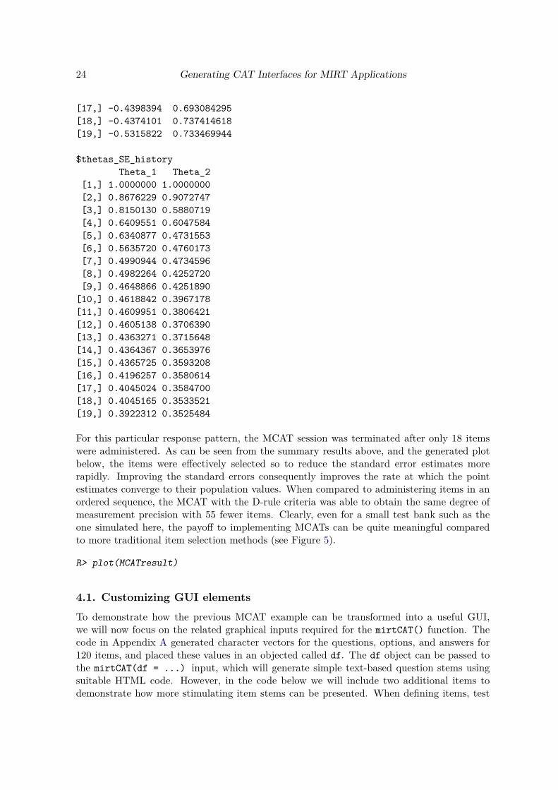
$thetas_SE_historyTheta_1 Theta_2
[1,] 1.0000000 1.0000000[2,] 0.8676229 0.9072747[3,] 0.8150130 0.5880719[4,] 0.6409551 0.6047584[5,] 0.6340877 0.4731553[6,] 0.5635720 0.4760173[7,] 0.4990944 0.4734596[8,] 0.4982264 0.4252720[9,] 0.4648866 0.4251890
[10,] 0.4618842 0.3967178[11,] 0.4609951 0.3806421[12,] 0.4605138 0.3706390[13,] 0.4363271 0.3715648[14,] 0.4364367 0.3653976[15,] 0.4365725 0.3593208[16,] 0.4196257 0.3580614[17,] 0.4045024 0.3584700[18,] 0.4045165 0.3533521[19,] 0.3922312 0.3525484
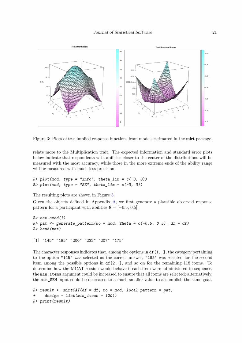
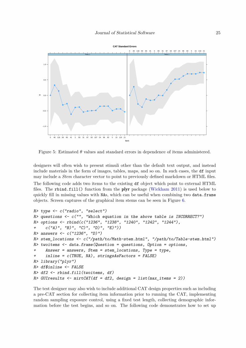
For this particular response pattern, the MCAT session was terminated after only 18 itemswere administered. As can be seen from the summary results above, and the generated plotbelow, the items were effectively selected so to reduce the standard error estimates morerapidly. Improving the standard errors consequently improves the rate at which the pointestimates converge to their population values. When compared to administering items in anordered sequence, the MCAT with the D-rule criteria was able to obtain the same degree ofmeasurement precision with 55 fewer items. Clearly, even for a small test bank such as theone simulated here, the payoff to implementing MCATs can be quite meaningful comparedto more traditional item selection methods (see Figure 5).
R> plot(MCATresult)
4.1. Customizing GUI elements
To demonstrate how the previous MCAT example can be transformed into a useful GUI,we will now focus on the related graphical inputs required for the mirtCAT() function. Thecode in Appendix A generated character vectors for the questions, options, and answers for120 items, and placed these values in an objected called df. The df object can be passed tothe mirtCAT(df = ...) input, which will generate simple text-based question stems usingsuitable HTML code. However, in the code below we will include two additional items todemonstrate how more stimulating item stems can be presented. When defining items, test
Journal of Statistical Software 25
CAT Standard Errors
Item
θ
−1.0
−0.5
0.0
0.5
1.0
0 40 118 59 65 41 3 93 31 87 63 107 24 96 82 5 15 110 21
●
●
●
●●
●
● ●
●● ● ●
● ● ●
●
● ●
●
Theta_1
0 40 118 59 65 41 3 93 31 87 63 107 24 96 82 5 15 110 21
●
●
●
●
●● ●
● ●
●
●
● ●
●
● ● ●● ●
Theta_2
Figure 5: Estimated θ values and standard errors in dependence of items administered.
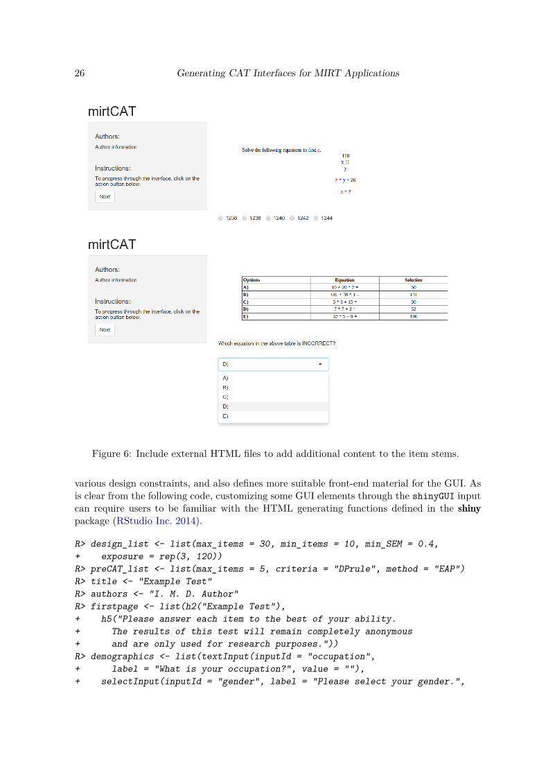
designers will often wish to present stimuli other than the default text output, and insteadinclude materials in the form of images, tables, maps, and so on. In such cases, the df inputmay include a Stem character vector to point to previously defined markdown or HTML files.The following code adds two items to the existing df object which point to external HTMLfiles. The rbind.fill() function from the plyr package (Wickham 2011) is used below toquickly fill in missing values with NAs, which can be useful when combining two data.frameobjects. Screen captures of the graphical item stems can be seen in Figure 6.
R> type <- c("radio", "select")R> questions <- c("", "Which equation in the above table is INCORRECT?")R> options <- rbind(c("1236", "1238", "1240", "1242", "1244"),+ c("A)", "B)", "C)", "D)", "E)"))R> answers <- c("1236", "D)")R> stem_locations <- c("/path/to/Math-stem.html", "/path/to/Table-stem.html")R> twoitems <- data.frame(Question = questions, Option = options,+ Answer = answers, Stem = stem_locations, Type = type,+ inline = c(TRUE, NA), stringsAsFactors = FALSE)R> library("plyr")R> df$inline <- FALSER> df2 <- rbind.fill(twoitems, df)R> GUIresults <- mirtCAT(df = df2, design = list(max_items = 2))
The test designer may also wish to include additional CAT design properties such as includinga pre-CAT section for collecting item information prior to running the CAT, implementingrandom sampling exposure control, using a fixed test length, collecting demographic infor-mation before the test begins, and so on. The following code demonstrates how to set up
26 Generating CAT Interfaces for MIRT Applications
Figure 6: Include external HTML files to add additional content to the item stems.
various design constraints, and also defines more suitable front-end material for the GUI. Asis clear from the following code, customizing some GUI elements through the shinyGUI inputcan require users to be familiar with the HTML generating functions defined in the shinypackage (RStudio Inc. 2014).
R> design_list <- list(max_items = 30, min_items = 10, min_SEM = 0.4,+ exposure = rep(3, 120))R> preCAT_list <- list(max_items = 5, criteria = "DPrule", method = "EAP")R> title <- "Example Test"R> authors <- "I. M. D. Author"R> firstpage <- list(h2("Example Test"),+ h5("Please answer each item to the best of your ability.+ The results of this test will remain completely anonymous+ and are only used for research purposes."))R> demographics <- list(textInput(inputId = "occupation",+ label = "What is your occupation?", value = ""),+ selectInput(inputId = "gender", label = "Please select your gender.",
Journal of Statistical Software 27
+ choices = c("", "Male", "Female", "Other"), selected = ""))R> shinyGUI_list <- list(title = title, authors = authors,+ demographics = demographics,+ demographics_inputIDs = c("occupation", "gender"),+ firstpage = firstpage)R> GUIresults <- mirtCAT(df = df, mo = mod, criteria = "Drule",+ start_item = "DPrule", shinyGUI = shinyGUI_list,+ design = design_list, preCAT = preCAT_list)
The above MCAT design begins with a pre-CAT stage where a total of five items are selectedusing the Bayesian D-rule criteria, while the traits are updated using the EAP method. Next,the MCAT begins, and items are selected according to the D-rule criteria. However, insteadof selecting the most optimal D-rules in both stages, the top three most optimal items arerandomly sampled to determine which item is to be administered next4. The total number ofitems administered are required to be between 10 and 30; however, the test may be terminatedearly if the standard errors for the traits are both less than 0.4. With respect to the GUIpresentation, simple elements such as the title and author names are modified using basic Rcode, while the first, last, and demographic pages were customized using HTML generatingfunctions from the shiny package.
5. Monte Carlo simulationsIn this section, functions in the mirtCAT package for generating Monte Carlo simulationstudies are presented, and the results are compared to existing R packages capable of analyzingCAT designs. The first simulation generates a unidimensional CAT design, and compares theresults from mirtCAT to the catIrt and catR packages (version 0.5-0 and 3.4, respectively).The second design generates a two-dimensional MCAT design, but now compares the resultsto the MAT package (version 2.2). Finally, a third simulation design was constructed usingmirtCAT to generate an MCAT design with mixed-item types, exposure control, contentbalancing, and a weighted item selection criterion.
5.1. Unidimensional simulation design
A unidimensional item bank was constructed to contain 1000 3PL item response models.The item slope parameters were drawn from a log-normal distribution, a ∼ logN(0.2, 0.3),the intercept parameters were drawn from a standard normal distribution, d ∼ N(0, 1), thelower-bound parameters were all set to a constant, g = 0.2, the latent trait values weredrawn from a standard normal distribution, and N = 5000 plausible response patterns weregenerated given the latent trait values and item parameters. Using the mirtCAT package,the plausible response patterns were generated using the following code:
R> nitems <- 1000R> N <- 5000R> Theta <- matrix(rnorm(N))R> a <- matrix(rlnorm(nitems, 0.2, 0.3), nitems)
4When the random sampling exposure control method draws a constant number of options throughout theCAT session this is known as the randomesque method (Kingsbury and Zara 1989).
28 Generating CAT Interfaces for MIRT Applications
R> d <- rnorm(nitems)R> pars <- data.frame(a1 = a, d = d, g = 0.2)R> mirt_object <- generate.mirt_object(pars, "3PL")R> responses <- generate_pattern(mirt_object, Theta = Theta)
Analyzing the matrix of response patterns requires passing the object to the local_patternargument in mirtCAT(). To allow for comparisons between existent R packages, a compatibleCAT design was constructed. The design was organized such that all items were selected usingthe maximum-information criteria (including the initial item), the θ̂ values were updated usingEAP estimation given a standard normal prior, the number of items selected were requiredto be between 10 and 50, and the CAT was terminated early if SE(θ̂) < 0.25.When performing Monte Carlo simulation studies, front-end users should consider using multi-core architecture methods. Invoking more than one processor to perform the computationscan potentially reduce the estimation times by a factor proportional to the number of coresavailable. mirtCAT() explicitly supports parallel computing by accepting a cl argument,where cl is a suitable socket-type object to be used by functions in the parallel package.Analyzing the previously defined CAT design for each response pattern, while capitalizing onmulti-core estimation, can be expressed as
R> library("parallel")R> cl <- makeCluster(detectCores())R> design <- list(min_SEM = 0.25, min_items = 10, max_items = 50)R> mirtCAT_results <- mirtCAT(mo = mirt_object, local_pattern = responses,+ start_item = "MI", method = "EAP", criteria = "MI", design = design,+ cl = cl))
The resulting object returned by mirtCAT() is a list containing independent ‘mirtCAT’ objects,where each element corresponds to the respective row in the responses input. These elementscan further be extracted and analyzed using various simulation summary statistics (e.g., bias,root mean-square deviation, correlations, et cetera; see Section 5.3 and the code in Appendix Bfor a more complete example).The unidimensional CAT design and generated response patterns were then analyzed us-ing code from the catIrt and catR packages. mirtCAT was executed twice to compare theeffect of single versus multi-core architecture (eight processors were selected for the multi-core execution using an Intel i7, 3.40GHz processor; Operating system: Ubuntu, version16.04 LTS). All final ability estimates correlated equally well with the generated populationvalues (r ≈ 0.9689), and returned nearly the exact same estimates (r > 0.9999). However,where these packages differed was in the estimation time required to complete the simulation.The catIrt package was the least efficient at estimating this design, requiring 5733 secondsto complete the simulation (approximately 95 minutes), while catR required 1703 seconds(approximately 28 minutes).5 The mirtCAT package, however, required 565 seconds for ex-ecution with single-core architecture (9 minutes and 25 seconds) and only 144 seconds (2minutes and 24 seconds) when using the internally organized multi-core architecture. As isevident from this simulation, multi-core architecture can be highly effective when performingMonte Carlo studies for CATs.
5Note that catR required a for() loop in order to execute the simulated response patterns because thecurrent version does not support multiple response inputs.
Journal of Statistical Software 29
5.2. Multidimensional simulation design
The second simulation compared numerical results to the MAT package for a simple MCATdesign. A relatively large item bank was organized to consist of 1000 M2PL items with twolatent traits. The slope and intercept parameters were drawn from the same distribution as inthe previous simulation, however the θ parameters were drawn from a standard multivariatenormal distribution with an inter-factor correlation of r = 0.5. The MCAT design used theD-rule throughout the session (including the initial item), the test was terminated if morethan 30 items were selected or all SE(θ̂) < 0.3, and the trait estimates were computed using
MAP estimation with a multivariate normal prior distribution of MVN (0,[
1.5 1
]). The
estimation algorithm was exclusively required to be the MAP algorithm because it is the onlymethod supported in MAT.The θ̂ estimates recovered by MAT and mirtCAT were essentially equivalent (r > 0.9999), andcorrelated equally well with the population θ values (r ≈ 0.9377 for the first trait, r ≈ 0.6093for the second trait). Estimation efficiency slightly favored the MAT package, requiringapproximately 259 versus 394 seconds to complete the simulation. Nevertheless, the MATpackage contains several limitations; namely, the MAT package currently only supports MAPestimation of the latent traits with a multivariate normal prior (whereas mirtCAT can supportany defined prior density function), only supports the M3PL model, has limited support forother CAT related properties (such as content balancing, exposure control, pre-CAT stages,terminating the MCAT according to classification rules, and so on), and contains no publicfunctions to help build customized MCAT designs (the majority of the package is written inself-contained C++ code). Therefore, the package may be of limited use when researcherswish to study more realistic MCATs, when investigating IRT models other than the M3PLmodel (i.e., a mixture of IRT models), and when developers require tools to build MCATs forreal-time applications.
5.3. MCAT simulation with item selection factors
A final simulation was organized to demonstrate how mirtCAT can be used for tests withmore complex IRT model combinations. An item pool of size 360 was constructed to consistof an even number of M4PL models and MGPCMs (with five response options). The test wasorganized to have a bi-factor structure with three specific-item traits. Sufficient measurementprecision was only required for the general factor, where the specific traits were treatedas nuisance factors that were only included to account for inter-item dependencies. Thegeneral factor slopes were drawn from a log-normal distribution, ag ∼ logN(0.2, 0.3), whilethe specific factor slopes were drawn from as ∼ logN(−1, 0.2). Each item was structuredsuch that only one specific trait could influence each item, and each specific trait loadeduniquely on 120 items. For the 180 multidimensional 4PL models, all g and u parameterswere set to the constants 0.2 and 0.95, respectively, while the intercepts were drawn froma standard normal distribution, d ∼ N(0, 1). The MGPCM intercepts were all drawn fromdk ∼ N(0, 2) and sorted from lowest to highest for each item. A matrix of multivariate abilityparameters were sampled from a standard multivariate normal distribution with uncorrelatedtraits, θ ∼ MVN (0, I). Finally, given the item and person parameters, a total of 1000plausible response patterns were generated using the generate_pattern() function.The MCAT design was organized to select items that were more informative of the general
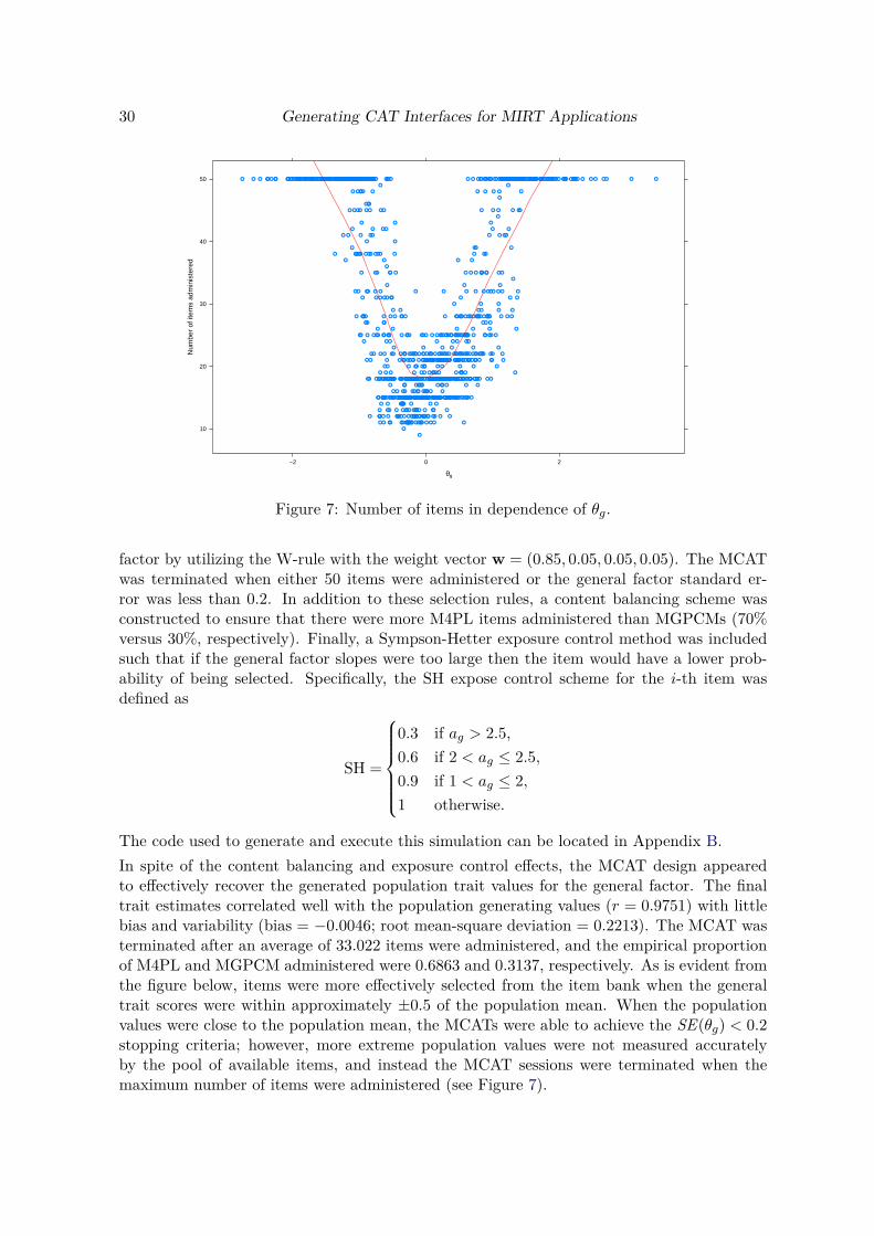
30 Generating CAT Interfaces for MIRT Applications
θg
Num
ber
of it
ems
adm
inis
tere
d
10
20
30
40
50
−2 0 2
● ●
●●
●
●
●
●●
●
●
●
●
●
●
●
●
●
●
●
●
●
●
●
●
●
●
●
●
●●● ●
●
●
●
●
●
●●●
●
●
●
●
●
●
●
●
●
●●
●
●
●
●●
●
●
●
●
●
●
●
●
●
●
●
●
●
●
●
●
●
●
●
●
●
● ●
●
●
● ● ●
●
●●
●
●
●
●
●
●
●
●
●
●
●
●●
●
●
●
●
●
●
●
●
●
●
●
●
●
●
●●
●
●
●
● ●
●
●
●
●
● ●
●
●
●
●
●
●
●
●
●
●
●
●
● ● ●
●●
●
● ●
●
●
●
●
● ●
●
●
●
●
●
●
●
●
●
●
●
●
●
●
●
●
●● ●
●
●
●●
●
● ●
●
● ●
●
●
●
●
●
●
●
●● ●
●
●
●
●
●
●
●
●
●
●
●
●
●
●
●
●
●
● ●
●
●
●
●
●●
●
●
●
●
●
●
●
●
●
●
● ●
●
●
●
●
●
●
●
●
●
●
●
●
●
● ●
●
●
●
●
●
●
●
●
●
●
●
●
●
●
●
●
●
●
●
●
●
●
●●
●
● ●
●●
●
●●
●
●
●
●
●
●
●
●
●
●
●
●
●
●
●
●
●
●
● ●
●
● ●
●
●
●
●
●
●
●
●
●
●
●
●
●●
●
●
●
●
●
●
●
●
● ●
●
●
●
●
●
●
●
●
●
●
●
● ●
●
●
●
●
●●
●
●
●
●
●
●
●
●
●
●
●
●
●
●
●
●
●
●
●
●
● ●●
●
●
●● ●●
●●
●
●
●
●
●
●
●
●
●
●
●
● ●
●
●●
●
●●
●
●
●
●
●
●
●
●
●
●
●
●
●
●
●
●
●
●
●
●
●
●●
●
●
●
●
●
●
●
●
●
●
●
●
●
●●
●
●
●
●
●
●
●
●
●
●
●
●
●
●
●
●
●
●
●
●
● ●
●
●
●
●
●
●
●
●
●
●
●
●
●
●
●
●
●
●
●
●
●
●
●
● ●
●
●
●
●
●
●
●
●
●
●
●
●
●
●
●
●
●
●
●
●
● ●
●
●
●
●
●
●
● ●
●
●
●
●
●
●
●
●
●
●
●
●
●
●
●●
●●
●
●
●●●
●
●
●
●
●
●
●
●●
●
●
●
●
●
● ●
●
●
●
●
●
●
●
●
● ●
●
●
●
●
●
●
●
●
●
●
●
●
●
●
●
●
●●
●
●
●
●
●
●
●
● ●
●
●
●
●
● ●
●
●
●
●
●
● ●
●
●
●
●
●
●●
●
●
●
●
●
●
●
●
●
●
●
●
●
●
●
●
●
●
●
●
●●
●
●
● ● ●
●
●
●
●
●
●
●
●
● ●●
●
●
●
●
●
●
●
●
●
●
●
●
●
●
●
●
●
●
●
●
●
●
●
●
●
●
●
●
●●
●
●
●
●
●
●
●
●
●●
●
●
● ●●
●
●
●
●
●
●
●
● ●●
●
●●
●
●
● ●
●
●●
●
●
●
●
●
●
●
●
●
●
●
●
●
●
●
●
●
●
●
●
●
●
●
●
●
●
●
●
●
●
●
●
●
●
●
●●●
●
●
●
●
●
●
●
●●
●
●●●
● ●
●
●
●
● ● ●
●
●
●
●
●
●●●
●
●
●
●
●
●
●
●
●
● ●
●● ●
●
●
●
●
●
●
●
●
●
●
●
●
●
●
●
●
●
●
●
●
●
● ●
●
●
●
●
●
●
●
●
●
●
●
●
●
●
●
●
●
●●
●
●
●
●
●
●
●
●
●
●
●
●
●
●●
●
●
●
●
●
●●
●
●
●
● ●●
●
●●
●
●
●
●
●
●
●
●
●
●
●
●
●
●
● ●
●
●
●
●
●
● ●
●
●
●
●
●
●●
●
●
●
●
●
●
●
● ●
●
●
●
●
●
●
●
●
●
●
●●
●
●
●
●
●
●
●
●●
●
●
●
●
●
●
●
● ●
●
●
●
●
●
● ●
●
●
●●
●
●
●●
●
●●● ●
●
●
●
●
●
●
●
●
●
●
●●
●
●
●
●
●
●
●
●
●
●
●
●
●
●
●
●
●
●
●
●
●
●
●
●
●
●
●
●
●
●
●
●
●
●
●
●
●
●
Figure 7: Number of items in dependence of θg.
factor by utilizing the W-rule with the weight vector w = (0.85, 0.05, 0.05, 0.05). The MCATwas terminated when either 50 items were administered or the general factor standard er-ror was less than 0.2. In addition to these selection rules, a content balancing scheme wasconstructed to ensure that there were more M4PL items administered than MGPCMs (70%versus 30%, respectively). Finally, a Sympson-Hetter exposure control method was includedsuch that if the general factor slopes were too large then the item would have a lower prob-ability of being selected. Specifically, the SH expose control scheme for the i-th item wasdefined as
SH =
0.3 if ag > 2.5,0.6 if 2 < ag ≤ 2.5,0.9 if 1 < ag ≤ 2,1 otherwise.
The code used to generate and execute this simulation can be located in Appendix B.In spite of the content balancing and exposure control effects, the MCAT design appearedto effectively recover the generated population trait values for the general factor. The finaltrait estimates correlated well with the population generating values (r = 0.9751) with littlebias and variability (bias = −0.0046; root mean-square deviation = 0.2213). The MCAT wasterminated after an average of 33.022 items were administered, and the empirical proportionof M4PL and MGPCM administered were 0.6863 and 0.3137, respectively. As is evident fromthe figure below, items were more effectively selected from the item bank when the generaltrait scores were within approximately ±0.5 of the population mean. When the populationvalues were close to the population mean, the MCATs were able to achieve the SE(θg) < 0.2stopping criteria; however, more extreme population values were not measured accuratelyby the pool of available items, and instead the MCAT sessions were terminated when themaximum number of items were administered (see Figure 7).
Journal of Statistical Software 31
R> n_items <- laply(result, function(x) length(x$items_answered))R> xyplot(n_items ~ Theta[, 1], xlab = expression(theta[g]),+ panel = function(x, y) {+ panel.xyplot(x, y)+ panel.loess(x, y, span = 0.6, col = "red")+ },+ ylab = "Number of items administered")
6. DiscussionIn this article, an R package was introduced for generating interactive graphical interfacesspecifically for MCAT and non-MCAT designs. The package provided tools to generate andanalyze plausible MCAT responses for use in Monte Carlo simulations, provided functions tosummarize MCAT results, and included utilities to plot the estimation history for multiplelatent traits. The estimation efficiency was contrasted with existent R packages, and variousgraphical user interfaces were constructed to demonstrate how real-time MCAT applicationscan be generated with the mirtCAT package. Using the wide selection of IRT models availablein the mirt package, mirtCAT was able to support the construction of flexible unidimensionaland multidimensional adaptive test designs containing a mixture of IRT models.Test developers may choose to execute their MCAT GUIs locally for single computer admin-istrations or deploy their GUIs over the Internet for remote accessibility. Executing the GUIslocally may require password protecting the questions and answer keys, disabling keyboardshortcuts in the Operating System (i.e., Ctrl + Alt + Delete, Alt + F4, Alt + Tab, andso on), and may require saving the relevant R objects and terminating the R session imme-diately after the testing interface is complete. Executing the MCAT GUIs locally will oftenoffer a more controlled laboratory setting, and generally will help maintain the integrity ofthe item pool. Therefore, local execution of MCAT GUIs is the most recommended approach.Remote deployment of MCAT GUIs, on the other hand, will require the configuration of aserver capable of handling the computations, and may introduce other unwanted issues (suchas Internet connection problems, or slower upload and download times).To date, the only open-source GUI-generating system that has been developed for deployingCATs in real-time has been the Concerto project (Kosinski and Rust 2011). Concerto usesthe catR package as the back-end to perform the computations for unidimensional IRT mod-els. However, an unfortunate complication regarding the Concerto project is that it is notimplemented in R, and instead is executed as a standalone web application where R is used asa computational back-end. This requires the user to obtain extra knowledge regarding how tosetup personal servers to collect the response data, requires learning additional web-interfacetools outside of the R language, and, after these skills have been acquired, the interface isstill currently limited to unidimensional IRT models. With the help of the tools available inmirtCAT, projects such as Concerto may be further extended to include unidimensional andmultidimensional tests, potentially with a mixture of IRT models, in a manner similar to howthe catR package has been adopted to perform the back-end computations in R.Future work on mirtCAT will largely be driven by users who are interested in utilizing thepackage tools in their applied research work. However, a number of potential avenues toexplore may include: better support for classification CATs, more dynamic GUI elements,
32 Generating CAT Interfaces for MIRT Applications
and the inclusion of interactive items responses as the shiny framework continues to mature.Currently, interactive items can be included by pointing to raw HTML stems, although thesedo not directly integrate with the responses to each item. Additionally, more holistic controlover content constraints may be included by providing support for so-called shadow testingdesigns (e.g., Veldkamp and Linden 2002).mirtCAT is written and manipulated entirely within R, thereby allowing seamless transition-ing between data collection using GUIs and further item analysis work with packages such asmirt. Users only need to learn basic R code, understand how to define their item parameterswith mirtCAT or estimate their item parameters with the mirt package, and learn how tomanipulate the simple tools defined in mirtCAT to build a completely automated CAT ap-plication for their own research purposes. The package provides intuitive tools to generateinterfaces for local or server-sided use, uses mirt to perform many of the underlying orga-nizational and computational components, includes powerful Monte Carlo simulation designsupport for CATs and MCATs, and helps to facilitate the collection of respondent data usingadaptive and non-adaptive tests or surveys. When used in conjunction with mirt, mirtCATprovides a fluid and organized work-flow for test developers to collect, as well as analyze,their important response data.
AcknowledgmentsSpecial thanks to Matthew Sigal, Nicklaus Csuzdi, and two reviewers for offering helpfulcomments that improved the quality of this manuscript.
References
Bock R, Aitkin M (1981). “Marginal Maximum Likelihood Estimation of Item Parame-ters: Application of an EM Algorithm.” Psychometrika, 46(4), 443–459. doi:10.1007/bf02293801.
Chalmers RP (2012). “mirt: A Multidimensional Item Response Theory Package for the REnvironment.” Journal of Statistical Software, 48(6), 1–29. doi:10.18637/jss.v048.i06.
Chalmers RP (2015). “Extended Mixed-Effects Item Response Models with the MH-RMAlgorithm.” Journal of Educational Measurement, 52(2), 200–222. doi:10.1111/jedm.12072.
Chalmers RP, Counsell A, Flora DB (2016). “It Might Not Make a Big DIF: ImprovedDifferential Test Functioning Statistics that Account for Sampling Variability.” Educationaland Psychological Measurement, 76(1), 114–140. doi:10.1177/0013164415584576.
Chalmers RP, Flora D (2014). “Maximum-Likelihood Estimation of Noncompensatory IRTModels with the MH-RM Algorithm.” Applied Psychological Measurement, 38(5), 339–358.doi:10.1177/0146621614520958.
Chang HH, Ying Z (1996). “A Global Information Approach to Computerized Adap-tive Testing.” Applied Psychological Measurement, 20(3), 213–229. doi:10.1177/014662169602000303.
Journal of Statistical Software 33
Choi SW, King D (2014). MAT: Multidimensional Adaptive Testing. R package version 2.2,URL https://CRAN.R-project.org/package=MAT.
Eggen T (1999). “Item Selection in Adaptive Testing with the Sequential Probabil-ity Ratio Test.” Applied Psychological Measurement, 23(3), 249–261. doi:10.1177/01466219922031365.
Fisher R (1925). “Theory of Statistical Estimation.” Mathematical Proceedings of the Cam-bridge Philosophical Society, 22(5), 700–725. doi:10.1017/s0305004100009580.
Gibbons R, Darrell R, Hedeker D, Weiss D, Segawa E, Bhaumik DK, Kupfer D, Frank E, Gro-chocinski V, Stover A (2007). “Full-Information Item Bifactor Analysis of Graded ResponseData.” Applied Psychological Measurement, 31(1), 4–19. doi:10.1177/0146621606289485.
Gibbons R, Hedeker D (1992). “Full-Information Item Bi-Factor Analysis.” Psychometrika,57(3), 423–436. doi:10.1007/bf02295430.
Kingsbury G, Zara A (1989). “Procedures for Selecting Items for Computerized Adaptive Test-ing.” Applied Measurement in Education, 2, 359–375. doi:10.1207/s15324818ame0204_6.
Kingsbury G, Zara A (1991). “A Comparison of Procedures for Content-Sensitive Item Selec-tion in Computerized Adaptive Tests.” Applied Measurement in Education, 4(3), 241–261.doi:10.1207/s15324818ame0403_4.
Kosinski M, Rust J (2011). The Development of Concerto: An Open Source Online Adap-tive Testing Platform. Paper presented at the International Association for ComputerizedAdaptive Testing, Pacific Grove.
Kullback S, Leibler R (1951). “On Information and Sufficiency.” The Annals of MathematicalStatistics, 22(1), 79–86.
Linden W (1999). “Multidimensional Adaptive Testing with a Minimum Error-Variance Cri-terion.” Journal of Educational and Behavioral Statistics, 24, 398–412. doi:10.3102/10769986024004398.
Linden W, Glas C (eds.) (2010). Elements of Adaptive Testing. Springer-Verlag.
Lord F (1980). Applications of Item Response Theory to Practical Testing Problems. LawrenceErlbaum Associates, Hillsdale.
Magis D, Raîche G (2012). “Random Generation of Response Patterns under ComputerizedAdaptive Testing with the R Package catR.” Journal of Statistical Software, 48(8), 1–31.doi:10.18637/jss.v048.i08.
Maydeu-Olivares A, Hernández A, McDonald RP (2006). “A Multidimensional Ideal PointItem Response Theory Model for Binary Data.” Multivariate Behavioral Research, 41(4),445–471. doi:10.1207/s15327906mbr4104_2.
McBride J, Martin J (1983). “Reliability and Validity of Adaptive Ability Tests in a MilitarySetting.” In DJ Weiss (ed.), New Horizons in Testing, pp. 223–236. Academic Press, NewYork.
34 Generating CAT Interfaces for MIRT Applications
Mulaik S (2010). Foundations of Factor Analysis. 2nd edition. Chapman & Hall, Boca Raton.
Mulder J, Linden W (2009). “Multidimensional Adaptive Testing with Optimal Design Crite-ria for Item Selection.” Psychometrika, 74(2), 273–296. doi:10.1007/s11336-008-9097-5.
Muraki E (1992). “A Generalized Partial Credit Model: Application of an EM Algorithm.”Applied Psychological Measurement, 16, 159–176. doi:10.1177/014662169201600206.
Muraki E, Carlson E (1995). “Full-Information Factor Analysis for PolytomousItem Responses.” Applied Psychological Measurement, 19, 73–90. doi:10.1177/014662169501900109.
Nydick S (2014). catIrt: An R Package for Simulating IRT-Based Computerized AdaptiveTests. R package version 0.5-0, URL https://CRAN.R-project.org/package=catIrt.
Reckase MD (2009). Multidimensional Item Response Theory. Springer-Verlag, New York.doi:10.1007/978-0-387-89976-3.
Revuelta J (1998). “A Comparison of Item Exposure Control Methods in ComputerizedAdaptive Testing.” Journal of Educational Measurement, 35(4), 311–327. doi:10.1111/j.1745-3984.1998.tb00541.x.
RStudio Inc (2014). shiny: Web Application Framework for R. R package version 0.10.0, URLhttps://CRAN.R-project.org/package=shiny.
Samejima F (1969). Estimation of Latent Ability Using a Response Pattern of Graded Scores.Number 17 in Psychometric Monographs. Psychometric Society, Richmond.
Segall D (1996). “Multidimensional Adaptive Testing.” Psychometrika, 61(2), 331–354. doi:10.1007/bf02294343.
Suh Y, Bolt D (2010). “Nested Logit Models for Multiple-Choice Item Response Data.”Psychometrika, 75(3), 454–473. doi:10.1007/s11336-010-9163-7.
Sympson J (1977). “A Model for Testing with Multidimensional Items.” In D Weiss (ed.), Pro-ceedings of the 1977 Computerized Adaptive Testing Conference, pp. 82–98. ComputerizedAdaptive Testing Laboratory, Minneapolis.
Thissen D (1982). “Marginal Maximum Likelihood Estimation for the One-Parameter LogisticModel.” Psychometrika, 47(2), 175–186. doi:10.1007/bf02296273.
Thissen D, Cai L, Bock R (2010). “The Nominal Categories Item Response Model.” In M Ner-ing, R Ostini (eds.), Handbook of Polytomous Item Response Theory Models: Developmentand Applications, pp. 43–75. New York: Taylor & Francis.
Thissen D, Pommerich M, Billeaud K, Williams V (1995). “Item Response Theory for Scoreson Tests Including Polytomous Items with Ordered Responses.” Applied Psychological Mea-surement, 19(1), 39–49. doi:10.1177/014662169501900105.
Veldkamp B, Linden W (2002). “Multidimensional Adaptive Testing with Contsraints onTest Content.” Psychometrika, 67(4), 575–588. doi:10.1007/bf02295132.
Journal of Statistical Software 35
Veldkamp B, Linden W (2008). “Implementing Sympson-Hetter Item-Exposure Control in aShadow-Test Approach to Constrained Adaptive Testing.” International Journal of Testing,8(3), 272–289. doi:10.1080/15305050802262233.
Wainer H, Dorans N (eds.) (2000). Computerized Adaptive Testing: A Primer. 2nd edition.Lawerence Erlbaum Associates.
Warm T (1989). “Weighted Likelihood Estimation of Ability in Item Response Theory.”Psychometrika, 54(2), 427–450. doi:10.1007/bf02294627.
Weiss D (1982). “Improving Measurement Quality and Efficiency with Adaptive Testing.”Applied Psychological Measurement, 6(4), 479–492. doi:10.1177/014662168200600408.
Wickham H (2011). “The Split-Apply-Combine Strategy for Data Analysis.” Journal ofStatistical Software, 40(1), 1–29. doi:10.18637/jss.v040.i01.
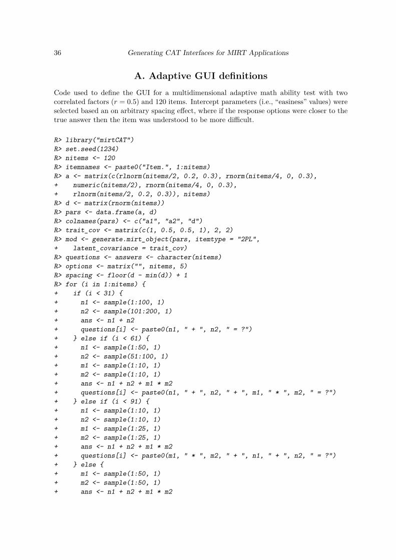
36 Generating CAT Interfaces for MIRT Applications
A. Adaptive GUI definitionsCode used to define the GUI for a multidimensional adaptive math ability test with twocorrelated factors (r = 0.5) and 120 items. Intercept parameters (i.e., “easiness” values) wereselected based an on arbitrary spacing effect, where if the response options were closer to thetrue answer then the item was understood to be more difficult.
R> library("mirtCAT")R> set.seed(1234)R> nitems <- 120R> itemnames <- paste0("Item.", 1:nitems)R> a <- matrix(c(rlnorm(nitems/2, 0.2, 0.3), rnorm(nitems/4, 0, 0.3),+ numeric(nitems/2), rnorm(nitems/4, 0, 0.3),+ rlnorm(nitems/2, 0.2, 0.3)), nitems)R> d <- matrix(rnorm(nitems))R> pars <- data.frame(a, d)R> colnames(pars) <- c("a1", "a2", "d")R> trait_cov <- matrix(c(1, 0.5, 0.5, 1), 2, 2)R> mod <- generate.mirt_object(pars, itemtype = "2PL",+ latent_covariance = trait_cov)R> questions <- answers <- character(nitems)R> options <- matrix("", nitems, 5)R> spacing <- floor(d - min(d)) + 1R> for (i in 1:nitems) {+ if (i < 31) {+ n1 <- sample(1:100, 1)+ n2 <- sample(101:200, 1)+ ans <- n1 + n2+ questions[i] <- paste0(n1, " + ", n2, " = ?")+ } else if (i < 61) {+ n1 <- sample(1:50, 1)+ n2 <- sample(51:100, 1)+ m1 <- sample(1:10, 1)+ m2 <- sample(1:10, 1)+ ans <- n1 + n2 + m1 * m2+ questions[i] <- paste0(n1, " + ", n2, " + ", m1, " * ", m2, " = ?")+ } else if (i < 91) {+ n1 <- sample(1:10, 1)+ n2 <- sample(1:10, 1)+ m1 <- sample(1:25, 1)+ m2 <- sample(1:25, 1)+ ans <- n1 + n2 + m1 * m2+ questions[i] <- paste0(m1, " * ", m2, " + ", n1, " + ", n2, " = ?")+ } else {+ m1 <- sample(1:50, 1)+ m2 <- sample(1:50, 1)+ ans <- n1 + n2 + m1 * m2

Journal of Statistical Software 37
+ questions[i] <- paste0(m1, " * ", m2, " = ?")+ }+ answers[i] <- as.character(ans)+ ch <- ans + sample(c(-5:-1, 1:5) * spacing[i, ], 5)+ ch[sample(1:5, 1)] <- ans+ options[i,] <- as.character(ch)+ }R> df <- data.frame(Question = questions, Option = options, Answer = answers,+ Type = "radio")
B. Code to generate MCAT simulationCode used to generate and analyze a multidimensional mixed-item simulation with mirtCAT.
R> library("mirtCAT")R> library("plyr")R> library("mvtnorm")R> nitems <- 360R> N <- 1000R> a <- matrix(c(rlnorm(nitems, 0.2, 0.3),+ rlnorm(nitems/3, -1, 0.2), numeric(nitems),+ rlnorm(nitems/3, -1, 0.2), numeric(nitems),+ rlnorm(nitems/3, -1, 0.2)), nitems, 4)R> d <- data.frame(d = rnorm(nitems/2))R> g <- c(rep(0.2, nitems/2), rep(NA, nitems/2))R> u <- c(rep(0.95, nitems/2), rep(NA, nitems/2))R> ds <- data.frame(matrix(rnorm(nitems*2, 0, 2), nitems/2, 4))R> ints <- rbind.fill(d, ds)R> pars <- data.frame(a, g, u, ints)R> colnames(pars) <- c(paste0("a", 1:4), "g", "u", "d", paste0("d", 1:4))R> itemtype <- c(rep("4PL", nitems/2), rep("gpcm", nitems/2))R> mo <- generate.mirt_object(pars, itemtype)R> Theta <- rmvnorm(N, sigma = diag(4))R> resp <- generate_pattern(mo, Theta)R> SH <- rep(1, nitems)R> SH <- ifelse(a[, 1] > 1, 0.9, SH)R> SH <- ifelse(a[, 1] > 2, 0.6, SH)R> SH <- ifelse(a[, 1] > 2.5, 0.3, SH)R> content <- rep(c("4PL", "gpcm"), each = nitems/2)R> content_prop <- c("4PL" = 0.75, "gpcm" = 0.25)R> design <- list(min_SEM = c(.2, Inf, Inf, Inf),+ weights = c(0.85, 0.05, 0.05, 0.05), max_items = 50,+ exposure = SH, content = content, content_prop = content_prop)R> library("parallel")R> cl <- makeCluster(detectCores())R> result <- mirtCAT(mo = mo, local_pattern = resp, start_item = "Wrule",

38 Generating CAT Interfaces for MIRT Applications
+ criteria = "Wrule", design = design, cl = cl)R> est.Theta1 <- laply(result, function(x) x$thetas[1])R> ave_nans <- mean(laply(result, function(x) length(x$items_answered)))R> empirical_contents <- ldply(result, function(x, content)+ table(content[x$items_answered]) / length(x$items_answered),+ content = content)R> empirical_props <- colMeans(empirical_contents)R> r <- cor(Theta[,1], est.Theta1)R> bias <- mean(Theta[,1] - est.Theta1)R> RMSD <- sqrt(mean((Theta[,1] - est.Theta1)^2))
Affiliation:R. Philip ChalmersDepartment of PsychologyYork University4700 Keele St.Toronto, ON, M3J 1P3, CanadaE-mail: [email protected]
Journal of Statistical Software http://www.jstatsoft.org/published by the Foundation for Open Access Statistics http://www.foastat.org/
July 2016, Volume 71, Issue 5 Submitted: 2014-08-15doi:10.18637/jss.v071.i05 Accepted: 2015-05-25