Generation of numerical human models based on …publications.lib.chalmers.se/records/fulltext/local_155348.pdf · Generation of numerical human models based on medical imaging

Generation of numerical human models

based on medical imaging

Research Report in Mechanical Engineering

MARTA GONZALEZ CARCEDO

KARIN BROLIN

Department of Applied Mechanics

Division of Vehicle Safety

CHALMERS UNIVERSITY OF TECHNOLOGY

Göteborg, Sweden 2012

Research Report 2012:01

RESEARCH REPORT 2012:01

Generation of numerical human models based

on medical imaging

MARTA GONZÁLEZ CARCE D O

KARIN BROLIN




Göteborg, Sweden, 2012

Generation of numerical human models based on medical

imaging.

M A R T A G O N Z Á L E Z C A R C E D O

K A R I N B R O L I N

© M A R T A G O N Z A L E Z C A R C E D O , K A R I N B R O L I N , 2012

Research report 2012:01

ISSN 1652-8549




SE-412 96 Göteborg

Sverige

Telephone +46 (0)31 772 1000

Cover:

Generation of numerical human models based on medical imaging.

Chalmers Reproservice

Göteborg, Sweden 2012

CHALMERS, Applied Mechanics, Research Report 2012:01

I

Generation of numerical human models based on medical imaging

Research Report in Mechanical Engineering

MARTA GONZALEZ CARCEDO

KARIN BROLIN Department of Applied Mechanics


Chalmers University of Technology

ABSTRACT

The aim of this project was to increase the knowledge of how

numerical models can be generated based on medical imaging data.

The software used was Scan IP+FE/+CAD (Simpleware Ltd, UK).

Three studies were conducted to generate models for Computer Fluid

Dynamics (CFD) and Finite Element (FE) analysis, focusing on the

medical imaging process. The real geometry of an aorta with a stent

graft was generated based on Computer Tomography (CT) images

from two patients. Several meshes were generated, evaluated and

exported to OpenFOAM for CFD analysis. It was possible to run the

simulation. Two FE models of the cervical vertebrae were generated

based on CT images of female necks. The mesh density needed to

capture joint slope and other important features were investigated.

Lastly, image processing of rat and monkey head, brain and neck was

performed to extract anatomical details and compare brain size with

specimen mass.

This project was finalized with a workshop to spread the gained

knowledge to the graduate students and researchers at the Department

of Applied Mechanics of Chalmers, active in the field of human body

modeling, and open to participants from partners of the SAFER -

Vehicle and Traffic Safety Center- at Chalmers and the Strategic Area

of Transport at Chalmers.

Key words: Medical imaging, numerical models, meshing, aorta, cervical spine,

animals models


II

CHALMERS, Applied Mechanics, Research Report 2012:01 III

Contents

ABSTRACT I

CONTENTS III

PREFACE V

TERMINOLOGY VI

1 SCOPE OF THE PROJECT 1

2 METHOD 2

2.1 Import and pre-processing data 2

2.2 Segmentation 2

2.3 Three Dimensional Analysis 3

2.4 Surface extraction, meshing and exporting 3

3 AORTA PROJECT 4

3.1 Background 4

3.2 Work process 4

3.2.1 Data 4

3.2.2 Segmentation process – Stent graft 5

3.2.3 Segmentation process –Noise 6

3.2.4 Segmentation process - The aneurysm dilatation artery 7

3.2.5 3D Analysis – Comparison of models 8

3.2.6 Computational Fluid Dynamic mesh generation 10

3.2.7 Extract geometry and do CFD meshing with other software 13

3.3 Conclusion 14

3.4 Future work 15

4 FEMALE NECK PROJECT 17

4.1 Background 17

4.2 Work process 17

4.2.1 Data used 17

4.2.2 Segmentation process. 18

4.2.3 3D Analysis – Comparison of models 20

4.2.4 Comparing the angles of contacts surfaces 20

4.2.5 Finite Element mesh generation 23

4.3 Conclusion 26

4.4 Future work 27

5 ANIMALS MODELS PROJECT 28

CHALMERS, Applied Mechanics, Research Report 2012:01 IV

5.1 Rat project 28

5.1.1 Background 28

5.1.2 Work process 28

5.2 Monkey project 37

5.2.1 Background 37

5.2.2 Work process 38

5.3 Conclusion and future work 40

6 WORKSHOP 41

6.1 Contents 41

6.1.1 Initial presentation 41

6.1.2 Hand-on exercise during the week 42

6.1.3 Final presentation 42

6.2 Hand-on Applications 42

6.2.1 Active Human Body Models project: Applications for medical image

processing 45

6.2.2 Injury-HBM project 46

6.3 Feedback 46

6.4 What did you learn? 46

6.5 Value of the workshop? 47

6.6 Feedback on the program/planning. 47

6.7 Conclusions 47

6.8 Lesson learned 48

7 REFERENCES 49

8 APPENDICES 50

CHALMERS, Applied Mechanics, Research Report 2012:01 V

Preface

This work was possible through funding from Chalmers‟ Transport Area of Advance;

project ‟Humanmodellering för skadeprevention„. This work was carried out at the

SAFER -Vehicle and Traffic Safety Centre at Chalmers during three months in the

fall of 2011. The project was initiated by the Human Body Modelling group at the

Department of Applied Mechanics: Karin Brolin, Håkan Nilsson, Håkan Johansson,

and Kenneth Runesson.

This project, all the imaging work with the software and the documentation were

carried out by Marta Gonzalez Carcedo under the supervision of Karin Brolin.

Simpleware Ltd is acknowledged for their kind cooperation and support throughout

this project and for supplying extra licenses for the workshop. It would not have been

possible without you!

The project would not have been successful without the active participation of Håkan

Nilsson from Chalmers, Håkan Roos from Sahlgrenska University Hospital, Jacobo

Antona Makoshi from JARI (Japan Automobile Research Institute) and Chalmers, and

Ermes Tarallo from Politecnico di Milano.

Göteborg December 2011

Marta González Carcedo and Karin Brolin.

CHALMERS, Applied Mechanics, Research Report 2012:01 VI

Terminology

Variables that are occurring in this report:

AHBM Active Human Body Model.

Atlas First cervical vertebrae, C1.

Axis Second cervical vertebrae C2.

Background data To refer the image volume grey scale data.

C1, C2… C7 Cervical vertebrae number 1, 2,…,7.

CAD Computer Aided Design.

Cervical spine Superior region of the spine with 7 vertebrae.

CFD Computational Fluid Dynamics.

Cortical bone Compact bone at the surface of the vertebrae.

CT Computed Tomography.

DICOM Digital Imaging and Communication in Medicine.

EVAR Endovascular Aortic Repair.

FE Finite Element

HU Hounsfiel Units.

Intervertebral disc Soft tissue joint in the spine, connecting two adjacent

vertebrae.

MRI Magnetic Resonance Imaging.

Occipitoatlantal joint Joint between the occiput and the first cervical vertebra, C1.

T1 First thoracic vertebrae.

Trabecular bone Porous bone in the centre of the vertebrae.

3D model Three Dimensional model


1

1 Scope of the project

The aim of this project was to increase the knowledge of how numerical models can

be generated based on medical imaging data. The used software was Scan

IP+FE/+CADv4.3 (Simpleware Ltd, Exeter, UK). It included creating models for

three applications:

Aorta for Computational Fluid Dynamic (CFD) simulation of stent graft (see

section 3),

Female neck for Finite Element (FE) analysis (see section 4), and

Different aspect of image processing of animals models (see section 5).

The project was finalised with a workshop to spread the gained knowledge to the PhD

students and researchers at the Department of Applied Mechanics, active in the field

of human body modelling or with an interest in image processing (see section 6).

Figure 1: Aorta with aneurysm and stent graft (left), female neck model (middle), and monkey and rat head and brain models (right).


2

2 Method

The aim of this project is to explore how numerical models can be generated based on

medical imaging data. Computer Tomography (CT) is a medical imaging method that

can be employed to generate three dimensional geometries, based on a stack of

images.

The software ScanIP+FE/+CADv4.3 (Simpleware Ltd, Exeter, UK) was used for the

image processing and model generation. The method is based in four basic functions

(Figure 2):

- Importing and pre-processing data ( see section 2.1),

- Segmentation (see section 2.2),

- 3D Analysis (see section 2.3) and

- Surface extraction, meshing and exporting data (see section 2.4).

Figure 2: Scan to model

2.1 Import and pre-processing data

The first step is to import data and prepare it. The images can be manipulated, through

the process of windowing. It is possible to remove the noise through a filtering

process. In addition, it adjusts the data so the size of the object is correct and/or

reduces the amount of data to work with.

2.2 Segmentation

Segmentation is the process of partitioning a digital image into multiple segments.

Focus in the current project is on the process where the different organs and bones are

identified in the slides. In a region of interest, the pixels are similar with respect to

some characteristic, such as colour, intensity or texture. Based on this, the different

regions are identified inside the image and the masks can be created.

Some knowledge of the X-ray attenuation of normal structures is useful to assist

interpretation of the images. The Hounsfield scale measures radio density. In air its

value is -1000 HU (Hounsfield Units), in pure water it is 0 HU.

The software offers semiautomatic segmentation tools based on different techniques,

such as threshold or region-growing. In addition, it offers a wide range of filters for

different applications. Incorrect use of the filter can cause loss of characteristics of the

shape and size of model. The filters and the number of iterations depend on the data

and the model that it is generated.


3

2.3 Three Dimensional Analysis

In this step the 3D model can be analysed and different geometrical measures can be

performed.

2.4 Surface extraction, meshing and exporting

It is possible create a CAD surface, and CFD and FE models. The model is exported

directly to several formats compliant to commercial software. It is possible export

additional information together with the model, such as interface relationship,

material properties, etc.

Some tools require some expertise and practice in order to give satisfactory results.

There could be many ways of getting the same results. The key is to find the quickest

way and the experience will improve your efficiency!


4

3 Aorta Project

This project was realized in cooperation with Håkan Nilsson from Chalmers and

Håkan Roos from Sahlgrenska University Hospital. The main interest of this project is

to extract the real geometry of a stent-graft to perform CFD analyses with the

software OpenFOAM.

3.1 Background

Abdominal aortic aneurysm is a dilatation of the abdominal aortic vessel. It occurs

most often in individuals over 65 years of age and is more common among men and

smokers. The classical treatment of the abdominal aortic aneurysm consists in an open

operation to replace the affected vessel wall with prosthesis; this is a large operation

with significant morbidity and mortality. Since mid 1990‟s a minimally invasive

technique is also available, a stent grafts is inserted in the aorta to prevent rupture. .

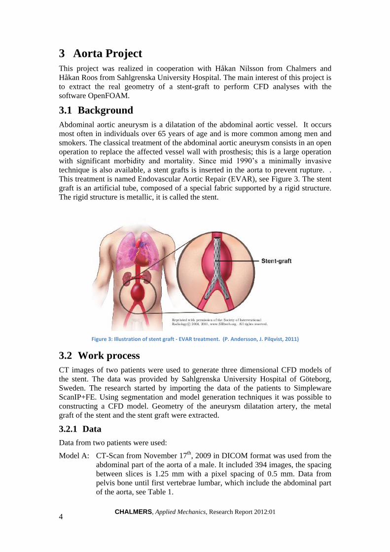
This treatment is named Endovascular Aortic Repair (EVAR), see Figure 3. The stent

graft is an artificial tube, composed of a special fabric supported by a rigid structure.

The rigid structure is metallic, it is called the stent.

Figure 3: Illustration of stent graft - EVAR treatment. (P. Andersson, J. Pilqvist, 2011)

3.2 Work process

CT images of two patients were used to generate three dimensional CFD models of

the stent. The data was provided by Sahlgrenska University Hospital of Göteborg,

Sweden. The research started by importing the data of the patients to Simpleware

ScanIP+FE. Using segmentation and model generation techniques it was possible to

constructing a CFD model. Geometry of the aneurysm dilatation artery, the metal

graft of the stent and the stent graft were extracted.

3.2.1 Data

Data from two patients were used:

Model A: CT-Scan from November 17th

, 2009 in DICOM format was used from the

abdominal part of the aorta of a male. It included 394 images, the spacing

between slices is 1.25 mm with a pixel spacing of 0.5 mm. Data from

pelvis bone until first vertebrae lumbar, which include the abdominal part

of the aorta, see Table 1.


5

Model B: CT-scan from September 5th

, 2011 in DICOM format was used from

abdominal part of the aorta of a male. It included 349 images, the spacing

between slices is 1.60 mm with a pixel spacing of 0.7 mm. Data from third

thoracic vertebrae until the pelvis bone, including thoracic and abdominal

aorta, see Table 1.

Table 1: Specification of image data.

Data from Data

type Gender

Age

(Y)

Series

no Images

Pixel

spacing

(mm)

Spacing

between slices

(mm)

Model A CT Male 74 6 394 0.5 1.25

Model B CT Male 77 8377 349 0.7 1.6

3.2.2 Segmentation process – Stent graft

The stent graft is an artificial tube, composed of a special fabric supported by a rigid

structure. The rigid structure is metallic and has a high density in comparison to the

rest of the soft tissues, which makes the identification process easier.

Figure 4 shows a CT scan taken around the thoracic level, where the aorta is situated

between the lungs. The spine and the ribs can be easily identified, in the same way

that the metallic parts of the stent graft. In the center of the image the circular

geometry with bright color is the metallic parts of the stent graft. The stent has a very

thin layer of fiber that is just inside the metal, but it is not possible to see in these

images. A radiopaque contrast liquid is injected into the blood for easier visualization

of the vessel lumen.

The 2D image data gives a lot of information, and the three dimensional models is

predicted with the 2D cross sections. In Figure 4 the stent graft shows a circular cross

section, in contrast to Figure 5 that shows a more oval shape. It is caused by the

direction of the scanner that is not perpendicular to the cross section of the stent in

that area.

Figure 4: CT image from the Stent graft thoracic-abdominal part.

Figure 5: CT image from the Stent graft thoracic-abdominal part

Two regions were defined in the stent graft: the fluid and the solid region see Figure

6. The fluid is assumed to be inside the stent. The solid region is assumed as a thin

layer on the inside of the stent. In this project the main interest is generation of a mesh

for the fluid region and assumes that the solid region is stiff. So, the boundary

conditions for the fluid region can be set at the border of that region.


6

Confidence connected region growing segmentation techniques was used to extract

the geometry of the fluid region. Then, filters to fill cavity and avoid holes were

applied. 3D editing tools were using to delete another vessels and smooth specific

regions. Using Boolean operation, an additional layer that surround the fluid region is

created for the solid region. Flat surface in the boundary were generate by cutting the

image in the boundary patches and sharp edges were obtained, see Figure 7.

Figure 6: Solid and fluid region of the stent graft

Figure 7: boundary patches it is necessary patches with sharp edges perpendicular to the vanes

Metal graft of the stent with high density can easily be identified in the images. Using

threshold segmentation techniques the geometry is extracted. Manual tools are

necessary to reconstruction the parts where metal artifacts disturb the image data. This

can be seen in the upper part of the one of the legs, see Figure 8 and a change of the

diameter is identified Figure 9. It is due to a smaller diameter of the stentgraft at the

overlap between two stentgrafts. The thinner leg has a standard diameter and the

extension is chosen depending on the width of the artery, see Figure 10. The CAD

surface of the metal graft of the stent was extracted to analysis its geometry.

3.2.3 Segmentation process –Noise

The data shows some noise in different part caused by the metallic part of the stent

graft. The presence of metal objects in the scan leads to reflections in the image and

hides the geometry of these parts. This is called “metal artifacts”, it shown in Figure

11. The parts affected by this phenomenon need to be reconstructed. Noise filters are

available to reduce the metal artifact or manual tools can be used. In this project,

manual tools were used to reconstruct the geometry. The geometry in these areas was

created, basing on the interpolation between neighboring cross sections without the

metal artifact.

Figure 8: CT image where it is possible to see the high density

area of the stent graft.

Figure 9: Diference of diameter in one of the legs.

Figure 10: Metal graft of the stent.


7

Figure 11: Metal arifacts in CT image.

3.2.4 Segmentation process - The aneurysm dilatation artery

Using flood fill and morphological filter, the geometry of the aneurysm dilatation

artery was extracted. In the aneurysm dilatation the geometry is well defined, Figure

12. But in the other parts, the layer of the artery is close to the stent, Figure 13. The

metal parts hide the geometry of the artery in this region and make it hard to follow

the geometry. In these areas the outer boundary of the geometry needs to be assumed.

Figure 12: Aneurysm dilatation artery in CT image

Figure 13: artery and stent graft in CT image

Figure 14: 3D Model of the aneurysm dilatation based on

CT data ModelB.

The Figure 15 shows the histogram of the background of data from Model A. It shows

the number of pixels with different intensity. The histogram allows seeing the

frequency of the grey scale value belonging to the images. This is useful to analysis

the peaks and valleys in the histogram and it is used to locate the clusters in the

image. Based in the histogram and using threshold methods, the different regions can

be defined. The stent fluid region can be defined from 250 to 400 in the grey scale.

The metallic parts show high values from 400 to 800 in the grey scale and the

aneurysm dilatation is in the range from 0 to 200 in the grey scale.


8

Figure 15: Histogram background CT data from Model A.

3.2.5 3D Analysis – Comparison of models

The geometry of the aneurysm dilatation and the stent graft was extracted for both

models. Figure 16 shows a view of the aneurysm dilatation model and the stent graft

based on CT data images from Model A. Figure 17 shows a view of the aneurysm

dilatation model and the stent graft based on CT data images from Model B. A visual

three dimensional comparison can be performed. The models has, in the fluid region,

different geometry where Model B is very twisted, see Figure 17.

In Model A, one of the legs has a change of the diameter. It is because the long leg is

generally made with a width that corresponds to the vessel and can therefore have

different dimensions. The short leg is in this case 12 mm in diameter and the long

contralateral leg is 16 mm in diameter see Figure 18. A high density of metallic is

showed in this area that the diameter changes. It is due the contralateral leg is inserted

in the leg. The geometry of the metal graft of the stent in this area is difficult to

extract. In Model B, the difference between diameters is showed in the region after

the aneurysm dilatation, see Figure 19. Where the aneurysm is dividing in two legs,

there is a reduction in the diameter and later the diameter is increased.

The aneurysm dilatation 3D models are shown in Figure 20 for Model A and in Figure

21 for Model B. Model A has a larger diameter compared to the other. The model A

(Figure 20) shows a diameter ten times smaller than the other. The aneurysm

dilatation based in Model A is 63 mm. while in Model B it is 73 mm.


9

Figure 16: 3D Model of the aneurysm dilatation and the stent graft based on CT data Model A

Figure 17: 3D Model of the aneurysm dilatation and the stent graft based on CT data Model B

Figure 18: 3D Model of the stent based on CT data Model A . There is a change in the diameter in one of

the legs.

Figure 19: 3D Model of the stent based on CT data Model B. The change of the diameter after the

dilatation is shown.

Figure 20: 3D Model of the aneurysm dilatation and based on CT data Model A.

Figure 21: : 3D Model of the aneurysm dilatation based on CT data Model B.


10

3.2.6 Computational Fluid Dynamic mesh generation

The main interest of this project is the mesh of the fluid region. The CFD mesh was

generated with ScanIP+FE and exported to OpenFOAM through the Fluent format,

then an OpenFOAM utility is used to convert the mesh to OpenFOAM format

(fluentMeshToFoam).

The CFD mesh of the fluid and the solid region and the aneurysm dilatation without

the stent were generated for both models. The CAD surface from the aneurysm

dilatation artery was exported as STL format for both models and the metal graft of

the stent for Model A. The geometry of the stent was extracted and the CFD mesh

generate with ScanIP+FE. Two different meshes were generated: fluid and solid mesh

based in the two regions in Figure 22.

In the mesh of the fluid region the interior is less important so it can have a coarse

mesh, Figure 23. Instead, close to the boundary it is very important to have boundary

layers of cells with a high number of elements. Based on this, the mesh of this region

is defined with coarse mesh in the interior and refined close to the boundaries, having

a smaller length edge close to the boundary, as in the mesh Figure 24. Of course, this

will increase the total number of cells. Another possibility is to generate a boundary

layer with small cells, as in the model Figure 25. This option increases considerably

the number of cells.

In the solid region, there can be a high number of cells. Figure 26 shows the mesh of

the solid region. If the mesh is refined in this region it is possible create cells with

small length edge, see the Figure 27. These tetrahedral meshes were created with

ScanIP+FE. It is possible to import to OpenFOAM and run a simulation.

A CFD mesh of the fluid region from data ModelA was generated. The mesh was

created with tetrahedrons and defined with coarse mesh in the interior and refined

close to the boundary, but with low number of elements, similar too Figure 23. It was

exported with 31,555 cells and the target minimum edge length of 2 mm. and a

maximum length of 5 mm. The material was defined as a fluid. Four boundaries

condition are included: fluid region to background, fluid region, fluid region to Zmin,

and fluid region to Zmax, see Figure 28. The mesh was imported directly from

ScanIP+FE and it was run in OpenFOAM. The mesh is exported in millimeters.

Steady flow was realized, the Figure 29 shows the image of a steady flow of the fluid

region of the stent graft in the aortic aneurysm.

In addition, another CFD mesh from the same model, the fluid region of Model A was

extracted. It was generated mixing hexahedral and tetrahedral but it was not possible

to import into OpenFOAM.


11

Figure 22: The fluid and the solid mesh of the stent are shown.

Fluid

Mesh

Figure 23: Fluid region with coarse interior mesh.

Figure 24: Fluid region with coarse interior mesh and refine in close to

the boundary.

Figure 25: Fluid region with coarse interior mesh and refine a

boundary layer of cells.

Solid

Mesh

Figure 26: Solid region mesh.

Figure 27: Solid region mesh is refined.

Figure 28: boundary conditions are defined.

Figure 29: Steady flow in stent graft in an aortic aneurysm


12

After the research to know that it was possible to import directly and run a simulation.

The tetrahedral CFD mesh from the stent fluid region and aneurysm aortic dilatation

was extracted from both models. In addition the CAD surface in STL format from the

metallic stent was exported.

In the pre-processing process smoothing was applied and the boundary conditions

were defined. The models were exported to the CFD format for the software Fluent.

CFD mesh and STL of the aneurysm aortic dilatation from Model B was

exported with 17693 nodes and 71241 tetrahedral cells; Boundary conditions

defined: From aneurysm to background, aneurysm, from aneurysm to Zmin,

from aneurysm to Zmax; Figure 30.

CFD mesh and STL of the Stent Fluid region from Model B was exported with

36416 nodes and 142483 tetrahedral cells. Boundary conditions defined: From

Fluid to background, Fluid, from Fluid to Zmin, from Fluid to Zmax; Figure

31.

CFD mesh and STL of the aneurysm aortic dilatation from Model A was

exported with 19372 nodes and 81517 tetrahedral cells; Boundary conditions

defined: From aneurysm to background, aneurysm, from aneurysm to Zmin,

from aneurysm to Zmax; Figure 33.

CFD mesh and STL of the Stent Fluid region from Model A: model export to

fluent volume with 12609 nodes, 48547 tetrahedral cells. Faces: From Fluid to

background, Fluid, from Fluid to Zmin, from Fluid to Zmax; Figure 34.

CAD surface in STL format of the Metallic stent from Model A were exported

with target minimum edge length 1 mm. and maximum 3 mm. Figure 35.

In the pre-processing smoothing was applied and the boundary conditions were

defined. The cross section of the inlets and outlets where define in the same place for

the stent and in the aneurysm aortic dilatation, see Figure 32 and Figure 35. The

models were exported to CFD fluent format.


13

Figure 30: CFD Model of the aneurysm dilatation based on CT data Model B

Figure 31: CFD Model of the stent graft based on CT data Model B

Figure 32: CFD Model of the aneurysm dilatation and the stent graft based on CT data Model B

Figure 33: CFD Model of the aneurysm dilatation based on CT data Model A

Figure 34: CFD Model of the stent graft on CT data Model A

Figure 35: CFD Model of the aneurysm dilatation and the stent graft based on CT data Model A

3.2.7 Extract geometry and do CFD meshing with other software

In this project, the possibility of combining different software was explored. So the

geometry is extracted base from the image processing method using ScanIP+FE.

Then, the CAD surface from the model was exported in STL file format, which was

used to generate a mesh with software ICEM CFD.

The mesh generation process was realized by Håkan Nilsson and the model meshing

is showed Figure 36. The mesh can be generated with hexahedral cells. For this

geometry the mesh generated with ICEM CFD shows easier control and more

flexibility of the mesh.


14

Figure 36: Geometry was extracted with Simpleware by Marta Gonzalez Carcedo and mesh was generated with ICEM CFD by Håkan Nilsson.

3.3 Conclusion

Two models were extracted from data of two different patients. The geometry of the

aneurysmal dilatation of the artery, the metal graft of the stent and the stent graft were

extracted. A three dimensional analysis was performed.

The quality of CT data from Model B is not enough to extract the geometry of the

metallic parts. The spacing of the image needs to be smaller to follow the geometry,

and reconstructing the geometry lot of manual work is required. Instead, in Model A,

the geometry was extracted with a high detail.

From the image in 2D can be extracted a lot of information about the model. The stent

has a very thin layer that is just inside the metal, but it is not possible to see in the

image. It is assumed the solid region base in the fluid region extracting a thin layer.

So it is possible to obtain a separate thin wall around the fluid section to generate a

solid mesh. But there is a limitation of definition of the thickness of this layer.

The metallic parts of the stent graft can be easily identified, but to extract the

geometry require some manual work. In addition, the geometry in the areas with high

density of metal graft or overlapping of the metal wires makes it difficult to follow the

geometry.

It is possible to generate CFD boundary conditions in the mesh. For generation of the

boundary patches it is necessary to have patches with sharp edges perpendicular to the

aorta. One of the ways to keep a flat surface is cropping the image to the point on the

masks where you would like the flat surface to be. However sometimes this is not

possible because the geometry and may require cuts in arbitrary directions. In this

case, another mask is necessary to create in where you would like the flat surface to

be. In this case you can get a flat surface but the edges of the patches are not sharp.

The areas with metal artifacts hide information, so if it is possible it should be avoided

during scanning. The image needs to be reconstructed in these areas. ScanIP+FE has

available a noise filtering of metal artifact reduction that attempts to reduce streaking

artifacts caused by metallic objects in a CT scan. The purpose of the filter is to


15

enhance the high frequencies which correspond to the image edges. This filter is very

useful but consumes a lot of time.

It is flexible to extract measures and analyze the model in 3D.

The process of the CFD mesh generation, it is very useful to extract the real geometry

based on data from the scan. It can be meshed with ScanIP+FE directly with some

flexibility to create the mesh but also it has some limitations:

It is not possible generate a hexahedral mesh. The mesh was generated with

tetrahedral.

There is another algorithm where it is possible to generate the mesh mixing

tetrahedral and hexahedral but this mesh was not possible import into

OpenFOAM. The hexahedral is often generated in the center and the edges are

tetrahedral, but in this case it would be more interesting to the have hexahedral

mesh at the edges. So this solution does not help in this case.

It is possible have a coarse mesh in the interior, where it is not necessary has a

high number of cells, to reduce the number of cells. It is possible to have a

finer mesh close to the boundary, where it is interesting to have a high number

of cells. Also, it is possible to define a small length edge close to the boundary.

It is necessary to achieve better treatment of the boundary layers. However,

this is an area that the Simpleware group has looked at improving and in their

next release (ScanIP v5.0) there will be a new boundary layer option for the

mesh, which will create prism elements at the surfaces rather than tetrahedral,

an example is shown in Figure 37.

It is possible to generate the mesh in ScanIP+FE and import to OpenFOAM.

The main conclusion is that the CFD analysis is a very important field to explore in

the research with medical application. The aim is to find the optimal treatment for

each patient. Here, the images processing is a useful tool to CFD analysis.

Figure 37: An example of boundary layer that will be available in the next release. Image from Simpleware support

3.4 Future work

Two models were extracted from data of two different patients. The main interest of

this project was extracted the real geometry of the stent and analysis of the fluid

region. The model can be improved with better treatment of the boundary layer. It can

be possible to extract a CAD surface and generate the mesh with other software. Also,


16

the model can be improved with better treatment of the boundary layer with the new

release that Simpleware offers.

CFD mesh of the aneurysm dilatation artery was extracted. In this area there is same

inlet that flow in the interior of the aneurysm. It will be interesting to analyse the

blood flow into the aneurysm dilatation and how it influences the blood pressure in

the weak walls caused by the aneurysm dilatation, see Figure 38.

The metal graft of the stent was extracted. Further analysis of the forces affecting the

stent is an interesting field for research.

Figure 38: Anlysis blood pressure in the aorta aneurysm dilatation.


17

4 Female Neck Project

This project was performed with CT data from trauma patients, with a normal non-

injured cervical spine.

4.1 Background

Injuries to the neck in cervical region are very important since there is a potential risk

of damage to the spinal cord. The development of mechanical and clinical tools is

important to prevent the neck injuries. Finite Element (FE) modeling is a powerful

tool to develop and evaluate preventive systems. The main interest of this project is to

extract the real geometry of bony part of the cervical. Based on image processing a

very realistic FE model can be created to analysis the cervical spine injuries.

This project is focusing in the cervical spine; it contains the top seven vertebrae. The

naming used in this report is for the top vertebra C1 or atlas, the second C2 or axis,

the third C3, the four C4, the fifth C5, the sixth C6 and the last cervical vertebrae, the

seventh C7, see Figure 39. The cervical spine supports the head and allows a wide

range of head motion. In addition, the base of the skull is included. The

occipitoatlantal joint is formed by the occipital condyles on the skull base. It is used to

reference point joint between the skull and first cervical vertebrae (C1).

Figure 39: Anatomy of the cervical vertebrae from C1 to T1.

4.2 Work process

CT DICOM images format from two patients were used for the study. These patients

are females with similar height and weight. The project started by importing the data

to ScanIP+FE. Image processing techniques allowed constructing of a virtual 3D

model. The geometry of the cervical vertebrae was extracted, from the first cervical

vertebrae (C1) until the first thoracic vertebrae (T1), including the base of the skull.

The main interest is to generate a FE mesh for the software LS-Dyna.

4.2.1 Data used

Two different data sets were used:

Model A: Female with height 167 mm and 59 kg and 26 years old. CT DICOM

format was used from cervical part. The series 7 was chosen to create the


18

model, it contains 528 images, and slices thickness 0.4 mm and pixel

spacing 0.3. Data was taken between the centre of the orbit or lachrymal

bone to third thoracic vertebrae (T3), see Table 2.

Model B: Female with height 174 mm and 57 kg and 25 years old CT DICOM

format was used from cervical part. The series 7 was chosen to create the

model, it contains 604 images and slices thickness 0.4 mm and pixel

spacing 0.3. Data was taken between centre of the orbit or lachrymal bone

to ford thoracic vertebrae (T4), see Table 2.

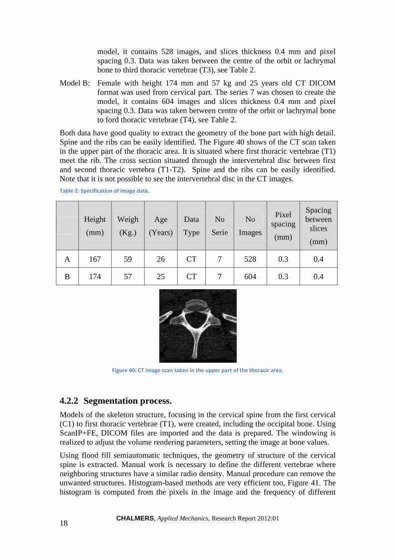
Both data have good quality to extract the geometry of the bone part with high detail.

Spine and the ribs can be easily identified. The Figure 40 shows of the CT scan taken

in the upper part of the thoracic area. It is situated where first thoracic vertebrae (T1)

meet the rib. The cross section situated through the intervertebral disc between first

and second thoracic vertebra (T1-T2). Spine and the ribs can be easily identified.

Note that it is not possible to see the intervertebral disc in the CT images.

Table 2: Specification of image data.

Height

(mm)

Weigh

(Kg.)

Age

(Years)

Data

Type

No

Serie

No

Images

Pixel

spacing

(mm)

Spacing

between

slices

(mm)

A 167 59 26 CT 7 528 0.3 0.4

B 174 57 25 CT 7 604 0.3 0.4

Figure 40: CT image scan taken in the upper part of the thoracic area.

4.2.2 Segmentation process.

Models of the skeleton structure, focusing in the cervical spine from the first cervical

(C1) to first thoracic vertebrae (T1), were created, including the occipital bone. Using

ScanIP+FE, DICOM files are imported and the data is prepared. The windowing is

realized to adjust the volume rendering parameters, setting the image at bone values.

Using flood fill semiautomatic techniques, the geometry of structure of the cervical

spine is extracted. Manual work is necessary to define the different vertebrae where

neighboring structures have a similar radio density. Manual procedure can remove the

unwanted structures. Histogram-based methods are very efficient too, Figure 41. The

histogram is computed from the pixels in the image and the frequency of different


19

parts. Peaks and valleys in the histogram are used to locate the clusters in the image

based in the color and the intensity.

Figure 41: Histogram, comparison between grey scale and number of pixel

Nine masks were created, one mask for each vertebra, including: First (C1), second

(C2), third (C3), fourth (C4), fifth (C5), sixth (C6), seventh (C7) cervical vertebrae,

the first thoracic vertebrae (T1) and the base of the occipital bone. Each mask of each

vertebra was defined in a different file. So it was possible to minimize the memory

used and reduces the computational time in the segmentation process. Morphological

filter and smoothing is applied in the masks. The same technique and values was used

for each mask and both models. Using Boolean operation, overlapping is avoided.

Also, 3D editing tools were using to smooth specific regions.

The same volume and topology are preserved with a focus on: the contact surface for

the intervertebral discs, the contact with nerves and the transverse foramen. Figure 42

shows an example of the seventh vertebrae, where the blue colour shows the regions

of interest where high anatomical accuracy is needed.

In addition, this project also checked the possibility of improving the model, adding

some soft tissues from the CT data. Automatic techniques are not very useful here,

manual work is necessary to extract the muscles. Figure 43 shows the

sternocleidomastoid muscle extracted from CT images data of Model A.

Figure 42: Same volume and topology are preserved. Example seventh cervical vertebrae.

Figure 43: Muscle extracted from CT model A


20

4.2.3 3D Analysis – Comparison of models

The geometries of the structure of two female necks were extracted. Figure 44 shows

the 3D view of the both models. The Model A has more curvature compared with the

Model B. Geometrical comparison of angles between vertebrae, spine curvature and

volume were performed.

Figure 44: Right model or Model A from female with height 167 mm and 59 kg and the left model or Model B from female with height 174 mm. and 57 Kg.

4.2.4 Comparing the angles of contacts surfaces

One of the targets for this project was to preserve the feature of the contact surfaces in

the vertebral joints. It was taken into consideration during the segmentation process.

The angle between the surfaces of the vertebrae is useful to evaluate how well the

spinal kinematics can be simulated. It was extracted in Table 3. The angles of the

surface between the vertebrae and the intervertebral discs are provided for both

models. The measures were taken from the 3D models, and it is provided with respect

to the horizontal plane.

The measure of the angles of model A and model B were compared. The data shows a

change in the measure of the angles between the first and second vertebrae cervical.

The third until seventh cervical vertebrae show similar measures. In addition, the

angle of the contact surface between the first and the second cervical vertebrae is

smaller compared with the other vertebrae. The model A shows more curvature

compared to the model B, it can be due to an extension of the neck during the

scanning.

Volume and moments of inertia were extracted for each vertebra; see Table 3. The

volume was taken as the total mask volume, treating each voxel within the mask as a

cuboid. The moments of inertia tensor measures assume that the material density is

constant. It is computed using the moment of inertia of a cuboid voxel. To recover the

true moment of inertia, the values must be multiplied by the material density.

The first and the seventh cervical vertebrae show a reduction of the volume between

the Model B compared to Model A of 30%. The third and the sixth cervical vertebrae

show a reduction of 20% and the other shows similar volumes. Some topology is lost

when the element mesh is reduced, so it introduces a change in the volume measure in

comparison with the real volume of the vertebrae. The small geometrical features are

more sensitive to an increase of the element size, regarding a change in the volume.


21

Table 3: Angles contacts surface vertebrae.

First Vertebrae Cervical (C1) – Atlas

A

(Degree)

B

(Degree)

Angle Inferior Left (αIL): 23 34

Angle Inferior right (αIR): 20 35

Second Vertebrae Cervical (C2) – Axis

A

(Degree)

B

(Degree)

Angle Superior Left (αSL): 22 32

Angle Superior right (αSR): 20 35



Third Vertebrae Cervical (C3)

A

(Degree)

B

(Degree)





Fourth Vertebrae Cervical (C4)

A

(Degree)

B

(Degree)






22

Fifth Vertebrae Cervical (C5)





Sixth Vertebrae Cervical (C6)





Seventh Vertebrae Cervical (C7)






23

Model A Moments of inertia (mm5)

Vol (mm3) Ixx Iyy Izz Ixy Ixz Iyz

C1 9.16e03 1.16 e06 2.91e96 3.69e06 163e03 114e03 260e03

C2 13.2e03 2.23e06 2.32e06 3.38e06 42,6e03 -14.0e03 369e03

C3 6.96e03 653e03 1.09e06 1.54e06 -42.6e03 16.4e03 14.6e03

C4 8.78e03 821e03 1.56e06 2.10e06 -66.5e03 32.2e03 24.5e03

C5 9.24e03 991e03 1.80e06 2.46e06 -101e03 63.9e03 13.7e03

C6 8.59e03 1.32e06 1.54e06 2.59e06 -2.10e03 33.8e03 -80.5e03

C7 10.3e03 1.87e06 2.03e06 3.49e06 -33.3e03 -23.1e03 -205e03

Model B Moments of inertia (mm5)

Vol (mm3) Ixx Iyy Izz Ixy Ixz Iyz

C1 12.4e03 1.75e06 4.82e06 6.21e06 279e03 -332e03 21.7e03

C2 14.7e03 2.62e06 2.60e06 4.14e06 -118e03 9.09e03 412e03

C3 9.14e03 900e03 1.53e06 2.17e06 -6.15e03 2.51e03 5.92e03

C4 9.07e03 870e03 1.65e06 2.21e06 23.6e03 15.6e03 18.6e03

C5 8.72 e03 690e03 1.92e06 2.38e06 -15.6e03 -8.65e03 37.8e03

C6 11.3e03 1.26e06 2.23e06 3.11e06 -43.0e03 -66.3e03 -78.5e03

C7 14.3e03 2.47e06 2.75e06 4.49e06 46.7e03 -68.2e03 -251e03

4.2.5 Finite Element mesh generation

FE models and CAD surface (STL file format) were generated with ScanIP+FE and

the FE mesh was imported directly to LS-Dyna. The mesh is exported with length unit

in millimetres. Much effort was put in analysing how to reduce the final number of

elements.

The mesh is generated using tetrahedral and hexahedral. Using adaptive meshing to

boundaries and interior elements setting with a large target value should reduce the

final number of elements. But in this project, it is interested has similar elements size

in the mesh. Figure 45 shows a relation between the number of elements and length of

the element edge. The main interest is to have a peak location around the mean length

edge element and a small deviation, see Figure 46, where it is shown in the graph with

a thick line. So, in this case, there are similar sizes in the elements of the mesh. To

reduce the computational time, the mean element edge length should be as high as

possible.


24

Figure 45: Relation between number of elements and length edge element mesh.

Figure 46: Relation between number of elements and length edge element mesh, thick line shows similar size of elements.

The numbers of pixels are directly linked with the number of elements after the

meshing process. So, another way to reduce the number of elements is to down

sample the data before meshing, but making sure that it does not lose the features that

are interesting to preserve. An analysis to choose the down sample value was realized,

evaluating the feature that it is losing when different values are used. Figure 47 shows

a graph where the number of elements in the mesh is compared to the reduction of the

volume. It is assumed that the 100% volume is in the case with the pixel value from

the data without any transformation. Hence, in this case it is possible to reduce the

number of elements by fifty per cent and still have the reduction of volume very low.

Figure 48 shows an example of when the number of element is reduced so much that

it is even changing the geometry of the model. In this example, the first vertebra from

the model A is showed. The ideal spacing has to be chosen depending on the size of

the smallest feature that should be captured in the model, see Figure 49. Based in this

analysis, the data is down sample with a 1.4 mm pixel size.

Figure 47: Relation between number elements in the mesh and volume.

Figure 48: Relation between number of elements and topology and volume that is reduced.

Figure 49: Small feature define mesh size.


25

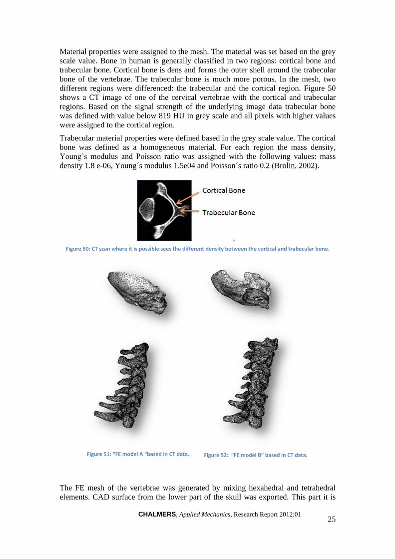
Material properties were assigned to the mesh. The material was set based on the grey

scale value. Bone in human is generally classified in two regions: cortical bone and

trabecular bone. Cortical bone is dens and forms the outer shell around the trabecular

bone of the vertebrae. The trabecular bone is much more porous. In the mesh, two

different regions were differenced: the trabecular and the cortical region. Figure 50

shows a CT image of one of the cervical vertebrae with the cortical and trabecular

regions. Based on the signal strength of the underlying image data trabecular bone

was defined with value below 819 HU in grey scale and all pixels with higher values

were assigned to the cortical region.

Trabecular material properties were defined based in the grey scale value. The cortical

bone was defined as a homogeneous material. For each region the mass density,

Young‟s modulus and Poisson ratio was assigned with the following values: mass

density 1.8 e-06, Young´s modulus 1.5e04 and Poisson´s ratio 0.2 (Brolin, 2002).

Figure 50: CT scan where it is possible sees the different density between the cortical and trabecular bone.

Figure 51: “FE model A “based in CT data.

Figure 52: “FE model B” based in CT data.

The FE mesh of the vertebrae was generated by mixing hexahedral and tetrahedral

elements. CAD surface from the lower part of the skull was exported. This part it is


26

useful to uses a reference for positioning the neck. In the preprocessing pre-smoothing

was applied and set with minimum edge length of 3 mm. and 7 mm. It was exported

using absolute global coordinates (base in the CT data) and STL format file and FE

model was exported to LS-Dyna. Same method was used for each vertebra and

applied to both models. The number of elements in model A is 18e04 elements

(Figure 51) and 16e04 model B (Figure 52). Based on the complex geometry of the

vertebrae, the 90% of the elements in the mesh are tetrahedral.

4.3 Conclusion

CT image of two female patients were used to create three dimensional FE models of

the cervical spine to analyze with the LS-Dyna software. Using image processing and

model generation techniques numerical models were created that followed the real

geometry with high detail. A model of the cervical spine was extracted, between first

cervical vertebrae (C1) until first thoracic vertebrae (T1) including the base of the

occipital bone.

The data used had good quality and it was possible to extract the geometry of the bone

with high detail. The bony parts can be easily identified and semiautomatic techniques

are very useful in this case. The volume and topology in specific regions of interest

were preserved. 3D editing tools made it possible to apply filters in specific regions.

Visual comparison between two models was easy using the 3D models.

In order to reduce the total number of elements, an analysis was performed. The aim

was to have similar sized elements in the meshes, so interior elements with large value

were not interesting in this case. Material properties base in the grey scale value are

possible to define, and different regions can be differentiated. The total number of

elements depends of the size and required detail of the model. The mesh was

generated with a mix of hexahedral and tetrahedral elements. The hexahedral

elements are often generated in the center of the vertebrae and the edges are

tetrahedral. Using image processing techniques is possible extract FE models with

high geometry detail and very close to the real. It is possible create a 3D model,

analysis the geometry and extracting measures.

In addition it is possible to generate numerical models and export directly to

commercial software, in this case LS-Dyna. The FE model is generated with

ScanIP+FE. There were some advantage and some limitations:

It is possible to extract a model that follows the geometry with high detail. But

with more detail and more complex geometries the total number of elements is

increased.

More data increase the time consumed in image process, so it is very important

work in small files keeping only the necessary data.

It is possible to generate tetrahedral and hexahedral meshes, but it lacks a high

control and flexibility in the mesh. It would be good to have a manual tool to

change the elements of the mesh in specific regions.

The center of mass is given directly according with the local reference system;

it would be good to get the center of mass according to the global reference

system.

It is possible extract some muscle geometry from the CT data but manual work

is required.


27

It is concluded that image processing is useful tool to create FE models to evaluate the

cervical injury.

4.4 Future work

The models can be improving by adding the intervertebral disc, spinal cord or/and

spinal nerves, see Figure 53 and Figure 54. It is not possible to extract information

about these tissues from the available CT data. However, there are several options:

Using other set of CT data or MRI data where the intervertebral disc and soft

tissues can be extracted, or

to generate the geometry based on data from the literature, or

to assume that the space between the vertebrae is filled by the intervertebral

disc.

In addition the model can be improved adding soft tissue. Some soft tissue can extract

from the CT but from MRI or literature they can generated with more detail, Figure

55.

Figure 54: spine cord or / and spine nerve.

Figure 55: Sternocleidomastoid muscle.

Figure 53: Intervertebral disc.


28

5 Animals Models Project

Traumatic brain injuries (TBI) are one of the major public health problems in all parts

of the world. The consequences following these injuries are serious and frequently

present throughout life. Animal experiments, to serve as human surrogates, have been

regarded the main possibility in the studies of brain injury mechanisms in the past.

In this project, image processing was used to support the development process of

animal head and neck numerical models. One rat and one monkey FE model were

developed. The models are being used to simulate recent rat experiments, Davidsson

(2011) and monkey experiments carried out in the past, Ono (1980).

The image processing tasks presented here were developed within the frame of the

collaborative research in head injuries between Chalmers and the Japan Automobile

Research Institute (JARI). Ermes Tarallo from Politecnico di Milano, Jacobo Antona

Makoshi, from JARI and Chalmers, and Johan Davidsson from Chalmers were

involved in this part of the project.

5.1 Rat project

5.1.1 Background

The main interest of this current project is to extract the geometry of the scalp and

skull for two rats with different mass. Comparisons of both specimens were realized

and one specimen was chosen for the FE model generation. The model was simplified

in some regions for the simulation, preserving details only in the regions of interest.

Also, the spine was extracted and added to the model.

This project is focusing in image processing. The geometry was extracted using

ScanIP+FE Simpleware software.

5.1.2 Work process

CT images, on DICOM format, of two specimens were used to create CAD surface

models of the skull, the scalp and the cervical spine. The data was extracted from two

male rats with mass of 290 and 640 grams, respectively. The data was provided by the

Karolinska Institute, Stockholm, on September 29th

, 2011. The images were taken in

accordance with the Swedish National Guidelines for Animal Experiments, which was

approved by the Animal Care and Use Ethics Committee in either Umeå or

Stockholm.

5.1.2.1 Data

Rat_290: The data of the male rat with 290 grams mass was created based on the

series no 5, where 885 slices images were acquired from the seventh

cervical vertebra to the skull, with spacing size 0.078 mm (Table 4).

Rat_640: The data of the male rat with 640 grams mass was created based on the

series no 13, where 1014 slices images were acquired from the sixth

cervical vertebrae to the skull, with spacing size 0.078 mm (Table 4).


29

Table 4: Specification of the data.

Data

type

No

Series

Weight

(Grs) Gender

No

Images

Spacing

size

(mm.)

Rat_290 CT 5 290 Male 885 0.078

Rat_640 CT 13 640 Male 1014 0.078

5.1.2.2 Segmentation process – skull and brain cavity

Segmentation of the skull of the both specimens was realized to extract the

geometrical dimensions of the skull and brain cavity and a comparison of the two

specimens was realized. The same methodology was applied for both models.

Figure 56 shows a CT image of a rat head, the cross section was taken from the

horizontal plane. The bone can be easily identified; the image shows the skull and the

mandibular bone. The grey scale with lower value is the skin. However, with the CT

data it is not possible distinguish any soft tissue inside the skull. It is possible to

extract the brain cavity. This can be combined with the literature (such as an

anatomical atlas) to extract the brain geometry (or combine with other data, such as

MRI).

The memory required to process the data is very high so it was necessary crop the

data. The background used for segmentation of bones was set to double pixel value.

Semiautomatic methods based on the grey scale value, such as threshold and flood

fill, were applied to segment the regions of interest and create the mask. And manual

tools were necessary to use. Two masks were created: brain cavity and skull mask, see

Figure 57. Morphological filter were applied in the Skull mask. 3D editing tools in

front region of the skull was used to simplify this region that it is not necessary high

geometric detail. The 3D models of the skull are shown in Figure 58 and Figure 59.

Boolean operations were used to create the brain cavity mask based in Skull mask.

The 3D models of the brain cavity of both specimens are shown in Figure 60 and

Figure 61.

Figure 56: CT scan image of a rat head

Figure 57: Two mask: Skull and Brain cavity

.


30

Figure 58: 3D Model of the skull based on CT data Rat_290

Figure 59: 3D Model of the skull based on CT data Rat_640

Figure 60: 3D Model of the brain cavity based on CT data Rat_290

Figure 61: 3D Model of the brain cavity based on CT data Rat_640

5.1.2.3 Segmentation process – Scalp

The scalp of both specimens is extracted. The background used for the segmentation

was set with double pixel value. Semiautomatic tool such as threshold was applied to

segment the regions of the skin and the skin mask was created. Figure 62 shows the

3D models with the scalp, skull and brain cavity.

Figure 62: 3D models with the scalp, skull and brain cavity. Model in the right belong data from RAT 640 and left model belong to data specimen RAT 290.

5.1.2.4 3D Analysis – Comparison models

Both specimens were compared. The Figure 63 shows orthogonal view of the models

with the scalp, skull and brain cavity of both specimens. Measures were extracted

from the models for the comparison using ScanIP+FE: volumes, density grey scale,

centre of mass, inertia properties and the main measure of the skull.


31

The volumes of the both models were measured. The volume in millimeters cubic

(mm3) and it is provided the total mask volume, treating each voxel within the mask

as a cuboid. For Rat 290 grs, the volume of the skull mask was 3.37e3 and 1.85e3

mm3 for the Brain Cavity mask. The mean grey scale of the skull masks 2.18e3, see

Table 5. And in the Rat 640 grs, the volume of the skull mask was 5.42e3 and 2.31e3

mm3 for the brain cavity mask. The mean grey scale of the Skull masks 2.23e3, see

Table 5.

Table 5: Volume skull and brain cavity mask of the rat models.

Skull mask

Volume (mm3)

Brain cavity

Volume (mm3)

Rat_290GRS 3.37e03 1.85e03

Rat_640GRS 5.42e03 2.31e03

The maxims measure of the skull and the brain cavity based in the reference system of

the CT scan data were extracted according with Figure 64. The moment‟s inertia and

centre of mass of the skull and brain cavity mask were extracted. These measures

were calculated with ScanIP+FE, based in the local reference system from the CT

image data, Table 6.

Using ScanIP+FE the measure of the centre of mass of the mask is extracted base in

the local reference system of the CT image. Anyway it is possible change of

coordinates from one to another reference system. Based on that we know both

reference system and we can easily transformation coordinate of the point local

reference system of the CT image to another reference system or in the opposite way,

global to local. This is an easy method but need time, and based in the limited time of

the project it was provided the centre of the mass of the masks in local reference

system.

Figure 63: lateral and top view of the Rat models created based in CT data. Right model was created based in data Rat 640 grs; left model was created based in data Rat 290.


32

The center of mass of the mask is provided the three coordinates directions (X, Y, Z)

in millimeters (mm). Each voxel is assumed to have identical mass. The moments of

inertia tensor for the mass assume the material density is constant. It is computed

using the moment of inertia of a cuboid voxel. To recover true moment of inertia, the

values must be multiplied by material density.

Measure Skull and brain cavity (mm)

Xmax Ymax Zmax Xmax_Cerebl Ymax_Cerebl Zmax ()

Skull_Rat_290 21 21 44 X X X

Skull_Rat_640 27 26 56 X X X

BrainCavity_Rat_290 15 10 23 5 4 19

BrainCavity_Rat_640 15 10 27 4 4 23

Figure 64: Max. Dimensions Skull and Brain cavity from Rat 290 grs and Rat 640 grs.


33

Table 6: Centre of Gravity and Moments inertia based in the reference system of the CT image data.

Centre Mass L

(mm) Moments Inertia Tensor (mm5)

x y z Ixx Iyy Izz Ixy Ixz Iyz

Skull_Rat_290 12 10 21 5.1e05 4.9e05 1.7e05 -1.1e04 -2.5e04 -3.1e04

Skull_Rat_640 15 13 27 1.2e06 1.1e06 4.1e05 -3.4e04 -9.1e04 -1.4e05

BCavit_Rat_290 11 6 11 6.5e04 7.3e04 3.1e04 6.6e02 -2.2e03 6.6e03

BCavit_Rat_640 13 8 14 1.0e05 1.1e05 4.2e04 3.1e03 -3.1e03 2.9e03

The measure of the skull from both specimens was extracted based on the centre of

mass of the Brain Cavity. Based in this centre of mass of the Brain cavity mass lines

in the direction of the three axles and their diagonal were generated. The intersection

of these lines with the skull and scalp give the measure of the diploe table in, diploe

table out and scalp. It is showed in the graphs Table 7. The measures were extracted

in millimetres.

Based in the result of the skull and brain cavity; the skull model from Rat 640

presents 110 % of volume bigger than the model from data Rat 290grs. Instead the

brain cavity shows a change in the longitudinal measure (according direction axle Z)

between both specimens. But the brain cavity does not change its dimension lateral

and vertical direction (according axle X and Y).


34

Table 7: Thickness skull and scalp

0

10

20

RAT MALE 290- XY

0

10

20

RAT MALE 640- XY

0

10

20

RAT MALE 290- ZY

0

10

20

RAT MALE 640- ZY

0

10

20

RAT MALE 290- XZ

0

10

20

RAT MALE 640- XZ


35

5.1.2.5 Segmentation process

Based on the results of the comparison the specimen Rat 640 grs was chosen and

complete analysis is performed in one specimen. The skull was simply for the

simulation, with the exception of same specific regions. The Figure 65 shows a cross

section view of the skull of the Rat 640 grs, where it is specify what parts need to

preserve intact.

The region preserved was: the internal cavity, condyles occipitals and the foramen

magnum and the upper surface of the skull, these parts were kept almost intact, the

Figure 65. The cavities of the skull were filled applying filters and the rest of the skull

smoother using 3D editing tools.

Figure 65: Skull of a Rat, where shows same topology that was necessary preserve.

The cervical were extracted, from first (C1) until sixth cervical vertebrae (C6) were

segmented. Based in region growing techniques and flood fill tools, the regions of

interest were segmented. Six masks were created, one mask for each vertebra: First

cervical vertebrae (C1), second cervical vertebrae (C2), third cervical vertebrae (C3),

fourth cervical vertebrae (C4), fifth cervical vertebrae (C5) and sixth cervical

vertebrae (C6), see Figure 66.

Figure 66: Anatomy of the cervical vertebrae from C1 to C6 and Skull.

Morphological filters and Gaussian were applied in each mask to fill the cavity. The

same method was realized for each vertebra. Boolean operations were used to avoid

overlapping between the vertebrae Figure 69.

The skull was simplified using 3D editing tools. For the simplification was taken

account that same topology and volume had to be preserved. The Figure 67 shows the

skull before the simplification and the Figure 68 shows the skull after simplification.


36

Figure 67: 3D model of the skull from data Rat 640 grs.

Figure 68: 3D model of the skull from data Rat 640 grs simplified.

5.1.2.6 CAD Surface generation

Surface tetrahedral mesh models of skull and brain cavity from Rat 290 grs and Rat

640 grs were generated (models before the simplification). Target minimum and

maximum edge length was defined in 0.3 and 0.8 mm. respectively. In addition pre-

smooth in the generation of the mesh was applied. It was exported in STL file format.

Surface tetrahedral mesh model of skull simplified, brain cavity and the cervical neck

between first to sixth cervical vertebras (C1-C6) were generated. Target minimum and

maximum edge length were defined in 0.3 and 0.8 mm respectively. In addition pre-

smooth in the generation of the mesh was applied. It was exported in STL file format.

The Figure 69 shows the CAD surface of the skull simplified and Figure 70 shows the

brain cavity from data RAT 640 grs.

Figure 69: CAD surface of the skull simplified from data Rat 640 grs.

Figure 70: CAD surface of the brain cavity from data Rat 640 grs.

The volume and inertia properties of the Skull simplified, brain cavity and neck (C1 to

C6) were extracted, see Table 8. The volume in millimeters cubic (mm3) and it is

provided the total mask volume, treating each voxel within the mask as a cuboid.

The inertia properties and centre of mass of the skull simplified, brain cavity and neck

masks were extracted. These measures were calculated with ScanIP+FE, based in the

local. The moments of inertia tensor for the mass assume the material density is

constant. It is computed using the moment of inertia of a cuboid voxel. To recover

true moment of inertia, the values must be multiplied by material density.


37

Table 8: Inertia properties and volume from Male 640 grs of the skull simplified, brain cavity, neck and skin.

Moments Inertia (mm

5) Volume

(mm3) Ixx Iyy Izz Ixy Ixz Iyz

Skull_R640

Simplified 1.8e06 1.8e06 5.6e05 -3.3e04 -1.1e05 -1.5e05 8.8e03

Brain

cavity_R640 1.0e05 1.1e05 4.2e04 3.1e03 -3.1e03 2.9e03 2.3e03

C1_R640 8.1e02 2.4e03 2.7e03 4.3e02 4.9e01 -1.5e02 1.4e02

C2_R640 1.9e03 1.6e03 1.1e03 -2.1e01 -6.6e01 -6.2e02 1.3e02

C3_R640 3.8e02 6.8e02 5.9e02 4.8 e01 -3.2e01 -8.8e01 8.0e01

C4_R640 3.5e02 8.9e02 9.1e02 9.6 e01 -2.4e01 -6.2e01 8.7e01

C5_R640 2.8e02 6.9e02 7.6e02 8.9 e01 -3.1e01 -4.7e01 7.5e01

C6_R640 5.3e02 1.3e02 1.5e02 6.9e01 -7.6e01 5.0e01 1.1e02

5.2 Monkey project

5.2.1 Background

This research project is conducted by Jacobo Antona Makoshi from JARI and

Chalmers. The main interest of the current project is extracted the geometry of the

skull and cervical from two monkeys from different data. Two CT scan data were

acquired from two male monkeys to create one model. The images from the first

specimen (MFF2115) were taken in accordance with the Kyoto University Primate

Research Institute (KUPRI) Ethics Committee in Japan. The purpose of the use of the

images was specified through a collaboration agreement between JARI and KUPRI.

The images from the second specimen (Mff1761) were downloaded from the KUPRI

online morphology museum.

The alignments of the neck of the model did not correspond with the posture of the

neck of the experiments to be simulated, see Figure 71 a). Hence, it was necessary to

add the cervical spine from another CT set with the correct alienation. So the

geometry of the skull and the spine were extracted from different specimens and

aligned in the correct posture according with the experiments, Figure 71 b).

a) b)

Figure 71: Monkey model based in two different data. A) The spine for the simulation it is not in the position that is required for the simulation. B) Data from the spine from other specimen was aligning with the current model.


38

5.2.2 Work process

CT DICOM image of two specimens were used to create a CAD surface model of

skull, scalp and cervical spine. The data was extracted from two male monkeys from

two different data sets to create one model. The segmentation and meshing process of

the skull and scalp of specimen MFF2115 was realized by Jacobo Antona Makoshi.

The cervical neck segmentation and alignment tasks were carried out by Marta

González Carcedo.

5.2.2.1 Data

Model A: CT DICOM data acquired from the head and neck with the specimen

MFF2115 in prone position, until fifth cervical vertebrae (C5). Data used

is from series 4. It has 680 images with pixel size 0.25 mm and spacing

between slices is 0.2 mm. see Table 9.

Model B: CT DICOM data acquired from the head and neck with the specimen

Mff1761 in supine position, until fifth cervical vertebrae (C5). Series 15

is the data used. It has 721 images with pixel size 0.31 mm and spacing

between slices is 0.2 mm. see Table 9.

Table 9: Information data used to create the models.

Specimen Data

type

No.

Series

No.

Images

Pixel

size

(mm)

Spacing

between

slices

(mm)

Model A MFF2115 CT 4 680 0.25 0.2

Model B Mff1761 CT 15 721 0.31 0.2

5.2.2.2 Segmentation process

Based in the previously extracted skull model, this current project tries to add to the

model a cervical neck with the right alignment. It was necessary to do:

a) Fast segmentation of the skull and first cervical of Model A, Figure 72a.

b) Segmentation of base of the skull and cervical vertebrae Model B, Figure 72b.

c) Positioning the Model B based in Model A, and generate CAD surface of the

vertebrae, Figure 72c.

(a) (b) (c)

Figure 72: Segmentation process of the Monkey model. a) Fast segmentation skull and C1 model from CT data Model A; b) Segmentation base of the skull and neck from CT data Model B; c) Align the models and generate CAD surface.


39

The research starts importing the data of specimen Model A to ScanIP+FE. A fast

segmentation of the skull and the first cervical vertebrae (C1) was realized from scan

data Model A. This segmentation is used as a reference to align the neck.

Figure 73: Anatomy of the first cervical (C1) vertebrae and Skull

The data from Model B was imported to ScanIP+FE. And the segmentation of the

cervical neck between first to fifth cervical vertebrae (C1-C5) was realized. In

addition a fast segmentation of the skull base was realized. Flood fill tool was used for

the segmentation process. Six masks was created, one mask for each vertebrae: first

cervical vertebrae (C1), second cervical vertebrae (C2), third cervical vertebrae (C3),

forth cervical vertebrae (C4), fifth cervical vertebrae (C5) and base skull.

Morphological filter and smooth were applied in the masks to reduce the noise. And

Boolean operation was used to avoid overlapping.

Figure 74: Anatomy of the cervical vertebrae from first cervical (C1) to fifth cervical vertebrae (C5) and base Skull

After the segmentation was realized, it was aligned with ScanIP+CAD to create one

model. But it was necessary have the same spacing than the data Model A. So the new

pixel value is 0.5 mm and slices thickness 0.4.

5.2.2.3 CAD surface generation

CAD surface of the skull and first vertebrae from specimen Model A and skull and

neck from Model B were generated. Using the ScanIP+CAD module was possible

imported and positioned the neck from Model B with the skull Model A. The model

was align taken the reference the centre of mass of the first cervical vertebras and the

occipitotlantal joint on the skull base. When the model has been positioned, the

project was exported back to ScanIP+FE to check the position with the CT data and

prepare the surface. And CAD surface was generated from the neck of Model B and


40

exported as are reference system base in Model A, see Figure 75. The mesh was

realized with other software.

Figure 75: CAD Surface of the spinal neck from CT data of Specimen Model B was positioning according with the skull generated based in CT data of Specimen Model A.

5.3 Conclusion and future work

Based in RAT project, CT DICOM image of two specimens were used to create a

CAD surface model of skull, scalp and cervical spine. It is possible extract the

geometry of the bones and the scalp with high detail. In addition it is possible

simplified specific region for the FE analysis.

It was not possible extract the anatomy of the brain based in the CT images provided.

It can be combining with other techniques, like using other set of CT or MRI images

or literature information (atlas), the model can develop adding information of the

anatomical part of the rat brain soft tissue.

More detailed anatomical analysis can be realized using more specimens.

For the monkey model project, CT DICOM image of two specimens were used to

create a CAD surface model of skull, scalp and cervical spine. The segmentation and

meshing process of the skull and scalp was done based on one specimens which

images were taken in supine position, while the tasks presented here consisted on

adding and aligning the neck taken from a data set obtained in prone position.

CAD surface from the neck was extracted from CT data. It was aligned with the skull

and the scalp of a model generated from another CT scan data.

So the result is based in two different data it is possible to segment, positioning and

generates a model. Being possible improve another models adding information from

different fonts. And in the same way than the rat model, using other techniques the

model can be develop adding information of the anatomical part of the rat brain soft

tissue.


41

6 Workshop

This project ended with a workshop with focus on how to generate numerical models

for simulation based on medical imaging. It presented the status regarding methods to

go from CT and MRI to FE and CFD models. The workshop included presentation

and hand-on exercises.

6.1 Contents

The workshop was a week programme; it was realized between Monday 12th

to Friday

16th

of December, 2011. It was located at the SAFER vehicle and traffic safety centre

at Chalmers, Göteborg. It started with an introduction about why and how this project

was carried out, followed by a presentation about the methodology of model

generation and the three applications. The workshop included a hand-on exercises and

a final discussion. The programme was distributed in three topics, as explained in

more detail below:

- Initial presentation (Section 6.1.1),

- Hand-on exercise during the week (Section 6.1.2),

- Final presentation (Section 6.1.3).

6.1.1 Initial presentation

The initial presentation took place on Monday 12th

December. Approximately 20

people participated at this initial presentation. During the presentation and after, a

group discussion turned on, so the presentation was very interactive and the

participants were very active and showed much interest.

10:00-12:00

The workshop started at 10.00 pm with introduction to the Human Body

Modelling group at Applied Mechanics and why and how this project was

carried out. It was presented by Karin Brolin.

Following a short introduction and presentation about medical imaging,

focusing in the methodology to go from the scan data to generate a numerical

model was presented by Marta Gonzalez Carcedo. This presentation had

duration of 15 minutes with same time for the questions.

A presentation of the methodology from image processing to validation of the

model, focusing in the model generation on animals brain models, presented

by Jacobo Antona Makoshi from JARI and Chalmers. The presentation and

the questions had duration of 35 minute.

Following presentation of three different applications, which are including in

this project, was presented by Marta Gonzalez Carcedo. This presentation had

duration of 25 minutes with same time for the questions.

12.00-12.30 h/ 13.00-14.30

It was expected to finish with the presentations before lunch. However, the

time for the questions was not enough so it was necessary to continue after

lunch with the presentation workflow process on how to generate models. An

introduction in ScanIP+FE Simpleware software was realized, giving the

participants a tutorial on how they could start to work with the software.


42

Presentation of workflow about the image process and model generation was

carried out by Marta Gonzalez.

6.1.2 Hand-on exercise during the week

Hand-on exercise during the week was taken place between Monday 12th to Friday

16th December. The participants got a short term license for the Simpleware software

to install on their own computer and the Division of Vehicle Safety (Applied

Mechanics department of Chalmers) provided computers for those if needed. In

addition, places to sit were available at SAFER for all participants. The participants

were free to show up whenever they could.

Approximately 10 people participated in the hands-on exercises. Marta Gonzalez

Carcedo was supporting the participants full time together with Jacobo Antona

Makoshi. Instructions for the installation process were provided the participants. The

participants could work in examples following tutorials and/or with their own data.

6.1.3 Final presentation

Final presentation was taken place on Friday 16th December. The workshop ended

having a discussion the experience of the workshop week and discussion on how to

generate models from medical imaging in the future. This workshop was moderated

by Karin Brolin and during 2 hours the participants presented their results and

discussed their experiences.

10:00-12:00

The workshop starting with a summary about what the experiences learned

during the week. Following a summary and group discussion on the usability

of image processing method was realized and pros and cons of the software. It

ended by having a discussion on how to generate models from medical

imaging in the future.

6.2 Hand-on Applications

The workshop participants were researchers from different areas such as fluid

dynamics, medicine, and vehicle safety. It was great to exchange knowledge and

experience from the point of view of the different fields. Approximately 10 people

participated in the hands-on exercises. Marta Gonzalez Carcedo was supporting the

participants full time together with Jacobo Antona Makoshi.

Below is a summary of applications which the participants working on during:

Modeling of stent graft of the aorta based on CT data form CFD analysis by

Håkan Nilsson from Chalmers, Håkan Roos from Sahlgrenska University

Hospital.

Skeleton structure of the neck from females based in CT data for FE analysis

by Karin Brolin from Chalmers, focusing in evaluation of the influence in

spinal kinematics.

Skeleton structure and soft tissue of the cervical spine based on CT data by

Jonas Östh from Chalmers.

Image processing of the shoulder based in CT data by Manuel Mendoza-

Vazquez from Chalmers.


43

Skeleton structure focusing on lower extremities of the several subjects based

on CT data for anthropometric analysis by Krystoffer Mroz from Autoliv.

Image processing of the tumor in the brain based in MRI data by Gayatri

Mirajkar Sonavane.

Application in material properties using image processing by Håkan Johansson

from Chalmers.

Instructions for the installation process were provided the participants the Friday

before the workshop. The participants could install the software before and everything

was ready on Monday for the workshop. Whose participants that they need help with

the installation software was helped on Monday for the supports.

The participants got a two weeks short term license of the Simpleware software to

install in their own computers. So the participants could work in SAFER and/or in

their own place. The licenses were kindly provided by Simpleware Ltd.

The Division of Vehicle Safety provided a computer with Simpleware license

installed for a person that needed computer. In addition, places to sit were arranged

for three persons that did not have a desk at the SAFER office. The participants were

free to show up whenever they could.

Every day, around three to four people were working with the software. The

participants started with examples following tutorials, after this first contact with the

software the participants started work with their own data. The first days less

questions showed up but after this day the participants asked a lot of questions.

Below same of the example result of this week workshop:

- Sternocleidomastoid muscle was extracted from CT-scan data by Jonas Östh,

PhD student from Active Human Body Model (AHBM) Chalmers, see Figure

76.

- CFD Model of Aorta Stent graft and aneurysm dilatation were generated based

in CT-scan by Håkan Nilsson from Chalmers, see Figure 77 and Figure 78.

- A steady flow in an aortic aneurysm based in CFD model generated with

Simpleware. It was generated the model and run with OpenFOAM by Håkan

Nilsson during the workshop, Figure 79.


44

Figure 76: Sternocleidomastoid muscle geometry derived from CT-scan during the workshop from Jonas Östh.

Figure 77: CFD Model of Stent graft generated derived from CT-scan during the workshop from

Håkan Nilsson.

Figure 78: CFD Model of Aortic aneurysm generated derived from CT-scan during the

workshop from Håkan Nilsson.

Figure 79: Steady flow in an aortic aneurysm. The CFD model was generated with Simpleware and simulation was run with OpenFOAM by Håkan Nilsson during the workshop.


45

6.2.1 Active Human Body Models project: Applications for medical

image processing

The following text was authored by Jonas Östh, PhD student in the Injury Prevention

group, Applied Mechanics, Chalmers University of Technology.

The aim of the Active Human Body Model (AHBM) project is to incorporate active

muscle responses in a human full-body Finite Element (FE) model, enabling the use

of an FE HBM to predict pre-crash kinematics and restraint interactions as well as

injury due to crash loading.

Currently in the AHBM project, muscle function is modelled using a simplified

approach with line elements that capture the muscle line of action, see Figure 80. For

this, anatomical literature provides a sufficient means to implement the muscles. One

possible further refinement of the model is to represent the muscle using solid

elements. To do this, there are two major requirements:

First a continuum muscle model that can represent the mechanical muscle properties

using solid elements (Khodaei and Mostofizadeh, 2010).

Second, a correct representation of the volume that the muscles occupy is needed.

To generate such geometries, medical image processing is a suitable approach. During

the medical imaging workshop the outline of the sternocleidomastoid muscle was

extracted from a set of CT-scan data, see Figure 81.

Figure 80: Musculoskeletal structure of the AHBM (Östh, 2010).

Figure 81: Sternocleidomastoid muscle geometry derived from CT-scan during the workshop from Jonas Östh.


46

6.2.2 Injury-HBM project

The following text was authored by Manuel Mendoza-Vazquez, PhD student in the

Injury Prevention group, Applied Mechanics, Chalmers University of Technology:

The objective of the injury human body model (I-HBM) project is to improve the

thoracic injury capabilities of a human body model. Restraint systems can be then

improved by evaluating and designing them using a human body model with better

injury prediction.

At this moment, the I-HBM project is focusing on improving rib fracture prediction.

There are several parameters that influence the mechanical response of the ribs and

their fracture. Bone material properties and geometry are among those parameters.

Medical imaging is an essential tool in defining rib geometry and material parameters.

The geometry parameters that can be defined are the rib cortical thickness, rib

transversal area and rib shape. The bone mineral density can be calculated with help

of medical imaging and this value can be then used to define the adequate material

properties.

It is known that the ribcage shape changes with age and that there are some

differences in the size of ribs between males and females. The effect of these changes

on the rib injury outcome is not completely understood yet. Human body models of

different populations could be a way to gain understanding about the effect of these

changes on rib injury outcome. A description of rib and ribcage geometries is a first

step to create human body models representative of different demographic groups.

Processing CT scans seems as a promising way to obtain representative geometries

for different populations.

During the workshop, I have evaluated the feasibility to automatically retrieve ribcage

geometries from CT scans using Scan IP. The conclusion was that the user still needs

to spend some time to retrieve the geometry and that the process cannot be completely

automatic yet.

6.3 Feedback

Approximately 20 people participated at the initial presentations; approximately 10

people participated in the hands-on exercises and the final workshop discussion.

These bullets below are a summary of the feedback given by the participants after the

final workshop discussion.

6.4 What did you learn?

That it is possible to create 3D models and export to other software.

Possibilities and limitations with the software.

To create 3D models from human medical data.

Software is user-friendly and can be implemented.

Did some tutorials and worked with CT-data, learned that time is needed to

learn the software and chose appropriate filters.

How medical images look like, are generated, and modified.

Filtering techniques for images and geometrical comparisons

Anatomical in own field and others


47

Unstructured mesh generation with tetrahedral

Deeper understanding of the status regarding methods to go from CT/MRI to

FE models

Valuable insight how the software works.

6.5 Value of the workshop?

Good orientation on how model generation based on medical images is done.

Knowledge about other projects at Chalmers.

Gave many ideas on how to use the software for other projects.

Useful from my research point of view and interesting.

Important to listen to other possible applications.

A good opportunity to get experience in the field.

Produced images that can be of value for marketing of research short and long

term.

Useful to be able to evaluate presented models and models made by others.

6.6 Feedback on the program/planning.

Good with initial presentations, individual work where we could get help and a

sum up in the end to exchange knowledge and experience.

Good format: rather short, focused but with room for discussions.

Good planning of the workshop.

The seminar form was good, with two hour intro and free work followed by a

summary.

Good that the software could be installed on own computer and worked with

during the week when time was available.

Marta helped and followed up the work of the participants in a good way.

It was great having Marta as an expert that worked with the software before

the workshop.

6.7 Conclusions

Below there are some of the pros and the cons of using image processing techniques

for model generation. It was extracted from the discussion of the participants in the

last day of the Workshop.

+ Image processing is a useful tool to identify geometries from images.

+ Good for measuring anatomical differences in different persons.

+ Can be used to create a 3D anatomical book for education use.

+ Good thing of using the Simpleware software, it has a good support from the

software company.

+ Useful tool to model generation

- Limited meshing

- Automatic tools are available but manual work is necessary.


48

6.8 Lesson learned

The main interest was to get knowledge about image processing giving in the

presentation time, adding with experience during the workshop week. The participants

were register giving some information about background and why they were

interested. So it helped to know what type of presentation and application would be

presented.

The licenses were given to the participants the week before, so they could install the

software before to be ready the first day of the workshop. In addition it was possible

use your own computer and work with during the week when time was available, so it

gave flexibility and compatibility with your schedule work.

The workshop week programmed was enough to have a first contact with the

software. It gave a great opportunity to get experience with image processing

methods. The time allocated for presentation was not enough; the discussion time was

longer that it was planned. Better workflow after lunch and have more time for

discussion.

Everybody that participates in the workshop was very interested in the field, with an

active participation and involving in the project. It made a nice and confidence

environment for the workshop, making easy the discussion and the workflow of the

workshop. The participants were from different areas, it helps to give a good

opportunity to exchange knowledge.


49

7 References

Davidsson J., Risling M., (2011): A New Model to Produce Sagittal Plane Rotational

Induced Diffuse Axonal Injuries. Frontiers of Neurotrauma, 2 (41) pp.1-11.

Ellis H., Logan BM., Dixon A. (2007): Human sectional anatomy: Atlas of body

sections, CT and MRI images. 3rd edition. London: Ed. Hodder Arnold.

Karin Brolin (2002): Cervical Spine Injuries – Numerical Analyses and Statistical

Survey. Ph.D. Thesis. Department of Aeronautics, Royal Institute of Technology.

Report 2002-29, Stockholm, Sweden.

Khodaei H, Mostofizadeh S. (2010): Continuum Models of Active Musculature for

Impact Biomechanics Simulation. Department of Applied Mechanics, Chalmers

University of Technology, Research Report no 2010:06, Göteborg, Sweden.

KUPRI - Kyoto University Primate Research Institute. Online morphology museum:

http://www.pri.kyoto-u.ac.jp/dmm/WebGallery/index.html (2012-01-20).

Marta González Carcedo (2010): Anthropometric Characterization of Human

Subjects. Department of Applied Mechanics, Chalmers University of Technology,

Publication no. 2010:53, Göteborg, Sweden.

Andersson P., Pilqvist J. (2011): Fluid-Structure Interaction analysis of the forces

causing stent graft migration. Department of Applied Mechanics, Chalmers

University of Technology, Publication no. 2011:23, Göteborg, Sweden.

SIMPLEWARE LTD (2011): ScanIP+FE+CAD Reference Guide. Exeter, United

Kingdom.

SIMPLEWARE LTD (2011): ScanIP+FE+CAD Tutorial Guide. Exeter, United

Kingdom.

Jonas Östh (2010): Active Muscle Responses in a Finite Element Human Body Model

[Licentiate thesis]. Chalmers University of Technology, Göteborg, Sweden.

Ono et al., (1980): Human Head Tolerance to Sagittal Impact - Reliable Estimation

Deduced from Experimental Head Injury Using Primates and Human Cadaver

Skulls. 24th Stapp Car Crash Conference, SAE 801303.

http://www.pri.kyoto-u.ac.jp/dmm/WebGallery/index.html


50

8 Appendices

This is the invitation for the workshop.

Publication link: http://www.chalmers.se/safer/EN/news/events/workshop-on-medical

http://www.chalmers.se/safer/EN/news/events/workshop-on-medical

Documents

Generation of numerical human models based on …publications.lib.chalmers.se/records/fulltext/local_155348.pdf · Generation of numerical human models based on medical imaging