Embed Size (px)
Citation preview
Generative Image Modeling using Style andStructure Adversarial Networks
Xiaolong Wang, Abhinav Gupta
Robotics Institute, Carnegie Mellon University
Abstract. Current generative frameworks use end-to-end learning andgenerate images by sampling from uniform noise distribution. However,these approaches ignore the most basic principle of image formation: im-ages are product of: (a) Structure: the underlying 3D model; (b) Style:the texture mapped onto structure. In this paper, we factorize the imagegeneration process and propose Style and Structure Generative Adversar-ial Network (S2-GAN). Our S2-GAN has two components: the Structure-GAN generates a surface normal map; the Style-GAN takes the surfacenormal map as input and generates the 2D image. Apart from a real vs.generated loss function, we use an additional loss with computed surfacenormals from generated images. The two GANs are first trained inde-pendently, and then merged together via joint learning. We show ourS2-GAN model is interpretable, generates more realistic images and canbe used to learn unsupervised RGBD representations.
1 Introduction
Unsupervised learning of visual representations is one of the most fundamentalproblems in computer vision. There are two common approaches for unsuper-vised learning: (a) using a discriminative framework with auxiliary tasks wheresupervision comes for free, such as context prediction [1,2] or temporal embed-ding [3,4,5,6,7,8]; (b) using a generative framework where the underlying model iscompositional and attempts to generate realistic images [9,10,11,12]. The under-lying hypothesis of the generative framework is that if the model is good enoughto generate novel and realistic images, it should be a good representation for vi-sion tasks as well. Most of these generative frameworks use end-to-end learningto generate RGB images from control parameters (z also called noise since itis sampled from a uniform distribution). Recently, some impressive results [13]have been shown on restrictive domains such as faces and bedrooms.
However, these approaches ignore one of the most basic underlying prin-ciples of image formation. Images are a product of two separate phenomena:Structure: this encodes the underlying geometry of the scene. It refers to theunderlying mesh, voxel representation etc. Style: this encodes the texture on theobjects and the illumination. In this paper, we build upon this IM101 principle ofimage formation and factor the generative adversarial network (GAN) into twogenerative processes as Fig. 1. The first, a structure generative model (namelyStructure-GAN), takes z and generates the underlying 3D structure (y3D) for the
arX
iv:1
603.
0563
1v2
[cs
.CV
] 2
6 Ju
l 201
6
2 Xiaolong Wang, Abhinav Gupta
Structure GAN ��
Style GAN
�� Uniform Noise Distribution
Output1: Surface Normal
Uniform Noise Distribution
Output2: Natural Indoor Scenes
(a) Generative Pipeline
(b) Generated Examples
(c) Synthetic Scenes Rendering
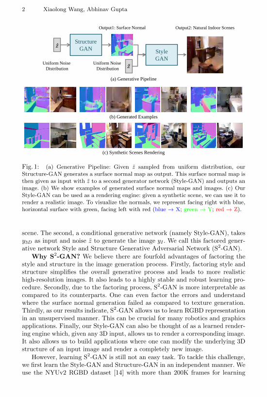
Fig. 1: (a) Generative Pipeline: Given z sampled from uniform distribution, ourStructure-GAN generates a surface normal map as output. This surface normal map isthen given as input with z to a second generator network (Style-GAN) and outputs animage. (b) We show examples of generated surface normal maps and images. (c) OurStyle-GAN can be used as a rendering engine: given a synthetic scene, we can use it torender a realistic image. To visualize the normals, we represent facing right with blue,horizontal surface with green, facing left with red (blue → X; green → Y; red → Z).
scene. The second, a conditional generative network (namely Style-GAN), takesy3D as input and noise z to generate the image yI . We call this factored gener-ative network Style and Structure Generative Adversarial Network (S2-GAN).
Why S2-GAN? We believe there are fourfold advantages of factoring thestyle and structure in the image generation process. Firstly, factoring style andstructure simplifies the overall generative process and leads to more realistichigh-resolution images. It also leads to a highly stable and robust learning pro-cedure. Secondly, due to the factoring process, S2-GAN is more interpretable ascompared to its counterparts. One can even factor the errors and understandwhere the surface normal generation failed as compared to texture generation.Thirdly, as our results indicate, S2-GAN allows us to learn RGBD representationin an unsupervised manner. This can be crucial for many robotics and graphicsapplications. Finally, our Style-GAN can also be thought of as a learned render-ing engine which, given any 3D input, allows us to render a corresponding image.It also allows us to build applications where one can modify the underlying 3Dstructure of an input image and render a completely new image.
However, learning S2-GAN is still not an easy task. To tackle this challenge,we first learn the Style-GAN and Structure-GAN in an independent manner. Weuse the NYUv2 RGBD dataset [14] with more than 200K frames for learning
Generative Image Modeling using Style and Structure Adversarial Networks 3
the initial networks. We train a Structure-GAN using the ground truth surfacenormals from Kinect. Because the perspective distortion of texture is more di-rectly related to normals than to depth, we use surface normal to represent imagestructure in this paper. We learn in parallel our Style-GAN which is conditionalon the ground truth surface normals. While training the Style-GAN, we have twoloss functions: the first loss function takes in an image and the surface normalsand tries to predict if they correspond to a real scene or not. However, this lossfunction alone does not enforce explicit pixel based constraints for aligning gen-erated images with input surface normals. To enforce the pixel-wise constraints,we make the following assumption: if the generated image is realistic enough, weshould be able to reconstruct or predict the 3D structure based on it. We achievethis by adding another discriminator network. More specifically, the generatedimage is not only forwarded to the discriminator network in GAN but also ainput for the trained surface normal predictor network. Once we have trainedan initial Style-GAN and Structure-GAN, we combine them together and per-form end-to-end learning jointly where images are generated from z, z and fedto discriminators for real/fake task.
2 Related Work
Unsupervised learning of visual representation is one of the most challengingproblems in computer vision. There are two primary approaches to unsupervisedlearning. The first is the discriminative approach where we use auxiliary taskssuch that ground truth can be generated without labeling. Some examples ofthese auxiliary tasks include predicting: the relative location of two patches [2],ego-motion in videos [15,16], physical signals [17,18,19].
A more common approach to unsupervised learning is to use a generativeframework. Two types of generative frameworks have been used in the past.Non-parametric approaches perform matching of an image or patch with thedatabase for tasks such as texture synthesis [20] or super-resolution [21]. In thispaper, we are interested in developing a parametric model of images. One com-mon approach is to learn a low-dimensional representation which can be usedto reconstruct an image. Some examples include the deep auto-encoder [22,23]or Restricted Boltzmann machines (RBMs) [24,25,26,27,28]. However, in mostof the above scenarios it is hard to generate new images since sampling in la-tent space is not an easy task. The recently proposed Variational auto-encoders(VAE) [10,11] tackles this problem by generating images with variational sam-pling approach. However, these approaches are restricted to simple datasets suchas MNIST. To generate interpretable images with richer information, the VAEis extended to be conditioned on captions [29] and graphics code [30]. BesidesRBMs and auto-encoders, there are also many novel generative models in re-cent literature [31,32,33,34]. For example, Dosovitskiy et al. [31] proposed to useCNNs to generate chairs.
In this work, we build our model based on the Generative Adversarial Net-works (GANs) framework proposed by Goodfellow et al. [9]. This framework

4 Xiaolong Wang, Abhinav Gupta
was extended by Denton et al. [35] to generate images. Specifically, they pro-posed to use a Laplacian pyramid of adversarial networks to generate images in acoarse to fine scheme. However, training these networks is still tricky and unsta-ble. Therefore, an extension DCGAN [13] proposed good practices for trainingadversarial networks and demonstrated promising results in generating images.There are more extensions include using conditional variables [36,37,38]. For in-stance, Mathieu et al. [37] introduced to predict future video frames conditionedon the previous frames. In this paper, we further simplify the image generationprocess by factoring out the generation of 3D structure and style.
In order to train our S2-GAN we combine adversarial loss with 3D surfacenormal prediction loss [39,40,41,42] to provide extra constraints during learning.This is also related to the idea of combining multiple losses for better generativemodeling [43,44,45]. For example, Makhzani et al. [43] proposed an adversarialauto-encoder which takes the adversarial loss as an extra constraint for the latentcode during training the auto-encoder. Finally, the idea of factorizing image intotwo separate phenomena has been well studied in [46,47,48,49], which motivatesus to decompose the generative process to structure and style. We use the RGBDdata from NYUv2 to factorize and learn a S2-GAN model.
3 Background for Generative Adversarial Networks
The Generative Adversarial Networks (GAN) [9] contains two models: generatorG and discriminator D. The generatorG takes the input which is a latent randomvector z sampled from uniform noise distribution and tries to generate a realisticimage. The discriminator D performs binary classification to distinguish whetheran image is generated from G or it is a real image. Thus the two models arecompeting against each other (hence, adversarial): network G will try to generateimages which will be hard for D to differentiate from real image, meanwhilenetwork D will learn to avoid getting fooled by G.
Formally, we optimize the networks using gradient descent with batch size M .We are given samples as X = (X1, ..., XM ) and a set of z sampled from uniformdistribution as Z = (z1, ..., zM ). The training of GAN is an iterative procedurewith 2 steps: (i) fix the parameters of network G and optimize network D; (ii)fix network D and optimize network G. The loss for training network D is,
LD(X,Z) =
M/2∑i=1
L(D(Xi), 1) +
M∑i=M/2+1
L(D(G(zi)), 0). (1)
Inside a batch, half of images are real and the rest G(zi) are images generated byG given zi. D(Xi) ∈ [0, 1] represents the binary classification score given inputimage Xi. L(y∗, y) = −[y log(y∗) + (1− y)log(1− y∗)] is the binary entropy loss.Thus the loss Eq. 1 for network D is optimized to classify the real image as label1 and the generated image as 0. On the other hand, the generator G is trying tofool D to classify the generated image as a real image via minimizing the loss:
LG(Z) =
M∑i=M/2+1
L(D(G(zi)), 1). (2)
Generative Image Modeling using Style and Structure Adversarial Networks 5
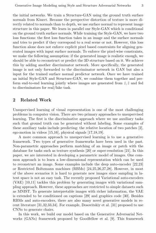
Structure-GAN(G) fc uconv conv conv conv conv uconv conv uconv convInput Size − 9 18 18 18 18 18 36 36 72Kernel Number 9× 9× 64 128 128 256 512 512 256 128 64 3Kernel Size − 4 3 3 3 3 4 3 4 5Stride − 2(up) 1 1 1 1 2(up) 1 2(up) 1
Structure-GAN(D) conv conv conv conv conv fcInput Size 72 36 36 18 9 −Kernel Number 64 128 256 512 128 1Kernel Size 5 5 3 3 3 −Stride 2 1 2 2 1 −
Style-GAN(D) conv conv conv conv conv fcInput Size 128 64 32 16 8 −Kernel Number 64 128 256 512 128 1Kernel Size 5 5 3 3 3 −Stride 2 2 2 2 1 −
Table 1: Network architectures. Top: generator of Structure-GAN; bottom: discrimi-nator of Structure-GAN (left) and discriminator of Style-GAN (right). “conv” meansconvolutional layer, “uconv” means fractionally-strided convolutional (deconvolutional)layer, where 2(up) stride indicates 2x resolution. “fc” means fully connected layer.
4 Style and Structure GAN
GAN and DCGAN approaches directly generate images from the sampled z.Instead, we use the fact that image generation has two components: (a) gener-ating the underlying structure based on the objects in the scene; (b) generatingthe texture/style on top of this 3D structure. We use this simple observationto decompose the generative process into two procedures: (i) Structure-GAN -this process generates surface normals from sampled z and (ii) Style-GAN - thismodel generates the images taking as input the surface normals and anotherlatent variable z sampled from uniform distribution. We train both models withRGBD data, and the ground truth surface normals are obtained from the depth.
4.1 Structure-GAN
We can directly apply GAN framework to learn how to generate surface normalmaps. The input to the network G will be z sampled from uniform distributionand the output is a surface normal map. We use a 100-d vector to represent thez and the output is in size of 72×72×3 (Fig. 2). The discriminator D will learnto classify the generated surface normal maps from the real maps obtained fromdepth. We introduce our network architecture as following.
Generator network. As Table 1 (top row) illustrates, we apply a 10-layermodel for the generator. Given a 100-d z as input, it is first fully connected to a3D block (9×9×64). Then we further perform convolutional operations on top ofit and generate the surface normal map in the end. Note that “uconv” representsfractionally-strided convolution [13], which is also called as deconvolution. Wefollow the settings in [13] and use Batch Normalization [50] and ReLU activationsafter each layer except for the last layer, where a TanH activation is applied.
Discriminator network. We show the 6-layer network architecture in Ta-ble 1 (bottom left). Taking an image as input, the network outputs a singlenumber which predicts the input surface normal is real or generated. We useLeakyReLU [51,52] for activation functions as in [13]. However, we do not apply
6 Xiaolong Wang, Abhinav Gupta
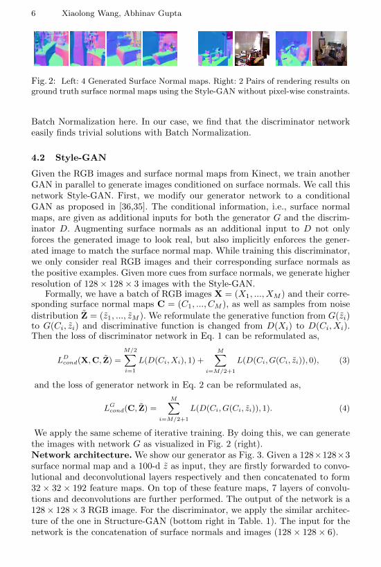
Fig. 2: Left: 4 Generated Surface Normal maps. Right: 2 Pairs of rendering results onground truth surface normal maps using the Style-GAN without pixel-wise constraints.
Batch Normalization here. In our case, we find that the discriminator networkeasily finds trivial solutions with Batch Normalization.
4.2 Style-GAN
Given the RGB images and surface normal maps from Kinect, we train anotherGAN in parallel to generate images conditioned on surface normals. We call thisnetwork Style-GAN. First, we modify our generator network to a conditionalGAN as proposed in [36,35]. The conditional information, i.e., surface normalmaps, are given as additional inputs for both the generator G and the discrim-inator D. Augmenting surface normals as an additional input to D not onlyforces the generated image to look real, but also implicitly enforces the gener-ated image to match the surface normal map. While training this discriminator,we only consider real RGB images and their corresponding surface normals asthe positive examples. Given more cues from surface normals, we generate higherresolution of 128× 128× 3 images with the Style-GAN.
Formally, we have a batch of RGB images X = (X1, ..., XM ) and their corre-sponding surface normal maps C = (C1, ..., CM ), as well as samples from noise
distribution Z = (z1, ..., zM ). We reformulate the generative function from G(zi)to G(Ci, zi) and discriminative function is changed from D(Xi) to D(Ci, Xi).Then the loss of discriminator network in Eq. 1 can be reformulated as,
LDcond(X,C, Z) =
M/2∑i=1
L(D(Ci, Xi), 1) +
M∑i=M/2+1
L(D(Ci, G(Ci, zi)), 0), (3)
and the loss of generator network in Eq. 2 can be reformulated as,
LGcond(C, Z) =
M∑i=M/2+1
L(D(Ci, G(Ci, zi)), 1). (4)
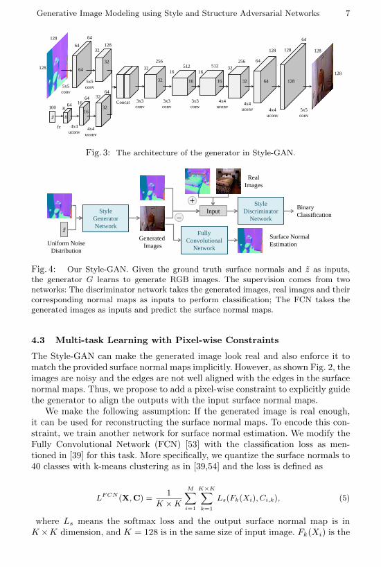
We apply the same scheme of iterative training. By doing this, we can generatethe images with network G as visualized in Fig. 2 (right).Network architecture. We show our generator as Fig. 3. Given a 128×128×3surface normal map and a 100-d z as input, they are firstly forwarded to convo-lutional and deconvolutional layers respectively and then concatenated to form32 × 32 × 192 feature maps. On top of these feature maps, 7 layers of convolu-tions and deconvolutions are further performed. The output of the network is a128× 128× 3 RGB image. For the discriminator, we apply the similar architec-ture of the one in Structure-GAN (bottom right in Table. 1). The input for thenetwork is the concatenation of surface normals and images (128× 128× 6).
Generative Image Modeling using Style and Structure Adversarial Networks 7
64
64
64 32
32
128
128
128
64 8
8
64 16
16 32
32
256
5x5 conv
64 5x5 conv
4x4 uconv
4x4 uconv
3x3 conv
3x3 conv
3x3 conv
4x4 uconv
4x4 uconv 4x4
uconv 5x5 conv
32
32
16
16
512 512
16
16
256 32
32
128
64
64
64
128
128 128
128
Concat
��
100
fc
Fig. 3: The architecture of the generator in Style-GAN.
Style Generator Network
Fully Convolutional
Network
Style Discriminator
Network
Binary Classification Input
−
Surface Normal Estimation
Generated Images
Real Images
��
Uniform Noise Distribution
+
Fig. 4: Our Style-GAN. Given the ground truth surface normals and z as inputs,the generator G learns to generate RGB images. The supervision comes from twonetworks: The discriminator network takes the generated images, real images and theircorresponding normal maps as inputs to perform classification; The FCN takes thegenerated images as inputs and predict the surface normal maps.
4.3 Multi-task Learning with Pixel-wise Constraints
The Style-GAN can make the generated image look real and also enforce it tomatch the provided surface normal maps implicitly. However, as shown Fig. 2, theimages are noisy and the edges are not well aligned with the edges in the surfacenormal maps. Thus, we propose to add a pixel-wise constraint to explicitly guidethe generator to align the outputs with the input surface normal maps.
We make the following assumption: If the generated image is real enough,it can be used for reconstructing the surface normal maps. To encode this con-straint, we train another network for surface normal estimation. We modify theFully Convolutional Network (FCN) [53] with the classification loss as men-tioned in [39] for this task. More specifically, we quantize the surface normals to40 classes with k-means clustering as in [39,54] and the loss is defined as
LFCN (X,C) =1
K ×K
M∑i=1
K×K∑k=1
Ls(Fk(Xi), Ci,k), (5)
where Ls means the softmax loss and the output surface normal map is inK×K dimension, and K = 128 is in the same size of input image. Fk(Xi) is the
8 Xiaolong Wang, Abhinav Gupta
Style Generator Network
Style Discriminator
Network
Generated Images ��
Structure Generator Network
��
Structure Discriminator
Network
Uniform Noise Distribution
Uniform Noise Distribution
Generated Normals
Generated Normals
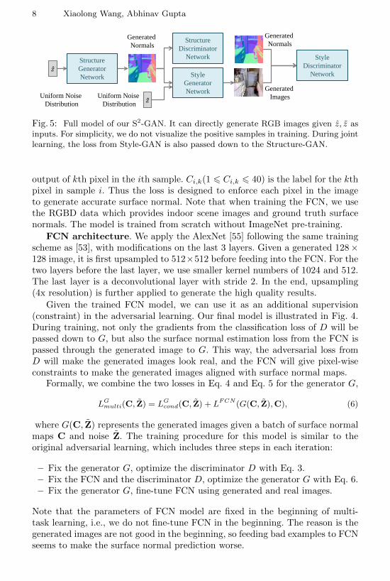
Fig. 5: Full model of our S2-GAN. It can directly generate RGB images given z, z asinputs. For simplicity, we do not visualize the positive samples in training. During jointlearning, the loss from Style-GAN is also passed down to the Structure-GAN.
output of kth pixel in the ith sample. Ci,k(1 6 Ci,k 6 40) is the label for the kthpixel in sample i. Thus the loss is designed to enforce each pixel in the imageto generate accurate surface normal. Note that when training the FCN, we usethe RGBD data which provides indoor scene images and ground truth surfacenormals. The model is trained from scratch without ImageNet pre-training.
FCN architecture. We apply the AlexNet [55] following the same trainingscheme as [53], with modifications on the last 3 layers. Given a generated 128×128 image, it is first upsampled to 512×512 before feeding into the FCN. For thetwo layers before the last layer, we use smaller kernel numbers of 1024 and 512.The last layer is a deconvolutional layer with stride 2. In the end, upsampling(4x resolution) is further applied to generate the high quality results.
Given the trained FCN model, we can use it as an additional supervision(constraint) in the adversarial learning. Our final model is illustrated in Fig. 4.During training, not only the gradients from the classification loss of D will bepassed down to G, but also the surface normal estimation loss from the FCN ispassed through the generated image to G. This way, the adversarial loss fromD will make the generated images look real, and the FCN will give pixel-wiseconstraints to make the generated images aligned with surface normal maps.
Formally, we combine the two losses in Eq. 4 and Eq. 5 for the generator G,
LGmulti(C, Z) = LG
cond(C, Z) + LFCN (G(C, Z),C), (6)
where G(C, Z) represents the generated images given a batch of surface normalmaps C and noise Z. The training procedure for this model is similar to theoriginal adversarial learning, which includes three steps in each iteration:
– Fix the generator G, optimize the discriminator D with Eq. 3.– Fix the FCN and the discriminator D, optimize the generator G with Eq. 6.– Fix the generator G, fine-tune FCN using generated and real images.
Note that the parameters of FCN model are fixed in the beginning of multi-task learning, i.e., we do not fine-tune FCN in the beginning. The reason is thegenerated images are not good in the beginning, so feeding bad examples to FCNseems to make the surface normal prediction worse.
Generative Image Modeling using Style and Structure Adversarial Networks 9
4.4 Joint Learning for S2-GAN
After training the Structure-GAN and Style-GAN independently, we merge allnetworks and train them jointly. As Fig. 5 shows, our full model includes surfacenormal generation from Structure-GAN, and based on it the Style-GAN gener-ates the image. Note that the generated normal maps are first passed throughan upsampling layer with bilinear interpolation before they are forwarded to theStyle-GAN. Since we do not use ground truth surface normal maps to generatethe images, we remove the FCN constraint from the Style-GAN. The discrim-inator in Style-GAN takes generated normals and images as negative samples,and ground truth normals and real images as positive samples.
For the Structure-GAN, the generator network receives not only the gradientsfrom the discriminator of Structure-GAN, but also the gradients passed throughthe generator of Style-GAN. In this way, the network is forced to generate surfacenormals which not only are realistic but also help generate better RGB images.Formally, the loss for the generator network of Structure-GAN can be representedas combining Eq. 2 and Eq. 4,
LGjoint(Z, Z) = LG(Z) + λ · LG
cond(G(Z), Z) (7)
where Z = (z1, ..., zM ) and Z = (z1, ..., zM ) represent two sets of samplesdrawn from uniform distribution for Structure-GAN and Style-GAN respectively.The first term in Eq. 7 represents the adversarial loss from the discriminator ofStructure-GAN and the second term represents that the loss of the Style-GANis also passed down. We set the coefficient λ = 0.1 and smaller learning rate forStructure-GAN than Style-GAN in the experiments, so that we can prevent thegenerated normals from over fitting to the task of generating RGB images viaStyle-GAN. In our experiments, we find that without constraining λ and learningrates, the loss LG(Z) easily diverges to high values and the Structure-GAN canno longer generate reasonable surface normal maps.
5 Experiments
We perform two types of experiments: (a) We qualitatively and quantitativelyevaluate the quality of images generates using our model; (b) We evaluate thequality of unsupervised representation learning by applying the network for dif-ferent tasks such as image classification and object detection.Dataset. We use the NYUv2 dataset [14] in our experiment. We use the rawvideo data during training and extract 200K frames from the 249 training videoscenes. We compute the surface normals from the depth as [42,39].Parameter Settings. We follow the parameters in [13] for training. We trainedthe models using Adam optimizer [56] with momentum term β1 = 0.5, β2 = 0.999and batch size M = 128. The inputs and outputs for all networks are scaled to[−1, 1] (including surface normals and RGB images). During training the Styleand Structure GANs separately, we set the learning rate to 0.0002. We train theStructure-GAN for 25 epochs. For Style-GAN, we first fix the FCN model andtrain it for 25 epochs, then the FCN model are fine-tuned together with 5 more
10 Xiaolong Wang, Abhinav Gupta
Input Output Original Input Output Original Input Output Original
Input Output Input Output Input Output Input Output
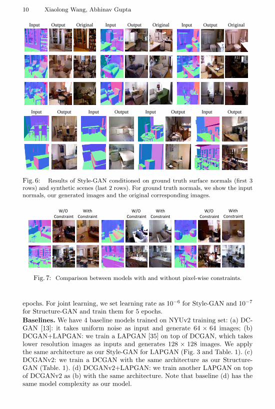
Fig. 6: Results of Style-GAN conditioned on ground truth surface normals (first 3rows) and synthetic scenes (last 2 rows). For ground truth normals, we show the inputnormals, our generated images and the original corresponding images.
W/O Constraint
With Constraint
W/O Constraint
With Constraint
W/O Constraint
With Constraint
Fig. 7: Comparison between models with and without pixel-wise constraints.
epochs. For joint learning, we set learning rate as 10−6 for Style-GAN and 10−7
for Structure-GAN and train them for 5 epochs.
Baselines. We have 4 baseline models trained on NYUv2 training set: (a) DC-GAN [13]: it takes uniform noise as input and generate 64 × 64 images; (b)DCGAN+LAPGAN: we train a LAPGAN [35] on top of DCGAN, which takeslower resolution images as inputs and generates 128 × 128 images. We applythe same architecture as our Style-GAN for LAPGAN (Fig. 3 and Table. 1). (c)DCGANv2: we train a DCGAN with the same architecture as our Structure-GAN (Table. 1). (d) DCGANv2+LAPGAN: we train another LAPGAN on topof DCGANv2 as (b) with the same architecture. Note that baseline (d) has thesame model complexity as our model.
Generative Image Modeling using Style and Structure Adversarial Networks 11
(a) Indoor scenes generated by our method
(b) Indoor scenes generated by DCGAN
(c) Indoor scenes generated by DCGAN + LAPGAN
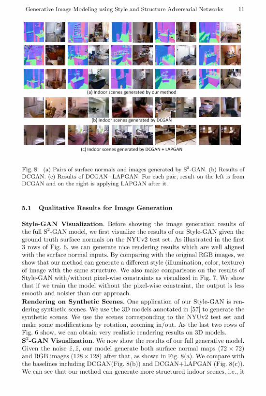
Fig. 8: (a) Pairs of surface normals and images generated by S2-GAN. (b) Results ofDCGAN. (c) Results of DCGAN+LAPGAN. For each pair, result on the left is fromDCGAN and on the right is applying LAPGAN after it.
5.1 Qualitative Results for Image Generation
Style-GAN Visualization. Before showing the image generation results ofthe full S2-GAN model, we first visualize the results of our Style-GAN given theground truth surface normals on the NYUv2 test set. As illustrated in the first3 rows of Fig. 6, we can generate nice rendering results which are well alignedwith the surface normal inputs. By comparing with the original RGB images, weshow that our method can generate a different style (illumination, color, texture)of image with the same structure. We also make comparisons on the results ofStyle-GAN with/without pixel-wise constraints as visualized in Fig. 7. We showthat if we train the model without the pixel-wise constraint, the output is lesssmooth and noisier than our approach.
Rendering on Synthetic Scenes. One application of our Style-GAN is ren-dering synthetic scenes. We use the 3D models annotated in [57] to generate thesynthetic scenes. We use the scenes corresponding to the NYUv2 test set andmake some modifications by rotation, zooming in/out. As the last two rows ofFig. 6 show, we can obtain very realistic rendering results on 3D models.
S2-GAN Visualization. We now show the results of our full generative model.Given the noise z, z, our model generate both surface normal maps (72 × 72)and RGB images (128×128) after that, as shown in Fig. 8(a). We compare withthe baselines including DCGAN(Fig. 8(b)) and DCGAN+LAPGAN (Fig. 8(c)).We can see that our method can generate more structured indoor scenes, i.e., it
12 Xiaolong Wang, Abhinav Gupta
Fix Structure &
Change Style
Fix Structure &
Change Style
Fix Style &
Change Structure
Fix Style &
Change Structure
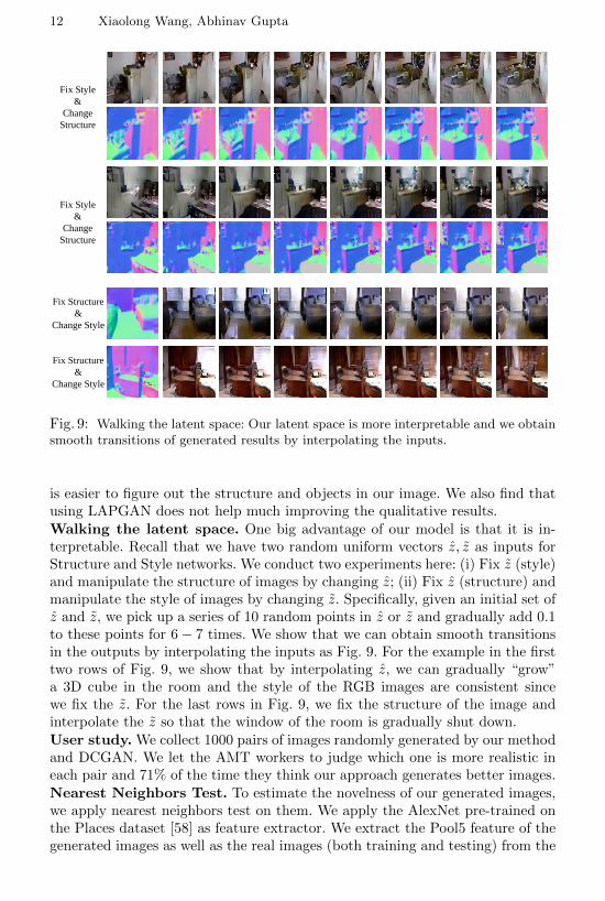
Fig. 9: Walking the latent space: Our latent space is more interpretable and we obtainsmooth transitions of generated results by interpolating the inputs.
is easier to figure out the structure and objects in our image. We also find thatusing LAPGAN does not help much improving the qualitative results.Walking the latent space. One big advantage of our model is that it is in-terpretable. Recall that we have two random uniform vectors z, z as inputs forStructure and Style networks. We conduct two experiments here: (i) Fix z (style)and manipulate the structure of images by changing z; (ii) Fix z (structure) andmanipulate the style of images by changing z. Specifically, given an initial set ofz and z, we pick up a series of 10 random points in z or z and gradually add 0.1to these points for 6− 7 times. We show that we can obtain smooth transitionsin the outputs by interpolating the inputs as Fig. 9. For the example in the firsttwo rows of Fig. 9, we show that by interpolating z, we can gradually “grow”a 3D cube in the room and the style of the RGB images are consistent sincewe fix the z. For the last rows in Fig. 9, we fix the structure of the image andinterpolate the z so that the window of the room is gradually shut down.User study. We collect 1000 pairs of images randomly generated by our methodand DCGAN. We let the AMT workers to judge which one is more realistic ineach pair and 71% of the time they think our approach generates better images.Nearest Neighbors Test. To estimate the novelness of our generated images,we apply nearest neighbors test on them. We apply the AlexNet pre-trained onthe Places dataset [58] as feature extractor. We extract the Pool5 feature of thegenerated images as well as the real images (both training and testing) from the
Generative Image Modeling using Style and Structure Adversarial Networks 13
Query Nearest Neighbors Results
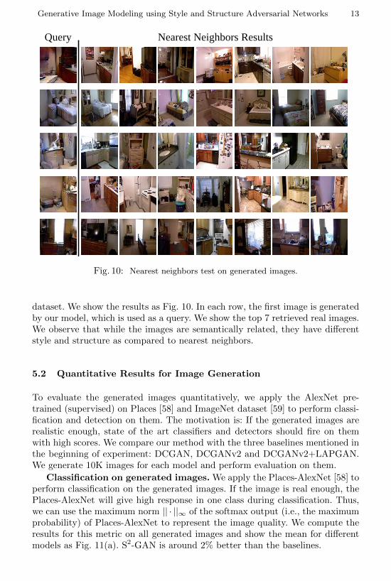
Fig. 10: Nearest neighbors test on generated images.
dataset. We show the results as Fig. 10. In each row, the first image is generatedby our model, which is used as a query. We show the top 7 retrieved real images.We observe that while the images are semantically related, they have differentstyle and structure as compared to nearest neighbors.
5.2 Quantitative Results for Image Generation
To evaluate the generated images quantitatively, we apply the AlexNet pre-trained (supervised) on Places [58] and ImageNet dataset [59] to perform classi-fication and detection on them. The motivation is: If the generated images arerealistic enough, state of the art classifiers and detectors should fire on themwith high scores. We compare our method with the three baselines mentioned inthe beginning of experiment: DCGAN, DCGANv2 and DCGANv2+LAPGAN.We generate 10K images for each model and perform evaluation on them.
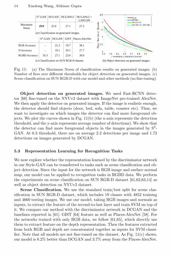
Classification on generated images. We apply the Places-AlexNet [58] toperform classification on the generated images. If the image is real enough, thePlaces-AlexNet will give high response in one class during classification. Thus,we can use the maximum norm || · ||∞ of the softmax output (i.e., the maximumprobability) of Places-AlexNet to represent the image quality. We compute theresults for this metric on all generated images and show the mean for differentmodels as Fig. 11(a). S2-GAN is around 2% better than the baselines.
14 Xiaolong Wang, Abhinav Gupta
(a) Classification on generated images.
(b) Object detection on generated images.
S2-GAN
Maximum Norm
DCGAN DCGANv2 DCGANv2 + LAPGAN
29.0 25.6 27.1 27.2
S2-GAN
RGB Accuracy
DCGAN GIST Places-AlexNet
- 21.3 19.7
D Accuracy
RGBD Accuracy
-
35.3
19.1
27.1
20.1
23.0
38.1
27.7
39.0
(c) Classification on SUN RGB-D dataset.
Fig. 11: (a) The Maximum Norm of classification results on generated images. (b)Number of fires over different thresholds for object detection on generated images. (c)Scene classification on SUN RGB-D with our model and other methods (no fine-tuning).
Object detection on generated images. We used Fast-RCNN detec-tor [60] fine-tuned on the NYUv2 dataset with ImageNet pre-trained AlexNet.We then apply the detector on generated images. If the image is realistic enough,the detector should find objects (door, bed, sofa, table, counter etc). Thus, wewant to investigate on which images the detector can find more foreground ob-jects. We plot the curves shown in Fig. 11(b) (the x-axis represents the detectionthreshold, and the y-axis represents average number of detections). We show thatthe detector can find more foreground objects in the images generated by S2-GAN. At 0.3 threshold, there are on average 2.2 detections per image and 1.72detections on images generated by DCGAN.
5.3 Representation Learning for Recognition Tasks
We now explore whether the representation learned by the discriminator networkin our Style-GAN can be transferred to tasks such as scene classification and ob-ject detection. Since the input for the network is RGB image and surface normalmap, our model can be applied to recognition tasks in RGBD data. We performthe experiments on scene classification on SUN RGB-D dataset [61,62,63,14] aswell as object detection on NYUv2 dataset.
Scene Classification. We use the standard train/test split for scene clas-sification in SUN RGB-D dataset, which includes 19 classes with 4852 trainingand 4660 testing images. We use our model, taking RGB images and normals asinputs, to extract the feature of the second-to-last layer and train SVM on top ofit. We compare our method with the discriminator network in DCGAN and thebaselines reported in [61]: GIST [64] feature as well as Places-AlexNet [58]. Forthe networks trained with only RGB data, we follow [61,65], which directly usethem to extract feature on the depth representation. Then the features extractedfrom both RGB and depth are concatenated together as inputs for SVM classi-fier. Note that all models are not fine-tuned on the dataset. As Fig. 11(c) shows,our model is 8.2% better than DCGAN and 3.7% away from the Places-AlexNet.
Generative Image Modeling using Style and Structure Adversarial Networks 15
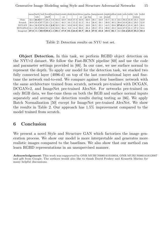
mean bath bed book box chair count- desk door dress- garba- lamp monit- night pillow sink sofa table tele toilettub shelf -er -er -ge bin -or stand vision
Ours 32.4 44.0 67.7 28.4 1.6 34.2 43.9 10.0 17.3 33.9 22.6 28.1 24.8 41.7 31.3 33.1 50.2 21.9 25.1 54.9Scratch 30.9 35.6 67.7 23.1 2.1 33.1 40.5 10.1 15.2 31.2 19.4 26.8 29.1 39.9 30.5 36.6 43.8 20.4 29.5 52.8DCGAN 30.4 38.9 67.6 26.3 2.9 32.5 39.1 10.6 16.9 23.6 23.0 26.5 25.1 44.5 29.6 37.0 45.2 21.0 28.5 38.4
DCGANv2 31.1 35.3 69.0 21.5 2.0 32.6 36.4 9.8 14.4 30.8 25.4 29.2 27.3 39.6 32.2 34.6 47.9 21.1 27.2 54.4Imagenet 37.6 33.1 69.9 39.6 2.3 38.1 47.9 16.1 24.6 40.7 26.5 37.8 45.6 49.5 36.1 34.5 53.2 25.0 35.3 58.4
Table 2: Detection results on NYU test set.
Object Detection. In this task, we perform RGBD object detection onthe NYUv2 dataset. We follow the Fast-RCNN pipeline [60] and use the codeand parameter settings provided in [66]. In our case, we use surface normal torepresent the depth. To apply our model for the detection task, we stacked twofully connected layer (4096-d) on top of the last convolutional layer and fine-tune the network end-to-end. We compare against four baselines: network withthe same architecture trained from scratch, network pre-trained with DCGAN,DCGANv2, and ImageNet pre-trained AlexNet. For networks pre-trained ononly RGB data, we fine-tune them on both the RGB and surface normal inputsseparately and average the detection results during testing as [66]. We applyBatch Normalization [50] except for ImageNet pre-trained AlexNet. We showthe results in Table 2. Our approach has 1.5% improvement compared to themodel trained from scratch.
6 Conclusion
We present a novel Style and Structure GAN which factorizes the image gen-eration process. We show our model is more interpretable and generates morerealistic images compared to the baselines. We also show that our method canlearn RGBD representations in an unsupervised manner.
Acknowledgement: This work was supported by ONR MURI N000141010934, ONR MURI N000141612007and gift from Google. The authors would also like to thank David Fouhey and Kenneth Marino formany helpful discussions.
16 Xiaolong Wang, Abhinav Gupta
References
1. Doersch, C., Gupta, A., Efros, A.A.: Context as supervisory signal: Discoveringobjects with predictable context. In: ECCV. (2014)
2. Doersch, C., Gupta, A., Efros, A.A.: Unsupervised visual representation learningby context prediction. In: ICCV. (2015)
3. Wang, X., Gupta, A.: Unsupervised learning of visual representations using videos.In: ICCV. (2015)
4. Goroshin, R., Bruna, J., Tompson, J., Eigen, D., LeCun, Y.: Unsupervised learningof spatiotemporally coherent metrics. ICCV (2015)
5. Zou, W.Y., Zhu, S., Ng, A.Y., Yu, K.: Deep learning of invariant features viasimulated fixations in video. In: NIPS. (2012)
6. Li, Y., Paluri, M., Rehg, J.M., Dollar, P.: Unsupervised learning of edges. In:CVPR. (2016)
7. Walker, J., Gupta, A., Hebert, M.: Dense optical flow prediction from a staticimage. In: ICCV. (2015)
8. Misra, I., Zitnick, C.L., Hebert, M.: Shuffle and learn: Unsupervised learning usingtemporal order verification. In: ECCV. (2016)
9. Goodfellow, I., Pouget-Abadie, J., Mirza, M., Xu, B., Warde-Farley, D., Ozair, S.,Courville, A., Bengio, Y.: Generative adversarial nets. In: NIPS. (2014)
10. Kingma, D., Welling, M.: Auto-encoding variational bayes. In: ICLR. (2014)11. Gregor, K., Danihelka, I., Graves, A., Rezende, D.J., Wierstra, D.: Draw: A recur-
rent neural network for image generation. CoRR abs/1502.04623 (2015)12. Li, Y., Swersky, K., Zemel, R.: Generative moment matching networks. In: ICML.
(2014)13. Radford, A., Metz, L., Chintala, S.: Unsupervised representation learning with
deep convolutional generative adversarial networks. CoRR abs/1511.06434(2015)
14. Silberman, N., Hoiem, D., Kohli, P., Fergus, R.: Indoor segmentation and supportinference from RGBD images. In: ECCV. (2012)
15. Agrawal, P., Carreira, J., Malik, J.: Learning to see by moving. In: ICCV. (2015)16. Jayaraman, D., Grauman, K.: Learning image representations tied to ego-motion.
In: ICCV. (2015)17. Owens, A., Isola, P., McDermott, J., Torralba, A., Adelson, E., Freeman, W.:
Visually indicated sounds. In: CVPR. (2016)18. Pinto, L., Gupta, A.: Supersizing self-supervision: Learning to grasp from 50k tries
and 700 robot hours. In: ICRA. (2016)19. Pinto, L., Gandhi, D., Han, Y., Park, Y.L., Gupta, A.: The curious robot: Learning
visual representations via physical interactions. In: ECCV. (2016)20. Efros, A.A., Leung, T.K.: Texture synthesis by non-parametric sampling. In:
ICCV. (1999)21. Freeman, W.T., Jones, T.R., Pasztor, E.C.: Example-based super-resolution. In:
Computer Graphics and Applications. (2002)22. Bengio, Y., Lamblin, P., Popovici, D., Larochelle, H.: Greedy layer-wise training
of deep networks. In: NIPS. (2007)23. Le, Q.V., Ranzato, M.A., Monga, R., Devin, M., Chen, K., Corrado, G.S., Dean,
J., Ng, A.Y.: Building high-level features using large scale unsupervised learning.In: ICML. (2012)
24. Ranzato, M.A., Krizhevsky, A., Hinton, G.E.: Factored 3-way restricted boltzmannmachines for modeling natural images. In: AISTATS. (2010)
Generative Image Modeling using Style and Structure Adversarial Networks 17
25. Osindero, S., Hinton, G.E.: Modeling image patches with a directed hierarchy ofmarkov random fields. In: NIPS. (2008)
26. Hinton, G.E., Salakhutdinov, R.R.: Reducing the dimensionality of data withneural networks. Science 313 (2006) 504–507
27. Lee, H., Grosse, R., Ranganath, R., Ng, A.Y.: Convolutional deep belief networksfor scalable unsupervised learning of hierarchical representations. In: ICML. (2009)
28. Taylor, G.W., Hinton, G.E., Roweis, S.: Modeling human motion using binarylatent variables. In: NIPS. (2006)
29. Mansimov, E., Parisotto, E., Ba, J.L., Salakhutdinov, R.: Generating images fromcaptions with attention. CoRR abs/1511.02793 (2015)
30. Kulkarni, T.D., Whitney, W.F., Kohli, P., Tenenbaum, J.B.: Deep convolutionalinverse graphics network. In: NIPS. (2015)
31. Dosovitskiy, A., Springenberg, J.T., Brox, T.: Learning to generate chairs withconvolutional neural networks. In: CVPR. (2015)
32. Tatarchenko, M., Dosovitskiy, A., Brox, T.: Single-view to multi-view: Recon-structing unseen views with a convolutional network. CoRR abs/1511.06702(2015)
33. Theis, L., Bethge, M.: Generative image modeling using spatial lstms. CoRRabs/1506.03478 (2015)
34. Oord, A.V.D., Kalchbrenner, N., Kavukcuoglu, K.: Pixel recurrent neural networks.CoRR abs/1601.06759 (2016)
35. Denton, E., Chintala, S., Szlam, A., Fergus, R.: Deep generative image modelsusing a laplacian pyramid of adversarial networks. In: NIPS. (2015)
36. Mirza, M., Osindero, S.: Conditional generative adversarial nets. CoRRabs/1411.1784 (2014)
37. Mathieu, M., Couprie, C., LeCun, Y.: Deep multi-scale video prediction beyondmean square error. CoRR abs/1511.05440 (2015)
38. Im, D.J., Kim, C.D., Jiang, H., Memisevic, R.: Generating images with recurrentadversarial networks. CoRR abs/1602.05110 (2016)
39. Wang, X., Fouhey, D.F., Gupta, A.: Designing deep networks for surface normalestimation. In: CVPR. (2015)
40. Eigen, D., Fergus, R.: Predicting depth, surface normals and semantic labels witha common multi-scale convolutional architecture. In: ICCV. (2015)
41. Fouhey, D.F., Gupta, A., Hebert, M.: Data-driven 3D primitives for single imageunderstanding. In: ICCV. (2013)
42. Ladicky, L., Zeisl, B., Pollefeys, M.: Discriminatively trained dense surface normalestimation. In: ECCV. (2014)
43. Makhzani, A., Shlens, J., Jaitly, N., Goodfellow, I.J.: Adversarial autoencoders.CoRR abs/1511.05644 (2015)
44. Larsen, A.B.L., Sønderby, S.K., Winther, O.: Autoencoding beyond pixels using alearned similarity metric. CoRR abs/1512.09300 (2015)
45. Dosovitskiy, A., Brox, T.: Generating images with perceptual similarity metricsbased on deep networks. CoRR abs/1602.02644 (2016)
46. Barrow, H.G., Tenenbaum, J.M.: Recovering intrinsic scene characteristics fromimages. In: Computer Vision Systems. (1978)
47. Tenenbaum, J.B., Freeman, W.T.: Separating style and content with bilinear mod-els. In: Neural Computation. (2000)
48. Fouhey, D.F., Hussain, W., Gupta, A., Hebert, M.: Single image 3d without asingle 3d image. In: ICCV. (2015)
49. Zhu, S.C., Wu, Y.N., Mumford, D.: Filters, random fields and maximum entropy(frame): Towards a unified theory for texture modeling. In: IJCV. (1998)
18 Xiaolong Wang, Abhinav Gupta
50. Ioffe, S., Szegedy, C.: Batch normalization: Accelerating deep network training byreducing internal covariate shift. CoRR abs/1502.03167 (2015)
51. Maas, A.L., Hannun, A.Y., Ng, A.Y.: Rectifier nonlinearities improve neural net-work acoustic models. In: ICML. (2013)
52. Xu, B., Wang, N., Chen, T., Li, M.: Empirical evaluation of rectified activationsin convolutional network. CoRR abs/1505.00853 (2015)
53. Long, J., Shelhamer, E., Darrell, T.: Fully convolutional networks for semanticsegmentation. In: CVPR. (2015)
54. Ladicky, L., Shi, J., Pollefeys, M.: Pulling things out of perspective. In: cvpr.(2014)
55. Krizhevsky, A., Sutskever, I., Hinton, G.E.: Imagenet classification with deepconvolutional neural networks. In: NIPS. (2012)
56. Kingma, D., Ba, J.: Adam: A method for stochastic optimization. CoRRabs/1412.6980 (2014)
57. Guo, R., Hoiem, D.: Support surface prediction in indoor scenes. In: ICCV. (2013)58. Zhou, B., Lapedriza, A., Xiao, J., Torralba, A., Oliva, A.: Learning deep features
for scene recognition using places database. In: NIPS. (2014)59. Russakovsky, O., Deng, J., Su, H., Krause, J., Satheesh, S., Ma, S., Huang, Z.,
Karpathy, A., Khosla, A., Bernstein, M., Berg, A.C., Fei-Fei, L.: ImageNet LargeScale Visual Recognition Challenge. IJCV 115(3) (2015) 211–252
60. Girshick, R.: Fast r-cnn. In: ICCV. (2015)61. Song, S., Lichtenberg, S., Xiao, J.: Sun rgb-d: A rgb-d scene understanding bench-
mark suite. In: CVPR. (2015)62. Janoch, A., Karayev, S., Jia, Y., Barron, J., Fritz, M., Saenko, K., Darrell, T.: A
category-level 3-d object dataset: Putting the kinect to work. In: Workshop onConsumer Depth Cameras in Computer Vision (with ICCV). (2011)
63. Xiao, J., Owens, A., Torralba, A.: Sun3d: A database of big spaces reconstructedusing sfm and object labels. In: ICCV. (2013)
64. Oliva, A., Torralba, A.: Modeling the shape of the scene: A holistic representationof the spatial envelope. IJCV (2011)
65. Gupta, S., Girshick, R., Arbelez, P., Malik, J.: Learning rich features from rgb-dimages for object detection and segmentation. In: ECCV. (2014)
66. Gupta, S., Hoffman, J., Malik, J.: Cross modal distillation for supervision transfer.In: CVPR. (2016)
Generative Image Modeling using Style and Structure Adversarial Networks 19
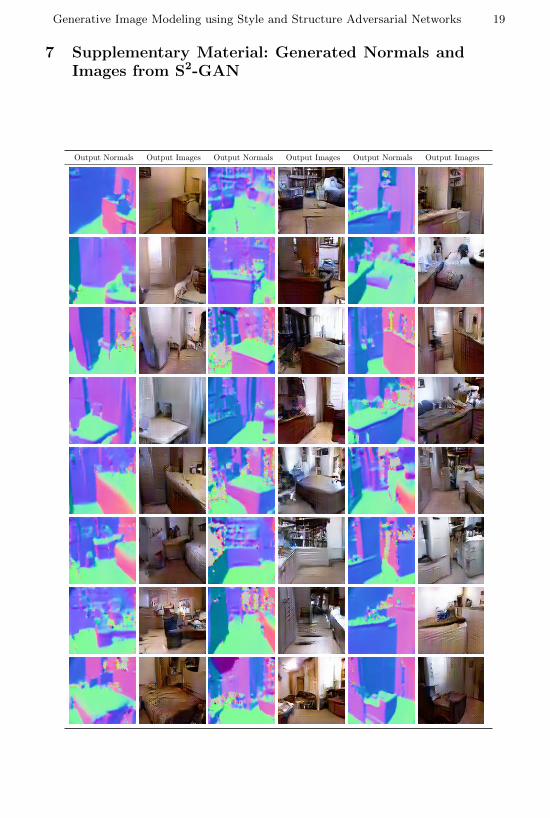
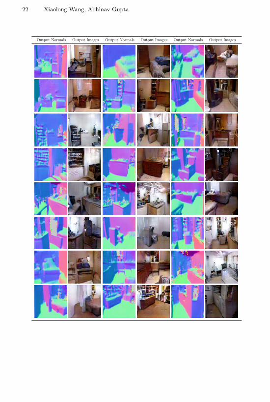
7 Supplementary Material: Generated Normals andImages from S2-GAN
Output Normals Output Images Output Normals Output Images Output Normals Output Images
20 Xiaolong Wang, Abhinav Gupta
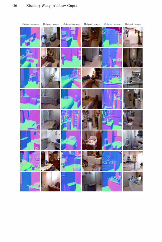
Output Normals Output Images Output Normals Output Images Output Normals Output Images
Generative Image Modeling using Style and Structure Adversarial Networks 21
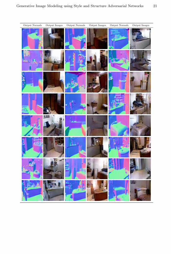
Output Normals Output Images Output Normals Output Images Output Normals Output Images
22 Xiaolong Wang, Abhinav Gupta
Output Normals Output Images Output Normals Output Images Output Normals Output Images