Embed Size (px)
Citation preview

Genetic ConservationGenetic ConservationGenetic ConservationGenetic Conservation ofofofof EEEEndangered ndangered ndangered ndangered AAAAnimal nimal nimal nimal PPPPopulationsopulationsopulationsopulations
Promotor: Prof. dr. ir. Johan A.M. van Arendonk Hoogleraar in de Fokkerij en Genetica Wageningen Universiteit Co-promotor: Dr. ir. Piter Bijma Universitair Docent, leerstoelgroep Fokkerij en Genetica Wageningen Universiteit Promotiecommissie: Prof. John A.Woolliams Roslin Institute, Edinburgh, United Kingdom Prof. Dr. Henner Simianer Universität Göttingen, Germany Prof. dr. Rolf F. Hoekstra Wageningen Universiteit Dr. ir. J.K.(Kor) Oldenbroek Wageningen Universiteit
Dit proefschrift is uitgevoerd binnen de onderzoekschool WIAS
Genetic Genetic Genetic Genetic ConservationConservationConservationConservation ofofofof EEEEndangered ndangered ndangered ndangered AAAAnimal nimal nimal nimal PPPPopulationsopulationsopulationsopulations
Pieter A. OliehoekPieter A. OliehoekPieter A. OliehoekPieter A. Oliehoek Proefschrift ter verkrijging van de graad van doctor op gezag van de rector magnificus van Wageningen Universiteit, Prof.dr. M.J. Kropff, in het openbaar te verdedigen op dinsdag 14 april 2009 des middags te half twee in de Aula.
Genetic Conservation of Genetic Conservation of Genetic Conservation of Genetic Conservation of EEEEndangered ndangered ndangered ndangered AAAAnimal nimal nimal nimal PPPPopulationsopulationsopulationsopulations
Pieter Oliehoek, 2009 ISBN: 978ISBN: 978ISBN: 978ISBN: 978----90909090----8585858585858585----350350350350----3333
PhD thesis, Wageningen University
Table of ContentsTable of ContentsTable of ContentsTable of Contents
Chapter 1 General Introduction 1 Chapter 2 Cluster analysis of kinship reveals structure 11
of the closed pedigreed population of the Icelandic Sheepdog
Chapter 3 Effects of pedigree errors 27
on the efficiency of conservation decisions Chapter 4 Correction of kinship for unknown parents 41 with a focus on their use in conservation programs Chapter 5 Estimating relatedness between individuals 57
in general populations with a focus on their use in conservation programs
Chapter 6 General Discussion 83 Literature Cited 100 Summary 104 Samenvatting 108 Curriculum Vitae 111

------------------------------------------------------------------------------------------------------------------------------------------------------------------------------------------------------------------------------------------------------------------------------------------------------------------------------------------------------------------------------------------------------------------------------------------------------------------------------------------------------------------------------------------------------------------------------------------------------------------------------------------------ ------------------------------------------------------------------------------------------------------------------------------------------------------------------------------------------------------------------------------------------------------------------------------------------------------------------------------------------------------------------------------------------------------------------------------------------------------------------------------------------------------------------------------------------------------------------------------------------------------------------------
1
"The world is changing. I can feel it in the water I can feel it in the earth I can smell it in the air Much that once was is lost For none now live who remember it.”
J R R Tolkien - Lord of the Rings
General IntroductionGeneral IntroductionGeneral IntroductionGeneral Introduction
C h a p t e r 1C h a p t e r 1C h a p t e r 1C h a p t e r 1
LLLLOSS OF OSS OF OSS OF OSS OF BBBBIODIVERSITYIODIVERSITYIODIVERSITYIODIVERSITY DIAMOND (2005) stated in “Collapse” that destruction of ecosystems was one of
the major causes of collapses of most human civilizations that happened in history. These collapses were preceded by human population growth. Human (population) expansion itself also led to extinction of animal species throughout history DIAMOND (1997). For example, with most new settlements of human on uninhabited continents or island, the megafauna disappeared. Human expansion and extinction of species is now happening on global scale. SMIL (2002) quantified the result of human expansion in megaton of carbon. In 2000, biomass of 6 billion people was roughly 40 megatons of carbon. Domestic animals had then a biomass of roughly 100 megatons of carbon. The biomass of all wild vertebrates on land was roughly only 5 megatons. Human activities are now responsible for over 95% of biomass occupied by vertebrates on land. While in 1804 the world counted one billion people, today (November 2008) the world counts over 6.7 billion people. With such an increase within two centuries, further extinction of species is expected. Indeed a massive extinction of life started during the last century with about one species every 20 minutes (WILSON, 1992). At this rate, one fifth of all
-------------------- G e n e r a l I n t r o d u c t i o n G e n e r a l I n t r o d u c t i o n G e n e r a l I n t r o d u c t i o n G e n e r a l I n t r o d u c t i o n ------------------------------------------------------------------------------------------------------------------------------------------------------------------------------------------------------------------------------------------------------------------------------------------------------------------------------------------------------------------------------------------------------------------------------------------------------------------------------------------------------------------------------------------------------------------------------------------------------------------------------------------------------------------------------------------------------------------------------------------------------------------------------------------------------------------------------------------------------------------------------------
-------------------------------------------------------------------------------------------------------------------------------------------------------------------------------------------------------------------------------------------------------------------------------------------------------------------------------------------------------------------------------------------------------------------------------------------------------------------------------------------------------------------------------------------------------------------------------------------------------------------------------------------- ----------------------------------------------------------------------------------------------------------------------------------------------------------------------------------------------------------------------------------------------------------------------------------------------------------------------------------------------------------------------------------------------------------------------------------------------------------------------------------------------------------------------------------------------------------------------------------------------------------------
2
species will be extinct before 2031 (WILSON, 2002). Of four mammal species, two decline in population size and one is threatened with extinction, with loss of habitat as primary cause (SCHIPPER et al., 2008).
On the other hand the Convention on Biological Diversity in Rio de Janeiro in 1992 recognized for the first time in international law that the conservation of biological diversity is "a common concern of humankind". The agreement covers all ecosystems, species, and genetic resources. New agreements commit countries to conserve biodiversity, develop resources for sustainability, and share the benefits resulting from their use.
In conclusion, due to human activities, many wild animal (sub-)species decreased in population size, became fragmented, are (critically) endangered. Only deliberate actions can avoid further extinction. For some species, the only option is ex situ conservation, either captive breeding and/or cryo-conservation. If current rate of human populations growth continues (and there is no reason to assume it will not), more species will rely on ex situ conservation for survival. Within this scenario, two major concerns arise: (1) populations that are fragmented or have a small population size will lose genetic diversity; and (2) captive breeding is costly. Hence, managing genetic diversity within captive populations is a necessity for (a) getting populations out of a bottleneck and (b) efficient breeding strategies for conservation.
Though the number of domestic animals has increased tremendously, this does not necessarily favor genetic diversity for domestic species. Despite their growth in numbers, the last two centuries were also characterized by a decline of genetic diversity within domestic species as well. Three factors are involved: (1) introduction of breed-studbooks, which led to exclusion of domestic animals that did not belong to ‘a breed’; (2) preferential breeding of few specific high performance breeds; (3) preferential breeding with specific individuals, especially males within breeds. At least one domestic animal breed has become extinct each month over the past seven years, and around 20% of the breeds of the primary domestic animal species (cattle, goats, pigs, horses and poultry) are at risk of extinction (RISCHKOWSKY and PILLING, 2007).
Genetic diversity is critical for conservation of endangered populations. Genetic diversity is correlated with adaptive capacity of populations. Reduction of genetic diversity is eventually followed by higher levels of inbreeding, which can cause inbreeding depression as well as high incidence of particular heritable recessive diseases. Small populations are at risk of decreasing or even losing genetic diversity due to unavoidable low number of available parents (candidates). However, also larger populations might lose genetic diversity, caused by the low number of candidates selected.
------------------------------------------------------------------------------------------------------------------------------------------------------------------------------------------------------------------------------------------------------------------------------------------------------------------------------------------------------------------------------------------------------------------------------------------------------------------------------------------------------------------------------------------------------------------------------------------------------------------------------------------------------------------------------------------------------------------------------------------------------------------------------------------------------------------------------------------------------------------------------------------------------------------------------------------------------------------------------------------------------------------------------------------------------------------------------------------------ C h a p t e r 1C h a p t e r 1C h a p t e r 1C h a p t e r 1 --------------------
------------------------------------------------------------------------------------------------------------------------------------------------------------------------------------------------------------------------------------------------------------------------------------------------------------------------------------------------------------------------------------------------------------------------------------------------------------------------------------------------------------------------------------------------------------------------------------------------------------------------------------------------ ------------------------------------------------------------------------------------------------------------------------------------------------------------------------------------------------------------------------------------------------------------------------------------------------------------------------------------------------------------------------------------------------------------------------------------------------------------------------------------------------------------------------------------------------------------------------------------------------------------------------
3
GGGGENETIC ENETIC ENETIC ENETIC MMMMANAGEMENT OF ANAGEMENT OF ANAGEMENT OF ANAGEMENT OF SSSSMALL MALL MALL MALL AAAANIMAL NIMAL NIMAL NIMAL PPPPOPULATIONSOPULATIONSOPULATIONSOPULATIONS The previous paragraph explains the need for management of genetic diversity
within small animal populations for both wild and domestic species. This thesis investigated methods to support conservation of genetic diversity within populations. The research focused on minimizing kinship as a conservation method; and the efficiency of minimizing kinship when observed kinship (what breeders think they have) deviates from the true kinship. This chapter describes the concept of kinship; conservation strategies that minimize kinship; the diversity measures that are used throughout this thesis; and finally an outline of the thesis.
KKKKINSHIP WINSHIP WINSHIP WINSHIP WITHIN ITHIN ITHIN ITHIN PPPPOPULATIONSOPULATIONSOPULATIONSOPULATIONS Kinship (or coancestry) of two animals is the probability that two alleles sampled
randomly, one from each animal, are ‘identical by descent’ (IBD), indicating that they descend from a common ancestor (FALCONER and MACKAY, 1996). Estimation or calculation of kinship needs data as starting point (LYNCH and WALSH, 1997), either pedigrees or a set of molecular markers. Hence, data like known pedigrees and/or molecular markers for each animal in the population forms the basis for estimating kinship. The quality of the data will determine accuracy of kinship.
Kinship is expressed relative to a so-called base population (FALCONER and MACKAY, 1996). In the base population, all alleles are defined as being not-IBD, so that kinship among individuals and inbreeding in the base population is zero by definition. The choice of the base population is arbitrary. However, not all choices are genetically meaningful and theoretically correct, particularly in structured populations (see also Chapter 2 and 5).
Kinship and pedigrees:Kinship and pedigrees:Kinship and pedigrees:Kinship and pedigrees: In the case of pedigree, the base population is determined by its founders. Founders are defined as animals that are unrelated to each other. They do not share alleles IBD by definition. All other animals of a population descend from founder animals. Note that founders do not necessarily have to live in the same period. All subsequent calculations of kinship trace common ancestries only as far back as this founder stock. Except for mutations, no closed population can have more genetic diversity than did the founders (LACY, 1995). Within this thesis, mutation is ignored, since populations with low number of animals will have a very low chance to gain genetic diversity due to mutations. The common way to calculate kinship from (complex) pedigree is the tabular method (EMIK and TERRILL, 1949) which starts with the founders and calculates kinship for every individual with every other individual down to the current population.
-------------------- G e n e r a l I n t r o d u c t i o n G e n e r a l I n t r o d u c t i o n G e n e r a l I n t r o d u c t i o n G e n e r a l I n t r o d u c t i o n ------------------------------------------------------------------------------------------------------------------------------------------------------------------------------------------------------------------------------------------------------------------------------------------------------------------------------------------------------------------------------------------------------------------------------------------------------------------------------------------------------------------------------------------------------------------------------------------------------------------------------------------------------------------------------------------------------------------------------------------------------------------------------------------------------------------------------------------------------------------------------------
-------------------------------------------------------------------------------------------------------------------------------------------------------------------------------------------------------------------------------------------------------------------------------------------------------------------------------------------------------------------------------------------------------------------------------------------------------------------------------------------------------------------------------------------------------------------------------------------------------------------------------------------- ----------------------------------------------------------------------------------------------------------------------------------------------------------------------------------------------------------------------------------------------------------------------------------------------------------------------------------------------------------------------------------------------------------------------------------------------------------------------------------------------------------------------------------------------------------------------------------------------------------------
4
Kinship and molecular markers:Kinship and molecular markers:Kinship and molecular markers:Kinship and molecular markers: Besides pedigree, also molecular markers can be used to estimate kinship by relatedness estimators (alias kinship estimators). Several relatedness estimators have been proposed in literature, which are compared in Chapter 5. As explained previously, kinship should be based on alleles ‘identical by descent’ (IBD). When two individuals share similar alleles, they might not be identical due to common ancestry, but due to chance. Those alleles are biochemically ‘alike in state’ (AIS). Thus, to determine kinship, it is needed to determine the probability of alleles being AIS. In the base population, animals by definition do not share common ancestors. Alleles that are identical in the base population are, therefore all due to AIS. Intuitively, it is logical that, for example, a base population with 100 founders will not have 200 unique alleles on each locus. Some alleles will be similar simply due to chance (AIS). Theoretically, those alleles will be spread equally among animals of the base population (founders).
Relatedness estimators differ in the way they determine probability of alleles AIS (and implicitly the base population). This is further explained in Chapter 5.
CCCCONSERVATION ONSERVATION ONSERVATION ONSERVATION SSSSTRATEGIESTRATEGIESTRATEGIESTRATEGIES Genetic diversity can be maximized by giving higher contributions to genetically
important animals (BALLOU and LACY, 1995). In this paragraph, we describe three conservation strategies that aim to maximize genetic diversity.
Equalizing founder contributions: Equalizing founder contributions: Equalizing founder contributions: Equalizing founder contributions: Equalizing founder contributions implicitly attempts to equalize allele frequencies (and thus minimize kinship). Genetically important animals are those animals that descend from unique founders. In practice, however, equalizing founder contributions is often impossible due to mixing of unique founder alleles with overrepresented alleles (BALLOU and LACY, 1995). Furthermore, equalizing founder contributions is an inefficient strategy, because contributions from all ancestors should be managed, not only from founders (WOOLLIAMS, 2007).
Mean Kinship:Mean Kinship:Mean Kinship:Mean Kinship: BALLOU and LACY (1995) proposed mean kinship as a conservation strategy and concluded from model simulations that mean kinship performed significantly better than random breeding and equalizing founder contributions, for all pedigrees provided. Breeding with animals having low ‘mean kinship’ is regarded as good practice within conservation genetics (BALLOU and LACY, 1995; FRANKHAM et al., 2002) and is applied in many zoo populations. Mean kinship of individual i (mki) is defined as the average of the kinship coefficients between that individual and all other candidates (currently living and fertile animals) including itself:
∑=
=�
j
iji�
mk1
ƒ1
,, ((11))
where N is the number of candidates in the population and ƒij is the kinship between individual i an individual j. Individuals with low mean kinship represent
------------------------------------------------------------------------------------------------------------------------------------------------------------------------------------------------------------------------------------------------------------------------------------------------------------------------------------------------------------------------------------------------------------------------------------------------------------------------------------------------------------------------------------------------------------------------------------------------------------------------------------------------------------------------------------------------------------------------------------------------------------------------------------------------------------------------------------------------------------------------------------------------------------------------------------------------------------------------------------------------------------------------------------------------------------------------------------------------ C h a p t e r 1C h a p t e r 1C h a p t e r 1C h a p t e r 1 --------------------
------------------------------------------------------------------------------------------------------------------------------------------------------------------------------------------------------------------------------------------------------------------------------------------------------------------------------------------------------------------------------------------------------------------------------------------------------------------------------------------------------------------------------------------------------------------------------------------------------------------------------------------------ ------------------------------------------------------------------------------------------------------------------------------------------------------------------------------------------------------------------------------------------------------------------------------------------------------------------------------------------------------------------------------------------------------------------------------------------------------------------------------------------------------------------------------------------------------------------------------------------------------------------------
5
important animals. Note that mean kinship depends on the population. Hence, mean kinship of a specific animal might change over time when a population changes, for example mean kinship will increase each time an animal produces progeny. The goal of using animals having low mean kinship, is to lower the average mean kinship (mk ) of the population. mk is calculated by the average of mean kinships of all animals within the population under study (BALLOU and LACY, 1995). Thus, mk can be calculated as follows:
∑∑= =
=�
i
�
j
ijf�
mk1 1
2
1,, ((22))
Optimal Contribution Selection (OCS): Optimal Contribution Selection (OCS): Optimal Contribution Selection (OCS): Optimal Contribution Selection (OCS): OCS is a strategy that is able to calculate contributions per candidates (fertile animals) so that the weighted average mean kinship among candidates is minimized. Optimal contributions are obtained in the following way. Average mean kinship among candidates is given by MEUWISSEN (1997):
ECECmk Fc'c= ((33))
where FFFF is a matrix of kinships between all candidates, including kinship of candidates with themselves and ccccEC is a column vector of equal contributions for each candidate to the next generation, so that the sum of elements of ccccEC equals one. Note that Equation 2 and 3 would produce the same result. Average mean kinship among candidates, and thus the mk level in future generations, can be decreased or increased by varying the contributions of candidates (cccc). Thus average mean kinship can be minimized by finding an optimum contribution vector ccccOC that minimizes cccc’’’’FcFcFcFc, which is given by MEUWISSEN (1997) and EDING et al. (2002):
1F1'
1Fc
1
1
−
−
=OC,, ((44))
where 1111 is a column vector of one’s. Theoretically, OCS could minimize average mean kinship by selection of only
few candidates. In practice, it has been observed that the introduction of a single animal can lead to an increase of genetic variance (INGVARSSON, 2002), indicating that a high contribution of specific animals can indeed increase genetic diversity. Optimal contributions are sensitive. Small differences in pedigree might be the difference between a significant and zero contribution assigned to a candidate. For example, when both parents are still fertile, contribution of the offspring will be zero. As soon as one parent is no longer available (dead or infertile), the contribution of its offspring will increase.
In theory, OCS is the most efficient method to minimize kinship (SONESSON and MEUWISSEN, 2001; PONG-WONG and WOOLLIAMS, 2007). Within animal breeding OCS is a mature selection method that can consider both genetic gain (improvement of performance of animals) as well as maintaining genetic diversity (WOOLLIAMS, 2006).
-------------------- G e n e r a l I n t r o d u c t i o n G e n e r a l I n t r o d u c t i o n G e n e r a l I n t r o d u c t i o n G e n e r a l I n t r o d u c t i o n ------------------------------------------------------------------------------------------------------------------------------------------------------------------------------------------------------------------------------------------------------------------------------------------------------------------------------------------------------------------------------------------------------------------------------------------------------------------------------------------------------------------------------------------------------------------------------------------------------------------------------------------------------------------------------------------------------------------------------------------------------------------------------------------------------------------------------------------------------------------------------------
-------------------------------------------------------------------------------------------------------------------------------------------------------------------------------------------------------------------------------------------------------------------------------------------------------------------------------------------------------------------------------------------------------------------------------------------------------------------------------------------------------------------------------------------------------------------------------------------------------------------------------------------- ----------------------------------------------------------------------------------------------------------------------------------------------------------------------------------------------------------------------------------------------------------------------------------------------------------------------------------------------------------------------------------------------------------------------------------------------------------------------------------------------------------------------------------------------------------------------------------------------------------------
6
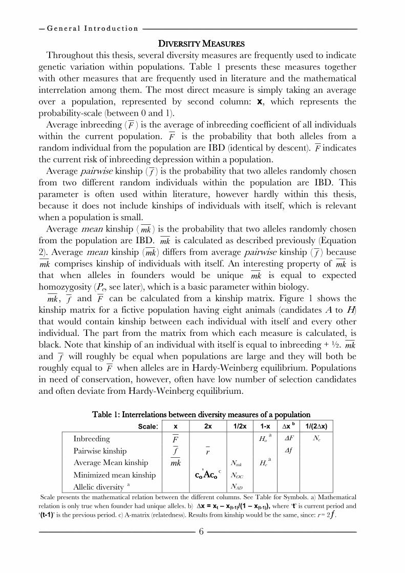
DDDDIVERSITY IVERSITY IVERSITY IVERSITY MMMMEASURESEASURESEASURESEASURES Throughout this thesis, several diversity measures are frequently used to indicate
genetic variation within populations. Table 1 presents these measures together with other measures that are frequently used in literature and the mathematical interrelation among them. The most direct measure is simply taking an average over a population, represented by second column: x, which represents the probability-scale (between 0 and 1).
Average inbreeding (F ) is the average of inbreeding coefficient of all individuals within the current population. F is the probability that both alleles from a random individual from the population are IBD (identical by descent). F indicates the current risk of inbreeding depression within a population.
Average pairwise kinship ( f ) is the probability that two alleles randomly chosen from two different random individuals within the population are IBD. This parameter is often used within literature, however hardly within this thesis, because it does not include kinships of individuals with itself, which is relevant when a population is small.
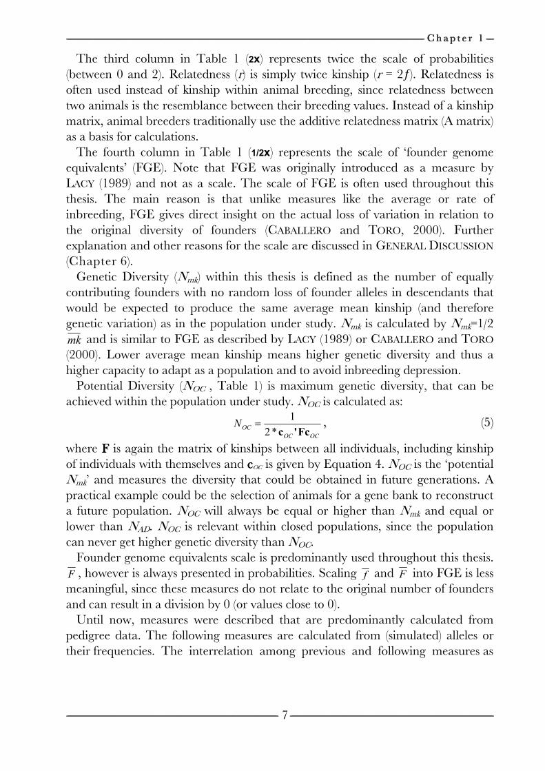
Average mean kinship ( ) is the probability that two alleles randomly chosen from the population are IBD. is calculated as described previously (Equation 2). Average mean kinship (mk ) differs from average pairwise kinship ( f ) because mk comprises kinship of individuals with itself. An interesting property of mk is that when alleles in founders would be unique mk is equal to expected homozygosity (Pe, see later), which is a basic parameter within biology. mk , f and F can be calculated from a kinship matrix. Figure 1 shows the
kinship matrix for a fictive population having eight animals (candidates A to H) that would contain kinship between each individual with itself and every other individual. The part from the matrix from which each measure is calculated, is black. Note that kinship of an individual with itself is equal to inbreeding + ½. mk and f will roughly be equal when populations are large and they will both be roughly equal to F when alleles are in Hardy-Weinberg equilibrium. Populations in need of conservation, however, often have low number of selection candidates and often deviate from Hardy-Weinberg equilibrium.
Table 1: Interrelations between diversity measures of a populationTable 1: Interrelations between diversity measures of a populationTable 1: Interrelations between diversity measures of a populationTable 1: Interrelations between diversity measures of a population
Scale: x 2x 1/2x 1-x ∆x b
1/(2∆x)
Inbreeding F Ho a
∆F Ne
Pairwise kinship f r ∆ƒ
Average Mean kinship mk
Nmk. He a
Minimized mean kinship ccccoooo’’’’AcAcAcAcoooo
c NOC
Allelic diversity a NAD
Scale presents the mathematical relation between the different columns. See Table for Symbols. a) Mathematical relation is only true when founder had unique alleles. b) ∆x = xt – x(t-1)/(1 – x(t-1)), where ‘t’ is current period and ‘(t-1)’ is the previous period. c) A-matrix (relatedness). Results from kinship would be the same, since: r = 2ƒ.
mk
mk
------------------------------------------------------------------------------------------------------------------------------------------------------------------------------------------------------------------------------------------------------------------------------------------------------------------------------------------------------------------------------------------------------------------------------------------------------------------------------------------------------------------------------------------------------------------------------------------------------------------------------------------------------------------------------------------------------------------------------------------------------------------------------------------------------------------------------------------------------------------------------------------------------------------------------------------------------------------------------------------------------------------------------------------------------------------------------------------------ C h a p t e r 1C h a p t e r 1C h a p t e r 1C h a p t e r 1 --------------------
------------------------------------------------------------------------------------------------------------------------------------------------------------------------------------------------------------------------------------------------------------------------------------------------------------------------------------------------------------------------------------------------------------------------------------------------------------------------------------------------------------------------------------------------------------------------------------------------------------------------------------------------ ------------------------------------------------------------------------------------------------------------------------------------------------------------------------------------------------------------------------------------------------------------------------------------------------------------------------------------------------------------------------------------------------------------------------------------------------------------------------------------------------------------------------------------------------------------------------------------------------------------------------
7
The third column in Table 1 (2x) represents twice the scale of probabilities (between 0 and 2). Relatedness (r) is simply twice kinship (r = 2ƒ). Relatedness is often used instead of kinship within animal breeding, since relatedness between two animals is the resemblance between their breeding values. Instead of a kinship matrix, animal breeders traditionally use the additive relatedness matrix (A matrix) as a basis for calculations.
The fourth column in Table 1 (1/2x) represents the scale of ‘founder genome equivalents’ (FGE). Note that FGE was originally introduced as a measure by LACY (1989) and not as a scale. The scale of FGE is often used throughout this thesis. The main reason is that unlike measures like the average or rate of inbreeding, FGE gives direct insight on the actual loss of variation in relation to the original diversity of founders (CABALLERO and TORO, 2000). Further explanation and other reasons for the scale are discussed in GENERAL DISCUSSION (Chapter 6).
Genetic Diversity (Nmk) within this thesis is defined as the number of equally contributing founders with no random loss of founder alleles in descendants that would be expected to produce the same average mean kinship (and therefore genetic variation) as in the population under study. Nmk is calculated by Nmk=1/2mk and is similar to FGE as described by LACY (1989) or CABALLERO and TORO
(2000). Lower average mean kinship means higher genetic diversity and thus a higher capacity to adapt as a population and to avoid inbreeding depression.
Potential Diversity (NOC , Table 1) is maximum genetic diversity, that can be achieved within the population under study. NOC is calculated as:
OCOC
OC�Fc'c*2
1= ,, ((55))
where FFFF is again the matrix of kinships between all individuals, including kinship of individuals with themselves and ccccOC is given by Equation 4. NOC is the ‘potential Nmk’ and measures the diversity that could be obtained in future generations. A practical example could be the selection of animals for a gene bank to reconstruct a future population. NOC will always be equal or higher than Nmk and equal or lower than NAD. NOC is relevant within closed populations, since the population can never get higher genetic diversity than NOC.
Founder genome equivalents scale is predominantly used throughout this thesis. F , however is always presented in probabilities. Scaling f and F into FGE is less meaningful, since these measures do not relate to the original number of founders and can result in a division by 0 (or values close to 0).
Until now, measures were described that are predominantly calculated from pedigree data. The following measures are calculated from (simulated) alleles or their frequencies. The interrelation among previous and following measures as
-------------------- G e n e r a l I n t r o d u c t i o n G e n e r a l I n t r o d u c t i o n G e n e r a l I n t r o d u c t i o n G e n e r a l I n t r o d u c t i o n ------------------------------------------------------------------------------------------------------------------------------------------------------------------------------------------------------------------------------------------------------------------------------------------------------------------------------------------------------------------------------------------------------------------------------------------------------------------------------------------------------------------------------------------------------------------------------------------------------------------------------------------------------------------------------------------------------------------------------------------------------------------------------------------------------------------------------------------------------------------------------------
-------------------------------------------------------------------------------------------------------------------------------------------------------------------------------------------------------------------------------------------------------------------------------------------------------------------------------------------------------------------------------------------------------------------------------------------------------------------------------------------------------------------------------------------------------------------------------------------------------------------------------------------- ----------------------------------------------------------------------------------------------------------------------------------------------------------------------------------------------------------------------------------------------------------------------------------------------------------------------------------------------------------------------------------------------------------------------------------------------------------------------------------------------------------------------------------------------------------------------------------------------------------------
8
Figure 1: Calculation of average inbreeding and kinshFigure 1: Calculation of average inbreeding and kinshFigure 1: Calculation of average inbreeding and kinshFigure 1: Calculation of average inbreeding and kinship from kinship matrixip from kinship matrixip from kinship matrixip from kinship matrix
Kinship matrix is based on a population of 8 individuals A until H.
Each square within the matrix contain kinship (ƒij) between individual i and j.
presented in Table 1, are only true when all founder alleles would be unique (AIS and IBD is zero in the base population).
Allelic Diversity (NAD) is half the number of distinct alleles that are still present in the population under study if all founder alleles would be unique. It is the number of founders that would have the same number of unique alleles as the population under study. The total number of distinct alleles in pedigreed populations can be determined by a genedrop from founders (LACY, 1995). NAD is also on the scale of FGE and can therefore be compared with Nmk and NOC.
Table 1, sixth column: 1-x gives measures that are basic parameters in classical genetics. Expected Heterozygosity (He) is one minus Expected Homozygosity (Pe) and is calculated by:
∑=
−=−=A
a
aee pPH1
211 ,, ((66))
where A is the number of distinct alleles and pa is the frequency of allele a. Observed Heterozygosity (Ho) is the observed proportion of heterozygous loci (per individual or all individuals in a population). Expected homozygosity (Pe) serve as starting point for some relatedness estimators (Chapter 5).
OOOOUTLINE OF THIS UTLINE OF THIS UTLINE OF THIS UTLINE OF THIS TTTTHESISHESISHESISHESIS Optimal contribution selection calculated from kinship is the most effective
conservation strategy if one authority has full control over a population and quality of data on kinship between animals (pedigree or molecular markers) is excellent. In practice, quality of data is almost never perfect and this thesis investigates consequences of deviations of the ideal case. It will investigate the influence of data that is not excellent on the possibilities to increase or maintain genetic diversity with optimal contribution selection. Furthermore, this thesis investigates the influence of deviations of the ‘observed’ (estimated) kinship from the true kinship and how to correct for detected deviations.
------------------------------------------------------------------------------------------------------------------------------------------------------------------------------------------------------------------------------------------------------------------------------------------------------------------------------------------------------------------------------------------------------------------------------------------------------------------------------------------------------------------------------------------------------------------------------------------------------------------------------------------------------------------------------------------------------------------------------------------------------------------------------------------------------------------------------------------------------------------------------------------------------------------------------------------------------------------------------------------------------------------------------------------------------------------------------------------------ C h a p t e r 1C h a p t e r 1C h a p t e r 1C h a p t e r 1 --------------------
------------------------------------------------------------------------------------------------------------------------------------------------------------------------------------------------------------------------------------------------------------------------------------------------------------------------------------------------------------------------------------------------------------------------------------------------------------------------------------------------------------------------------------------------------------------------------------------------------------------------------------------------ ------------------------------------------------------------------------------------------------------------------------------------------------------------------------------------------------------------------------------------------------------------------------------------------------------------------------------------------------------------------------------------------------------------------------------------------------------------------------------------------------------------------------------------------------------------------------------------------------------------------------
9
ChapterChapterChapterChapter 2222 (CLUSTER ANALYSIS OF KINSHIP REVEALS STRUCTURE OF THE
CLOSED PEDIGREED POPULATION OF THE ICELANDIC SHEEPDOG) compares kinship calculated up to seven generations with kinship calculated including all generations. In the latter, the base generation consist of all true founders (animals that are unrelated to each other; however not necessarily all in the same generation). In the first, the base generation is implicitly defined by the seventh generation. ChapterChapterChapterChapter 2222 uses the Icelandic Sheepdog breed as an example of a closed pedigreed population. The chapter discusses the genetic history of the breed and the possibilities of preservation of genetic diversity considering the multi-breeder aspect of this population.
Pedigrees that serve as data to calculate kinship among animals do not always reflect the actual genealogy. Two chapters deal with this problem. ChapterChapterChapterChapter 3333 (EFFECTS OF ERRORS IN PEDIGREES ON THE EFFICIENCY OF CONSERVATION
DECISIONS) investigates the influence of wrong as well as missing pedigree information on possibilities to apply optimal contribution selection. This chapter makes use of simulation to determine the actual genetic diversity saved by applying optimal contributions based on pedigrees that contain errors. ChapterChapterChapterChapter 4444 (CORRECTION OF KINSHIP FOR UNKNOWN PARENTS IN CONSERVATION
PROGRAMS) investigates different ways to deal with missing pedigree information (gaps in pedigrees), which is traditionally bypassed by assuming that animals without recorded parents are also unrelated to founders. This chapter uses pedigrees from zoo populations having non-founder animals without recorded parents, as a template for simulations. Complete pedigrees were simulated from the pedigree having gaps. Hereafter, different ways to correct for gaps were applied on the original pedigree and compared with the ‘simulated’ complete pedigree.
If pedigrees are insufficient in quality (or not present at all), genetic management can still be applied using molecular markers as data to estimate kinship. ChapterChapterChapterChapter 5555 (ESTIMATING RELATEDNESS BETWEEN INDIVIDUALS IN GENERAL
POPULATIONS WITH A FOCUS ON THEIR USE IN CONSERVATION PROGRAMS) compares different relatedness (2 × kinship) estimators that make use of molecular markers and investigates their ability to preserve genetic diversity. ChapterChapterChapterChapter 5555 also makes use of simulations that produce both panmictic and structured populations having both true pedigree and molecular marker data. Hence, kinship estimated from molecular markers is compared with the true kinship calculated from pedigree.
ChapterChapterChapterChapter 6666 (GENERAL DISCUSSION) discusses the implications of the chapters 2 until 5 on the maintenance of genetic diversity for endangered animal populations.
----------------------------------------------------------------------------------------------------------------------------------------------------------------------------------------------------------------------------------------------------------------------------------------------------------------------------------------------------------------------------------------------------------------------------------------------------------------------------------------------------------------------------------------------------------------------------------------------------------------------------------------------------------------------------------------------------------------------------------------------------------------------------------------------------------------------------------------------------------------------------------------------------------------------------------------------------------------------------------------------------------------------------------------------------------------------------------------------------------------------------------------------------------------------------------------------------------------------------------------------------------------------------------------------------------------
-------------------------------------------------------------------------------------------------------------------------------------------------------------------------------------------------------------------------------------------------------------------------------------------------------------------------------------------------------------------------------------------------------------------------------------------------------------------------------------------------------------------------------------------------------------------------------------------------------------------------------------------- ----------------------------------------------------------------------------------------------------------------------------------------------------------------------------------------------------------------------------------------------------------------------------------------------------------------------------------------------------------------------------------------------------------------------------------------------------------------------------------------------------------------------------------------------------------------------------------------------------------------
10
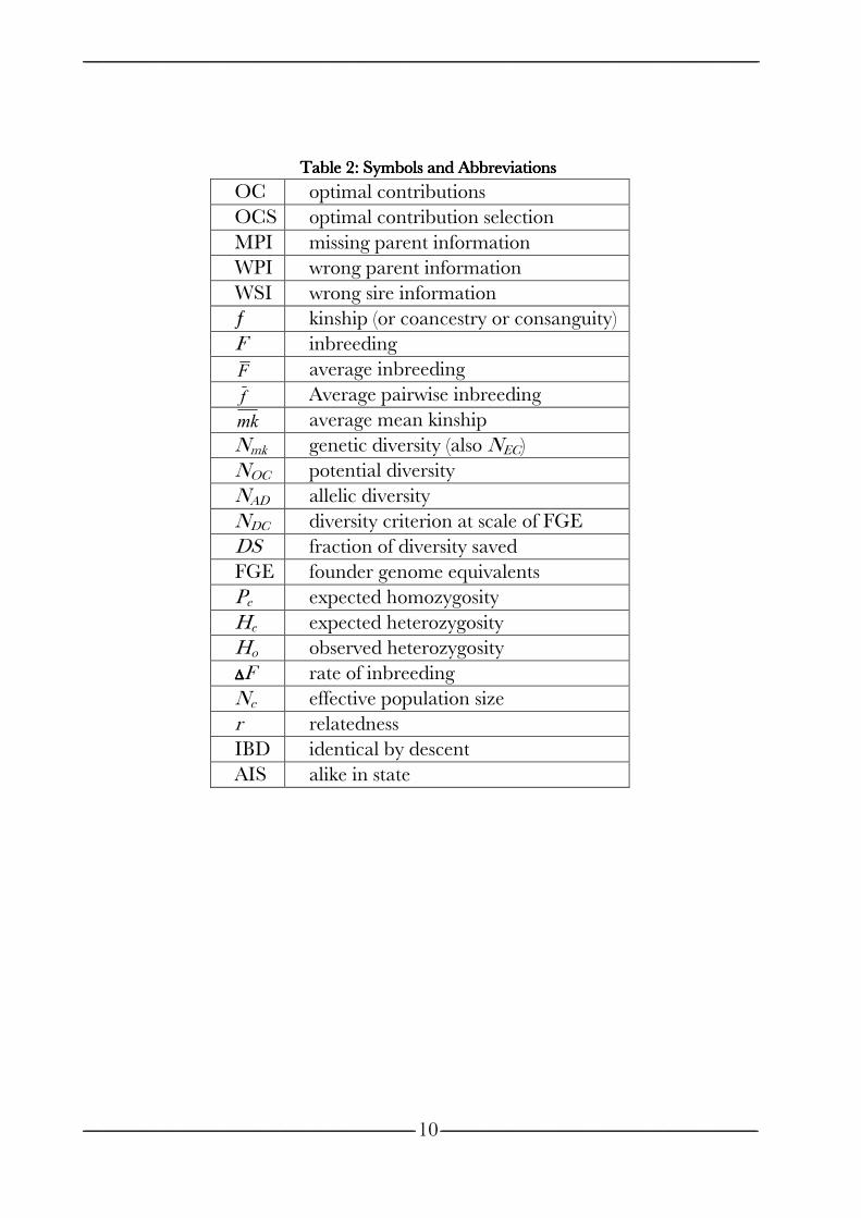
Table 2: Table 2: Table 2: Table 2: Symbols and Symbols and Symbols and Symbols and AbbreviationsAbbreviationsAbbreviationsAbbreviations
OC optimal contributions OCS optimal contribution selection MPI missing parent information WPI wrong parent information WSI wrong sire information ƒ kinship (or coancestry or consanguity) F inbreeding F average inbreeding f Average pairwise inbreeding mk average mean kinship Nmk genetic diversity (also NEC) NOC potential diversity NAD allelic diversity NDC diversity criterion at scale of FGE DS fraction of diversity saved FGE founder genome equivalents Pe expected homozygosity He expected heterozygosity Ho observed heterozygosity ∆∆∆∆F rate of inbreeding Ne effective population size r relatedness IBD identical by descent AIS alike in state
----------------------------------------------------------------------------------------------------------------------------------------------------------------------------------------------------------------------------------------------------------------------------------------------------------------------------------------------------------------------------------------------------------------------------------------------------------------------------------------------------------------------------------------------------------------------------------------------------------------------------------------------------------------------------------------------------------------------------------------------------------------------------------------------------------------------------------------------------------------------------------------------------------------------------------------------------------------------------------------------------------------------------------------------------------------------------------------------------------------------------------------------------------------------------------------------------------------------------------------------------------------------------------------------------------------
-------------------------------------------------------------------------------------------------------------------------------------------------------------------------------------------------------------------------------------------------------------------------------------------------------------------------------------------------------------------------------------------------------------------------------------------------------------------------------------------------------------------------------------------------------------------------------------------------------------------------------------------- ----------------------------------------------------------------------------------------------------------------------------------------------------------------------------------------------------------------------------------------------------------------------------------------------------------------------------------------------------------------------------------------------------------------------------------------------------------------------------------------------------------------------------------------------------------------------------------------------------------------
11
Cluster analysis of kinship reveals structure Cluster analysis of kinship reveals structure Cluster analysis of kinship reveals structure Cluster analysis of kinship reveals structure
of the closed pedigreed population of of the closed pedigreed population of of the closed pedigreed population of of the closed pedigreed population of
the Icelandic Sheepdogthe Icelandic Sheepdogthe Icelandic Sheepdogthe Icelandic Sheepdog
C h a p t e r 2C h a p t e r 2C h a p t e r 2C h a p t e r 2
Pieter A. Oliehoek *, Piter Bijma * and Arie van der Meijden ‡
* Animal Breeding and Genomics Centre, Wageningen University, The Netherlands
‡ Trier Faculty of Geography/Geosciences, Biogeography Department, Trier University, Germany
Submitted to Genetics Selection Evolution
-------------------- C l u s t e r a n a l y s i s r e v e a l s d i v e r s i t y C l u s t e r a n a l y s i s r e v e a l s d i v e r s i t y C l u s t e r a n a l y s i s r e v e a l s d i v e r s i t y C l u s t e r a n a l y s i s r e v e a l s d i v e r s i t y ----------------------------------------------------------------------------------------------------------------------------------------------------------------------------------------------------------------------------------------------------------------------------------------------------------------------------------------------------------------------------------------------------------------------------------------------------------------------------------------------------------------------------------------------------------------------------------------------------------------------------------------------------------------
-------------------------------------------------------------------------------------------------------------------------------------------------------------------------------------------------------------------------------------------------------------------------------------------------------------------------------------------------------------------------------------------------------------------------------------------------------------------------------------------------------------------------------------------------------------------------------------------------------------------------------------------- ----------------------------------------------------------------------------------------------------------------------------------------------------------------------------------------------------------------------------------------------------------------------------------------------------------------------------------------------------------------------------------------------------------------------------------------------------------------------------------------------------------------------------------------------------------------------------------------------------------------
12
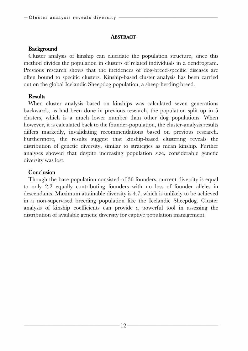
AAAABSTRACTBSTRACTBSTRACTBSTRACT
BackgroundBackgroundBackgroundBackground Cluster analysis of kinship can elucidate the population structure, since this
method divides the population in clusters of related individuals in a dendrogram. Previous research shows that the incidences of dog-breed-specific diseases are often bound to specific clusters. Kinship-based cluster analysis has been carried out on the global Icelandic Sheepdog population, a sheep-herding breed.
ResultsResultsResultsResults When cluster analysis based on kinships was calculated seven generations
backwards, as had been done in previous research, the population split up in 5 clusters, which is a much lower number than other dog populations. When however, it is calculated back to the founder-population, the cluster-analysis results differs markedly, invalidating recommendations based on previous research. Furthermore, the results suggest that kinship-based clustering reveals the distribution of genetic diversity, similar to strategies as mean kinship. Further analyses showed that despite increasing population size, considerable genetic diversity was lost.
ConclusionConclusionConclusionConclusion Though the base population consisted of 36 founders, current diversity is equal
to only 2.2 equally contributing founders with no loss of founder alleles in descendants. Maximum attainable diversity is 4.7, which is unlikely to be achieved in a non-supervised breeding population like the Icelandic Sheepdog. Cluster analysis of kinship coefficients can provide a powerful tool in assessing the distribution of available genetic diversity for captive population management.
------------------------------------------------------------------------------------------------------------------------------------------------------------------------------------------------------------------------------------------------------------------------------------------------------------------------------------------------------------------------------------------------------------------------------------------------------------------------------------------------------------------------------------------------------------------------------------------------------------------------------------------------------------------------------------------------------------------------------------------------------------------------------------------------------------------------------------------------------------------------------------------------------------------------------------------------------------------------------------------------------------------------------------------------------------------------------------------------ C h a p t e r C h a p t e r C h a p t e r C h a p t e r 2222 --------------------
---------------------------------------------------------------------------------------------------------------------------------------------------------------------------------------------------------------------------------------------------------------------------------------------------------------------------------------------------------------------------------------------------------------------------------------------------------------------------------------------------------------------------------------------------------------------------------------------------------------------------------------- --------------------------------------------------------------------------------------------------------------------------------------------------------------------------------------------------------------------------------------------------------------------------------------------------------------------------------------------------------------------------------------------------------------------------------------------------------------------------------------------------------------------------------------------------------------------------------------------------------
13
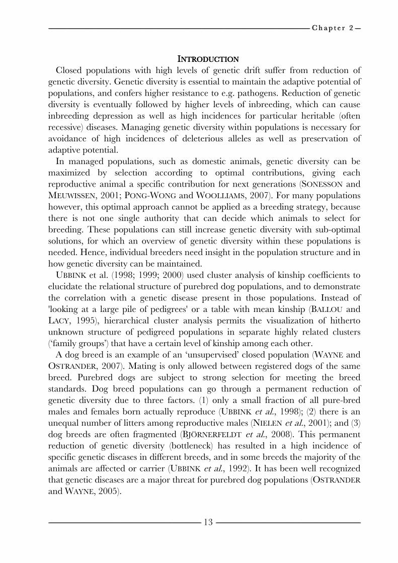
IIIINTRODUCTIONNTRODUCTIONNTRODUCTIONNTRODUCTION Closed populations with high levels of genetic drift suffer from reduction of
genetic diversity. Genetic diversity is essential to maintain the adaptive potential of populations, and confers higher resistance to e.g. pathogens. Reduction of genetic diversity is eventually followed by higher levels of inbreeding, which can cause inbreeding depression as well as high incidences for particular heritable (often recessive) diseases. Managing genetic diversity within populations is necessary for avoidance of high incidences of deleterious alleles as well as preservation of adaptive potential.
In managed populations, such as domestic animals, genetic diversity can be maximized by selection according to optimal contributions, giving each reproductive animal a specific contribution for next generations (SONESSON and MEUWISSEN, 2001; PONG-WONG and WOOLLIAMS, 2007). For many populations however, this optimal approach cannot be applied as a breeding strategy, because there is not one single authority that can decide which animals to select for breeding. These populations can still increase genetic diversity with sub-optimal solutions, for which an overview of genetic diversity within these populations is needed. Hence, individual breeders need insight in the population structure and in how genetic diversity can be maintained.
UBBINK et al. (1998; 1999; 2000) used cluster analysis of kinship coefficients to elucidate the relational structure of purebred dog populations, and to demonstrate the correlation with a genetic disease present in those populations. Instead of 'looking at a large pile of pedigrees' or a table with mean kinship (BALLOU and LACY, 1995), hierarchical cluster analysis permits the visualization of hitherto unknown structure of pedigreed populations in separate highly related clusters (‘family groups’) that have a certain level of kinship among each other.
A dog breed is an example of an ‘unsupervised’ closed population (WAYNE and OSTRANDER, 2007). Mating is only allowed between registered dogs of the same breed. Purebred dogs are subject to strong selection for meeting the breed standards. Dog breed populations can go through a permanent reduction of genetic diversity due to three factors. (1) only a small fraction of all pure-bred males and females born actually reproduce (UBBINK et al., 1998); (2) there is an unequal number of litters among reproductive males (NIELEN et al., 2001); and (3) dog breeds are often fragmented (BJÖRNERFELDT et al., 2008). This permanent reduction of genetic diversity (bottleneck) has resulted in a high incidence of specific genetic diseases in different breeds, and in some breeds the majority of the animals are affected or carrier (UBBINK et al., 1992). It has been well recognized that genetic diseases are a major threat for purebred dog populations (OSTRANDER and WAYNE, 2005).
-------------------- C l u s t e r a n a l y s i s r e v e a l s d i v e r s i t y C l u s t e r a n a l y s i s r e v e a l s d i v e r s i t y C l u s t e r a n a l y s i s r e v e a l s d i v e r s i t y C l u s t e r a n a l y s i s r e v e a l s d i v e r s i t y ----------------------------------------------------------------------------------------------------------------------------------------------------------------------------------------------------------------------------------------------------------------------------------------------------------------------------------------------------------------------------------------------------------------------------------------------------------------------------------------------------------------------------------------------------------------------------------------------------------------------------------------------------------------
-------------------------------------------------------------------------------------------------------------------------------------------------------------------------------------------------------------------------------------------------------------------------------------------------------------------------------------------------------------------------------------------------------------------------------------------------------------------------------------------------------------------------------------------------------------------------------------------------------------------------------------------- ----------------------------------------------------------------------------------------------------------------------------------------------------------------------------------------------------------------------------------------------------------------------------------------------------------------------------------------------------------------------------------------------------------------------------------------------------------------------------------------------------------------------------------------------------------------------------------------------------------------
14
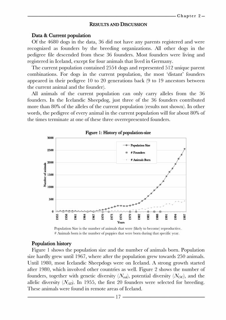
Icelandic Sheepdogs are bred in several European countries by many individual breeders. It is well known that the current population descends almost entirely from only few founders that were selected from remote areas in Iceland between 1955 and 1965.
This research investigates the amount of genetic diversity lost and the possibilities to maintain or increase genetic diversity within the Icelandic Sheepdog as a typical closed dog population. Furthermore, the use of cluster analysis is evaluated as a tool as well as its potential to identify genetic diversity.
MMMMETHODSETHODSETHODSETHODS
DataDataDataData We received pedigree data via Icelandic Sheepdog International Committee
(ISIC) of the population of Icelandic Sheepdogs in the following countries: the Netherlands (725 records), Sweden (1367), Iceland (1654), Germany (153), Norway (774), Denmark (2241) and Finland (113). Pedigree data contained unique ID, father, mother, gender, date of birth, country of birth, and occasionally date of death. Only Iceland had data since 1955. Other countries started breeding since 1975 or later. Most data were until 2002, but some were until 1998. Except for a few dogs in France, these countries contained the entire global Icelandic Sheepdog population. Pedigree data per country overlapped. The pedigree data were assembled into a single database table, and animals that were recorded twice were removed by information on country of birth. Animals without recorded parents were classified as either a true founder: animal without relationship with other founders, or an ‘animal with unknown parents’: an animal that descend from founders or their progeny, but having unknown parentage. All original founders were documented by the kennel clubs. No true founders descended from any of the other founders. By connecting data from each country, all parents for each related animal with unknown parents were found, leaving only true founders without known parents. Until 1998 pedigrees were complete for all countries. A general life expectancy progeny for females and males separately was estimated from the interval between date of birth of parents and. If date of death was not recorded, it was estimated by the life expectancy. All animals born in the years 1991 to 1998 were regarded as the ‘current-population’.
Population Diversity MeasuresPopulation Diversity MeasuresPopulation Diversity MeasuresPopulation Diversity Measures Unless stated differently, inbreeding and kinship coefficients were calculated
using the tabular method. Mean kinship was proposed by BALLOU and LACY (1995) and is the mean of the kinship coefficients between that individual and all reproductive individuals of the current population (candidates) including the individual itself. The mean kinship (mki) for individual i is calculated by BALLOU and LACY (1995):
------------------------------------------------------------------------------------------------------------------------------------------------------------------------------------------------------------------------------------------------------------------------------------------------------------------------------------------------------------------------------------------------------------------------------------------------------------------------------------------------------------------------------------------------------------------------------------------------------------------------------------------------------------------------------------------------------------------------------------------------------------------------------------------------------------------------------------------------------------------------------------------------------------------------------------------------------------------------------------------------------------------------------------------------------------------------------------------------ C h a p t e r C h a p t e r C h a p t e r C h a p t e r 2222 --------------------
---------------------------------------------------------------------------------------------------------------------------------------------------------------------------------------------------------------------------------------------------------------------------------------------------------------------------------------------------------------------------------------------------------------------------------------------------------------------------------------------------------------------------------------------------------------------------------------------------------------------------------------- --------------------------------------------------------------------------------------------------------------------------------------------------------------------------------------------------------------------------------------------------------------------------------------------------------------------------------------------------------------------------------------------------------------------------------------------------------------------------------------------------------------------------------------------------------------------------------------------------------
15
∑=
=�
j
iji f�
mk1
1,, ((11))
where N is the number of candidates and ƒij is the kinship between individual i an individual j. The mean kinship of an animal is a measure of the genetic importance of that individual within a population; animals with low mean kinship are more valuable for genetic diversity. Mean kinship depends on the population. From this follows that mean kinship of an animal might change over time when a population changes. Within conservation genetics, mean kinship is an important tool to maintain genetic diversity (FRANKHAM et al., 2002).
The following population diversity measures were used: Average inbreeding (F ) is the average of inbreeding coefficient of all candidates.
F indicates the current risk of inbreeding depression in the current population. Average mean kinship (mk ) is the average of mean kinships of all candidates
within the population under study (BALLOU and LACY, 1995):
∑∑∑= ==
==�
i
�
j
ij
�
i
i f�
mk�
mk1 1
21
11,, ((22))
Average mean kinship differs from average pairwise kinship because mk comprises kinship of animals with itself.
In this research genetic diversity (Nmk) is defined as the number of equally contributing founders with no random loss of founder alleles in descendants that would be expected to produce the same average mean kinship (and therefore genetic variation) as in the population under study. Nmk is mk expressed on the scale of founder genome equivalents (LACY, 1989; CABALLERO and TORO, 2000) and is calculated by Nmk=1/2mk . Lower average mean kinship signifies higher genetic diversity and thus a higher capacity to adapt as a population.
In this research allelic diversity (NAD) is defined as half the number of distinct alleles that is still present in the population under study if all founder alleles would be unique. The number of unique founder alleles that survived each year was determined by a genedrop (LACY, 1995), which was repeated 10.000 times. NAD is also expressed in founder genome equivalents and can therefore be compared with Nmk and NOC (see below). For example, if frequencies of all alleles were equal, NAD would be equal to Nmk. NAD monitors the loss of genetic diversity due to extinction of unique (founder-) alleles.
In this research potential diversity (NOC) is defined as the maximum genetic diversity the population under study can achieve (expressed in founder genome equivalents). NOC is the genetic diversity obtained when average mean kinship is minimized using Optimal Contribution Selection. NOC is calculated as described in GENERAL INTRODUCTION (Chapter 1):
OCOC
OCmk
�Fc'c*2
1
2
1
min
== ,, ((33))
where FFFF is a matrix of kinships between all individuals, including kinship of individuals with themselves, and ccccOC is a column vector of proportional
-------------------- C l u s t e r a n a l y s i s r e v e a l s d i v e r s i t y C l u s t e r a n a l y s i s r e v e a l s d i v e r s i t y C l u s t e r a n a l y s i s r e v e a l s d i v e r s i t y C l u s t e r a n a l y s i s r e v e a l s d i v e r s i t y ----------------------------------------------------------------------------------------------------------------------------------------------------------------------------------------------------------------------------------------------------------------------------------------------------------------------------------------------------------------------------------------------------------------------------------------------------------------------------------------------------------------------------------------------------------------------------------------------------------------------------------------------------------------
-------------------------------------------------------------------------------------------------------------------------------------------------------------------------------------------------------------------------------------------------------------------------------------------------------------------------------------------------------------------------------------------------------------------------------------------------------------------------------------------------------------------------------------------------------------------------------------------------------------------------------------------- ----------------------------------------------------------------------------------------------------------------------------------------------------------------------------------------------------------------------------------------------------------------------------------------------------------------------------------------------------------------------------------------------------------------------------------------------------------------------------------------------------------------------------------------------------------------------------------------------------------------
16
contributions of individuals to the next generation, so that the sum of elements of ccccOC equals one and minimizes ccccOC’Fc’Fc’Fc’FcOC (MEUWISSEN, 1997). ccccOC is given by EDING et al. (2002):
1F1'
1Fc
1
1
−
−
=OC,, ((44))
where 1111 is a column vector of ones. ccccOC contains contributions of parents to next generations that would minimize mk in next generations. ccccOC calculated from Equation 4, however, can contain negative contributions, which is impossible in practice. When negative contributions were obtained, the most negative contribution was set to zero and vector ccccOC was recalculated until all contributions were non-negative. NOC is the highest possible Nmk and measures the diversity that could be obtained in next generations. NOC will always be equal or higher than Nmk and equal or lower than NAD. NOC is relevant within closed populations, since the population can never get higher diversity than NOC. Therefore, it monitors the unrestorable loss of genetic diversity.
Diversity and Population HistoryDiversity and Population HistoryDiversity and Population HistoryDiversity and Population History Each year a ‘current population’ was determined by animals that were
reproductive plus (young) animals that still could become reproductive in future years. For each year, the following population-parameters were determined: the current population size; the number of progeny born during that year; the number of founder introductions; and the following diversity measures: F , mk , Nmk, NOC, NAD (as described above).
ClusterClusterClusterCluster----analysisanalysisanalysisanalysis Cluster-analysis was performed twice on the current population. (1) The first
analysis was based on kinship calculated using the tabular method starting with the founders. Next, UPGMA clustered all animals (SNEATH and SOKAL, 1973). Since the level of kinship to delimit family groups is arbitrary, the ‘cut-off level’ of kinship was done in a way that ten clusters were obtained. The selection of ten clusters was decided based on considerations of displaying. The clusters were displayed in a dendrogram, which is referred to as the all-gen-tree. (2) The second cluster-analysis was performed as described by UBBINK et al. (1998). Kinship between all animals was calculated by the path method (WRIGHT, 1922) until seven generations backwards (instead of tabular method that includes all generations). Note that if the path method would include all generations, results would be equal to the tabular method. Next, all animals were clustered using UPGMA. Subsequently all clusters having an average mean kinship greater/equal to 0.0625 were defined as the final clusters and displayed in a dendrogram. This kinship value of 0.0625 that delimits clusters corresponds with kinship between second degree cousins and was used by UBBINK et al. (1998). This dendrogram is referred to as the 7-gen-tree.
------------------------------------------------------------------------------------------------------------------------------------------------------------------------------------------------------------------------------------------------------------------------------------------------------------------------------------------------------------------------------------------------------------------------------------------------------------------------------------------------------------------------------------------------------------------------------------------------------------------------------------------------------------------------------------------------------------------------------------------------------------------------------------------------------------------------------------------------------------------------------------------------------------------------------------------------------------------------------------------------------------------------------------------------------------------------------------------------ C h a p t e r C h a p t e r C h a p t e r C h a p t e r 2222 --------------------
---------------------------------------------------------------------------------------------------------------------------------------------------------------------------------------------------------------------------------------------------------------------------------------------------------------------------------------------------------------------------------------------------------------------------------------------------------------------------------------------------------------------------------------------------------------------------------------------------------------------------------------- --------------------------------------------------------------------------------------------------------------------------------------------------------------------------------------------------------------------------------------------------------------------------------------------------------------------------------------------------------------------------------------------------------------------------------------------------------------------------------------------------------------------------------------------------------------------------------------------------------
17
RRRRESULTS AND ESULTS AND ESULTS AND ESULTS AND DDDDISCUSSIONISCUSSIONISCUSSIONISCUSSION
Data & Current populationData & Current populationData & Current populationData & Current population Of the 4680 dogs in the data, 36 did not have any parents registered and were
recognized as founders by the breeding organizations. All other dogs in the pedigree file descended from these 36 founders. Most founders were living and registered in Iceland, except for four animals that lived in Germany.
The current population contained 2554 dogs and represented 512 unique parent combinations. For dogs in the current population, the most ‘distant’ founders appeared in their pedigree 10 to 20 generations back (9 to 19 ancestors between the current animal and the founder).
All animals of the current population can only carry alleles from the 36 founders. In the Icelandic Sheepdog, just three of the 36 founders contributed more than 80% of the alleles of the current population (results not shown). In other words, the pedigree of every animal in the current population will for about 80% of the times terminate at one of these three overrepresented founders.
Figure 1: History of populationFigure 1: History of populationFigure 1: History of populationFigure 1: History of population----size size size size
Population Size is the number of animals that were (likely to become) reproductive. # Animals born is the number of puppies that were born during that specific year.
Population historyPopulation historyPopulation historyPopulation history Figure 1 shows the population size and the number of animals born. Population
size hardly grew until 1967, where after the population grew towards 250 animals. Until 1980, most Icelandic Sheepdogs were on Iceland. A strong growth started after 1980, which involved other countries as well. Figure 2 shows the number of founders, together with genetic diversity (Nmk), potential diversity (NOC), and the allelic diversity (NAD). In 1955, the first 20 founders were selected for breeding. These animals were found in remote areas of Iceland.
0000
500500500500
1000100010001000
1500150015001500
2000200020002000
2500250025002500
3000300030003000
1955
1955
1955
1955
1958
1958
1958
1958
1961
1961
1961
1961
1964
1964
1964
1964
1967
1967
1967
1967
1970
1970
1970
1970
1973
1973
1973
1973
1976
1976
1976
1976
1979
1979
1979
1979
1982
1982
1982
1982
1985
1985
1985
1985
1988
1988
1988
1988
1991
1991
1991
1991
1994
1994
1994
1994
1997
1997
1997
1997
YearsYearsYearsYears
Num
ber
of a
nim
als
Num
ber
of a
nim
als
Num
ber
of a
nim
als
Num
ber
of a
nim
als
Population SizePopulation SizePopulation SizePopulation Size
# Founders# Founders# Founders# Founders
# Animals Born# Animals Born# Animals Born# Animals Born
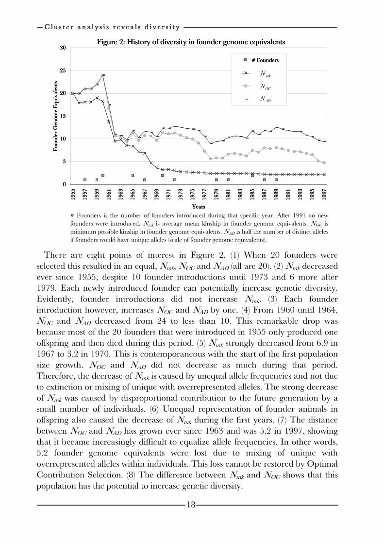
-------------------- C l u s t e r a n a l y s i s r e v e a l s d i v e r s i t y C l u s t e r a n a l y s i s r e v e a l s d i v e r s i t y C l u s t e r a n a l y s i s r e v e a l s d i v e r s i t y C l u s t e r a n a l y s i s r e v e a l s d i v e r s i t y ----------------------------------------------------------------------------------------------------------------------------------------------------------------------------------------------------------------------------------------------------------------------------------------------------------------------------------------------------------------------------------------------------------------------------------------------------------------------------------------------------------------------------------------------------------------------------------------------------------------------------------------------------------------
-------------------------------------------------------------------------------------------------------------------------------------------------------------------------------------------------------------------------------------------------------------------------------------------------------------------------------------------------------------------------------------------------------------------------------------------------------------------------------------------------------------------------------------------------------------------------------------------------------------------------------------------- ----------------------------------------------------------------------------------------------------------------------------------------------------------------------------------------------------------------------------------------------------------------------------------------------------------------------------------------------------------------------------------------------------------------------------------------------------------------------------------------------------------------------------------------------------------------------------------------------------------------
18
Figure 2: History of diversity in founder genome equivalentsFigure 2: History of diversity in founder genome equivalentsFigure 2: History of diversity in founder genome equivalentsFigure 2: History of diversity in founder genome equivalents
There are eight points of interest in Figure 2. (1) When 20 founders were
selected this resulted in an equal, Nmk, NOC and NAD (all are 20). (2) Nmk decreased ever since 1955, despite 10 founder introductions until 1973 and 6 more after 1979. Each newly introduced founder can potentially increase genetic diversity. Evidently, founder introductions did not increase Nmk. (3) Each founder introduction however, increases NOC and NAD by one. (4) From 1960 until 1964, NOC and NAD decreased from 24 to less than 10. This remarkable drop was because most of the 20 founders that were introduced in 1955 only produced one offspring and then died during this period. (5) Nmk strongly decreased from 6.9 in 1967 to 3.2 in 1970. This is contemporaneous with the start of the first population size growth. NOC and NAD did not decrease as much during that period. Therefore, the decrease of Nmk is caused by unequal allele frequencies and not due to extinction or mixing of unique with overrepresented alleles. The strong decrease of Nmk was caused by disproportional contribution to the future generation by a small number of individuals. (6) Unequal representation of founder animals in offspring also caused the decrease of Nmk during the first years. (7) The distance between NOC and NAD has grown ever since 1963 and was 5.2 in 1997, showing that it became increasingly difficult to equalize allele frequencies. In other words, 5.2 founder genome equivalents were lost due to mixing of unique with overrepresented alleles within individuals. This loss cannot be restored by Optimal Contribution Selection. (8) The difference between Nmk and NOC shows that this population has the potential to increase genetic diversity.
0000
5555
10101010
15151515
20202020
25252525
30303030
1955
1955
1955
1955
1957
1957
1957
1957
1959
1959
1959
1959
1961
1961
1961
1961
1963
1963
1963
1963
1965
1965
1965
1965
1967
1967
1967
1967
1969
1969
1969
1969
1971
1971
1971
1971
1973
1973
1973
1973
1975
1975
1975
1975
1977
1977
1977
1977
1979
1979
1979
1979
1981
1981
1981
1981
1983
1983
1983
1983
1985
1985
1985
1985
1987
1987
1987
1987
1989
1989
1989
1989
1991
1991
1991
1991
1993
1993
1993
1993
1995
1995
1995
1995
1997
1997
1997
1997
YearsYearsYearsYears
Fou
nder
Gen
ome
Equ
ival
ents
Fou
nder
Gen
ome
Equ
ival
ents
Fou
nder
Gen
ome
Equ
ival
ents
Fou
nder
Gen
ome
Equ
ival
ents
# Founders# Founders# Founders# Founders
mk�
OC�
AD�
# Founders is the number of founders introduced during that specific year. After 1991 no new founders were introduced. Nmk is average mean kinship in founder genome equivalents. NOC is minimum possible kinship in founder genome equivalents. NAD is half the number of distinct alleles if founders would have unique alleles (scale of founder genome equivalents).
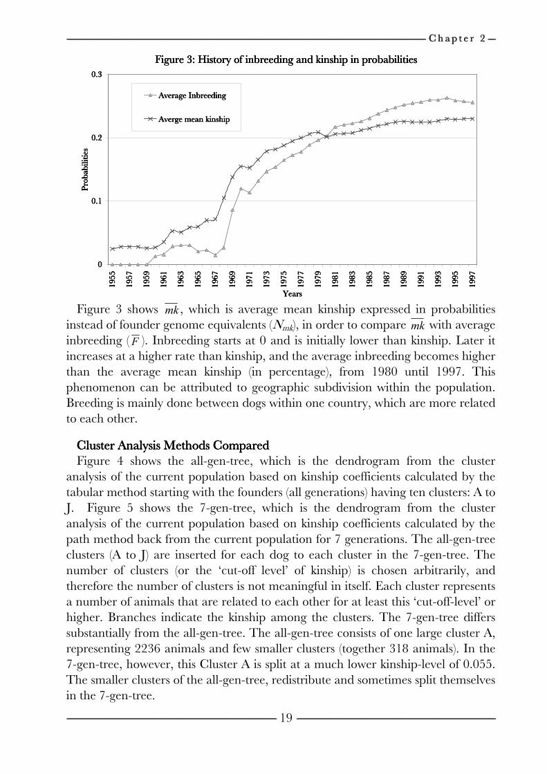
------------------------------------------------------------------------------------------------------------------------------------------------------------------------------------------------------------------------------------------------------------------------------------------------------------------------------------------------------------------------------------------------------------------------------------------------------------------------------------------------------------------------------------------------------------------------------------------------------------------------------------------------------------------------------------------------------------------------------------------------------------------------------------------------------------------------------------------------------------------------------------------------------------------------------------------------------------------------------------------------------------------------------------------------------------------------------------------------ C h a p t e r C h a p t e r C h a p t e r C h a p t e r 2222 --------------------
---------------------------------------------------------------------------------------------------------------------------------------------------------------------------------------------------------------------------------------------------------------------------------------------------------------------------------------------------------------------------------------------------------------------------------------------------------------------------------------------------------------------------------------------------------------------------------------------------------------------------------------- --------------------------------------------------------------------------------------------------------------------------------------------------------------------------------------------------------------------------------------------------------------------------------------------------------------------------------------------------------------------------------------------------------------------------------------------------------------------------------------------------------------------------------------------------------------------------------------------------------
19
Figure 3: History of inbreeding and kinship in probabilities Figure 3: History of inbreeding and kinship in probabilities Figure 3: History of inbreeding and kinship in probabilities Figure 3: History of inbreeding and kinship in probabilities
Figure 3 shows mk , which is average mean kinship expressed in probabilities
instead of founder genome equivalents (Nmk), in order to compare mk with average inbreeding (F ). Inbreeding starts at 0 and is initially lower than kinship. Later it increases at a higher rate than kinship, and the average inbreeding becomes higher than the average mean kinship (in percentage), from 1980 until 1997. This phenomenon can be attributed to geographic subdivision within the population. Breeding is mainly done between dogs within one country, which are more related to each other.
Cluster Analysis Cluster Analysis Cluster Analysis Cluster Analysis Methods ComparedMethods ComparedMethods ComparedMethods Compared Figure 4 shows the all-gen-tree, which is the dendrogram from the cluster
analysis of the current population based on kinship coefficients calculated by the tabular method starting with the founders (all generations) having ten clusters: A to J. Figure 5 shows the 7-gen-tree, which is the dendrogram from the cluster analysis of the current population based on kinship coefficients calculated by the path method back from the current population for 7 generations. The all-gen-tree clusters (A to J) are inserted for each dog to each cluster in the 7-gen-tree. The number of clusters (or the ‘cut-off level’ of kinship) is chosen arbitrarily, and therefore the number of clusters is not meaningful in itself. Each cluster represents a number of animals that are related to each other for at least this ‘cut-off-level’ or higher. Branches indicate the kinship among the clusters. The 7-gen-tree differs substantially from the all-gen-tree. The all-gen-tree consists of one large cluster A, representing 2236 animals and few smaller clusters (together 318 animals). In the 7-gen-tree, however, this Cluster A is split at a much lower kinship-level of 0.055. The smaller clusters of the all-gen-tree, redistribute and sometimes split themselves in the 7-gen-tree.
0000
0.10.10.10.1
0.20.20.20.2
0.30.30.30.3
1955
1955
1955
1955
1957
1957
1957
1957
1959
1959
1959
1959
1961
1961
1961
1961
1963
1963
1963
1963
1965
1965
1965
1965
1967
1967
1967
1967
1969
1969
1969
1969
1971
1971
1971
1971
1973
1973
1973
1973
1975
1975
1975
1975
1977
1977
1977
1977
1979
1979
1979
1979
1981
1981
1981
1981
1983
1983
1983
1983
1985
1985
1985
1985
1987
1987
1987
1987
1989
1989
1989
1989
1991
1991
1991
1991
1993
1993
1993
1993
1995
1995
1995
1995
1997
1997
1997
1997
YearsYearsYearsYears
Pro
babi
litie
sP
roba
bilit
ies
Pro
babi
litie
sP
roba
bilit
ies
Average InbreedingAverage InbreedingAverage InbreedingAverage Inbreeding
Averge mean kinshipAverge mean kinshipAverge mean kinshipAverge mean kinship
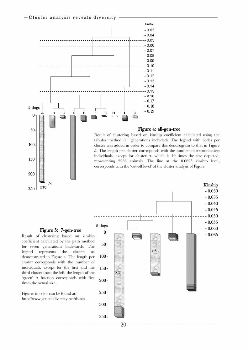
Result of clustering based on kinship coefficient calculated by the path method for seven generations backwards. The legend represents the clusters as demonstrated in Figure 4. The length per cluster corresponds windividuals, except for the first and the third cluster from the left: the length of the ‘green’ A fraction corresponds with five times the actual size. Figures in color can be found at:http://www.geneticdiversity.net/thesis/
-------------------- C l u s t e r a n a l y s i s r e v e a l s d i v e r s i t y C l u s t e r a n a l y s i s r e v e a l s d i v e r s i t y C l u s t e r a n a l y s i s r e v e a l s d i v e r s i t y C l u s t e r a n a l y s i s r e v e a l s d i v e r s i t y
----------------------------------------------------------------------------------------------------------------------------------------------------------------------------------------------------------------------------------------------------------------------------------------------------------------------------------------------------------------------------------------------------------------------------------------------------------------------------------------
Figure 5: Figure 5: Figure 5: Figure 5: Result of clustering based on kinship coefficient calculated by the path method for seven generations backwards. The legend represents the clusters as demonstrated in Figure 4. The length per cluster corresponds windividuals, except for the first and the third cluster from the left: the length of the ‘green’ A fraction corresponds with five times the actual size. Figures in color can be found at:http://www.geneticdiversity.net/thesis/
C l u s t e r a n a l y s i s r e v e a l s d i v e r s i t y C l u s t e r a n a l y s i s r e v e a l s d i v e r s i t y C l u s t e r a n a l y s i s r e v e a l s d i v e r s i t y C l u s t e r a n a l y s i s r e v e a l s d i v e r s i t y
----------------------------------------------------------------------------------------------------------------------------------------------------------------------------------------------------------------------------------------------------------------------------------------------------------------------------------------------------------------------------------------------------------------------------------------------------------------------------------------
Figure 5: Figure 5: Figure 5: Figure 5: 7777----gengengengenResult of clustering based on kinship coefficient calculated by the path method for seven generations backwards. The legend represents the clusters as demonstrated in Figure 4. The length per cluster corresponds with the number of individuals, except for the first and the third cluster from the left: the length of the ‘green’ A fraction corresponds with five times the actual size.
Figures in color can be found at:http://www.geneticdiversity.net/thesis/
C l u s t e r a n a l y s i s r e v e a l s d i v e r s i t y C l u s t e r a n a l y s i s r e v e a l s d i v e r s i t y C l u s t e r a n a l y s i s r e v e a l s d i v e r s i t y C l u s t e r a n a l y s i s r e v e a l s d i v e r s i t y
----------------------------------------------------------------------------------------------------------------------------------------------------------------------------------------------------------------------------------------------------------------------------------------------------------------------------------------------------------------------------------------------------------------------------------------------------------------------------------------
gengengengen----tree tree tree tree Result of clustering based on kinship coefficient calculated by the path method for seven generations backwards. The legend represents the clusters as demonstrated in Figure 4. The length per
ith the number of individuals, except for the first and the third cluster from the left: the length of the ‘green’ A fraction corresponds with five
Figures in color can be found at: http://www.geneticdiversity.net/thesis/
C l u s t e r a n a l y s i s r e v e a l s d i v e r s i t y C l u s t e r a n a l y s i s r e v e a l s d i v e r s i t y C l u s t e r a n a l y s i s r e v e a l s d i v e r s i t y C l u s t e r a n a l y s i s r e v e a l s d i v e r s i t y
----------------------------------------------------------------------------------------------------------------------------------------------------------------------------------------------------------------------------------------------------------------------------------------------------------------------------------------------------------------------------------------------------------------------------------------------------------------------------------------------------------------------------------------------------------------------------------------------------------------
Result of clustering based on kinship coefficient calculated by the path method for seven generations backwards. The legend represents the clusters as demonstrated in Figure 4. The length per
ith the number of individuals, except for the first and the third cluster from the left: the length of the ‘green’ A fraction corresponds with five
Result of clustering based on kinship coefficient calculated using the tabular method (all generations included). The legend with codes per cluster was added in order to compare this dendrogram to that in Figure 5. The length per cluster corresponds with the number of (reproductive) individuals, except for cluster A, which is 10 times the size depicted, representing 2236 animals. The line at the 0.0625 kinship level, corresponds with the ‘cut
C l u s t e r a n a l y s i s r e v e a l s d i v e r s i t y C l u s t e r a n a l y s i s r e v e a l s d i v e r s i t y C l u s t e r a n a l y s i s r e v e a l s d i v e r s i t y C l u s t e r a n a l y s i s r e v e a l s d i v e r s i t y ------------------------------------------------------------------------------------------------------------------------------------------------------------------------------------------------------------------------------------------------------------------------------------------------------------------------------------------------------------------------------------------------------------------------------------------------------------------------------------------------------------------------------------------------------------
---------------------------------------------------------------------------------------------------------------------------------------------------- --------------------------------------------------------------------------------------------------------------------------------------------------------------------------------------------------------------------------------20
Result of clustering based on kinship coefficient calculated using the tabular method (all generations included). The legend with codes per cluster was added in order to compare this dendrogram to that in Figure
length per cluster corresponds with the number of (reproductive) individuals, except for cluster A, which is 10 times the size depicted, representing 2236 animals. The line at the 0.0625 kinship level, corresponds with the ‘cut
--------------------------------------------------------------------------------------------------------------------------------------------------------------------------------------------------------------------------------------------------------------------------------------------------------------------------------------------------------------------------------------------------------------------------------------------------------------------------------------------------------------------
--------------------------------------------------------------------------------------------------------------------------------------------------------------------------------------------------------------------------------
Figure Figure Figure Figure 4444: : : : Result of clustering based on kinship coefficient calculated using the tabular method (all generations included). The legend with codes per cluster was added in order to compare this dendrogram to that in Figure
length per cluster corresponds with the number of (reproductive) individuals, except for cluster A, which is 10 times the size depicted, representing 2236 animals. The line at the 0.0625 kinship level, corresponds with the ‘cut-off level’ of the cluster an
--------------------------------------------------------------------------------------------------------------------------------------------------------------------------------------------------------------------------------------------------------------------------------------------------------------------------------------------------------------------------------------------------------------------------------------------------------------------------------------------------------------------
----------------------------------------------------------------------------------------------------------------------------------------------------------------------------------------------------------------------------------------------------------------------------------------------------------------------------------------------------------------------------------------------------------------------------------------------------------------------------------------------------------------------------------------------------------------------------------------------------------------
: : : : allallallall----gengengengen----tree tree tree tree Result of clustering based on kinship coefficient calculated using the tabular method (all generations included). The legend with codes per cluster was added in order to compare this dendrogram to that in Figure
length per cluster corresponds with the number of (reproductive) individuals, except for cluster A, which is 10 times the size depicted, representing 2236 animals. The line at the 0.0625 kinship level,
off level’ of the cluster an
------------------------------------------------------------------------------------------------------------------------------------------------------------------------------------------------------------------------------------------------------------------------------------------------------------------------------------------------------------------------------------------------------------------------------------------------------------------------------------------------------------------------------------------------------------------------------------------------------------------------
--------------------------------------------------------------------------------------------------------------------------------------------------------------------------------------------------------------------------------------------------------------------------------------------
tree tree tree tree Result of clustering based on kinship coefficient calculated using the tabular method (all generations included). The legend with codes per cluster was added in order to compare this dendrogram to that in Figure
length per cluster corresponds with the number of (reproductive) individuals, except for cluster A, which is 10 times the size depicted, representing 2236 animals. The line at the 0.0625 kinship level,
off level’ of the cluster analysis of Figure
------------------------------------------------------------------------------------------------------------------------------------------------------------------------------------------------------------------------------------------------------------------------------------------------------------------------------------------------------------------------------------------------------------------------------------------------------------------------------------------------------------------------------------------------------------------------------------------------------------------------
--------------------------------------------------------------------------------------------------------------------------------------------------------------------------------------------------------------------------------------------------------------------------------------------
Result of clustering based on kinship coefficient calculated using the tabular method (all generations included). The legend with codes per cluster was added in order to compare this dendrogram to that in Figure
length per cluster corresponds with the number of (reproductive) individuals, except for cluster A, which is 10 times the size depicted, representing 2236 animals. The line at the 0.0625 kinship level,
alysis of Figure
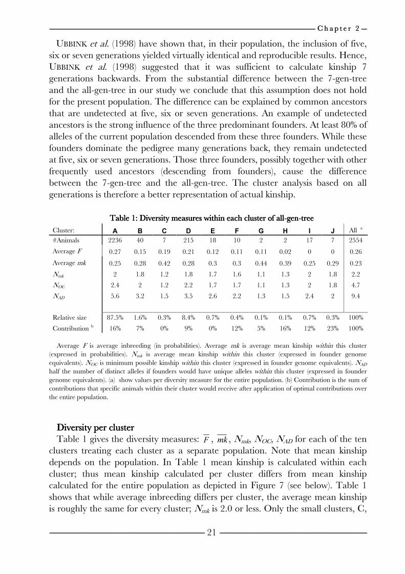
------------------------------------------------------------------------------------------------------------------------------------------------------------------------------------------------------------------------------------------------------------------------------------------------------------------------------------------------------------------------------------------------------------------------------------------------------------------------------------------------------------------------------------------------------------------------------------------------------------------------------------------------------------------------------------------------------------------------------------------------------------------------------------------------------------------------------------------------------------------------------------------------------------------------------------------------------------------------------------------------------------------------------------------------------------------------------------------------ C h a p t e r C h a p t e r C h a p t e r C h a p t e r 2222 --------------------
---------------------------------------------------------------------------------------------------------------------------------------------------------------------------------------------------------------------------------------------------------------------------------------------------------------------------------------------------------------------------------------------------------------------------------------------------------------------------------------------------------------------------------------------------------------------------------------------------------------------------------------- --------------------------------------------------------------------------------------------------------------------------------------------------------------------------------------------------------------------------------------------------------------------------------------------------------------------------------------------------------------------------------------------------------------------------------------------------------------------------------------------------------------------------------------------------------------------------------------------------------
21
UBBINK et al. (1998) have shown that, in their population, the inclusion of five, six or seven generations yielded virtually identical and reproducible results. Hence, UBBINK et al. (1998) suggested that it was sufficient to calculate kinship 7 generations backwards. From the substantial difference between the 7-gen-tree and the all-gen-tree in our study we conclude that this assumption does not hold for the present population. The difference can be explained by common ancestors that are undetected at five, six or seven generations. An example of undetected ancestors is the strong influence of the three predominant founders. At least 80% of alleles of the current population descended from these three founders. While these founders dominate the pedigree many generations back, they remain undetected at five, six or seven generations. Those three founders, possibly together with other frequently used ancestors (descending from founders), cause the difference between the 7-gen-tree and the all-gen-tree. The cluster analysis based on all generations is therefore a better representation of actual kinship.
Table 1: Diversity measures within each cluster of allTable 1: Diversity measures within each cluster of allTable 1: Diversity measures within each cluster of allTable 1: Diversity measures within each cluster of all----gengengengen----treetreetreetree
Cluster: A B C D E F G H I J All a
#Animals 2236 40 7 215 18 10 2 2 17 7 2554
Average F 0.27 0.15 0.19 0.21 0.12 0.11 0.11 0.02 0 0 0.26
Average mk 0.25 0.28 0.42 0.28 0.3 0.3 0.44 0.39 0.25 0.29 0.23
Nmk 2 1.8 1.2 1.8 1.7 1.6 1.1 1.3 2 1.8 2.2
NOC 2.4 2 1.2 2.2 1.7 1.7 1.1 1.3 2 1.8 4.7
NAD 5.6 3.2 1.5 3.5 2.6 2.2 1.3 1.5 2.4 2 9.4
Relative size 87.5% 1.6% 0.3% 8.4% 0.7% 0.4% 0.1% 0.1% 0.7% 0.3% 100%
Contribution b 16% 7% 0% 9% 0% 12% 5% 16% 12% 23% 100% Average F is average inbreeding (in probabilities). Average mk is average mean kinship within this cluster
(expressed in probabilities). Nmk is average mean kinship within this cluster (expressed in founder genome equivalents). NOC is minimum possible kinship within this cluster (expressed in founder genome equivalents). NAD half the number of distinct alleles if founders would have unique alleles within this cluster (expressed in founder genome equivalents). (a) show values per diversity measure for the entire population. (b) Contribution is the sum of contributions that specific animals within their cluster would receive after application of optimal contributions over the entire population.
Diversity per clusterDiversity per clusterDiversity per clusterDiversity per cluster Table 1 gives the diversity measures: F , mk , Nmk, NOC, NAD for each of the ten
clusters treating each cluster as a separate population. Note that mean kinship depends on the population. In Table 1 mean kinship is calculated within each cluster; thus mean kinship calculated per cluster differs from mean kinship calculated for the entire population as depicted in Figure 7 (see below). Table 1 shows that while average inbreeding differs per cluster, the average mean kinship is roughly the same for every cluster; Nmk is 2.0 or less. Only the small clusters, C,
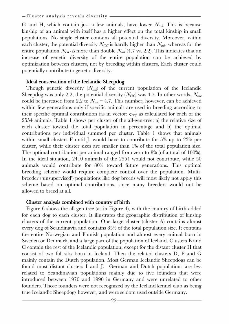
-------------------- C l u s t e r a n a l y s i s r e v e a l s d i v e r s i t y C l u s t e r a n a l y s i s r e v e a l s d i v e r s i t y C l u s t e r a n a l y s i s r e v e a l s d i v e r s i t y C l u s t e r a n a l y s i s r e v e a l s d i v e r s i t y ----------------------------------------------------------------------------------------------------------------------------------------------------------------------------------------------------------------------------------------------------------------------------------------------------------------------------------------------------------------------------------------------------------------------------------------------------------------------------------------------------------------------------------------------------------------------------------------------------------------------------------------------------------------
-------------------------------------------------------------------------------------------------------------------------------------------------------------------------------------------------------------------------------------------------------------------------------------------------------------------------------------------------------------------------------------------------------------------------------------------------------------------------------------------------------------------------------------------------------------------------------------------------------------------------------------------- ----------------------------------------------------------------------------------------------------------------------------------------------------------------------------------------------------------------------------------------------------------------------------------------------------------------------------------------------------------------------------------------------------------------------------------------------------------------------------------------------------------------------------------------------------------------------------------------------------------------
22
G and H, which contain just a few animals, have lower Nmk. This is because kinship of an animal with itself has a higher effect on the total kinship in small populations. No single cluster contains all potential diversity. Moreover, within each cluster, the potential diversity NOC is hardly higher than Nmk, whereas for the entire population NOC is more than double Nmk (4.7 vs. 2.2). This indicates that an increase of genetic diversity of the entire population can be achieved by optimization between clusters, not by breeding within clusters. Each cluster could potentially contribute to genetic diversity.
Ideal conservation of the Icelandic SheepdogIdeal conservation of the Icelandic SheepdogIdeal conservation of the Icelandic SheepdogIdeal conservation of the Icelandic Sheepdog Though genetic diversity (Nmk) of the current population of the Icelandic
Sheepdog was only 2.2, the potential diversity (NOC) was 4.7. In other words, Nmk could be increased from 2.2 to Nmk = 4.7. This number, however, can be achieved within few generations only if specific animals are used in breeding according to their specific optimal contribution (as in vector: ccccOC) as calculated for each of the 2554 animals. Table 1 shows per cluster of the all-gen-tree: a) the relative size of each cluster toward the total population in percentage and b) the optimal contributions per individual summed per cluster. Table 1 shows that animals within small clusters F until J, would have to contribute for 5% up to 23% per cluster, while their cluster sizes are smaller than 1% of the total population size. The optimal contribution per animal ranged from zero to 8% (of a total of 100%). In the ideal situation, 2410 animals of the 2554 would not contribute, while 50 animals would contribute for 80% toward future generations. This optimal breeding scheme would require complete control over the population. Multi-breeder (‘unsupervised’) populations like dog breeds will most likely not apply this scheme based on optimal contributions, since many breeders would not be allowed to breed at all.
Cluster analysis combined with country of birthCluster analysis combined with country of birthCluster analysis combined with country of birthCluster analysis combined with country of birth Figure 6 shows the all-gen-tree (as in Figure 4), with the country of birth added
for each dog to each cluster. It illustrates the geographic distribution of kinship clusters of the current population. One large cluster (cluster A) contains almost every dog of Scandinavia and contains 85% of the total population size. It contains the entire Norwegian and Finnish population and almost every animal born in Sweden or Denmark, and a large part of the population of Iceland. Clusters B and C contain the rest of the Icelandic population, except for the distant cluster H that consist of two full-sibs born in Iceland. Then the related clusters D, F and G mainly contain the Dutch population. Most German Icelandic Sheepdogs can be found most distant clusters I and J. German and Dutch populations are less related to Scandinavian populations mainly due to five founders that were introduced between 1970 and 1990 in Germany and were unrelated to other founders. Those founders were not recognized by the Iceland kennel club as being true Icelandic Sheepdogs however, and were seldom used outside Germany.
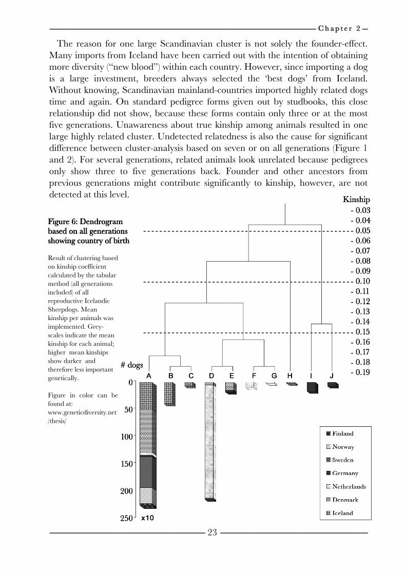
------------------------------------------------------------------------------------------------------------------------------------------------------------------------------------------------------------------------------------------------------------------------------------------------------------------------------------------------------------------------------------------------------------------------------------------------------------------------------------------------------------------------------------------------------------------------------------------------------------------------------------------------------------------------------------------------------------------------------------------------------------------------------------------------------------------------------------------------------------------------------------------------------------------------------------------------------------------------------------------------------------------------------------------------------------------------------------------------ C h a p t e r C h a p t e r C h a p t e r C h a p t e r 2222 --------------------
---------------------------------------------------------------------------------------------------------------------------------------------------------------------------------------------------------------------------------------------------------------------------------------------------------------------------------------------------------------------------------------------------------------------------------------------------------------------------------------------------------------------------------------------------------------------------------------------------------------------------------------- --------------------------------------------------------------------------------------------------------------------------------------------------------------------------------------------------------------------------------------------------------------------------------------------------------------------------------------------------------------------------------------------------------------------------------------------------------------------------------------------------------------------------------------------------------------------------------------------------------
23
The reason for one large Scandinavian cluster is not solely the founder-effect. Many imports from Iceland have been carried out with the intention of obtaining more diversity (“new blood”) within each country. However, since importing a dog is a large investment, breeders always selected the ‘best dogs’ from Iceland. Without knowing, Scandinavian mainland-countries imported highly related dogs time and again. On standard pedigree forms given out by studbooks, this close relationship did not show, because these forms contain only three or at the most five generations. Unawareness about true kinship among animals resulted in one large highly related cluster. Undetected relatedness is also the cause for significant difference between cluster-analysis based on seven or on all generations (Figure 1 and 2). For several generations, related animals look unrelated because pedigrees only show three to five generations back. Founder and other ancestors from previous generations might contribute significantly to kinship, however, are not detected at this level.
Result of clustering based on kinship coefficient calculated by the tabular method (all generations included) of all reproductive Icelandic Sheepdogs. Mean kinship per animals was implemented. Grey-scales indicate the mean kinship for each animal; higher mean kinships show darker and therefore less important genetically. Figure in color can be found at: www.geneticdiversity.net/thesis/
Figure 6: Dendrogram Figure 6: Dendrogram Figure 6: Dendrogram Figure 6: Dendrogram based on all generations based on all generations based on all generations based on all generations showing country of birthshowing country of birthshowing country of birthshowing country of birth
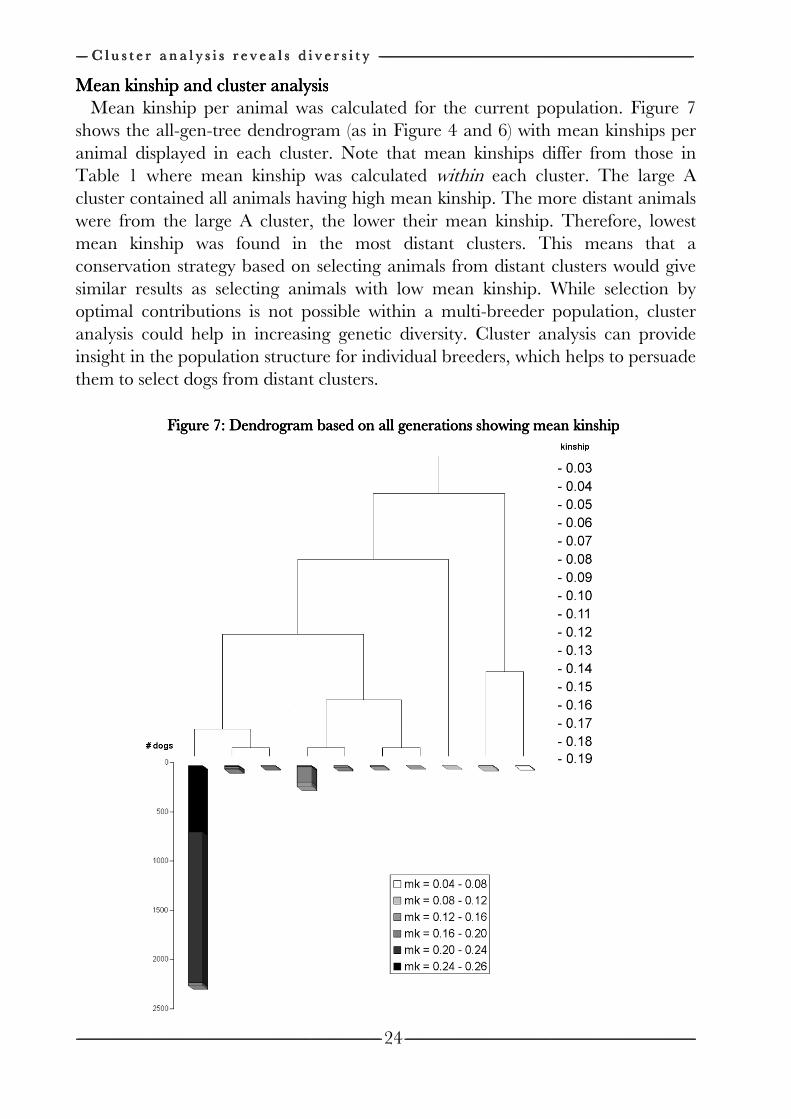
-------------------- C l u s t e r a n a l y s i s r e v e a l s d i v e r s i t y C l u s t e r a n a l y s i s r e v e a l s d i v e r s i t y C l u s t e r a n a l y s i s r e v e a l s d i v e r s i t y C l u s t e r a n a l y s i s r e v e a l s d i v e r s i t y
----------------------------------------------------------------------------------------------------------------------------------------------------------------------------------------------------------------------------------------------------------------------------------------------------------------------------------------------------------------------------------------------------------------------------------------------------------------------------------------
Mean kinship and cluster analysisMean kinship and cluster analysisMean kinship and cluster analysisMean kinship and cluster analysisMean kinship per animal was calculated for the current population. Figure 7
shows the allanimal displayed in each cluster. Note that mean kinshipTable 1 where mean kinship was calculated cluster contained all animalwere from the large A cluster, the lower their mean kinship. Therefore, lowest mean kinship was found in the most distant clusters. This means that a conservation strategy based on selecting animals fromsimilar results as selecting animals with low mean kinship. While selection by optimal contributions is not possible within a multianalysis could help in increasing genetic diversity. Cluster analysinsight in the population structure for individual breeders, which helps to persuade them to select dogs from distant clusters.
C l u s t e r a n a l y s i s r e v e a l s d i v e r s i t y C l u s t e r a n a l y s i s r e v e a l s d i v e r s i t y C l u s t e r a n a l y s i s r e v e a l s d i v e r s i t y C l u s t e r a n a l y s i s r e v e a l s d i v e r s i t y
----------------------------------------------------------------------------------------------------------------------------------------------------------------------------------------------------------------------------------------------------------------------------------------------------------------------------------------------------------------------------------------------------------------------------------------------------------------------------------------
Mean kinship and cluster analysisMean kinship and cluster analysisMean kinship and cluster analysisMean kinship and cluster analysisMean kinship per animal was calculated for the current population. Figure 7
the all-gen-tree dendrogram (as in Figure 4 and 6) with mean kinshipanimal displayed in each cluster. Note that mean kinshipTable 1 where mean kinship was calculated cluster contained all animalwere from the large A cluster, the lower their mean kinship. Therefore, lowest mean kinship was found in the most distant clusters. This means that a conservation strategy based on selecting animals fromsimilar results as selecting animals with low mean kinship. While selection by optimal contributions is not possible within a multianalysis could help in increasing genetic diversity. Cluster analysinsight in the population structure for individual breeders, which helps to persuade them to select dogs from distant clusters.
Figure 7: Figure 7: Figure 7: Figure 7:
C l u s t e r a n a l y s i s r e v e a l s d i v e r s i t y C l u s t e r a n a l y s i s r e v e a l s d i v e r s i t y C l u s t e r a n a l y s i s r e v e a l s d i v e r s i t y C l u s t e r a n a l y s i s r e v e a l s d i v e r s i t y
----------------------------------------------------------------------------------------------------------------------------------------------------------------------------------------------------------------------------------------------------------------------------------------------------------------------------------------------------------------------------------------------------------------------------------------------------------------------------------------
Mean kinship and cluster analysisMean kinship and cluster analysisMean kinship and cluster analysisMean kinship and cluster analysisMean kinship per animal was calculated for the current population. Figure 7
tree dendrogram (as in Figure 4 and 6) with mean kinshipanimal displayed in each cluster. Note that mean kinshipTable 1 where mean kinship was calculated cluster contained all animals having high mean kinship. The more were from the large A cluster, the lower their mean kinship. Therefore, lowest mean kinship was found in the most distant clusters. This means that a conservation strategy based on selecting animals fromsimilar results as selecting animals with low mean kinship. While selection by optimal contributions is not possible within a multianalysis could help in increasing genetic diversity. Cluster analysinsight in the population structure for individual breeders, which helps to persuade them to select dogs from distant clusters.
Figure 7: Figure 7: Figure 7: Figure 7: Dendrogram based on all generations showing mean kinshipDendrogram based on all generations showing mean kinshipDendrogram based on all generations showing mean kinshipDendrogram based on all generations showing mean kinship
C l u s t e r a n a l y s i s r e v e a l s d i v e r s i t y C l u s t e r a n a l y s i s r e v e a l s d i v e r s i t y C l u s t e r a n a l y s i s r e v e a l s d i v e r s i t y C l u s t e r a n a l y s i s r e v e a l s d i v e r s i t y
----------------------------------------------------------------------------------------------------------------------------------------------------------------------------------------------------------------------------------------------------------------------------------------------------------------------------------------------------------------------------------------------------------------------------------------------------------------------------------------------------------------------------------------------------------------------------------------------------------------
Mean kinship and cluster analysisMean kinship and cluster analysisMean kinship and cluster analysisMean kinship and cluster analysis Mean kinship per animal was calculated for the current population. Figure 7
tree dendrogram (as in Figure 4 and 6) with mean kinshipanimal displayed in each cluster. Note that mean kinshipTable 1 where mean kinship was calculated
s having high mean kinship. The more were from the large A cluster, the lower their mean kinship. Therefore, lowest mean kinship was found in the most distant clusters. This means that a conservation strategy based on selecting animals fromsimilar results as selecting animals with low mean kinship. While selection by optimal contributions is not possible within a multianalysis could help in increasing genetic diversity. Cluster analysinsight in the population structure for individual breeders, which helps to persuade them to select dogs from distant clusters.
Dendrogram based on all generations showing mean kinshipDendrogram based on all generations showing mean kinshipDendrogram based on all generations showing mean kinshipDendrogram based on all generations showing mean kinship
C l u s t e r a n a l y s i s r e v e a l s d i v e r s i t y C l u s t e r a n a l y s i s r e v e a l s d i v e r s i t y C l u s t e r a n a l y s i s r e v e a l s d i v e r s i t y C l u s t e r a n a l y s i s r e v e a l s d i v e r s i t y ------------------------------------------------------------------------------------------------------------------------------------------------------------------------------------------------------------------------------------------------------------------------------------------------------------------------------------------------------------------------------------------------------------------------------------------------------------------------------------------------------------------------------------------------------------
---------------------------------------------------------------------------------------------------------------------------------------------------- --------------------------------------------------------------------------------------------------------------------------------------------------------------------------------------------------------------------------------24
Mean kinship per animal was calculated for the current population. Figure 7 tree dendrogram (as in Figure 4 and 6) with mean kinship
animal displayed in each cluster. Note that mean kinshipTable 1 where mean kinship was calculated
s having high mean kinship. The more were from the large A cluster, the lower their mean kinship. Therefore, lowest mean kinship was found in the most distant clusters. This means that a conservation strategy based on selecting animals fromsimilar results as selecting animals with low mean kinship. While selection by optimal contributions is not possible within a multianalysis could help in increasing genetic diversity. Cluster analysinsight in the population structure for individual breeders, which helps to persuade them to select dogs from distant clusters.
Dendrogram based on all generations showing mean kinshipDendrogram based on all generations showing mean kinshipDendrogram based on all generations showing mean kinshipDendrogram based on all generations showing mean kinship
--------------------------------------------------------------------------------------------------------------------------------------------------------------------------------------------------------------------------------------------------------------------------------------------------------------------------------------------------------------------------------------------------------------------------------------------------------------------------------------------------------------------
--------------------------------------------------------------------------------------------------------------------------------------------------------------------------------------------------------------------------------
Mean kinship per animal was calculated for the current population. Figure 7 tree dendrogram (as in Figure 4 and 6) with mean kinship
animal displayed in each cluster. Note that mean kinshipTable 1 where mean kinship was calculated within each cluster. The large A
s having high mean kinship. The more were from the large A cluster, the lower their mean kinship. Therefore, lowest mean kinship was found in the most distant clusters. This means that a conservation strategy based on selecting animals from distant clusters would give similar results as selecting animals with low mean kinship. While selection by optimal contributions is not possible within a multi-breeder population, cluster analysis could help in increasing genetic diversity. Cluster analysinsight in the population structure for individual breeders, which helps to persuade
Dendrogram based on all generations showing mean kinshipDendrogram based on all generations showing mean kinshipDendrogram based on all generations showing mean kinshipDendrogram based on all generations showing mean kinship
--------------------------------------------------------------------------------------------------------------------------------------------------------------------------------------------------------------------------------------------------------------------------------------------------------------------------------------------------------------------------------------------------------------------------------------------------------------------------------------------------------------------
----------------------------------------------------------------------------------------------------------------------------------------------------------------------------------------------------------------------------------------------------------------------------------------------------------------------------------------------------------------------------------------------------------------------------------------------------------------------------------------------------------------------------------------------------------------------------------------------------------------
Mean kinship per animal was calculated for the current population. Figure 7 tree dendrogram (as in Figure 4 and 6) with mean kinship
animal displayed in each cluster. Note that mean kinships differ from those in each cluster. The large A
s having high mean kinship. The more were from the large A cluster, the lower their mean kinship. Therefore, lowest mean kinship was found in the most distant clusters. This means that a
distant clusters would give similar results as selecting animals with low mean kinship. While selection by
breeder population, cluster analysis could help in increasing genetic diversity. Cluster analysinsight in the population structure for individual breeders, which helps to persuade
Dendrogram based on all generations showing mean kinshipDendrogram based on all generations showing mean kinshipDendrogram based on all generations showing mean kinshipDendrogram based on all generations showing mean kinship
------------------------------------------------------------------------------------------------------------------------------------------------------------------------------------------------------------------------------------------------------------------------------------------------------------------------------------------------------------------------------------------------------------------------------------------------------------------------------------------------------------------------------------------------------------------------------------------------------------------------
--------------------------------------------------------------------------------------------------------------------------------------------------------------------------------------------------------------------------------------------------------------------------------------------
Mean kinship per animal was calculated for the current population. Figure 7 tree dendrogram (as in Figure 4 and 6) with mean kinship
differ from those in each cluster. The large A
s having high mean kinship. The more distant animals were from the large A cluster, the lower their mean kinship. Therefore, lowest mean kinship was found in the most distant clusters. This means that a
distant clusters would give similar results as selecting animals with low mean kinship. While selection by
breeder population, cluster analysis could help in increasing genetic diversity. Cluster analysis can provide insight in the population structure for individual breeders, which helps to persuade
Dendrogram based on all generations showing mean kinshipDendrogram based on all generations showing mean kinshipDendrogram based on all generations showing mean kinshipDendrogram based on all generations showing mean kinship
------------------------------------------------------------------------------------------------------------------------------------------------------------------------------------------------------------------------------------------------------------------------------------------------------------------------------------------------------------------------------------------------------------------------------------------------------------------------------------------------------------------------------------------------------------------------------------------------------------------------
--------------------------------------------------------------------------------------------------------------------------------------------------------------------------------------------------------------------------------------------------------------------------------------------
Mean kinship per animal was calculated for the current population. Figure 7 tree dendrogram (as in Figure 4 and 6) with mean kinships per
differ from those in each cluster. The large A
animals were from the large A cluster, the lower their mean kinship. Therefore, lowest mean kinship was found in the most distant clusters. This means that a
distant clusters would give similar results as selecting animals with low mean kinship. While selection by
breeder population, cluster is can provide
insight in the population structure for individual breeders, which helps to persuade
------------------------------------------------------------------------------------------------------------------------------------------------------------------------------------------------------------------------------------------------------------------------------------------------------------------------------------------------------------------------------------------------------------------------------------------------------------------------------------------------------------------------------------------------------------------------------------------------------------------------------------------------------------------------------------------------------------------------------------------------------------------------------------------------------------------------------------------------------------------------------------------------------------------------------------------------------------------------------------------------------------------------------------------------------------------------------------------------ C h a p t e r C h a p t e r C h a p t e r C h a p t e r 2222 --------------------
---------------------------------------------------------------------------------------------------------------------------------------------------------------------------------------------------------------------------------------------------------------------------------------------------------------------------------------------------------------------------------------------------------------------------------------------------------------------------------------------------------------------------------------------------------------------------------------------------------------------------------------- --------------------------------------------------------------------------------------------------------------------------------------------------------------------------------------------------------------------------------------------------------------------------------------------------------------------------------------------------------------------------------------------------------------------------------------------------------------------------------------------------------------------------------------------------------------------------------------------------------
25
In populations of other breeds studied by UBBINK et al. (1998; 1999), specific genetic diseases could be linked with some specific clusters. Breeders were advised not to use any dogs from a cluster showing the disease. Table 1 and Figure 7 shows that populations might lose more diversity than breeders might think when such a decision is based on a cluster analysis based on only 7 generations. This endorses the importance of including all generations in kinship calculation.
Genetic diversity compared with other populationsGenetic diversity compared with other populationsGenetic diversity compared with other populationsGenetic diversity compared with other populations LACY (1989) recommended to maintain Nmk = 20 to assure adequate genetic
variability. Nmk of the Icelandic Sheepdog was only 2.2. LEROY et al. (2006) found higher number (Nmk = 5.2 to 25) for nine French dog breeds. However, these results are difficult to compare since they did not correct for ‘related animals with unknown parents’, since those were treated as founders. Overall, it is surprising that the Icelandic Sheepdog at the time of study did not show genetic diseases considering its level of inbreeding. Fortunately, the population size is still increasing, which usually lowers genetic drift.
CCCCONCLUSIONS ONCLUSIONS ONCLUSIONS ONCLUSIONS The overall picture of the Icelandic Sheepdog breed is as follows. The Icelandic
Sheepdog breed was build with founders, located on remote areas on Iceland during 1955 to 1970. Most diversity was already lost during the first years of development of the breed. Figure 2 shows that about 16 of the original 26 founder genomes were lost by 1966. Preferential breeding of few (and often related) animals, led to further reduction of genetic diversity. Potential diversity that was mainly present on Iceland has not been deployed and has been diminished even on Iceland itself. In 1998, only NOC = 4.7 was left. Genetic diversity was less than half of that and equaled Nmk = 2.2, or in other words: the current population had the same genetic diversity as 2.2 equally contributing founders with no random loss of founder alleles in descendants. An increase of genetic diversity to Nmk = 4.7 is not possible within few generations in a multi-breeder population like the Icelandic Sheepdog.
Breeding with animals having low mean kinship is an important conservation method (FRANKHAM et al., 2002). Cluster analysis is consonant with mean kinship: distant clusters contain animals with low mean kinship and potential diversity within clusters is hardly higher than genetic diversity (Table 1), while within the current population as a whole, potential diversity was almost twice the current diversity. Cluster analysis of kinship coefficient based on all generations reveals the population structure and provides better insight in where to find genetic diversity. The all-gen-tree of Figure 6 shows that the genetically important animals can be found mainly in Iceland, Holland and Germany. Cluster analysis is therefore
-------------------- C l u s t e r a n a l y s i s r e v e a l s d i v e r s i t y C l u s t e r a n a l y s i s r e v e a l s d i v e r s i t y C l u s t e r a n a l y s i s r e v e a l s d i v e r s i t y C l u s t e r a n a l y s i s r e v e a l s d i v e r s i t y ----------------------------------------------------------------------------------------------------------------------------------------------------------------------------------------------------------------------------------------------------------------------------------------------------------------------------------------------------------------------------------------------------------------------------------------------------------------------------------------------------------------------------------------------------------------------------------------------------------------------------------------------------------------
-------------------------------------------------------------------------------------------------------------------------------------------------------------------------------------------------------------------------------------------------------------------------------------------------------------------------------------------------------------------------------------------------------------------------------------------------------------------------------------------------------------------------------------------------------------------------------------------------------------------------------------------- ----------------------------------------------------------------------------------------------------------------------------------------------------------------------------------------------------------------------------------------------------------------------------------------------------------------------------------------------------------------------------------------------------------------------------------------------------------------------------------------------------------------------------------------------------------------------------------------------------------------
26
suitable especially for communicating about genetic diversity in small closed pedigreed multi-breeder populations.
Though conservation of genetic diversity by means of optimal contribution selection is unlikely to happen within a multi-breeder population, preservation of potential diversity may be the second best option, when few animals are involved. In the Icelandic Sheepdog, optimal contributions show that 50 animals are most important for genetic diversity, and it might be possible to convince some breeders to use those animals, or use cryo-conservation of semen and oocytes.
This research underlines that dog breeds suffer genetic drift continuously. Breeding of dogs is often only allowed when dogs meet specific criteria. These selection criteria, like show-qualifications and health status report, often strongly limit the number of animals used in breeding. Moreover, specific animals are genetically important (see also Table 1), however in practice, these animals are often not used since they do not meet the previously mentioned selection criteria. Therefore, selection criteria might unintentionally accelerate loss of genetic and/or potential diversity, which is unhealthy for populations as a whole.
AAAACKNOWLEDGEMENTSCKNOWLEDGEMENTSCKNOWLEDGEMENTSCKNOWLEDGEMENTS We thank ISIC for facilitating data connection between Icelandic Sheepdogs
among all countries. Furthermore, we like to thank, Geert Ubbink for calculating the cluster-analysis for seven generations and additional advises on this research.
----------------------------------------------------------------------------------------------------------------------------------------------------------------------------------------------------------------------------------------------------------------------------------------------------------------------------------------------------------------------------------------------------------------------------------------------------------------------------------------------------------------------------------------------------------------------------------------------------------------------------------------------------------------------------------------------------------------------------------------------------------------------------------------------------------------------------------------------------------------------------------------------------------------------------------------------------------------------------------------------------------------------------------------------------------------------------------------------------------------------------------------------------------------------------------------------------------------------------------------------------------------------------------------------------------------
-------------------------------------------------------------------------------------------------------------------------------------------------------------------------------------------------------------------------------------------------------------------------------------------------------------------------------------------------------------------------------------------------------------------------------------------------------------------------------------------------------------------------------------------------------------------------------------------------------------------------------------------- ----------------------------------------------------------------------------------------------------------------------------------------------------------------------------------------------------------------------------------------------------------------------------------------------------------------------------------------------------------------------------------------------------------------------------------------------------------------------------------------------------------------------------------------------------------------------------------------------------------------
27
EffeEffeEffeEffects of pedigree errors cts of pedigree errors cts of pedigree errors cts of pedigree errors
on the efficiency of conservation decisionson the efficiency of conservation decisionson the efficiency of conservation decisionson the efficiency of conservation decisions
C h a p t e r C h a p t e r C h a p t e r C h a p t e r 3333
Pieter A. Oliehoek and Piter Bijma
Animal Breeding and Genomics Centre, Wageningen University, The Netherlands
Published by Genetics Selection Evolution (2009) 41414141: 9
-------------------- P e d i g r e e e r r o r s h a m p e r c o n s e r v a t i o n P e d i g r e e e r r o r s h a m p e r c o n s e r v a t i o n P e d i g r e e e r r o r s h a m p e r c o n s e r v a t i o n P e d i g r e e e r r o r s h a m p e r c o n s e r v a t i o n --------------------------------------------------------------------------------------------------------------------------------------------------------------------------------------------------------------------------------------------------------------------------------------------------------------------------------------------------------------------------------------------------------------------------------------------------------------------------------------------------------------------------------------------------------------------------------------------------------
-------------------------------------------------------------------------------------------------------------------------------------------------------------------------------------------------------------------------------------------------------------------------------------------------------------------------------------------------------------------------------------------------------------------------------------------------------------------------------------------------------------------------------------------------------------------------------------------------------------------------------------------- ----------------------------------------------------------------------------------------------------------------------------------------------------------------------------------------------------------------------------------------------------------------------------------------------------------------------------------------------------------------------------------------------------------------------------------------------------------------------------------------------------------------------------------------------------------------------------------------------------------------
28
AAAABSTRACTBSTRACTBSTRACTBSTRACT Conservation schemes often aim at increasing genetic diversity by minimizing
kinship, and the best method to achieve this goal, when pedigree data is available, is to apply optimal contributions. Optimal contributions calculate contributions per animal so that the weighted average mean kinship among candidate parents is minimized. This approach assumes that pedigree data is correct and complete. However, in practice, pedigrees often contain errors: parents are recorded incorrectly or even missing. We used simulations to investigate the effect of these two types of errors on minimizing kinship. Our findings show that a low percentage of wrong parent information reduces the effect of optimal contributions. When the percentage of wrong parent information is above 15%, the population structure and type of errors, should be taken into account before applying optimal contributions. Optimal contributions based on pedigrees with missing parent information hampered conservation of genetic diversity; however, missing parent information can be corrected. It is crucial to know which animals are founders. We strongly recommend that pedigree registration include whether missing parents are either true founders or non-founders.
------------------------------------------------------------------------------------------------------------------------------------------------------------------------------------------------------------------------------------------------------------------------------------------------------------------------------------------------------------------------------------------------------------------------------------------------------------------------------------------------------------------------------------------------------------------------------------------------------------------------------------------------------------------------------------------------------------------------------------------------------------------------------------------------------------------------------------------------------------------------------------------------------------------------------------------------------------------------------------------------------------------------------------------------------------------------------------------------ C h a p t e r C h a p t e r C h a p t e r C h a p t e r 3333 --------------------
---------------------------------------------------------------------------------------------------------------------------------------------------------------------------------------------------------------------------------------------------------------------------------------------------------------------------------------------------------------------------------------------------------------------------------------------------------------------------------------------------------------------------------------------------------------------------------------------------------------------------------------- --------------------------------------------------------------------------------------------------------------------------------------------------------------------------------------------------------------------------------------------------------------------------------------------------------------------------------------------------------------------------------------------------------------------------------------------------------------------------------------------------------------------------------------------------------------------------------------------------------
29
IIIINTRODUCTIONNTRODUCTIONNTRODUCTIONNTRODUCTION Genetic diversity within populations is necessary for adaptive capacity and
avoidance of inbreeding depression on the long term. A critical fact is that small populations are at risk of losing their adaptive capacity because genetic drift constantly lowers genetic diversity. An important strategy in conservation genetics is the preservation of genetic diversity by minimizing the average mean kinship via the preferential breeding of genetically important, or distantly related, animals (BALLOU and LACY, 1995; FRANKHAM et al., 2002). In theory, the most efficient method to minimize kinship is to use optimal contribution selection (OCS) (SONESSON and MEUWISSEN, 2001; PONG-WONG and WOOLLIAMS, 2007), a strategy that calculates contributions so that the weighted average mean kinship among potential parents (candidates) is minimized. This strategy associates higher contributions to genetically important animals, while animals with over-represented ancestors receive lower or zero contributions.
OCS has been implemented using either complete and correct information on pedigrees (SONESSON and MEUWISSEN, 2001) or a sufficient number of molecular markers per candidate (Chapter 5). However, in other cases, pedigree information has been erroneous, either because of missing parent information, resulting in gaps in the pedigree, or because of wrong parent information resulting in misidentified parents. In zoo populations, missing parent information is more often the rule than the exception (EARNHARDT et al., 2004), and even for many commercial domestic populations, it is well known that the recorded pedigree does not generally fully represent the true pedigree.
Wrong parentage (misidentified parents) is often not detectable without molecular markers and can be due to (1) undetected mating (such as mating by multiple males in litters), (2) misidentification of the parent, (3) interchange of young animals, (4) data entry typos, etc. Table 1 shows an overview of the occurrence of wrong parent information in the literature as revealed by genotyping data in livestock populations. Most authors report error rates of approximately 10%. These rates are estimates and the real percentage of undetected wrong parent information might be lower or higher. For example, BOVENHUIS and van ARENDONK (1991) have reported an estimation of the rate of wrong parent information based on milk samples around 9 to 12%. These figures do not include only true pedigree errors, but could also result from animal sampling errors and from mixing up samples during analyses. For example, RON et al. (2003) and WELLER et al. (2004), in studies on the same herd found different values for wrong parent information because of differences in methodology.
Little is known on the effects of erroneous pedigree information on the efficiency of conservation decisions. In this article, we analyze the effect of missing parent or wrong sire information on the amount of diversity conserved when OCS is applied
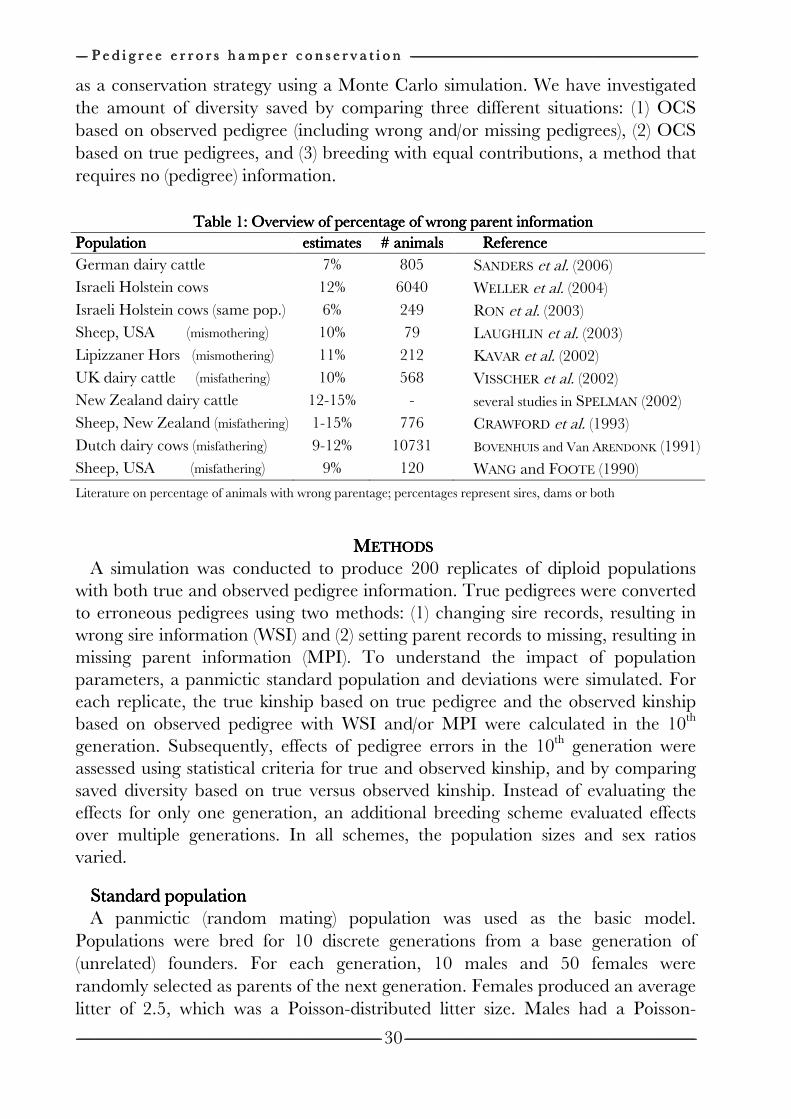
-------------------- P e d i g r e e e r r o r s h a m p e r c o n s e r v a t i o n P e d i g r e e e r r o r s h a m p e r c o n s e r v a t i o n P e d i g r e e e r r o r s h a m p e r c o n s e r v a t i o n P e d i g r e e e r r o r s h a m p e r c o n s e r v a t i o n --------------------------------------------------------------------------------------------------------------------------------------------------------------------------------------------------------------------------------------------------------------------------------------------------------------------------------------------------------------------------------------------------------------------------------------------------------------------------------------------------------------------------------------------------------------------------------------------------------
-------------------------------------------------------------------------------------------------------------------------------------------------------------------------------------------------------------------------------------------------------------------------------------------------------------------------------------------------------------------------------------------------------------------------------------------------------------------------------------------------------------------------------------------------------------------------------------------------------------------------------------------- ----------------------------------------------------------------------------------------------------------------------------------------------------------------------------------------------------------------------------------------------------------------------------------------------------------------------------------------------------------------------------------------------------------------------------------------------------------------------------------------------------------------------------------------------------------------------------------------------------------------
30
as a conservation strategy using a Monte Carlo simulation. We have investigated the amount of diversity saved by comparing three different situations: (1) OCS based on observed pedigree (including wrong and/or missing pedigrees), (2) OCS based on true pedigrees, and (3) breeding with equal contributions, a method that requires no (pedigree) information.
Table 1: Overview of percentage of wrong parent informationTable 1: Overview of percentage of wrong parent informationTable 1: Overview of percentage of wrong parent informationTable 1: Overview of percentage of wrong parent information
PopulationPopulationPopulationPopulation estimatesestimatesestimatesestimates # animals# animals# animals# animals ReferenceReferenceReferenceReference
German dairy cattle 7% 805 SANDERS et al. (2006) Israeli Holstein cows 12% 6040 WELLER et al. (2004) Israeli Holstein cows (same pop.) 6% 249 RON et al. (2003) Sheep, USA (mismothering) 10% 79 LAUGHLIN et al. (2003) Lipizzaner Hors (mismothering) 11% 212 KAVAR et al. (2002) UK dairy cattle (misfathering) 10% 568 VISSCHER et al. (2002) New Zealand dairy cattle 12-15% - several studies in SPELMAN (2002) Sheep, New Zealand (misfathering) 1-15% 776 CRAWFORD et al. (1993) Dutch dairy cows (misfathering) 9-12% 10731 BOVENHUIS and Van ARENDONK (1991) Sheep, USA (misfathering) 9% 120 WANG and FOOTE (1990)
Literature on percentage of animals with wrong parentage; percentages represent sires, dams or both
MMMMETHODSETHODSETHODSETHODS A simulation was conducted to produce 200 replicates of diploid populations
with both true and observed pedigree information. True pedigrees were converted to erroneous pedigrees using two methods: (1) changing sire records, resulting in wrong sire information (WSI) and (2) setting parent records to missing, resulting in missing parent information (MPI). To understand the impact of population parameters, a panmictic standard population and deviations were simulated. For each replicate, the true kinship based on true pedigree and the observed kinship based on observed pedigree with WSI and/or MPI were calculated in the 10th generation. Subsequently, effects of pedigree errors in the 10th generation were assessed using statistical criteria for true and observed kinship, and by comparing saved diversity based on true versus observed kinship. Instead of evaluating the effects for only one generation, an additional breeding scheme evaluated effects over multiple generations. In all schemes, the population sizes and sex ratios varied.
Standard populationStandard populationStandard populationStandard population A panmictic (random mating) population was used as the basic model.
Populations were bred for 10 discrete generations from a base generation of (unrelated) founders. For each generation, 10 males and 50 females were randomly selected as parents of the next generation. Females produced an average litter of 2.5, which was a Poisson-distributed litter size. Males had a Poisson-
------------------------------------------------------------------------------------------------------------------------------------------------------------------------------------------------------------------------------------------------------------------------------------------------------------------------------------------------------------------------------------------------------------------------------------------------------------------------------------------------------------------------------------------------------------------------------------------------------------------------------------------------------------------------------------------------------------------------------------------------------------------------------------------------------------------------------------------------------------------------------------------------------------------------------------------------------------------------------------------------------------------------------------------------------------------------------------------------ C h a p t e r C h a p t e r C h a p t e r C h a p t e r 3333 --------------------
---------------------------------------------------------------------------------------------------------------------------------------------------------------------------------------------------------------------------------------------------------------------------------------------------------------------------------------------------------------------------------------------------------------------------------------------------------------------------------------------------------------------------------------------------------------------------------------------------------------------------------------- --------------------------------------------------------------------------------------------------------------------------------------------------------------------------------------------------------------------------------------------------------------------------------------------------------------------------------------------------------------------------------------------------------------------------------------------------------------------------------------------------------------------------------------------------------------------------------------------------------
31
distributed number of mates (on average 5) and the average number of progeny was 12.5. For each generation, offspring were produced using random mating and both the true and observed pedigrees were recorded. Parameters derived from observed pedigree information are indicated with ‘~~~~’ in this paper. True kinship (ƒ) between individuals was calculated from the true pedigree, and observed kinship ( f~ ) was calculated from the observed pedigree using the tabular method (EMIK and TERRILL, 1949). The 10th generation had a fixed number of 100 individuals (candidate parents).
Erroneous pedigreesErroneous pedigreesErroneous pedigreesErroneous pedigrees Wrong sire information (WSI): For each generation, observed pedigrees were
created from true pedigrees by substituting 0% to 25% of the true fathers by another father taken at random from the same generation as the true father.
Missing parent information (MPI): For each generation, observed pedigrees were created from true pedigrees, by setting, sires, or both parents to missing for 0% to 100% random individuals.
WSI and MPI combined: The combined effect of WSI and MPI was investigated by applying 0% to 100% MPI on the standard population with 10% WSI.
Correction for missing pedigree information Correction for missing pedigree information Correction for missing pedigree information Correction for missing pedigree information Kinship can be corrected for MPI. VANRADEN (1992) stated that unknown
parents should be related to all other parents by twice the mean inbreeding level of the period. Instead of mean inbreeding level, the average mean kinship among parents was used.
AnalysisAnalysisAnalysisAnalysis For each replicate, both true and observed kinships were calculated between all
pairs of individuals from the 10th generation using the tabular method (EMIK and TERRILL, 1949). The effect of WSI and/or MPI was investigated by comparing true and observed kinships using two types of criteria: (1) statistical criteria and (2) a diversity criterion.
Statistical criteria: Three statistical criteria were used for the analysis: (1) the correlation between true and observed kinships (ρ), which measures the proportion of the variance in true kinship explained by observed kinship; (2) the regression coefficient of observed kinship on true kinship (β1), which is a measure for bias in the observed differences in kinship among pairs of individuals; and (3) the regression coefficient of true kinship on observed kinship (β2), which indicates whether observed kinship is an “unbiased” prediction of true kinship. In practice, the latter is important since conservation decisions are based on observed kinship and not on true values (see also Chapter 5). Kinship of individuals with themselves was excluded from all three statistical criteria.
-------------------- P e d i g r e e e r r o r s h a m p e r c o n s e r v a t i o n P e d i g r e e e r r o r s h a m p e r c o n s e r v a t i o n P e d i g r e e e r r o r s h a m p e r c o n s e r v a t i o n P e d i g r e e e r r o r s h a m p e r c o n s e r v a t i o n --------------------------------------------------------------------------------------------------------------------------------------------------------------------------------------------------------------------------------------------------------------------------------------------------------------------------------------------------------------------------------------------------------------------------------------------------------------------------------------------------------------------------------------------------------------------------------------------------------
-------------------------------------------------------------------------------------------------------------------------------------------------------------------------------------------------------------------------------------------------------------------------------------------------------------------------------------------------------------------------------------------------------------------------------------------------------------------------------------------------------------------------------------------------------------------------------------------------------------------------------------------- ----------------------------------------------------------------------------------------------------------------------------------------------------------------------------------------------------------------------------------------------------------------------------------------------------------------------------------------------------------------------------------------------------------------------------------------------------------------------------------------------------------------------------------------------------------------------------------------------------------------
32
Diversity measures: Though statistical criteria are informative, they do not directly reveal the amount of conserved genetic diversity when using observed pedigrees in practice. In addition, we applied a diversity criterion, DS, which evaluates the Diversity Saved when optimal contributions are based on observed pedigrees. DS was calculated from three underlying diversity measures, which are expressed on the scale of founder genome equivalents (FGE) (CABALLERO and TORO, 2000). FGEs are the number of equally contributing founders with no random loss of founder alleles in descendants that would be expected to produce the same genetic diversity (or kinship) as the population under study (LACY, 1989; CABALLERO and TORO, 2000). This scale is a natural number and easier to interpret than probabilities or percentages (HOFFRAGE et al., 2000). The three underlying diversity measures were (1) NEC, genetic diversity conserved when equal contributions were applied; (2) NOC , genetic diversity conserved when OCS were applied based on true kinship; and (3)
OC�~ , the genetic diversity conserved
when OCS were applied based on observed kinship (hence the ‘~~~~’). The three diversity measures NEC, NOC , and
OC�~ were based on a weighted
average mean kinship among candidate parents (MEUWISSEN, 1997). The diversity measures (dm) were calculated using the following Equation:
Fcc'*�dm
2
1= ,, ((11))
where FFFF is a matrix of true kinships among all individuals, including kinship of individuals with themselves, and cccc is a column vector of proportional contributions of candidate parents to future generation (which were always 100 animals in the 10th generation), so that sum of elements of cccc equals one (EMIK and TERRILL, 1949). By varying the contributions of individuals (cccc), average mean kinship among candidates, and thus the average mean kinship in the future generations, can be increased or decreased.
NEC was calculated by substituting cccc in Equation 1 with ccccEC, which is a vector of equal contributions per candidate parent, so that the sum of elements of ccccEC equals one. NEC is simply the average mean kinship of the current population, expressed on the scale of FGE.
NOC was calculated by substituting cccc in Equation 1 with ccccOC, which is an optimum contribution vector that minimizes c’Fcc’Fcc’Fcc’Fc, and therefore maximizes diversity.
OCc is given by:
1F1'
1Fc
1
1
−
−
=OC,, ((22))
where 1111 is a column vector of ones. When negative contributions were obtained, the most negative contribution was set to zero and vector
OCc was recalculated until all contributions were non-negative. This method does not necessarily find the true optimal solution. True optimum was always found, however, when contributions were not fixed a priori (PONG-WONG and WOOLLIAMS, 2007). NOC
------------------------------------------------------------------------------------------------------------------------------------------------------------------------------------------------------------------------------------------------------------------------------------------------------------------------------------------------------------------------------------------------------------------------------------------------------------------------------------------------------------------------------------------------------------------------------------------------------------------------------------------------------------------------------------------------------------------------------------------------------------------------------------------------------------------------------------------------------------------------------------------------------------------------------------------------------------------------------------------------------------------------------------------------------------------------------------------------ C h a p t e r C h a p t e r C h a p t e r C h a p t e r 3333 --------------------
---------------------------------------------------------------------------------------------------------------------------------------------------------------------------------------------------------------------------------------------------------------------------------------------------------------------------------------------------------------------------------------------------------------------------------------------------------------------------------------------------------------------------------------------------------------------------------------------------------------------------------------- --------------------------------------------------------------------------------------------------------------------------------------------------------------------------------------------------------------------------------------------------------------------------------------------------------------------------------------------------------------------------------------------------------------------------------------------------------------------------------------------------------------------------------------------------------------------------------------------------------
33
measures the diversity that could be obtained in future generations (assuming overlap) and a practical example is the selection of animals for a gene bank to reconstruct a future population.
OC�~ was calculated by substituting cccc in Equation 1 with the observed optimum
contribution vector (OCc~ ).
OCc~ was calculated by substituting FFFF in Equation 2 by the
matrix of observed kinship ( ). OC�~ measures the obtained diversity when OCS is
applied on observed pedigrees. The diversity criterion represents the fraction Diversity Saved (DS) by applying
optimal contributions based on observed pedigree; this was calculated as follows:
ECOC
ECOC
��
��DS
−
−=
~
.. ((33))
DS evaluates the Diversity Saved when optimal contributions were based on observed pedigrees;
ECOC �� −~ , as a fraction of the full amount of diversity that
could have been saved with optimal contributions based on true pedigree data;
ECOC �� − . Equal contributions were used as a base of comparison, as this would be the logical selection method if no information on kinship is available.
Note that in practice not all the individuals can be parent, even when desired, which causes genetic drift. This could cause a setback in the genetic diversity gained for both equal contribution- as well as optimal contribution-schemes.
The ‘observed NOC’ (OC�~~ ) was calculated by substituting cccc and FFFF in Equation 1
with OCc~ and F~ . Breeders only have observed pedigrees. Therefore, the true
genetic diversity obtained due to optimal contributions (OC�~~ ) is not known to
breeders. Hence, OC�~~ is the genetic diversity that breeders predict to obtain, based
on the observed pedigrees.
Optimal contribution selection scheme for multiple generations Optimal contribution selection scheme for multiple generations Optimal contribution selection scheme for multiple generations Optimal contribution selection scheme for multiple generations To analyze the effect of WSI and MPI on genetic diversity over multiple
generations, OCS was applied as a breeding scheme. The first five generations were randomly bred like the standard population. The following five generations were bred using OCS based on observed pedigrees. Each sex contributed half the genes to the next generation. OCS were calculated including this constraint using SONESSON and MEUWISSEN (2001):
1Q'FQFQc111 }])
~)[(
~{(~ −−−=OC
,, ((44))
where OCc~ is a vector of proportional contributions of (n) selection candidates to
the next generation, so that contributions of males within OCc~ equals ½ and
contributions of females within OCc~ equals ½, F~ is a matrix of kinship based on
observed pedigrees, 1111 is a column vector of ones, and QQQQ is a (2 × n) design matrix indicating sex of the selection candidates. When negative contributions were obtained, the most negative contribution was set to zero and
OCc~ was recalculated
until all contributions were non-negative. Next, these continuous contributions per candidate were converted into a desired number of offspring per candidate. Each
F~
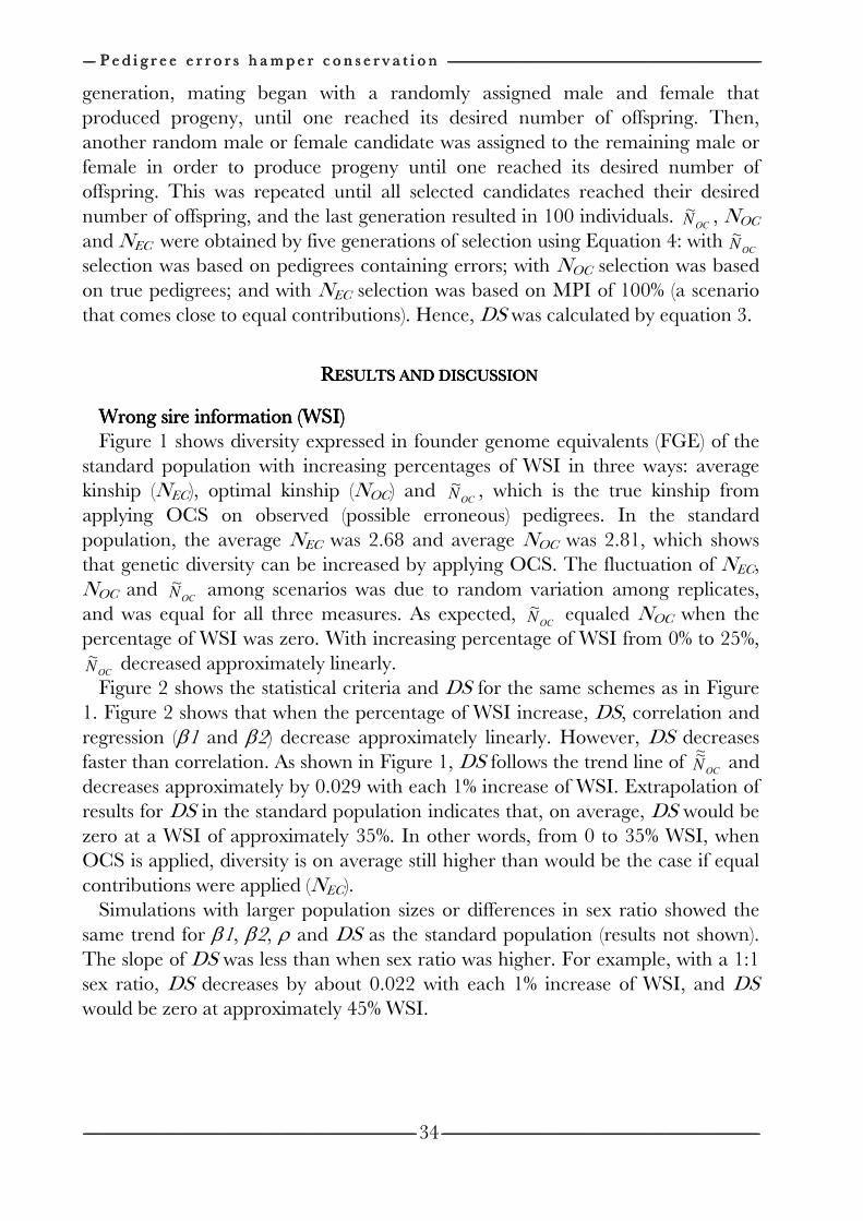
-------------------- P e d i g r e e e r r o r s h a m p e r c o n s e r v a t i o n P e d i g r e e e r r o r s h a m p e r c o n s e r v a t i o n P e d i g r e e e r r o r s h a m p e r c o n s e r v a t i o n P e d i g r e e e r r o r s h a m p e r c o n s e r v a t i o n --------------------------------------------------------------------------------------------------------------------------------------------------------------------------------------------------------------------------------------------------------------------------------------------------------------------------------------------------------------------------------------------------------------------------------------------------------------------------------------------------------------------------------------------------------------------------------------------------------
-------------------------------------------------------------------------------------------------------------------------------------------------------------------------------------------------------------------------------------------------------------------------------------------------------------------------------------------------------------------------------------------------------------------------------------------------------------------------------------------------------------------------------------------------------------------------------------------------------------------------------------------- ----------------------------------------------------------------------------------------------------------------------------------------------------------------------------------------------------------------------------------------------------------------------------------------------------------------------------------------------------------------------------------------------------------------------------------------------------------------------------------------------------------------------------------------------------------------------------------------------------------------
34
generation, mating began with a randomly assigned male and female that produced progeny, until one reached its desired number of offspring. Then, another random male or female candidate was assigned to the remaining male or female in order to produce progeny until one reached its desired number of offspring. This was repeated until all selected candidates reached their desired number of offspring, and the last generation resulted in 100 individuals.
OC�~ , NOC
and NEC were obtained by five generations of selection using Equation 4: with OC�~
selection was based on pedigrees containing errors; with NOC selection was based on true pedigrees; and with NEC selection was based on MPI of 100% (a scenario that comes close to equal contributions). Hence, DS was calculated by equation 3.
RRRRESULTS AND DISCUSSIOESULTS AND DISCUSSIOESULTS AND DISCUSSIOESULTS AND DISCUSSIONNNN
Wrong sire information (WSI)Wrong sire information (WSI)Wrong sire information (WSI)Wrong sire information (WSI) Figure 1 shows diversity expressed in founder genome equivalents (FGE) of the
standard population with increasing percentages of WSI in three ways: average kinship (NEC), optimal kinship (NOC) and
OC�~ , which is the true kinship from
applying OCS on observed (possible erroneous) pedigrees. In the standard population, the average NEC was 2.68 and average NOC was 2.81, which shows that genetic diversity can be increased by applying OCS. The fluctuation of NEC, NOC and
OC�~ among scenarios was due to random variation among replicates,
and was equal for all three measures. As expected, OC�~ equaled NOC when the
percentage of WSI was zero. With increasing percentage of WSI from 0% to 25%,
OC�~ decreased approximately linearly.
Figure 2 shows the statistical criteria and DS for the same schemes as in Figure 1. Figure 2 shows that when the percentage of WSI increase, DS, correlation and regression (β1 and β2) decrease approximately linearly. However, DS decreases faster than correlation. As shown in Figure 1, DS follows the trend line of
OC�~~ and
decreases approximately by 0.029 with each 1% increase of WSI. Extrapolation of results for DS in the standard population indicates that, on average, DS would be zero at a WSI of approximately 35%. In other words, from 0 to 35% WSI, when OCS is applied, diversity is on average still higher than would be the case if equal contributions were applied (NEC).
Simulations with larger population sizes or differences in sex ratio showed the same trend for β1, β2, ρ and DS as the standard population (results not shown). The slope of DS was less than when sex ratio was higher. For example, with a 1:1 sex ratio, DS decreases by about 0.022 with each 1% increase of WSI, and DS would be zero at approximately 45% WSI.
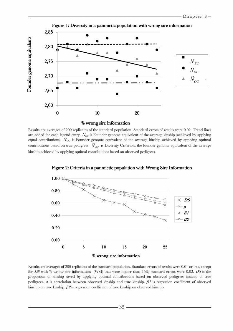
------------------------------------------------------------------------------------------------------------------------------------------------------------------------------------------------------------------------------------------------------------------------------------------------------------------------------------------------------------------------------------------------------------------------------------------------------------------------------------------------------------------------------------------------------------------------------------------------------------------------------------------------------------------------------------------------------------------------------------------------------------------------------------------------------------------------------------------------------------------------------------------------------------------------------------------------------------------------------------------------------------------------------------------------------------------------------------------------ C h a p t e r C h a p t e r C h a p t e r C h a p t e r 3333 --------------------
---------------------------------------------------------------------------------------------------------------------------------------------------------------------------------------------------------------------------------------------------------------------------------------------------------------------------------------------------------------------------------------------------------------------------------------------------------------------------------------------------------------------------------------------------------------------------------------------------------------------------------------- --------------------------------------------------------------------------------------------------------------------------------------------------------------------------------------------------------------------------------------------------------------------------------------------------------------------------------------------------------------------------------------------------------------------------------------------------------------------------------------------------------------------------------------------------------------------------------------------------------
35
2,602,602,602,60
2,652,652,652,65
2,702,702,702,70
2,752,752,752,75
2,802,802,802,80
2,852,852,852,85
0000 10101010 20202020
Foun
der
geno
me
equi
vale
nts
Foun
der
geno
me
equi
vale
nts
Foun
der
geno
me
equi
vale
nts
Foun
der
geno
me
equi
vale
nts
% wrong sire information% wrong sire information% wrong sire information% wrong sire information
....
EC�
OC�
OC�~
Figure 1: Diversity in a panmictic population with wrong sire informationFigure 1: Diversity in a panmictic population with wrong sire informationFigure 1: Diversity in a panmictic population with wrong sire informationFigure 1: Diversity in a panmictic population with wrong sire information Results are averages of 200 replicates of the standard population. Standard errors of results were 0.02. Trend lines are added for each legend entry. NEC is Founder genome equivalent of the average kinship (achieved by applying equal contributions). NOC is Founder genome equivalent of the average kinship achieved by applying optimal
contributions based on true pedigrees. OC�~ is Diversity Criterion, the founder genome equivalent of the average
kinship achieved by applying optimal contributions based on observed pedigrees.
Figure 2: Criteria in a panmictic population with Figure 2: Criteria in a panmictic population with Figure 2: Criteria in a panmictic population with Figure 2: Criteria in a panmictic population with Wrong Sire InformationWrong Sire InformationWrong Sire InformationWrong Sire Information
Results are averages of 200 replicates of the standard population. Standard errors of results were 0.01 or less, except for DS with % wrong sire information (WSI) that were higher than 15%; standard errors were 0.02. DS is the proportion of kinship saved by applying optimal contributions based on observed pedigrees instead of true pedigrees. ρ is correlation between observed kinship and true kinship. β1 is regression coefficient of observed kinship on true kinship. β2 is regression coefficient of true kinship on observed kinship.
0.000.000.000.00
0.200.200.200.20
0.400.400.400.40
0.600.600.600.60
0.800.800.800.80
1.001.001.001.00
0000 5555 10101010 15151515 20202020 25252525
% wrong sire information% wrong sire information% wrong sire information% wrong sire information
DSDSDSDS
ρ
ß1ß1ß1ß1
ß2ß2ß2ß2
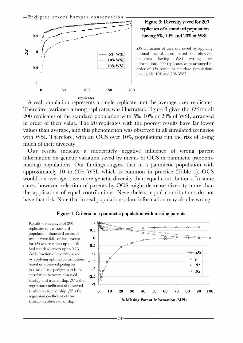
-------------------- P e d i g r e e e r r o r s h a m p e r c o n s e r v a t i o n P e d i g r e e e r r o r s h a m p e r c o n s e r v a t i o n P e d i g r e e e r r o r s h a m p e r c o n s e r v a t i o n P e d i g r e e e r r o r s h a m p e r c o n s e r v a t i o n --------------------------------------------------------------------------------------------------------------------------------------------------------------------------------------------------------------------------------------------------------------------------------------------------------------------------------------------------------------------------------------------------------------------------------------------------------------------------------------------------------------------------------------------------------------------------------------------------------
-------------------------------------------------------------------------------------------------------------------------------------------------------------------------------------------------------------------------------------------------------------------------------------------------------------------------------------------------------------------------------------------------------------------------------------------------------------------------------------------------------------------------------------------------------------------------------------------------------------------------------------------- ----------------------------------------------------------------------------------------------------------------------------------------------------------------------------------------------------------------------------------------------------------------------------------------------------------------------------------------------------------------------------------------------------------------------------------------------------------------------------------------------------------------------------------------------------------------------------------------------------------------
36
-1-1-1-1
-0.5-0.5-0.5-0.5
0000
0.50.50.50.5
1111
0000 50505050 100100100100 150150150150 200200200200
replicatesreplicatesreplicatesreplicates
DS
DS
DS
DS
5% WSI 5% WSI 5% WSI 5% WSI
10% WSI10% WSI10% WSI10% WSI
20% WSI20% WSI20% WSI20% WSI
-3-3-3-3
-2.5-2.5-2.5-2.5
-2-2-2-2
-1.5-1.5-1.5-1.5
-1-1-1-1
-0.5-0.5-0.5-0.5
0000
0.50.50.50.5
1111
0000 10101010 20202020 30303030 40404040 50505050 60606060 70707070 80808080 90909090 100100100100
% Missing Parent Information (MPI)% Missing Parent Information (MPI)% Missing Parent Information (MPI)% Missing Parent Information (MPI)
DSDSDSDS
ρ
ß1ß1ß1ß1
ß2ß2ß2ß2
A real population represents a single replicate, not the average over replicates.
Therefore, variance among replicates was illustrated. Figure 3 gives the DS for all 200 replicates of the standard population with 5%, 10% or 20% of WSI, arranged in order of their value. The 20 replicates with the poorest results have far lower values than average, and this phenomenon was observed in all simulated scenarios with WSI. Therefore, with an OCS over 10%, populations run the risk of losing much of their diversity
Our results indicate a moderately negative influence of wrong parent information on genetic variation saved by means of OCS in panmictic (random-mating) populations. Our findings suggest that in a panmictic population with approximately 10 to 20% WSI, which is common in practice (Table 1), OCS would, on average, save more genetic diversity than equal contributions. In some cases, however, selection of parents by OCS might decrease diversity more than the application of equal contributions. Nevertheless, equal contributions do not have that risk. Note that in real populations, dam information may also be wrong.
Figure 4: Figure 4: Figure 4: Figure 4: CCCCriteria in a panmictic population with missing parentsriteria in a panmictic population with missing parentsriteria in a panmictic population with missing parentsriteria in a panmictic population with missing parents
Figure 3: Diversity saved for 200 Figure 3: Diversity saved for 200 Figure 3: Diversity saved for 200 Figure 3: Diversity saved for 200
replicates of a standard population replicates of a standard population replicates of a standard population replicates of a standard population
having 5%, 10% and 20% of WSIhaving 5%, 10% and 20% of WSIhaving 5%, 10% and 20% of WSIhaving 5%, 10% and 20% of WSI
DS is fraction of diversity saved by applying optimal contributions based on observed pedigrees having WSI (wrong sire information). 200 replicates were arranged in order of DS result for standard populations having 5%, 10% and 20% WSI.
Results are averages of 200 replicates of the standard population. Standard errors of results were 0.01 or less, except for DS where values up to 40% had standard errors up to 0.13. DS is fraction of diversity saved by applying optimal contributions based on observed pedigrees instead of true pedigrees. ρ is the correlation between observed kinship and true kinship. β1 is the regression coefficient of observed kinship on true kinship. β2 is the regression coefficient of true kinship on observed kinship.
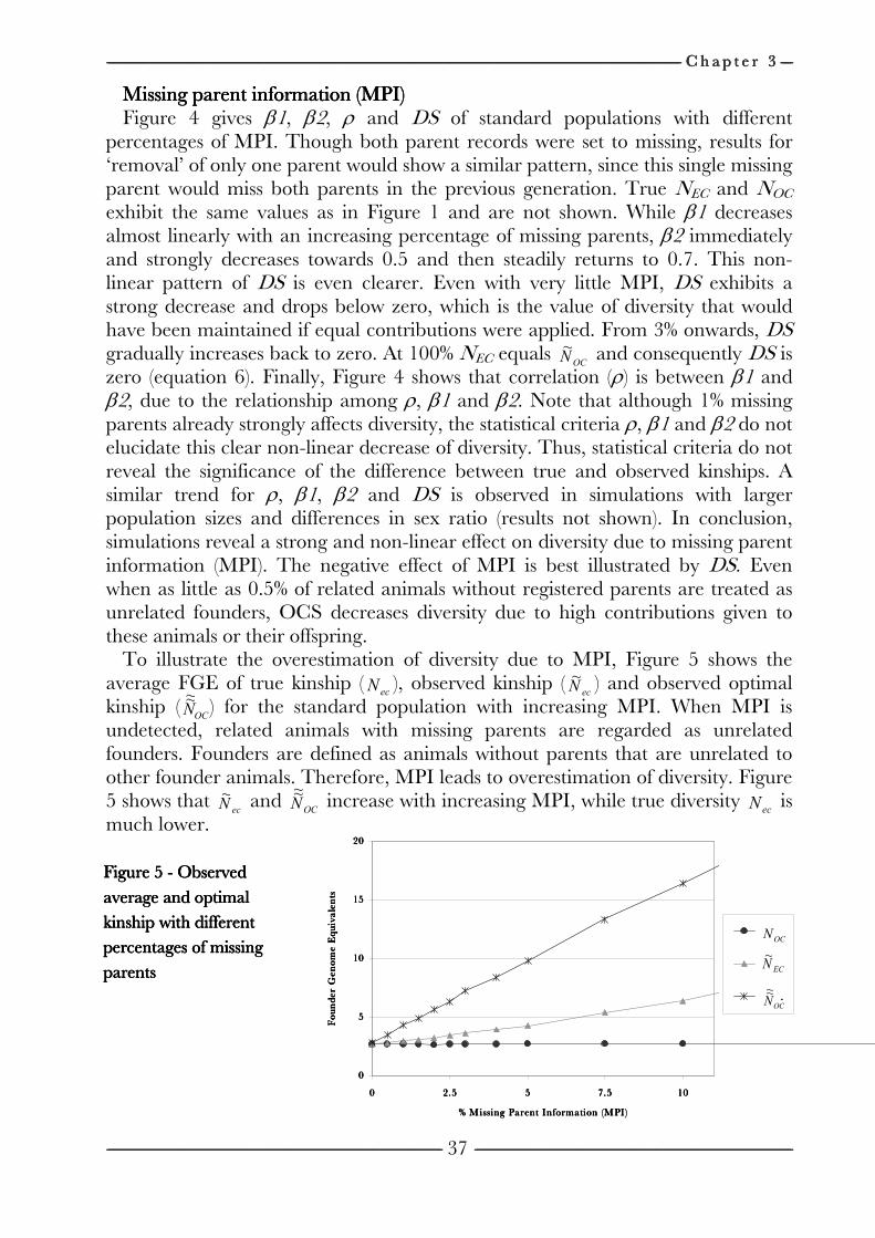
------------------------------------------------------------------------------------------------------------------------------------------------------------------------------------------------------------------------------------------------------------------------------------------------------------------------------------------------------------------------------------------------------------------------------------------------------------------------------------------------------------------------------------------------------------------------------------------------------------------------------------------------------------------------------------------------------------------------------------------------------------------------------------------------------------------------------------------------------------------------------------------------------------------------------------------------------------------------------------------------------------------------------------------------------------------------------------------------ C h a p t e r C h a p t e r C h a p t e r C h a p t e r 3333 --------------------
---------------------------------------------------------------------------------------------------------------------------------------------------------------------------------------------------------------------------------------------------------------------------------------------------------------------------------------------------------------------------------------------------------------------------------------------------------------------------------------------------------------------------------------------------------------------------------------------------------------------------------------- --------------------------------------------------------------------------------------------------------------------------------------------------------------------------------------------------------------------------------------------------------------------------------------------------------------------------------------------------------------------------------------------------------------------------------------------------------------------------------------------------------------------------------------------------------------------------------------------------------
37
0000
5555
10101010
15151515
20202020
0000 2.52.52.52.5 5555 7.57.57.57.5 10101010
% Missing Parent Information (MPI)% Missing Parent Information (MPI)% Missing Parent Information (MPI)% Missing Parent Information (MPI)
Fo
un
der
Gen
om
e E
qu
iva
len
tsF
ou
nd
er G
eno
me
Eq
uiv
ale
nts
Fo
un
der
Gen
om
e E
qu
iva
len
tsF
ou
nd
er G
eno
me
Eq
uiv
ale
nts
. . . .
EC�~
OC�~~
OC�
Missing parent information (MPI)Missing parent information (MPI)Missing parent information (MPI)Missing parent information (MPI) Figure 4 gives β1, β2, ρ and DS of standard populations with different
percentages of MPI. Though both parent records were set to missing, results for ‘removal’ of only one parent would show a similar pattern, since this single missing parent would miss both parents in the previous generation. True NEC and NOC exhibit the same values as in Figure 1 and are not shown. While β1 decreases almost linearly with an increasing percentage of missing parents, β2 immediately and strongly decreases towards 0.5 and then steadily returns to 0.7. This non-linear pattern of DS is even clearer. Even with very little MPI, DS exhibits a strong decrease and drops below zero, which is the value of diversity that would have been maintained if equal contributions were applied. From 3% onwards, DS gradually increases back to zero. At 100% NEC equals
OC�~ and consequently DS is
zero (equation 6). Finally, Figure 4 shows that correlation (ρ) is between β1 and β2, due to the relationship among ρ, β1 and β2. Note that although 1% missing parents already strongly affects diversity, the statistical criteria ρ, β1 and β2 do not elucidate this clear non-linear decrease of diversity. Thus, statistical criteria do not reveal the significance of the difference between true and observed kinships. A similar trend for ρ, β1, β2 and DS is observed in simulations with larger population sizes and differences in sex ratio (results not shown). In conclusion, simulations reveal a strong and non-linear effect on diversity due to missing parent information (MPI). The negative effect of MPI is best illustrated by DS. Even when as little as 0.5% of related animals without registered parents are treated as unrelated founders, OCS decreases diversity due to high contributions given to these animals or their offspring.
To illustrate the overestimation of diversity due to MPI, Figure 5 shows the average FGE of true kinship (
ec� ), observed kinship (ec�~ ) and observed optimal
kinship (OC�~~ ) for the standard population with increasing MPI. When MPI is
undetected, related animals with missing parents are regarded as unrelated founders. Founders are defined as animals without parents that are unrelated to other founder animals. Therefore, MPI leads to overestimation of diversity. Figure 5 shows that
ec�~ and
OC�~~ increase with increasing MPI, while true diversity
ec� is much lower.
Figure 5 Figure 5 Figure 5 Figure 5 ---- Observed Observed Observed Observed
average and optimal average and optimal average and optimal average and optimal
kinship with different kinship with different kinship with different kinship with different
percentages of missing percentages of missing percentages of missing percentages of missing
parentsparentsparentsparents
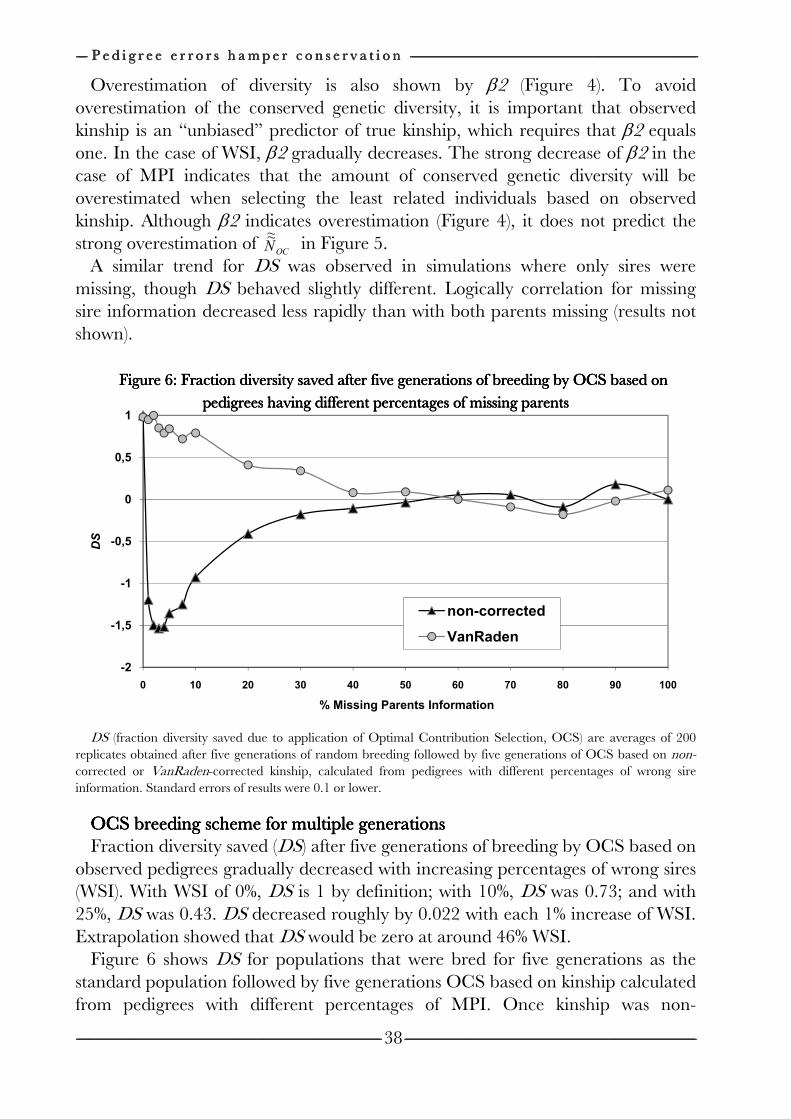
-------------------- P e d i g r e e e r r o r s h a m p e r c o n s e r v a t i o n P e d i g r e e e r r o r s h a m p e r c o n s e r v a t i o n P e d i g r e e e r r o r s h a m p e r c o n s e r v a t i o n P e d i g r e e e r r o r s h a m p e r c o n s e r v a t i o n --------------------------------------------------------------------------------------------------------------------------------------------------------------------------------------------------------------------------------------------------------------------------------------------------------------------------------------------------------------------------------------------------------------------------------------------------------------------------------------------------------------------------------------------------------------------------------------------------------
-------------------------------------------------------------------------------------------------------------------------------------------------------------------------------------------------------------------------------------------------------------------------------------------------------------------------------------------------------------------------------------------------------------------------------------------------------------------------------------------------------------------------------------------------------------------------------------------------------------------------------------------- ----------------------------------------------------------------------------------------------------------------------------------------------------------------------------------------------------------------------------------------------------------------------------------------------------------------------------------------------------------------------------------------------------------------------------------------------------------------------------------------------------------------------------------------------------------------------------------------------------------------
38
-2
-1,5
-1
-0,5
0
0,5
1
0 10 20 30 40 50 60 70 80 90 100
DS
% Missing Parents Information
non-corrected
VanRaden
Overestimation of diversity is also shown by β2 (Figure 4). To avoid overestimation of the conserved genetic diversity, it is important that observed kinship is an “unbiased” predictor of true kinship, which requires that β2 equals one. In the case of WSI, β2 gradually decreases. The strong decrease of β2 in the case of MPI indicates that the amount of conserved genetic diversity will be overestimated when selecting the least related individuals based on observed kinship. Although β2 indicates overestimation (Figure 4), it does not predict the strong overestimation of
OC�~~ in Figure 5.
A similar trend for DS was observed in simulations where only sires were missing, though DS behaved slightly different. Logically correlation for missing sire information decreased less rapidly than with both parents missing (results not shown).
Figure 6: Fraction diversity saved after five generations of breeding by OCS based on Figure 6: Fraction diversity saved after five generations of breeding by OCS based on Figure 6: Fraction diversity saved after five generations of breeding by OCS based on Figure 6: Fraction diversity saved after five generations of breeding by OCS based on
pedigrees havpedigrees havpedigrees havpedigrees having different percentages of missing parentsing different percentages of missing parentsing different percentages of missing parentsing different percentages of missing parents
DS (fraction diversity saved due to application of Optimal Contribution Selection, OCS) are averages of 200
replicates obtained after five generations of random breeding followed by five generations of OCS based on non-corrected or VanRaden-corrected kinship, calculated from pedigrees with different percentages of wrong sire information. Standard errors of results were 0.1 or lower.
OCS breeding scheme for multiple generationsOCS breeding scheme for multiple generationsOCS breeding scheme for multiple generationsOCS breeding scheme for multiple generations Fraction diversity saved (DS) after five generations of breeding by OCS based on
observed pedigrees gradually decreased with increasing percentages of wrong sires (WSI). With WSI of 0%, DS is 1 by definition; with 10%, DS was 0.73; and with 25%, DS was 0.43. DS decreased roughly by 0.022 with each 1% increase of WSI. Extrapolation showed that DS would be zero at around 46% WSI.
Figure 6 shows DS for populations that were bred for five generations as the standard population followed by five generations OCS based on kinship calculated from pedigrees with different percentages of MPI. Once kinship was non-
------------------------------------------------------------------------------------------------------------------------------------------------------------------------------------------------------------------------------------------------------------------------------------------------------------------------------------------------------------------------------------------------------------------------------------------------------------------------------------------------------------------------------------------------------------------------------------------------------------------------------------------------------------------------------------------------------------------------------------------------------------------------------------------------------------------------------------------------------------------------------------------------------------------------------------------------------------------------------------------------------------------------------------------------------------------------------------------------ C h a p t e r C h a p t e r C h a p t e r C h a p t e r 3333 --------------------
---------------------------------------------------------------------------------------------------------------------------------------------------------------------------------------------------------------------------------------------------------------------------------------------------------------------------------------------------------------------------------------------------------------------------------------------------------------------------------------------------------------------------------------------------------------------------------------------------------------------------------------- --------------------------------------------------------------------------------------------------------------------------------------------------------------------------------------------------------------------------------------------------------------------------------------------------------------------------------------------------------------------------------------------------------------------------------------------------------------------------------------------------------------------------------------------------------------------------------------------------------
39
corrected as in Figure 4, and once kinship was corrected for missing pedigree information by VANRADEN (1992). For non-corrected OCS, DS decreases strongly at levels as low as 0.5% MPI, and then drops below zero. From 5% missing parents onwards, DS increases again towards zero. For VanRaden-corrected OCS, DS starts at 1 and gradually drops to zero until 50% MPI. From 50% MPI and upward, on average no apparent difference is observed between equal contributions and OCS based on non- or VanRaden corrected kinship. Figure 6 shows again that OCS based non-corrected kinship calculated from pedigrees with MSI can only decrease diversity. Comparing Figure 6 with results with Figure 2, which shows results for a single generation, the decrease is not as strong as expected if all five generations were affected by MPI as strongly as a single generation. The reason for this is that the error did not accumulate each generation after it is ‘incorporated’ by OCS. Therefore relative loss due to pedigree errors mainly occurred in the first generation that started OCS.
This research investigated a panmictic population, assuming control over a population. In practice, species or populations differ in population structure due to aspects like unequal sex ratio and/or limited number of progeny per female, etc. Conservationists have to consider these constraints. With unequal sex-ratio for example, equal contributions cannot be applied and instead optimal management of mate selection across multiple generations yield lowest rates of increase of kinship (FERNANDEZ et al., 2003; SÁNCHEZ et al., 2003).
CCCCONCLUSIONSONCLUSIONSONCLUSIONSONCLUSIONS The results imply that using only pedigree information in conservation warrants
caution. On average, the genetic diversity saved by optimal contributions is less with low percentages of WSI. If WSI is over 35%, on average, optimal contributions preserve less genetic diversity than equal contributions. The impact of WSI on genetic diversity for a single population, however, might deviate from this average (Figure 3). In addition, when pedigrees are known to contain more than approximately 15% wrong parent information (misidentified fathers plus mothers) in a panmictic population, conservationist should consider alternative breeding methods, because expected gain is relatively low compared to alternatives like optimal management of mate selection across multiple generations. Populations in need of conservation, however, often deviate from a panmictic population. Furthermore, the type of error expected should also be taken into consideration. This research investigated the worst type of WSI. In practice, misidentified sires are sometimes related to the true sire, for example with natural mating within herds. We also found that DS decreased slower due to VanRaden-corrected MPI (Figure 6) than due to WSI (Figure 4). In conclusion, wrong parent information above 15% might be acceptable in practice, depending on the type of error and the population structure. Traditionally, MPI is bypassed
-------------------- P e d i g r e e e r r o r s h a m p e r c o n s e r v a t i o n P e d i g r e e e r r o r s h a m p e r c o n s e r v a t i o n P e d i g r e e e r r o r s h a m p e r c o n s e r v a t i o n P e d i g r e e e r r o r s h a m p e r c o n s e r v a t i o n --------------------------------------------------------------------------------------------------------------------------------------------------------------------------------------------------------------------------------------------------------------------------------------------------------------------------------------------------------------------------------------------------------------------------------------------------------------------------------------------------------------------------------------------------------------------------------------------------------
-------------------------------------------------------------------------------------------------------------------------------------------------------------------------------------------------------------------------------------------------------------------------------------------------------------------------------------------------------------------------------------------------------------------------------------------------------------------------------------------------------------------------------------------------------------------------------------------------------------------------------------------- ----------------------------------------------------------------------------------------------------------------------------------------------------------------------------------------------------------------------------------------------------------------------------------------------------------------------------------------------------------------------------------------------------------------------------------------------------------------------------------------------------------------------------------------------------------------------------------------------------------------
40
by the assumption that animals with unknown parents are founders (BALLOU and LACY, 1995), resulting in an overestimation of the available genetic diversity. Optimal contributions are extremely sensitive to differences in kinship between candidates. Small differences in pedigree can make the difference between significant or zero contribution for an individual animal. Animals with gaps in their pedigree will be considered unrelated and therefore be given high contributions. In this situation, equal contributions to each candidate parent would maintain diversity. Therefore, optimal contributions based on pedigrees with MPI can perform less well than equal contributions.
Overall this indicates that low percentage of MPI should always be corrected prior to the application of OCS. Even a simple correction of MPI by randomly assigned parents would increase diversity, which would leave breeders with wrong parent information. However, to correct for gaps in pedigrees, more sophisticated solutions have been presented. BALLOU and LACY (1995) have proposed the calculation of kinship based only on the portion of the genome that descends from true founder animals, excluding the proportion due to animals with unknown parents. VANRADEN (1992) corrected gaps in pedigrees by assuming that unknown parents are related to all other parents by twice the average inbreeding level of that period. VanRaden is occasionally applied to calculate kinship (COLE, 2007). Compared to VanRaden, the Ballou and Lacy-correction creates more variance among kinship values, which has a possible negative impact on OCS. Therefore, the VanRaden was applied to correct for MPI in this research.
We recommend two policies for conservation. First, measures that avoid errors in pedigree are encouraged. One obvious measure is to sample animal tissue, since DNA can be used both for parentage analysis and kinship estimation (BALLOU, 1997). Second, pedigree-registration, like herd-books, should include information on the status of animals without parent records: whether they are (1) founders (wild-caught or otherwise known to be unrelated) or (2) related and descending from founders. Within kinship calculation, the latter should always be corrected, for example by using the VanRaden or a similar algorithm.
AAAACKNOWLEDGEMENTSCKNOWLEDGEMENTSCKNOWLEDGEMENTSCKNOWLEDGEMENTS We thank Sipke Joost Hiemstra, Jack Windig and Johan van Arendonk for their
thorough comments on previous versions and two anonymous referees for comments and suggestions. This work was financed by the Ministry of Agriculture, Nature and Food Quality through the Centre for Genetic Resources, the Netherlands (CGN).
----------------------------------------------------------------------------------------------------------------------------------------------------------------------------------------------------------------------------------------------------------------------------------------------------------------------------------------------------------------------------------------------------------------------------------------------------------------------------------------------------------------------------------------------------------------------------------------------------------------------------------------------------------------------------------------------------------------------------------------------------------------------------------------------------------------------------------------------------------------------------------------------------------------------------------------------------------------------------------------------------------------------------------------------------------------------------------------------------------------------------------------------------------------------------------------------------------------------------------------------------------------------------------------------------------------
-------------------------------------------------------------------------------------------------------------------------------------------------------------------------------------------------------------------------------------------------------------------------------------------------------------------------------------------------------------------------------------------------------------------------------------------------------------------------------------------------------------------------------------------------------------------------------------------------------------------------------------------- ----------------------------------------------------------------------------------------------------------------------------------------------------------------------------------------------------------------------------------------------------------------------------------------------------------------------------------------------------------------------------------------------------------------------------------------------------------------------------------------------------------------------------------------------------------------------------------------------------------------
41
Correction of kinship for unknown parents Correction of kinship for unknown parents Correction of kinship for unknown parents Correction of kinship for unknown parents
with a focus on their use in conservation programswith a focus on their use in conservation programswith a focus on their use in conservation programswith a focus on their use in conservation programs
C h a p t e r C h a p t e r C h a p t e r C h a p t e r 4444
Pieter A. Oliehoek
SANDERS et al. (2006) WELLER et al. (2004) RON et al. (2003) LAUGHLIN et al.
-------------------- C o r r e c t i o n f o r u n k n o w n p a r e n t s C o r r e c t i o n f o r u n k n o w n p a r e n t s C o r r e c t i o n f o r u n k n o w n p a r e n t s C o r r e c t i o n f o r u n k n o w n p a r e n t s ----------------------------------------------------------------------------------------------------------------------------------------------------------------------------------------------------------------------------------------------------------------------------------------------------------------------------------------------------------------------------------------------------------------------------------------------------------------------------------------------------------------------------------------------------------------------------------------------------------------------------------------------------------------------------------------
-------------------------------------------------------------------------------------------------------------------------------------------------------------------------------------------------------------------------------------------------------------------------------------------------------------------------------------------------------------------------------------------------------------------------------------------------------------------------------------------------------------------------------------------------------------------------------------------------------------------------------------------- ----------------------------------------------------------------------------------------------------------------------------------------------------------------------------------------------------------------------------------------------------------------------------------------------------------------------------------------------------------------------------------------------------------------------------------------------------------------------------------------------------------------------------------------------------------------------------------------------------------------
42
AAAABSTRACTBSTRACTBSTRACTBSTRACT Long-term survival of captive populations depends on captive breeding
management that maintain genetic diversity (GD), especially when the parental wild populations no longer serve as a source of population replacements. Hence, GD management in captive populations is important. Kinship plays a central role in management and breeding decisions. Gaps in pedigrees can strongly influence calculation of kinship. We compared ten methods to correct for gaps in pedigrees. Subsequently, these methods were used to evaluate loss and possible regain of GD using optimal contributions. Three pedigreed zoo populations, which had gaps in the pedigree, served as template for simulating possible true pedigrees.
Correction methods that exclude parts of genomes descending from unknown parents saved less GD, and should only be considered to minimize undesirable introgression, while maximizing GD. For other methods, three factors improved correction of kinship: (1) correct by using kinship instead of inbreeding; (2) taking averages of candidate parents instead of random assignment of one candidate parent for each unknown parent; and (3) identify probable parents of animals with unknown parents and a high contribution to the current population. This research shows that all three studied captive populations could double their GD with optimal contributions when kinship was corrected by averaging kinship of candidate parents.
------------------------------------------------------------------------------------------------------------------------------------------------------------------------------------------------------------------------------------------------------------------------------------------------------------------------------------------------------------------------------------------------------------------------------------------------------------------------------------------------------------------------------------------------------------------------------------------------------------------------------------------------------------------------------------------------------------------------------------------------------------------------------------------------------------------------------------------------------------------------------------------------------------------------------------------------------------------------------------------------------------------------------------------------------------------------------------------------ C h a p t e r C h a p t e r C h a p t e r C h a p t e r 4444 --------------------
---------------------------------------------------------------------------------------------------------------------------------------------------------------------------------------------------------------------------------------------------------------------------------------------------------------------------------------------------------------------------------------------------------------------------------------------------------------------------------------------------------------------------------------------------------------------------------------------------------------------------------------- --------------------------------------------------------------------------------------------------------------------------------------------------------------------------------------------------------------------------------------------------------------------------------------------------------------------------------------------------------------------------------------------------------------------------------------------------------------------------------------------------------------------------------------------------------------------------------------------------------
43
IIIINTRODUCTIONNTRODUCTIONNTRODUCTIONNTRODUCTION Genetic diversity is critical for the conservation of endangered populations.
Genetic diversity is correlated with adaptive capacity of populations and avoidance of inbreeding depression on the long term. Small populations are at risk of losing their adaptive capacity because genetic drift constantly lowers genetic diversity. In conservation genetics, minimizing average mean kinship is considered to be the best practice to avoid the loss of genetic diversity (BALLOU and LACY, 1995; FRANKHAM et al., 2002). Average mean kinship can be minimized by giving higher contributions to genetically important animals that can make a large contribution to genetic diversity. The use of optimal contribution selection has been proposed as the most efficient method to minimize kinship (MEUWISSEN, 1997; SONESSON and MEUWISSEN, 2001; PONG-WONG and WOOLLIAMS, 2007). Optimal contribution selection is a strategy that calculates the minimal average mean kinship among candidates (fertile animal).
Although Optimal Contributions minimizes kinship in theory, in practice the actual decrease relies on correct pedigree information. Pedigrees often contain animals with unknown parents, resulting in gaps in the pedigree. Traditionally, animals with unknown parents are assumed unrelated and regarded as founders. In those cases, optimal contributions would predominantly select animals with unknown parents or their offspring. When animals with unknown parents are related to animals in the current population, this could even increase instead of decrease true kinship (Chapter 3). One option is to use molecular markers to infer kinship. Another option is to correct gaps in the pedigrees.
Three correction methods have been proposed. VANRADEN (1992) corrected gaps in pedigrees by assuming that unknown parents are related to all other parents by twice the average inbreeding level of that period. This method is occasionally applied to calculate kinship (COLE, 2007). BALLOU and LACY (1995) proposed a method that calculates kinship only from the portion of the genome that descends from true founder animals, excluding the proportion that descends from related animals with unknown parents. Recently MUCHA and WINDIG (2009) applied repeated random assignment of parents. These methods have not been evaluated in the literature.
In the present study, we compared these methods together with new methods in correcting for unknown parent information. We compared the accuracy and their performance in improving genetic diversity. Three pedigreed zoo populations with individuals having unknown parents were analyzed and their pedigree used for simulation: the black-footed cat (Felis nigripes); the giraffe (Giraffa camelopardalis) and the African wild dog (Lycaon pictus).
-------------------- C o r r e c t i o n f o r u n k n o w n p a r e n t s C o r r e c t i o n f o r u n k n o w n p a r e n t s C o r r e c t i o n f o r u n k n o w n p a r e n t s C o r r e c t i o n f o r u n k n o w n p a r e n t s ----------------------------------------------------------------------------------------------------------------------------------------------------------------------------------------------------------------------------------------------------------------------------------------------------------------------------------------------------------------------------------------------------------------------------------------------------------------------------------------------------------------------------------------------------------------------------------------------------------------------------------------------------------------------------------------
-------------------------------------------------------------------------------------------------------------------------------------------------------------------------------------------------------------------------------------------------------------------------------------------------------------------------------------------------------------------------------------------------------------------------------------------------------------------------------------------------------------------------------------------------------------------------------------------------------------------------------------------- ----------------------------------------------------------------------------------------------------------------------------------------------------------------------------------------------------------------------------------------------------------------------------------------------------------------------------------------------------------------------------------------------------------------------------------------------------------------------------------------------------------------------------------------------------------------------------------------------------------------
44
MMMMETHODSETHODSETHODSETHODS Three populations were selected for which the studbook contained animals with
unknown parents. The black-footed cat, giraffe and African wild dog populations are managed within European Endangered Species Breeding Programmes (EEPs). Each program has one responsible species coordinator that maintains the studbook (pedigree). These three pedigrees with gaps (unknown parents) were used as templates for simulating complete pedigrees. From this simulated pedigree, kinships were calculated and regarded as the ‘true’ kinships. Next, ‘true’ kinships calculated from simulated pedigree were compared with kinships calculated by each of the ten methods that correct for gaps in pedigrees. Throughout this study kinship was calculated using the tabular method (EMIK and TERRILL, 1949).
Pedigree dataPedigree dataPedigree dataPedigree data Data of three captive closed pedigreed populations were obtained from EEP
species coordinators, containing IDs of animals and its parents, gender, date of birth, place of birth, place and time of translocations and date of death (if available). Animals with one or two unknown parents were registered as: (1) founders, which are animals that are unrelated to other founder animals (often from the wild) and are therefore the ‘base-population’ or (2) non-founder Animals with Unknown Parents: AwUPs, which descend from founders or their progeny but of which one or both parents are not registered. For each AwUP, two types of parents were determined: (1) candidate parents, which were all reproductive animals at time of conception of the animal; and (2) probable parents identified by species coordinators.
Candidate parents: Candidate dams were all females in the pedigree that were alive and fertile at the time of birth of the AwUPs, except for dams that already produced offspring during that particular year. Candidate sires were all males in the pedigree that were alive and fertile at the time of conception.
Probable parents: Probable parents were candidate parents that were most likely to be parents of the AwUP. Probable parents were determined by the species coordinator, who had knowledge on common exchange practices and additional information in the studbook. All species coordinators made use of SPARKS to maintain the studbook. SPARKS can store information on multiple male mating. During the process, for some AwUPs it became evident that no probable parents were present within the candidate parents of that period. These AwUPs were unrelated, which changed their status to founder.
Simulation based on pedigreeSimulation based on pedigreeSimulation based on pedigreeSimulation based on pedigree----datadatadatadata To investigate the effect of correction methods for unknown parents, the
pedigree containing gaps was used as a template for simulation. Simulations were carried out for 200 replicates per population under study. One simulation was performed in three major steps. First, for each simulated replicate, a possible ‘true’
------------------------------------------------------------------------------------------------------------------------------------------------------------------------------------------------------------------------------------------------------------------------------------------------------------------------------------------------------------------------------------------------------------------------------------------------------------------------------------------------------------------------------------------------------------------------------------------------------------------------------------------------------------------------------------------------------------------------------------------------------------------------------------------------------------------------------------------------------------------------------------------------------------------------------------------------------------------------------------------------------------------------------------------------------------------------------------------------ C h a p t e r C h a p t e r C h a p t e r C h a p t e r 4444 --------------------
---------------------------------------------------------------------------------------------------------------------------------------------------------------------------------------------------------------------------------------------------------------------------------------------------------------------------------------------------------------------------------------------------------------------------------------------------------------------------------------------------------------------------------------------------------------------------------------------------------------------------------------- --------------------------------------------------------------------------------------------------------------------------------------------------------------------------------------------------------------------------------------------------------------------------------------------------------------------------------------------------------------------------------------------------------------------------------------------------------------------------------------------------------------------------------------------------------------------------------------------------------
45
pedigree was simulated by assuming that parents of AwUPs were known. A random probable sire and/or dam were assigned to each AwUP. This possible ‘true’ pedigree will be referred to as ‘simulated pedigree’. Hereafter, kinships among animals of the current population were calculated based on simulated pedigree and considered as the true kinship. This possible ‘true’ kinship will be referred to as simulated kinship. Second, kinships among animals of the current population were calculated from the original pedigree that contained gaps, using each of the correction methods as described below. For each method, a kinship matrix FFFF was constructed, containing kinships among all individuals, including kinship of individuals with themselves. Third, the simulated (‘true’) kinship was compared with the corrected kinship for each correction method, using statistical criteria and a diversity criterion.
Correction methodsCorrection methodsCorrection methodsCorrection methods Ten methods to correct for unknown parents were tested in this study. Non-correction: AwUPs were assumed (unrelated) founders. EBO-correction: The Elimination By Optimal contribution-correction method
used an alterative way to calculate optimal contributions and aims to exclude parts of genomes that descend from unknown parents from optimal contribution selection. Kinships were not corrected in this method.
B&L-correction: BALLOU and LACY (1995) proposed a method that calculates kinship only from the proportion of the genome that is known. The method monitors the proportion (k) that descended from known founders per animal. k is 1 for each founder. In addition, k of an AwUP is 0 if both parents are unknown, and ½ or less if one parent is unknown (depending on the known parent). For any descendent i, the proportion ki can simply be calculated by half of this proportion of the dam d and half of the sire s (ki = ½kd + ½ks). BALLOU and LACY (1995) proposed to calculate kinship between two animals was calculated as follows. When both parents were known, kinship (ƒ) between individual i, having sire s and dam d, and individual j was (BALLOU and LACY, 1995):
ds
ddjssj
ijkk
kfkff
+
×+×= ,, ((11))
Kinship between individuals was calculated by implementing Equation 1 in the tabular method for cases that ks and kd were not zero.
In a number of cases, equations described in BALLOU and LACY (1995) did not provide a solution or proved less robust. When ks and kd are zero for example, Equation 1 results in a division by zero. BALLOU and LACY (1995) left kinship undefined in this situation. For six cases (1 to 6), strategies were compared and the best one selected. (1) When both parents were unknown, kinship between individuals i and j was determined by the inbreeding coefficient of individual j (ƒij = ƒjj - ½). (2) When only one parent was unknown, kinship (ƒij) was set equal to
-------------------- C o r r e c t i o n f o r u n k n o w n p a r e n t s C o r r e c t i o n f o r u n k n o w n p a r e n t s C o r r e c t i o n f o r u n k n o w n p a r e n t s C o r r e c t i o n f o r u n k n o w n p a r e n t s ----------------------------------------------------------------------------------------------------------------------------------------------------------------------------------------------------------------------------------------------------------------------------------------------------------------------------------------------------------------------------------------------------------------------------------------------------------------------------------------------------------------------------------------------------------------------------------------------------------------------------------------------------------------------------------------
-------------------------------------------------------------------------------------------------------------------------------------------------------------------------------------------------------------------------------------------------------------------------------------------------------------------------------------------------------------------------------------------------------------------------------------------------------------------------------------------------------------------------------------------------------------------------------------------------------------------------------------------- ----------------------------------------------------------------------------------------------------------------------------------------------------------------------------------------------------------------------------------------------------------------------------------------------------------------------------------------------------------------------------------------------------------------------------------------------------------------------------------------------------------------------------------------------------------------------------------------------------------------
46
kinship between j and the known parent. (3) When both parents were known kinship was simply calculated by the standard tabular method. (ƒij = ½ƒsj + ½ƒdj).
BALLOU and LACY (1995) proposed a separate equation for kinship of an animal with itself. This equation however, can give values lower than ½, which has no biological meaning and proved unstable with optimal contributions. (4) When both parents were known, kinship of an individual with itself was simply calculated by using the tabular method (ƒii = ½ + ½ ƒsd). (5) When only one parent was unknown, ƒii was set equal to kinship of the known parent with itself (ƒss or ƒdd). (6) When both parents were unknown, ƒii was set to ½ (assuming no inbreeding).
vR-correction: VANRADEN (1992) stated that unknown parents should be related to all other parents by twice the mean inbreeding level of the period. We interpreted ‘other parents of the period’ as all parents that actually produced progeny in the year of birth of the AwUP. Hence, per year y, the average inbreeding yF was calculated by averaging inbreeding coefficients of all animals that had progeny in year y. Kinship between an AwUP born in year y and other candidates (animals that were alive in year y) was set equal to yF . VANRADEN (1992) does not describe how to calculate relatedness (and thus kinship) among animals from different periods, because these values are not needed to calculate kinship of the current population when generation-intervals are relatively short. Within this research, however, generations overlapped, due to longer generation-times, especially in giraffes. In these cases, kinship between an AwUP and an animal from a previous period was calculated by averaging all kinships between the animal of a previous period and all parents having progeny in the year of birth (the period) of the AwUP.
The three correction methods that follow made use of candidate parents. C1-correction: For each unknown parent, a randomly selected candidate parent
of the appropriate sex was assigned. C2-correction: C2 is based on averaging twenty C1-corrections. In this method,
the C1-correction was performed for twenty times, so that both kinship and optimal contributions were calculated twenty times based on twenty C1-pedigrees. Next, the average was taken from twenty kinship values among all animals, and from twenty contribution vectors containing contributions for each animal within the current population. Twenty times was chosen to limit computation time.
C3-correction: Kinship was calculated by assuming that all candidate sires had equal chance for being the father, and all candidate dams had equal chance being the mother of an AwUP. Hence, kinship was calculated as half of the average kinship between all candidate dams and half of the average kinship between all candidate sires. Kinship between an AwUP i, having sire s and dam d, with individual j is calculated as:
∑∑==
+=D
d
dj
S
s
sjij fD
fS
f11 2
1
2
1 ,, ((22))
------------------------------------------------------------------------------------------------------------------------------------------------------------------------------------------------------------------------------------------------------------------------------------------------------------------------------------------------------------------------------------------------------------------------------------------------------------------------------------------------------------------------------------------------------------------------------------------------------------------------------------------------------------------------------------------------------------------------------------------------------------------------------------------------------------------------------------------------------------------------------------------------------------------------------------------------------------------------------------------------------------------------------------------------------------------------------------------------ C h a p t e r C h a p t e r C h a p t e r C h a p t e r 4444 --------------------
---------------------------------------------------------------------------------------------------------------------------------------------------------------------------------------------------------------------------------------------------------------------------------------------------------------------------------------------------------------------------------------------------------------------------------------------------------------------------------------------------------------------------------------------------------------------------------------------------------------------------------------- --------------------------------------------------------------------------------------------------------------------------------------------------------------------------------------------------------------------------------------------------------------------------------------------------------------------------------------------------------------------------------------------------------------------------------------------------------------------------------------------------------------------------------------------------------------------------------------------------------
47
where S is the number of candidate sires and D is the number of candidate dams. Note that if the number of candidate parents per sex is one, Equation 2 is the same as for tabular method (ƒij = ½ƒsj + ½ƒdj). Kinship of an AwUP with itself was calculated by the average kinship between candidate sires and dams:
∑∑= =
+=S
s
D
d
sdii fDS
f1 1
11
2
1
2
1 ,, ((33))
The correction methods P1 to P3 are essentially the same as methods C1 to C3, but use probable parents instead of candidate parents.
P1-correction: For each unknown parent, a randomly selected probable parent of the appropriate sex was assigned. The P1 correction method is the same method that created a simulated pedigree.
P2-correction: This method is the same as the C2-correction described above, however with probable parents instead of candidate parents.
P3-correction: This method is the same as the C3-correction, however with probable parents instead of candidate parents (Equation 2 and 3). Kinship was calculated by assuming that all probable sires had equal chance for being the father and all probable dams had equal chance being the mother of an AwUP.
Diversity measures with complete pedigreesDiversity measures with complete pedigreesDiversity measures with complete pedigreesDiversity measures with complete pedigrees First we describe the diversity measures based on kinship calculated from
pedigree data in the case that all parents are known. Average mean kinship (mk ) is calculated from kinships among N reproductive individuals (including kinship with itself):
∑∑= =
=�
i
�
j
ijf�
mk1 1
2
1,, ((44))
Genetic diversity (Nmk) is defined as the number of equally contributing founders with no random loss of founder alleles in descendants that would produce the same average mean kinship (and therefore genetic variation) as the population under study. Genetic diversity is average mean kinship expressed on the scale of founder genome equivalents (LACY, 1989), and is calculated by:
mk�mk
2
1= ((55))
Genetic diversity is expressed on a scale of founder genome equivalents for two reasons. (1) Unlike measures like the average or rate of inbreeding or average kinship, founder genome equivalents give direct insight into the actual loss variation relative to the original diversity of founders (CABALLERO and TORO, 2000). (2) A scale like founder genome equivalents is better comprehensible than probabilities because founder genome equivalents represent a natural number (HOFFRAGE et al., 2000).
Potential diversity (NOC) is maximum genetic diversity that can be achieved within the population under study, or in terms of kinship, the minimum possible average mean kinship of a population. Potential diversity (NOC) is calculated as:
-------------------- C o r r e c t i o n f o r u n k n o w n p a r e n t s C o r r e c t i o n f o r u n k n o w n p a r e n t s C o r r e c t i o n f o r u n k n o w n p a r e n t s C o r r e c t i o n f o r u n k n o w n p a r e n t s ----------------------------------------------------------------------------------------------------------------------------------------------------------------------------------------------------------------------------------------------------------------------------------------------------------------------------------------------------------------------------------------------------------------------------------------------------------------------------------------------------------------------------------------------------------------------------------------------------------------------------------------------------------------------------------------
-------------------------------------------------------------------------------------------------------------------------------------------------------------------------------------------------------------------------------------------------------------------------------------------------------------------------------------------------------------------------------------------------------------------------------------------------------------------------------------------------------------------------------------------------------------------------------------------------------------------------------------------- ----------------------------------------------------------------------------------------------------------------------------------------------------------------------------------------------------------------------------------------------------------------------------------------------------------------------------------------------------------------------------------------------------------------------------------------------------------------------------------------------------------------------------------------------------------------------------------------------------------------
48
OCOC
OCmk
�Fc'c2
1
2
1
min
== ,, ((66))
where OCc is a column vector of contributions for each candidates to the next
generation, so that the sum of elements of cccc equals one (MEUWISSEN, 1997). The optimum contribution vector minimizes the weighted average mean kinship among candidates, and therefore maximizes genetic diversity. The vector is given by EDING et al. (2002):
1F1'
1Fc
1
1
−
−
=OC,, ((77))
where 1111 is a column vector of ones. When negative contributions were obtained, the lowest value was set to zero and vector
OCc was recalculated until all contributions were non-negative. Potential diversity measures the diversity that could be obtained in the next generation. Potential diversity assumes complete control, like in constructing a population from a gene bank.
Diversity measures for pedigrees with gapsDiversity measures for pedigrees with gapsDiversity measures for pedigrees with gapsDiversity measures for pedigrees with gaps Until now we assumed that all parents were known (except for founders). When
pedigree contains gaps and true kinship is unknown, diversity measures Nmk and NOC can be calculated as described above by substituting true kinship with corrected kinship. Nmk and NOC calculated from kinship based on correction methods represent the diversity predicted by breeders (diversity they think they have). The true diversity is unknown in practice.
The contribution vectors that were needed for B&L and EBO-correction methods were calculated differently. B&L-correction calculates kinship only from the proportion of the genome that is known. Therefore, kinship of an animal with more than 80% of their genome descending from unknown parents will be determined by only less than 20% of their genome, inducing a possible high under or overestimation of kinship. These animals were given zero contribution a priori, which gave better results.
Like B&L-correction, the EBO-correction also aims to remove (parts of) genomes that descend from unknown parents, however, not during kinship calculation but only during calculation of optimal contributions. When both parents are alive, optimal contributions select parents and not their progeny. EBO-correction makes use of that property. EBO-correction was calculated in four steps. (1) AwUPs were given unique unrelated parents (founders). (2) Optimal contributions were calculated for all animals of the current population together with these unique unrelated parents of AwUPs. (3) Contributions of parents of AwUPs were set to zero, leaving contributions only for animals of the current population. (4) The remaining contributions for animals of the current population were devided by the sum of these contributions so that the sum of contributions equaled one again.
------------------------------------------------------------------------------------------------------------------------------------------------------------------------------------------------------------------------------------------------------------------------------------------------------------------------------------------------------------------------------------------------------------------------------------------------------------------------------------------------------------------------------------------------------------------------------------------------------------------------------------------------------------------------------------------------------------------------------------------------------------------------------------------------------------------------------------------------------------------------------------------------------------------------------------------------------------------------------------------------------------------------------------------------------------------------------------------------ C h a p t e r C h a p t e r C h a p t e r C h a p t e r 4444 --------------------
---------------------------------------------------------------------------------------------------------------------------------------------------------------------------------------------------------------------------------------------------------------------------------------------------------------------------------------------------------------------------------------------------------------------------------------------------------------------------------------------------------------------------------------------------------------------------------------------------------------------------------------- --------------------------------------------------------------------------------------------------------------------------------------------------------------------------------------------------------------------------------------------------------------------------------------------------------------------------------------------------------------------------------------------------------------------------------------------------------------------------------------------------------------------------------------------------------------------------------------------------------
49
Criteria for comparCriteria for comparCriteria for comparCriteria for comparisonisonisonison Statistical criteria: For each replicate, three statistical criteria were used to
evaluate difference between simulated kinship and one of the corrected kinships. (1) The correlation between corrected and simulated kinship (ρ), which measures the proportion of the variance in pedigree kinship explained by the corrected kinship. (2) The regression coefficient of corrected kinship on simulated kinship (β1), which is a measure for bias in the corrected differences in kinship among pairs of individuals. (3) The regression coefficient of simulated kinship on corrected kinship (β2), which indicates whether corrected kinship yields an “unbiased” prediction of simulated (‘true’) kinship.
In practice, the latter is important since conservation decisions are based on the corrected kinship, and not on the true values. Kinships of individuals with themselves were excluded from statistical criteria.
Diversity criterion: With the simulated kinship known, we can compare NOC and Nmk with the genetic diversity saved by optimal contributions based on kinship corrected for unknown parents. The diversity criterion (NDC) is the simulated genetic diversity that represents the probable true genetic diversity after applying optimal contributions based on corrected kinship:
cor
OC
cor
OC
DC�Fc'c*2
1= ,, ((88))
where FFFF is the matrix of simulated kinships and cor
OCc is a contribution vector calculated from corrected kinship using Equation 7. The diversity criterion evaluates the amount of genetic diversity conserved by using corrected pedigrees in practice.
The Diversity Saved (DS) is essentially the same as the diversity criterion, however, scaled so that values do not exceed one. Diversity Saved was added to be able to compare the diversity criterion for each correction method among the three populations. Diversity Saved is calculated as follows:
mkOC
mkDC
��
��DS
−
−= .. ((99))
Diversity Saved evaluates the genetic diversity saved by optimal contributions based on corrected kinship: NDC – Nmk; as a fraction of the full amount of simulated (potential) diversity that would have been saved with optimal contributions if simulated (‘true’) pedigree data was known: NOC – Nmk. The actual (simulated) genetic diversity was used as a base of comparison, as this would be roughly equal to the genetic diversity if all animals of the current population would contribute equally to the next generation (again assuming generation overlap and complete control).
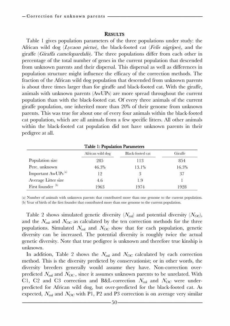
-------------------- C o r r e c t i o n f o r u n k n o w n p a r e n t s C o r r e c t i o n f o r u n k n o w n p a r e n t s C o r r e c t i o n f o r u n k n o w n p a r e n t s C o r r e c t i o n f o r u n k n o w n p a r e n t s ----------------------------------------------------------------------------------------------------------------------------------------------------------------------------------------------------------------------------------------------------------------------------------------------------------------------------------------------------------------------------------------------------------------------------------------------------------------------------------------------------------------------------------------------------------------------------------------------------------------------------------------------------------------------------------------
-------------------------------------------------------------------------------------------------------------------------------------------------------------------------------------------------------------------------------------------------------------------------------------------------------------------------------------------------------------------------------------------------------------------------------------------------------------------------------------------------------------------------------------------------------------------------------------------------------------------------------------------- ----------------------------------------------------------------------------------------------------------------------------------------------------------------------------------------------------------------------------------------------------------------------------------------------------------------------------------------------------------------------------------------------------------------------------------------------------------------------------------------------------------------------------------------------------------------------------------------------------------------
50
RRRRESULTSESULTSESULTSESULTS Table 1 gives population parameters of the three populations under study: the
African wild dog (Lycaon pictus), the black-footed cat (Felis nigripes), and the giraffe (Giraffa camelopardalis). The three populations differ from each other in percentage of the total number of genes in the current population that descended from unknown parents and their dispersal. This dispersal as well as differences in population structure might influence the efficacy of the correction methods. The fraction of the African wild dog population that descended from unknown parents is about three times larger than for giraffe and black-footed cat. With the giraffe, animals with unknown parents (AwUPs) are more spread throughout the current population than with the black-footed cat. Of every three animals of the current giraffe population, one inherited more than 20% of their genome from unknown parents. This was true for about one of every four animals within the black-footed cat population, which are all animals from a few specific litters. All other animals within the black-footed cat population did not have unknown parents in their pedigree at all.
Table 1: Population ParametersTable 1: Population ParametersTable 1: Population ParametersTable 1: Population Parameters
African wild dog Black-footed cat Giraffe
Population size 285 113 854 Perc. unknown 46.3% 13.1% 16.3% Important AwUPs (a) 12 3 37 Average Litter size 4.6 1.9 1 First founder (b) 1963 1974 1928
(a) Number of animals with unknown parents that contributed more than one genome to the current population. (b) Year of birth of the first founder that contributed more than one genome to the current population.
Table 2 shows simulated genetic diversity (Nmk) and potential diversity (NOC),
and the Nmk and NOC as calculated by the ten correction methods for the three populations. Simulated Nmk and NOC show that for each population, genetic diversity can be increased. The potential diversity is roughly twice the actual genetic diversity. Note that true pedigree is unknown and therefore true kinship is unknown.
In addition, Table 2 shows the Nmk and NOC calculated by each correction method. This is the diversity predicted by conservationist; or in other words, the diversity breeders generally would assume they have. Non-correction over-predicted Nmk and NOC , since it assumes unknown parents to be unrelated. With C1, C2 and C3 correction and B&L-correction Nmk and NOC were under-predicted for African wild dog, but over-predicted for the black-footed cat. As expected, Nmk and NOC with P1, P2 and P3 correction is on average very similar
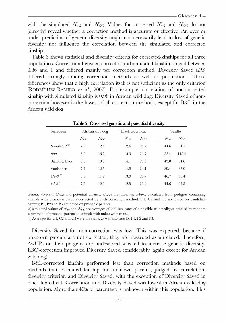
------------------------------------------------------------------------------------------------------------------------------------------------------------------------------------------------------------------------------------------------------------------------------------------------------------------------------------------------------------------------------------------------------------------------------------------------------------------------------------------------------------------------------------------------------------------------------------------------------------------------------------------------------------------------------------------------------------------------------------------------------------------------------------------------------------------------------------------------------------------------------------------------------------------------------------------------------------------------------------------------------------------------------------------------------------------------------------------------ C h a p t e r C h a p t e r C h a p t e r C h a p t e r 4444 --------------------
---------------------------------------------------------------------------------------------------------------------------------------------------------------------------------------------------------------------------------------------------------------------------------------------------------------------------------------------------------------------------------------------------------------------------------------------------------------------------------------------------------------------------------------------------------------------------------------------------------------------------------------- --------------------------------------------------------------------------------------------------------------------------------------------------------------------------------------------------------------------------------------------------------------------------------------------------------------------------------------------------------------------------------------------------------------------------------------------------------------------------------------------------------------------------------------------------------------------------------------------------------
51
with the simulated Nmk and NOC. Values for corrected Nmk and NOC do not (directly) reveal whether a correction method is accurate or effective. An over or under-prediction of genetic diversity might not necessarily lead to loss of genetic diversity nor influence the correlation between the simulated and corrected kinship.
Table 3 shows statistical and diversity criteria for corrected-kinships for all three populations. Correlation between corrected and simulated kinship ranged between 0.86 and 1 and differed mainly per correction method. Diversity Saved (DS) differed strongly among correction methods as well as populations. Those differences show that a high correlation itself is not sufficient as the only criterion (RODRÍGUEZ-RAMILO et al., 2007). For example, correlation of non-corrected kinship with simulated kinship is 0.98 in African wild dog. Diversity Saved of non-correction however is the lowest of all correction methods, except for B&L in the African wild dog
Table 2: Observed genetic and potential diversityTable 2: Observed genetic and potential diversityTable 2: Observed genetic and potential diversityTable 2: Observed genetic and potential diversity
correction African wild dog Black-footed cat Giraffe
Nmk NOC Nmk NOC Nmk NOC
Simulated (a) 7.2 12.4 12.6 23.2 44.6 94.1
non 8.9 16.7 15.3 24.7 53.4 115.4
Ballou & Lacy 5.6 10.5 14.1 22.9 43.8 94.6
VanRaden 7.5 12.5 14.9 24.1 39.4 87.0
C1-3 *2 6.5 11.9 13.9 23.7 46.7 95.4
P1-3 *2 7.2 12.1 12.5 23.2 44.6 93.3
Genetic diversity (Nmk) and potential diversity (NOC) are observed values, calculated from pedigree containing animals with unknown parents corrected by each correction method. C1, C2 and C3 are based on candidate parents; P1, P2 and P3 are based on probable parents. (a) simulated values of Nmk and NOC are averages of 200 replicates of a possible true pedigree created by random assignment of probable parents to animals with unknown parents. (b) Averages for C1, C2 and C3 were the same, as was also true for P1, P2 and P3.
Diversity Saved for non-correction was low. This was expected, because if
unknown parents are not corrected, they are regarded as unrelated. Therefore, AwUPs or their progeny are undeserved selected to increase genetic diversity. EBO-correction improved Diversity Saved considerably (again except for African wild dog).
B&L-corrected kinship performed less than correction methods based on methods that estimated kinship for unknown parents, judged by correlation, diversity criterion and Diversity Saved, with the exception of Diversity Saved in black-footed cat. Correlation and Diversity Saved was lowest in African wild dog population. More than 40% of parentage is unknown within this population. This
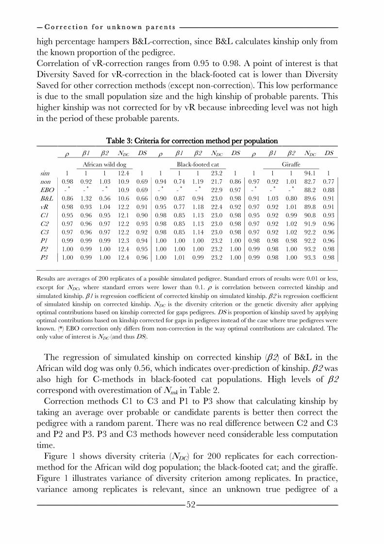
-------------------- C o r r e c t i o n f o r u n k n o w n p a r e n t s C o r r e c t i o n f o r u n k n o w n p a r e n t s C o r r e c t i o n f o r u n k n o w n p a r e n t s C o r r e c t i o n f o r u n k n o w n p a r e n t s ----------------------------------------------------------------------------------------------------------------------------------------------------------------------------------------------------------------------------------------------------------------------------------------------------------------------------------------------------------------------------------------------------------------------------------------------------------------------------------------------------------------------------------------------------------------------------------------------------------------------------------------------------------------------------------------
-------------------------------------------------------------------------------------------------------------------------------------------------------------------------------------------------------------------------------------------------------------------------------------------------------------------------------------------------------------------------------------------------------------------------------------------------------------------------------------------------------------------------------------------------------------------------------------------------------------------------------------------- ----------------------------------------------------------------------------------------------------------------------------------------------------------------------------------------------------------------------------------------------------------------------------------------------------------------------------------------------------------------------------------------------------------------------------------------------------------------------------------------------------------------------------------------------------------------------------------------------------------------
52
high percentage hampers B&L-correction, since B&L calculates kinship only from the known proportion of the pedigree. Correlation of vR-correction ranges from 0.95 to 0.98. A point of interest is that Diversity Saved for vR-correction in the black-footed cat is lower than Diversity Saved for other correction methods (except non-correction). This low performance is due to the small population size and the high kinship of probable parents. This higher kinship was not corrected for by vR because inbreeding level was not high in the period of these probable parents.
Table 3: Table 3: Table 3: Table 3: Criteria for correction method Criteria for correction method Criteria for correction method Criteria for correction method per populationper populationper populationper population
ρ β1 β2 NDC DS ρ β1 β2 NDC DS ρ β1 β2 NDC DS
African wild dog Black-footed cat Giraffe sim 1 1 1 12.4 1 1 1 1 23.2 1 1 1 1 94.1 1 non 0.98 0.92 1.03 10.9 0.69 0.94 0.74 1.19 21.7 0.86 0.97 0.92 1.01 82.7 0.77 EBO - * - * - * 10.9 0.69 - * - * - * 22.9 0.97 - * - * - * 88.2 0.88 B&L 0.86 1.32 0.56 10.6 0.66 0.90 0.87 0.94 23.0 0.98 0.91 1.03 0.80 89.6 0.91 vR 0.98 0.93 1.04 12.2 0.91 0.95 0.77 1.18 22.4 0.92 0.97 0.92 1.01 89.8 0.91 C1 0.95 0.96 0.95 12.1 0.90 0.98 0.85 1.13 23.0 0.98 0.95 0.92 0.99 90.8 0.93 C2 0.97 0.96 0.97 12.2 0.93 0.98 0.85 1.13 23.0 0.98 0.97 0.92 1.02 91.9 0.96 C3 0.97 0.96 0.97 12.2 0.92 0.98 0.85 1.14 23.0 0.98 0.97 0.92 1.02 92.2 0.96 P1 0.99 0.99 0.99 12.3 0.94 1.00 1.00 1.00 23.2 1.00 0.98 0.98 0.98 92.2 0.96 P2 1.00 0.99 1.00 12.4 0.95 1.00 1.00 1.00 23.2 1.00 0.99 0.98 1.00 93.2 0.98 P3 1.00 0.99 1.00 12.4 0.96 1.00 1.01 0.99 23.2 1.00 0.99 0.98 1.00 93.3 0.98
Results are averages of 200 replicates of a possible simulated pedigree. Standard errors of results were 0.01 or less, except for NDC, where standard errors were lower than 0.1. ρ is correlation between corrected kinship and simulated kinship. β1 is regression coefficient of corrected kinship on simulated kinship. β2 is regression coefficient of simulated kinship on corrected kinship. NDC is the diversity criterion or the genetic diversity after applying optimal contributions based on kinship corrected for gaps pedigrees. DS is proportion of kinship saved by applying optimal contributions based on kinship corrected for gaps in pedigrees instead of the case where true pedigrees were known. (*) EBO correction only differs from non-correction in the way optimal contributions are calculated. The only value of interest is NDC (and thus DS).
The regression of simulated kinship on corrected kinship (β2) of B&L in the African wild dog was only 0.56, which indicates over-prediction of kinship. β2 was also high for C-methods in black-footed cat populations. High levels of β2 correspond with overestimation of Nmk in Table 2.
Correction methods C1 to C3 and P1 to P3 show that calculating kinship by taking an average over probable or candidate parents is better then correct the pedigree with a random parent. There was no real difference between C2 and C3 and P2 and P3. P3 and C3 methods however need considerable less computation time.
Figure 1 shows diversity criteria (NDC) for 200 replicates for each correction-method for the African wild dog population; the black-footed cat; and the giraffe. Figure 1 illustrates variance of diversity criterion among replicates. In practice, variance among replicates is relevant, since an unknown true pedigree of a
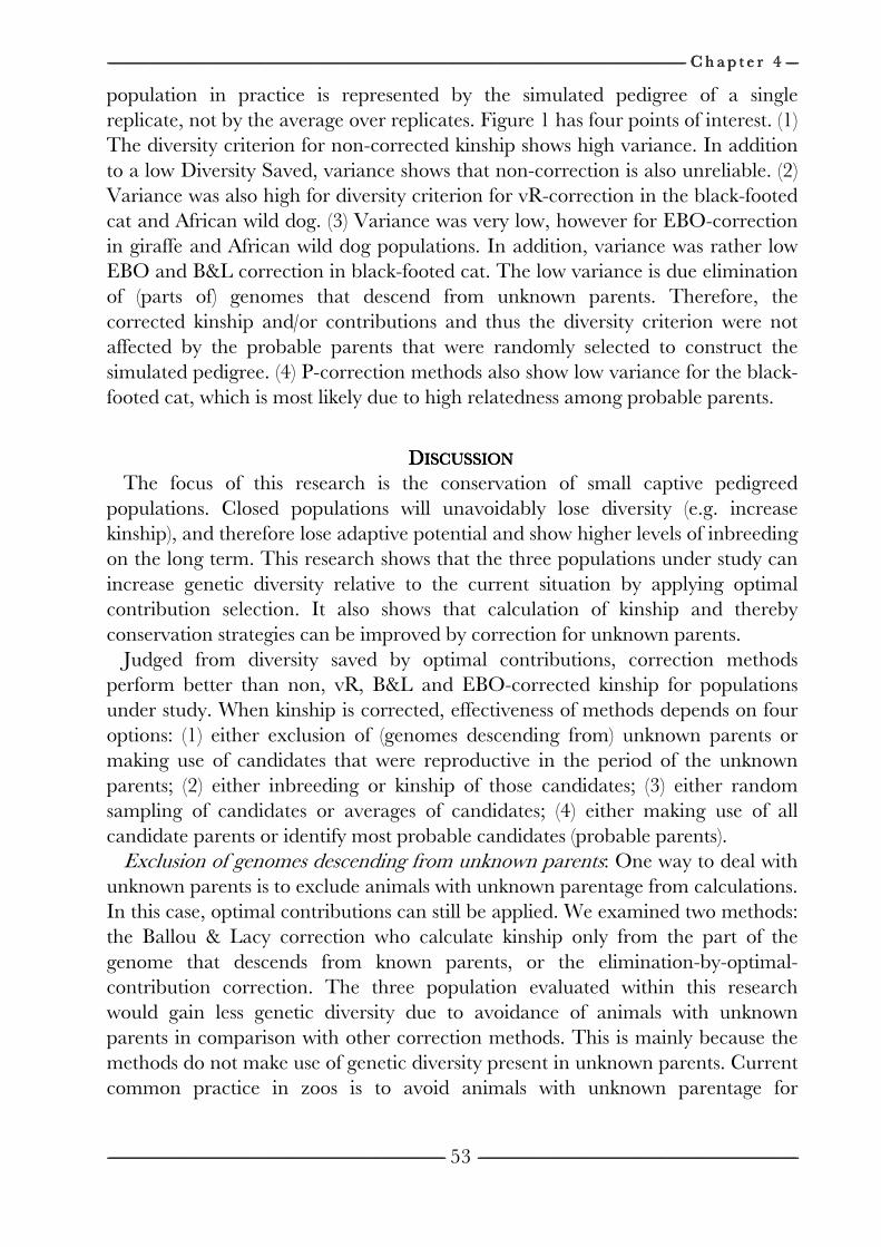
------------------------------------------------------------------------------------------------------------------------------------------------------------------------------------------------------------------------------------------------------------------------------------------------------------------------------------------------------------------------------------------------------------------------------------------------------------------------------------------------------------------------------------------------------------------------------------------------------------------------------------------------------------------------------------------------------------------------------------------------------------------------------------------------------------------------------------------------------------------------------------------------------------------------------------------------------------------------------------------------------------------------------------------------------------------------------------------------ C h a p t e r C h a p t e r C h a p t e r C h a p t e r 4444 --------------------
---------------------------------------------------------------------------------------------------------------------------------------------------------------------------------------------------------------------------------------------------------------------------------------------------------------------------------------------------------------------------------------------------------------------------------------------------------------------------------------------------------------------------------------------------------------------------------------------------------------------------------------- --------------------------------------------------------------------------------------------------------------------------------------------------------------------------------------------------------------------------------------------------------------------------------------------------------------------------------------------------------------------------------------------------------------------------------------------------------------------------------------------------------------------------------------------------------------------------------------------------------
53
population in practice is represented by the simulated pedigree of a single replicate, not by the average over replicates. Figure 1 has four points of interest. (1) The diversity criterion for non-corrected kinship shows high variance. In addition to a low Diversity Saved, variance shows that non-correction is also unreliable. (2) Variance was also high for diversity criterion for vR-correction in the black-footed cat and African wild dog. (3) Variance was very low, however for EBO-correction in giraffe and African wild dog populations. In addition, variance was rather low EBO and B&L correction in black-footed cat. The low variance is due elimination of (parts of) genomes that descend from unknown parents. Therefore, the corrected kinship and/or contributions and thus the diversity criterion were not affected by the probable parents that were randomly selected to construct the simulated pedigree. (4) P-correction methods also show low variance for the black-footed cat, which is most likely due to high relatedness among probable parents.
DDDDISCUSSIONISCUSSIONISCUSSIONISCUSSION The focus of this research is the conservation of small captive pedigreed
populations. Closed populations will unavoidably lose diversity (e.g. increase kinship), and therefore lose adaptive potential and show higher levels of inbreeding on the long term. This research shows that the three populations under study can increase genetic diversity relative to the current situation by applying optimal contribution selection. It also shows that calculation of kinship and thereby conservation strategies can be improved by correction for unknown parents.
Judged from diversity saved by optimal contributions, correction methods perform better than non, vR, B&L and EBO-corrected kinship for populations under study. When kinship is corrected, effectiveness of methods depends on four options: (1) either exclusion of (genomes descending from) unknown parents or making use of candidates that were reproductive in the period of the unknown parents; (2) either inbreeding or kinship of those candidates; (3) either random sampling of candidates or averages of candidates; (4) either making use of all candidate parents or identify most probable candidates (probable parents).
Exclusion of genomes descending from unknown parents: One way to deal with unknown parents is to exclude animals with unknown parentage from calculations. In this case, optimal contributions can still be applied. We examined two methods: the Ballou & Lacy correction who calculate kinship only from the part of the genome that descends from known parents, or the elimination-by-optimal-contribution correction. The three population evaluated within this research would gain less genetic diversity due to avoidance of animals with unknown parents in comparison with other correction methods. This is mainly because the methods do not make use of genetic diversity present in unknown parents. Current common practice in zoos is to avoid animals with unknown parentage for
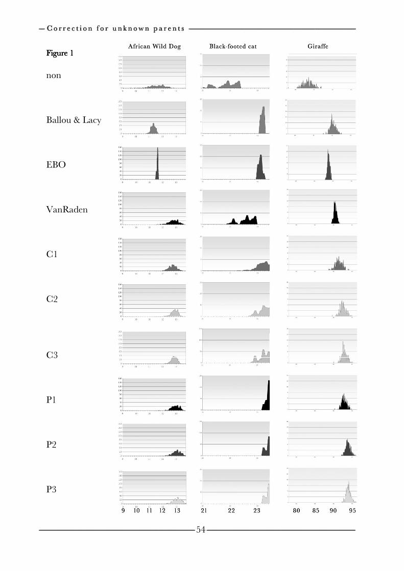
-------------------- C o r r e c t i o n f o r u n k n o w n p a r e n t s C o r r e c t i o n f o r u n k n o w n p a r e n t s C o r r e c t i o n f o r u n k n o w n p a r e n t s C o r r e c t i o n f o r u n k n o w n p a r e n t s
----------------------------------------------------------------------------------------------------------------------------------------------------------------------------------------------------------------------------------------------------------------------------------------------------------------------------------------------------------------------------------------------------------------------------------------------------------------------------------------
Figure 1Figure 1Figure 1Figure 1
non Ballou & Lacy EBO VanRaden C1 C2 C3 P1 P2 P3
C o r r e c t i o n f o r u n k n o w n p a r e n t s C o r r e c t i o n f o r u n k n o w n p a r e n t s C o r r e c t i o n f o r u n k n o w n p a r e n t s C o r r e c t i o n f o r u n k n o w n p a r e n t s
----------------------------------------------------------------------------------------------------------------------------------------------------------------------------------------------------------------------------------------------------------------------------------------------------------------------------------------------------------------------------------------------------------------------------------------------------------------------------------------
Figure 1Figure 1Figure 1Figure 1
Ballou & Lacy
VanRaden
C o r r e c t i o n f o r u n k n o w n p a r e n t s C o r r e c t i o n f o r u n k n o w n p a r e n t s C o r r e c t i o n f o r u n k n o w n p a r e n t s C o r r e c t i o n f o r u n k n o w n p a r e n t s
----------------------------------------------------------------------------------------------------------------------------------------------------------------------------------------------------------------------------------------------------------------------------------------------------------------------------------------------------------------------------------------------------------------------------------------------------------------------------------------
C o r r e c t i o n f o r u n k n o w n p a r e n t s C o r r e c t i o n f o r u n k n o w n p a r e n t s C o r r e c t i o n f o r u n k n o w n p a r e n t s C o r r e c t i o n f o r u n k n o w n p a r e n t s
----------------------------------------------------------------------------------------------------------------------------------------------------------------------------------------------------------------------------------------------------------------------------------------------------------------------------------------------------------------------------------------------------------------------------------------------------------------------------------------------------------------------------------------------------------------------------------------------------------------
C o r r e c t i o n f o r u n k n o w n p a r e n t s C o r r e c t i o n f o r u n k n o w n p a r e n t s C o r r e c t i o n f o r u n k n o w n p a r e n t s C o r r e c t i o n f o r u n k n o w n p a r e n t s --------------------------------------------------------------------------------------------------------------------------------------------------------------------------------------------------------------------------------------------------------------------------------------------------------------------------------------------------------------------------------------------------------------------------------------------------------------------------------------------------------------------
---------------------------------------------------------------------------------------------------------------------------------------------------- --------------------------------------------------------------------------------------------------------------------------------------------------------------------------------------------------------------------------------54
--------------------------------------------------------------------------------------------------------------------------------------------------------------------------------------------------------------------------------------------------------------------------------------------------------------------------------------------------------------------------------------------------------------------------------------------------------------------------------------------------------------------
--------------------------------------------------------------------------------------------------------------------------------------------------------------------------------------------------------------------------------
--------------------------------------------------------------------------------------------------------------------------------------------------------------------------------------------------------------------------------------------------------------------------------------------------------------------------------------------------------------------------------------------------------------------------------------------------------------------------------------------------------------------
----------------------------------------------------------------------------------------------------------------------------------------------------------------------------------------------------------------------------------------------------------------------------------------------------------------------------------------------------------------------------------------------------------------------------------------------------------------------------------------------------------------------------------------------------------------------------------------------------------------
----------------------------------------------------------------------------------------------------------------------------------------------------------------------------------------------------------------------------------------------------------------------------------------------------------------------------------------------------------------------------------------------------------------------------------------------------------------------------------------------------------------------------------------------------------------------------------------------------------------------------------------------------------------------------------------
--------------------------------------------------------------------------------------------------------------------------------------------------------------------------------------------------------------------------------------------------------------------------------------------
--------------------------------------------------------------------------------------------------------------------------------------------------------------------
--------------------------------------------------------------------------------------------------------------------------------------------------------------------------------------------------------------------------------------------------------------------------------------------
------------------------------------------------------------------------------------------------------------------------------------------------------------------------------------------------------------------------------------------------------------------------------------------------------------------------------------------------------------------------------------------------------------------------------------------------------------------------------------------------------------------------------------------------------------------------------------------------------------------------------------------------------------------------------------------------------------------------------------------------------------------------------------------------------------------------------------------------------------------------------------------------------------------------------------------------------------------------------------------------------------------------------------------------------------------------------------------------ C h a p t e r C h a p t e r C h a p t e r C h a p t e r 4444 --------------------
---------------------------------------------------------------------------------------------------------------------------------------------------------------------------------------------------------------------------------------------------------------------------------------------------------------------------------------------------------------------------------------------------------------------------------------------------------------------------------------------------------------------------------------------------------------------------------------------------------------------------------------- --------------------------------------------------------------------------------------------------------------------------------------------------------------------------------------------------------------------------------------------------------------------------------------------------------------------------------------------------------------------------------------------------------------------------------------------------------------------------------------------------------------------------------------------------------------------------------------------------------
55
breeding. A potential gain of genetic diversity declines by this policy. Exclusion of animals with unknown parentage from conservation should only be favored over other methods when unknown parents would cause undesirable introgression (for example among subspecies). The elimination-by-optimal-contribution correction is than preferred because it is probably more efficient in eliminating genomes descending from unknown parents, since it shows lowest variance in the diversity criterion.
Inbreeding or kinship: vanRaden correction made use of inbreeding to correct for unknown parents within kinship calculations. In pedigrees like EEP-studbooks due to small population size and relative low number of generations, the average inbreeding may differ considerably from average mean kinship. Especially in the first generations, inbreeding is low or even zero. This explains the low performance of vanRaden-correction in black-footed cat population, which is the smallest of the three populations. With current computation power, there is no reason to use inbreeding instead of kinship to correct for unknown parents. Thus, the level of kinship of parents is preferred to correct for unknown parents, not the level of inbreeding.
Random sampling or taking average: This research compared three ways to correct kinship from possible parents for animals with unknown parents: (1) assigning a random parent for each unknown parent (C1 and P1 correction); (2) assigning random parents for twenty times (C2 and P2 correction); and taking average of possible parents (C3 and P3 correction). Assigning a random parent or taking average from possible parents was more efficient in computation-time than assigning random parents for twenty times. Averaging kinship of possible parents and assigning random possible parents for twenty times performed more effective in conservation of genetic diversity than assigning a random parent. Hence, repetitive random sampling does not improve conservation compared to taking averages. Taking averages over possible parents (either candidate or probable) parents is both effective and efficient.
Specification of probable parents: To identify probable parents, only animals with unknown parents that have descendants in the current population were selected. Next, species coordinators determined probable parents, which was a time-consuming process. They used knowledge on common exchange practices, which differ over time, zoos and countries. Where available, recorded additional information was used, like the names of possible candidate males. Choices of species coordinators were not always obvious for an outsider. Hence, inside knowledge is necessary to identify probable parents. When multiple parents are registered, this correction-method can be applied quickly. Determining probable parents per animal with unknown parents, however, is a time-costly process. Whether or not probably parents should be identified, (C3 vs. P3 correction) is less
-------------------- C o r r e c t i o n f o r u n k n o w n p a r e n t s C o r r e c t i o n f o r u n k n o w n p a r e n t s C o r r e c t i o n f o r u n k n o w n p a r e n t s C o r r e c t i o n f o r u n k n o w n p a r e n t s ----------------------------------------------------------------------------------------------------------------------------------------------------------------------------------------------------------------------------------------------------------------------------------------------------------------------------------------------------------------------------------------------------------------------------------------------------------------------------------------------------------------------------------------------------------------------------------------------------------------------------------------------------------------------------------------
-------------------------------------------------------------------------------------------------------------------------------------------------------------------------------------------------------------------------------------------------------------------------------------------------------------------------------------------------------------------------------------------------------------------------------------------------------------------------------------------------------------------------------------------------------------------------------------------------------------------------------------------- ----------------------------------------------------------------------------------------------------------------------------------------------------------------------------------------------------------------------------------------------------------------------------------------------------------------------------------------------------------------------------------------------------------------------------------------------------------------------------------------------------------------------------------------------------------------------------------------------------------------
56
evident, especially because the process is time-consuming. Though the effort could improve genetic diversity saved, the extra gain is low.
A combined C3-P3 correction was applied on giraffe and African wild dog population. For giraffe, only twelve AwUPs contributed for more than 50% of total number of genomes that descended from AwUPs. For African wild dog, only three AwUPs contributed for more than 50%. Kinship for those twelve giraffe and three African wild dogs with unknown parents were P3 corrected, while kinships of all other animals with unknown parents were C3 corrected. This combined C3-P3 correction hardly showed any decrease for DS in comparison with the P3 correction for the same populations. These results indicate that conservation of genetic diversity already benefits from determining probable parents only for few AwUPs that have contributed for 50% to the current population. We advise to determine probable parents only for AwUPs that contributed most to the current population. In conclusion, correction for unknown parents by taking average of manually selected probable parents for animals with high impact on the current population and automatically selected candidate parents for all other animals is an effective and efficient strategy.
AAAACKNOWLEDGEMENTCKNOWLEDGEMENTCKNOWLEDGEMENTCKNOWLEDGEMENT I thank Marc Damen, Lars Versteege, Jacques Kaandorp, Hanny Verberkmoes,
Martin van Wees and André Stadler for making data available and going through the effort of assigning probable parents to each animal with unknown parents.
----------------------------------------------------------------------------------------------------------------------------------------------------------------------------------------------------------------------------------------------------------------------------------------------------------------------------------------------------------------------------------------------------------------------------------------------------------------------------------------------------------------------------------------------------------------------------------------------------------------------------------------------------------------------------------------------------------------------------------------------------------------------------------------------------------------------------------------------------------------------------------------------------------------------------------------------------------------------------------------------------------------------------------------------------------------------------------------------------------------------------------------------------------------------------------------------------------------------------------------------------------------------------------------------------------------
-------------------------------------------------------------------------------------------------------------------------------------------------------------------------------------------------------------------------------------------------------------------------------------------------------------------------------------------------------------------------------------------------------------------------------------------------------------------------------------------------------------------------------------------------------------------------------------------------------------------------------------------- ----------------------------------------------------------------------------------------------------------------------------------------------------------------------------------------------------------------------------------------------------------------------------------------------------------------------------------------------------------------------------------------------------------------------------------------------------------------------------------------------------------------------------------------------------------------------------------------------------------------
57
Estimating relatedness between individuals Estimating relatedness between individuals Estimating relatedness between individuals Estimating relatedness between individuals
in general populationsin general populationsin general populationsin general populations
with a focus on their use in conservation programswith a focus on their use in conservation programswith a focus on their use in conservation programswith a focus on their use in conservation programs
C h a p t e r C h a p t e r C h a p t e r C h a p t e r 5555
Pieter Oliehoek, * Jack Windig, ‡, Johan van Arendonk * and Piter Bijma *
* Animal Breeding and Genetics, Wageningen University, The Netherlands
‡ Centre for Genetic Resources, the Netherlands (CGN) Wageningen University, The Netherlands
Published in Genetics (2006) 173173173173: 483-496.
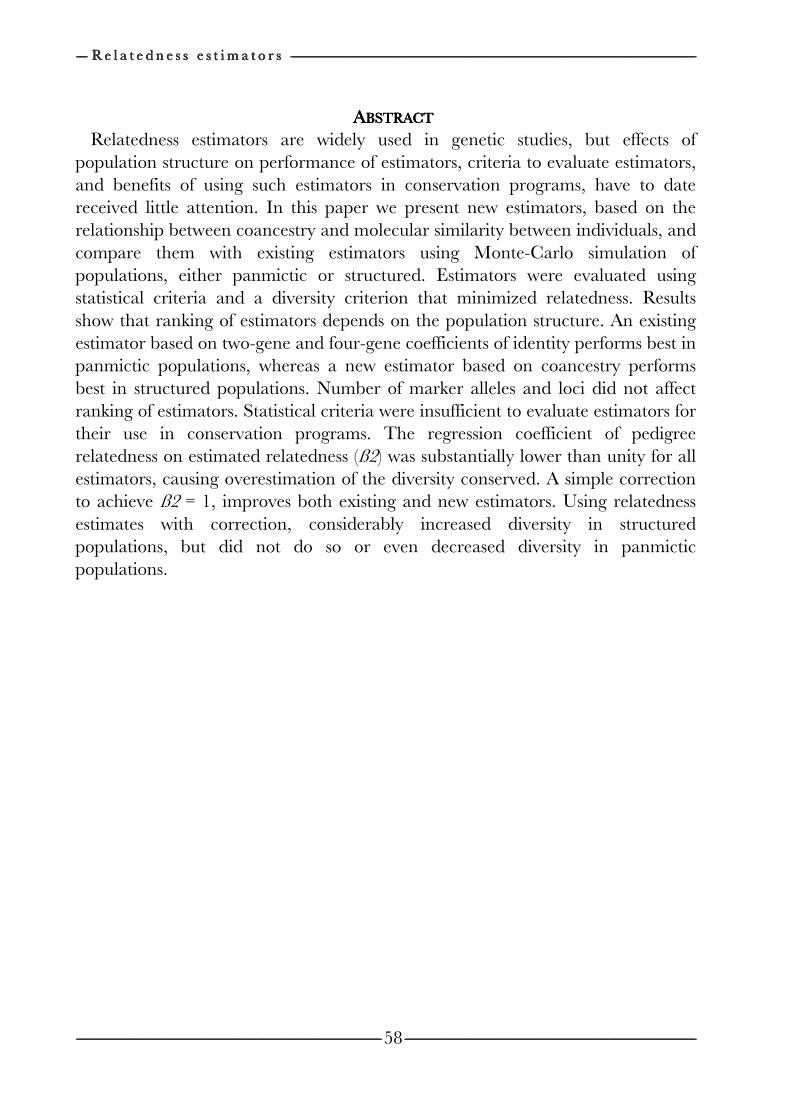
-------------------- R e l a t e d n e s s e s t i m a t o r s R e l a t e d n e s s e s t i m a t o r s R e l a t e d n e s s e s t i m a t o r s R e l a t e d n e s s e s t i m a t o r s --------------------------------------------------------------------------------------------------------------------------------------------------------------------------------------------------------------------------------------------------------------------------------------------------------------------------------------------------------------------------------------------------------------------------------------------------------------------------------------------------------------------------------------------------------------------------------------------------------------------------------------------------------------------------------------------------------------------------------------------------------------------------------------------------------------------------------------------------------
-------------------------------------------------------------------------------------------------------------------------------------------------------------------------------------------------------------------------------------------------------------------------------------------------------------------------------------------------------------------------------------------------------------------------------------------------------------------------------------------------------------------------------------------------------------------------------------------------------------------------------------------- ----------------------------------------------------------------------------------------------------------------------------------------------------------------------------------------------------------------------------------------------------------------------------------------------------------------------------------------------------------------------------------------------------------------------------------------------------------------------------------------------------------------------------------------------------------------------------------------------------------------
58
AAAABSTRACTBSTRACTBSTRACTBSTRACT Relatedness estimators are widely used in genetic studies, but effects of
population structure on performance of estimators, criteria to evaluate estimators, and benefits of using such estimators in conservation programs, have to date received little attention. In this paper we present new estimators, based on the relationship between coancestry and molecular similarity between individuals, and compare them with existing estimators using Monte-Carlo simulation of populations, either panmictic or structured. Estimators were evaluated using statistical criteria and a diversity criterion that minimized relatedness. Results show that ranking of estimators depends on the population structure. An existing estimator based on two-gene and four-gene coefficients of identity performs best in panmictic populations, whereas a new estimator based on coancestry performs best in structured populations. Number of marker alleles and loci did not affect ranking of estimators. Statistical criteria were insufficient to evaluate estimators for their use in conservation programs. The regression coefficient of pedigree relatedness on estimated relatedness (ß2) was substantially lower than unity for all estimators, causing overestimation of the diversity conserved. A simple correction to achieve ß2 = 1, improves both existing and new estimators. Using relatedness estimates with correction, considerably increased diversity in structured populations, but did not do so or even decreased diversity in panmictic populations.
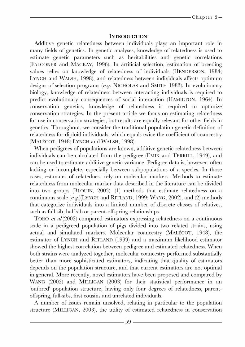
------------------------------------------------------------------------------------------------------------------------------------------------------------------------------------------------------------------------------------------------------------------------------------------------------------------------------------------------------------------------------------------------------------------------------------------------------------------------------------------------------------------------------------------------------------------------------------------------------------------------------------------------------------------------------------------------------------------------------------------------------------------------------------------------------------------------------------------------------------------------------------------------------------------------------------------------------------------------------------------------------------------------------------------------------------------------------------------------ C h a p t e r C h a p t e r C h a p t e r C h a p t e r 5555 --------------------
---------------------------------------------------------------------------------------------------------------------------------------------------------------------------------------------------------------------------------------------------------------------------------------------------------------------------------------------------------------------------------------------------------------------------------------------------------------------------------------------------------------------------------------------------------------------------------------------------------------------------------------- --------------------------------------------------------------------------------------------------------------------------------------------------------------------------------------------------------------------------------------------------------------------------------------------------------------------------------------------------------------------------------------------------------------------------------------------------------------------------------------------------------------------------------------------------------------------------------------------------------
59
IIIINTRODUCTIONNTRODUCTIONNTRODUCTIONNTRODUCTION Additive genetic relatedness between individuals plays an important role in
many fields of genetics. In genetic analyses, knowledge of relatedness is used to estimate genetic parameters such as heritabilities and genetic correlations (FALCONER and MACKAY, 1996). In artificial selection, estimation of breeding values relies on knowledge of relatedness of individuals (HENDERSON, 1984; LYNCH and WALSH, 1998), and relatedness between individuals affects optimum designs of selection programs (e.g. NICHOLAS and SMITH 1983). In evolutionary biology, knowledge of relatedness between interacting individuals is required to predict evolutionary consequences of social interaction (HAMILTON, 1964). In conservation genetics, knowledge of relatedness is required to optimize conservation strategies. In the present article we focus on estimating relatedness for use in conservation strategies, but results are equally relevant for other fields in genetics. Throughout, we consider the traditional population-genetic definition of relatedness for diploid individuals, which equals twice the coefficient of coancestry (MALÉCOT, 1948; LYNCH and WALSH, 1998).
When pedigrees of populations are known, additive genetic relatedness between individuals can be calculated from the pedigree (EMIK and TERRILL, 1949), and can be used to estimate additive genetic variance. Pedigree data is, however, often lacking or incomplete, especially between subpopulations of a species. In those cases, estimates of relatedness rely on molecular markers. Methods to estimate relatedness from molecular marker data described in the literature can be divided into two groups (BLOUIN, 2003): (1) methods that estimate relatedness on a continuous scale (e.g.)(LYNCH and RITLAND, 1999; WANG, 2002), and (2) methods that categorize individuals into a limited number of discrete classes of relatives, such as full sib, half sib or parent-offspring relationships.
TORO et al.(2002) compared estimators expressing relatedness on a continuous scale in a pedigreed population of pigs divided into two related strains, using actual and simulated markers. Molecular coancestry (MALÉCOT, 1948), the estimator of LYNCH and RITLAND (1999) and a maximum likelihood estimator showed the highest correlation between pedigree and estimated relatedness. When both strains were analyzed together, molecular coancestry performed substantially better than more sophisticated estimators, indicating that quality of estimators depends on the population structure, and that current estimators are not optimal in general. More recently, novel estimators have been proposed and compared by WANG (2002) and MILLIGAN (2003) for their statistical performance in an 'outbred' population structure, having only four degrees of relatedness, parent-offspring, full-sibs, first cousins and unrelated individuals.
A number of issues remain unsolved, relating in particular to the population structure (MILLIGAN, 2003), the utility of estimated relatedness in conservation
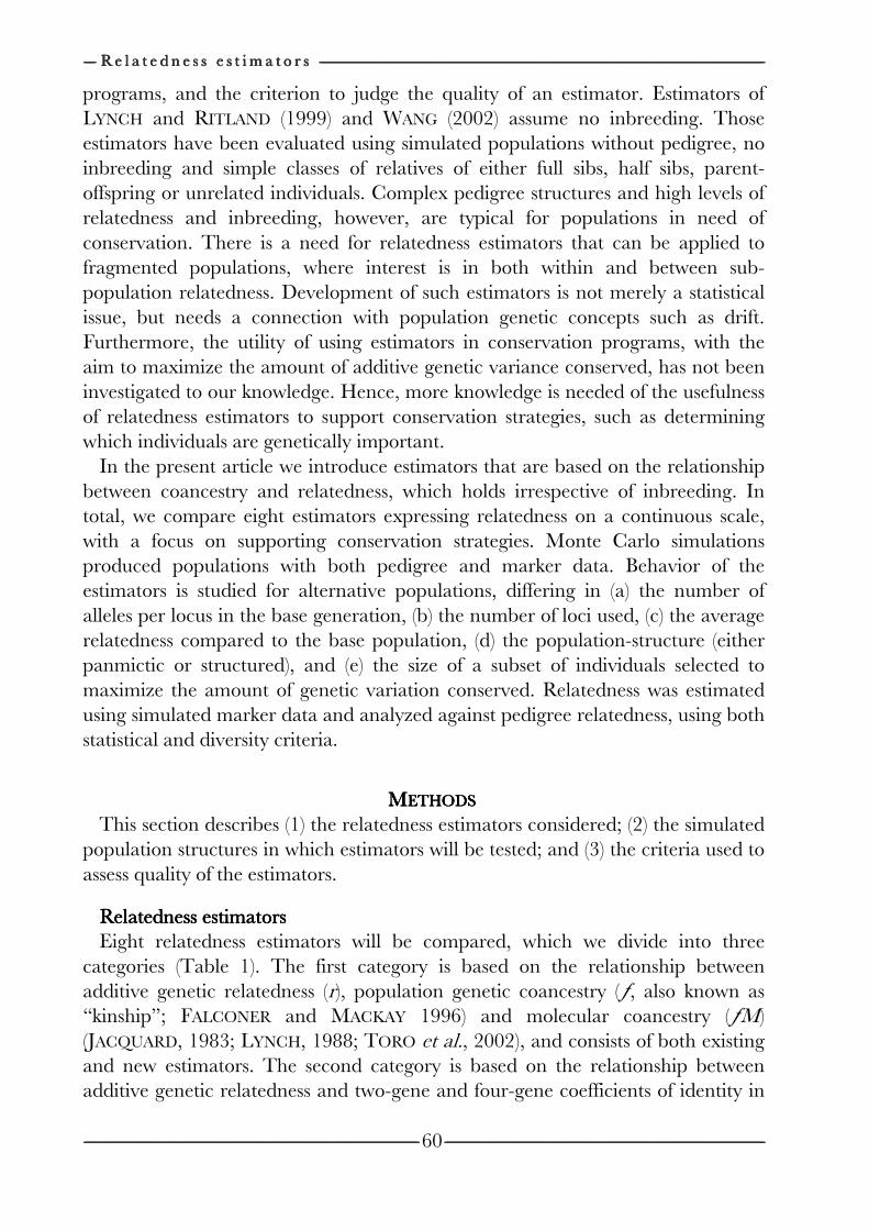
-------------------- R e l a t e d n e s s e s t i m a t o r s R e l a t e d n e s s e s t i m a t o r s R e l a t e d n e s s e s t i m a t o r s R e l a t e d n e s s e s t i m a t o r s --------------------------------------------------------------------------------------------------------------------------------------------------------------------------------------------------------------------------------------------------------------------------------------------------------------------------------------------------------------------------------------------------------------------------------------------------------------------------------------------------------------------------------------------------------------------------------------------------------------------------------------------------------------------------------------------------------------------------------------------------------------------------------------------------------------------------------------------------------
-------------------------------------------------------------------------------------------------------------------------------------------------------------------------------------------------------------------------------------------------------------------------------------------------------------------------------------------------------------------------------------------------------------------------------------------------------------------------------------------------------------------------------------------------------------------------------------------------------------------------------------------- ----------------------------------------------------------------------------------------------------------------------------------------------------------------------------------------------------------------------------------------------------------------------------------------------------------------------------------------------------------------------------------------------------------------------------------------------------------------------------------------------------------------------------------------------------------------------------------------------------------------
60
programs, and the criterion to judge the quality of an estimator. Estimators of LYNCH and RITLAND (1999) and WANG (2002) assume no inbreeding. Those estimators have been evaluated using simulated populations without pedigree, no inbreeding and simple classes of relatives of either full sibs, half sibs, parent-offspring or unrelated individuals. Complex pedigree structures and high levels of relatedness and inbreeding, however, are typical for populations in need of conservation. There is a need for relatedness estimators that can be applied to fragmented populations, where interest is in both within and between sub-population relatedness. Development of such estimators is not merely a statistical issue, but needs a connection with population genetic concepts such as drift. Furthermore, the utility of using estimators in conservation programs, with the aim to maximize the amount of additive genetic variance conserved, has not been investigated to our knowledge. Hence, more knowledge is needed of the usefulness of relatedness estimators to support conservation strategies, such as determining which individuals are genetically important.
In the present article we introduce estimators that are based on the relationship between coancestry and relatedness, which holds irrespective of inbreeding. In total, we compare eight estimators expressing relatedness on a continuous scale, with a focus on supporting conservation strategies. Monte Carlo simulations produced populations with both pedigree and marker data. Behavior of the estimators is studied for alternative populations, differing in (a) the number of alleles per locus in the base generation, (b) the number of loci used, (c) the average relatedness compared to the base population, (d) the population-structure (either panmictic or structured), and (e) the size of a subset of individuals selected to maximize the amount of genetic variation conserved. Relatedness was estimated using simulated marker data and analyzed against pedigree relatedness, using both statistical and diversity criteria.
MMMMETHODSETHODSETHODSETHODS This section describes (1) the relatedness estimators considered; (2) the simulated
population structures in which estimators will be tested; and (3) the criteria used to assess quality of the estimators.
Relatedness estimatorsRelatedness estimatorsRelatedness estimatorsRelatedness estimators Eight relatedness estimators will be compared, which we divide into three
categories (Table 1). The first category is based on the relationship between additive genetic relatedness (r), population genetic coancestry (ƒ, also known as “kinship”; FALCONER and MACKAY 1996) and molecular coancestry (ƒM) (JACQUARD, 1983; LYNCH, 1988; TORO et al., 2002), and consists of both existing and new estimators. The second category is based on the relationship between additive genetic relatedness and two-gene and four-gene coefficients of identity in
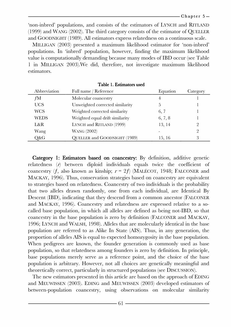
------------------------------------------------------------------------------------------------------------------------------------------------------------------------------------------------------------------------------------------------------------------------------------------------------------------------------------------------------------------------------------------------------------------------------------------------------------------------------------------------------------------------------------------------------------------------------------------------------------------------------------------------------------------------------------------------------------------------------------------------------------------------------------------------------------------------------------------------------------------------------------------------------------------------------------------------------------------------------------------------------------------------------------------------------------------------------------------------ C h a p t e r C h a p t e r C h a p t e r C h a p t e r 5555 --------------------
---------------------------------------------------------------------------------------------------------------------------------------------------------------------------------------------------------------------------------------------------------------------------------------------------------------------------------------------------------------------------------------------------------------------------------------------------------------------------------------------------------------------------------------------------------------------------------------------------------------------------------------- --------------------------------------------------------------------------------------------------------------------------------------------------------------------------------------------------------------------------------------------------------------------------------------------------------------------------------------------------------------------------------------------------------------------------------------------------------------------------------------------------------------------------------------------------------------------------------------------------------
61
‘non-inbred’ populations, and consists of the estimators of LYNCH and RITLAND (1999) and WANG (2002). The third category consists of the estimator of QUELLER and GOODNIGHT (1989). All estimators express relatedness on a continuous scale.
MILLIGAN (2003) presented a maximum likelihood estimator for ‘non-inbred’ populations. In ‘inbred’ population, however, finding the maximum likelihood value is computationally demanding because many modes of IBD occur (see Table 1 in MILLIGAN 2003).We did, therefore, not investigate maximum likelihood estimators.
Table 1. Estimators usedTable 1. Estimators usedTable 1. Estimators usedTable 1. Estimators used
Abbreviation Full name / Reference Equation Category
ƒM Molecular coancestry 4 1
UCS Unweighted corrected similarity 5 1
WCS Weighted corrected similarity 6, 7 1
WEDS Weighted equal drift similarity 6, 7, 8 1
L&R LYNCH and RITLAND (1999) 13, 14 2
Wang WANG (2002) - 2
Q&G QUELLER and GOODNIGHT (1989) 15, 16 3
Category 1: Estimators based on coancestry: Category 1: Estimators based on coancestry: Category 1: Estimators based on coancestry: Category 1: Estimators based on coancestry: By definition, additive genetic
relatedness (r) between diploid individuals equals twice the coefficient of coancestry (ƒ, also known as kinship; r = 2ƒ) (MALÉCOT, 1948; FALCONER and MACKAY, 1996). Thus, conservation strategies based on coancestry are equivalent to strategies based on relatedness. Coancestry of two individuals is the probability that two alleles drawn randomly, one from each individual, are Identical By Descent (IBD), indicating that they descend from a common ancestor (FALCONER and MACKAY, 1996). Coancestry and relatedness are expressed relative to a so-called base population, in which all alleles are defined as being not-IBD, so that coancestry in the base population is zero by definition (FALCONER and MACKAY, 1996; LYNCH and WALSH, 1998). Alleles that are molecularly identical in the base population are referred to as Alike In State (AIS). Thus, in any generation, the proportion of alleles AIS is equal to expected homozygosity in the base population. When pedigrees are known, the founder generation is commonly used as base population, so that relatedness among founders is zero by definition. In principle, base populations merely serve as a reference point, and the choice of the base population is arbitrary. However, not all choices are genetically meaningful and theoretically correct, particularly in structured populations (see DISCUSSION).
The new estimators presented in this article are based on the approach of EDING and MEUWISSEN (2003). EDING and MEUWISSEN (2003) developed estimators of between-population coancestry, using observations on molecular similarity
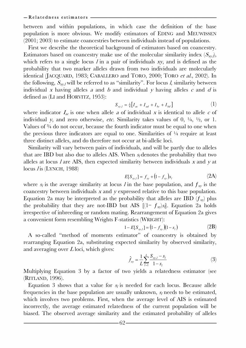
-------------------- R e l a t e d n e s s e s t i m a t o r s R e l a t e d n e s s e s t i m a t o r s R e l a t e d n e s s e s t i m a t o r s R e l a t e d n e s s e s t i m a t o r s --------------------------------------------------------------------------------------------------------------------------------------------------------------------------------------------------------------------------------------------------------------------------------------------------------------------------------------------------------------------------------------------------------------------------------------------------------------------------------------------------------------------------------------------------------------------------------------------------------------------------------------------------------------------------------------------------------------------------------------------------------------------------------------------------------------------------------------------------------
-------------------------------------------------------------------------------------------------------------------------------------------------------------------------------------------------------------------------------------------------------------------------------------------------------------------------------------------------------------------------------------------------------------------------------------------------------------------------------------------------------------------------------------------------------------------------------------------------------------------------------------------- ----------------------------------------------------------------------------------------------------------------------------------------------------------------------------------------------------------------------------------------------------------------------------------------------------------------------------------------------------------------------------------------------------------------------------------------------------------------------------------------------------------------------------------------------------------------------------------------------------------------
62
between and within populations, in which case the definition of the base population is more obvious. We modify estimators of EDING and MEUWISSEN (2001; 2003) to estimate coancestries between individuals instead of populations.
First we describe the theoretical background of estimators based on coancestry. Estimators based on coancestry make use of the molecular similarity index (Sxy,l), which refers to a single locus l in a pair of individuals xy, and is defined as the probability that two marker alleles drawn from two individuals are molecularly identical (JACQUARD, 1983; CABALLERO and TORO, 2000; TORO et al., 2002). In the following, Sxy,l will be referred to as “similarity”. For locus l, similarity between individual x having alleles a and b and individual y having alleles c and d is defined as (LI and HORVITZ, 1953):
[ ]bdbcadaclxy IIIIS +++=41
, ((11))
where indicator Iac is one when allele a of individual x is identical to allele c of individual y, and zero otherwise, etc. Similarity takes values of 0, ¼, ½, or 1. Values of ¾ do not occur, because the fourth indicator must be equal to one when the previous three indicators are equal to one. Similarities of ¼ require at least three distinct alleles, and do therefore not occur at bi-allelic loci.
Similarity will vary between pairs of individuals, and will be partly due to alleles that are IBD but also due to alleles AIS. When sl denotes the probability that two alleles at locus l are AIS, then expected similarity between individuals x and y at locus l is (LYNCH, 1988)
( ) lxyxylxy sffSE −+= 1][ , ((22AA))
where sl is the average similarity at locus l in the base population, and ƒxy is the coancestry between individuals x and y expressed relative to this base population. Equation 2a may be interpreted as the probability that alleles are IBD (ƒxy) plus the probability that they are not-IBD but AIS [(1− ƒxy)sl]. Equation 2a holds irrespective of inbreeding or random mating. Rearrangement of Equation 2a gives a convenient form resembling Wrights F-statistics (WRIGHT):
( )( )lxylxy sfSE −−=− 11][1 , ((22BB))
A so-called “method of moments estimator” of coancestry is obtained by rearranging Equation 2a, substituting expected similarity by observed similarity, and averaging over L loci, which gives:
∑= −
−=
L
l l
llxy
xys
sS
Lf
1
,
1
1ˆ ((33))
Multiplying Equation 3 by a factor of two yields a relatedness estimator (see (RITLAND, 1996).
Equation 3 shows that a value for sl is needed for each locus. Because allele frequencies in the base population are usually unknown, sl needs to be estimated, which involves two problems. First, when the average level of AIS is estimated incorrectly, the average estimated relatedness of the current population will be biased. The observed average similarity and the estimated probability of alleles
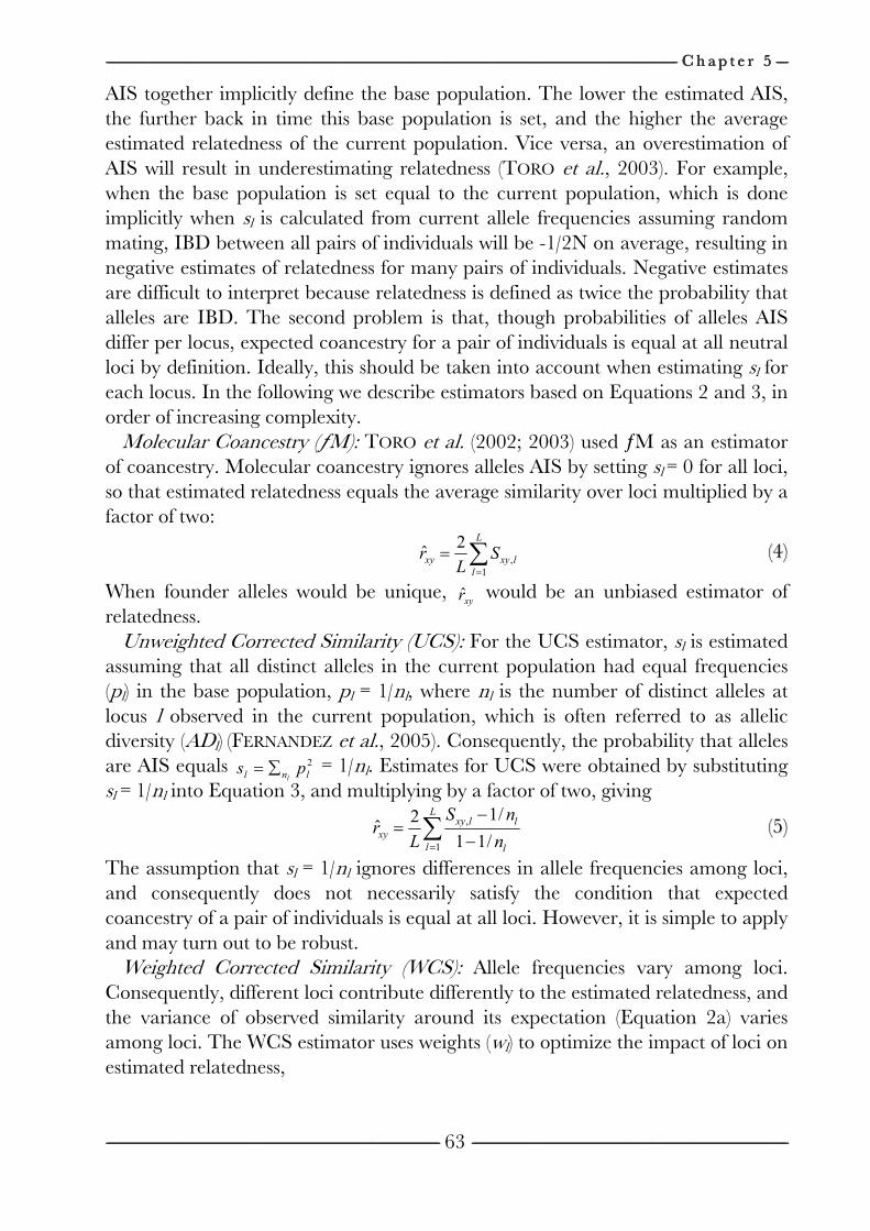
------------------------------------------------------------------------------------------------------------------------------------------------------------------------------------------------------------------------------------------------------------------------------------------------------------------------------------------------------------------------------------------------------------------------------------------------------------------------------------------------------------------------------------------------------------------------------------------------------------------------------------------------------------------------------------------------------------------------------------------------------------------------------------------------------------------------------------------------------------------------------------------------------------------------------------------------------------------------------------------------------------------------------------------------------------------------------------------------ C h a p t e r C h a p t e r C h a p t e r C h a p t e r 5555 --------------------
---------------------------------------------------------------------------------------------------------------------------------------------------------------------------------------------------------------------------------------------------------------------------------------------------------------------------------------------------------------------------------------------------------------------------------------------------------------------------------------------------------------------------------------------------------------------------------------------------------------------------------------- --------------------------------------------------------------------------------------------------------------------------------------------------------------------------------------------------------------------------------------------------------------------------------------------------------------------------------------------------------------------------------------------------------------------------------------------------------------------------------------------------------------------------------------------------------------------------------------------------------
63
AIS together implicitly define the base population. The lower the estimated AIS, the further back in time this base population is set, and the higher the average estimated relatedness of the current population. Vice versa, an overestimation of AIS will result in underestimating relatedness (TORO et al., 2003). For example, when the base population is set equal to the current population, which is done implicitly when sl is calculated from current allele frequencies assuming random mating, IBD between all pairs of individuals will be -1/2N on average, resulting in negative estimates of relatedness for many pairs of individuals. Negative estimates are difficult to interpret because relatedness is defined as twice the probability that alleles are IBD. The second problem is that, though probabilities of alleles AIS differ per locus, expected coancestry for a pair of individuals is equal at all neutral loci by definition. Ideally, this should be taken into account when estimating sl for each locus. In the following we describe estimators based on Equations 2 and 3, in order of increasing complexity.
Molecular Coancestry (ƒM): TORO et al. (2002; 2003) used ƒM as an estimator of coancestry. Molecular coancestry ignores alleles AIS by setting sl = 0 for all loci, so that estimated relatedness equals the average similarity over loci multiplied by a factor of two:
∑=
=L
l
lxyxy SL
r1
,
2ˆ ((44))
When founder alleles would be unique, xyr would be an unbiased estimator of
relatedness. Unweighted Corrected Similarity (UCS): For the UCS estimator, sl is estimated
assuming that all distinct alleles in the current population had equal frequencies (pl) in the base population, pl = 1/nl, where nl is the number of distinct alleles at locus l observed in the current population, which is often referred to as allelic diversity (ADl) (FERNANDEZ et al., 2005). Consequently, the probability that alleles are AIS equals 2
lnl psl
∑= = 1/nl. Estimates for UCS were obtained by substituting sl = 1/nl into Equation 3, and multiplying by a factor of two, giving
∑= −
−=
L
l l
llxy
xyn
nS
Lr
1
,
/11
/12ˆ ((55))
The assumption that sl = 1/nl ignores differences in allele frequencies among loci, and consequently does not necessarily satisfy the condition that expected coancestry of a pair of individuals is equal at all loci. However, it is simple to apply and may turn out to be robust.
Weighted Corrected Similarity (WCS): Allele frequencies vary among loci. Consequently, different loci contribute differently to the estimated relatedness, and the variance of observed similarity around its expectation (Equation 2a) varies among loci. The WCS estimator uses weights (wl) to optimize the impact of loci on estimated relatedness,
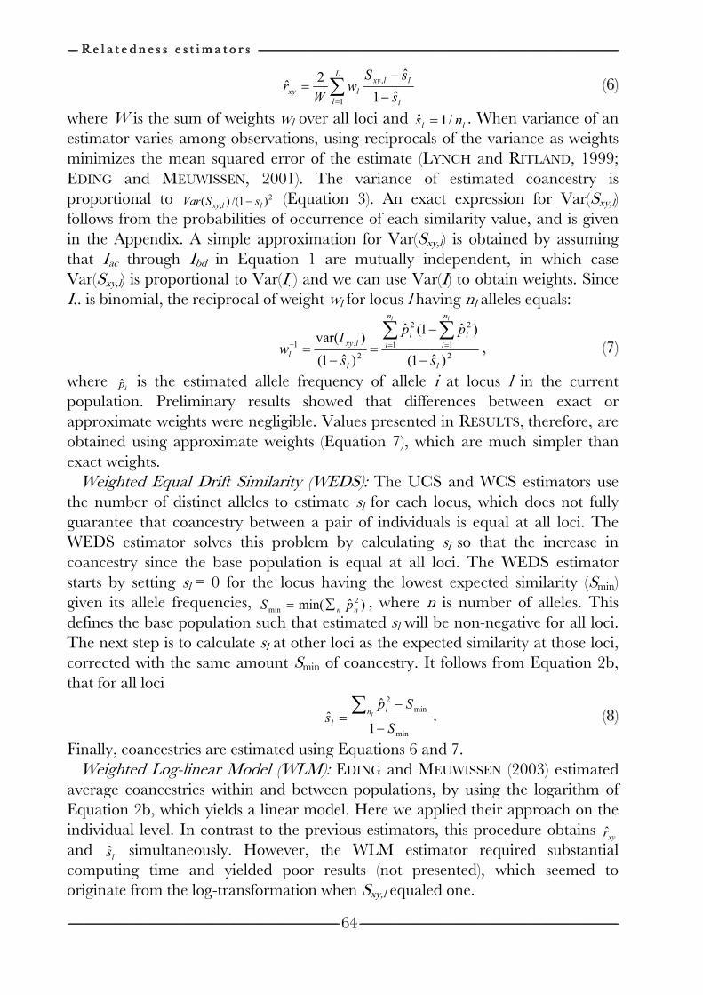
-------------------- R e l a t e d n e s s e s t i m a t o r s R e l a t e d n e s s e s t i m a t o r s R e l a t e d n e s s e s t i m a t o r s R e l a t e d n e s s e s t i m a t o r s --------------------------------------------------------------------------------------------------------------------------------------------------------------------------------------------------------------------------------------------------------------------------------------------------------------------------------------------------------------------------------------------------------------------------------------------------------------------------------------------------------------------------------------------------------------------------------------------------------------------------------------------------------------------------------------------------------------------------------------------------------------------------------------------------------------------------------------------------------
-------------------------------------------------------------------------------------------------------------------------------------------------------------------------------------------------------------------------------------------------------------------------------------------------------------------------------------------------------------------------------------------------------------------------------------------------------------------------------------------------------------------------------------------------------------------------------------------------------------------------------------------- ----------------------------------------------------------------------------------------------------------------------------------------------------------------------------------------------------------------------------------------------------------------------------------------------------------------------------------------------------------------------------------------------------------------------------------------------------------------------------------------------------------------------------------------------------------------------------------------------------------------
64
∑= −
−=
L
l l
llxy
lxys
sSw
Wr
1
,
ˆ1
ˆ2ˆ ((66))
where W is the sum of weights wl over all loci and ll ns /1ˆ = . When variance of an
estimator varies among observations, using reciprocals of the variance as weights minimizes the mean squared error of the estimate (LYNCH and RITLAND, 1999; EDING and MEUWISSEN, 2001). The variance of estimated coancestry is proportional to 2
, )1/()( llxy sSVar − (Equation 3). An exact expression for Var(Sxy,l) follows from the probabilities of occurrence of each similarity value, and is given in the Appendix. A simple approximation for Var(Sxy,l) is obtained by assuming that Iac through Ibd in Equation 1 are mutually independent, in which case Var(Sxy,l) is proportional to Var(I..) and we can use Var(I) to obtain weights. Since I.. is binomial, the reciprocal of weight wl for locus l having nl alleles equals:
2
1
2
1
2
2
,1
)ˆ1(
)ˆ1(ˆ
)ˆ1(
)var(
l
n
i
i
n
i
i
l
lxy
ls
pp
s
Iw
ll
−
−
=−
=∑∑==− ,, ((77))
where ip is the estimated allele frequency of allele i at locus l in the current
population. Preliminary results showed that differences between exact or approximate weights were negligible. Values presented in RESULTS, therefore, are obtained using approximate weights (Equation 7), which are much simpler than exact weights.
Weighted Equal Drift Similarity (WEDS): The UCS and WCS estimators use the number of distinct alleles to estimate sl for each locus, which does not fully guarantee that coancestry between a pair of individuals is equal at all loci. The WEDS estimator solves this problem by calculating sl so that the increase in coancestry since the base population is equal at all loci. The WEDS estimator starts by setting sl = 0 for the locus having the lowest expected similarity (Smin) given its allele frequencies, )ˆmin( 2
min nn pS ∑= , where n is number of alleles. This defines the base population such that estimated sl will be non-negative for all loci. The next step is to calculate sl at other loci as the expected similarity at those loci, corrected with the same amount Smin of coancestry. It follows from Equation 2b, that for all loci
min
min
2
1
ˆˆ
S
Sps ln
i
l−
−=∑
.. ((88))
Finally, coancestries are estimated using Equations 6 and 7. Weighted Log-linear Model (WLM): EDING and MEUWISSEN (2003) estimated
average coancestries within and between populations, by using the logarithm of Equation 2b, which yields a linear model. Here we applied their approach on the individual level. In contrast to the previous estimators, this procedure obtains
xyr and
ls simultaneously. However, the WLM estimator required substantial computing time and yielded poor results (not presented), which seemed to originate from the log-transformation when Sxy,l equaled one.
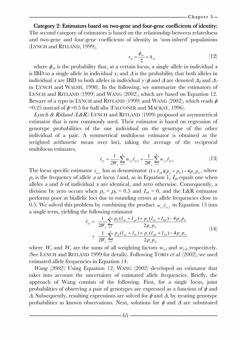
------------------------------------------------------------------------------------------------------------------------------------------------------------------------------------------------------------------------------------------------------------------------------------------------------------------------------------------------------------------------------------------------------------------------------------------------------------------------------------------------------------------------------------------------------------------------------------------------------------------------------------------------------------------------------------------------------------------------------------------------------------------------------------------------------------------------------------------------------------------------------------------------------------------------------------------------------------------------------------------------------------------------------------------------------------------------------------------------ C h a p t e r C h a p t e r C h a p t e r C h a p t e r 5555 --------------------
---------------------------------------------------------------------------------------------------------------------------------------------------------------------------------------------------------------------------------------------------------------------------------------------------------------------------------------------------------------------------------------------------------------------------------------------------------------------------------------------------------------------------------------------------------------------------------------------------------------------------------------- --------------------------------------------------------------------------------------------------------------------------------------------------------------------------------------------------------------------------------------------------------------------------------------------------------------------------------------------------------------------------------------------------------------------------------------------------------------------------------------------------------------------------------------------------------------------------------------------------------
65
Category 2: Estimators based on twoCategory 2: Estimators based on twoCategory 2: Estimators based on twoCategory 2: Estimators based on two----gene and fourgene and fourgene and fourgene and four----gene cgene cgene cgene coefficients of identity: oefficients of identity: oefficients of identity: oefficients of identity: The second category of estimators is based on the relationship between relatedness and two-gene and four-gene coefficients of identity in ‘non-inbred’ populations (LYNCH and RITLAND, 1999),
xy
xy
xyr ∆+=2
φ ((1122))
where φxy is the probability that, at a certain locus, a single allele in individual x is IBD to a single allele in individual y, and ∆ is the probability that both alleles in individual x are IBD to both alleles in individual y (φ and ∆ are denoted ∆8 and ∆7 in LYNCH and WALSH, 1998). In the following, we summarize the estimators of LYNCH and RITLAND (1999) and WANG (2002), which are based on Equation 12. Beware of a typo in LYNCH and RITLAND (1999) and WANG (2002), which reads φ =0.25 instead of φ =0.5 for half sibs (FALCONER and MACKAY, 1996).
Lynch & Ritland (L&R): LYNCH and RITLAND (1999) proposed an asymmetrical estimator that is now commonly used. Their estimator is based on regression of genotype probabilities of the one individual on the genotype of the other individual of a pair. A symmetrical multilocus estimator is obtained as the weighted arithmetic mean over loci, taking the average of the reciprocal multilocus estimates,
lyx
L
l
ly
y
lxy
L
l
lx
x
xy rwW
rwW
r ,
1
,,
1
,ˆ
2
1ˆ
2
1ˆ ∑∑
==
+= ((1133))
The locus specific estimator lxyr ,
ˆ has as denominator babaab ppppI 4))(1( −++ , where
pa is the frequency of allele a at locus l and, as in Equation 1, Iab equals one when alleles a and b of individual x are identical, and zero otherwise. Consequently, a division by zero occurs when pa = pb = 0.5 and Iab = 0, and the L&R estimator performs poor at biallelic loci due to rounding errors at allele frequencies close to 0.5. We solved this problem by combining the product
lxylx rw ,.ˆ in Equation 13 into
a single term, yielding the following estimator
∑
∑
=
=
−++++
−+++=
L
l dc
dcbdadcbcacd
y
L
l ba
babdbcaadacb
x
xy
pp
ppIIpIIp
W
pp
ppIIpIIp
Wr
1
1
2
4)()(
2
1
2
4)()(
2
1ˆ
((1144))
where Wx and Wy are the sums of all weighting factors wx,l and wy,l, respectively. (See LYNCH and RITLAND 1999 for details). Following TORO et al. (2002), we used estimated allele frequencies in Equation 14.
Wang (2002): Using Equation 12, WANG (2002) developed an estimator that takes into account the uncertainty of estimated allele frequencies. Briefly, the approach of Wang consists of the following. First, for a single locus, joint probabilities of observing a pair of genotypes are expressed as a function of φ and ∆. Subsequently, resulting expressions are solved for φ and ∆, by treating genotype probabilities as known observations. Next, solutions for φ and ∆ are substituted
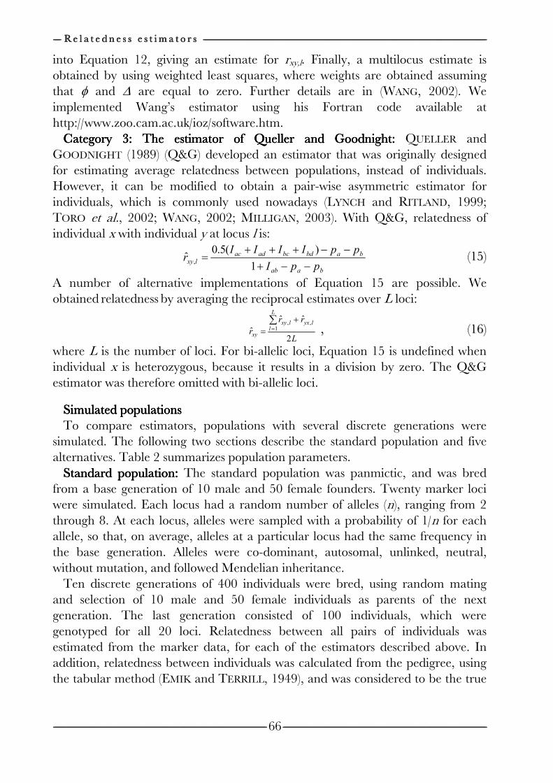
-------------------- R e l a t e d n e s s e s t i m a t o r s R e l a t e d n e s s e s t i m a t o r s R e l a t e d n e s s e s t i m a t o r s R e l a t e d n e s s e s t i m a t o r s --------------------------------------------------------------------------------------------------------------------------------------------------------------------------------------------------------------------------------------------------------------------------------------------------------------------------------------------------------------------------------------------------------------------------------------------------------------------------------------------------------------------------------------------------------------------------------------------------------------------------------------------------------------------------------------------------------------------------------------------------------------------------------------------------------------------------------------------------------
-------------------------------------------------------------------------------------------------------------------------------------------------------------------------------------------------------------------------------------------------------------------------------------------------------------------------------------------------------------------------------------------------------------------------------------------------------------------------------------------------------------------------------------------------------------------------------------------------------------------------------------------- ----------------------------------------------------------------------------------------------------------------------------------------------------------------------------------------------------------------------------------------------------------------------------------------------------------------------------------------------------------------------------------------------------------------------------------------------------------------------------------------------------------------------------------------------------------------------------------------------------------------
66
into Equation 12, giving an estimate for rxy,l. Finally, a multilocus estimate is obtained by using weighted least squares, where weights are obtained assuming that φ and ∆ are equal to zero. Further details are in (WANG, 2002). We implemented Wang’s estimator using his Fortran code available at http://www.zoo.cam.ac.uk/ioz/software.htm.
Category 3: The estimator of Queller and GoodCategory 3: The estimator of Queller and GoodCategory 3: The estimator of Queller and GoodCategory 3: The estimator of Queller and Goodnight: night: night: night: QUELLER and GOODNIGHT (1989) (Q&G) developed an estimator that was originally designed for estimating average relatedness between populations, instead of individuals. However, it can be modified to obtain a pair-wise asymmetric estimator for individuals, which is commonly used nowadays (LYNCH and RITLAND, 1999; TORO et al., 2002; WANG, 2002; MILLIGAN, 2003). With Q&G, relatedness of individual x with individual y at locus l is:
baab
babdbcadaclxy
ppI
ppIIIIr
−−+
−−+++=
1
)(5.0ˆ, ((1155))
A number of alternative implementations of Equation 15 are possible. We obtained relatedness by averaging the reciprocal estimates over L loci:
L
rr
r
L
llyxlxy
xy2
ˆˆ
ˆ 1,,∑
=
+
= ,, ((1166))
where L is the number of loci. For bi-allelic loci, Equation 15 is undefined when individual x is heterozygous, because it results in a division by zero. The Q&G estimator was therefore omitted with bi-allelic loci.
Simulated populationsSimulated populationsSimulated populationsSimulated populations To compare estimators, populations with several discrete generations were
simulated. The following two sections describe the standard population and five alternatives. Table 2 summarizes population parameters.
Standard population: Standard population: Standard population: Standard population: The standard population was panmictic, and was bred from a base generation of 10 male and 50 female founders. Twenty marker loci were simulated. Each locus had a random number of alleles (n), ranging from 2 through 8. At each locus, alleles were sampled with a probability of 1/n for each allele, so that, on average, alleles at a particular locus had the same frequency in the base generation. Alleles were co-dominant, autosomal, unlinked, neutral, without mutation, and followed Mendelian inheritance.
Ten discrete generations of 400 individuals were bred, using random mating and selection of 10 male and 50 female individuals as parents of the next generation. The last generation consisted of 100 individuals, which were genotyped for all 20 loci. Relatedness between all pairs of individuals was estimated from the marker data, for each of the estimators described above. In addition, relatedness between individuals was calculated from the pedigree, using the tabular method (EMIK and TERRILL, 1949), and was considered to be the true
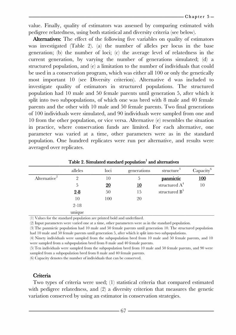
------------------------------------------------------------------------------------------------------------------------------------------------------------------------------------------------------------------------------------------------------------------------------------------------------------------------------------------------------------------------------------------------------------------------------------------------------------------------------------------------------------------------------------------------------------------------------------------------------------------------------------------------------------------------------------------------------------------------------------------------------------------------------------------------------------------------------------------------------------------------------------------------------------------------------------------------------------------------------------------------------------------------------------------------------------------------------------------------ C h a p t e r C h a p t e r C h a p t e r C h a p t e r 5555 --------------------
---------------------------------------------------------------------------------------------------------------------------------------------------------------------------------------------------------------------------------------------------------------------------------------------------------------------------------------------------------------------------------------------------------------------------------------------------------------------------------------------------------------------------------------------------------------------------------------------------------------------------------------- --------------------------------------------------------------------------------------------------------------------------------------------------------------------------------------------------------------------------------------------------------------------------------------------------------------------------------------------------------------------------------------------------------------------------------------------------------------------------------------------------------------------------------------------------------------------------------------------------------
67
value. Finally, quality of estimators was assessed by comparing estimated with pedigree relatedness, using both statistical and diversity criteria (see below).
Alternatives: Alternatives: Alternatives: Alternatives: The effect of the following five variables on quality of estimators was investigated (Table 2). (a) the number of alleles per locus in the base generation; (b) the number of loci; (c) the average level of relatedness in the current generation, by varying the number of generations simulated; (d) a structured population, and (e) a limitation to the number of individuals that could be used in a conservation program, which was either all 100 or only the genetically most important 10 (see Diversity criterion). Alternative d was included to investigate quality of estimators in structured populations. The structured population had 10 male and 50 female parents until generation 5, after which it split into two subpopulations, of which one was bred with 8 male and 40 female parents and the other with 10 male and 50 female parents. Two final generations of 100 individuals were simulated, and 90 individuals were sampled from one and 10 from the other population, or vice versa. Alternative (e) resembles the situation in practice, where conservation funds are limited. For each alternative, one parameter was varied at a time, other parameters were as in the standard population. One hundred replicates were run per alternative, and results were averaged over replicates.
Table 2. Simulated standard populationTable 2. Simulated standard populationTable 2. Simulated standard populationTable 2. Simulated standard population1111 and alternativesand alternativesand alternativesand alternatives
alleles loci generations structure3 Capacity6
Alternative2 2 10 5 panmicticpanmicticpanmicticpanmictic 100100100100
5 20202020 10101010 structured A4 10
2222----8888 50 15 structured B5
10 100 20
2-18
unique (1) Values for the standard population are printed bold and underlined. (2) Input parameters were varied one at a time, other parameters were as in the standard population. (3) The panmictic population had 10 male and 50 female parents until generation 10. The structured population had 10 male and 50 female parents until generation 5, after which it split into two subpopulations. (4) Ninety individuals were sampled from the subpopulation bred from 10 male and 50 female parents, and 10 were sampled from a subpopulation bred from 8 male and 40 female parents. (5) Ten individuals were sampled from the subpopulation bred from 10 male and 50 female parents, and 90 were sampled from a subpopulation bred from 8 male and 40 female parents. (6) Capacity denotes the number of individuals that can be conserved.
CriteriaCriteriaCriteriaCriteria Two types of criteria were used; (1) statistical criteria that compared estimated
with pedigree relatedness, and (2) a diversity criterion that measures the genetic variation conserved by using an estimator in conservation strategies.
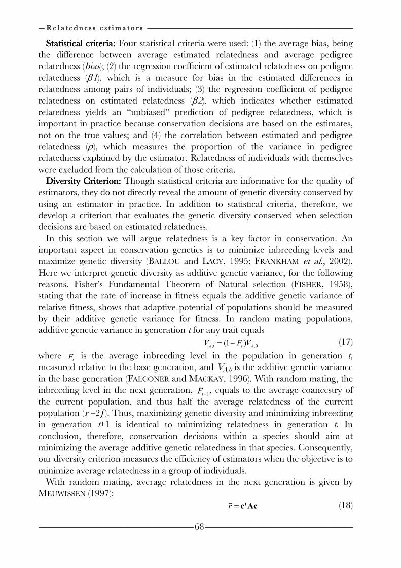
-------------------- R e l a t e d n e s s e s t i m a t o r s R e l a t e d n e s s e s t i m a t o r s R e l a t e d n e s s e s t i m a t o r s R e l a t e d n e s s e s t i m a t o r s --------------------------------------------------------------------------------------------------------------------------------------------------------------------------------------------------------------------------------------------------------------------------------------------------------------------------------------------------------------------------------------------------------------------------------------------------------------------------------------------------------------------------------------------------------------------------------------------------------------------------------------------------------------------------------------------------------------------------------------------------------------------------------------------------------------------------------------------------------
-------------------------------------------------------------------------------------------------------------------------------------------------------------------------------------------------------------------------------------------------------------------------------------------------------------------------------------------------------------------------------------------------------------------------------------------------------------------------------------------------------------------------------------------------------------------------------------------------------------------------------------------- ----------------------------------------------------------------------------------------------------------------------------------------------------------------------------------------------------------------------------------------------------------------------------------------------------------------------------------------------------------------------------------------------------------------------------------------------------------------------------------------------------------------------------------------------------------------------------------------------------------------
68
Statistical criteria: Statistical criteria: Statistical criteria: Statistical criteria: Four statistical criteria were used: (1) the average bias, being the difference between average estimated relatedness and average pedigree relatedness (bias); (2) the regression coefficient of estimated relatedness on pedigree relatedness (β1), which is a measure for bias in the estimated differences in relatedness among pairs of individuals; (3) the regression coefficient of pedigree relatedness on estimated relatedness (β2), which indicates whether estimated relatedness yields an “unbiased” prediction of pedigree relatedness, which is important in practice because conservation decisions are based on the estimates, not on the true values; and (4) the correlation between estimated and pedigree relatedness (ρ), which measures the proportion of the variance in pedigree relatedness explained by the estimator. Relatedness of individuals with themselves were excluded from the calculation of those criteria.
Diversity Criterion: Diversity Criterion: Diversity Criterion: Diversity Criterion: Though statistical criteria are informative for the quality of estimators, they do not directly reveal the amount of genetic diversity conserved by using an estimator in practice. In addition to statistical criteria, therefore, we develop a criterion that evaluates the genetic diversity conserved when selection decisions are based on estimated relatedness.
In this section we will argue relatedness is a key factor in conservation. An important aspect in conservation genetics is to minimize inbreeding levels and maximize genetic diversity (BALLOU and LACY, 1995; FRANKHAM et al., 2002). Here we interpret genetic diversity as additive genetic variance, for the following reasons. Fisher’s Fundamental Theorem of Natural selection (FISHER, 1958), stating that the rate of increase in fitness equals the additive genetic variance of relative fitness, shows that adaptive potential of populations should be measured by their additive genetic variance for fitness. In random mating populations, additive genetic variance in generation t for any trait equals
0,, )1( AttA VFV −= ((1177))
where tF is the average inbreeding level in the population in generation t,
measured relative to the base generation, and VA,0 is the additive genetic variance in the base generation (FALCONER and MACKAY, 1996). With random mating, the inbreeding level in the next generation,
1+tF , equals to the average coancestry of the current population, and thus half the average relatedness of the current population (r =2ƒ). Thus, maximizing genetic diversity and minimizing inbreeding in generation t+1 is identical to minimizing relatedness in generation t. In conclusion, therefore, conservation decisions within a species should aim at minimizing the average additive genetic relatedness in that species. Consequently, our diversity criterion measures the efficiency of estimators when the objective is to minimize average relatedness in a group of individuals.
With random mating, average relatedness in the next generation is given by MEUWISSEN (1997):
Acc'=r ((1188))
------------------------------------------------------------------------------------------------------------------------------------------------------------------------------------------------------------------------------------------------------------------------------------------------------------------------------------------------------------------------------------------------------------------------------------------------------------------------------------------------------------------------------------------------------------------------------------------------------------------------------------------------------------------------------------------------------------------------------------------------------------------------------------------------------------------------------------------------------------------------------------------------------------------------------------------------------------------------------------------------------------------------------------------------------------------------------------------------ C h a p t e r C h a p t e r C h a p t e r C h a p t e r 5555 --------------------
---------------------------------------------------------------------------------------------------------------------------------------------------------------------------------------------------------------------------------------------------------------------------------------------------------------------------------------------------------------------------------------------------------------------------------------------------------------------------------------------------------------------------------------------------------------------------------------------------------------------------------------- --------------------------------------------------------------------------------------------------------------------------------------------------------------------------------------------------------------------------------------------------------------------------------------------------------------------------------------------------------------------------------------------------------------------------------------------------------------------------------------------------------------------------------------------------------------------------------------------------------
69
where cccc is a vector of proportional contributions of individuals to the next generation, so that elements of cccc sum to one, and AAAA is a matrix of additive genetic relatedness between all individuals, including relatedness of individuals with themselves. Average relatedness among parents, and thus the inbreeding level in the next generation, can be decreased or increased by varying the contributions of individuals (cccc). Thus average relatedness can be minimized by finding an optimum contribution vector
oc that minimizes cccc’’’’AcAcAcAc, which is given by MEUWISSEN (1997) and EDING et al. (2002):
1A1'
1Ac
1
1
o −
−
= ((1199))
where 1111 is a column vector of one’s. The matrix of additive genetic relationships has to be estimated from marker data. The amount of genetic diversity conserved by using estimated optimal contributions (
oc ) will depend on the estimator used. To obtain estimated optimum contributions, we substituted the matrix of pedigree relatedness by the matrix of estimated relatedness ( A ) in Equation 19. When negative contributions were obtained, the most negative contribution was set to zero and optimal contributions were recalculated, until all contributions were non-negative. In alternative (e) the lowest contribution was set to zero and optimal contributions were recalculated, until all contributions were non-negative or only 10 contributions were left.
We evaluated the result on two scales. On the first scale, the diversity criterion equals the proportion of additive genetic variance conserved relative to the base generation,
oocA'c ˆˆ1
21−=eH ((2200))
which is derived by combining equations 17 and 18. Note that, in Equation 20, AAAA refers to relatedness calculated from the pedigree. With random mating, He equals expected heterozygosity in a population with estimated optimum contributions of individuals, expressed as a proportion of heterozygosity in the base generation. On the second scale, the diversity criterion equals the number of founders (Nge) that would have the same average coancestry (and thus the same additive genetic variance) as the population obtained using estimated optimum contributions. Average coancestry among N founders equals 1/(2N), so that Nge equals
oo cA'c ˆˆ
1=ge� ((2211))
CABALLERO and TORO (2000) referred to Nge as the number of founder genome equivalents. Equation 21 is an expression on the scale of effective population size, since it equals )2/(1 f� ge = .
In contrast to the statistical criteria, relatedness of individuals with themselves were included in A , and were estimated by using y = x in the relevant expressions for
xyr .
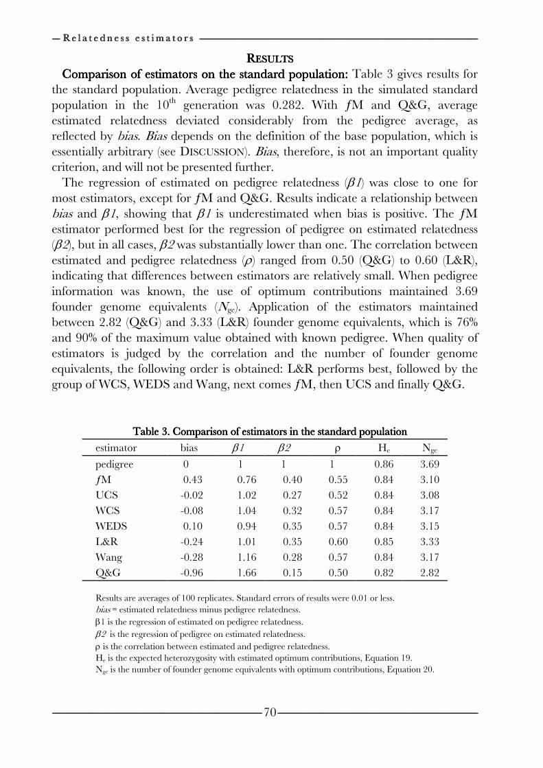
-------------------- R e l a t e d n e s s e s t i m a t o r s R e l a t e d n e s s e s t i m a t o r s R e l a t e d n e s s e s t i m a t o r s R e l a t e d n e s s e s t i m a t o r s --------------------------------------------------------------------------------------------------------------------------------------------------------------------------------------------------------------------------------------------------------------------------------------------------------------------------------------------------------------------------------------------------------------------------------------------------------------------------------------------------------------------------------------------------------------------------------------------------------------------------------------------------------------------------------------------------------------------------------------------------------------------------------------------------------------------------------------------------------
-------------------------------------------------------------------------------------------------------------------------------------------------------------------------------------------------------------------------------------------------------------------------------------------------------------------------------------------------------------------------------------------------------------------------------------------------------------------------------------------------------------------------------------------------------------------------------------------------------------------------------------------- ----------------------------------------------------------------------------------------------------------------------------------------------------------------------------------------------------------------------------------------------------------------------------------------------------------------------------------------------------------------------------------------------------------------------------------------------------------------------------------------------------------------------------------------------------------------------------------------------------------------
70
RRRRESULTSESULTSESULTSESULTS Comparison of estimators on the standard poComparison of estimators on the standard poComparison of estimators on the standard poComparison of estimators on the standard population: pulation: pulation: pulation: Table 3 gives results for
the standard population. Average pedigree relatedness in the simulated standard population in the 10th generation was 0.282. With ƒM and Q&G, average estimated relatedness deviated considerably from the pedigree average, as reflected by bias. Bias depends on the definition of the base population, which is essentially arbitrary (see DISCUSSION). Bias, therefore, is not an important quality criterion, and will not be presented further.
The regression of estimated on pedigree relatedness (β1) was close to one for most estimators, except for ƒM and Q&G. Results indicate a relationship between bias and β1, showing that β1 is underestimated when bias is positive. The ƒM estimator performed best for the regression of pedigree on estimated relatedness (β2), but in all cases, β2 was substantially lower than one. The correlation between estimated and pedigree relatedness (ρ) ranged from 0.50 (Q&G) to 0.60 (L&R), indicating that differences between estimators are relatively small. When pedigree information was known, the use of optimum contributions maintained 3.69 founder genome equivalents (Nge). Application of the estimators maintained between 2.82 (Q&G) and 3.33 (L&R) founder genome equivalents, which is 76% and 90% of the maximum value obtained with known pedigree. When quality of estimators is judged by the correlation and the number of founder genome equivalents, the following order is obtained: L&R performs best, followed by the group of WCS, WEDS and Wang, next comes ƒM, then UCS and finally Q&G.
Table 3. Comparison of estimators in the standard population Table 3. Comparison of estimators in the standard population Table 3. Comparison of estimators in the standard population Table 3. Comparison of estimators in the standard population
estimator bias β1 β2 ρ He Nge
pedigree 0 1 1 1 0.86 3.69
ƒM 0.43 0.76 0.40 0.55 0.84 3.10
UCS -0.02 1.02 0.27 0.52 0.84 3.08
WCS -0.08 1.04 0.32 0.57 0.84 3.17
WEDS 0.10 0.94 0.35 0.57 0.84 3.15
L&R -0.24 1.01 0.35 0.60 0.85 3.33
Wang -0.28 1.16 0.28 0.57 0.84 3.17
Q&G -0.96 1.66 0.15 0.50 0.82 2.82 Results are averages of 100 replicates. Standard errors of results were 0.01 or less. bias = estimated relatedness minus pedigree relatedness. β1 is the regression of estimated on pedigree relatedness. β2 is the regression of pedigree on estimated relatedness. ρ is the correlation between estimated and pedigree relatedness. He is the expected heterozygosity with estimated optimum contributions, Equation 19. Nge is the number of founder genome equivalents with optimum contributions, Equation 20.
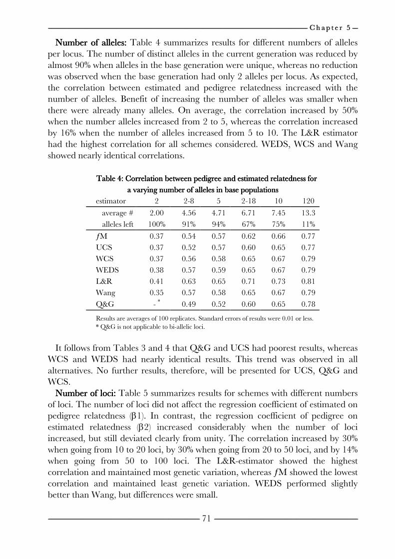
------------------------------------------------------------------------------------------------------------------------------------------------------------------------------------------------------------------------------------------------------------------------------------------------------------------------------------------------------------------------------------------------------------------------------------------------------------------------------------------------------------------------------------------------------------------------------------------------------------------------------------------------------------------------------------------------------------------------------------------------------------------------------------------------------------------------------------------------------------------------------------------------------------------------------------------------------------------------------------------------------------------------------------------------------------------------------------------------ C h a p t e r C h a p t e r C h a p t e r C h a p t e r 5555 --------------------
---------------------------------------------------------------------------------------------------------------------------------------------------------------------------------------------------------------------------------------------------------------------------------------------------------------------------------------------------------------------------------------------------------------------------------------------------------------------------------------------------------------------------------------------------------------------------------------------------------------------------------------- --------------------------------------------------------------------------------------------------------------------------------------------------------------------------------------------------------------------------------------------------------------------------------------------------------------------------------------------------------------------------------------------------------------------------------------------------------------------------------------------------------------------------------------------------------------------------------------------------------
71
Number of alleles: Number of alleles: Number of alleles: Number of alleles: Table 4 summarizes results for different numbers of alleles per locus. The number of distinct alleles in the current generation was reduced by almost 90% when alleles in the base generation were unique, whereas no reduction was observed when the base generation had only 2 alleles per locus. As expected, the correlation between estimated and pedigree relatedness increased with the number of alleles. Benefit of increasing the number of alleles was smaller when there were already many alleles. On average, the correlation increased by 50% when the number alleles increased from 2 to 5, whereas the correlation increased by 16% when the number of alleles increased from 5 to 10. The L&R estimator had the highest correlation for all schemes considered. WEDS, WCS and Wang showed nearly identical correlations.
Table 4: Correlation between pedigree and estimated relatedness for Table 4: Correlation between pedigree and estimated relatedness for Table 4: Correlation between pedigree and estimated relatedness for Table 4: Correlation between pedigree and estimated relatedness for
a varying number of alleles in base populationsa varying number of alleles in base populationsa varying number of alleles in base populationsa varying number of alleles in base populations
estimator 2 2-8 5 2-18 10 120
average #
alleles left
2.00 4.56 4.71 6.71 7.45 13.3
100% 91% 94% 67% 75% 11%
ƒM 0.37 0.54 0.57 0.62 0.66 0.77
UCS 0.37 0.52 0.57 0.60 0.65 0.77
WCS 0.37 0.56 0.58 0.65 0.67 0.79
WEDS 0.38 0.57 0.59 0.65 0.67 0.79
L&R 0.41 0.63 0.65 0.71 0.73 0.81
Wang 0.35 0.57 0.58 0.65 0.67 0.79
Q&G - * 0.49 0.52 0.60 0.65 0.78
Results are averages of 100 replicates. Standard errors of results were 0.01 or less. * Q&G is not applicable to bi-allelic loci.
It follows from Tables 3 and 4 that Q&G and UCS had poorest results, whereas
WCS and WEDS had nearly identical results. This trend was observed in all alternatives. No further results, therefore, will be presented for UCS, Q&G and WCS.
Number of loci:Number of loci:Number of loci:Number of loci: Table 5 summarizes results for schemes with different numbers of loci. The number of loci did not affect the regression coefficient of estimated on pedigree relatedness (β1). In contrast, the regression coefficient of pedigree on estimated relatedness (β2) increased considerably when the number of loci increased, but still deviated clearly from unity. The correlation increased by 30% when going from 10 to 20 loci, by 30% when going from 20 to 50 loci, and by 14% when going from 50 to 100 loci. The L&R-estimator showed the highest correlation and maintained most genetic variation, whereas ƒM showed the lowest correlation and maintained least genetic variation. WEDS performed slightly better than Wang, but differences were small.
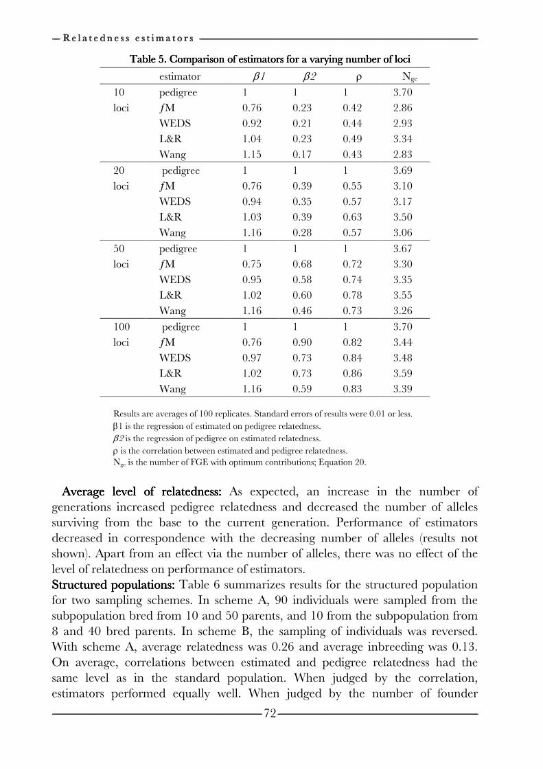
-------------------- R e l a t e d n e s s e s t i m a t o r s R e l a t e d n e s s e s t i m a t o r s R e l a t e d n e s s e s t i m a t o r s R e l a t e d n e s s e s t i m a t o r s --------------------------------------------------------------------------------------------------------------------------------------------------------------------------------------------------------------------------------------------------------------------------------------------------------------------------------------------------------------------------------------------------------------------------------------------------------------------------------------------------------------------------------------------------------------------------------------------------------------------------------------------------------------------------------------------------------------------------------------------------------------------------------------------------------------------------------------------------------
-------------------------------------------------------------------------------------------------------------------------------------------------------------------------------------------------------------------------------------------------------------------------------------------------------------------------------------------------------------------------------------------------------------------------------------------------------------------------------------------------------------------------------------------------------------------------------------------------------------------------------------------- ----------------------------------------------------------------------------------------------------------------------------------------------------------------------------------------------------------------------------------------------------------------------------------------------------------------------------------------------------------------------------------------------------------------------------------------------------------------------------------------------------------------------------------------------------------------------------------------------------------------
72
Table 5. Comparison of estimaTable 5. Comparison of estimaTable 5. Comparison of estimaTable 5. Comparison of estimators for a varying number of locitors for a varying number of locitors for a varying number of locitors for a varying number of loci
estimator β1 β2 ρ Nge
10
loci
pedigree 1 1 1 3.70
ƒM 0.76 0.23 0.42 2.86
WEDS 0.92 0.21 0.44 2.93
L&R 1.04 0.23 0.49 3.34
Wang 1.15 0.17 0.43 2.83
20
loci
pedigree 1 1 1 3.69
ƒM 0.76 0.39 0.55 3.10
WEDS 0.94 0.35 0.57 3.17
L&R 1.03 0.39 0.63 3.50
Wang 1.16 0.28 0.57 3.06
50
loci
pedigree 1 1 1 3.67
ƒM 0.75 0.68 0.72 3.30
WEDS 0.95 0.58 0.74 3.35
L&R 1.02 0.60 0.78 3.55
Wang 1.16 0.46 0.73 3.26
100
loci
pedigree 1 1 1 3.70
ƒM 0.76 0.90 0.82 3.44
WEDS 0.97 0.73 0.84 3.48
L&R 1.02 0.73 0.86 3.59
Wang 1.16 0.59 0.83 3.39 Results are averages of 100 replicates. Standard errors of results were 0.01 or less. β1 is the regression of estimated on pedigree relatedness. β2 is the regression of pedigree on estimated relatedness. ρ is the correlation between estimated and pedigree relatedness. Nge is the number of FGE with optimum contributions; Equation 20.
Average level of relatedness:Average level of relatedness:Average level of relatedness:Average level of relatedness: As expected, an increase in the number of generations increased pedigree relatedness and decreased the number of alleles surviving from the base to the current generation. Performance of estimators decreased in correspondence with the decreasing number of alleles (results not shown). Apart from an effect via the number of alleles, there was no effect of the level of relatedness on performance of estimators. Structured populations:Structured populations:Structured populations:Structured populations: Table 6 summarizes results for the structured population for two sampling schemes. In scheme A, 90 individuals were sampled from the subpopulation bred from 10 and 50 parents, and 10 from the subpopulation from 8 and 40 bred parents. In scheme B, the sampling of individuals was reversed. With scheme A, average relatedness was 0.26 and average inbreeding was 0.13. On average, correlations between estimated and pedigree relatedness had the same level as in the standard population. When judged by the correlation, estimators performed equally well. When judged by the number of founder
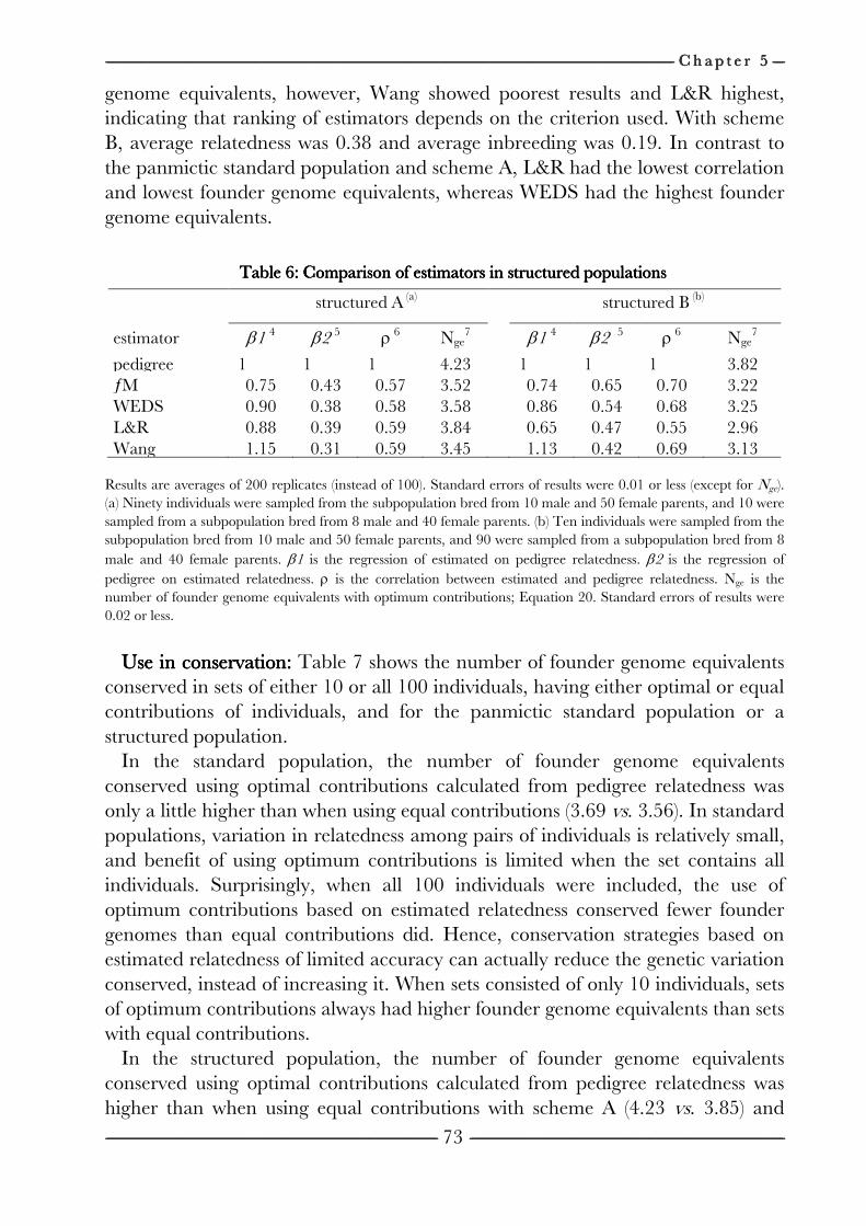
------------------------------------------------------------------------------------------------------------------------------------------------------------------------------------------------------------------------------------------------------------------------------------------------------------------------------------------------------------------------------------------------------------------------------------------------------------------------------------------------------------------------------------------------------------------------------------------------------------------------------------------------------------------------------------------------------------------------------------------------------------------------------------------------------------------------------------------------------------------------------------------------------------------------------------------------------------------------------------------------------------------------------------------------------------------------------------------------ C h a p t e r C h a p t e r C h a p t e r C h a p t e r 5555 --------------------
---------------------------------------------------------------------------------------------------------------------------------------------------------------------------------------------------------------------------------------------------------------------------------------------------------------------------------------------------------------------------------------------------------------------------------------------------------------------------------------------------------------------------------------------------------------------------------------------------------------------------------------- --------------------------------------------------------------------------------------------------------------------------------------------------------------------------------------------------------------------------------------------------------------------------------------------------------------------------------------------------------------------------------------------------------------------------------------------------------------------------------------------------------------------------------------------------------------------------------------------------------
73
genome equivalents, however, Wang showed poorest results and L&R highest, indicating that ranking of estimators depends on the criterion used. With scheme B, average relatedness was 0.38 and average inbreeding was 0.19. In contrast to the panmictic standard population and scheme A, L&R had the lowest correlation and lowest founder genome equivalents, whereas WEDS had the highest founder genome equivalents.
Table 6: Comparison of Table 6: Comparison of Table 6: Comparison of Table 6: Comparison of estimators in structured populatioestimators in structured populatioestimators in structured populatioestimators in structured populationsnsnsns
structured A (a) structured B (b)
estimator β1 4 β2 5 ρ 6 Nge7 β1 4 β2 5 ρ 6 Nge
7
pedigree 1 1 1 4.23 1 1 1 3.82 ƒM 0.75 0.43 0.57 3.52 0.74 0.65 0.70 3.22 WEDS 0.90 0.38 0.58 3.58 0.86 0.54 0.68 3.25 L&R 0.88 0.39 0.59 3.84 0.65 0.47 0.55 2.96 Wang 1.15 0.31 0.59 3.45 1.13 0.42 0.69 3.13
Results are averages of 200 replicates (instead of 100). Standard errors of results were 0.01 or less (except for Nge). (a) Ninety individuals were sampled from the subpopulation bred from 10 male and 50 female parents, and 10 were sampled from a subpopulation bred from 8 male and 40 female parents. (b) Ten individuals were sampled from the subpopulation bred from 10 male and 50 female parents, and 90 were sampled from a subpopulation bred from 8 male and 40 female parents. β1 is the regression of estimated on pedigree relatedness. β2 is the regression of pedigree on estimated relatedness. ρ is the correlation between estimated and pedigree relatedness. Nge is the number of founder genome equivalents with optimum contributions; Equation 20. Standard errors of results were 0.02 or less.
Use in conservation: Use in conservation: Use in conservation: Use in conservation: Table 7 shows the number of founder genome equivalents
conserved in sets of either 10 or all 100 individuals, having either optimal or equal contributions of individuals, and for the panmictic standard population or a structured population.
In the standard population, the number of founder genome equivalents conserved using optimal contributions calculated from pedigree relatedness was only a little higher than when using equal contributions (3.69 vs. 3.56). In standard populations, variation in relatedness among pairs of individuals is relatively small, and benefit of using optimum contributions is limited when the set contains all individuals. Surprisingly, when all 100 individuals were included, the use of optimum contributions based on estimated relatedness conserved fewer founder genomes than equal contributions did. Hence, conservation strategies based on estimated relatedness of limited accuracy can actually reduce the genetic variation conserved, instead of increasing it. When sets consisted of only 10 individuals, sets of optimum contributions always had higher founder genome equivalents than sets with equal contributions.
In the structured population, the number of founder genome equivalents conserved using optimal contributions calculated from pedigree relatedness was higher than when using equal contributions with scheme A (4.23 vs. 3.85) and
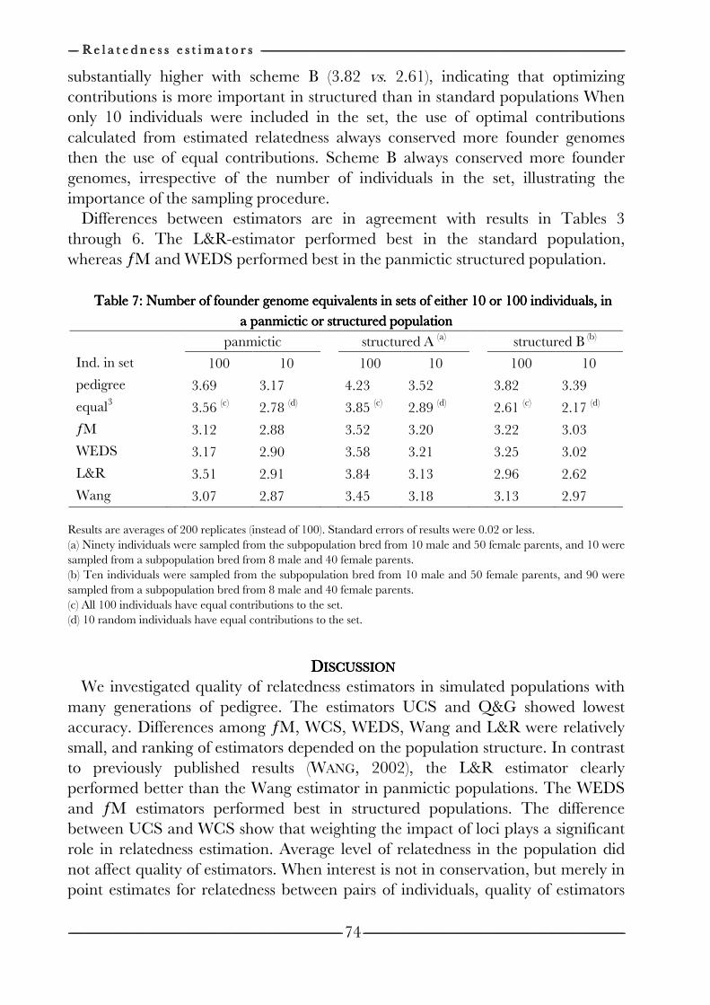
-------------------- R e l a t e d n e s s e s t i m a t o r s R e l a t e d n e s s e s t i m a t o r s R e l a t e d n e s s e s t i m a t o r s R e l a t e d n e s s e s t i m a t o r s --------------------------------------------------------------------------------------------------------------------------------------------------------------------------------------------------------------------------------------------------------------------------------------------------------------------------------------------------------------------------------------------------------------------------------------------------------------------------------------------------------------------------------------------------------------------------------------------------------------------------------------------------------------------------------------------------------------------------------------------------------------------------------------------------------------------------------------------------------
-------------------------------------------------------------------------------------------------------------------------------------------------------------------------------------------------------------------------------------------------------------------------------------------------------------------------------------------------------------------------------------------------------------------------------------------------------------------------------------------------------------------------------------------------------------------------------------------------------------------------------------------- ----------------------------------------------------------------------------------------------------------------------------------------------------------------------------------------------------------------------------------------------------------------------------------------------------------------------------------------------------------------------------------------------------------------------------------------------------------------------------------------------------------------------------------------------------------------------------------------------------------------
74
substantially higher with scheme B (3.82 vs. 2.61), indicating that optimizing contributions is more important in structured than in standard populations When only 10 individuals were included in the set, the use of optimal contributions calculated from estimated relatedness always conserved more founder genomes then the use of equal contributions. Scheme B always conserved more founder genomes, irrespective of the number of individuals in the set, illustrating the importance of the sampling procedure.
Differences between estimators are in agreement with results in Tables 3 through 6. The L&R-estimator performed best in the standard population, whereas ƒM and WEDS performed best in the panmictic structured population.
Table 7: Number of founder genome equivTable 7: Number of founder genome equivTable 7: Number of founder genome equivTable 7: Number of founder genome equivalents in sets of either 10 or 100 individuals, in alents in sets of either 10 or 100 individuals, in alents in sets of either 10 or 100 individuals, in alents in sets of either 10 or 100 individuals, in
a panmictic or structured populationa panmictic or structured populationa panmictic or structured populationa panmictic or structured population panmictic structured A (a) structured B (b)
Ind. in set 100 10 100 10 100 10
pedigree 3.69 3.17 4.23 3.52 3.82 3.39
equal3 3.56 (c) 2.78 (d) 3.85 (c) 2.89 (d) 2.61 (c) 2.17 (d)
ƒM 3.12 2.88 3.52 3.20 3.22 3.03
WEDS 3.17 2.90 3.58 3.21 3.25 3.02
L&R 3.51 2.91 3.84 3.13 2.96 2.62
Wang 3.07 2.87 3.45 3.18 3.13 2.97
Results are averages of 200 replicates (instead of 100). Standard errors of results were 0.02 or less. (a) Ninety individuals were sampled from the subpopulation bred from 10 male and 50 female parents, and 10 were sampled from a subpopulation bred from 8 male and 40 female parents. (b) Ten individuals were sampled from the subpopulation bred from 10 male and 50 female parents, and 90 were sampled from a subpopulation bred from 8 male and 40 female parents. (c) All 100 individuals have equal contributions to the set. (d) 10 random individuals have equal contributions to the set.
DDDDISCUSSIONISCUSSIONISCUSSIONISCUSSION We investigated quality of relatedness estimators in simulated populations with
many generations of pedigree. The estimators UCS and Q&G showed lowest accuracy. Differences among ƒM, WCS, WEDS, Wang and L&R were relatively small, and ranking of estimators depended on the population structure. In contrast to previously published results (WANG, 2002), the L&R estimator clearly performed better than the Wang estimator in panmictic populations. The WEDS and ƒM estimators performed best in structured populations. The difference between UCS and WCS show that weighting the impact of loci plays a significant role in relatedness estimation. Average level of relatedness in the population did not affect quality of estimators. When interest is not in conservation, but merely in point estimates for relatedness between pairs of individuals, quality of estimators
------------------------------------------------------------------------------------------------------------------------------------------------------------------------------------------------------------------------------------------------------------------------------------------------------------------------------------------------------------------------------------------------------------------------------------------------------------------------------------------------------------------------------------------------------------------------------------------------------------------------------------------------------------------------------------------------------------------------------------------------------------------------------------------------------------------------------------------------------------------------------------------------------------------------------------------------------------------------------------------------------------------------------------------------------------------------------------------------ C h a p t e r C h a p t e r C h a p t e r C h a p t e r 5555 --------------------
---------------------------------------------------------------------------------------------------------------------------------------------------------------------------------------------------------------------------------------------------------------------------------------------------------------------------------------------------------------------------------------------------------------------------------------------------------------------------------------------------------------------------------------------------------------------------------------------------------------------------------------- --------------------------------------------------------------------------------------------------------------------------------------------------------------------------------------------------------------------------------------------------------------------------------------------------------------------------------------------------------------------------------------------------------------------------------------------------------------------------------------------------------------------------------------------------------------------------------------------------------
75
may be judged by the correlation between true and estimated relatedness. When judged by the correlation, L&R performs best in panmictic populations and WEDS, ƒM and Wang in structured populations. FERNANDEZ et al. (2005) argued that minimizing simple molecular coancestry (ƒM) is the optimum way to maximize diversity, which would imply that other relatedness estimators are redundant. Our results show, however, that there is clear benefit of using more sophisticated relatedness estimators (see e.g. L&R vs. ƒM in Table 5). In structured populations, sets of estimated optimum contributions had in most cases more diversity than sets of equal contributions of individuals. Surprisingly, in panmictic populations, sets of optimum estimated contributions sometimes had less diversity than sets with equal contributions of individuals, showing that estimates of relatedness can be useful in conservation programs, but should be used with caution.
L&R versus Wang:L&R versus Wang:L&R versus Wang:L&R versus Wang: In contrast to results presented by WANG (2002), the L&R-estimator performed consistently better than the Wang-estimator in panmictic populations, irrespective of the numbers of alleles and loci. We identified three reasons for this discrepancy. (1) We have used a modified version of the L&R estimator which avoids the numerical rounding errors which may occur when pa = pb = 0.5 or when estimates “blow up” when they approach this value. WANG (2002) noted this problem, but did not correct for it. We observed that the L&R-estimator improved considerably when calculating the product of relatedness and weight in a single step (Equation 14). However, with the exception of bi-allelic loci, L&R also performed better than Wang when relatedness and the weight were calculated separately, indicating that this cannot be the only source of differences. (2) WANG (2002) presented results only for close relatives of a single type at a time, either non-relatives, full sibs or half sibs. In reality, however, pedigree relatedness is unknown so that it is impossible to a priori distinguish between different types of relatives. Pedigree relatedness will take many distinct values, since all real populations have many generations of pedigree. It is not possible, therefore, to judge performance of the Wang-estimator in general populations from results presented in WANG (2002). In the present study, we considered populations with general relationships and evaluated estimators by the correlation between pedigree and estimated relatedness, without a priori distinguishing between categories of relatives. (3) WANG (2002) observed that the L&R-estimator performed better for “unrelated” individuals (i.e. not sibs or parent-offspring), which will be the majority even in small populations. In contrast to current belief, therefore, we find the L&R-estimator to be superior to the Wang-estimator in panmictic populations. Furthermore, the L&R-estimator is substantially simpler.
Bias and base population:Bias and base population:Bias and base population:Bias and base population: For most estimators, average estimated relatedness differed substantially from average pedigree relatedness, but the difference (bias) was unrelated to the accuracy (ρ) of estimators, illustrating that the choice of a
-------------------- R e l a t e d n e s s e s t i m a t o r s R e l a t e d n e s s e s t i m a t o r s R e l a t e d n e s s e s t i m a t o r s R e l a t e d n e s s e s t i m a t o r s --------------------------------------------------------------------------------------------------------------------------------------------------------------------------------------------------------------------------------------------------------------------------------------------------------------------------------------------------------------------------------------------------------------------------------------------------------------------------------------------------------------------------------------------------------------------------------------------------------------------------------------------------------------------------------------------------------------------------------------------------------------------------------------------------------------------------------------------------------
-------------------------------------------------------------------------------------------------------------------------------------------------------------------------------------------------------------------------------------------------------------------------------------------------------------------------------------------------------------------------------------------------------------------------------------------------------------------------------------------------------------------------------------------------------------------------------------------------------------------------------------------- ----------------------------------------------------------------------------------------------------------------------------------------------------------------------------------------------------------------------------------------------------------------------------------------------------------------------------------------------------------------------------------------------------------------------------------------------------------------------------------------------------------------------------------------------------------------------------------------------------------------
76
base population is arbitrary in a panmictic population. Bias depends on the way estimators define the base population or, in other words, how they divide the average observed similarity into a proportion due to IBD vs. a proportion due to AIS. The L&R and Wang estimators set the probability of AIS equal to the expected homozygosity in the current population, which implicitly defines the current generation as base population. Average estimated relatedness is therefore close to zero for Wang and L&R, bias is negative, and many estimates are negative. Negative estimates may seem confusing, because relatedness equals twice the probability that alleles are IBD, which cannot be negative by definition. However, negative estimates can easily be scaled to positive values using an equation similar to Equation 8, which solves the interpretation problem (see also EDING and MEUWISSEN 2003). Alternatively, relatedness may be interpreted as a measure of additive genetic covariance between individuals, in which case below average values indicate individuals with dissimilar breeding values.
Regression of estimated on pedigree relatedness:Regression of estimated on pedigree relatedness:Regression of estimated on pedigree relatedness:Regression of estimated on pedigree relatedness: The regression coefficient of estimated on pedigree relatedness (β1) is a measure of bias. Unbiasedness, i.e.
xyxyxy rrrE =]|ˆ[ , requires that β1 = 1. (Note that the criterion bias refers to average relatedness, whereas β1 refers to pairs of individuals.) There was a clear relationship between bias and β1; positive bias was accompanied by underestimation of β1 (Table 3). This result is due to the population genetic relationship between absolute differences among coancestries of pairs of individuals and the average coancestry level of a population. Equation 3 illustrates this phenomenon. Positive bias, i.e. overestimation of sl, reduces absolute differences between coancestries because similarities are scaled by 1−sl. Alternatively, the relationship can be understood by considering coancestry as a function of generation number (t); t
t ff )1(1 ∆−−= , which is a function starting at zero at t = 0 and asymptoting to 1 when t → ∞ (FALCONER and MACKAY, 1996). At low values of ft the function is steep and differences in coancestries within a generation are large, whereas at high ft the function is flat and differences are small. Thus the relationship between bias and β1 is a direct consequence of standard population genetic theory, and estimators that are consistent with population genetic theory will always show this relationship.
Regression of pedigree on estimated relatedness:Regression of pedigree on estimated relatedness:Regression of pedigree on estimated relatedness:Regression of pedigree on estimated relatedness: The regression coefficient of pedigree on estimated relatedness (β2) may be interpreted as the reciprocal of a usual measure of unbiasedness, i.e. E[[[[rxy r xy]]]]= r xy requires that β2 = 1. (Note that rxy is treated as a random variable here.) In conservation practice, selection of breeding individuals relies on estimated relatedness; pedigree relatedness is unknown. To avoid overestimation of the genetic diversity conserved, it is important that estimated relatedness is an “unbiased” predictor of pedigree relatedness, which requires that β2 equals one. However, β2 = )ˆ(/)ˆ,( rVarrrCov = 1 requires that
rr ρσσ =ˆ , indicating that estimates should have lower variance than
------------------------------------------------------------------------------------------------------------------------------------------------------------------------------------------------------------------------------------------------------------------------------------------------------------------------------------------------------------------------------------------------------------------------------------------------------------------------------------------------------------------------------------------------------------------------------------------------------------------------------------------------------------------------------------------------------------------------------------------------------------------------------------------------------------------------------------------------------------------------------------------------------------------------------------------------------------------------------------------------------------------------------------------------------------------------------------------------ C h a p t e r C h a p t e r C h a p t e r C h a p t e r 5555 --------------------
---------------------------------------------------------------------------------------------------------------------------------------------------------------------------------------------------------------------------------------------------------------------------------------------------------------------------------------------------------------------------------------------------------------------------------------------------------------------------------------------------------------------------------------------------------------------------------------------------------------------------------------- --------------------------------------------------------------------------------------------------------------------------------------------------------------------------------------------------------------------------------------------------------------------------------------------------------------------------------------------------------------------------------------------------------------------------------------------------------------------------------------------------------------------------------------------------------------------------------------------------------
77
pedigree values. As a consequence, 2
ˆ /)(/)ˆ,(1 ρσρσβ === rrrVarrrCov . Therefore, when β2 equals one, β1 must equal the square of the correlation between pedigree and estimated relatedness. Consequently, irrespective of the estimator used, β1 = β2 = 1 can be attained only when ρ = 1, which requires data on many loci. All estimators had values for β2 substantially lower than one (Table 3), indicating that the amount of genetic diversity conserved will be overestimated when selecting least related individuals based on estimated relatedness.
To investigate the effect of β2 on the number of founder genome equivalents conserved, we rescaled relatedness estimates to obtain β2 = 1. First we derived an empirical relationship between β2 and the amount of information, and next regressed estimated relatedness to its mean, using predicted β2. The empirical prediction of β2 was
[ ][ ]22.1)ln(#1)ln(#079.02ˆ +−= alleleslociβ ,, ((2222)) For the WEDS estimator, Equation 22 explained 99% of the variation in β2 observed in the schemes analyzed (Table 2). We regressed relatedness estimates to their mean using )ˆˆ(2ˆˆˆ*
xyxyxyxy rrrr −+= β , which was applied separately to relatedness between individuals and to relatedness of individuals with themselves. Finally, Nge was calculated using *
xyr instead of xyr . Results showed a clear increase in Nge, in
particular in the panmictic population with a conservation capacity of 100 individuals (Table 8 vs. 7). Furthermore, as indicated by the Nge values for equal versus estimated optimal contributions, the use of *
xyr almost completely removed the loss of diversity that occurred when using
xyr with limited accuracy. Those results show that, when conservation decisions are based on estimated relatedness, the reverse of unbiasedness, i.e. E[[[[rxy r xy]]]]= r xy, may be more important than the usual definition,
xyxyxy rrrE =]|ˆ[ . Regression of relatedness estimates to their mean will be particularly relevant when the amount of marker information differs between individuals, in which case individuals with little info would be selected too often because they have higher variance of their estimates.
As expected, the correlation between pedigree and estimated relatedness was not affected by regressing estimates to the mean. Consequently, for the purpose of conservation, the correlation between pedigree and estimated relatedness is not the optimal criterion for quality of an estimator, since results in Table 8 are clearly better than those in Table 7. A criterion such as the number of founder genome equivalents, which directly reflects the amount of diversity conserved, is to be preferred for conservation purposes.
Though Equation 22 was obtained using the WEDS-estimator, results in Tables 3, 5 and 6 show that the relationship between β2 and the numbers of alleles and loci is nearly identical for the L&R-estimator, and very similar for ƒM. Equation 22 is, therefore, not restricted to the WEDS-estimator, but useful in general. Equation 22 is a simple but rather crude two-step method to regress estimates to their mean value depending on the amount of information. A statistically more
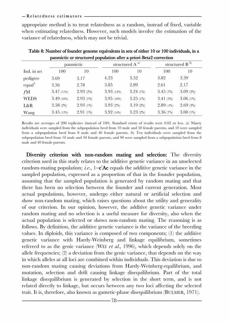
-------------------- R e l a t e d n e s s e s t i m a t o r s R e l a t e d n e s s e s t i m a t o r s R e l a t e d n e s s e s t i m a t o r s R e l a t e d n e s s e s t i m a t o r s --------------------------------------------------------------------------------------------------------------------------------------------------------------------------------------------------------------------------------------------------------------------------------------------------------------------------------------------------------------------------------------------------------------------------------------------------------------------------------------------------------------------------------------------------------------------------------------------------------------------------------------------------------------------------------------------------------------------------------------------------------------------------------------------------------------------------------------------------------
-------------------------------------------------------------------------------------------------------------------------------------------------------------------------------------------------------------------------------------------------------------------------------------------------------------------------------------------------------------------------------------------------------------------------------------------------------------------------------------------------------------------------------------------------------------------------------------------------------------------------------------------- ----------------------------------------------------------------------------------------------------------------------------------------------------------------------------------------------------------------------------------------------------------------------------------------------------------------------------------------------------------------------------------------------------------------------------------------------------------------------------------------------------------------------------------------------------------------------------------------------------------------
78
appropriate method is to treat relatedness as a random, instead of fixed, variable when estimating relatedness. However, such models involve the estimation of the variance of relatedness, which may not be trivial.
Table 8: Number of founder genome equivalents in sets of either 10 or 100 inTable 8: Number of founder genome equivalents in sets of either 10 or 100 inTable 8: Number of founder genome equivalents in sets of either 10 or 100 inTable 8: Number of founder genome equivalents in sets of either 10 or 100 individuals, in a dividuals, in a dividuals, in a dividuals, in a
panmictic or structured population after apanmictic or structured population after apanmictic or structured population after apanmictic or structured population after a----prioriprioriprioripriori----Beta2Beta2Beta2Beta2----correctioncorrectioncorrectioncorrection panmictic structured A (a) structured B (b)
Ind. in set 100 10 100 10 100 10
pedigree 3.69 3.17 4.23 3.52 3.82 3.39
equal3 3.56 2.78 3.85 2.89 2.61 2.17
ƒM 3.47 (11%) 2.93 (2%) 3.93 (12%) 3.24 (1%) 3.45 (7%) 3.09 (2%)
WEDS 3.49 (10%) 2.93 (1%) 3.95 (10%) 3.25 (1%) 3.41 (5%) 3.06 (1%)
L&R 3.58 (2%) 2.93 (1%) 3.93 (2%) 3.19 (2%) 2.89 (-2%) 2.69 (3%)
Wang 3.45 (12%) 2.91 (1%) 3.92 (14%) 3.23 (2%) 3.36 (7%) 3.00 (1%)
Results are averages of 200 replicates (instead of 100). Standard errors of results were 0.02 or less. (a) Ninety individuals were sampled from the subpopulation bred from 10 male and 50 female parents, and 10 were sampled from a subpopulation bred from 8 male and 40 female parents. (b) Ten individuals were sampled from the subpopulation bred from 10 male and 50 female parents, and 90 were sampled from a subpopulation bred from 8 male and 40 female parents.
Diversity criterion wDiversity criterion wDiversity criterion wDiversity criterion with nonith nonith nonith non----random mating and selection:random mating and selection:random mating and selection:random mating and selection: The diversity
criterion used in this study relates to the additive genetic variance in an unselected random-mating population; i.e., 1−cccc’AcAcAcAc equals the additive genetic variance in the sampled population, expressed as a proportion of that in the founder population, assuming that the sampled population is generated by random mating and that there has been no selection between the founder and current generation. Most actual populations, however, undergo either natural or artificial selection and show non-random mating, which raises questions about the utility and generality of our criterion. In our opinion, however, the additive genetic variance under random mating and no selection is a useful measure for diversity, also when the actual population is selected or shows non-random mating. The reasoning is as follows. By definition, the additive genetic variance is the variance of the breeding values. In diploids, this variance is composed of two components; (1) the additive genetic variance with Hardy-Weinberg and linkage equilibrium, sometimes referred to as the genic variance (WEI et al., 1996), which depends solely on the allele frequencies; (2) a deviation from the genic variance, that depends on the way in which alleles at all loci are combined within individuals. This deviation is due to non-random mating causing deviations from Hardy-Weinberg-equilibrium, and mutation, selection and drift causing linkage disequilibrium. Part of the total linkage disequilibrium is generated by selection in the short term, and is not related directly to linkage, but occurs between any two loci affecting the selected trait. It is, therefore, also known as gametic-phase disequilibrium (BULMER, 1971).
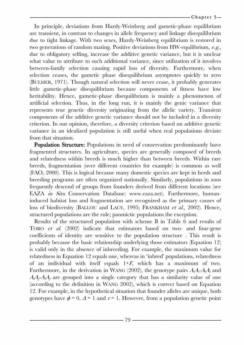
------------------------------------------------------------------------------------------------------------------------------------------------------------------------------------------------------------------------------------------------------------------------------------------------------------------------------------------------------------------------------------------------------------------------------------------------------------------------------------------------------------------------------------------------------------------------------------------------------------------------------------------------------------------------------------------------------------------------------------------------------------------------------------------------------------------------------------------------------------------------------------------------------------------------------------------------------------------------------------------------------------------------------------------------------------------------------------------------ C h a p t e r C h a p t e r C h a p t e r C h a p t e r 5555 --------------------
---------------------------------------------------------------------------------------------------------------------------------------------------------------------------------------------------------------------------------------------------------------------------------------------------------------------------------------------------------------------------------------------------------------------------------------------------------------------------------------------------------------------------------------------------------------------------------------------------------------------------------------- --------------------------------------------------------------------------------------------------------------------------------------------------------------------------------------------------------------------------------------------------------------------------------------------------------------------------------------------------------------------------------------------------------------------------------------------------------------------------------------------------------------------------------------------------------------------------------------------------------
79
In principle, deviations from Hardy-Weinberg and gametic-phase equilibrium are transient, in contrast to changes in allele frequency and linkage disequilibrium due to tight linkage. With two sexes, Hardy-Weinberg equilibrium is restored in two generations of random mating. Positive deviations from HW-equilibrium, e.g., due to obligatory selfing, increase the additive genetic variance, but it is unclear what value to attribute to such additional variance, since utilization of it involves between-family selection causing rapid loss of diversity. Furthermore, when selection ceases, the gametic phase disequilibrium asymptotes quickly to zero (BULMER, 1971). Though natural selection will never cease, it probably generates little gametic-phase disequilibrium because components of fitness have low heritability. Hence, gametic-phase disequilibrium is mainly a phenomenon of artificial selection. Thus, in the long run, it is mainly the genic variance that represents true genetic diversity originating from the allelic variety. Transient components of the additive genetic variance should not be included in a diversity criterion. In our opinion, therefore, a diversity criterion based on additive genetic variance in an idealized population is still useful when real populations deviate from that situation.
Population Structure:Population Structure:Population Structure:Population Structure: Populations in need of conservation predominantly have fragmented structures. In agriculture, species are generally composed of breeds and relatedness within breeds is much higher than between breeds. Within rare breeds, fragmentation (over different countries for example) is common as well (FAO, 2000). This is logical because many domestic species are kept in herds and breeding programs are often organized nationally. Similarly, populations in zoos frequently descend of groups from founders derived from different locations (see EAZA in Situ Conservation Database: www.eaza.net). Furthermore, human-induced habitat loss and fragmentation are recognized as the primary causes of loss of biodiversity (BALLOU and LACY, 1995; FRANKHAM et al., 2002). Hence, structured populations are the rule; panmictic populations the exception.
Results of the structured population with scheme B in Table 6 and results of TORO et al. (2002) indicate that estimators based on two- and four-gene coefficients of identity are sensitive to the population structure . This result is probably because the basic relationship underlying those estimators (Equation 12) is valid only in the absence of inbreeding. For example, the maximum value for relatedness in Equation 12 equals one, whereas in ‘inbred’ populations, relatedness of an individual with itself equals 1+F, which has a maximum of two. Furthermore, in the derivation in WANG (2002), the genotype pairs AiAi-AiAi and AiAj-AiAj are grouped into a single category that has a similarity value of one (according to the definition in WANG 2002), which is correct based on Equation 12. For example, in the hypothetical situation that founder alleles are unique, both genotypes have φ = 0, ∆ = 1 and r = 1. However, from a population genetic point
-------------------- R e l a t e d n e s s e s t i m a t o r s R e l a t e d n e s s e s t i m a t o r s R e l a t e d n e s s e s t i m a t o r s R e l a t e d n e s s e s t i m a t o r s --------------------------------------------------------------------------------------------------------------------------------------------------------------------------------------------------------------------------------------------------------------------------------------------------------------------------------------------------------------------------------------------------------------------------------------------------------------------------------------------------------------------------------------------------------------------------------------------------------------------------------------------------------------------------------------------------------------------------------------------------------------------------------------------------------------------------------------------------------
-------------------------------------------------------------------------------------------------------------------------------------------------------------------------------------------------------------------------------------------------------------------------------------------------------------------------------------------------------------------------------------------------------------------------------------------------------------------------------------------------------------------------------------------------------------------------------------------------------------------------------------------- ----------------------------------------------------------------------------------------------------------------------------------------------------------------------------------------------------------------------------------------------------------------------------------------------------------------------------------------------------------------------------------------------------------------------------------------------------------------------------------------------------------------------------------------------------------------------------------------------------------------
80
of view, those genotype pairs are clearly different; AiAi-AiAi has ƒ= 1 and r = 2, whereas AiAj-AiAj has ƒ= ½ and r = 1.
When noting that the basic equation underlying the L&R and the Wang-estimator is invalid with inbreeding, the good performance of those estimators in ‘inbred’ panmictic populations seem surprising as first. However, as argued above, the definition of a base population is arbitrary with a panmictic population. Occurrence of inbreeding, therefore, does not present a problem with random mating, because inbreeding coefficients can be shifted to approximately zero by redefining the base population. The L&R and Wang-estimators “remove” inbreeding by determining the probability that alleles are AIS based on observed allele frequencies, which defines the base population to be equal to the current population. The same would happen if sl in Equation (3) would be set on the currently expected homozygosity, as in RITLAND (1996). In a structured population, however, removing inbreeding by using the current population as base population causes negative (true) coancestries between individuals in different subpopulations, which is theoretically incorrect. In structured populations, therefore, inbreeding cannot be removed by shifting the base population. We believe that the inability to fully remove inbreeding is the basis of the poor performance of the L&R-estimator in scheme B of the structured population. The high number of founder genome equivalents of L&R with scheme A in Table 7, is probably because scheme A resembles a panmictic population, since the low number of sampled individuals from the high drift population are in balance with low contribution in diversity of this sample. The β2 correction hardly improves founder genome equivalents for L&R, whereas it improves all other estimators (Table 8).
Our results show that benefits of using relatedness estimates in conservation programs is substantially larger in structured than in panmictic populations (Table 7; FERNANDEZ et al. 2005). What is needed in practice, therefore, is an estimator that can be applied to general populations. The WEDS-estimator is based on: (1) the relationship between relatedness and coancestry (r = 2ƒ), and (2) the relationship between molecular similarity and coancestry (Equation 2a). Both relationships are valid irrespective of the population structure (LYNCH, 1988; FALCONER and MACKAY, 1996), and provide the theoretical basis for an estimator of both within and between population relatedness (EDING and MEUWISSEN, 2001).
We obtained the WEDS-estimator using a simple statistical approach, in which expected similarity was equated to observed similarity (Equation 3). Good results of the L&R-estimator in panmictic populations indicate that estimators can be improved by using a more advanced statistical approach, such as conditional probabilities of observing genotypes, rather than similarity values. Hence, a promising approach to develop an estimator that performs better in both
------------------------------------------------------------------------------------------------------------------------------------------------------------------------------------------------------------------------------------------------------------------------------------------------------------------------------------------------------------------------------------------------------------------------------------------------------------------------------------------------------------------------------------------------------------------------------------------------------------------------------------------------------------------------------------------------------------------------------------------------------------------------------------------------------------------------------------------------------------------------------------------------------------------------------------------------------------------------------------------------------------------------------------------------------------------------------------------------ C h a p t e r C h a p t e r C h a p t e r C h a p t e r 5555 --------------------
---------------------------------------------------------------------------------------------------------------------------------------------------------------------------------------------------------------------------------------------------------------------------------------------------------------------------------------------------------------------------------------------------------------------------------------------------------------------------------------------------------------------------------------------------------------------------------------------------------------------------------------- --------------------------------------------------------------------------------------------------------------------------------------------------------------------------------------------------------------------------------------------------------------------------------------------------------------------------------------------------------------------------------------------------------------------------------------------------------------------------------------------------------------------------------------------------------------------------------------------------------
81
panmictic and structured populations is to follow the statistical approach of LYNCH and RITLAND (1999), but using r = 2ƒ and the similarity definition of Equation 1 as starting point (see also TORO et al. 2002).
Use in conservation practice:Use in conservation practice:Use in conservation practice:Use in conservation practice: Benefit of optimal contributions based on relatedness estimators in conservation programs depends on the population structure and on the breeding capacity available for conservation, e.g. expressed as the size of a population that can be conserved (N). The use of optimal contributions based on relatedness estimates that are regressed to their mean, always maintains more diversity than applying equal contributions (Table 8), when populations are structured, which is common for populations in need of conservation. Even when they are panmictic and there is a limited breeding capacity (e.g. N = 10), optimal contributions based on relatedness estimates are beneficial. With panmictic populations and large capacity, it is equally good or better to use equal instead of optimal contributions (Table 8, N = 100), though this is seldom the case in conservation.
When using Equation 22 to regress estimates to their mean value, ƒM and WEDS are overall the best estimators. They are robust with respect to population structure, which is important when it is unknown whether the population is truly panmictic.
More information and partial Fortran code can be found on: http://www.geneticdiversity.net/estimators.html
AAAACKNOWLEDGEMENTCKNOWLEDGEMENTCKNOWLEDGEMENTCKNOWLEDGEMENT We thank Sipke Joost Hiemstra of CGN for his thorough comments on previous
versions. Thanks are also due to Jinliang Wang for making the Fortran-code of his estimator available on internet. This work was financed by the Ministry of Agriculture, Nature and Food Quality through the Centre for Genetic Resources, the Netherlands (CGN).
. . .

----------------------------------------------------------------------------------------------------------------------------------------------------------------------------------------------------------------------------------------------------------------------------------------------------------------------------------------------------------------------------------------------------------------------------------------------------------------------------------------------------------------------------------------------------------------------------------------------------------------------------------------------------------------------------------------------------------------------------------------------------------------------------------------------------------------------------------------------------------------------------------------------------------------------------------------------------------------------------------------------------------------------------------------------------------------------------------------------------------------------------------------------------------------------------------------------------------------------------------------------------------------------------------------------------------------
-------------------------------------------------------------------------------------------------------------------------------------------------------------------------------------------------------------------------------------------------------------------------------------------------------------------------------------------------------------------------------------------------------------------------------------------------------------------------------------------------------------------------------------------------------------------------------------------------------------------------------------------- ----------------------------------------------------------------------------------------------------------------------------------------------------------------------------------------------------------------------------------------------------------------------------------------------------------------------------------------------------------------------------------------------------------------------------------------------------------------------------------------------------------------------------------------------------------------------------------------------------------------
82
----------------------------------------------------------------------------------------------------------------------------------------------------------------------------------------------------------------------------------------------------------------------------------------------------------------------------------------------------------------------------------------------------------------------------------------------------------------------------------------------------------------------------------------------------------------------------------------------------------------------------------------------------------------------------------------------------------------------------------------------------------------------------------------------------------------------------------------------------------------------------------------------------------------------------------------------------------------------------------------------------------------------------------------------------------------------------------------------------------------------------------------------------------------------------------------------------------------------------------------------------------------------------------------------------------------
-------------------------------------------------------------------------------------------------------------------------------------------------------------------------------------------------------------------------------------------------------------------------------------------------------------------------------------------------------------------------------------------------------------------------------------------------------------------------------------------------------------------------------------------------------------------------------------------------------------------------------------------- ----------------------------------------------------------------------------------------------------------------------------------------------------------------------------------------------------------------------------------------------------------------------------------------------------------------------------------------------------------------------------------------------------------------------------------------------------------------------------------------------------------------------------------------------------------------------------------------------------------------
83
General DiscussionGeneral DiscussionGeneral DiscussionGeneral Discussion
C h a p t e r 6C h a p t e r 6C h a p t e r 6C h a p t e r 6 This thesis has investigated the possibilities to increase or maintain genetic
diversity within small animal populations. The focus has been on genetic diversity saved by conservation measures when the observed kinship, obtained from pedigree or molecular markers, deviates from true kinship. This thesis describes the relative loss of genetic diversity due to these deviations from true kinship (when true genealogy was known; Chapter 2, 3, 5) and possibilities for correction of detected or predicted deviations (Chapter 4, 5).
Both panmictic and structured populations were analyzed. Panmictic populations often serve as a model in theoretical and simulation studies. This Chapter, however, will mainly discuss small populations in captivity that are in need of conservation considering livestock breeds as well as wild (sub-)species, for example present in zoos. Populations like these often have three characteristics that increase genetic drift: fluctuating populations sizes; few founders that initiated the captive breeding population (RUDNICK and LACY, 2008); unequal contributions of parents to subsequent generations (FRANKHAM et al., 2002). Furthermore, these populations have a recent history in studbook formation and are often fragmented. Implications of previous chapters will be discussed for this type of populations, which will hereafter be referred to as ‘small captive populations’. This chapter discusses: the meaning of founders for this type of populations; some practical examples of the populations in study; the influence of pedigree errors is discussed; conservation by means of selection; and finally biodiversity loss and its relation to collapses of civilizations.
BBBBASE POPULATIONASE POPULATIONASE POPULATIONASE POPULATION,,,, FFFFOUNDERS AND OUNDERS AND OUNDERS AND OUNDERS AND FFFFOUNDER OUNDER OUNDER OUNDER GGGGENOME ENOME ENOME ENOME EEEEQUIVALENTSQUIVALENTSQUIVALENTSQUIVALENTS When pedigrees are considered, the base population consists of founders (see
GENERAL INTRODUCTION). The definition of the base population when kinship is calculated from molecular markers is discussed in Chapter 1 and 5. In both cases the definition of a base population is arbitrary since evolution of populations is an ongoing process. With a constant size, large populations establish a balance between selection, mutation and drift. In larger populations, especially when breeding is random (panmixia or in other words the population is not structured), the base population primarily facilitates our understanding of populations, enable estimation of kinship and estimation of heritability. In contrast, small captive populations often have few founders in comparison with the current population
-------------------- G e n e r a l D i s c u s s i o n G e n e r a l D i s c u s s i o n G e n e r a l D i s c u s s i o n G e n e r a l D i s c u s s i o n ------------------------------------------------------------------------------------------------------------------------------------------------------------------------------------------------------------------------------------------------------------------------------------------------------------------------------------------------------------------------------------------------------------------------------------------------------------------------------------------------------------------------------------------------------------------------------------------------------------------------------------------------------------------------------------------------------------------------------------------------------------------------------------------------------------------------------------------------------------------------------------------------------------------------
-------------------------------------------------------------------------------------------------------------------------------------------------------------------------------------------------------------------------------------------------------------------------------------------------------------------------------------------------------------------------------------------------------------------------------------------------------------------------------------------------------------------------------------------------------------------------------------------------------------------------------------------- ----------------------------------------------------------------------------------------------------------------------------------------------------------------------------------------------------------------------------------------------------------------------------------------------------------------------------------------------------------------------------------------------------------------------------------------------------------------------------------------------------------------------------------------------------------------------------------------------------------------
84
size. Furthermore, small captive populations often have a high variance of reproductive success among parents, compared to panmictic populations, which most likely increases loss of diversity. Due to this loss and the small population size, the effect of mutations are negligible, and thus small captive populations will usually not obtain higher levels of genetic diversity than was present in founders. In addition, the selection pressure for small captive populations of wild species will strongly differ from their wild habitat. Hence, a balance between selection, mutation and drift is not expected. Thus in contrast to panmictic populations, founders are biological relevant in small captive populations. Therefore, the founders are an obvious choice as base population and genetic diversity relative to those founders is meaningful.
Founders are assumed unrelated by definition. In practice, founders are animals from the wild or thought to have no close relation with the other founders. This assumption might hold not in practice. For example, when an entire litter is introduced from the wild, their father and mother should be registered as founders and not the newborns. Also in other cases is likely that some founders are more related to each other than to other founders. Therefore, the influence of kinship among founders on conservation strategies is relevant. RUDNICK and LACY (2008) investigated the influence of unknown kinship among founders on expected heterozygosity maintained. When true kinship was known the expected heterozygosity maintained by breeding was at most a 2% higher than for cases that true kinship of founders was not known. To maintain genetic diversity, RUDNICK and LACY (2008) applied a conservation strategy based on mean kinship. Optimal contribution selection is more ‘sensitive’ to variation in kinships among individuals. On the other hand, founders are often found many generations back, so that their contributions are often already fixed in the current population. Overall, founders are a reliable starting point for judging genetic variation in small captive populations, though possible relatedness among founders should be taken into account when optimal contribution selection is applied in initial generations after first founders.
Hence it is meaningful to compare genetic variation of the small captive populations with its founders (the base population). In this research genetic diversity (Nmk), potential (genetic) diversity (NOC), and allelic diversity (NAD) are expressed on the scale of founder genome equivalents (see GENERAL
INTRODUCTION). Unlike measures as average mean kinship or the average or rate of inbreeding, founder genome equivalents gives direct insight in the actual loss of variation in relation to the original diversity of founders (CABALLERO and TORO, 2000). Furthermore, genetic diversity of the base population itself is equal to the number of founders in the base population. Hence, genetic diversity can never be higher than the number of founders. EDING et al. (2002) and EDING and MEUWISSEN (2003) used the scale of founder genome equivalents for a different
------------------------------------------------------------------------------------------------------------------------------------------------------------------------------------------------------------------------------------------------------------------------------------------------------------------------------------------------------------------------------------------------------------------------------------------------------------------------------------------------------------------------------------------------------------------------------------------------------------------------------------------------------------------------------------------------------------------------------------------------------------------------------------------------------------------------------------------------------------------------------------------------------------------------------------------------------------------------------------------------------------------------------------------------------------------------------------------------ C h a p t e r C h a p t e r C h a p t e r C h a p t e r 6666 --------------------
---------------------------------------------------------------------------------------------------------------------------------------------------------------------------------------------------------------------------------------------------------------------------------------------------------------------------------------------------------------------------------------------------------------------------------------------------------------------------------------------------------------------------------------------------------------------------------------------------------------------------------------- --------------------------------------------------------------------------------------------------------------------------------------------------------------------------------------------------------------------------------------------------------------------------------------------------------------------------------------------------------------------------------------------------------------------------------------------------------------------------------------------------------------------------------------------------------------------------------------------------------
85
reason. They investigated the contribution of individual breeds to the overall genetic variation of selected set of breeds for conservation in chicken and cows. They found that absolute values of genetic variation contributed by individual breeds were rather small, while the losses expressed in founder genome equivalents were substantially larger, when certain breeds were removed from the complete set. They also found that ranking of breeds was not affected by a change of scale, which is easy to explain mathematically (see GENERAL INTRODUCTION: Table 1). The same result was found when kinship estimators were evaluated (Chapter 5) and influence of pedigree errors was investigated (Chapter 3 and 4). Another reason for the scale of founder genome equivalents is that allelic diversity is linked to the number of alleles still surviving in the present population, which itself is related to limits of selection on the long term. Finally, a scale like founder genome equivalents is better comprehensible because they are natural numbers rather than proportions or frequencies (HOFFRAGE et al., 2000). Note that effective population size (Ne; GENERAL INTRODUCTION: Table 1), is expressed on a similar scale, but relative to the previous generation. An effective population size can therefore be infinitive or even negative, while genetic diversity (and potential and allelic diversity) always ranges between 0.5 (a completely inbred strain) and the population size (when all individuals are founders).
CCCCONSERVATIONONSERVATIONONSERVATIONONSERVATION,,,, PEDIGREE ERRORS AND PEDIGREE ERRORS AND PEDIGREE ERRORS AND PEDIGREE ERRORS AND POPULATON STRUCTUREPOPULATON STRUCTUREPOPULATON STRUCTUREPOPULATON STRUCTURE Most small captive populations have pedigree records. When pedigrees are
reliable, this information is an obvious choice for conservation schemes. However, pedigrees often contain errors. Species coordinators warned that recorded pedigrees do not always represent the true situation (Chapter 4). Also within domestic species, the recorded pedigree can contain errors (Chapter 3: Table 1). This thesis investigated influence of pedigree errors on conservation of genetic diversity (Chapter 3) and investigated options to correct for unknown parents (Chapter 4).
There are two types of pedigrees errors: (1) unknown (missing) parentage; (2) undetected wrong parentage. Chapter 3 is consistent with Chapter 4 about how to deal with unknown parents: kinship based on pedigree with unknown parent information should always be corrected. Otherwise, conservation methods will select predominantly animals that descend from unknown parents, since they appear unrelated while they are not. However, Chapter 3 seems inconsistent with Chapter 4 on when and how to act upon undetected wrong parentage. Chapter 3 concludes from simulated panmictic populations, that a strategy similar to equal contributions is likely to preserve more genetic diversity than optimal contribution selection, in the case that the percentage of wrong parentage exceeds 35%. With increasing percentage of wrong parents, the increase of genetic diversity due to optimal contribution selection is strongly hampered. BAUMUNG
-------------------- G e n e r a l D i s c u s s i o n G e n e r a l D i s c u s s i o n G e n e r a l D i s c u s s i o n G e n e r a l D i s c u s s i o n ------------------------------------------------------------------------------------------------------------------------------------------------------------------------------------------------------------------------------------------------------------------------------------------------------------------------------------------------------------------------------------------------------------------------------------------------------------------------------------------------------------------------------------------------------------------------------------------------------------------------------------------------------------------------------------------------------------------------------------------------------------------------------------------------------------------------------------------------------------------------------------------------------------------------
-------------------------------------------------------------------------------------------------------------------------------------------------------------------------------------------------------------------------------------------------------------------------------------------------------------------------------------------------------------------------------------------------------------------------------------------------------------------------------------------------------------------------------------------------------------------------------------------------------------------------------------------- ----------------------------------------------------------------------------------------------------------------------------------------------------------------------------------------------------------------------------------------------------------------------------------------------------------------------------------------------------------------------------------------------------------------------------------------------------------------------------------------------------------------------------------------------------------------------------------------------------------------
86
and SÖLKNER (2003) suggested that under non-panmictic schemes, the demand on quality of pedigree records even increases. However, Chapter 4 concludes that optimal contribution selection would increase genetic diversity, despite pedigree errors even with uncorrected unknown parents. This conclusion is illustrated by the diversity saved by C1-correction, a correction method that assigns parents randomly for animals that have unknown parents. These random assigned parents were often the ‘wrong’ parents. Hence, the C1-correction acts like a simulated wrong parentage test. For example, the diversity saved with these ‘simulated pedigree errors’ in African wild dog was still 0.9 on average. In Chapter 3 the diversity saved was only 0.62 (Figure 2). There are two factors causing these differences between Chapter 3 and 4. (1) The three zoo-populations had relative less unknown parents during the last generations, while error probabilities in Chapter 3 were equal in every generation. This factor is probably less influential. (2) Chapter 4 also shows that potential diversity is almost twice the genetic diversity for the three zoo populations under study. The difference between genetic diversity and potential diversity in Chapter 3 was very low, due to panmixia. Thus, in small captive populations the gain due to the difference between actual and potential genetic diversity outpaces the loss due to undetected wrong parentage. A similar conclusion was drawn in Chapter 5, which investigated possibilities to increase genetic diversity with the aid of molecular markers in both panmictic and structured populations. In conclusion, despite wrong parentage decreases feasibility to maximize genetic diversity, it is still beneficial to apply optimal contribution selection in small captive populations, because they are structured.
DDDDIVERSITY IVERSITY IVERSITY IVERSITY MMMMEASURES AND EASURES AND EASURES AND EASURES AND PPPPOPULATION OPULATION OPULATION OPULATION SSSSTRUCTURETRUCTURETRUCTURETRUCTURE The rate of inbreeding is regarded as a good diversity measure and is often used
within population genetics (FALCONER and MACKAY, 1996; LYNCH and WALSH, 1997). The paragraph above shows that the population structure affects diversity measures. The rate of inbreeding might behave different in panmictic and structured populations. For this reason, small captive populations were analyzed throughout their population history for demographic parameters and diversity measures as described in Chapter 1.
Figures 1, 2 and 3 show the European zoo population history of the giraffe (Giraffa camelopardalis) and the African wild dog (Lycaon pictus); black-footed cat (Felis nigripes), as described in Chapter 4. Figures 4 and 5 show the global population history of the red panda (Ailurus fulgens) and the cheetah (Acinonyx jubatus). Data of cheetah was obtained from the International Studbook Keeper (MARKER, 2008). A maximal life expectancy was estimated for males and females separately from the interval between date of birth of parents and progeny. If date of death was not recorded, it was estimated by this life expectancy. All animals
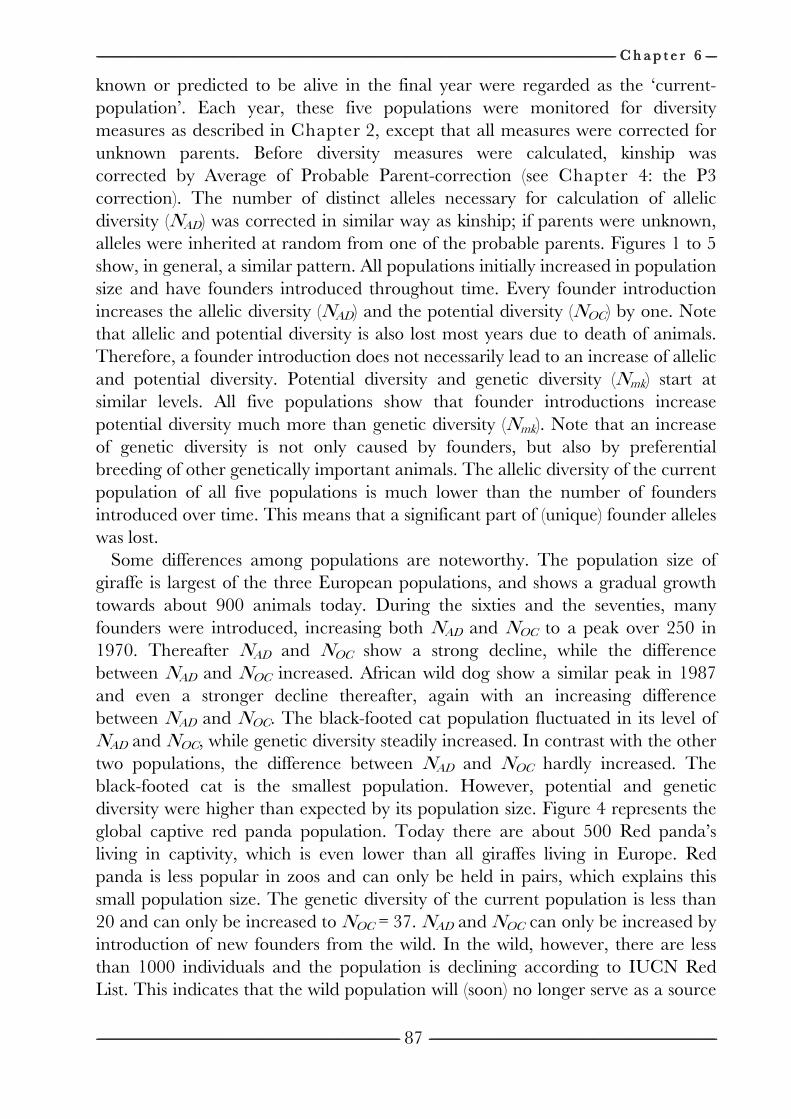
------------------------------------------------------------------------------------------------------------------------------------------------------------------------------------------------------------------------------------------------------------------------------------------------------------------------------------------------------------------------------------------------------------------------------------------------------------------------------------------------------------------------------------------------------------------------------------------------------------------------------------------------------------------------------------------------------------------------------------------------------------------------------------------------------------------------------------------------------------------------------------------------------------------------------------------------------------------------------------------------------------------------------------------------------------------------------------------------ C h a p t e r C h a p t e r C h a p t e r C h a p t e r 6666 --------------------
---------------------------------------------------------------------------------------------------------------------------------------------------------------------------------------------------------------------------------------------------------------------------------------------------------------------------------------------------------------------------------------------------------------------------------------------------------------------------------------------------------------------------------------------------------------------------------------------------------------------------------------- --------------------------------------------------------------------------------------------------------------------------------------------------------------------------------------------------------------------------------------------------------------------------------------------------------------------------------------------------------------------------------------------------------------------------------------------------------------------------------------------------------------------------------------------------------------------------------------------------------
87
known or predicted to be alive in the final year were regarded as the ‘current-population’. Each year, these five populations were monitored for diversity measures as described in Chapter 2, except that all measures were corrected for unknown parents. Before diversity measures were calculated, kinship was corrected by Average of Probable Parent-correction (see Chapter 4: the P3 correction). The number of distinct alleles necessary for calculation of allelic diversity (NAD) was corrected in similar way as kinship; if parents were unknown, alleles were inherited at random from one of the probable parents. Figures 1 to 5 show, in general, a similar pattern. All populations initially increased in population size and have founders introduced throughout time. Every founder introduction increases the allelic diversity (NAD) and the potential diversity (NOC) by one. Note that allelic and potential diversity is also lost most years due to death of animals. Therefore, a founder introduction does not necessarily lead to an increase of allelic and potential diversity. Potential diversity and genetic diversity (Nmk) start at similar levels. All five populations show that founder introductions increase potential diversity much more than genetic diversity (Nmk). Note that an increase of genetic diversity is not only caused by founders, but also by preferential breeding of other genetically important animals. The allelic diversity of the current population of all five populations is much lower than the number of founders introduced over time. This means that a significant part of (unique) founder alleles was lost.
Some differences among populations are noteworthy. The population size of giraffe is largest of the three European populations, and shows a gradual growth towards about 900 animals today. During the sixties and the seventies, many founders were introduced, increasing both NAD and NOC to a peak over 250 in 1970. Thereafter NAD and NOC show a strong decline, while the difference between NAD and NOC increased. African wild dog show a similar peak in 1987 and even a stronger decline thereafter, again with an increasing difference between NAD and NOC. The black-footed cat population fluctuated in its level of NAD and NOC, while genetic diversity steadily increased. In contrast with the other two populations, the difference between NAD and NOC hardly increased. The black-footed cat is the smallest population. However, potential and genetic diversity were higher than expected by its population size. Figure 4 represents the global captive red panda population. Today there are about 500 Red panda’s living in captivity, which is even lower than all giraffes living in Europe. Red panda is less popular in zoos and can only be held in pairs, which explains this small population size. The genetic diversity of the current population is less than 20 and can only be increased to NOC = 37. NAD and NOC can only be increased by introduction of new founders from the wild. In the wild, however, there are less than 1000 individuals and the population is declining according to IUCN Red List. This indicates that the wild population will (soon) no longer serve as a source
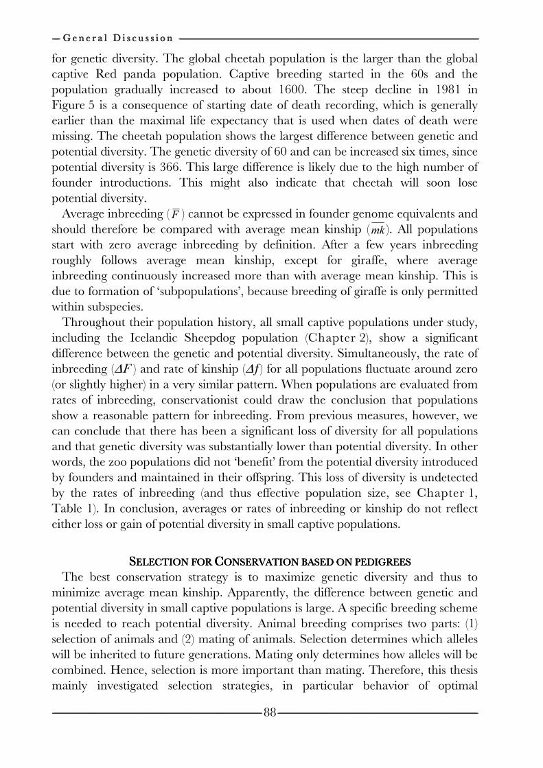
-------------------- G e n e r a l D i s c u s s i o n G e n e r a l D i s c u s s i o n G e n e r a l D i s c u s s i o n G e n e r a l D i s c u s s i o n ------------------------------------------------------------------------------------------------------------------------------------------------------------------------------------------------------------------------------------------------------------------------------------------------------------------------------------------------------------------------------------------------------------------------------------------------------------------------------------------------------------------------------------------------------------------------------------------------------------------------------------------------------------------------------------------------------------------------------------------------------------------------------------------------------------------------------------------------------------------------------------------------------------------------
-------------------------------------------------------------------------------------------------------------------------------------------------------------------------------------------------------------------------------------------------------------------------------------------------------------------------------------------------------------------------------------------------------------------------------------------------------------------------------------------------------------------------------------------------------------------------------------------------------------------------------------------- ----------------------------------------------------------------------------------------------------------------------------------------------------------------------------------------------------------------------------------------------------------------------------------------------------------------------------------------------------------------------------------------------------------------------------------------------------------------------------------------------------------------------------------------------------------------------------------------------------------------
88
for genetic diversity. The global cheetah population is the larger than the global captive Red panda population. Captive breeding started in the 60s and the population gradually increased to about 1600. The steep decline in 1981 in Figure 5 is a consequence of starting date of death recording, which is generally earlier than the maximal life expectancy that is used when dates of death were missing. The cheetah population shows the largest difference between genetic and potential diversity. The genetic diversity of 60 and can be increased six times, since potential diversity is 366. This large difference is likely due to the high number of founder introductions. This might also indicate that cheetah will soon lose potential diversity.
Average inbreeding (F ) cannot be expressed in founder genome equivalents and should therefore be compared with average mean kinship (mk ). All populations start with zero average inbreeding by definition. After a few years inbreeding roughly follows average mean kinship, except for giraffe, where average inbreeding continuously increased more than with average mean kinship. This is due to formation of ‘subpopulations’, because breeding of giraffe is only permitted within subspecies.
Throughout their population history, all small captive populations under study, including the Icelandic Sheepdog population (Chapter 2), show a significant difference between the genetic and potential diversity. Simultaneously, the rate of inbreeding (∆F ) and rate of kinship (∆ƒ) for all populations fluctuate around zero (or slightly higher) in a very similar pattern. When populations are evaluated from rates of inbreeding, conservationist could draw the conclusion that populations show a reasonable pattern for inbreeding. From previous measures, however, we can conclude that there has been a significant loss of diversity for all populations and that genetic diversity was substantially lower than potential diversity. In other words, the zoo populations did not ‘benefit’ from the potential diversity introduced by founders and maintained in their offspring. This loss of diversity is undetected by the rates of inbreeding (and thus effective population size, see Chapter 1, Table 1). In conclusion, averages or rates of inbreeding or kinship do not reflect either loss or gain of potential diversity in small captive populations.
SSSSELECTION FOR ELECTION FOR ELECTION FOR ELECTION FOR CCCCONSERVATION BASED ONONSERVATION BASED ONONSERVATION BASED ONONSERVATION BASED ON PEDIGREESPEDIGREESPEDIGREESPEDIGREES The best conservation strategy is to maximize genetic diversity and thus to
minimize average mean kinship. Apparently, the difference between genetic and potential diversity in small captive populations is large. A specific breeding scheme is needed to reach potential diversity. Animal breeding comprises two parts: (1) selection of animals and (2) mating of animals. Selection determines which alleles will be inherited to future generations. Mating only determines how alleles will be combined. Hence, selection is more important than mating. Therefore, this thesis mainly investigated selection strategies, in particular behavior of optimal
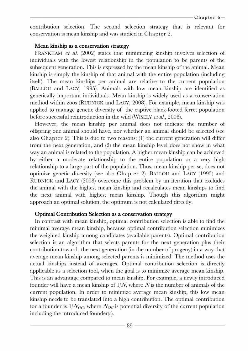
------------------------------------------------------------------------------------------------------------------------------------------------------------------------------------------------------------------------------------------------------------------------------------------------------------------------------------------------------------------------------------------------------------------------------------------------------------------------------------------------------------------------------------------------------------------------------------------------------------------------------------------------------------------------------------------------------------------------------------------------------------------------------------------------------------------------------------------------------------------------------------------------------------------------------------------------------------------------------------------------------------------------------------------------------------------------------------------------ C h a p t e r C h a p t e r C h a p t e r C h a p t e r 6666 --------------------
---------------------------------------------------------------------------------------------------------------------------------------------------------------------------------------------------------------------------------------------------------------------------------------------------------------------------------------------------------------------------------------------------------------------------------------------------------------------------------------------------------------------------------------------------------------------------------------------------------------------------------------- --------------------------------------------------------------------------------------------------------------------------------------------------------------------------------------------------------------------------------------------------------------------------------------------------------------------------------------------------------------------------------------------------------------------------------------------------------------------------------------------------------------------------------------------------------------------------------------------------------
89
contribution selection. The second selection strategy that is relevant for conservation is mean kinship and was studied in Chapter 2.
Mean kinship as a conservation strategyMean kinship as a conservation strategyMean kinship as a conservation strategyMean kinship as a conservation strategy FRANKHAM et al. (2002) states that minimizing kinship involves selection of
individuals with the lowest relationship in the population to be parents of the subsequent generation. This is expressed by the mean kinship of the animal. Mean kinship is simply the kinship of that animal with the entire population (including itself). The mean kinships per animal are relative to the current population (BALLOU and LACY, 1995). Animals with low mean kinship are identified as genetically important individuals. Mean kinship is widely used as a conservation method within zoos (RUDNICK and LACY, 2008). For example, mean kinship was applied to manage genetic diversity of the captive black-footed ferret population before successful reintroduction in the wild (WISELY et al., 2008).
However, the mean kinship per animal does not indicate the number of offspring one animal should have, nor whether an animal should be selected (see also Chapter 2). This is due to two reasons: (1) the current generation will differ from the next generation, and (2) the mean kinship level does not show in what way an animal is related to the population. A higher mean kinship can be achieved by either a moderate relationship to the entire population or a very high relationship to a large part of the population. Thus, mean kinship per se, does not optimize genetic diversity (see also Chapter 2). BALLOU and LACY (1995) and RUDNICK and LACY (2008) overcome this problem by an iteration that excludes the animal with the highest mean kinship and recalculates mean kinships to find the next animal with highest mean kinship. Though this algorithm might approach an optimal solution, the optimum is not calculated directly.
Optimal Contribution Selection as a conservation strategyOptimal Contribution Selection as a conservation strategyOptimal Contribution Selection as a conservation strategyOptimal Contribution Selection as a conservation strategy In contrast with mean kinship, optimal contribution selection is able to find the
minimal average mean kinship, because optimal contribution selection minimizes the weighted kinship among candidates (available parents). Optimal contribution selection is an algorithm that selects parents for the next generation plus their contribution towards the next generation (in the number of progeny) in a way that average mean kinship among selected parents is minimized. The method uses the actual kinships instead of averages. Optimal contribution selection is directly applicable as a selection tool, when the goal is to minimize average mean kinship. This is an advantage compared to mean kinship. For example, a newly introduced founder will have a mean kinship of 1/N, where N is the number of animals of the current population. In order to minimize average mean kinship, this low mean kinship needs to be translated into a high contribution. The optimal contribution for a founder is 1/NOC, where NOC is potential diversity of the current population including the introduced founder(s).
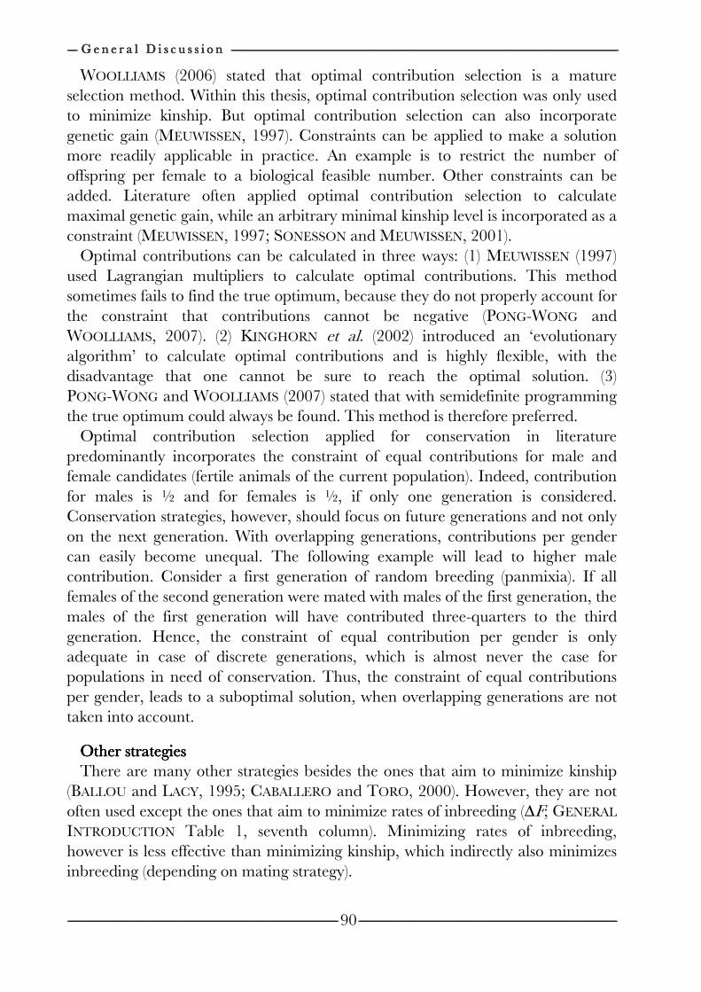
-------------------- G e n e r a l D i s c u s s i o n G e n e r a l D i s c u s s i o n G e n e r a l D i s c u s s i o n G e n e r a l D i s c u s s i o n ------------------------------------------------------------------------------------------------------------------------------------------------------------------------------------------------------------------------------------------------------------------------------------------------------------------------------------------------------------------------------------------------------------------------------------------------------------------------------------------------------------------------------------------------------------------------------------------------------------------------------------------------------------------------------------------------------------------------------------------------------------------------------------------------------------------------------------------------------------------------------------------------------------------------
-------------------------------------------------------------------------------------------------------------------------------------------------------------------------------------------------------------------------------------------------------------------------------------------------------------------------------------------------------------------------------------------------------------------------------------------------------------------------------------------------------------------------------------------------------------------------------------------------------------------------------------------- ----------------------------------------------------------------------------------------------------------------------------------------------------------------------------------------------------------------------------------------------------------------------------------------------------------------------------------------------------------------------------------------------------------------------------------------------------------------------------------------------------------------------------------------------------------------------------------------------------------------
90
WOOLLIAMS (2006) stated that optimal contribution selection is a mature selection method. Within this thesis, optimal contribution selection was only used to minimize kinship. But optimal contribution selection can also incorporate genetic gain (MEUWISSEN, 1997). Constraints can be applied to make a solution more readily applicable in practice. An example is to restrict the number of offspring per female to a biological feasible number. Other constraints can be added. Literature often applied optimal contribution selection to calculate maximal genetic gain, while an arbitrary minimal kinship level is incorporated as a constraint (MEUWISSEN, 1997; SONESSON and MEUWISSEN, 2001).
Optimal contributions can be calculated in three ways: (1) MEUWISSEN (1997) used Lagrangian multipliers to calculate optimal contributions. This method sometimes fails to find the true optimum, because they do not properly account for the constraint that contributions cannot be negative (PONG-WONG and WOOLLIAMS, 2007). (2) KINGHORN et al. (2002) introduced an ‘evolutionary algorithm’ to calculate optimal contributions and is highly flexible, with the disadvantage that one cannot be sure to reach the optimal solution. (3) PONG-WONG and WOOLLIAMS (2007) stated that with semidefinite programming the true optimum could always be found. This method is therefore preferred.
Optimal contribution selection applied for conservation in literature predominantly incorporates the constraint of equal contributions for male and female candidates (fertile animals of the current population). Indeed, contribution for males is ½ and for females is ½, if only one generation is considered. Conservation strategies, however, should focus on future generations and not only on the next generation. With overlapping generations, contributions per gender can easily become unequal. The following example will lead to higher male contribution. Consider a first generation of random breeding (panmixia). If all females of the second generation were mated with males of the first generation, the males of the first generation will have contributed three-quarters to the third generation. Hence, the constraint of equal contribution per gender is only adequate in case of discrete generations, which is almost never the case for populations in need of conservation. Thus, the constraint of equal contributions per gender, leads to a suboptimal solution, when overlapping generations are not taken into account.
Other strategiesOther strategiesOther strategiesOther strategies There are many other strategies besides the ones that aim to minimize kinship
(BALLOU and LACY, 1995; CABALLERO and TORO, 2000). However, they are not often used except the ones that aim to minimize rates of inbreeding (∆F; GENERAL
INTRODUCTION Table 1, seventh column). Minimizing rates of inbreeding, however is less effective than minimizing kinship, which indirectly also minimizes inbreeding (depending on mating strategy).
------------------------------------------------------------------------------------------------------------------------------------------------------------------------------------------------------------------------------------------------------------------------------------------------------------------------------------------------------------------------------------------------------------------------------------------------------------------------------------------------------------------------------------------------------------------------------------------------------------------------------------------------------------------------------------------------------------------------------------------------------------------------------------------------------------------------------------------------------------------------------------------------------------------------------------------------------------------------------------------------------------------------------------------------------------------------------------------------ C h a p t e r C h a p t e r C h a p t e r C h a p t e r 6666 --------------------
---------------------------------------------------------------------------------------------------------------------------------------------------------------------------------------------------------------------------------------------------------------------------------------------------------------------------------------------------------------------------------------------------------------------------------------------------------------------------------------------------------------------------------------------------------------------------------------------------------------------------------------- --------------------------------------------------------------------------------------------------------------------------------------------------------------------------------------------------------------------------------------------------------------------------------------------------------------------------------------------------------------------------------------------------------------------------------------------------------------------------------------------------------------------------------------------------------------------------------------------------------
91
Selection in practiceSelection in practiceSelection in practiceSelection in practice Conservation in practice is faced with constraints. Older animals will not be able
to produce progeny as long as younger animals. BALLOU and LACY (1995) proposed kinship value which is mean kinship weighted by the expected future reproduction per candidate. Animals that will soon be incapable of reproduction will have lower impact on kinship values. This might solve the problem that the mean kinship level does not show in what way an animal is related to the population. SONESSON and MEUWISSEN (2001) incorporated age classes as a constraint in optimal contribution calculations. They found that the algorithm favors older animals over younger ones. NOMURA (2005) stated that despite incorporation of constraints, the method of SONESSON and MEUWISSEN (2001) is difficult to apply in practice. NOMURA (2005) proposed a selection method that is similar to kinship values as described by BALLOU and LACY (1995). NOMURA (2005) stated that this method is less optimal, however better applicable.
The selection scheme and especially the number of progeny as calculated by the conservation strategy can indeed seldom be applied in practice. Rare breeds are often bred by multiple breeders, which make it difficult to apply one scheme over an entire population (see Chapter 2). Zoos have to take transport regulations and expenses into account; and for many mammalian species, social structures cannot be disrupted. For example, the longevity of elephants in zoos is drastically decreased by disruption of family-ties (CLUBB et al., 2008). Every constraint that is applied decreases genetic diversity compared with optimal contribution selection without constraints. After application of obvious constraints, like age-classes, it is often still not possible to breed according to these ‘sub-optimal’ contributions. Research could evaluate loss of potential diversity due to constraints, and show which constraint has most influence. Though potential diversity might be impossible to achieve due to constraints, at least potential diversity should constantly be monitored for small captive populations. Furthermore, when influence of constraints is high, reproduction techniques (cryo-conservation) might aid to overcome these constraints.
Previous paragraphs shows that for small captive populations, potential diversity is often much higher than the actual genetic diversity. Ideally, breeding for conservation of these populations should optimize genetic diversity first. This is often not possible. Therefore, I suggest that conservation schemes should aim to maintain the potential diversity instead of trying to maximize genetic diversity within current generations. By maintenance of potential diversity, the genepool is preserved (alleles will survive). Moreover, genetic diversity is possibly maximized over future generations. Maintaining potential diversity will most likely include mating animals that have similar ‘genetic importance’. The drawback is that animals having similar genetic importance are often related, which increases the risk of inbreeding depression. An algorithm is needed that can ensure potential
-------------------- G e n e r a l D i s c u s s i o n G e n e r a l D i s c u s s i o n G e n e r a l D i s c u s s i o n G e n e r a l D i s c u s s i o n ------------------------------------------------------------------------------------------------------------------------------------------------------------------------------------------------------------------------------------------------------------------------------------------------------------------------------------------------------------------------------------------------------------------------------------------------------------------------------------------------------------------------------------------------------------------------------------------------------------------------------------------------------------------------------------------------------------------------------------------------------------------------------------------------------------------------------------------------------------------------------------------------------------------------
------------------------------------------------------------------------------------------------------------------------------------------------------------------------------------------------------------------------------------------------------------------------------------------------------------------------------------------------------------------------------------------------------------------------------------------------------------------------------------------------------------------------------------------------------------------------------------------------------------------------------------ --------------------------------------------------------------------------------------------------------------------------------------------------------------------------------------------------------------------------------------------------------------------------------------------------------------------------------------------------------------------------------------------------------------------------------------------------------------------------------------------------------------------------------------------------------------------------------------------------------
92
diversity, while inbreeding (and thus the risk of inbreeding depression) is minimized.
In the future, conservation might benefit from developments in genomics. Efficiency of sequencing increases rapidly. For example, EID et al. (2008) introduced a technique that makes sequencing possible for an entire genome in one day for low costs. In this way, genomics will enable genotyping of large number of molecular markers, which make estimation of kinship possible that is more accurate than can be calculated from pedigree (GODDARD, 2008). Sampling of tissue for DNA extraction however, will not lower in costs. Optimal contribution selection can decrease sampling costs by selecting the most important animals.
SSSSOFTWARE TO ASSIST MAOFTWARE TO ASSIST MAOFTWARE TO ASSIST MAOFTWARE TO ASSIST MANAGEMENT OF GENETIC NAGEMENT OF GENETIC NAGEMENT OF GENETIC NAGEMENT OF GENETIC DIVERSITY DIVERSITY DIVERSITY DIVERSITY Software development was part of this research. Software accelerates research
enormously, since repetitive actions and errors during these actions are avoided. Moreover, when software is programmed according to few simple rules, reusability of computer code is facilitated. For example, naming convention like using prefixes for each variable will facilitate to read and debug the code even for the person who wrote it. Software developed during this project used naming convention and meaningful names for variables.
PedCheck is a pedigree-check tool written in MS Access and some knowledge on MS Access (or databases) is needed to work with it. With PedCheck it is possible to monitor current potential diversity for (small captive) pedigreed populations. After importing data, it is easy to check for loops in pedigree; male mothers, female fathers, double IDs, etc. It calculates optimal contributions, contributions of ancestors towards the current population, and mean kinship. PedCheck is under development to monitor diversity measures throughout a population history, including the potential diversity. PedCheck is programmed to meet the needs of specific populations.
REA calculates kinship (or relatedness) from molecular markers (including WEDS, L&R, ƒM estimators and Beta2-correction; see Chapter 5). Fortran-source-code is available, together with an executable for Windows as well as scripts for Linux. Code for Wang estimator can be found on the author personal website (WANG, 2002).
Both REA and PedCheck can support conservation decisions and can be found on http://www.geneticdiversity.net/ (estimators.html and pedigreetool.html).
------------------------------------------------------------------------------------------------------------------------------------------------------------------------------------------------------------------------------------------------------------------------------------------------------------------------------------------------------------------------------------------------------------------------------------------------------------------------------------------------------------------------------------------------------------------------------------------------------------------------------------------------------------------------------------------------------------------------------------------------------------------------------------------------------------------------------------------------------------------------------------------------------------------------------------------------------------------------------------------------------------------------------------------------------------------------------------------------ C h a p t e r C h a p t e r C h a p t e r C h a p t e r 6666 --------------------
---------------------------------------------------------------------------------------------------------------------------------------------------------------------------------------------------------------------------------------------------------------------------------------------------------------------------------------------------------------------------------------------------------------------------------------------------------------------------------------------------------------------------------------------------------------------------------------------------------------------------------------- --------------------------------------------------------------------------------------------------------------------------------------------------------------------------------------------------------------------------------------------------------------------------------------------------------------------------------------------------------------------------------------------------------------------------------------------------------------------------------------------------------------------------------------------------------------------------------------------------------
93
BBBBIODIVERSITY LOSS ANDIODIVERSITY LOSS ANDIODIVERSITY LOSS ANDIODIVERSITY LOSS AND GGGGLOBAL LOBAL LOBAL LOBAL CCCCRISISRISISRISISRISIS There is often debate whether a global crisis event is currently happening or not.
Extensive comparative research on the crises has hardly been carried out. “Collapse” and “Guns, Germs and Steel” (DIAMOND, 1997; 2005) is a strong and valuable work and one of the few examples which examines rises and fall’s of civilization from an ecological perspective on a global scale (YORK and MANCUS, 2007). Criticism on the idea of a global crisis is mainly based on two arguments (KENNY, 2005): (1) New knowledge is developed and literacy increases so that people can take advantage of it. (2) Moreover, worldwide life-expectancy is increasing and, the proportion of the world's population living in countries where food supplies per capita are less than 2,200 calories per day was 56 percent in the mid-1960s, compared to below 10 percent by the 1990s. There are three problems with these arguments. (a) The first argument implicitly declares that people that live today are more civilized than people from the past, which is arguable. For example, many scholars of pre-Columbian America argue that American societies were far more “developed” than is widely recognized (MANN, 2005). (b) The second argument implies that increased production will lead to sustainable use. New knowledge, technology and higher production, however, can be applied both ways: Increase (short-term) profit; or increase for the long-term survival in reasonable quality of living for humans (sustainability). Examples of technology that increased short term profit are numerous (like logging in Brazil). (c) The flaw in both arguments is the implicit assumption that the process of growth and decay is a positive and gradual continuing process. History showed that collapses most often occurred within two decades after the peak of a civilization (DIAMOND, 2005). Thus, indicators like high production, nourishment, and high level of education, do not predict the event of a collapse. Therefore, as long as we cannot be sure about future sustainability, the question if there is a global crisis or if human activities are inducing it, is irrelevant. Instead, efforts, as research, should focus on avoiding points of no return, and on issues that were already identified as being the uncovered signs of crises, whether global or not, like the rapid ongoing loss of biodiversity (see GENERAL INTRODUCTION) and climate change (IPCC, 2007). Action is needed, without further research, to ensure preservation of biodiversity and quality of life.
We are now in a stage where the problem(s) is (are) recognized and slowly we are entering in the next stage, where the means to solve it (them) are being found. The next stage is to solve problem(s) that lead to loss of biodiversity. Thereafter ecosystems and habitats can be restored. Though, restoration of habitats will not happen in the near future, unless these stages will follow each other quickly.
-------------------- G e n e r a l D i s c u s s i o n G e n e r a l D i s c u s s i o n G e n e r a l D i s c u s s i o n G e n e r a l D i s c u s s i o n ------------------------------------------------------------------------------------------------------------------------------------------------------------------------------------------------------------------------------------------------------------------------------------------------------------------------------------------------------------------------------------------------------------------------------------------------------------------------------------------------------------------------------------------------------------------------------------------------------------------------------------------------------------------------------------------------------------------------------------------------------------------------------------------------------------------------------------------------------------------------------------------------------------------------
------------------------------------------------------------------------------------------------------------------------------------------------------------------------------------------------------------------------------------------------------------------------------------------------------------------------------------------------------------------------------------------------------------------------------------------------------------------------------------------------------------------------------------------------------------------------------------------------------------------------------------ --------------------------------------------------------------------------------------------------------------------------------------------------------------------------------------------------------------------------------------------------------------------------------------------------------------------------------------------------------------------------------------------------------------------------------------------------------------------------------------------------------------------------------------------------------------------------------------------------------
94
Till that time three actions are required. (1) Cryoconservation is relatively cheap to store animal tissue, semen, embryos or oocytes. For example freezing of tissue for future cloning can be carried out with very low costs (GROENEVELD et al., 2008). However, some living animals are needed to rebuild populations. (2) Therefore, ex-situ preservation of species by captive breeding is also necessary. If opportunities reoccur, it is possible to reintroduce species that were ecologically extinct and successful reintroductions have been carried out for the California condor, black-footed ferret, Arabian oryx and Przewalski’s horse (FRANKHAM et al., 2002). In addition, not all reintroductions have been successful, therefore conservation in captivity alone is not sufficient. (3) In situ conservation of ‘hotspots’ (MYERS et al., 2000): specific ecosystems need to be preserved as well, because they contain high and specific biodiversity. Umbrella species, for example, should be preserved in their habitat; saving the tiger in India will save its habitat and other species within.
Solving the global crisis is complex and I only discuss the points of view comprised by my thesis. The main message of this thesis is that loss of biodiversity on population level (genetic diversity) is often undetected. I argue that a similar problem occurs, at ecosystem-levels. Ecosystems provide human populations with natural resources. Loss of natural resources is a major force behind economical issues and eventually even genocides or war (DIAMOND, 2005). However, literature and media mainly focus on the economical-social factors involved, and the ecological aspect of human conflicts receives little attention. A likely reason is that loss of natural resources is a slow process, thus the loss that caused economic problems has often taken place during several generations. Hence, at time of human conflicts, the final steps of destruction of natural resources are hardly noticeable. An example is Easter Island, which is a small island in the Pacific Ocean, which faced a collapse and complete deforestation. Easter Island became an example of possible self-destruction of human societies. Before human settlement, the island was covered with a forest of large palm-trees. The first Polynesian settlers set foot on the island in the 12th century (HUNT and LIPO, 2006). About five centuries after the first settlement, Easter Island faced a collapse accompanied by violence and cannibalism. Around the period of the collapse on Easter Island, the last trees were logged. This event was insignificant however, compared to the logging that had taken place for five centuries. I imagine that the first settlers that discovered the island were unaware that they were starting the logging that would eventually deforest the entire island and would lead to a collapse. The people that cut down the last trees, causing a point of no return, where probably not aware of that fact and equally unaware that there was a large forest once. At least they both had concerns that seemed more important, since they did not ‘detect’ the loss they were causing. This thesis will aid in detection and preservation of biodiversity, but it is clear that more effort is needed to reverse loss of biodiversity.
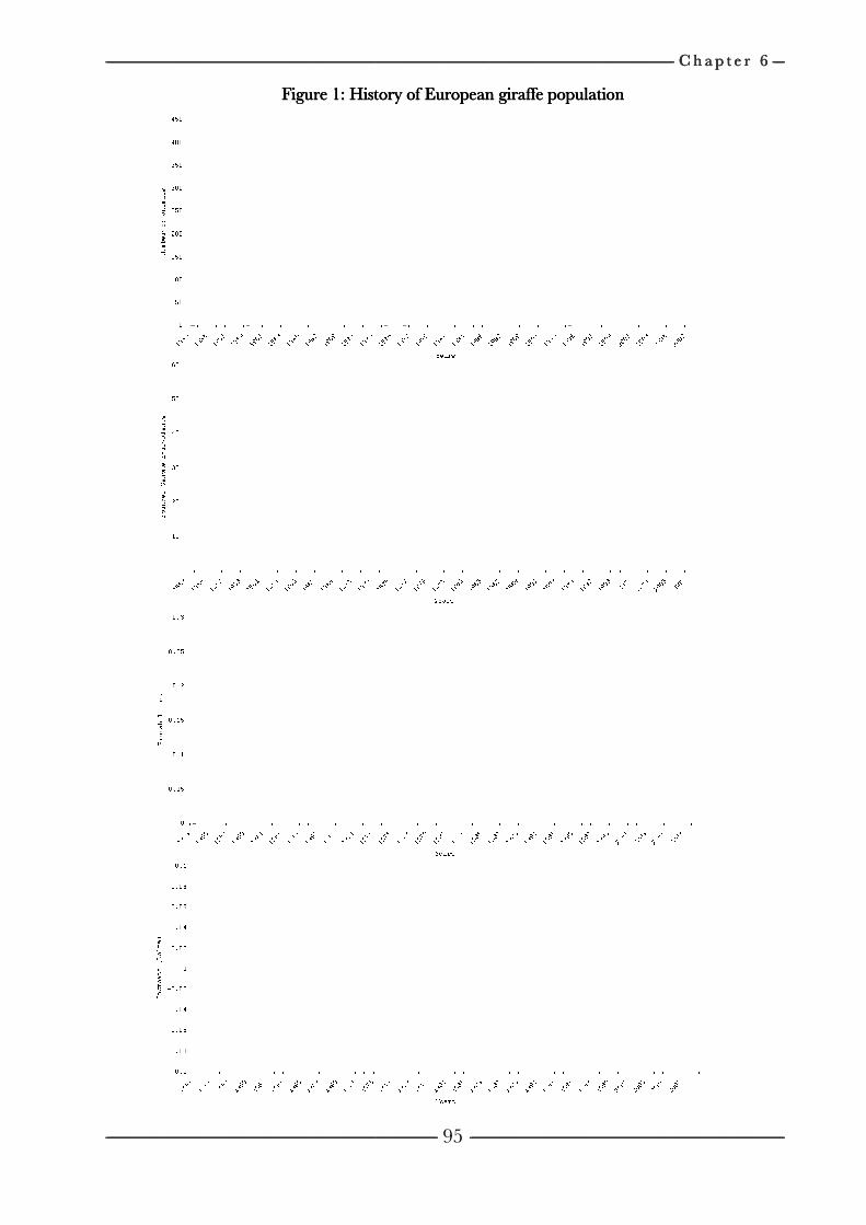
--------------------------------------------------------------------------------------------------------------------------------------------------------------------------------------------------------------------------------------------------------------------------------------------------------------------------------------------------------------------------------------------------------------------------------------------------------------------------------------------------------------------
--------------------------------------------------------------------------------------------------------------------------------------------------------------------------------------------------------------------------------------------------------------------------------------------------------------------------------------------------------------------------------------------------------------------------------------------------------------------------------------------------------------------
--------------------------------------------------------------------------------------------------------------------------------------------------------------------------------------------------------------------------------------------------------------------------------------------------------------------------------------------------------------------------------------------------------------------------------------------------------------------------------------------------------------------
--------------------------------------------------------------------------------------------------------------------------------------------------------------------------------------------------------------------------------------------------------------------------------------------------------------------------------------------------------------------------------------------------------------------------------------------------------------------------------------------------------------------
--------------------------------------------------------------------------------------------------------------------------------------------------------------------------------------------------------------------------------------------------------------------------------------------------------------------------------------------------------------------------------------------------------------------------------------------------------------------------------------------------------------------
--------------------------------------------------------------------------------------------------------------------------------------------------------------------------------------------------------------------------------------------------------------------------------------------------------------------------------------------------------------------------------------------------------------------------------------------------------------------------------------------------------------------
Figure 1: History of European Figure 1: History of European Figure 1: History of European Figure 1: History of European
----------------------------------------------------------------------------------------------------------------------------------------------------------------------------------------------------------------------------------------------------------------------------------------------------------------------------------------------------------------------------------------------------------------------------------------------------------------------------------------------------------------------------------------------------------------------------------------------------------------------------------------------------------------------------------------------------------------------------------------------------------------------------------------
----------------------------------------------------------------------------------------------------------------------------------------------------------------------------------------------------------------------------------------------------------------------------------------------------------------------------------------------------------------------------------------------------------------------------------------------------------------------------------------------------------------------------------------------------------------------------------------------------------------------------------------
Figure 1: History of European Figure 1: History of European Figure 1: History of European Figure 1: History of European
--------------------------------------------------------------------------------------------------------------------------------------------------------------------------------------------------------------------------------------------------------------------
------------------------------------------------------------------------------------------------------------ --------------------------------------------------------------------------------------------------------------------------------------------------------------------------------------------------------------------------------------------------------------------------------------------------------------------------------------------------------------------------------------------------------------------------------------------------------------------------------------------------------------------95
Figure 1: History of European Figure 1: History of European Figure 1: History of European Figure 1: History of European
----------------------------------------------------------------------------------------------------------------------------------------------------------------------------------------------------------------------------------------------------------------------------------------------------------------------------------------------------------------------------------------------------------------------------------------------------------------------------------------------------------------------------------------------------------------------------
--------------------------------------------------------------------------------------------------------------------------------------------------------------------------------------------------------------------------------------------------------------------------------------------------------------------------------------------------------------------------------------------------------------------------------------------------------------------------------------------------------------------
Figure 1: History of European Figure 1: History of European Figure 1: History of European Figure 1: History of European ggggiraffe populationiraffe populationiraffe populationiraffe population
--------------------------------------------------------------------------------------------------------------------------------------------------------------------------------------------------------------------------------------------------------------------------------------------------------
--------------------------------------------------------------------------------------------------------------------------------------------------------------------------------------------------------------------------------------------------------------------------------------------------------------------------------------------------------------------------------------------------------------------------------------------------------------------------------------------------------------------
iraffe populationiraffe populationiraffe populationiraffe population
-------------------------------------------------------------------------------------------------------------------------------------------------------------------------------------------------------------------------------------------------------------------------------------------------------- C h a p t e r C h a p t e r C h a p t e r C h a p t e r
--------------------------------------------------------------------------------------------------------------------------------------------------------------------------------------------------------------------------------------------------------------------------------------------------------------------------------------------------------------------------------------------------------------------------------------------------------------------------------------------------------------------
C h a p t e r C h a p t e r C h a p t e r C h a p t e r 6666 --------------------
--------------------------------------------------------------------------------------------------------------------------------------------------------------------------------------------------------------------------------------------------------------------------------------------------------------------------------------------------------------------------------------------------------------------------------------------------------------------------------------------------------------------------------------------------------------------------------------------------------
--------------------
------------------------------------------------------------------------------------
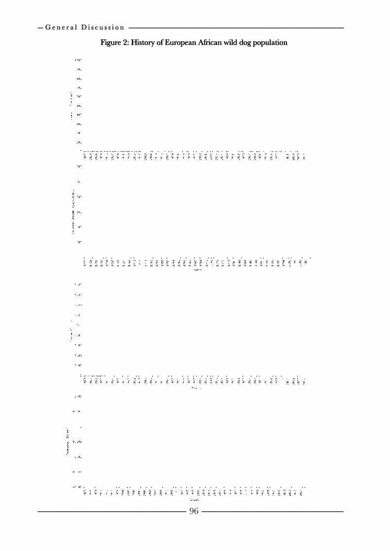
-------------------- G e n e r a l D i s c u s s i o n G e n e r a l D i s c u s s i o n G e n e r a l D i s c u s s i o n G e n e r a l D i s c u s s i o n
----------------------------------------------------------------------------------------------------------------------------------------------------------------------------------------------------------------------------------------------------------------------------------------------------------------------------------------------------------------------------------------------------------------------------------------------------
G e n e r a l D i s c u s s i o n G e n e r a l D i s c u s s i o n G e n e r a l D i s c u s s i o n G e n e r a l D i s c u s s i o n
----------------------------------------------------------------------------------------------------------------------------------------------------------------------------------------------------------------------------------------------------------------------------------------------------------------------------------------------------------------------------------------------------------------------------------------------------
Figure Figure Figure Figure
G e n e r a l D i s c u s s i o n G e n e r a l D i s c u s s i o n G e n e r a l D i s c u s s i o n G e n e r a l D i s c u s s i o n --------------------------------------------------------------------------------------------------------------------------------------------------------------------------------------------------------------------------------------------------------------------------------------------------------------------------------------------------------------------------------------------------------------------------------------------------------------------------------------------------------------------
----------------------------------------------------------------------------------------------------------------------------------------------------------------------------------------------------------------------------------------------------------------------------------------------------------------------------------------------------------------------------------------------------------------------------------------------------
Figure Figure Figure Figure 2222: History of European : History of European : History of European : History of European
--------------------------------------------------------------------------------------------------------------------------------------------------------------------------------------------------------------------------------------------------------------------------------------------------------------------------------------------------------------------------------------------------------------------------------------------------------------------------------------------------------------------
------------------------------------------------------------------------------------------------------------------------------------------------------------------------------------------------------------------------------------------------------------------------------------------------------------------------------------------------------------------------------------------------------------------------------------------------------------------------------------------------------------------------------------------------------------------------------------------------------------
: History of European : History of European : History of European : History of European
--------------------------------------------------------------------------------------------------------------------------------------------------------------------------------------------------------------------------------------------------------------------------------------------------------------------------------------------------------------------------------------------------------------------------------------------------------------------------------------------------------------------
-------------------------------------------------------------------------------------------------------------------------------------------- ------------------------------------------------------------------------------------------------------------------------------------------------------------------------------------------------------------------------96
: History of European : History of European : History of European : History of European African wild dogAfrican wild dogAfrican wild dogAfrican wild dog
--------------------------------------------------------------------------------------------------------------------------------------------------------------------------------------------------------------------------------------------------------------------------------------------------------------------------------------------------------------------------------------------------------------------------------------------------------------------------------------------------------------------
------------------------------------------------------------------------------------------------------------------------------------------------------------------------------------------------------------------------
African wild dogAfrican wild dogAfrican wild dogAfrican wild dog
------------------------------------------------------------------------------------------------------------------------------------------------------------------------------------------------------------------------------------------------------------------------------------------------------------------------------------------------------------------------------------------------------------------------------------------------------------------------------------------------------------------------------------------------------------------------------------------------------------------------------------------------------------------------------------------------------------------------------------------------------------------------------------------------------------------------------------------------------------------------------------------------------------------------
--------------------------------------------------------------------------------------------------------------------------------------------------------------------------------------------------------------------------------------------------------------------------------------------------------------------------------------------------------------------------------------------------------------------------------------------------------------------------------------------------------------------------------------------------------------------------------------------------------
African wild dogAfrican wild dogAfrican wild dogAfrican wild dog populationpopulationpopulationpopulation
----------------------------------------------------------------------------------------------------------------------------------------------------------------------------------------------------------------------------------------------------------------------------------------------------------------------------------------------------------------------------------------------------
----------------------------------------------------------------------------------------------------------------------------------------------------------------------------------------------------------------------------------------------------------------------------------------------------------------------------
populationpopulationpopulationpopulation
----------------------------------------------------------------------------------------------------------------------------------------------------------------------------------------------------------------------------------------------------------------------------------------------------------------------------------------------------------------------------------------------------
----------------------------------------------------------------------------------------------------------------------------------------------------------------------------------------------------------------------------------------------------------------------------------------------------------------------------
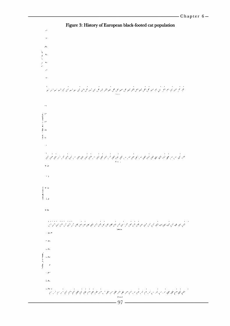
--------------------------------------------------------------------------------------------------------------------------------------------------------------------------------------------------------------------------------------------------------------------------------------------------------------------------------------------------------------------------------------------------------------------------------------------------------------------------------------------------------------------
--------------------------------------------------------------------------------------------------------------------------------------------------------------------------------------------------------------------------------------------------------------------------------------------------------------------------------------------------------------------------------------------------------------------------------------------------------------------------------------------------------------------
--------------------------------------------------------------------------------------------------------------------------------------------------------------------------------------------------------------------------------------------------------------------------------------------------------------------------------------------------------------------------------------------------------------------------------------------------------------------------------------------------------------------
--------------------------------------------------------------------------------------------------------------------------------------------------------------------------------------------------------------------------------------------------------------------------------------------------------------------------------------------------------------------------------------------------------------------------------------------------------------------------------------------------------------------
--------------------------------------------------------------------------------------------------------------------------------------------------------------------------------------------------------------------------------------------------------------------------------------------------------------------------------------------------------------------------------------------------------------------------------------------------------------------------------------------------------------------
--------------------------------------------------------------------------------------------------------------------------------------------------------------------------------------------------------------------------------------------------------------------------------------------------------------------------------------------------------------------------------------------------------------------------------------------------------------------------------------------------------------------
Figure 3: History of European Figure 3: History of European Figure 3: History of European Figure 3: History of European
----------------------------------------------------------------------------------------------------------------------------------------------------------------------------------------------------------------------------------------------------------------------------------------------------------------------------------------------------------------------------------------------------------------------------------------------------------------------------------------------------------------------------------------------------------------------------------------------------------------------------------------------------------------------------------------------------------------------------------------------------------------------------------------
----------------------------------------------------------------------------------------------------------------------------------------------------------------------------------------------------------------------------------------------------------------------------------------------------------------------------------------------------------------------------------------------------------------------------------------------------------------------------------------------------------------------------------------------------------------------------------------------------------------------------------------
Figure 3: History of European Figure 3: History of European Figure 3: History of European Figure 3: History of European
--------------------------------------------------------------------------------------------------------------------------------------------------------------------------------------------------------------------------------------------------------------------
------------------------------------------------------------------------------------------------------------ --------------------------------------------------------------------------------------------------------------------------------------------------------------------------------------------------------------------------------------------------------------------------------------------------------------------------------------------------------------------------------------------------------------------------------------------------------------------------------------------------------------------97
Figure 3: History of European Figure 3: History of European Figure 3: History of European Figure 3: History of European blackblackblackblack
----------------------------------------------------------------------------------------------------------------------------------------------------------------------------------------------------------------------------------------------------------------------------------------------------------------------------------------------------------------------------------------------------------------------------------------------------------------------------------------------------------------------------------------------------------------------------
--------------------------------------------------------------------------------------------------------------------------------------------------------------------------------------------------------------------------------------------------------------------------------------------------------------------------------------------------------------------------------------------------------------------------------------------------------------------------------------------------------------------
blackblackblackblack----footed cat populationfooted cat populationfooted cat populationfooted cat population
--------------------------------------------------------------------------------------------------------------------------------------------------------------------------------------------------------------------------------------------------------------------------------------------------------
--------------------------------------------------------------------------------------------------------------------------------------------------------------------------------------------------------------------------------------------------------------------------------------------------------------------------------------------------------------------------------------------------------------------------------------------------------------------------------------------------------------------
footed cat populationfooted cat populationfooted cat populationfooted cat population
-------------------------------------------------------------------------------------------------------------------------------------------------------------------------------------------------------------------------------------------------------------------------------------------------------- C h a p t e r C h a p t e r C h a p t e r C h a p t e r
--------------------------------------------------------------------------------------------------------------------------------------------------------------------------------------------------------------------------------------------------------------------------------------------------------------------------------------------------------------------------------------------------------------------------------------------------------------------------------------------------------------------
footed cat populationfooted cat populationfooted cat populationfooted cat population
C h a p t e r C h a p t e r C h a p t e r C h a p t e r 6666 --------------------
--------------------------------------------------------------------------------------------------------------------------------------------------------------------------------------------------------------------------------------------------------------------------------------------------------------------------------------------------------------------------------------------------------------------------------------------------------------------------------------------------------------------------------------------------------------------------------------------------------
--------------------
------------------------------------------------------------------------------------
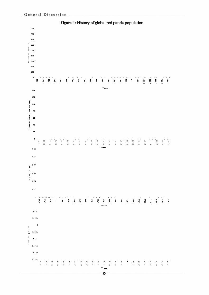
-------------------- G e n e r a l D i s c u s s i o n G e n e r a l D i s c u s s i o n G e n e r a l D i s c u s s i o n G e n e r a l D i s c u s s i o n
----------------------------------------------------------------------------------------------------------------------------------------------------------------------------------------------------------------------------------------------------------------------------------------------------------------------------------------------------------------------------------------------------------------------------------------------------
G e n e r a l D i s c u s s i o n G e n e r a l D i s c u s s i o n G e n e r a l D i s c u s s i o n G e n e r a l D i s c u s s i o n
----------------------------------------------------------------------------------------------------------------------------------------------------------------------------------------------------------------------------------------------------------------------------------------------------------------------------------------------------------------------------------------------------------------------------------------------------
G e n e r a l D i s c u s s i o n G e n e r a l D i s c u s s i o n G e n e r a l D i s c u s s i o n G e n e r a l D i s c u s s i o n --------------------------------------------------------------------------------------------------------------------------------------------------------------------------------------------------------------------------------------------------------------------------------------------------------------------------------------------------------------------------------------------------------------------------------------------------------------------------------------------------------------------
----------------------------------------------------------------------------------------------------------------------------------------------------------------------------------------------------------------------------------------------------------------------------------------------------------------------------------------------------------------------------------------------------------------------------------------------------
Figure 4: History of Figure 4: History of Figure 4: History of Figure 4: History of
--------------------------------------------------------------------------------------------------------------------------------------------------------------------------------------------------------------------------------------------------------------------------------------------------------------------------------------------------------------------------------------------------------------------------------------------------------------------------------------------------------------------
------------------------------------------------------------------------------------------------------------------------------------------------------------------------------------------------------------------------------------------------------------------------------------------------------------------------------------------------------------------------------------------------------------------------------------------------------------------------------------------------------------------------------------------------------------------------------------------------------------
Figure 4: History of Figure 4: History of Figure 4: History of Figure 4: History of
--------------------------------------------------------------------------------------------------------------------------------------------------------------------------------------------------------------------------------------------------------------------------------------------------------------------------------------------------------------------------------------------------------------------------------------------------------------------------------------------------------------------
-------------------------------------------------------------------------------------------------------------------------------------------- ------------------------------------------------------------------------------------------------------------------------------------------------------------------------------------------------------------------------98
Figure 4: History of Figure 4: History of Figure 4: History of Figure 4: History of global red pglobal red pglobal red pglobal red p
--------------------------------------------------------------------------------------------------------------------------------------------------------------------------------------------------------------------------------------------------------------------------------------------------------------------------------------------------------------------------------------------------------------------------------------------------------------------------------------------------------------------
------------------------------------------------------------------------------------------------------------------------------------------------------------------------------------------------------------------------
global red pglobal red pglobal red pglobal red panda populationanda populationanda populationanda population
------------------------------------------------------------------------------------------------------------------------------------------------------------------------------------------------------------------------------------------------------------------------------------------------------------------------------------------------------------------------------------------------------------------------------------------------------------------------------------------------------------------------------------------------------------------------------------------------------------------------------------------------------------------------------------------------------------------------------------------------------------------------------------------------------------------------------------------------------------------------------------------------------------------------
--------------------------------------------------------------------------------------------------------------------------------------------------------------------------------------------------------------------------------------------------------------------------------------------------------------------------------------------------------------------------------------------------------------------------------------------------------------------------------------------------------------------------------------------------------------------------------------------------------
anda populationanda populationanda populationanda population
----------------------------------------------------------------------------------------------------------------------------------------------------------------------------------------------------------------------------------------------------------------------------------------------------------------------------------------------------------------------------------------------------
----------------------------------------------------------------------------------------------------------------------------------------------------------------------------------------------------------------------------------------------------------------------------------------------------------------------------
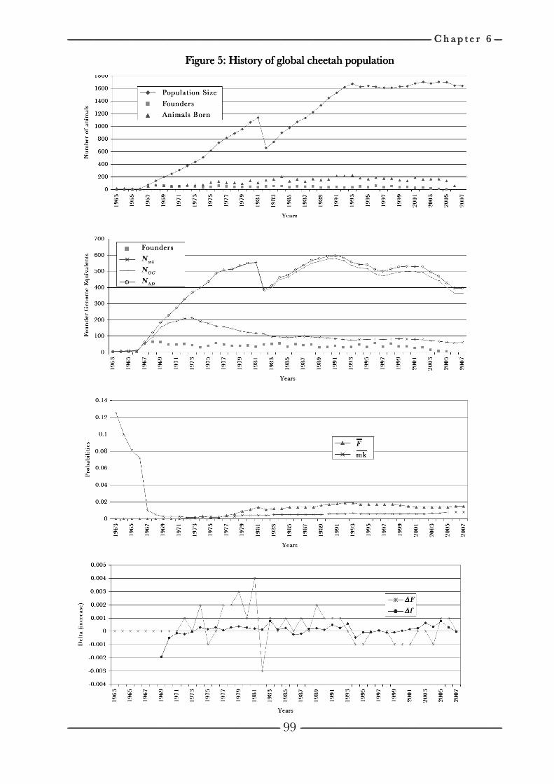
------------------------------------------------------------------------------------------------------------------------------------------------------------------------------------------------------------------------------------------------------------------------------------------------------------------------------------------------------------------------------------------------------------------------------------------------------------------------------------------------------------------------------------------------------------------------------------------------------------------------------------------------------------------------------------------------------------------------------------------------------------------------------------------------------------------------------------------------------------------------------------------------------------------------------------------------------------------------------------------------------------------------------------------------------------------------------------------------ C h a p t e r C h a p t e r C h a p t e r C h a p t e r 6666 --------------------
---------------------------------------------------------------------------------------------------------------------------------------------------------------------------------------------------------------------------------------------------------------------------------------------------------------------------------------------------------------------------------------------------------------------------------------------------------------------------------------------------------------------------------------------------------------------------------------------------------------------------------------- --------------------------------------------------------------------------------------------------------------------------------------------------------------------------------------------------------------------------------------------------------------------------------------------------------------------------------------------------------------------------------------------------------------------------------------------------------------------------------------------------------------------------------------------------------------------------------------------------------
99
Figure 5: History of global Figure 5: History of global Figure 5: History of global Figure 5: History of global ccccheetah populationheetah populationheetah populationheetah population
----------------------------------------------------------------------------------------------------------------------------------------------------------------------------------------------------------------------------------------------------------------------------------------------------------------------------------------------------------------------------------------------------------------------------------------------------------------------------------------------------------------------------------------------------------------------------------------------------------------------------------------------------------------------------------------------------------------------------------------------------------------------------------------------------------------------------------------------------------------------------------------------------------------------------------------------------------------------------------------------------------------------------------------------------------------------------------------------------------------------------------------------------------------------------------------------------------------------------------------------------------------------------------------------------------------
------------------------------------------------------------------------------------------------------------------------------------------------------------------------------------------------------------------------------------------------------------------------------------------------------------------------------------------------------------------------------------------------------------------------------------------------------------------------------------------------------------------------------------------------------------------------------------------------------------------------------------ --------------------------------------------------------------------------------------------------------------------------------------------------------------------------------------------------------------------------------------------------------------------------------------------------------------------------------------------------------------------------------------------------------------------------------------------------------------------------------------------------------------------------------------------------------------------------------------------------------
100
Literature CitedLiterature CitedLiterature CitedLiterature Cited
BALLOU, J.D., and R.C. LACY, 1995199519951995. Identifying genetically important individuals for management of genetic variation in pedigreed populations, pp. 76-111 in Population management for survival and recovery: analytical methods and strategies in small population conservation, edited by J. D. BALLOU, M. E. GILPIN and T. J. FOOSE. New York: Columbia University Press.
BALLOU, J.D., 1997199719971997. Ancestral inbreeding only minimally affects inbreeding depression in mammalian populations. Journal of Heredity 88:88:88:88: 169.
BAUMUNG, R., and J. SÖLKNER, 2003200320032003. Pedigree and marker information requirements to monitor genetic variability. Genetics Selection Evolution 35:35:35:35: 369-383.
BJÖRNERFELDT, S., F. HAILER, M. NORD and C. VILA, 2008200820082008. Assortative mating and fragmentation within dog breeds. BMC Evolutionary Biology 8:8:8:8: 28.
BLOUIN, M.S., 2003200320032003. DNA-based methods for pedigree reconstruction and kinship analysis in natural populations. Trends in Ecology and Evolution 18:18:18:18: 503-511.
BOVENHUIS, H., and J.A. VAN ARENDONK, 1991199119911991. Estimation of milk protein gene frequencies in crossbred cattle by maximum likelihood. Journal of Dairy Science 74:74:74:74: 2728.
BULMER, M.G., 1971197119711971. The effect of selection on genetic variability. American Naturalist 105:105:105:105: 201-211. CABALLERO, A., and M.A. TORO, 2000200020002000. Interrelations between effective population size and other
pedigree tools for the management of conserved populations. Genetical Research 75:75:75:75: 331-343. CLUBB, R., M. ROWCLIFFE, P. LEE, K.U. MAR, C. MOSS and G.J. MASON, 2008200820082008. Compromised
Survivorship in Zoo Elephants. Science 322:322:322:322: 1649. COLE, J.B., 2007200720072007. PyPedal: A computer program for pedigree analysis. Computers and Electronics in
Agriculture 57:57:57:57: 107-113. CRAWFORD, A.M., M.L. TATE, J.C. MCEWAN, G. KUMARAMANICKAVEL, K.M. MCEWAN, K.G.
DODDS, P.A. SWARBRICK and P. THOMPSON, 1993199319931993. How reliable are sheep pedigrees? Proceedings of the New Zealand Society of Animal Production 53:53:53:53: 363-366.
DIAMOND, J.M., 1997199719971997. Guns, Germs, and Steel: The Fates of Human Societies. W.W. Norton & Company, New York.
DIAMOND, J.M., 2005200520052005. Collapse: how societies choose to fail or succeed. Viking, New York. EARNHARDT, J.M., S.D. THOMPSON and K. SCHAD, 2004200420042004. Strategic planning for captive populations:
Projecting changes in genetic diversity. Animal Conservation 7:7:7:7: 9-16. EDING, H., and T.H.E. MEUWISSEN, 2001200120012001. Marker-based estimates of between and within population
kinships for the conservation of genetic diversity. Journal of Animal Breeding and Genetics 118:118:118:118: 141-159.
EDING, H., R. CROOIJMANS, M.A.M. GROENEN and T.H.E. MEUWISSEN, 2002200220022002. Assessing the contribution of breeds to genetic diversity in conservation schemes. Genetics Selection Evolution 34:34:34:34: 613-633.
EDING, H., and T.H.E. MEUWISSEN, 2003200320032003. Linear methods to estimate kinships from genetic marker data for the construction of core sets in genetic conservation schemes. Journal of Animal Breeding and Genetics 120:120:120:120: 289-302.
EID, J., A. FEHR, J. GRAY, K. LUONG, J. LYLE, G. OTTO, P. PELUSO, D. RANK et al., 2008200820082008. Real-Time DNA Sequencing from Single Polymerase Molecules. Science:::: 1162986.
EMIK, L.O., and C.E. TERRILL, 1949194919491949. Systematic Procedures For Calculating Inbreeding Coefficients. Journal of Heredity 40:40:40:40: 51-55.
FALCONER, D.S., and T.F.C. MACKAY, 1996199619961996. Introduction to Quantitative Genetics. Longmans Green, Harlow, Essex, UK.
FAO, 2000200020002000. World Watch List for Domestic Animal Diversity. FAO Publications, Rome. FERNANDEZ, J., M.A. TORO and A. CABALLERO, 2003200320032003. Fixed contributions designs vs. minimization of
global coancestry to control inbreeding in small populations. Genetics 165:165:165:165: 885-894.
----------------------------------------------------------------------------------------------------------------------------------------------------------------------------------------------------------------------------------------------------------------------------------------------------------------------------------------------------------------------------------------------------------------------------------------------------------------------------------------------------------------------------------------------------------------------------------------------------------------------------------------------------------------------------------------------------------------------------------------------------------------------------------------------------------------------------------------------------------------------------------------------------------------------------------------------------------------------------------------------------------------------------------------------------------------------------------------------------------------------------------------------------------------------------------------------------------------------------------------------------------------------------------------------------------------
---------------------------------------------------------------------------------------------------------------------------------------------------------------------------------------------------------------------------------------------------------------------------------------------------------------------------------------------------------------------------------------------------------------------------------------------------------------------------------------------------------------------------------------------------------------------------------------------------------------------------------------- --------------------------------------------------------------------------------------------------------------------------------------------------------------------------------------------------------------------------------------------------------------------------------------------------------------------------------------------------------------------------------------------------------------------------------------------------------------------------------------------------------------------------------------------------------------------------------------------------------
101
FERNANDEZ, J., B. VILLANUEVA, R. PONG-WONG and M.A. TORO, 2005200520052005. Efficiency of the Use of Pedigree and Molecular Marker Information in Conservation Programs. Genetics 170:170:170:170: 1313-1321.
FISHER, R.A., 1958195819581958. The genetical theory of natural selection. Dover Publ., New York. FRANKHAM, R., J.D. BALLOU and D.A. BRISCOE, 2002200220022002. Introduction to Conservation Genetics.
Cambridge University Press, Cambridge, UK. GODDARD, M., 2008200820082008. Genomic selection: prediction of accuracy and maximisation of long term
response. Genetica. GROENEVELD, E., N.H. TINH, W. KUES and N.T. VIEN, 2008200820082008. A protocol for the cryoconservation of
breeds by low-cost emergency cell banks - a pilot study. animal 2:2:2:2: 1-8. HAMILTON, W.D., 1964196419641964. The genetical evolution of social behaviour. II. Journal of theoretical biology 7:7:7:7:
17-52. HENDERSON, C.R., 1984198419841984. Application of Linear Models in Animal Breeding. University of Guelph,
Guelph, Ontario, Canada. HOFFRAGE, U., S. LINDSEY, R. HERTWIG and G. GIGERENZER, 2000200020002000. Communicating statistical
information. Science 290:290:290:290: 2261. HUNT, T.L., and C.P. LIPO, 2006200620062006. Late Colonization of Easter Island. Science:::: 1121879. ISIC, Icelandic Sheepdog International Committee. http://www.icelanddog.org INGVARSSON, P.K., 2002200220022002. Conservation biology: Lone wolf to the rescue. Nature 420:420:420:420: 472. IPCC, 2007200720072007. Climate Change 2007: Synthesis Report of the Intergovernmental Panel on Climate
Change Fourth Assessment Report, pp. 73. Cambridge University Press, Cambridge and New York.
JACQUARD, A., 1983198319831983. Heritability - One Word, 3 Concepts. Biometrics 39:39:39:39: 465-477. KAVAR, T., G. BREM, F. HABE, J. SÖLKNER and P. DOVC, 2002200220022002. History of Lipizzan horse maternal
lines as revealed by mtDNA analysis. Genetics Selection Evolution 34:34:34:34: 635. KENNY, C., 2005200520052005. Why are we worried about income? Nearly everything that matters is converging.
World Development 33:33:33:33: 1. KINGHORN, B.P., S.A. MESZAROS and R.D. VAGG, 2002200220022002. Dynamic tactical decision systems for animal
breeding, pp. in Proceedings of the 7th World Congress on Genetics Applied to Livestock Production.
LACY, R.C., 1989198919891989. Analysis of founder representation in pedigrees: Founder equivalents and founder genome equivalents. Zoo Biology 8:8:8:8: 111.
LACY, R.C., 1995199519951995. Clarification of genetic terms and their use in the management of captive populations. Zoo Biology 14:14:14:14: 565-577.
LAUGHLIN, A.M., D.F. WALDRON, B.F. CRADDOCK, G.R. ENGDAHL, R.K. DUSEK, J.E. HUSTON, C.J. LUPTON, D.N. UECKERT, T.L. SHAY and N.E. COEKETT, 2003200320032003. Use of DNA markers to determine paternity in a multiple-sire mating flock. Sheep and Goat Research Journal 18:18:18:18: 14-17.
LEROY, G., X. ROGNON, A. VARLET, C. JOFFRIN and E. VERRIER, 2006200620062006. Genetic variability in French dog breeds assessed by pedigree data. Journal of Animal Breeding and Genetics 123:123:123:123: 1-9.
LI, C.C., and D.G. HORVITZ, 1953195319531953. Some methods of estimating the inbreeding coefficient. American Journal of Human Genetics 5:5:5:5: 107-117.
LYNCH, M., 1988198819881988. Estimation of relatedness by DNA fingerprinting. Molecular Biology and Evolution 5:5:5:5: 584-599.
LYNCH, M., and B. WALSH, 1997199719971997. Genetics and Analysis of Quantitative Traits. Sinauer Associates, Sunderland, MA.
LYNCH, M., and B. WALSH, 1998199819981998. Genetics and Analysis of Quantitative Traits. Sinauer Associates, Sunderland, MA.
LYNCH, M., and K. RITLAND, 1999199919991999. Estimation of Pairwise Relatedness With Molecular Markers. Genetics 152:152:152:152: 1753-1766.
-------------------- L i t e r a t u r e C i t e d L i t e r a t u r e C i t e d L i t e r a t u r e C i t e d L i t e r a t u r e C i t e d ----------------------------------------------------------------------------------------------------------------------------------------------------------------------------------------------------------------------------------------------------------------------------------------------------------------------------------------------------------------------------------------------------------------------------------------------------------------------------------------------------------------------------------------------------------------------------------------------------------------------------------------------------------------------------------------------------------------------------------------------------------------------------------------------------------------------------------------------------------------------------------------------------------------------------------------------------------------
------------------------------------------------------------------------------------------------------------------------------------------------------------------------------------------------------------------------------------------------------------------------------------------------------------------------------------------------------------------------------------------------------------------------------------------------------------------------------------------------------------------------------------------------------------------------------------------------------------------------------------ --------------------------------------------------------------------------------------------------------------------------------------------------------------------------------------------------------------------------------------------------------------------------------------------------------------------------------------------------------------------------------------------------------------------------------------------------------------------------------------------------------------------------------------------------------------------------------------------------------
102
MALÉCOT, G., 1948194819481948. Les mathématiques de l'hérédité. Masson, Paris. MANN, C.C., 2005200520052005. 1491: New Revelations of the Americas before Columbus. Knopf, New York. MARKER, L., 2008200820082008. 2006 International Cheetah Studbook, pp. 950. Cheetah Conservation Fund,
Otjiwarongo, Namibia. MEUWISSEN, T.H.E., 1997199719971997. Maximizing the response of selection with a predefined rate of inbreeding.
Journal of Animal Science 75:75:75:75: 934-940. MILLIGAN, B.G., 2003200320032003. Maximum-likelihood estimation of relatedness. Genetics 163:163:163:163: 1153-1167. MUCHA, S., and J.J. WINDIG, 2002002002009999. Accepted for Publication: Effects of incomplete pedigree on genetic
management of the Dutch Landrace goat. Journal of Animal Breeding and Genetics 125125125125. MYERS, N., R.A. MITTERMEIER, C.G. MITTERMEIER, G.A.B. DA FONSECA and J. KENT, 2000200020002000.
Biodiversity hotspots for conservation priorities. Nature 403:403:403:403: 853. NICHOLAS, F.W., and C. SMITH, 1983198319831983. Increased rates of genetic change in dairy cattle by embryo
transfer and splitting. Animal Production 36:36:36:36: 341-353. NIELEN, A.L.J., S. VAN DER BEEK, G.J. UBBINK and B.W. KNOL, 2001200120012001. Population parameters to
compare dog breeds: Differences between five Dutch purebred populations. Veterinary Quarterly 23:23:23:23: 43-49.
NOMURA, T., 2005200520052005. Methods for minimizing the loss of genetic diversity in conserved populations with overlapping generations. Conservation Genetics 6:6:6:6: 655.
OSTRANDER, E.A., and R.K. WAYNE, 2005200520052005. The canine genome. Genome Research 15:15:15:15: 1706-1716. PONG-WONG, R., and J.A. WOOLLIAMS, 2007200720072007. Optimisation of contribution of candidate parents to
maximise genetic gain and restricting inbreeding using semidefinite programming (Open Access publication). Genetics Selection Evolution 39:39:39:39: 3-25.
QUELLER, D.C., and K.F. GOODNIGHT, 1989198919891989. Estimating Relatedness Using Genetic-Markers. Evolution 43:43:43:43: 258-275.
RISCHKOWSKY, B., and D. PILLING, 2007200720072007. The State of the World's Animal Genetic Resources for Food and Agriculture, Rome.
RITLAND, K., 1996199619961996. Estimators for pairwise relatedness and individual inbreeding coefficients. Genetical Research 67:67:67:67: 175-186.
RODRÍGUEZ-RAMILO, S., M. TORO, A. CABALLERO and J. FERNÁNDEZ, 2007200720072007. The accuracy of a heritability estimator using molecular information. Conservation Genetics 8:8:8:8: 1189-1198.
RON, M., R. DOMOCHOVSKY, M. GOLIK, E. SEROUSSI, E. EZRA, C. SHTURMAN and J.I. WELLER, 2003200320032003. Analysis of Vaginal Swabs for Paternity Testing and Marker-Assisted Selection in Cattle. Journal of Dairy Science 86:86:86:86: 1818-1820.
RUDNICK, J., and R. LACY, 2008200820082008. The impact of assumptions about founder relationships on the effectiveness of captive breeding strategies. Conservation Genetics 9:9:9:9: 1439.
SÁNCHEZ, L., P. BIJMA and J.A. WOOLLIAMS, 2003200320032003. Minimizing inbreeding by managing genetic contributions across generations. Genetics 164:164:164:164: 1589-1595.
SANDERS, K., J. BENNEWITZ and E. KALM, 2006200620062006. Wrong and missing sire information affects genetic gain in the Angeln dairy cattle population. Journal of Dairy Science 89:89:89:89: 315.
SCHIPPER, J., J.S. CHANSON, F. CHIOZZA, N.A. COX, M. HOFFMANN, V. KATARIYA, J. LAMOREUX, A.S.L. RODRIGUES et al., 2008200820082008. The Status of the World's Land and Marine Mammals: Diversity, Threat, and Knowledge. Science 322:322:322:322: 225-230.
SMIL, V., 2002200220022002. The Earth's Biosphere: Evolution, Dynamics, and Change. The MIT Press, Cambridge. SNEATH, P.H.A., and R.R. SOKAL, 1973197319731973. Numerical Taxonomy. W. H. Freeman and Company, San
Francisco. SONESSON, A.K., and T.H.E. MEUWISSEN, 2001200120012001. Minimization of rate of inbreeding for small
populations with overlapping generations. Genetical Research 77:77:77:77: 285-292. SPELMAN, R.J., 2002200220022002. Utilisation of molecular information in dairy cattle breeding, pp. 11-17 in
Proceedings of the 7th World Congress on Genetics Applied to Livestock Production.
----------------------------------------------------------------------------------------------------------------------------------------------------------------------------------------------------------------------------------------------------------------------------------------------------------------------------------------------------------------------------------------------------------------------------------------------------------------------------------------------------------------------------------------------------------------------------------------------------------------------------------------------------------------------------------------------------------------------------------------------------------------------------------------------------------------------------------------------------------------------------------------------------------------------------------------------------------------------------------------------------------------------------------------------------------------------------------------------------------------------------------------------------------------------------------------------------------------------------------------------------------------------------------------------------------------
---------------------------------------------------------------------------------------------------------------------------------------------------------------------------------------------------------------------------------------------------------------------------------------------------------------------------------------------------------------------------------------------------------------------------------------------------------------------------------------------------------------------------------------------------------------------------------------------------------------------------------------- --------------------------------------------------------------------------------------------------------------------------------------------------------------------------------------------------------------------------------------------------------------------------------------------------------------------------------------------------------------------------------------------------------------------------------------------------------------------------------------------------------------------------------------------------------------------------------------------------------
103
TORO, M., C. BARRAGAN, C. OVILO, J. RODRIGANEZ, C. RODRIGUEZ and L. SILIO, 2002200220022002. Estimation of coancestry in Iberian pigs using molecular markers. Conservation Genetics 3:3:3:3: 309-320.
TORO, M.A., C. BARRAGAN and C. OVILO, 2003200320032003. Estimation of genetic variability of the founder population in a conservation scheme using microsatellites. Animal Genetics 34:34:34:34: 226-228.
UBBINK, G.J., B.W. KNOL and J. BOUW, 1992199219921992. The relationship between homozygosity and the occurrence of specific diseases in Bouvier Belge des Flandres dogs in The Netherlands. Veterinary Quarterly 14:14:14:14: 137-140.
UBBINK, G.J., J. VAN DE BROEK, H.A.W. HAZEWINKEL and J. ROTHUIZEN, 1998199819981998. Cluster analysis of the genetic heterogeneity and disease distributions in purebred dog populations. Veterinary Record 142:142:142:142: 209-213.
UBBINK, G.J., H.A.W. HAZEWINKEL, J. VAN DE BROEK and J. ROTHUIZEN, 1111999999999999. Familial clustering and risk analysis for fragmented coronoid process and elbow joint incongruity in Bernese Mountain Dogs in The Netherlands. American Journal of Veterinary Research 60:60:60:60: 1082-1087.
UBBINK, G.J., T.S.G.A.M. VAN DEN INGH, V. YUZBASIYAN-GURKAN, E. TESKE, J. VAN DE BROEK and J. ROTHUIZEN, 2000200020002000. Population Dynamics of Inherited Copper Toxicosis in Dutch Bedlington Terriers (1977;1997). Journal of Veterinary Internal Medicine 14:14:14:14: 172-176.
VANRADEN, P.M., 1992199219921992. Accounting for Inbreeding and Crossbreeding in Genetic Evaluation of Large Populations. Journal of Dairy Science 75:75:75:75: 3136-3144.
VISSCHER, P.M., J.A. WOOLLIAMS, D. SMITH and J.L. WILLIAMS, 2002200220022002. Estimation of pedigree errors in the UK dairy population using microsatellite markers and the impact on selection. Journal of Dairy Science 85:85:85:85: 2368.
WANG, J.L., 2002200220022002. An estimator for pairwise relatedness using molecular markers. Genetics 160:160:160:160: 1203-1215.
WANG, S., and W.C. FOOTE, 1990199019901990. Protein polymorphism in sheep pedigree testing. Theriogenology 34:34:34:34: 1079-1085.
WAYNE, R.K., and E.A. OSTRANDER, 2007200720072007. Lessons learned from the dog genome. Trends in Genetics 23:23:23:23: 557-567.
WEI, M., A. CABALLERO and W.G. HILL, 1996199619961996. Selection Response in Finite Populations. Genetics 144:144:144:144: 1961-1974.
WELLER, J.I., E. FELDMESSER, M. GOLIK, I. TAGER-COHEN, R. DOMOCHOVSKY, O. ALUS, E. EZRA and M. RON, 2004200420042004. Factors Affecting Incorrect Paternity Assignment in the Israeli Holstein Population. Journal of Dairy Science 87:87:87:87: 2627-2640.
WILSON, E.O., 1992199219921992. The Diversity of Life. Harvard University Press. WILSON, E.O., 2002200220022002. The future of life. Alfred A. Knopf, New York. WISELY, S., R. SANTYMIRE, T. LIVIERI, S. MUETING and J. HOWARD, 2008200820082008. Genotypic and phenotypic
consequences of reintroduction history in the black-footed ferret (Mustela nigripes). Conservation Genetics 9:9:9:9: 389.
WOOLLIAMS, J.A., 2006200620062006. Design and Evaluations for Managing Genetic Diversity in Breeding Programs, pp. in Proceedings of the 8th World Congress on Genetics Applied to Livestock Production, Belo Horizonte, MG, Brasil.
WOOLLIAMS, J.A., 2007200720072007. Genetic contributions and inbreeding, pp. 147-165 in Utilisation and conservation of farm animal genetic resources, edited by K. OLDENBROEK. Wageningen Academic Publishers, Wageningen.
WRIGHT, S., 1922192219221922. Coefficients of Inbreeding and Relationship. American Naturalist 56:56:56:56: 330-338. WRIGHT, S., 1968,1969,1977,19781968,1969,1977,19781968,1969,1977,19781968,1969,1977,1978. Evolution and the Genetics of Populations. University of Chicago
Press, Chicago. YORK, R., and P. MANCUS, 2007200720072007. Diamond in the Rough: Reflections on Guns, Germs, and Steel.
Human Ecology Review 14:14:14:14: 157-162.
----------------------------------------------------------------------------------------------------------------------------------------------------------------------------------------------------------------------------------------------------------------------------------------------------------------------------------------------------------------------------------------------------------------------------------------------------------------------------------------------------------------------------------------------------------------------------------------------------------------------------------------------------------------------------------------------------------------------------------------------------------------------------------------------------------------------------------------------------------------------------------------------------------------------------------------------------------------------------------------------------------------------------------------------------------------------------------------------------------------------------------------------------------------------------------------------------------------------------------------------------------------------------------------------------------------
------------------------------------------------------------------------------------------------------------------------------------------------------------------------------------------------------------------------------------------------------------------------------------------------------------------------------------------------------------------------------------------------------------------------------------------------------------------------------------------------------------------------------------------------------------------------------------------------------------------------------------ --------------------------------------------------------------------------------------------------------------------------------------------------------------------------------------------------------------------------------------------------------------------------------------------------------------------------------------------------------------------------------------------------------------------------------------------------------------------------------------------------------------------------------------------------------------------------------------------------------
104
SummarySummarySummarySummary
An increasing number of breeds and (sub-)species become endangered,
predominantly because of decreasing population sizes. Small populations are at risk because genetic drift constantly lowers genetic diversity which is not compensated by beneficial mutations and selection. Reduction of genetic diversity is eventually followed by higher levels of inbreeding, which can cause inbreeding depression as well as high incidences for particular heritable recessive diseases. Moreover, genetic diversity within populations is required for and correlated with adaptive capacity. Hence, long term survival of small captive populations depends on breeding management that maintain genetic diversity, especially when the parental wild populations no longer serve as a source of population replacements, or integrity of livestock breeds prohibits crossbreeding.
Minimizing kinship plays a central role in management and breeding decisions. Kinship is the probability that two alleles sampled randomly, one from each animal, are ‘identical by descent’, indicating that they descend from a common ancestor. When pedigrees of populations are known, kinship between individuals can be calculated from the pedigree. When pedigree data is lacking or severely incomplete however, estimates of kinship rely on molecular markers. An important strategy in conservation genetics is the preservation of genetic diversity by minimizing the average mean kinship via the preferential breeding of genetically important (distantly related) animals. This thesis uses two main conservation strategies: (1) mean kinship of an animal is the kinship of that animal with all individuals of the current population (including itself); and (2) optimal contributions give each fertile animal (candidate) a specific contribution for next generations. Optimal contributions calculate contributions per animal so that the weighted average mean kinship among candidates is minimized.
Conservation strategies based on kinship might be less effective in practice than expected from theory. For example, kinship can be calculated backwards to founders or only for few generations. Moreover, pedigrees often contain animals with unknown parents, resulting in gaps in the pedigree. Furthermore, misidentified parents are undetected and influences conservation strategies unnoticed. One option is to correct gaps in the pedigrees. Another option is to use molecular markers to infer kinship, which would also solve misidentified parents. However, even when pedigrees are complete and correct, conservation strategies are not always possible to apply. This thesis investigates consequences of for these problems and possible solutions.
For many populations an optimal approach cannot be applied as a breeding strategy, because there is not one single authority that can decide which animals to select for breeding. These populations can still increase genetic diversity with sub-optimal solutions, for which an overview of genetic diversity within these
----------------------------------------------------------------------------------------------------------------------------------------------------------------------------------------------------------------------------------------------------------------------------------------------------------------------------------------------------------------------------------------------------------------------------------------------------------------------------------------------------------------------------------------------------------------------------------------------------------------------------------------------------------------------------------------------------------------------------------------------------------------------------------------------------------------------------------------------------------------------------------------------------------------------------------------------------------------------------------------------------------------------------------------------------------------------------------------------------------------------------------------------------------------------------------------------------------------------------------------------------------------------------------------------------------------
---------------------------------------------------------------------------------------------------------------------------------------------------------------------------------------------------------------------------------------------------------------------------------------------------------------------------------------------------------------------------------------------------------------------------------------------------------------------------------------------------------------------------------------------------------------------------------------------------------------------------------------- --------------------------------------------------------------------------------------------------------------------------------------------------------------------------------------------------------------------------------------------------------------------------------------------------------------------------------------------------------------------------------------------------------------------------------------------------------------------------------------------------------------------------------------------------------------------------------------------------------
105
populations is needed. Hence, individual breeders need insight in the population structure and in how genetic diversity can be maintained. Hierarchical cluster analysis permits the visualization of hitherto unknown structure of pedigreed populations into separate highly related clusters. Previous research shows that the incidences of dog-breed-specific diseases are often bound to specific clusters. Cluster analysis has been carried out on the global Icelandic Sheepdog population, a sheep-herding breed. Results suggest that kinship-based clustering reveals the distribution of available genetic diversity, similar to strategies as mean kinship.
Chapter 2 also compares kinship calculated up to seven generations as had been done in previous research, with kinship calculated including all generations. Results differ markedly, invalidating recommendations based on previous research. According to results, kinship should always be calculated including all generations and thus founders. This chapter also indicates that founders are relevant in small captive populations.
We used simulations to investigate the effect of errors in pedigrees on minimizing kinship. Chapter 3 investigates the influence of wrong as well as missing pedigree information on possibilities to apply optimal contribution selection by simulating panmictic populations. Chapter 4 investigates different ways to deal with missing pedigree information (gaps in pedigrees). Chapter 4 simulates complete pedigrees from the pedigree obtained from three zoo populations having gaps. Hereafter, different ways to correct for gaps were applied on the original pedigree and compared with the ‘simulated’ complete pedigree. Conclusions on how and when to act upon undetected wrong parentage seems inconsistent with Chapter 3 and 4. Chapter 3 concludes from simulated panmictic populations, that a strategy similar to equal contributions is likely to preserve more genetic diversity than optimal contribution selection would when missing parentage is uncorrected or when wrong parentage exceeds 35%. Chapter 4 shows that optimal contribution selection would increase genetic diversity, despite pedigree errors even with uncorrected unknown parents. The main factor causing the differences between Chapter 3 and 4 is that the three zoo-populations showed potential diversity that is almost twice the genetic diversity, while the difference between genetic diversity and potential diversity in Chapter 3 was very low due to panmixia. Thus, in small captive populations the gain due to the difference between actual and potential genetic diversity outpaces the loss due to undetected wrong parentage. Chapter 3 is consistent with Chapter 4 about how to deal with unknown parents: kinship based on pedigree with unknown parent information should always be corrected. Otherwise, conservation methods will predominantly select animals with unknown parents or their offspring, because they appear unrelated while they are not. Chapter 4 shows that three factors improve correction of kinship for unknown parents: (1) correct by using kinship instead of inbreeding; (2) taking averages of candidate
-------------------- S u m m a r y S u m m a r y S u m m a r y S u m m a r y ----------------------------------------------------------------------------------------------------------------------------------------------------------------------------------------------------------------------------------------------------------------------------------------------------------------------------------------------------------------------------------------------------------------------------------------------------------------------------------------------------------------------------------------------------------------------------------------------------------------------------------------------------------------------------------------------------------------------------------------------------------------------------------------------------------------------------------------------------------------------------------------------------------------------------------------------------------------------------------------------------------------------------------------------------------------------------------------------------
------------------------------------------------------------------------------------------------------------------------------------------------------------------------------------------------------------------------------------------------------------------------------------------------------------------------------------------------------------------------------------------------------------------------------------------------------------------------------------------------------------------------------------------------------------------------------------------------------------------------------------ --------------------------------------------------------------------------------------------------------------------------------------------------------------------------------------------------------------------------------------------------------------------------------------------------------------------------------------------------------------------------------------------------------------------------------------------------------------------------------------------------------------------------------------------------------------------------------------------------------
106
parents instead of random assignment of one candidate parent for each unknown parent; and (3) identify probable parents for animals having and unknown parents and a high contribution to the current population. Correction methods that exclude parts of genomes descending from unknown parents save less genetic diversity, and should only be considered to minimize undesirable introgression, while maximizing genetic diversity. Hence, it is crucial to know which animals are founders. Therefore, pedigree registration should always include whether animals without parents are either true founders or non-founders, however with unknown parents.
Chapter 5 compares different kinship estimators that make use of molecular markers and investigates their ability to preserve genetic diversity. In this chapter new estimators were presented, based on the relationship between coancestry and molecular similarity between individuals. Chapter 5 also makes use of simulations that produce both panmictic and structured populations having both true pedigree and molecular marker data. Hence, kinship estimated from molecular markers is compared with the true kinship calculated from pedigree, using statistical criteria and a diversity criterion that minimized kinship. Again results showed that the population structure matters; it influences the ranking of estimators. An existing estimator based on two-gene and four-gene coefficients of identity performs best in panmictic populations, whereas a new estimator based on coancestry performs best in structured populations. Number of marker alleles and loci did not affect ranking of estimators. Statistical criteria were insufficient to evaluate estimators for their use in conservation programs. The regression coefficient of pedigree kinship on estimated kinship (ß2) was substantially lower than unity for all estimators, causing overestimation of the diversity conserved. A simple correction to achieve ß2 = 1, improves both existing and new estimators. Using kinship estimates with correction, considerably increased diversity in structured populations, but did not do so or even decreased diversity in panmictic populations. Hence, the population structure is relevant for conservation.
This thesis shows that all studied captive populations under study lost most of the genetic diversity that was still present in founders but also that populations could still double their genetic diversity with optimal contributions. For example, Chapter 2 shows that though the base population consisted of 36 founders, current diversity of the Icelandic Sheepdog breed is equal to only 2.2 equally contributing founders with no loss of founder alleles in descendants. Maximum attainable diversity is 4.7, which is unlikely to be achieved in a non-supervised breeding population like the Icelandic Sheepdog. The general discussion adds two global captive breeding populations: the red panda and the cheetah, again showing the same pattern. All small captive populations under study are clearly structured. In contrast to panmictic populations, founders are biological relevant in small captive populations. For these populations, therefore, the founders are an
----------------------------------------------------------------------------------------------------------------------------------------------------------------------------------------------------------------------------------------------------------------------------------------------------------------------------------------------------------------------------------------------------------------------------------------------------------------------------------------------------------------------------------------------------------------------------------------------------------------------------------------------------------------------------------------------------------------------------------------------------------------------------------------------------------------------------------------------------------------------------------------------------------------------------------------------------------------------------------------------------------------------------------------------------------------------------------------------------------------------------------------------------------------------------------------------------------------------------------------------------------------------------------------------------------------
---------------------------------------------------------------------------------------------------------------------------------------------------------------------------------------------------------------------------------------------------------------------------------------------------------------------------------------------------------------------------------------------------------------------------------------------------------------------------------------------------------------------------------------------------------------------------------------------------------------------------------------- --------------------------------------------------------------------------------------------------------------------------------------------------------------------------------------------------------------------------------------------------------------------------------------------------------------------------------------------------------------------------------------------------------------------------------------------------------------------------------------------------------------------------------------------------------------------------------------------------------
107
obvious choice as base population and genetic diversity relative to those founders is meaningful. Based on diversity measures for populations under study, this thesis suggests that averages or rates of inbreeding or kinship do not reflect either loss or potential gain of genetic diversity in small captive populations. In conclusion, small captive populations, it is highly beneficial to apply optimal contribution selection, since they are structured. Though deviations of observed kinship from true kinship decreases possibilities to maximize genetic diversity, this can partly be corrected.
----------------------------------------------------------------------------------------------------------------------------------------------------------------------------------------------------------------------------------------------------------------------------------------------------------------------------------------------------------------------------------------------------------------------------------------------------------------------------------------------------------------------------------------------------------------------------------------------------------------------------------------------------------------------------------------------------------------------------------------------------------------------------------------------------------------------------------------------------------------------------------------------------------------------------------------------------------------------------------------------------------------------------------------------------------------------------------------------------------------------------------------------------------------------------------------------------------------------------------------------------------------------------------------------------------------
------------------------------------------------------------------------------------------------------------------------------------------------------------------------------------------------------------------------------------------------------------------------------------------------------------------------------------------------------------------------------------------------------------------------------------------------------------------------------------------------------------------------------------------------------------------------------------------------------------------------------------ --------------------------------------------------------------------------------------------------------------------------------------------------------------------------------------------------------------------------------------------------------------------------------------------------------------------------------------------------------------------------------------------------------------------------------------------------------------------------------------------------------------------------------------------------------------------------------------------------------
108
SSSSAMENVATTINGAMENVATTINGAMENVATTINGAMENVATTING Door een groeiende wereldbevolking worden steeds meer soorten bedreigd. Als
een populatie in aantal afneemt, neemt tevens de genetische diversiteit van die soort af. Dit leidt onvermijdelijk tot een toename van inteelt, hetgeen op zichzelf inteelt depressie kan veroorzaken.. Nog belangrijker, zo’n soort verliest het vermogen zich aan te passen aan veranderende omstandigheden. Dus voor het voortbestaan op de lange termijn van diersoorten en ook huisdierrassen is het noodzakelijk om genetische diversiteit te behouden
Het verlagen van verwantschap (kinship) tussen dieren speelt een belangrijke rol in behoud van populaties. Verwantschap wordt gedefinieerd als de kans tussen nul en één dat twee willekeurige gekozen allelen van twee dieren identiek zijn doordat dat deze dieren van dezelfde voorouder afstammen. Deze verwantschap wordt berekend met behulp van de stamboom. Als de kwaliteit hiervan niet voldoende is kan verwantschap ook worden berekend aan de hand van moleculaire merkers. De belangrijkste strategie voor behoud van genetische diversiteit binnen een populatie is het minimaliseren van de gemiddelde verwantschap in de populatie door het inzetten van genetisch belangrijke dieren in de fokkerij. In dit proefschrift komen voornamelijk twee methoden voor: ‘geoptimaliseerde contributies’ en ‘mean kinship’ waarmee de gemiddelde verwantschap van een dier met de populatie als geheel wordt bedoeld. Optimale contributies zijn contributies per dier welke de gewogen gemiddelde verwantschap (inclusief verwantschap van dieren met zichzelf) minimaliseert. Grofweg berekent optimale contributies per dier het aantal nakomelingen dat ervoor zou zorgen dat in toekomstige generaties de genetische diversiteit maximaal is.
Methoden die genetische diversiteit behouden zouden wel eens minder effectief kunnen zijn in de praktijk dan wat je theoretisch zou verwachten. Als verwantschap bijvoorbeeld wordt gebaseerd op berekeningen die niet verder teruggaan dan zeven generaties (in plaats van tot aan de eerste voorouders ofwel founders) kan dit invloed hebben. Bovendien kunnen er fouten in stambomen voorkomen of zijn ze niet volledig. Dit proefschrift onderzoekt de gevolgen van dit soort fouten op het uiteindelijke behoud van genetische diversiteit. Ook werden oplossingen onderzocht, zoals het corrigeren van missende stamboomgegevens.
In veel gevallen kunnen optimale contributies niet (direct) worden toegepast op populaties die bedreigd zijn, omdat er niet één organisatie/persoon is die kan beslissen over de gehele populatie. Voor veel rassen beslissen individuele fokkers welke dieren ingezet worden. Om in deze gevallen toch diversiteit te behouden is het van belang inzichtelijk te maken waar deze diversiteit gezocht moet worden. Een cluster-analyse op verwantschap voorziet in dit overzicht, omdat zo’n analyse een populatie kan onderverdelen in verwante familie groepen. Binnen dit proefschrift is deze methode toegepast op de IJslandse Hond, een
----------------------------------------------------------------------------------------------------------------------------------------------------------------------------------------------------------------------------------------------------------------------------------------------------------------------------------------------------------------------------------------------------------------------------------------------------------------------------------------------------------------------------------------------------------------------------------------------------------------------------------------------------------------------------------------------------------------------------------------------------------------------------------------------------------------------------------------------------------------------------------------------------------------------------------------------------------------------------------------------------------------------------------------------------------------------------------------------------------------------------------------------------------------------------------------------------------------------------------------------------------------------------------------------------------------
---------------------------------------------------------------------------------------------------------------------------------------------------------------------------------------------------------------------------------------------------------------------------------------------------------------------------------------------------------------------------------------------------------------------------------------------------------------------------------------------------------------------------------------------------------------------------------------------------------------------------------------- --------------------------------------------------------------------------------------------------------------------------------------------------------------------------------------------------------------------------------------------------------------------------------------------------------------------------------------------------------------------------------------------------------------------------------------------------------------------------------------------------------------------------------------------------------------------------------------------------------
109
herdershondenras. Resultaten laten zien dat een cluster-analyse inderdaad inzicht geeft in de populatie structuur.
Dezelfde populatie is gebruikt om een vergelijking te maken tussen verwantschap die werd berekend op enkel zeven generaties vergeleken met een berekening met daarin alle informatie tot aan de eerste voorouders. Volgens de resultaten moet verwantschap altijd berekend worden tot aan de oorspronkelijk voorouders.
Simulatie studies werden gebruikt om de invloed te onderzoeken van fouten in stambomen, met name op het minimaliseren van de gemiddelde verwantschap. In hoofdstuk 3 werd zowel de invloed van missende stamboomgegevens als ongedetecteerde foutieve ouders onderzocht en wel op panmictische populaties (populaties waar willekeurige paring wordt toegepast). In hoofdstuk 4 werden volledige stambomen gesimuleerd vanuit bestaande stambomen van drie dierentuin populaties. In de stambomen van deze populaties kwamen veel onbekende ouders voor. Het is bekend dat als optimale contributies worden toegepast zonder hier iets aan te doen, de genetisch diversiteit mogelijk zelfs terug kan lopen, omdat dieren met onbekende ouders onverwant lijken terwijl ze dat in feite niet zijn. Vervolgens werd gekeken naar verschillende methoden om te corrigeren voor ‘gaten’ in deze stambomen. Drie factoren verbeterden correcties op onbekende ouders: (1) het gebruik van verwantschap tussen mogelijke ouders in plaats van inteelt van deze ouders; (2) het gebruik van gemiddelden in plaats van het willekeurig aanwijzen van één ouder per onbekende ouder en (3) het identificeren van de meest waarschijnlijke ouders voor dieren met onbekende ouders die de grootste bijdrage hebben geleverd aan de huidige generatie. Twee methodes corrigeerden door het uitsluiten van dieren die afstammen van onbekende ouders. Dit had nadelige invloed op behoud van genetische diversiteit en zou daarom alleen toegepast moeten worden als het belang van integriteit van (onder-) soorten of raszuiverheid groter is dan het behoud van adaptief vermogen of het vermijden van inteelt depressie. Verder is het van groot belang dat in stamboeken goed wordt bijgehouden welke dieren de daadwerkelijke ‘founders’ (aan elkaar onverwante oorspronkelijke voorouders) zijn van de populaties.
In hoofdstuk 5 worden verschillende verwantschapschattingsmethoden (schatters) vergeleken die moleculaire merkers gebruiken om verwantschap te berekenen. In dit hoofdstuk worden nieuwe schatters en bestaande schatters vergeleken in het vermogen om de diversiteit in een populatie te verhogen. In hoofdstuk 5 worden zowel panmictische als afwijkende populatie structuren gesimuleerd. Ook hier blijkt dat de populatie structuur invloed heeft op de resultaten. Een bestaande schatter is beter geschikt voor panmictische populaties terwijl een nieuwe schatter beter in staat is om diversiteit te behouden binnen populaties die een groter verschil hebben tussen de huidige genetische diversiteit en de potentiële genetisch diversiteit. Dit verschil tussen potentiële diversiteit en de
-------------------- S a m e n v a t t i n g S a m e n v a t t i n g S a m e n v a t t i n g S a m e n v a t t i n g ------------------------------------------------------------------------------------------------------------------------------------------------------------------------------------------------------------------------------------------------------------------------------------------------------------------------------------------------------------------------------------------------------------------------------------------------------------------------------------------------------------------------------------------------------------------------------------------------------------------------------------------------------------------------------------------------------------------------------------------------------------------------------------------------------------------------------------------------------------------------------------------------------------------------------------------------------------------------------------------------------------------------
------------------------------------------------------------------------------------------------------------------------------------------------------------------------------------------------------------------------------------------------------------------------------------------------------------------------------------------------------------------------------------------------------------------------------------------------------------------------------------------------------------------------------------------------------------------------------------------------------------------------------------ --------------------------------------------------------------------------------------------------------------------------------------------------------------------------------------------------------------------------------------------------------------------------------------------------------------------------------------------------------------------------------------------------------------------------------------------------------------------------------------------------------------------------------------------------------------------------------------------------------
110
huidige diversiteit van een populatie is namelijk vaak veel groter in populaties die met uitsterven bedreigd zijn of risico lopen doordat de populatie in omvang afneemt. Het aantal allelen had geen invloed op de volgorde in prestatie van de schatters. Statistische criteria gaven geen goede indicatie hoe effectief verschillende schatters waren in het behouden van genetische diversiteit. De regressie van de werkelijke verwantschap op de geschatte verwantschap was lager dan één, hetgeen aanduidt dat de genetische diversiteit binnen een populatie wordt overschat. Een simpele correctie-methode die deze regressie terugbrengt tot één verbeterde de prestaties van alle schatters.
Dit proefschrift laat zien dat alle bestudeerde populaties veel genetische diversiteit verloren hebben, zeker ten opzichte van de oorspronkelijke voorouders (zoals wildvang-dieren voor wilde soorten in gevangenschap). De IJslandse Hond bijvoorbeeld beschikte over 36 ‘founders’, maar de huidige genetische diversiteit is vergelijkbaar met die van een populatie die gestart zou worden met 2.2 founders (zonder verlies van allelen). Met een optimaal fok beleid zou dit aantal ‘founder genome equivalents’ verhoogd kunnen worden van 2.2 tot 4.7. In de praktijk is dit echter niet haalbaar omdat dan alleen met specifieke honden gefokt zou moeten worden, terwijl andere dieren helemaal niet meer gebruikt zouden moeten worden. In de algemene discussie (General Discussion: Chapter 6) worden twee populaties in gevangenschap toegevoegd, te weten de gehele jachtluipaarden populatie en de kleine panda. Alle bestudeerde populaties laten zien dat er een duidelijke populatie structuur aanwezig is die sterk afwijkt van een panmictische populatie. Voor dit soort populaties hebben de founders (wildvang-dieren of voor rassen, door oorspronkelijke voorouders die het ras zijn gestart) een ‘biologische’ betekenis. Er zal namelijk bijna nooit meer diversiteit aanwezig zijn in de populatie dan aanwezig was in deze founders.
Voor bedreigde populaties zijn deze founders een logische keuze om alle berekeningen en methoden voor behoud op te baseren. Het heeft vervolgens de voorkeur om de genetische diversiteit van de huidige populatie te vergelijken met de diversiteit die oorspronkelijk aanwezig was (de founders). De veelvuldig gebruikelijke maten voor diversiteit, te weten effectieve populatie grootte en toename van inteelt gaven niet weergeven in welke mate potentiële diversiteit verloren gaat en lijken onvoldoende om de diversiteit in kaart te brengen van populaties die bedreigd zijn.
Bedreigde populaties in gevangenschap kunnen veel voordeel behalen bij het toepassen van optimale contributies, met name omdat er een groot verschil is tussen de potentiële genetische diversiteit en de huidige genetische diversiteit. Voor afwijkingen in de geschatte of berekende verwantschap op de werkelijke verwantschap kan gedeeltelijk gecorrigeerd.
----------------------------------------------------------------------------------------------------------------------------------------------------------------------------------------------------------------------------------------------------------------------------------------------------------------------------------------------------------------------------------------------------------------------------------------------------------------------------------------------------------------------------------------------------------------------------------------------------------------------------------------------------------------------------------------------------------------------------------------------------------------------------------------------------------------------------------------------------------------------------------------------------------------------------------------------------------------------------------------------------------------------------------------------------------------------------------------------------------------------------------------------------------------------------------------------------------------------------------------------------------------------------------------------------------------
---------------------------------------------------------------------------------------------------------------------------------------------------------------------------------------------------------------------------------------------------------------------------------------------------------------------------------------------------------------------------------------------------------------------------------------------------------------------------------------------------------------------------------------------------------------------------------------------------------------------------------------- --------------------------------------------------------------------------------------------------------------------------------------------------------------------------------------------------------------------------------------------------------------------------------------------------------------------------------------------------------------------------------------------------------------------------------------------------------------------------------------------------------------------------------------------------------------------------------------------------------
111
CCCCurriculum Vitaeurriculum Vitaeurriculum Vitaeurriculum Vitae
Ik, Pieter (Petrus Antonius) Oliehoek ben geboren op 15 augustus 1973 te Stompwijk bij mijn ouders Anton Oliehoek en Maria Janssen. Tijdens mijn studie biologie in Wageningen heb ik twee zelf bedachte stages uitgevoerd met als onderwerp karakterising en behoud van (honden-)rassen. Na voltooiing van mijn studie biologie in 1999, ben ik werkzaam geweest in de ICT detacherings branche (Caesar Groep), waar ik ervaring opdeed met vrijwel alle aspecten van software-ontwikkeling. In 2003 besloot ik terug te gaan naar mijn deugd: (onderzoek naar) behoud van dierpopulaties die met uitsterven bedreigd zijn. Het resultaat, daar leest u momenteel in. Naast mijn werk heb ik tevens een basisschool voor natuurlijk leren opgericht (www.natuurlijkleren.net). Ik ben vader van Tijmen en Simon Oliehoek en heb een duurzame relatie met Ziza (Ana Luísa Guimarães Dias) Lourenço.
DankwoordDankwoordDankwoordDankwoord
Allereerst wil ik iedereen; collega's/vrienden/familie/kennisen bedanken voor de inspiratie, gezelligheid en discussies, welke me de energie hebben gegeven dit af te ronden. Mama en Anneke, bedankt mijn steunpilaren te zijn. Papa van jou heb ik die liefde voor (zeldzame) huisdierrassen en diersoorten aangeleerd (of geërft). Michèl, bedankt dat je me geleerd hebt om te kiezen voor wat ik wil: dat was dit onderzoek. Piter, het is heerlijk om met jou geanimeerd een artikel te schrijven. Johan, bedankt voor telkens de kern van een onderzoek eruit te lichten, ook bedankt voor alle vertrouwen die ik (soms schijnbaar tegen beter weten in) genoten heb. Sipke Joost, bedankt voor de boeiende discussies en onophoudelijke motivatie en positieve feedback ook in slechte tijden. Jack bedankt voor alle nuttige commentaren. Saeed thanks for your company as great roommate for so many years. Andreia, many thanks for taking over Saeeds place and all the support, critics and listening. Arie, superbedankt voor het mij-erdoorheen-slepen toen ik echt helemaal aan de grond zat met dit proefschrift. Special thanks to Laurie Marker for allowing me to add cheetah to this thesis. Op de achtergrond is Guus nog altijd aanwezig met het vertrouwen dat hij had dat mijn voor hem onvoorspelbare manier van werken mij toch zou brengen waar ik nu ben. Ziza, thanks love for always being there, also in absence, and I should also thank this job for meeting you. Mijn kinderen, Tijmen en Simon, jullie hebben me zoveel begrip getoond als ik weer en weer en weer werken moest in de schaarse tijd die ik de afgelopen jaren met jullie heb gehad. De omslag betreft een bewerking van een foto van AfriCat: http://www.africat.org/

----------------------------------------------------------------------------------------------------------------------------------------------------------------------------------------------------------------------------------------------------------------------------------------------------------------------------------------------------------------------------------------------------------------------------------------------------------------------------------------------------------------------------------------------------------------------------------------------------------------------------------------------------------------------------------------------------------------------------------------------------------------------------------------------------------------------------------------------------------------------------------------------------------------------------------------------------------------------------------------------------------------------------------------------------------------------------------------------------------------------------------------------------------------------------------------------------------------------------------------------------------------------------------------------------------------
------------------------------------------------------------------------------------------------------------------------------------------------------------------------------------------------------------------------------------------------------------------------------------------------------------------------------------------------------------------------------------------------------------------------------------------------------------------------------------------------------------------------------------------------------------------------------------------------------------------------------------ --------------------------------------------------------------------------------------------------------------------------------------------------------------------------------------------------------------------------------------------------------------------------------------------------------------------------------------------------------------------------------------------------------------------------------------------------------------------------------------------------------------------------------------------------------------------------------------------------------
112

----------------------------------------------------------------------------------------------------------------------------------------------------------------------------------------------------------------------------------------------------------------------------------------------------------------------------------------------------------------------------------------------------------------------------------------------------------------------------------------------------------------------------------------------------------------------------------------------------------------------------------------------------------------------------------------------------------------------------------------------------------------------------------------------------------------------------------------------------------------------------------------------------------------------------------------------------------------------------------------------------------------------------------------------------------------------------------------------------------------------------------------------------------------------------------------------------------------------------------------------------------------------------------------------------------------
---------------------------------------------------------------------------------------------------------------------------------------------------------------------------------------------------------------------------------------------------------------------------------------------------------------------------------------------------------------------------------------------------------------------------------------------------------------------------------------------------------------------------------------------------------------------------------------------------------------------------------------- --------------------------------------------------------------------------------------------------------------------------------------------------------------------------------------------------------------------------------------------------------------------------------------------------------------------------------------------------------------------------------------------------------------------------------------------------------------------------------------------------------------------------------------------------------------------------------------------------------
113
Dit proefschrift is gedrukt op papier met FSC en EU Eco Label certificaat.
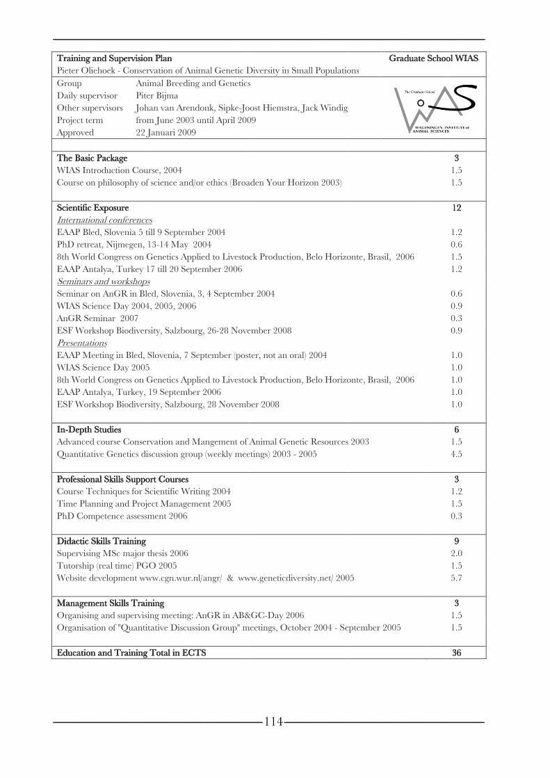
--------------------------------------------------------------------------------------------------------------------------------------------------------------------------------------------------------------------------------------------------------------------------------------------------------------------------------------------------------------------------------------------------------------------------------------------------------------------------------------------------------------------
----------------------------------------------------------------------------------------------------------------------------------------------------------------------------------------------------------------------------------------------------------------------------------------------------------------------------------------------------------------------------------------------------------------------------------------------------
Training and Supervision PlanTraining and Supervision PlanTraining and Supervision PlanTraining and Supervision PlanPieter Oliehoek
Group Daily supervisorOther supervisorsProject termApproved
The Basic PackageThe Basic PackageThe Basic PackageThe Basic PackageWIAS Introduction Course, 2004Course on philosophy of science and/or ethics (Broaden Your Horizon 2003)
Scientific ExposureScientific ExposureScientific ExposureScientific ExposureInternational conferencesEAAP Bled, Slovenia 5 till 9 September 2004PhD retreat, Nijmegen, 138th World Congress on Genetics Applied to Livestock Production, Belo Horizonte, Brasil, 2006EAAP Antalya, Turkey 17 till 20 September 2006Seminars and workshopsSeminar on AnGR in Bled, WIAS Science Day 2004, 2005, 2006AnGR Seminar 2007ESF Workshop Biodiversity, Salzbourg, 26Presentations EAAP Meeting in Bled, Slovenia, 7 September (poster, not an oral) 2004WIAS Science Day 20058th World Congress on Genetics Applied to Livestock Production, Belo Horizonte, Brasil, 2006EAAP Antalya, Turkey, 19 September 2006ESF Workshop Biodiversity, Salzbourg, 28 November 2008
InInInIn----Depth StudiesDepth StudiesDepth StudiesDepth StudiesAdvanced course Conservation and Mangement of Animal Genetic Resources 2003Quantitative Genetics discussion group (weekly meetings) 2003
Professional Skills Support CoursesProfessional Skills Support CoursesProfessional Skills Support CoursesProfessional Skills Support CoursesCourse Techniques for Scientific Writing 2004Time Planning and Project Management 2005PhD Competence assessment 2006
Didactic Skills TrainingDidactic Skills TrainingDidactic Skills TrainingDidactic Skills TrainingSupervising MSc major thesis 2006Tutorship (real time) PGO 2005Website development www.cgn.wur.nl/angr/ &
Management Skills TrainingManagement Skills TrainingManagement Skills TrainingManagement Skills TrainingOrganising and supervising meeting: AnGR in AB&GCOrganisation of "Quantitative Discussion Group" meetings, October 2004
Education and Training Education and Training Education and Training Education and Training
--------------------------------------------------------------------------------------------------------------------------------------------------------------------------------------------------------------------------------------------------------------------------------------------------------------------------------------------------------------------------------------------------------------------------------------------------------------------------------------------------------------------
----------------------------------------------------------------------------------------------------------------------------------------------------------------------------------------------------------------------------------------------------------------------------------------------------------------------------------------------------------------------------------------------------------------------------------------------------
Training and Supervision PlanTraining and Supervision PlanTraining and Supervision PlanTraining and Supervision PlanPieter Oliehoek - Conservation of
Animal Breeding and Genetics Daily supervisor Piter BijmaOther supervisors Johan van Arendonk, SipkeProject term from June 2003 until April 2009
22 Januari 2009
The Basic PackageThe Basic PackageThe Basic PackageThe Basic Package WIAS Introduction Course, 2004Course on philosophy of science and/or ethics (Broaden Your Horizon 2003)
Scientific ExposureScientific ExposureScientific ExposureScientific Exposure International conferencesEAAP Bled, Slovenia 5 till 9 September 2004PhD retreat, Nijmegen, 138th World Congress on Genetics Applied to Livestock Production, Belo Horizonte, Brasil, 2006EAAP Antalya, Turkey 17 till 20 September 2006Seminars and workshopsSeminar on AnGR in Bled, WIAS Science Day 2004, 2005, 2006AnGR Seminar 2007 ESF Workshop Biodiversity, Salzbourg, 26Presentations EAAP Meeting in Bled, Slovenia, 7 September (poster, not an oral) 2004WIAS Science Day 20058th World Congress on Genetics Applied to Livestock Production, Belo Horizonte, Brasil, 2006EAAP Antalya, Turkey, 19 September 2006ESF Workshop Biodiversity, Salzbourg, 28 November 2008
Depth StudiesDepth StudiesDepth StudiesDepth Studies Advanced course Conservation and Mangement of Animal Genetic Resources 2003Quantitative Genetics discussion group (weekly meetings) 2003
Professional Skills Support CoursesProfessional Skills Support CoursesProfessional Skills Support CoursesProfessional Skills Support CoursesCourse Techniques for Scientific Writing 2004
Planning and Project Management 2005PhD Competence assessment 2006
Didactic Skills TrainingDidactic Skills TrainingDidactic Skills TrainingDidactic Skills Training Supervising MSc major thesis 2006Tutorship (real time) PGO 2005Website development www.cgn.wur.nl/angr/ &
Management Skills TrainingManagement Skills TrainingManagement Skills TrainingManagement Skills TrainingOrganising and supervising meeting: AnGR in AB&GCOrganisation of "Quantitative Discussion Group" meetings, October 2004
Education and Training Education and Training Education and Training Education and Training
--------------------------------------------------------------------------------------------------------------------------------------------------------------------------------------------------------------------------------------------------------------------------------------------------------------------------------------------------------------------------------------------------------------------------------------------------------------------------------------------------------------------
----------------------------------------------------------------------------------------------------------------------------------------------------------------------------------------------------------------------------------------------------------------------------------------------------------------------------------------------------------------------------------------------------------------------------------------------------
Training and Supervision PlanTraining and Supervision PlanTraining and Supervision PlanTraining and Supervision Plan Conservation of Animal Genetic Diversity in Small Populations
Animal Breeding and Genetics Piter Bijma Johan van Arendonk, Sipkefrom June 2003 until April 2009
Januari 2009
WIAS Introduction Course, 2004 Course on philosophy of science and/or ethics (Broaden Your Horizon 2003)
International conferences EAAP Bled, Slovenia 5 till 9 September 2004PhD retreat, Nijmegen, 13-14 May 20048th World Congress on Genetics Applied to Livestock Production, Belo Horizonte, Brasil, 2006EAAP Antalya, Turkey 17 till 20 September 2006Seminars and workshops Seminar on AnGR in Bled, Slovenia, 3, 4 September 2004WIAS Science Day 2004, 2005, 2006
ESF Workshop Biodiversity, Salzbourg, 26
EAAP Meeting in Bled, Slovenia, 7 September (poster, not an oral) 2004WIAS Science Day 2005 8th World Congress on Genetics Applied to Livestock Production, Belo Horizonte, Brasil, 2006EAAP Antalya, Turkey, 19 September 2006ESF Workshop Biodiversity, Salzbourg, 28 November 2008
Advanced course Conservation and Mangement of Animal Genetic Resources 2003Quantitative Genetics discussion group (weekly meetings) 2003
Professional Skills Support CoursesProfessional Skills Support CoursesProfessional Skills Support CoursesProfessional Skills Support Courses Course Techniques for Scientific Writing 2004
Planning and Project Management 2005PhD Competence assessment 2006
Supervising MSc major thesis 2006 Tutorship (real time) PGO 2005 Website development www.cgn.wur.nl/angr/ &
Management Skills TrainingManagement Skills TrainingManagement Skills TrainingManagement Skills Training Organising and supervising meeting: AnGR in AB&GCOrganisation of "Quantitative Discussion Group" meetings, October 2004
Education and Training Education and Training Education and Training Education and Training Total in ECTSTotal in ECTSTotal in ECTSTotal in ECTS
----------------------------------------------------------------------------------------------------------------------------------------------------------------------------------------------------------------------------------------------------------------------------------------------------------------------------------------------------------------------------------------------------------------------------------------------------------------------------------------------------------------------------------------------------------------------------------------------------------------------------------------------------------------------------------------------------------------------------------------------------------------------------------------------------------------------------------------------------------------------------------------------------------------------------------------------------------------------------------------------------------------------------------------
------------------------------------------------------------------------------------------------------------------------------------------------------------------------------------------------------------------------------------------------------------------------------------------------------------------------------------------------------------------------------------------------------------------------------------------------------------------------------------------------------------------------------------------------------------------------------------------------------------
Animal Genetic Diversity in Small Populations
Animal Breeding and Genetics
Johan van Arendonk, Sipke-Joost Hiemstra, Jack Windigfrom June 2003 until April 2009
Course on philosophy of science and/or ethics (Broaden Your Horizon 2003)
EAAP Bled, Slovenia 5 till 9 September 2004 14 May 2004
8th World Congress on Genetics Applied to Livestock Production, Belo Horizonte, Brasil, 2006EAAP Antalya, Turkey 17 till 20 September 2006
Slovenia, 3, 4 September 2004
ESF Workshop Biodiversity, Salzbourg, 26-28 November 2008
EAAP Meeting in Bled, Slovenia, 7 September (poster, not an oral) 2004
8th World Congress on Genetics Applied to Livestock Production, Belo Horizonte, Brasil, 2006EAAP Antalya, Turkey, 19 September 2006 ESF Workshop Biodiversity, Salzbourg, 28 November 2008
Advanced course Conservation and Mangement of Animal Genetic Resources 2003Quantitative Genetics discussion group (weekly meetings) 2003
Course Techniques for Scientific Writing 2004 Planning and Project Management 2005
Website development www.cgn.wur.nl/angr/ & www.geneticdiversity.net/ 2005
Organising and supervising meeting: AnGR in AB&GCOrganisation of "Quantitative Discussion Group" meetings, October 2004
Total in ECTSTotal in ECTSTotal in ECTSTotal in ECTS
--------------------------------------------------------------------------------------------------------------------------------------------------------------------------------------------------------------------------------------------------------------------------------------------------------------------------------------------------------------------------------------------------------------------------------------------------------------------------------------------------------------------
-------------------------------------------------------------------------------------------------------------------------------------------- ------------------------------------------------------------------------------------------------------------------------------------------------------------------------------------------------------------------------114
Animal Genetic Diversity in Small Populations
Animal Breeding and Genetics
Joost Hiemstra, Jack Windigfrom June 2003 until April 2009
Course on philosophy of science and/or ethics (Broaden Your Horizon 2003)
8th World Congress on Genetics Applied to Livestock Production, Belo Horizonte, Brasil, 2006
Slovenia, 3, 4 September 2004
28 November 2008
EAAP Meeting in Bled, Slovenia, 7 September (poster, not an oral) 2004
8th World Congress on Genetics Applied to Livestock Production, Belo Horizonte, Brasil, 2006
ESF Workshop Biodiversity, Salzbourg, 28 November 2008
Advanced course Conservation and Mangement of Animal Genetic Resources 2003Quantitative Genetics discussion group (weekly meetings) 2003 -
www.geneticdiversity.net/ 2005
Organising and supervising meeting: AnGR in AB&GC-Day 2006Organisation of "Quantitative Discussion Group" meetings, October 2004
--------------------------------------------------------------------------------------------------------------------------------------------------------------------------------------------------------------------------------------------------------------------------------------------------------------------------------------------------------------------------------------------------------------------------------------------------------------------------------------------------------------------
------------------------------------------------------------------------------------------------------------------------------------------------------------------------------------------------------------------------
Animal Genetic Diversity in Small Populations
Joost Hiemstra, Jack Windig
Course on philosophy of science and/or ethics (Broaden Your Horizon 2003)
8th World Congress on Genetics Applied to Livestock Production, Belo Horizonte, Brasil, 2006
EAAP Meeting in Bled, Slovenia, 7 September (poster, not an oral) 2004
8th World Congress on Genetics Applied to Livestock Production, Belo Horizonte, Brasil, 2006
Advanced course Conservation and Mangement of Animal Genetic Resources 2003 2005
www.geneticdiversity.net/ 2005
Day 2006 Organisation of "Quantitative Discussion Group" meetings, October 2004 - September 2005
--------------------------------------------------------------------------------------------------------------------------------------------------------------------------------------------------------------------------------------------------------------------------------------------------------------------------------------------------------------------------------------------------------------------------------------------------------------------------------------------------------------------------------------------
--------------------------------------------------------------------------------------------------------------------------------------------------------------------------------------------------------------------------------------------------------------------------------------------------------------------------------------------------------------------------------------------------------------------------------------------------------------------------------------------------------------------------------------------------------------------------------------------------------
Graduate School WIASGraduate School WIASGraduate School WIASGraduate School WIASAnimal Genetic Diversity in Small Populations
8th World Congress on Genetics Applied to Livestock Production, Belo Horizonte, Brasil, 2006
8th World Congress on Genetics Applied to Livestock Production, Belo Horizonte, Brasil, 2006
Advanced course Conservation and Mangement of Animal Genetic Resources 2003
www.geneticdiversity.net/ 2005
September 2005
------------------------------------------------------------------------------------------------------------------------------------------------------------------------------------------------------------------------------------------------------------------------
----------------------------------------------------------------------------------------------------------------------------------------------------------------------------------------------------------------------------------------------------------------------------------------------------------------------------
Graduate School WIASGraduate School WIASGraduate School WIASGraduate School WIAS
8th World Congress on Genetics Applied to Livestock Production, Belo Horizonte, Brasil, 2006
8th World Congress on Genetics Applied to Livestock Production, Belo Horizonte, Brasil, 2006
September 2005
------------------------------------------------------------------------------------------------------------------------------------------------------------------------------------------------------------------------------------------------
----------------------------------------------------------------------------------------------------------------------------------------------------------------------------------------------------------------------------------------------------------------------------------------------------------------------------
Graduate School WIASGraduate School WIASGraduate School WIASGraduate School WIAS
3333 1.5 1.5
12121212
1.2 0.6 1.5 1.2
0.6 0.9 0.3 0.9
1.0 1.0 1.0 1.0 1.0
6666 1.5 4.5
3333 1.2 1.5 0.3
9999 2.0 1.5 5.7
3333 1.5 1.5
36363636