Embed Size (px)
Citation preview
Genomic Selection in Tomato Breeding
SolCAP Workshop, Tomato Breeders
Round-Table , Ithaca, NY
David M. Francis, S.C. Sim, Heather Merk The Ohio State University Allen Van Deynze, U.C. Davis C. Robin Buell, J. Hamilton, D. Douches, Michigan State University Walter De Jong, Lucas Mueller, Cornell University
Mathilde Causse Martin Ganal
Acknowledgments:
Discussion Dr. Jean-Luc Jannink, USDA/ARS, Ithaca, NY Dr. Clay Sneller, Dept. Hort. and Crop Science, OSU Resources developed by Dr. Ben Hayes, Dept. of Primary Industries, Victoria, Australia http://www.ans.iastate.edu/section/abg/shortcourse/notes.pdf Dr. Ed Buckler and colleagues, http://www.maizegenetics.net/ Dr. Gustavo de los Campos and colleagues, http://genomics.cimmyt.org/
Overview (1) Association Analysis Identifying significant marker-trait linkages in complex populations (2) Genomic Selection Predicting breeding value of an individual based on kinship and genotype (3) Preparing Data (4) Resources (5) Practical Examples
At the end of this module you will be able to: Describe Association Analysis and Genome Wide Selection (GWS) Define and estimate a Breeding Value Define a multiple trait index Prepare data for AA and GWS Know how to access demonstrations and practical exercises.

Definitions Association Analysis Mapping in unstructured populations Marker Assisted Selection (MAS) Selection based on Marker-QTL linkage Direct selection Selection for coupling-phase recombination Background genome selection for accelerated BC Selection for multiple QTL, etc… Genomic Selection (GWS) Selection based on breeding value Random effects models and BLUPs Estimate breeding value for markers and individuals

Association Analysis Proposed as a way to overcome limitations of working with bi-parental populations for QTL-based discovery and subsequent MAS In complex populations the magnitude of QTL effects tend to be small Relevance of the complex population to applied goals remains an issue (e.g. inbred lines vs hybrids)
Association Analysis Data Vector of trait values from phenotypic evaluation of a large complex population (best if these are BLUPs) Matrix of Markers Matrix of population structure (STRUCTURE or PCA) Kinship matrix
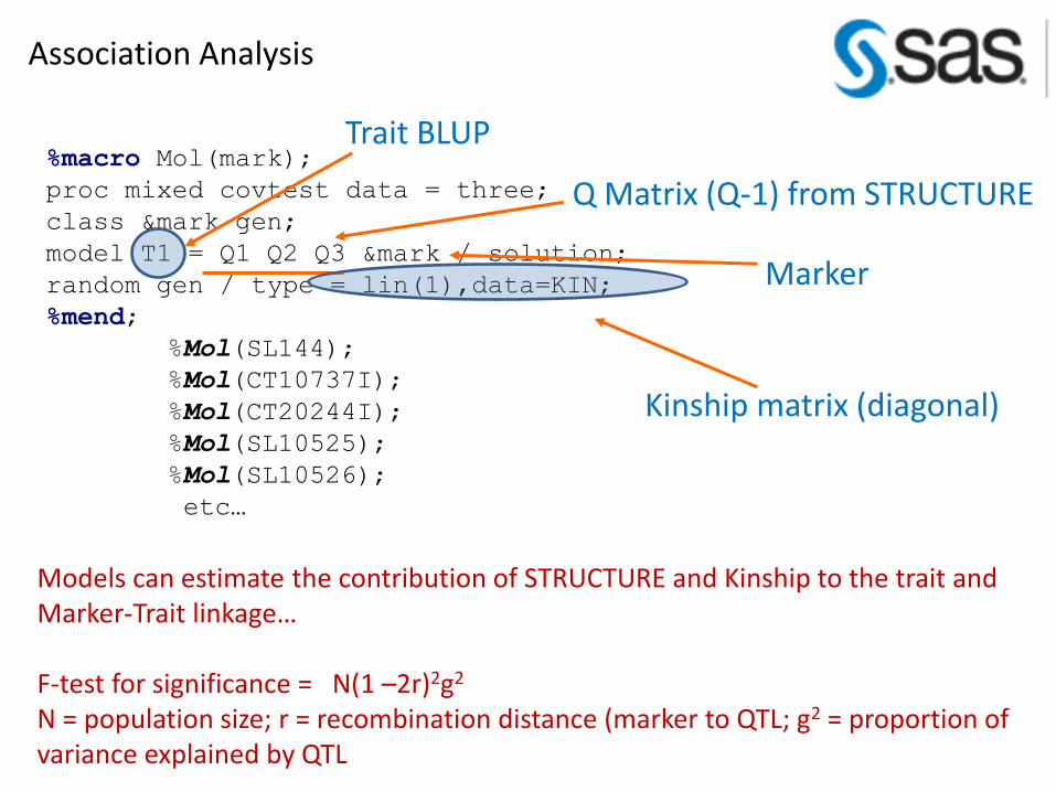
%macro Mol(mark);
proc mixed covtest data = three;
class &mark gen;
model T1 = Q1 Q2 Q3 &mark / solution;
random gen / type = lin(1),data=KIN;
%mend;
%Mol(SL144);
%Mol(CT10737I);
%Mol(CT20244I);
%Mol(SL10525);
%Mol(SL10526);
etc…
Marker
Q Matrix (Q-1) from STRUCTURE
Models can estimate the contribution of STRUCTURE and Kinship to the trait and Marker-Trait linkage… F-test for significance = N(1 –2r)2g2 N = population size; r = recombination distance (marker to QTL; g2 = proportion of variance explained by QTL
Trait BLUP
Association Analysis
Kinship matrix (diagonal)
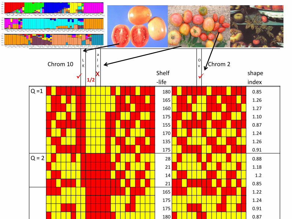
Chrom 10
L
K
a
l
c
O
v Chrom 2
Shelf
-life
shape
index
Q =1 180 0.85
165 1.26
160 1.27
175 1.10
155 0.87
170 1.24
135 1.26
175 0.91
Q = 2 28 0.88
21 1.18
14 1.2
21 0.85
165 1.22
175 1.24
175 0.91
180 0.87
1/2 x
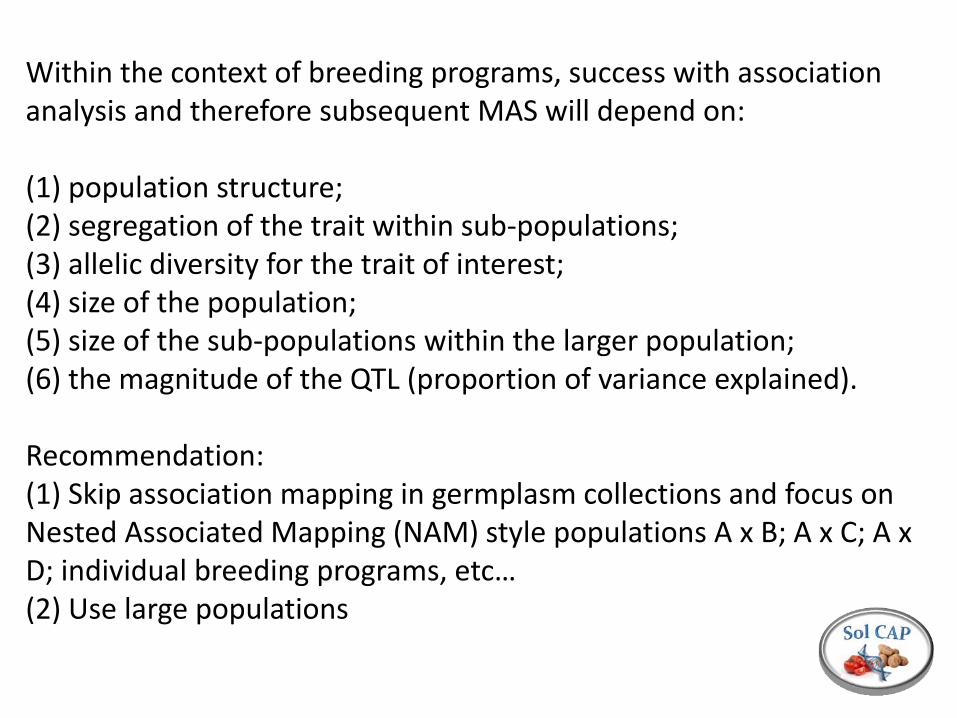
Within the context of breeding programs, success with association analysis and therefore subsequent MAS will depend on: (1) population structure; (2) segregation of the trait within sub-populations; (3) allelic diversity for the trait of interest; (4) size of the population; (5) size of the sub-populations within the larger population; (6) the magnitude of the QTL (proportion of variance explained). Recommendation: (1) Skip association mapping in germplasm collections and focus on Nested Associated Mapping (NAM) style populations A x B; A x C; A x D; individual breeding programs, etc… (2) Use large populations
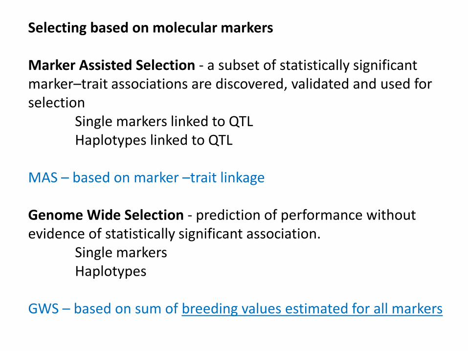
Selecting based on molecular markers Marker Assisted Selection - a subset of statistically significant marker–trait associations are discovered, validated and used for selection Single markers linked to QTL Haplotypes linked to QTL MAS – based on marker –trait linkage Genome Wide Selection - prediction of performance without evidence of statistically significant association. Single markers Haplotypes GWS – based on sum of breeding values estimated for all markers

Genomic selection (GS) Selection decisions based on genomic breeding values estimated as the sum of the effects of markers across the genome (Contrast to MAS in which only markers positively associated with trait are used). Breeding values are derived from Best Linear Unbiased Predictors (BLUPs) as the sum of BLUPs for all markers. Can estimate the breeding value of an individual, even when there are no observations (e.g. Dairy Sire example).
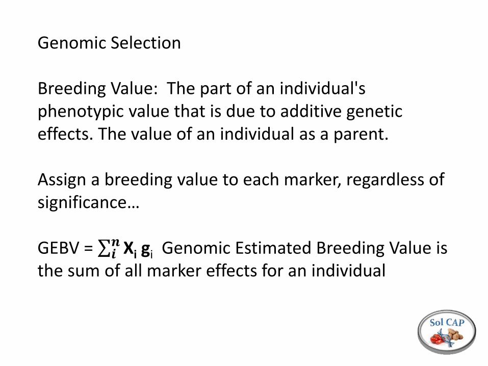
Genomic Selection Breeding Value: The part of an individual's phenotypic value that is due to additive genetic effects. The value of an individual as a parent. Assign a breeding value to each marker, regardless of significance… GEBV = Xi gi
𝒏𝒊 Genomic Estimated Breeding Value is
the sum of all marker effects for an individual
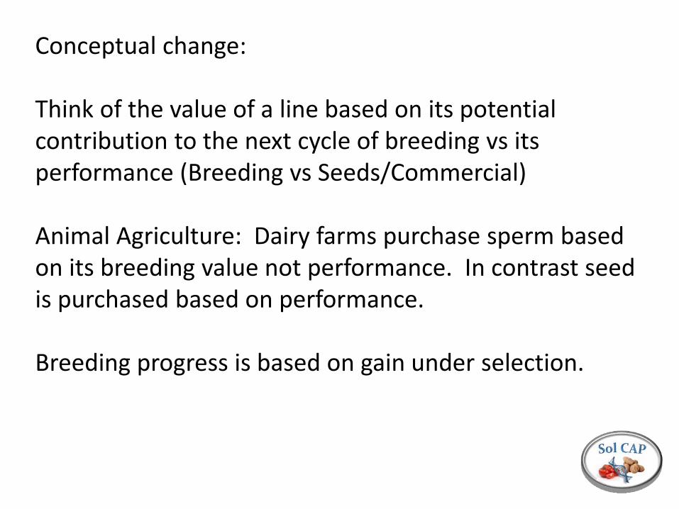
Conceptual change: Think of the value of a line based on its potential contribution to the next cycle of breeding vs its performance (Breeding vs Seeds/Commercial) Animal Agriculture: Dairy farms purchase sperm based on its breeding value not performance. In contrast seed is purchased based on performance. Breeding progress is based on gain under selection.

Implications Significance of Marker-Trait (QTL) association (linkage) is less important than the estimated breeding value We need to start thinking about Marker-QTL linkages as random effects effects (markers) > than phenotypic observations effects are estimated as BLUPs Estimates of breeding value are strengthened by data from relatives, therefore pedigrees, kinship matrices, etc… improve estimates of breeding values.
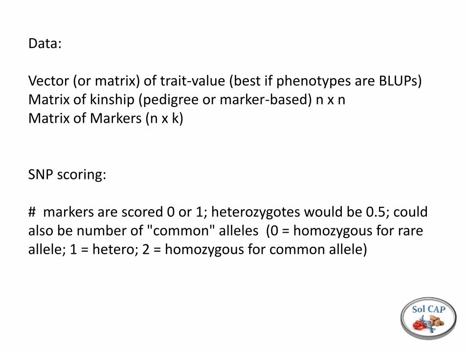
Data: Vector (or matrix) of trait-value (best if phenotypes are BLUPs) Matrix of kinship (pedigree or marker-based) n x n Matrix of Markers (n x k) SNP scoring: # markers are scored 0 or 1; heterozygotes would be 0.5; could also be number of "common" alleles (0 = homozygous for rare allele; 1 = hetero; 2 = homozygous for common allele)
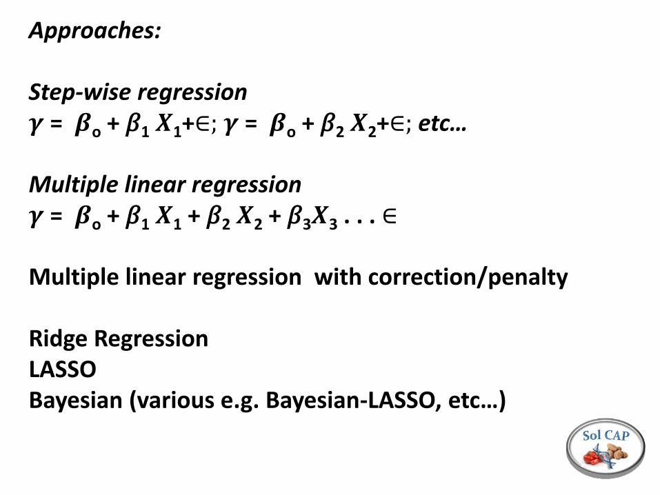
Approaches: Step-wise regression 𝜸 = 𝜷o + 𝛽1 𝑿1+∈; 𝜸 = 𝜷o + 𝛽2 𝑿2+∈; etc… Multiple linear regression 𝜸 = 𝜷o + 𝛽1 𝑿1 + 𝛽2 𝑿2 + 𝛽3𝑿3 . . . ∈ Multiple linear regression with correction/penalty Ridge Regression LASSO Bayesian (various e.g. Bayesian-LASSO, etc…)

Comparing Stepwise with Multiple Regression (statistically naïve thought experiment)
fit1 = lmer(BL_L~(1|M1)) Phenotype Marker ranef(fit1) . . . fit5 = lmer(BL_L~(1|M5)) ranef(fit5) fitML = lmer(BL_L~(1|M1)+(1|M2)+(1|M3)+(1|M4)+(1|M5)) ranef(fitML)
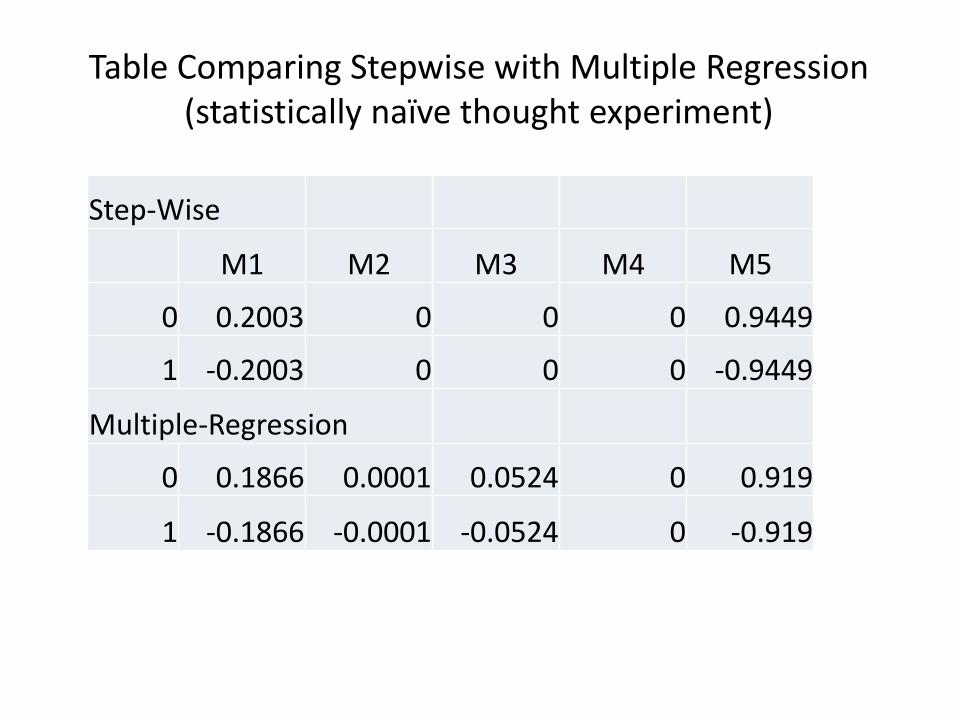
Table Comparing Stepwise with Multiple Regression (statistically naïve thought experiment)
Step-Wise
M1 M2 M3 M4 M5
0 0.2003 0 0 0 0.9449
1 -0.2003 0 0 0 -0.9449
Multiple-Regression
0 0.1866 0.0001 0.0524 0 0.919
1 -0.1866 -0.0001 -0.0524 0 -0.919
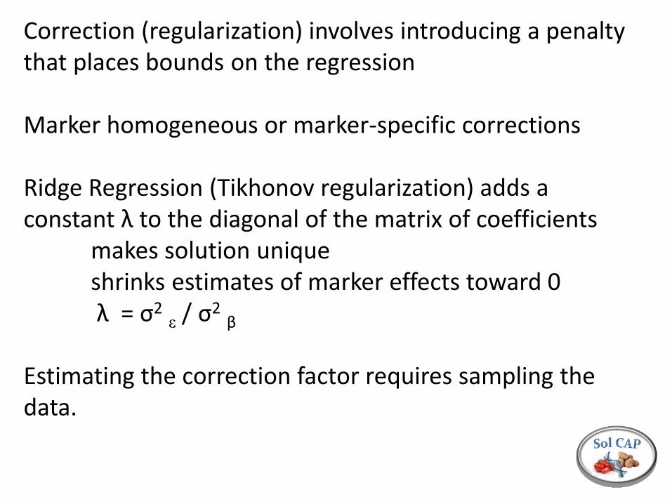
Correction (regularization) involves introducing a penalty that places bounds on the regression
Marker homogeneous or marker-specific corrections Ridge Regression (Tikhonov regularization) adds a constant λ to the diagonal of the matrix of coefficients makes solution unique shrinks estimates of marker effects toward 0 λ = σ2 ε / σ2 β
Estimating the correction factor requires sampling the data.
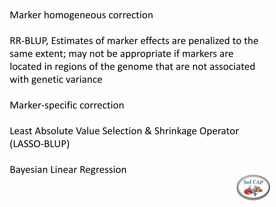
Marker homogeneous correction RR-BLUP, Estimates of marker effects are penalized to the same extent; may not be appropriate if markers are located in regions of the genome that are not associated with genetic variance Marker-specific correction Least Absolute Value Selection & Shrinkage Operator (LASSO-BLUP) Bayesian Linear Regression
Training Population
Phenotype & Genotype
Breeding Material
Genotype Estimate Genomic Breeding Value
Selections
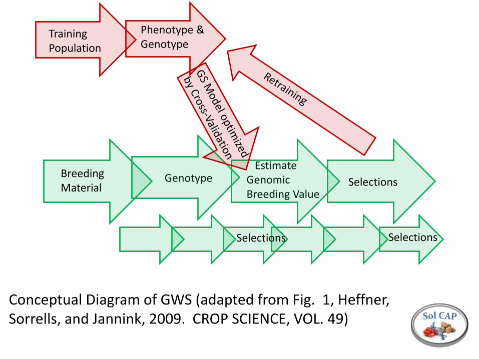
Conceptual Diagram of GWS (adapted from Fig. 1, Heffner, Sorrells, and Jannink, 2009. CROP SCIENCE, VOL. 49)
Selections Selections

Genomic selection is based on a prediction of breeding value Accuracy depends on the size of the training population, number of markers, heritability of the trait, and the number of genes contributing to the trait We can control the population size (and composition) The number of markers is no longer limiting (SolCAP infinium Array, Genotyping by Sequencing, etc…) The process is iterative, with statistical models re-estimated after each cycle of phenotypic evaluation The relative efficiency of GWS will often be lower than direct phenotypic selection; value is to select during rapid generation turn over such that multiple cycles of selection can occur. The issue of what to select for remains…
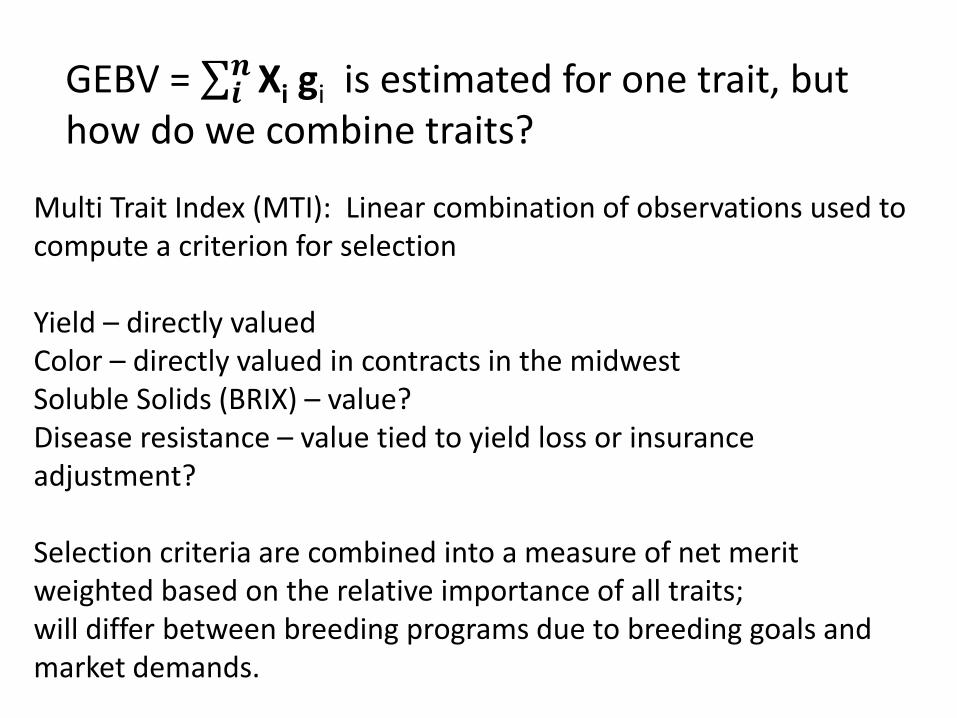
GEBV = Xi gi𝒏𝒊 is estimated for one trait, but
how do we combine traits?
Multi Trait Index (MTI): Linear combination of observations used to compute a criterion for selection Yield – directly valued Color – directly valued in contracts in the midwest Soluble Solids (BRIX) – value? Disease resistance – value tied to yield loss or insurance adjustment? Selection criteria are combined into a measure of net merit weighted based on the relative importance of all traits; will differ between breeding programs due to breeding goals and market demands.
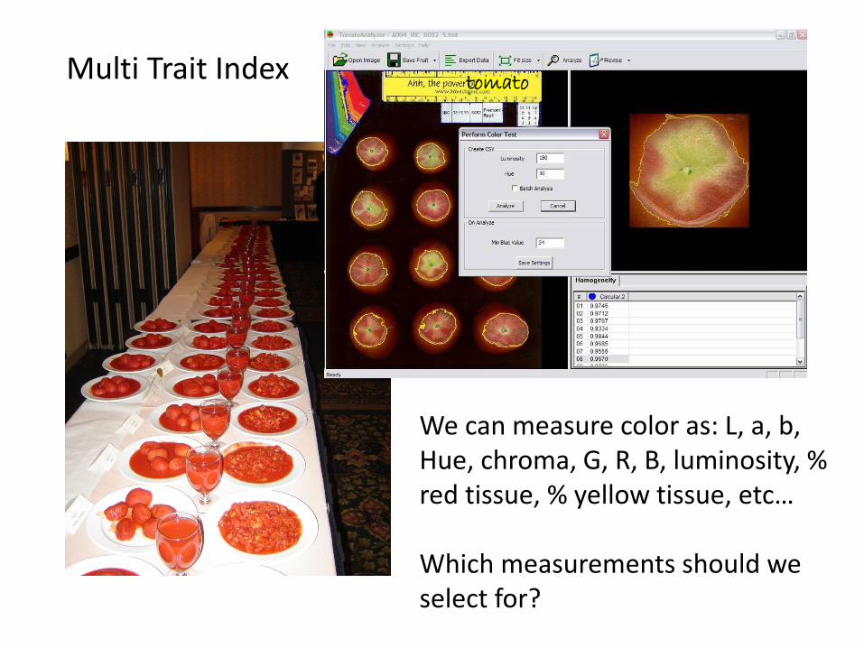
Multi Trait Index tomato
We can measure color as: L, a, b, Hue, chroma, G, R, B, luminosity, % red tissue, % yellow tissue, etc… Which measurements should we select for?
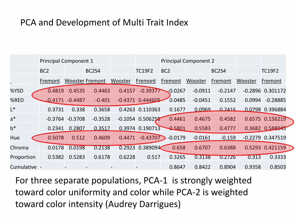
PCA and Development of Multi Trait Index
Principal Component 1 Principal Component 2
BC2 BC2S4 TC19F2 BC2 BC2S4 TC19F2
Fremont Wooster Fremont Wooster Fremont Fremont Wooster Fremont Wooster Fremont
%YSD 0.4819 0.4535 0.4463 0.4157 -0.39377 -0.0267 -0.0911 -0.2147 -0.2896 0.301172
%RED -0.4171 -0.4487 -0.401 -0.4371 0.444605 0.0485 -0.0451 0.1552 0.0994 -0.28885
L* 0.3731 0.338 0.3658 0.4263 0.110363 0.1677 0.0969 0.2416 0.0798 0.396884
a* -0.3764 -0.3708 -0.3528 -0.1054 0.506258 0.4461 0.4675 0.4582 0.6575 0.156219
b* 0.2341 0.2807 0.3517 0.3974 0.190713 0.5801 0.5583 0.4777 0.3682 0.588045
Hue 0.5078 0.512 0.4609 0.4471 -0.43707 -0.0179 -0.0161 -0.159 -0.2279 0.347519
Chroma 0.0178 0.0198 0.2138 0.2923 0.389094 0.658 0.6707 0.6388 0.5293 0.421159
Proportion 0.5382 0.5283 0.6178 0.6228 0.517 0.3265 0.3138 0.2726 0.313 0.3333
Cumulative - - - - - 0.8647 0.8422 0.8904 0.9358 0.8503
For three separate populations, PCA-1 is strongly weighted toward color uniformity and color while PCA-2 is weighted toward color intensity (Audrey Darrigues)

Predicted Gen. Value relative to BLUP of Phenotype (BLR package)
http://genomics.cimmyt.org/
GEBV = Xi gi𝒏𝒊
Marker Value 0 -0.32 1 1.23 0 0.40 1 -0.75 1 0.86 Sum 1.42
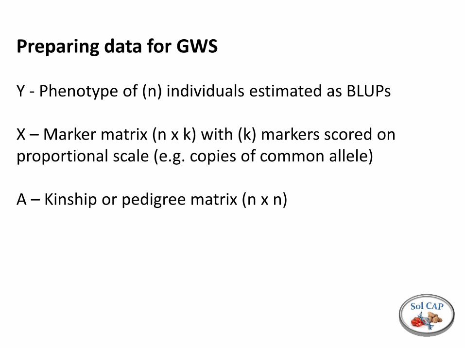
Preparing data for GWS Y - Phenotype of (n) individuals estimated as BLUPs X – Marker matrix (n x k) with (k) markers scored on proportional scale (e.g. copies of common allele) A – Kinship or pedigree matrix (n x n)
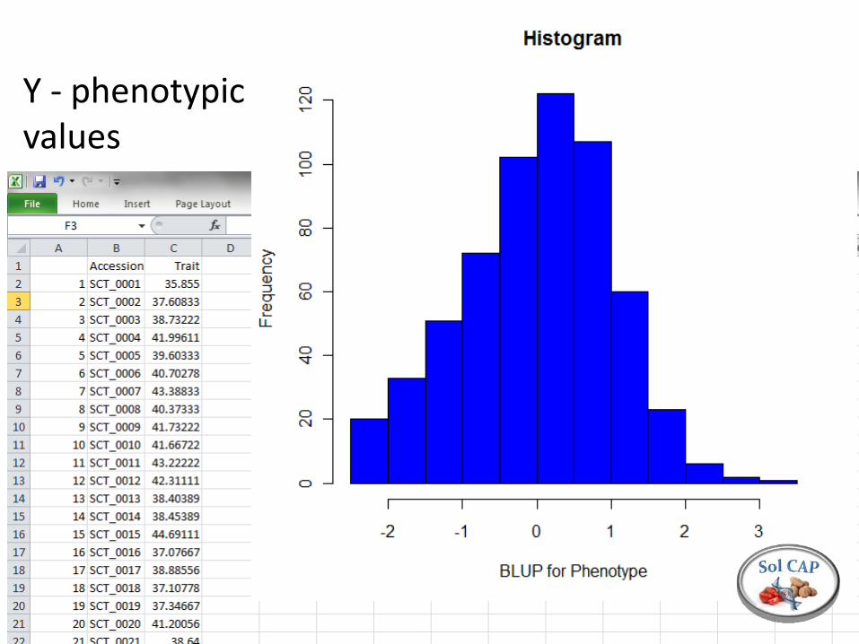
Y - phenotypic values
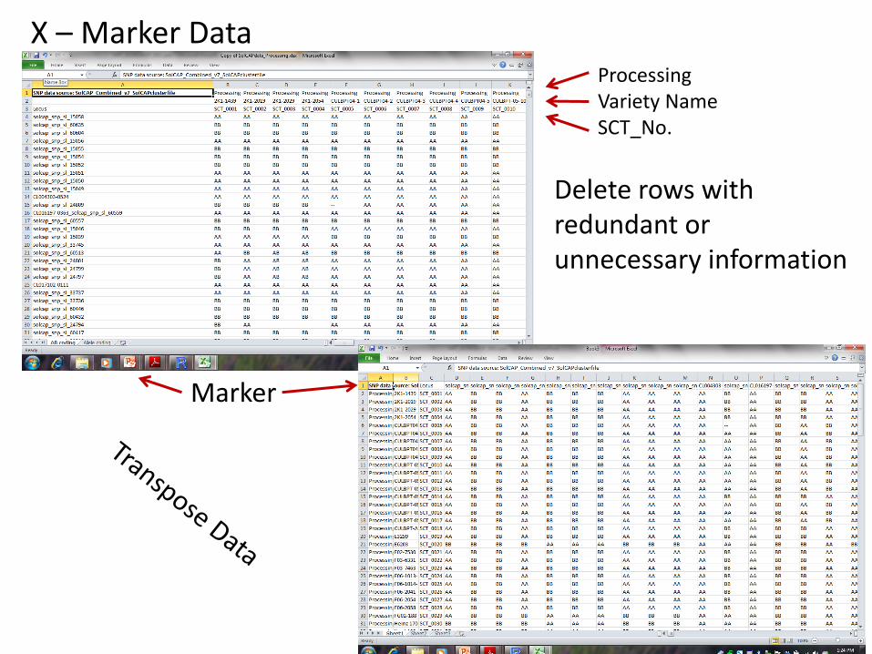
Processing Variety Name SCT_No.
Marker
Delete rows with redundant or unnecessary information
X – Marker Data
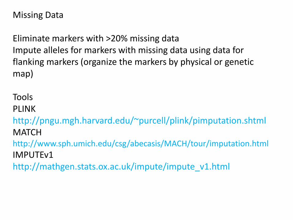
Missing Data Eliminate markers with >20% missing data Impute alleles for markers with missing data using data for flanking markers (organize the markers by physical or genetic map) Tools PLINK http://pngu.mgh.harvard.edu/~purcell/plink/pimputation.shtml MATCH http://www.sph.umich.edu/csg/abecasis/MACH/tour/imputation.html
IMPUTEv1 http://mathgen.stats.ox.ac.uk/impute/impute_v1.html
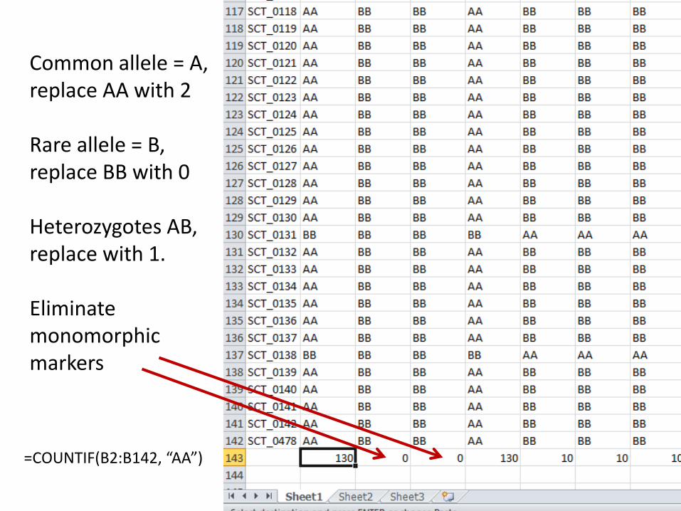
Common allele = A, replace AA with 2 Rare allele = B, replace BB with 0 Heterozygotes AB, replace with 1. Eliminate monomorphic markers
=COUNTIF(B2:B142, “AA”)
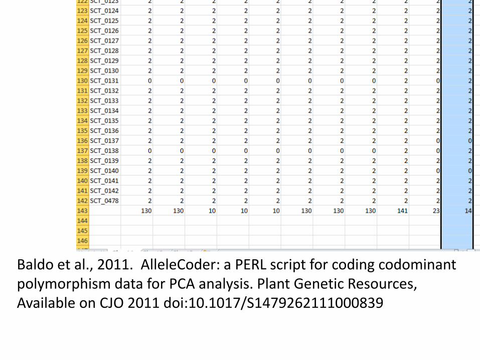
Baldo et al., 2011. AlleleCoder: a PERL script for coding codominant polymorphism data for PCA analysis. Plant Genetic Resources, Available on CJO 2011 doi:10.1017/S1479262111000839

Data Phenotype matrix (Y) Marker matrix (X) Kinship Matrix (A) MSA http://i122server.vu-wien.ac.at/MSA/MSA_download.html
See tutorials: http://www.extension.org/pages/32370/
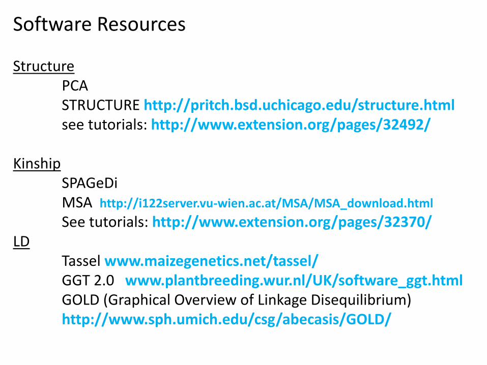
Software Resources Structure PCA STRUCTURE http://pritch.bsd.uchicago.edu/structure.html see tutorials: http://www.extension.org/pages/32492/ Kinship SPAGeDi MSA http://i122server.vu-wien.ac.at/MSA/MSA_download.html
See tutorials: http://www.extension.org/pages/32370/ LD Tassel www.maizegenetics.net/tassel/ GGT 2.0 www.plantbreeding.wur.nl/UK/software_ggt.html GOLD (Graphical Overview of Linkage Disequilibrium) http://www.sph.umich.edu/csg/abecasis/GOLD/
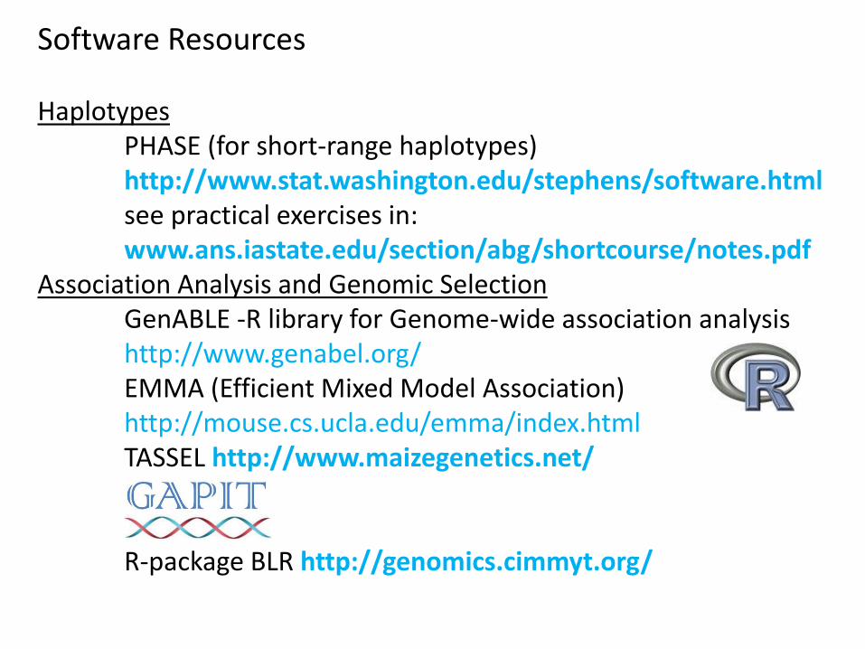
Software Resources Haplotypes PHASE (for short-range haplotypes) http://www.stat.washington.edu/stephens/software.html see practical exercises in: www.ans.iastate.edu/section/abg/shortcourse/notes.pdf Association Analysis and Genomic Selection GenABLE -R library for Genome-wide association analysis http://www.genabel.org/ EMMA (Efficient Mixed Model Association) http://mouse.cs.ucla.edu/emma/index.html TASSEL http://www.maizegenetics.net/ R-package BLR http://genomics.cimmyt.org/
Working Examples

Power of association Studies R-package ldDesign http://cran.r-project.org/web/packages/ldDesign/ ldDesign documentation http://cran.r-project.org/web/packages/ldDesign/ldDesign.pdf
See example script under “Practical Exercises”; Hayes, 2007. QTL Mapping, MAS, and Genomic Selection, Short Course Sponsored by Dept. of Animal Sciences and Animal Breeding and Genetics Group, Iowa State University http://www.ans.iastate.edu/section/abg/shortcourse/notes.pdf Other functions: ld.design , ld.power, ld.sim, etc...
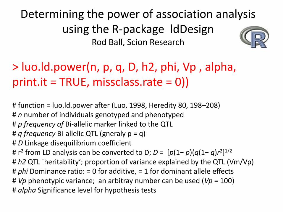
Determining the power of association analysis using the R-package ldDesign
Rod Ball, Scion Research
> luo.ld.power(n, p, q, D, h2, phi, Vp , alpha, print.it = TRUE, missclass.rate = 0)) # function = luo.ld.power after (Luo, 1998, Heredity 80, 198–208) # n number of individuals genotyped and phenotyped # p frequency of Bi-allelic marker linked to the QTL # q frequency Bi-allelic QTL (gneraly p = q) # D Linkage disequilibrium coefficient # r2 from LD analysis can be converted to D; D = [p(1− p)(q(1− q)r2]1/2
# h2 QTL `heritability‘; proportion of variance explained by the QTL (Vm/Vp) # phi Dominance ratio: = 0 for additive, = 1 for dominant allele effects # Vp phenotypic variance; an arbitray number can be used (Vp = 100) # alpha Significance level for hypothesis tests
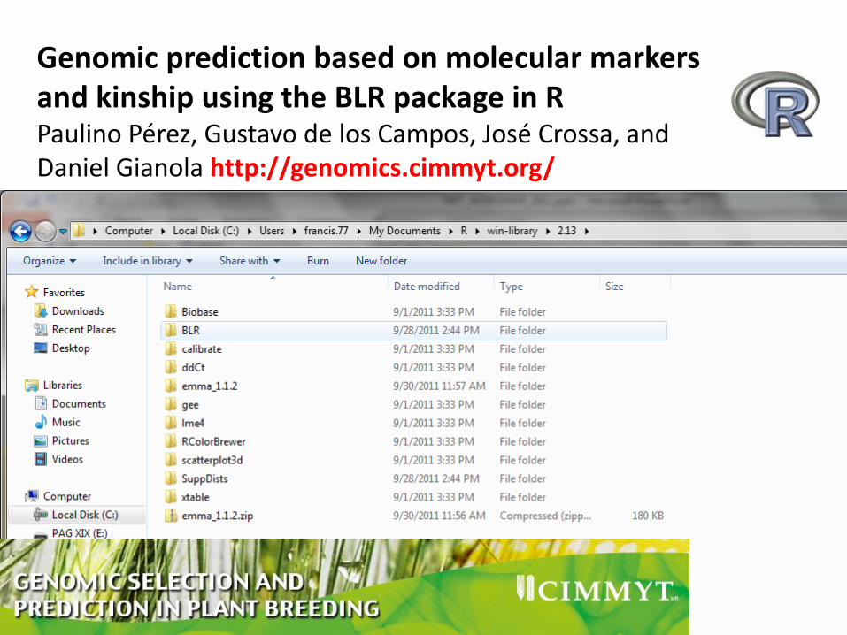
Genomic prediction based on molecular markers and kinship using the BLR package in R Paulino Pérez, Gustavo de los Campos, José Crossa, and Daniel Gianola http://genomics.cimmyt.org/
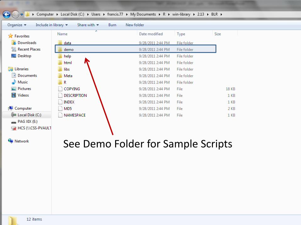
See Demo Folder for Sample Scripts
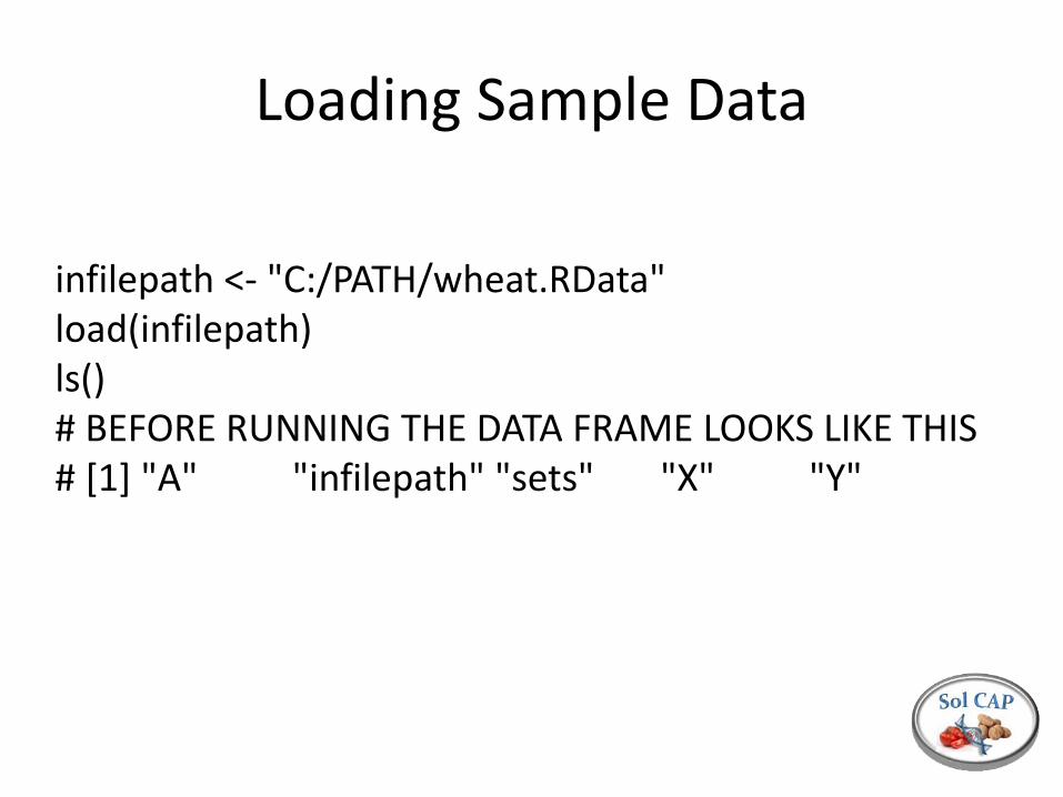
Loading Sample Data
infilepath <- "C:/PATH/wheat.RData" load(infilepath) ls() # BEFORE RUNNING THE DATA FRAME LOOKS LIKE THIS # [1] "A" "infilepath" "sets" "X" "Y"
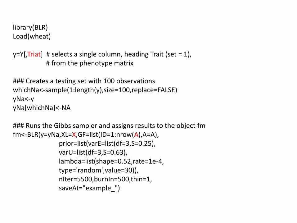
library(BLR) Load(wheat) y=Y[,Triat] # selects a single column, heading Trait (set = 1), # from the phenotype matrix ### Creates a testing set with 100 observations whichNa<-sample(1:length(y),size=100,replace=FALSE) yNa<-y yNa[whichNa]<-NA ### Runs the Gibbs sampler and assigns results to the object fm fm<-BLR(y=yNa,XL=X,GF=list(ID=1:nrow(A),A=A), prior=list(varE=list(df=3,S=0.25), varU=list(df=3,S=0.63), lambda=list(shape=0.52,rate=1e-4, type='random',value=30)), nIter=5500,burnIn=500,thin=1, saveAt="example_")
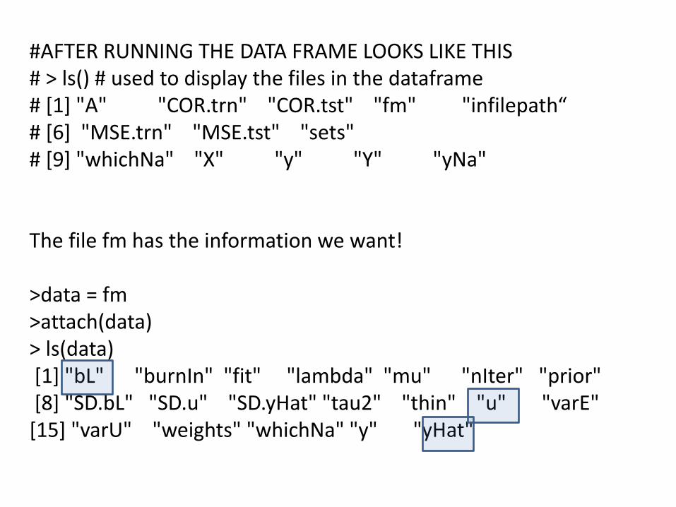
#AFTER RUNNING THE DATA FRAME LOOKS LIKE THIS # > ls() # used to display the files in the dataframe # [1] "A" "COR.trn" "COR.tst" "fm" "infilepath“ # [6] "MSE.trn" "MSE.tst" "sets" # [9] "whichNa" "X" "y" "Y" "yNa" The file fm has the information we want! >data = fm >attach(data) > ls(data) [1] "bL" "burnIn" "fit" "lambda" "mu" "nIter" "prior" [8] "SD.bL" "SD.u" "SD.yHat" "tau2" "thin" "u" "varE" [15] "varU" "weights" "whichNa" "y" "yHat"

Writing output to files > data2 = bL > write.csv(data2, "C:/PATH/data2.csv") > data3 = u > write.csv(data3, "C:/PATH/data3.csv") > data4 = yHat > write.csv(data4, "C:/PATH/data4.csv")
Concluding remarks: Accurate and objective phenotypes remain a limiting factor for tomato Most of the changes in breeding strategy that will improve the power/efficiency of GWS will also improve traditional phenotype-based breeding Use BLUPs to estimate trait values Use pedigree/kinship information to strengthen estimates of breeding values of individuals based on trait BLUPs Use larger populations
Acknowledgments
Collaborators, OSU
Heather Merk
Sung-Chur Sim
Troy Aldrich
Matt Robbins
Audrey Darrigues
Industry
Collaborators Cindy Lawley
Martin Ganal
Collaborators, UIB Hipolito Medrano
Pep Cifre
Josefina Bota
Miquel Angel Conesa
Funding USDA/AFRI
This project is supported by the Agriculture and Food
Research Initiative of USDA’s National Institute of Food and
Agriculture.
Collaborators, MSU
David Douches
C Robin Buell
John Hamilton
Kelly Zarka
Collaborators, Cornell
Walter de Jong
Lucas Mueller
Joyce van Eck
Naama Menda
Collaborators, UCD
Allen Van Deynze
Kevin Stoffel
Alex Kozic
Center
PBG Webinar Series • Putting research into practice • Suggest topics • Sign up to present
Contact: Heather Merk [email protected]