Embed Size (px)
Citation preview
Geodesics in geometry with constraints and
applications
I. Markina
REPORT No. 8, 2011/2012, fall
ISSN 1103-467XISRN IML-R- -8-11/12- -SE+fall
GEODESICS IN GEOMETRY WITH CONSTRAINTS ANDAPPLICATIONS
IRINA MARKINA
Lectures in Summer School
Analysis - with Applications to Mathematical Physics
GottingenGeorg - August-Universitat
August 29 - September 2, 2011
1
2 IRINA MARKINA
Abstract. In this course we will carefully define the notion of a non-holonomic man-ifold wich is a manifold with a certain non-integrable distribution. We will definesuch concepts as horizontal distribution, the Ehresmann connection, bracket generat-ing condition for a distribution, sub-Riemannian structure and sub-Riemannian metric,Hamiltonian system, normal and abnormal geodesics, principal bundle and others. Thelectures will be organized as follows.
Lecture 1. Notion of sub-Riemannian geometry and comparison with Riemannian geometry.Lecture 2. From the Heisenberg group to Carnot groups.Lecture 3. Principle bundles and Hopf maps for spheres. Geodesics on principle bundles.Lecture 4. Kaluza-Klein model and sub-Riemannian geometry.Lecture 5. Rolling of manifolds without slipping and twisting.Lecture 6. Group of diffeomorphisms of the unit circle as a principal U(1)-bundle.
Contents
1. Introduction 32. Main definitions 42.1. Smooth manifolds, vector fields, tangent map 42.2. Distributions and non-holonomic constraints 72.3. Riemannian and sub-Riemannian manifolds 112.4. Hamiltonian formalism and geodesics 123. Carnot groups 183.1. Short introduction to Lie groups 183.2. Heisenberg group 213.3. H-type groups 303.4. Carnot groups 414. Sub-Riemannian spheres 434.1. Sub-Riemannian structures on S3 434.2. Sub-Riemannian structures on S7 495. Principal bundles 545.1. Ehresmann connection 545.2. Metrics on principal bundles 555.3. Geodesics theorem 585.4. Geodesics related to Yang-Mills fields. 655.5. Examples of solutions to the Wong equations 756. Rolling manifolds 786.1. Extrinsic rolling 796.2. Intrinsic rolling 816.3. Distributions for extrinsic and intrinsic rolling 886.4. Examples of rollings and their controllability 917. Group of diffeomorphisms of the circle 977.1. Manifold and group structure of Diff S1. 977.2. Sub-Riemannian geodesics on Diff S1. 1138. Appendix A 1198.1. Smooth manifolds 1198.2. Symplectic manifolds 122
GEOMETRY WITH CONSTRAINTS 3
8.3. Lie groups 1238.4. Complexifications 1328.5. Fiber bundles 1359. Appendix B 137References 141
1. Introduction
These notes are based on the course of lectures presented at the summer school “Anal-ysis - with Applications to Mathematical Physics” that took place at Gottingen Georg -August - Universitat, Gottingen, in August 29 - September 2, 2011. The main purposeof these notes is to give a flavor of the subject that during last decade received the nameSub - Riemannian Geometry and that studies the geometry of manifolds with non -holonomic constraints. This subject has attracted attention of scientists since 19-s cen-tury. We will not describe the history of development of this subject, we only mentionthat it was independently considered in several branches of mathematics such as non -holonomic mechanics, geometry of bundles, CR manifolds, geometric control theory andothers.
It is supposed that the reader is familiar with basic notions of differential geometry,topology, and Lie groups. Nevertheless, in order to keep self - sufficiency of the notes,we present main definitions and basic notions related to these topics in the Appendix A.It is advisable to consult first the Appendix A, if the reader meets an unfamiliar notion.
The principal subject of the sub - Riemannain geometry, discussed in the notes, isgeodesics related to sub - Riemannian Hamiltonian functions produced by a sub - Rie-mannian metric. We present basic models where the sub-Riemannian geometry appearsrather naturally. Based on these examples we show main features and peculiarities ofgeodesics in geometry with non-holonomic constraints. The structure of notes is as fol-lows. Section 2 collects main definitions that reveal the similarity and difference betweenRiemannian and sub - Riemannian geometries. Carnot groups and their particular ex-amples are presented in Section 3. We describe the sub-Riemannian structure of odddimensional spheres in Section 4. Section 5 deals with principal bundles. After pre-senting main definitions we reconsider examples of Sections 3 and 4 from the point ofview of principal bundles. Sections 6 is dedicated to a mechanical problem of rollingone manifold over another, where kinematic constraints described in the language of asmooth sub - bundle of the tangent bundle of the configuration space. In the last Section7 we generalize some results obtained for principal bundles on the infinite dimensionalLie group of orientation preserving diffeomorphisms of the unit circle. Appendix A col-lects avast of definitions and concrete formulas used in the text. Some of them are wellknown, some of them are not widely presented in the literature. As it was noticed above,we recommend for a not very experienced reader to start reading the notes from Appen-dix A. Appendix B is short and very technical, where we wrote some of the expressionsthat are useful, but not necessary for the first reading.
4 IRINA MARKINA
1.0.1. Acknowledgments. It is not a duty, but a pleasure to thank the organizers of theschool “Analysis - with Applications to Mathematical Physics” in Gottingen, and inparticular, Wolfram Bauer, for the invitation, warm hospitality and an extraordinarilyinteresting school.
I am grateful to the Analysis Group at the University of Bergen for the creative friendlyatmosphere and the infinite source of ideas, questions and emotions. Particularly, I wouldlike to express deep gratitude to my co-authors with whom I shared hard hours of workand lovely time of mathematical conversations.
Special sincere thanks to my lovely husband Alexander Vasiliev for his support of allmy initiatives.
I also appreciate the warm hospitality of the research program ”Complex Analysis andIntegrable Systems” held at the Mittag-Leffler Institute, Stockholm, Sweden, during thefall 2012, where these notes were finished. Finally, my thanks go to Norwegian ResearchCouncil supported me by the project # 204726 /V30.
2. Main definitions
2.1. Smooth manifolds, vector fields, tangent map. It is supposed that the readeris familiar with the notion of smooth or C∞ manifolds. We set up main definitions andnotations. A smooth manifold is a Hausdorff, second countable topological space, wherethe smooth complete atlas is defined. We write M for a smooth manifold, or rather Mn
if we want to emphasize the dimension n of the manifold. Let C∞(M) denote the spaceof smooth real valued functions defined on M .
The tangent space at a point q ∈ M is denoted by TqM . Remind that any elementvq ∈ TqM is a function vq : C∞(M) → R satisfying two properties
1. R-linearity: vq(af + bg) = avq(f) + bvq(g),2. Leibnizian property: vq(fg) = vq(f)g(q) + f(q)vq(g)
for all a, b ∈ R, f, g ∈ C∞(M), q ∈ M . The space TqM , q ∈ M , is a real vector spaceand therefore vq is called tangent vector.
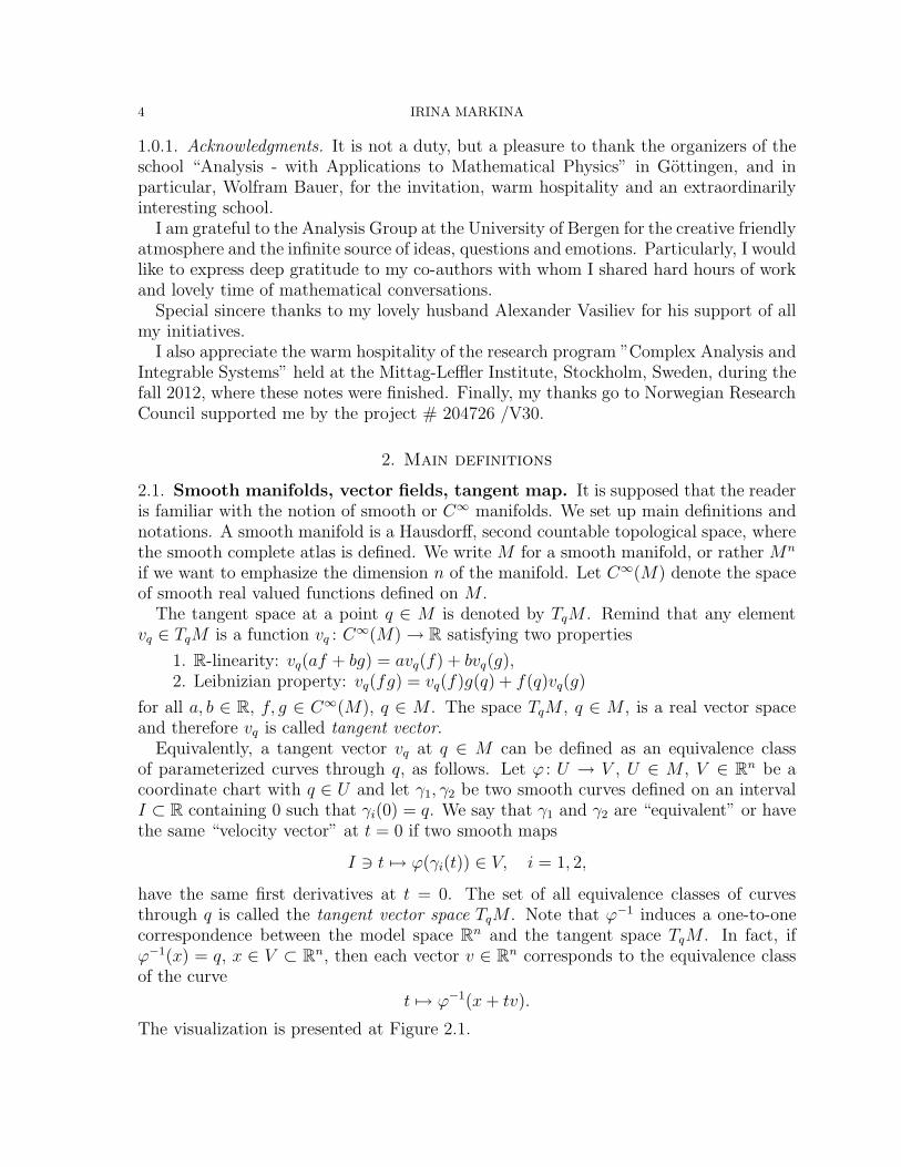
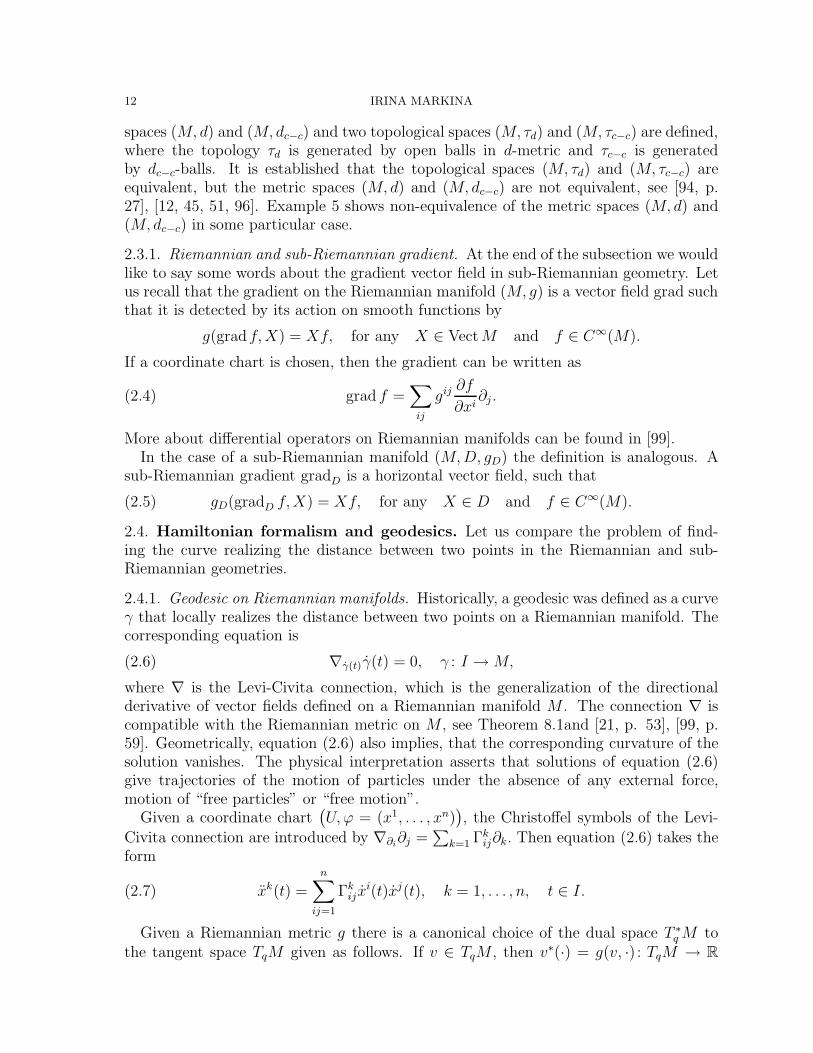
Equivalently, a tangent vector vq at q ∈ M can be defined as an equivalence classof parameterized curves through q, as follows. Let ϕ : U → V , U ∈ M , V ∈ Rn be acoordinate chart with q ∈ U and let γ1, γ2 be two smooth curves defined on an intervalI ⊂ R containing 0 such that γi(0) = q. We say that γ1 and γ2 are “equivalent” or havethe same “velocity vector” at t = 0 if two smooth maps
I $ t %→ ϕ(γi(t)) ∈ V, i = 1, 2,
have the same first derivatives at t = 0. The set of all equivalence classes of curvesthrough q is called the tangent vector space TqM . Note that ϕ−1 induces a one-to-onecorrespondence between the model space Rn and the tangent space TqM . In fact, ifϕ−1(x) = q, x ∈ V ⊂ Rn, then each vector v ∈ Rn corresponds to the equivalence classof the curve
t %→ ϕ−1(x + tv).
The visualization is presented at Figure 2.1.
GEOMETRY WITH CONSTRAINTS 5
pU
x
I
R
0
Rn
M
γ1
γ2ϕϕ−1
Vα ϕ γ1
ϕ γ2v
0
Figure 2.1. The notion of the tangent vector
After previous definitions one can also say, that the notion of a tangent vector vis the generalization of the derivative of C∞-functions along the direction v. If thechart
(U,ϕ = (x1, . . . , xn)
)is chosen, then the standard notation for the basis of TqM is(
∂∂x1 , . . . ,
∂∂xn
)or shortly (∂1, . . . , ∂n). Any vector v ∈ TqM will be written in coordinates
as v =∑n
j=1 vj∂j . Notice the position of indices!
The dual space to TqM is denoted by T ∗q M and the pairing is written as 〈·, ·〉q, wherewe usually omit the subscript “q”, see Definition 42. The dual basis to (∂1, . . . , ∂n) withrespect to the pairing is denoted by (dx1, . . . , dxn). Then any co-vector λ ∈ T ∗q M is
written in coordinates as λ =∑n
k=1 λkdxk. Notice the position of indices. So we have〈dxi, ∂j〉 = δij , where δij is the Kronecker symbol. The elements of T ∗M are usuallycalled co-vectors in geometry and momenta in physics.
The tangent and co-tangent bundles are denoted by TM and T ∗M , correspondingly,consult Definition 58. Both vector bundles are C∞-smooth manifolds [21, 99]. Thenotations
prM : TM → M and pr∗M : T ∗M → M(q, v) → q (q,λ) → q
will be fixed for canonical projections from the tangent and co-tangent bundles to theunderlying manifold.
A vector field X on a manifold M is a function that assigns to each point q ∈ M atangent vector X(q) ∈ TqM . We also write Xq for the value of the vector field X atpoint q ∈ M . If f ∈ C∞(M), then Xf denotes a real valued function on M given by
(Xf)(q) = X(q)f, for all q ∈ M.
6 IRINA MARKINA
ψ(V )
ϕ(U)
ψ F ϕ−1
ψ
ϕ
M
N
F
U
V
qF (q)
Figure 2.2. The smooth map F
A vector field X is called smooth if for any f ∈ C∞(M) the function Xf : M → R isalso from C∞(M). If
(U,ϕ = (x1, . . . , xn)
)is a coordinate chart, then any vector field X
can be written in terms of coordinates as X(q) =∑n
j=1 Xj(q)∂j. Then the smoothnesscondition of the vector field X on the neighborhood U is equivalent to the requirementthat all functions Xj, j = 1, . . . , n, are of class C∞(U). If the functions Xj , j = 1, . . . , n,are analytic in U , then the corresponding vector field X is called an analytic vector field.
Another way to define a vector field X is to use the definition of a local section.Namely, a vector fields X is a smooth map X : M → TM , such that prM X = idU forany open set U ⊂ M . The section is global if U can be taken as entire M . We writeVect M (Vect U) for the collection of smooth vector fields, defined on M (U , U ⊂ M).Algebraically, Vect M is a module over the ring C∞(M) and a vector space over the fieldR (C). Moreover, the operation of multiplication of two vector fields is defined. Themultiplication [·, ·] (that received the name of commutator or the Lie product) is definedby
(2.1) [X, Y ]f = X(Y f)− Y (Xf).
The Lie product is a map [·, ·] : Vect M × Vect M → Vect M satisfying three axioms ofDefinition 50. The set of smooth vector fields considered as a real vector space endowedwith the Lie multiplication forms a Lie algebra.
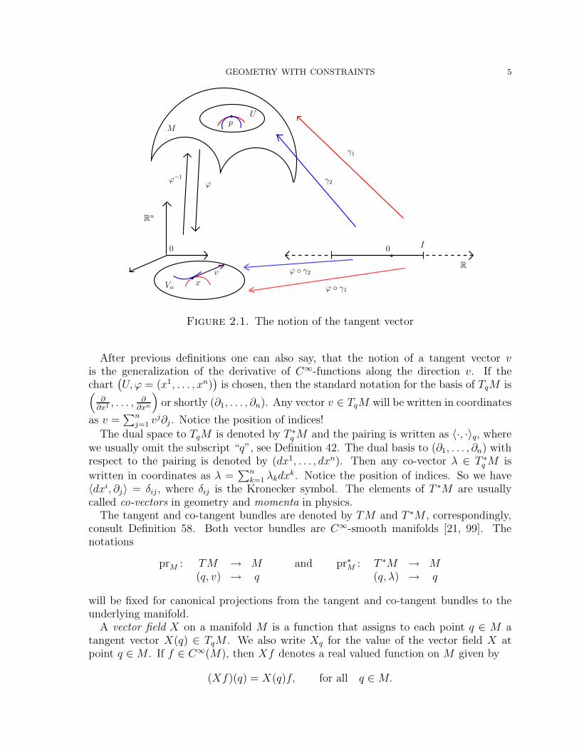
Definition 1. Let M and N be two smooth manifolds and F : M → N be a map. Themap F is smooth if the following holds. For any q ∈ M and for any local charts (U,ϕ)of q ∈ M and (V,ψ) of F (q) ∈ N , the composition ψ F ϕ−1 is a smooth map
ψ F ϕ−1 : ϕ(U) → ψ(V )
in the sense of smoothness defined in the Euclidean space.
The definition is illustrated in Figure 2.2. A diffeomorphism between two manifoldsis defined in a similar way.
GEOMETRY WITH CONSTRAINTS 7
Definition 2. Let F : M → N be a smooth map. The differential of F at q ∈ M is thelinear map dqF : TqM → TF (q)N .
If the local charts(U,ϕ = (x1, . . . , xm)
)of q ∈ M and
(V,ψ = (y1, . . . , yn)
)of
F (q) ∈ N are chosen, then
dqF (∂xj) =n∑
k=1
∂
∂xj
(yk
(F (q)
))∂yk |F (q), j = 1, . . . , m.
The matrix
∂∂xj
(yk
(F (q)
))k,j
is called the Jacobi matrix of the map F with respect
to the given coordinate charts.
2.2. Distributions and non-holonomic constraints.
Definition 3. Let M be a smooth manifold. A mapping D that assigns to every pointq ∈ M a linear subspace Dq of the tangent space TqM is called a singular distributionon M .
Definition 4. A distribution D is called smooth on M , if for any q ∈ M there is aneighborhood U(q) and smooth linearly independent vector fields X1, . . . , Xk, such thatDx = spanX1(x), . . . , Xk(x), for all x ∈ U(q).
A distribution D is called analytic if the vector fields X1, . . . , Xk in Definition 4 can bechosen to be analytic. The smooth (analytic) distribution D on M is a smooth (analytic)sub-bundle of the tangent bundle TM , and its rank is equal to k for all q ∈ M . In thecase of singular distribution the set of vector fields X1, . . . , Xk may not be necessarilylinear independent, and therefore, the dimension of the linear subspace Dq can vary frompoint to point.
From now on, we will work only with smooth distributions and smooth manifolds andtherefore we omit the word “smooth”. Analogous definition can be given for a map D∗
that assigns for any point q ∈ M a linear subspace in the co-tangent space T ∗q M and inthis case it is called a co-distribution.
The notion of a smooth distribution naturally leads to the following question. Whendoes a smooth distribution or a smooth sub-bundle D ⊂ TM define a submanifold Ninside of the original manifold M? The answer was given by Frobenius [38].
Definition 5. A smooth distribution D on M is called involutive or integrable if [X, Y ] ∈D for any choice of X and Y ∈ D.
Definition 6. A smooth submanifold N of a manifold M is the integral manifold of adistribution D if for any point q ∈ N there is an open neighborhood U(q) ⊂ N such thatTxN = Dx for any x ∈ U(q).
Theorem 2.1. [38, 113] A submanifold N of a manifold M is the integral manifold ofa distribution D, if and only if, D is involutive.
In this case a foliation of the manifold M by integral manifolds N passing throughdifferent points q ∈ M is produced. Somehow, one can not leave a chosen leaf of thefoliation being touched to the distribution.
8 IRINA MARKINA
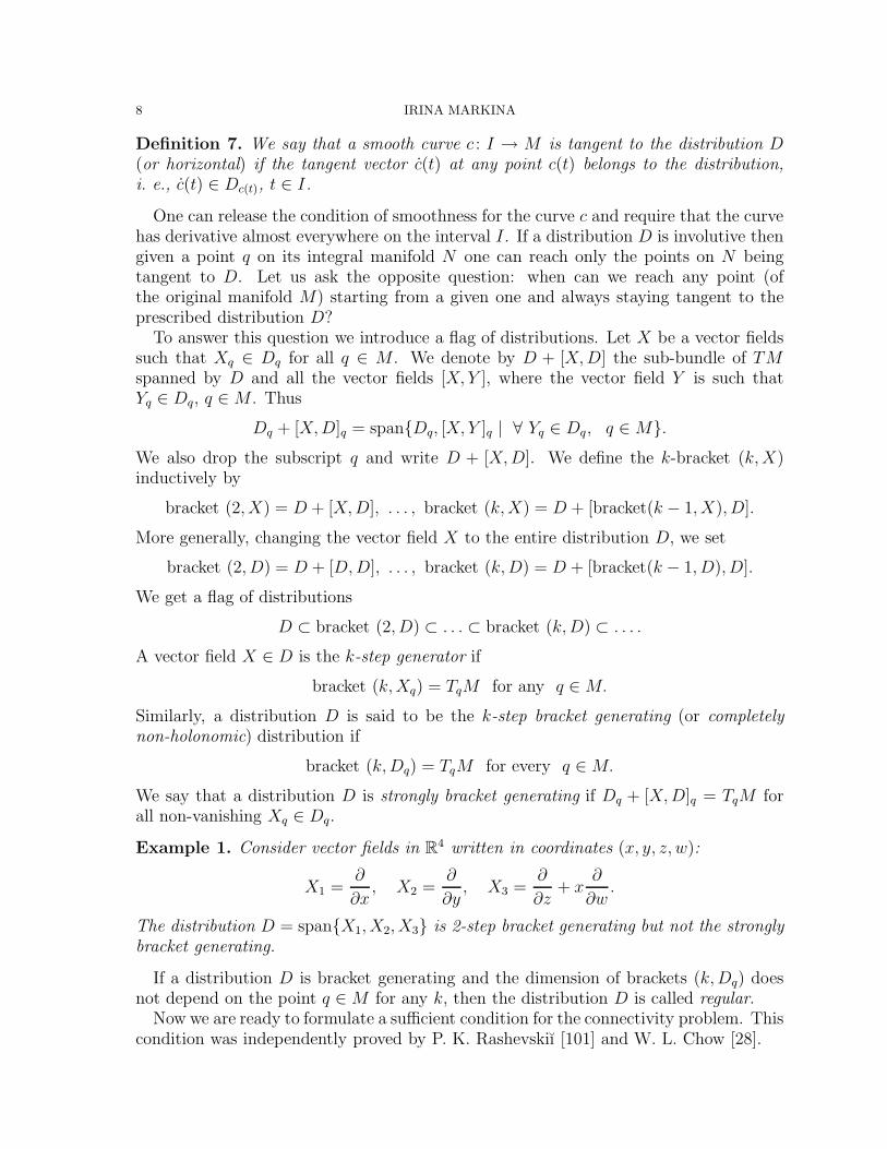
Definition 7. We say that a smooth curve c : I → M is tangent to the distribution D(or horizontal) if the tangent vector c(t) at any point c(t) belongs to the distribution,i. e., c(t) ∈ Dc(t), t ∈ I.
One can release the condition of smoothness for the curve c and require that the curvehas derivative almost everywhere on the interval I. If a distribution D is involutive thengiven a point q on its integral manifold N one can reach only the points on N beingtangent to D. Let us ask the opposite question: when can we reach any point (ofthe original manifold M) starting from a given one and always staying tangent to theprescribed distribution D?
To answer this question we introduce a flag of distributions. Let X be a vector fieldssuch that Xq ∈ Dq for all q ∈ M . We denote by D + [X, D] the sub-bundle of TMspanned by D and all the vector fields [X, Y ], where the vector field Y is such thatYq ∈ Dq, q ∈ M . Thus
Dq + [X, D]q = spanDq, [X, Y ]q | ∀ Yq ∈ Dq, q ∈ M.We also drop the subscript q and write D + [X, D]. We define the k-bracket (k, X)inductively by
bracket (2, X) = D + [X, D], . . . , bracket (k, X) = D + [bracket(k − 1, X), D].
More generally, changing the vector field X to the entire distribution D, we set
bracket (2, D) = D + [D, D], . . . , bracket (k, D) = D + [bracket(k − 1, D), D].
We get a flag of distributions
D ⊂ bracket (2, D) ⊂ . . . ⊂ bracket (k, D) ⊂ . . . .
A vector field X ∈ D is the k-step generator if
bracket (k, Xq) = TqM for any q ∈ M.
Similarly, a distribution D is said to be the k-step bracket generating (or completelynon-holonomic) distribution if
bracket (k, Dq) = TqM for every q ∈ M.
We say that a distribution D is strongly bracket generating if Dq + [X, D]q = TqM forall non-vanishing Xq ∈ Dq.
Example 1. Consider vector fields in R4 written in coordinates (x, y, z, w):
X1 =∂
∂x, X2 =
∂
∂y, X3 =
∂
∂z+ x
∂
∂w.
The distribution D = spanX1, X2, X3 is 2-step bracket generating but not the stronglybracket generating.
If a distribution D is bracket generating and the dimension of brackets (k, Dq) doesnot depend on the point q ∈ M for any k, then the distribution D is called regular.
Now we are ready to formulate a sufficient condition for the connectivity problem. Thiscondition was independently proved by P. K. Rashevskiı [101] and W. L. Chow [28].
GEOMETRY WITH CONSTRAINTS 9
y
x0
A
B
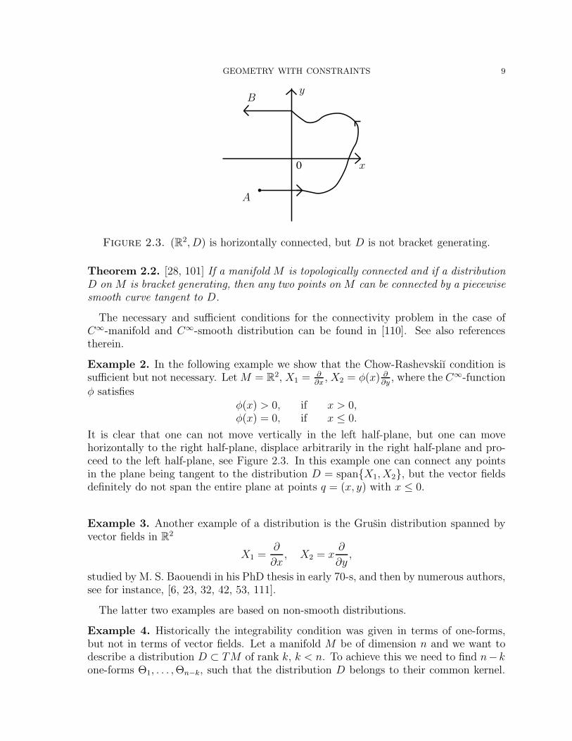
Figure 2.3. (R2, D) is horizontally connected, but D is not bracket generating.
Theorem 2.2. [28, 101] If a manifold M is topologically connected and if a distributionD on M is bracket generating, then any two points on M can be connected by a piecewisesmooth curve tangent to D.
The necessary and sufficient conditions for the connectivity problem in the case ofC∞-manifold and C∞-smooth distribution can be found in [110]. See also referencestherein.
Example 2. In the following example we show that the Chow-Rashevskiı condition issufficient but not necessary. Let M = R2, X1 = ∂
∂x, X2 = φ(x) ∂
∂y, where the C∞-function
φ satisfiesφ(x) > 0, if x > 0,φ(x) = 0, if x ≤ 0.
It is clear that one can not move vertically in the left half-plane, but one can movehorizontally to the right half-plane, displace arbitrarily in the right half-plane and pro-ceed to the left half-plane, see Figure 2.3. In this example one can connect any pointsin the plane being tangent to the distribution D = spanX1, X2, but the vector fieldsdefinitely do not span the entire plane at points q = (x, y) with x ≤ 0.
Example 3. Another example of a distribution is the Grusin distribution spanned byvector fields in R2
X1 =∂
∂x, X2 = x
∂
∂y,
studied by M. S. Baouendi in his PhD thesis in early 70-s, and then by numerous authors,see for instance, [6, 23, 32, 42, 53, 111].
The latter two examples are based on non-smooth distributions.
Example 4. Historically the integrability condition was given in terms of one-forms,but not in terms of vector fields. Let a manifold M be of dimension n and we want todescribe a distribution D ⊂ TM of rank k, k < n. To achieve this we need to find n− kone-forms Θ1, . . . ,Θn−k, such that the distribution D belongs to their common kernel.
10 IRINA MARKINA
The forms Θj, j = 1, . . . , n − k, are called annihilators. It is equivalent to solve thesystem
Θ1(x1, . . . , xn) = 0
. . . . . . . . . . . . . . .
Θn−k(x1, . . . , xn) = 0,
that received the name Pfaffian equations. This system is integrable if the one-formsΘ1, . . . ,Θn−k are exact forms:
(2.2)
Θ1(x
1, . . . , xn) = dθ1(x1, . . . , xn) = 0
. . . . . . . . . . . . . . .
Θn−k(x1, . . . , xn) = dθn−k(x
1, . . . , xn) = 0.
After integrating the latter system we get n − k functions describing a k-dimensionalintegral submanifold of M defined by integrable system (2.2) or by the involutive distri-bution D.
The Chow-Rashevskiı Theorem 2.2 for an analytic co-rank one distribution D, orfor one Pfaffian equation was solved by C. Caratheodory. The result states as follows.Let M be a connected manifold endowed with an analytic co-rank one distribution D. Ifthere exist two points A and B ∈ M that cannot be connected by a horizontal curve, thenthe distribution D is integrable. Or, formulating the negation of the above statement iffor any points A, B ∈ M there is a horizontal curve connecting these points, then thedistribution D is non-integrable (completely non-holonomic, bracket generating).
C. Caratheodory developed this theory due to the question posted by M. Born toderive the second law of thermodynamics and the existence of the entropy function.Translating the problem into the geometric language we work with a manifold M that isthe set of all possible thermodynamical states of some isolated system. The admissibleor horizontal curves are adiabatic curves, such curves that correspond to slow processesin time T and such that during these processes (along the admissible curves) no heat Θis exchanged. C. Caratheodory wrote the condition of an adiabatic process as a Pfaffianequation Θ = 0 on M . It was known at that moment from works by S. Carnot, J. P. Jouleand others, that there are thermodynamical states A, B ∈ M , which cannot be connectedby an adiabatic process (by an admissible curve). Caratheodory’s theorem states in thiscase that the distribution defined by the Pfaffian equation Θ = 0 is integrable, thatleads to the existence of two functions T (time) and S (entropy) that locally satisfythe relation Θ = TdS. This proves the existence of the entropy function S, as wellas that the adiabatic process remains in the leaf (hypersurface) of the state space Mcorresponding to the entropy function. The entropy function S tends not to decrease,being constant or increasing, according to the second law of thermodynamics.
Due to the names of S. Carnot and C. Caratheodory involved into this discovery,M. Gromov called the sub-Riemannian geometry as the Carnot-Caratheodory geometry.
Exercises.
Define whether the following distributions D = spanX1, X2 in R3 are bracket gen-erating and regular. Find one forms ω such that D = ker(ω).
1. Heisenberg distribution: X1 = ∂∂x
, X2 = ∂∂y
+ x ∂∂z
.
GEOMETRY WITH CONSTRAINTS 11
2. Martinet distribution: X1 = ∂∂x
, X2 = ∂∂y
+ x2 ∂∂z
.
2.3. Riemannian and sub-Riemannian manifolds. Let us recall some notions fromthe Riemannian geometry and compare basic definitions in the Riemannian and sub-Riemannian settings.
Definition 8. A Riemannian metric is a map g : TM ×TM → R, which is symmetric,bilinear, positively definite for any q ∈ M , and smoothly varying with respect to q ∈ M .
If the coordinate chart(U,ϕ = (x1, . . . , xn)
)is chosen and (∂1, . . . , ∂n) is the local
basis of TqM , q ∈ U , then gij = g(∂i, ∂j) is the associated matrix to the metric g.Smoothness of g means that the matrix gij(q) = gij(x
1, . . . , xn) is a smooth function of(x1, . . . , xn) in ϕ(U).
The couple (M, g) is called the Riemannian manifold. It would be more correct to saythat the triplet (M, TM, g) is called the Riemannian manifold.
Definition 9. The distance d(q0, q1) between two points q0, q1 ∈ M related to the Rie-mannian metric g is defined by the equality
d(q0, q1) = inf∫ 1
0
(g(c(t), c(t)
))1/2
dt,
where the infimum is taken over all curves c : [0, 1] → M differentiable almost everywhere in [0, 1], and such that c(0) = q0, c(1) = q1.
We are ready now to define a sub-Riemannian manifold. Let M be a smooth manifoldand let D be a smooth distribution (a smooth sub-bundle) of the tangent bundle TM .
Definition 10. A map gD : D×D → R which is symmetric, bilinear, positively definitefor any q ∈ M and smoothly varying with respect to q is called a sub-Riemannian metric.
Definition 11. The couple (D, gD) is called a sub-Riemannian structure and the triplet(M, D, gD) is called a sub-Riemannian manifold.
If D = TM , then Definition 11 is reduced to the definition of the Riemannian mani-fold. In this sense the sub-Riemannian geometry is a generalization of the Riemanniangeometry. The distance function related to the sub-Riemannian metric gD is defined by
(2.3) dc−c(q0, q1) = inf∫ 1
0
(gD
(c(t), c(t)
))1/2
dt
,
where the infimum is taken over all horizontal curves c : [0, 1]→M differentiable almostevery where in [0, 1] and such that c(0) = q0, c(1) = q1. Thus, we have added thehorizontality condition c(t) ∈ Dc(t) for the set of admissible curves. The set of admissiblecurves is smaller, therefore, dc−c-distance is, in general, bigger than the Riemanniandistance if both metrics are defined on the manifold. Theorem 2.2 guaranties thatthe set of horizontal curves is not empty and in this case the function dc−c takes onlyfinite values. The distance dc−c is called the Carnot-Caratheodory distance due to theadiabatic process studied by S. Carnot and the impact by C.Caratheodory described inExample 4. Let us suppose that a Riemannian metric g and a sub-Riemannian metricgD are defined on a smooth manifold M , and the Riemannian distance d and the Carnot-Caratheodory distance dc−c on M are produced, respectively. As a result, two metric
12 IRINA MARKINA
spaces (M, d) and (M, dc−c) and two topological spaces (M, τd) and (M, τc−c) are defined,where the topology τd is generated by open balls in d-metric and τc−c is generatedby dc−c-balls. It is established that the topological spaces (M, τd) and (M, τc−c) areequivalent, but the metric spaces (M, d) and (M, dc−c) are not equivalent, see [94, p.27], [12, 45, 51, 96]. Example 5 shows non-equivalence of the metric spaces (M, d) and(M, dc−c) in some particular case.
2.3.1. Riemannian and sub-Riemannian gradient. At the end of the subsection we wouldlike to say some words about the gradient vector field in sub-Riemannian geometry. Letus recall that the gradient on the Riemannian manifold (M, g) is a vector field grad suchthat it is detected by its action on smooth functions by
g(grad f, X) = Xf, for any X ∈ Vect M and f ∈ C∞(M).
If a coordinate chart is chosen, then the gradient can be written as
(2.4) grad f =∑ij
gij ∂f
∂xi∂j .
More about differential operators on Riemannian manifolds can be found in [99].In the case of a sub-Riemannian manifold (M, D, gD) the definition is analogous. A
sub-Riemannian gradient gradD is a horizontal vector field, such that
(2.5) gD(gradD f, X) = Xf, for any X ∈ D and f ∈ C∞(M).
2.4. Hamiltonian formalism and geodesics. Let us compare the problem of find-ing the curve realizing the distance between two points in the Riemannian and sub-Riemannian geometries.
2.4.1. Geodesic on Riemannian manifolds. Historically, a geodesic was defined as a curveγ that locally realizes the distance between two points on a Riemannian manifold. Thecorresponding equation is
(2.6) ∇γ(t)γ(t) = 0, γ : I →M,
where ∇ is the Levi-Civita connection, which is the generalization of the directionalderivative of vector fields defined on a Riemannian manifold M . The connection ∇ iscompatible with the Riemannian metric on M , see Theorem 8.1and [21, p. 53], [99, p.59]. Geometrically, equation (2.6) also implies, that the corresponding curvature of thesolution vanishes. The physical interpretation asserts that solutions of equation (2.6)give trajectories of the motion of particles under the absence of any external force,motion of “free particles” or “free motion”.
Given a coordinate chart(U,ϕ = (x1, . . . , xn)
), the Christoffel symbols of the Levi-
Civita connection are introduced by ∇∂i∂j =
∑k=1 Γ
kij∂k. Then equation (2.6) takes the
form
(2.7) xk(t) =
n∑ij=1
Γkij x
i(t)xj(t), k = 1, . . . , n, t ∈ I.
Given a Riemannian metric g there is a canonical choice of the dual space T ∗q M tothe tangent space TqM given as follows. If v ∈ TqM , then v∗(·) = g(v, ·) : TqM → R
GEOMETRY WITH CONSTRAINTS 13
is a linear functional, and therefore, the element of T ∗q M . In coordinates it gives thefollowing. Let ∂jn
j=1 be a basis of TqM and let gij be the matrix associated with the
metric g, then dxi =∑n
j=1 gij∂j , i = 1, . . . , n, represent the basis of the dual T ∗q M .
If v =∑n
j=1 vj∂j then v∗ =∑n
i=1 v∗i dxi, where v∗i =∑n
j=1 gijvj. This process is called
“lowering indices” in physics.We can say now that the Riemannian metric g defines a map g : TqM → T ∗q M , which
is an isomorphism between two vector spaces. Therefore, the inverse map g−1 : T ∗q M →TqM is defined. The map g−1 defines a metric on T ∗q M , called a co-metric, which we
denote by g−1. Thus, the co-metric is the map g−1 : T ∗q M × T ∗q M → R defined by
g−1(v∗, w∗) = v∗(g−1(w∗)
)= g
(g−1(v∗), g−1(w∗)
).
We see that maps g and g−1 became isometries. The matrix corresponding to g−1 is theinverse matrix to gij and it is usually written as gij. The process that associates avector v = (v1, . . . , vn) to a given co-vector λ = (λ1, . . . ,λn) by making use of the mapg−1 is called “rising indices”:
vi =n∑
j=1
gijλj, i = 1, . . . , n.
We conclude that the Riemannian metric g defines a pairing
〈·, ·〉 : T ∗q M × TqM → R
by
〈λ, v〉 = g(g−1(λ), v) = g−1(λ, g(v)), λ ∈ T ∗q M, v ∈ TqM.
Having the co-metric and chosen coordinate chart, we define the Riemannian Hamil-tonian function H : T ∗M → R by
H(q,λ) =1
2g−1(λq,λq) =
1
2
n∑i,j=1
gijλiλj .
A solution of the Hamiltonian equations
xi =∂H(q,λ)
∂λi, q = (x1, . . . , xn)(2.8)
λi = −∂H(q,λ)
∂xi, λ = (λ1, . . . ,λn), i = 1, . . . , n,
is called the bi-characteristic. The projection of the bi-characteristic to the manifold M
is called geodesic. The vector field−→H (q,λ) =
(∂H(q,λ)
∂λi,−∂H(q,λ)
∂xi
)is called Hamiltonian
vector field. The Hamiltonian function is constant along the bi-characteristic since
H(q(t),λ(t))
dt=
n∑i=1
(∂H(q,λ)
∂xixi(t) +
∂H(q,λ)
∂λi
λi(t))
=n∑
i=1
(− λixi(t) + xiλi(t)
)= 0.
If a geodesic is parametrized by the arc length, then H = 1/2.
14 IRINA MARKINA
Denote by γq,v a geodesic starting from q ∈ M with the initial velocity v ∈ TqM . Thenotion of a geodesic leads to the construction of a map associating to vectors from TqMpoints in a neighborhood of q ∈ M . The domain of definition for this map is
(2.9) D(q) = v ∈ TqM | there is a geodesic γq,v : [0, 1]→ M, γ(0) = q, γ(0) = vDefinition 12. The Riemannian exponential map expq : D(q)→M is defined by
expq(v) = γq,v(1) for all v ∈ D(q).
Actually the Riemannian exponential map is the composition of the following maps.
(2.10) TqMι !!
exp
""TMg
!! T ∗MΦ(q,λ)
!! T ∗Mpr∗M !! M.
Here we denote by ι the inclusion of the tangent space TqM into the tangent bundle, byg the canonical association of the tangent and co-tangent bundles, by Φ(q,λ) the flowproduced by the Hamiltonian vector field on the co-tangent bundle, and by pr∗M thecanonical projection to the base manifold M . The concrete choice of the initial velocityv at q ∈ M gives the value of the dual momentum λq at q ∈ M .
In the following proposition we collect some basic properties of the Riemannian ex-ponential map.Proposition 1. [21, 99] Let v ∈ D(q) be as defined in (2.9). Then
1. the exponential map expq carries lines through the origin of TqM to geodesics onM through q in the following sense
expq(tv) = γq,tv(1) = γq,v(t), t ∈ [0, 1];
2. for each q ∈ M , there is a neighborhood of the origin in TqM , such that theexponential map expq is a diffeomorphism onto a neighborhood U of q ∈ M ;
3. if U is a normal neighborhood of q ∈ M (U is the diffeomorphic image of astarlike neighborhood of the origin in TqM), then for each point x ∈ U there is aunique geodesic γq,v : [0, 1]→ U joining q and x in U and γq,v(0) = v = exp−1
q (x).
Remark that the notions of a local length minimizer and of a geodesic as the projectionof a bi-characteristic to the manifold coincide in the Riemannian geometry, see, forinstance [7].
Exercises.
1. Show that equations (2.7) and (2.8) are equivalent if we introduce the co-vectors(called momenta in physics) λ and the Christoffel symbols for the Levi-Civitaconnection by
λi =
n∑j
gij xj , Γk
ij =1
2
n∑m=1
gkm(∂gjm
∂xi+
∂gim
∂xj− ∂gij
∂xm
).
2 Suppose that a coordinate chart is chosen and X1(q), . . . , Xn(q) is an orthonormalbasis of TqM . If the collection X1(x), . . . , Xn(x) is smooth and orthonormal ina neighborhood U of q, then the family of vector fields X1, . . . , Xn is called an
GEOMETRY WITH CONSTRAINTS 15
orthonormal frame in U . Assume that an orthonormal frame is given. show thatthe Hamiltonian function can be written as
(2.11) H(q,λ) =1
2
n∑i=1
〈λq, Xi(q)〉2.
Hint. Write the co-vector λ =∑n
i=1 λiωi, where ωin
i=1 is the canonical dualbasis to (X1, . . . , Xn): 〈ωi, Xj〉 = δij .
3. Calculate the exponential map exp : TqRn → Rn, where Rn considered as a Rie-mannian manifold with the Euclidean metric. Let the Euclidean metric be alsodefined on TqRn. Show that the exponential map is an isometry.
2.4.2. Geodesics on sub-Riemannian manifolds. Let (M, D, gD) be a sub-Riemannianmanifold. Let us assume that we are interested in finding the local minimizer of thelength functional (2.3) over all almost everywhere differentiable horizontal curves, or inother words, to find a curve that locally realizes the Carnot-Caratheodory distance. Weneed to define an analogue of the Levi-Civita connection, but there is no metric definedon the entire tangent bundle. We will not enter this question deeply, since it requiressome amount of knowledge of differential geometry, see, for instance [30, 43]. Instead,we adapt the Hamiltonian approach, since it is more suitable for physical applications.We also distinguish length minimizers, curves realizing dc−c-distance, and geodesics,which are projections of bi-characteristics of the Hamiltonian system onto the underlyingmanifold.
To use the Hamiltonian approach we still have to overcome the absence of a metricdefined on the entire tangent bundle. We can not define the canonical dual to TM ,therefore, we assume that we are given a dual T ∗M and a pairing 〈·, ·〉 : TM×T ∗M → Rbetween the tangent and co-tangent bundles.
Definition 13. We define a linear map gD : T ∗q M → TqM by the following two condi-tions
1. image of T ∗q M is the linear space Dq ⊂ TqM ;
2. for λq ∈ T ∗q M the image gD(λq) is a vector Xq ∈ Dq, such that 〈λq, Yq〉 =gD(Xq, Yq) for all Yq ∈ Dq.
The map gD is an analogue of the map g−1 in the Riemannian geometry. The mapgD defines the co-metric gD : T ∗q M × T ∗q M → R by the following rule
gD(ξ,λ) = 〈ξ, gD(λ)〉 = gD(gD(ξ), gD(λ)).
We still can write the matrix gij for the co-metric gD in local coordinates, but we haveno analogue for gij since the matrix gij is not invertible in this case.
Let us introduce the notation D⊥q = ker(gD), q ∈ M . The elements of the smooth
sub-bundle D⊥ ⊂ T ∗M are called annihilators. Then
gD(λ, ξ) = 〈gD(ξ),λ〉 = 〈−→0 ,λ〉 = 0, ∀ ξq ∈ D⊥q , and ∀ λq ∈ T ∗q M.
16 IRINA MARKINA
As in the Riemannian case, having a co-metric, one can define the Hamiltonian func-tion H : T ∗M → R by
(2.12) HsR(q,λ) =1
2gD(λq,λq) =
1
2
n∑ij=1
gijλiλj.
We call HsR the sub-Riemannian Hamiltonian function. Consider again the Hamiltonianequations (2.8). The first equation written in the form
(2.13) xi(s) =
n∑j=1
gijλj , i = 1, . . . , n, or x(t) = gD(λ)
says that the velocity of the solution to (2.8) will be a horizontal vector field by Defini-tion 13.
Since the co-metric in sub-Riemannian case is not strictly positive definite, it canhappened that the sub-Riemannian Hamiltonian function vanishes. This leads to twodifferent types of geodesics: normal and abnormal. Recall that the Hamiltonian functionis constant along any bi-characteristic. If this constant is zero, then the projection toM is called an abnormal geodesic. If the Hamiltonian function is not zero along thebi-characteristic, then the geodesic is called normal. If X1, . . . , Xk is an orthonormalframe of the distribution D, then the abnormal bi-characteristic is a solution of theHamiltonian system for k Hamiltonian functions
Hi(q,λ) = 〈λq, Xi(q)〉 = 0, λq ∈ D⊥q \ 0, i = 1, . . . , k.
To find normal bi-characteristics we need to work with the Hamiltonian function
H(q,λ) =k∑
i=1
〈λq, Xi(q)〉2.
We will mostly work with normal geodesics. The reader can find a lot of usefulinformation about abnormal geodesics in [80, 93]. Here we only want to present a shortdescription of D⊥ and the cases when the abnormal geodesics are trivial.Proposition 2. [80] Let D be a smooth distribution of rank k on an n-dimensionalmanifold M . Then D⊥ is a smooth (2n − k)-dimensional sub-bundle of T ∗M . Locally,it can be described as a set of (q,λ) ∈ T ∗M such that Hi(q,λ) = 〈λq, Xi(q)〉 = 0,i = 1, . . . , k, where Xik
i=1 is a local basis for D.
We remark that the sub-bundle D ⊂ TM defines the set of annihilators D⊥ ⊂ T ∗M .The inverse is also true. Given a smooth sub-bundle D⊥ ⊂ T ∗M , the distributionD ⊂ TM is defined by
Dq = v ∈ TqM | v ∈ ker(λ), for all λ ∈ D⊥q .
Theorem 2.3. [80, 109] Let D be a smooth distribution on a smooth manifold M .
1. If D = TM , then there are no abnormal geodesics.2. If D is strongly bracket generating, but D .= TM , then the abnormal geodesics
are constant curves.
GEOMETRY WITH CONSTRAINTS 17
Proof. For some additional information about symplectic manifolds check Subsection 8.2.Let Γ : I → T ∗M \ 0 be an abnormal bi-characteristic for the distribution D that wewrite as Γ(t) =
(γ(t),λ(t)
). Then if X ∈ D, then
HX(Γ(t)) = HX
(γ(t),λ(t)
)=⟨λ(t), X
(γ(t)
)⟩= 0.
If D = TM , then all possible Hamiltonians vanish, and since the pairing is non-degenerate, we get λ(t) = 0 for all t ∈ I. This contradicts the assumption thatλ(t) ∈ D⊥
γ(t) \ 0.Let us assume now that D is strongly bracket generating and Γ, γ are as above. It
implies that HY (Γ(t)) = 0 for any Y ∈ D. Differentiating with respect to t the latterequality, we obtain
(2.14)dHY
dt(Γ(t)) = dHY (Γ(t)) = 0.
Suppose that the bi-characteristic Γ is the solution of the Hamiltonian system
Γ(t) =−→HX(Γ(t)), t ∈ I,
for some smooth vector field X ∈ D. Then for any Y ∈ D we get
H[X,Y ](Γ(t)) = HX , HY (Γ(t)) = Ω(−→HX(Γ(t)),
−→HY (Γ(t))
)= dHY (Γ(t)) = 0
by Definition 48 and (2.14). We conclude that λ(t) annihilates the distribution
Dγ(t) + [X, D]γ(t), t ∈ I.
Since λ(t) .= 0, the condition HX(Γ(t)) = 〈λ(t), X(γ(t))〉 = 0 implies that X(γ(t)) = 0,i.e., γ(t) = 0 by Corollary 9. We conclude that the curve γ is constant. !
The relation between the length minimizing curves and the geodesics (projections ofbi-characteristics of the Hamiltonian system) in sub-Riemannian geometry is expressedin the following theorem
Theorem 2.4. Let (M, D, gD) be a sub-Riemannian manifold.
1. If γ : [a, b] → M is a length minimizer, parametrized by the arc length, then γ isgeodesic (normal or abnormal) [80].
2. Every normal geodesic is a local length minimizer [14, 78].3. There are abnormal geodesics that are local length minimizers [92, 93].4. There are abnormal geodesics that are not local length minimizers [80].
At the end of this section we note that the sub-Riemannian exponential map is pro-duced in the same form as in (2.10), where the initial vector velocity is horizontal. It isreflected in the following scheme
(2.15) Dqι !!
exp
""Dj
!! T ∗MΦ(q,λ)
!! T ∗Mpr∗M !! M,
where we have to change the metric dependent canonical identification g of TM withT ∗M to any other map j giving this identification. Unfortunately, not all good propertiesof the Riemannian exponential map are inherited. For instance, the sub-Riemannian
18 IRINA MARKINA
exponential map is never a local diffeomorphism, since the map j is not invertible forany q ∈ M .
Exercise.
1. Let (M, D, gD) be a sub-Riemannian manifold. Show that the co-metric gD isnon-negative definite, symmetric, and smoothly varying with respect to the pointq ∈ M .
2. Let M = R3 with coordinates q = (x, y, z). Find a basis of the distributionD = kerω = x2dy − (1 − x)dz. (Check if the basis X = ∂
∂x, Y = (1 −
x) ∂∂y
+ x2 ∂∂z
works.) Is D bracket generating? Regular? Find the matrix ofthe sub-Riemannian metric gD making vector fields X, Y orthonormal. Find thesub-Riemannian Hamiltonian function H generated by gD and the correspondingHamiltonian system. It was shown in [80] that the curve γ : [a, b] → R3, γ(t) =(0, t, 0) is a length minimizer for the Carnot-Caratheodory distance if (b − a)is small enough. Show that the curve γ is not a bi-charcteristic for the sub-Riemannian Hamiltonian function H . Conclude that the curve γ is a lengthminimizer but not a normal geodesic.
3. Carnot groups
Let us consider a special example of smooth manifolds, where the sub-Riemannianstructure appears naturally.
3.1. Short introduction to Lie groups. It is recommended for the reader who is notfamiliar with Lie group theory to start from Subsection 8.3 of the Appendix A. A Liegroup is an object that nicely combine algebraic, geometric, and analytic properties.Namely, a Lie group G is a pair (M, ρ), where
1. M is a C∞-smooth manifold modeled on some (complete locally convex) vectorspace,
2. the map ρ : M ×M →M satisfies the axioms of the group product,3. the map ρ is compatible with the smooth manifold structure in the sense that
the map ρ : M ×M →M is C∞-smooth as a map between the smooth manifoldM ×M and another smooth manifold M .
As usual in mathematics, we will write only G instead of (G, ρ) to denote the Lie groupand the underlying manifold M .
Recall, that a Lie algebra is a pair (V, [·, ·]), where V = (V, +) is a vector space overthe fields R or C and [·, ·] is the Lie product introduced in Definition 50, Appendix A.There is a close relation between Lie groups and Lie algebras.
From a Lie group to its Lie algebra. To define the Lie algebra g of a Lie groupG we consider special vector fields on M = G. To describe this class of vector fields weintroduce the action of the group on itself. We call the mappings
lτ (q) := ρ(τ, q) = τq, τ ∈ G fixed, q ∈ G is arbitrary,
the left action of G on itself and
rτ (q) := ρ(q, τ) = qτ, τ ∈ G fixed, q ∈ G is arbitrary,
GEOMETRY WITH CONSTRAINTS 19
the right action of G on itself. Since the group multiplication and the inversion aresmooth, the maps lτ , rτ : G → G are smooth diffeomorphisms of G. Their differentialsdqlτ and dqrτ are linear maps TqG → Tlτ (q)G and TqG → Trτ (q)G respectively.
Definition 14. A vector field X on G satisfying
dqlτ (X(q)) = X(lτ (q)
)= X(τq)
(dqrτ (X(q)) = X
(rτ (q)
)= X(qτ)
), ∀ τ, q ∈ G
is called left- (right-) invariant vector field.
The set of left invariant vector fields considered as a vector space over the field R withthe Lie product defined by the commutator of vector fields (2.1) forms a Lie algebra L.Of course, one needs to verify that the commutator of left invariant vector fields is a leftinvariant vector field. Since any left invariant vector field is defined by its value at theidentity of the group e ∈ G, there is an isomorphism ι between the vector space TeGand L defined by
L $ X %→ X(e) ∈ TeG, TeG $ v %→ dl(v) ∈ L.
This isomorphism ι can be extended to an isomorphism of Lie algebras if we define Liebrackets in TeG as the value of [X, Y ](e) for any X, Y ∈ L. Then
L $ [X, Y ] ←→ [X, Y ]e ∈ TeG.
The Lie algebra (TeG, [·, ·]) is denoted usually by g and is called the Lie algebra of theLie group G. The Lie algebra R of right invariant vector fields is isomorphic to g if weset R $ [X, Y ] ↔ −[X(e), Y (e)] ∈ g.
The dual space to the space of left invariant vector fields consists of left invariantone-forms and they satisfy the Maurer-Cartan equations, see [113].
The next question is to find a map between a given Lie group G and its Lie algebra g.The answer is given in terms of the exponential map exp : g → G.
There are essentially two ways to introduce the exponential map. The first one usesthe property that any homomorphism of Lie algebras can be lifted to a homomorphism ofthe groups [70, 113]. The second one uses properties of solutions of ordinary differentialequations [34].
The first way. Let (R, +) be an additive group of real numbers and r be thecorresponding Lie algebra with generator d
dr. Let G be a Lie group, g be its Lie algebra,
and X ∈ g be an arbitrary element. Then the map h
r $ td
drh%→ tX ∈ g
is a homomorphism from the Lie algebra r into the Lie algebra g. Theorems of Lie grouptheory [70, 113] ensures that there is a unique Lie group homomorphism cX , such that
cX : R → G, and d cX = h, or dcX(td
dr) = tX.
In other words, the curve cX : R → G is a one-parametric subgroup of G and it is suchthat cX(0) = e and cX(0) = X(e).
The second way. Let G be a Lie group, g be its Lie algebra, and let X ∈ g be
an arbitrary element. Let X be the left invariant vector field obtained from X . Then
20 IRINA MARKINA
the theory of ordinary differential equations guaranties that the solution of the Cauchyproblem
dcX(t)dt
= X(c(t))cX(0) = e
is unique, possesses the properties of one parameter subgroup of G, and cX(0) =X(e) [34].
Definition 15. The map g $ X → cX(1) ∈ G is called the exponential map and denotedby exp. Thus
exp : g → GX %→ cX(1).
We will call the curve cX(t), t ∈ R, the exponential curve and it is customary to usealso the notation exp(tX) instead of cX(t). The main properties of the exponential mapare listed in the Appendix A, Subsection 8.3. We write in these notations
(3.1)d
dt
∣∣∣t=0
exp(tX) = cX(0) = X(e) = X ∈ g.
Let us assume now that the Lie algebra g of a Lie group G is endowed with an innerproduct (·, ·). Then, by making use of left translations we can define a metric g on thegroup. Namely, let vq, wq ∈ TqG, then dlq−1(vq), dlq−1(wq) ∈ TeG. We define
(3.2) g(vq, wq) :=(dlq−1(vq), dlq−1(wq)
)for any q ∈ M.
Conversely, if there is a metric g defined on a Lie group G, then it can be compatiblewith the Lie structure if it is invariant under the action of the group on itself.
Definition 16. A metric g on G is called left invariant (right invariant), if
g(vq, wq) = g(dqlτ (vq), dqlτ (wq)) = g(vτq, wτq)(g(vq, wq) = g(dqrτ (vq), dqrτ (wq)) = g(vqτ , wqτ )
).
Exercises
1. Show that the following pairs are Lie groups.a. (R, +).b. (R, ·), where “·” is the usual product of real numbers.c. (S1, ·), where S1 is the set of complex numbers of absolute value 1 and “·”
is the usual product of complex numbers. The group (S1, ·) is also denotedU(1) and it is called unitary one dimensional group.
d. (M, ·), where M is the set of (3× 3) upper triangular real matrices 1 x t0 1 y0 0 1
, x, y, t ∈ R
and “·” stands for the usual matrix product.A group is called compact, if the underlying manifold is compact as a topologicalspace. Which of the above mentioned groups are compact?
GEOMETRY WITH CONSTRAINTS 21
2. Show that if X, Y ∈ TM are left invariant (right invariant) vector fields, thenthe commutator [X, Y ] is also left invariant (right invariant) vector field.
3. Find the Lie algebras corresponding to the Lie group mentioned in the firstexercise. Describe the left invariant vector fields.
4. Show that the metric from (3.2) is a left invariant metric on the group.
3.2. Heisenberg group. We start from a simplest example of a sub-Riemannian man-ifold that is called the Heisenberg group.
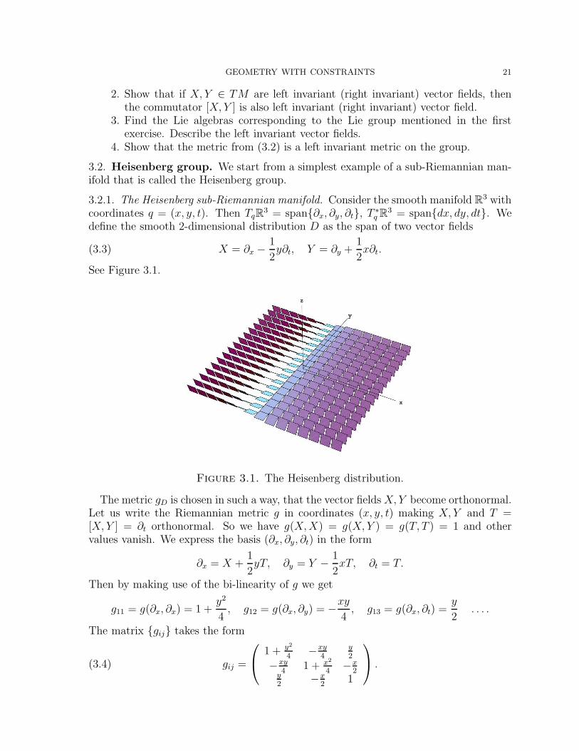
3.2.1. The Heisenberg sub-Riemannian manifold. Consider the smooth manifold R3 withcoordinates q = (x, y, t). Then TqR3 = span∂x, ∂y, ∂t, T ∗q R3 = spandx, dy, dt. Wedefine the smooth 2-dimensional distribution D as the span of two vector fields
(3.3) X = ∂x − 1
2y∂t, Y = ∂y +
1
2x∂t.
See Figure 3.1.
Figure 3.1. The Heisenberg distribution.
The metric gD is chosen in such a way, that the vector fields X, Y become orthonormal.Let us write the Riemannian metric g in coordinates (x, y, t) making X, Y and T =[X, Y ] = ∂t orthonormal. So we have g(X, X) = g(X, Y ) = g(T, T ) = 1 and othervalues vanish. We express the basis (∂x, ∂y, ∂t) in the form
∂x = X +1
2yT, ∂y = Y − 1
2xT, ∂t = T.
Then by making use of the bi-linearity of g we get
g11 = g(∂x, ∂x) = 1 +y2
4, g12 = g(∂x, ∂y) = −xy
4, g13 = g(∂x, ∂t) =
y
2. . . .
The matrix gij takes the form
(3.4) gij =
1 + y2
4−xy
4y2
−xy4
1 + x2
4−x
2y2
−x2
1
.
22 IRINA MARKINA
Notice that det g = 1. It implies that the volume form in H1 is given by the standardLebesgue measure in R3: dx ∧ dy ∧ dt.
The distribution D is bracket generating of step 2 since [X, Y ] = ∂t := T and TqR3 =spanX, Y, T. Moreover, the distribution is strongly bracket generating and we will beinterested in normal geodesics only (by Theorem 2.3). The dual basis to X, Y, T is
dx, dy, ω = dt− 1
2xdy +
1
2ydx.
(Verify it!) The form ω is the annihilator of the distribution D and D⊥ = spanω. Wecan also define the distribution D as D = ker(ω).
To find the normal geodesics on the Heisenberg group we write λ = ξdx + ηdy + θdtfor any co-vector λ. Since the basis X, Y is orthonormal, the Hamiltonian function is
H(q,λ) =1
2
(〈λ, X〉2 + (〈λ, Y 〉2
)=
1
2
((ξ − 1
2θy)2 + (η +
1
2θx)2
).
The Hamiltonian system and the initial conditions are
(3.5)
x = ξ − 12θy
y = η + 12θx
t = 12(ηx− ξy) + 1
4θ(x2 + y2)
ξ = −12ηθ − 1
4θx
η = −12ξθ − 1
4θy
θ = 0,
x = y = t = 0,
ξ = ξ0, η = η0, θ = θ0.
We need projections of the bi-characteristic of H onto R3, therefore, we try to reduce theHamiltonian system to a system containing only the variables (x, y, t). We differentiate
the first two equations and replace ξ and η from the fourth and fifth equations. It gives
(3.6)
x = −θ0y
y = θ0x,or
(xy
)= θ0
(0 −11 0
)(xy
).
Then multiplying the fist equation by y and the second by x we notice that the thirdequation is equivalent to the condition
(3.7) t(s) =1
2(x(s)y(s)− y(s)x(s)).
The solution γ(s) =(x(s), y(s), t(s)
)is
(3.8)
x(s) = ξ0|θ0| sin(|θ0|s)− η0
|θ0|(cos(|θ0|s)− 1),
y(s) = − ξ0|θ0|(cos(|θ0|s)− 1)− η0
|θ0| sin(|θ0|s),t(s) =
(ξ20+η20)
2|θ0|2 (|θ0|s− sin(|θ0|s)),if θ0 .= 0
and
(3.9) x(s) = ξ0s, y(s) = η0s, t(s) = 0, if θ0 = 0.
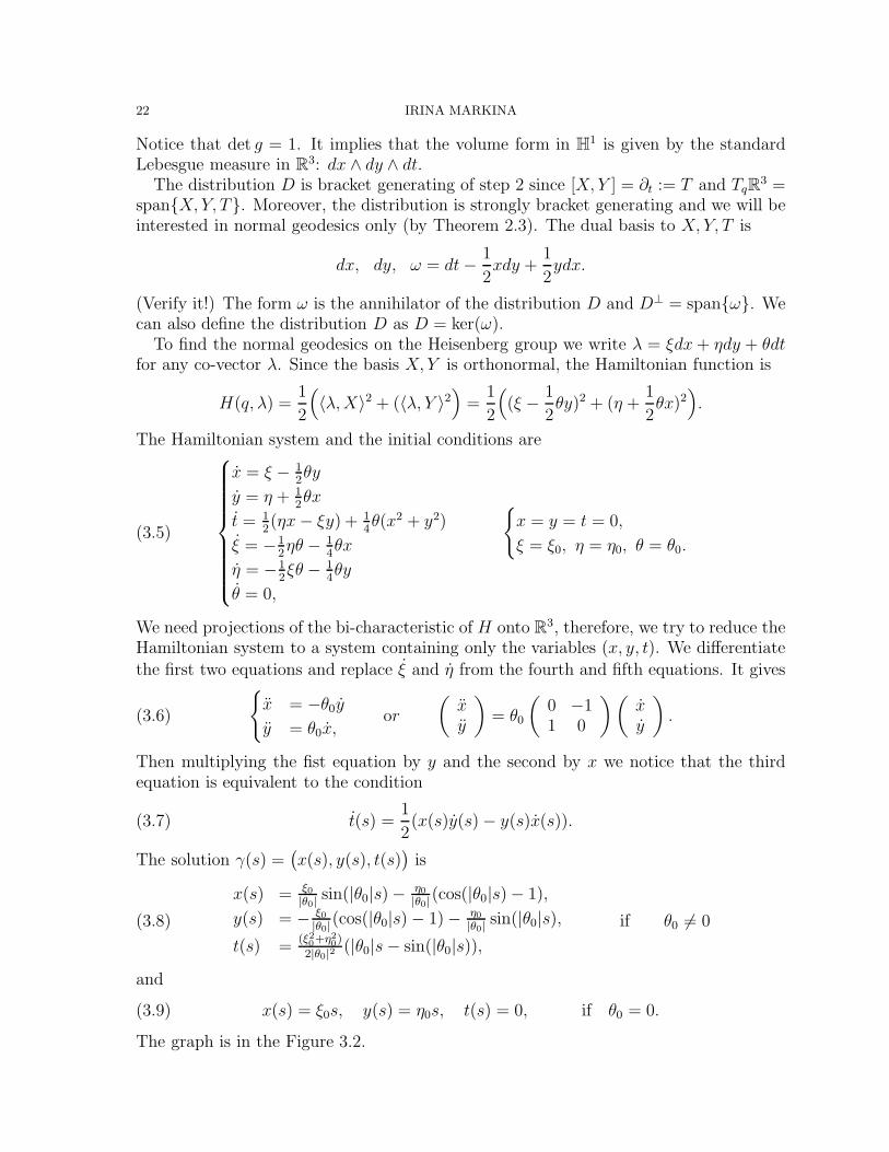
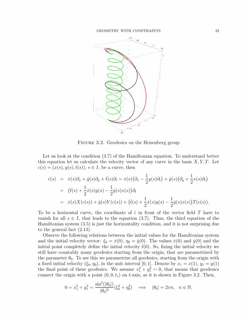
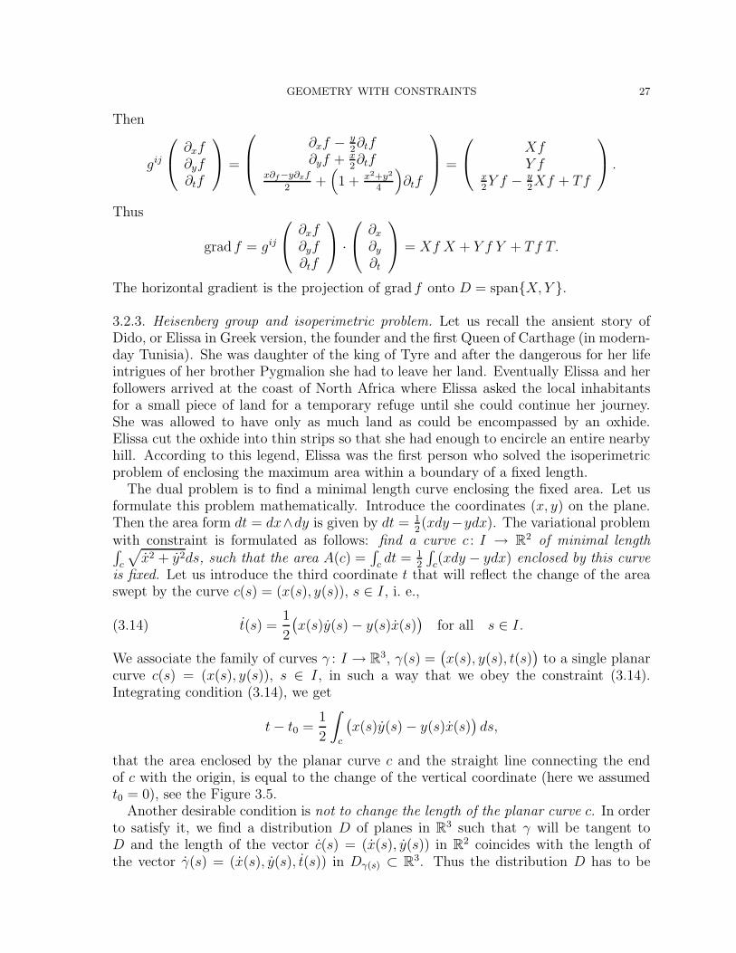
The graph is in the Figure 3.2.
GEOMETRY WITH CONSTRAINTS 23
Figure 3.2. Geodesics on the Heisenberg group
Let us look at the condition (3.7) of the Hamiltonian equation. To understand betterthis equation let us calculate the velocity vector of any curve in the basis X, Y, T . Letc(s) = (x(s), y(s), t(s)), s ∈ I, be a curve, then
c(s) = x(s)∂x + y(s)∂y + t(s)∂t = x(s)(∂x − 1
2y(s)∂t
)+ y(s)
(∂y +
1
2x(s)∂t
)+
(t(s) +
1
2x(s)y(s)− 1
2y(s)x(s)
)∂t
= x(s)X(c(s)) + y(s)Y (c(s)) +(t(s) +
1
2x(s)y(s)− 1
2y(s)x(s)
)T (c(s)).
To be a horizontal curve, the coordinate of c in front of the vector field T have tovanish for all s ∈ I, that leads to the equation (3.7). Thus, the third equation of theHamiltonian system (3.5) is just the horizontality condition, and it is not surprising dueto the general fact (2.13).
Observe the following relations between the initial values for the Hamiltonian systemand the initial velocity vector: ξ0 = x(0), η0 = y(0). The values x(0) and y(0) and theinitial point completely define the initial velocity t(0). So, fixing the initial velocity westill have countably many geodesics starting from the origin, that are parametrized bythe parameter θ0. To see this we parametrize all geodesics, starting from the origin witha fixed initial velocity (ξ0, η0), in the unit interval [0, 1]. Denote by x1 = x(1), y1 = y(1)the final point of these geodesics. We assume x2
1 + y21 = 0, that means that geodesics
connect the origin with a point (0, 0, t1) on t-axis, as it is shown in Figure 3.2. Then,
0 = x21 + y2
1 =sin2(|θ0|)|θ0|2 (ξ2
0 + η20) =⇒ |θ0| = 2πn, n ∈ N.
24 IRINA MARKINA
The corresponding value of t1 is 14(ξ2
0 + η20). The complete discription of geodesics on
the Heisenberg group can be found in [18, 61, 71].The geodesics (3.8) (3.9) are local length minimizers by Theorem 2.3. The length of
a geodesic γ : I = [0, T ]→ R3 is
length(γ) =
∫ T
0
(x(s)2 + y(s)2)1/2ds = (ξ20 + η2
0)1/2T.
If there are several geodesics connecting the origin with another point q then the timeminimizing curve will be the curve realizing the Carnot-Caratheodory distance betweenthe origin and q.
3.2.2. Heisenberg sub-Riemannian manifold as a Lie group. Let us consider the followingnon-commutative group on the smooth manifold R3. Define the group law for τ =(x, y, t) and q = (x1, y1, t1) by
(3.10) τq = (x, y, t)(x1, y1, t1) = (x + x1, y + y1, t + t1 +1
2(xy1 − x1y)).
As a motivation for this law one can consider the product of (4× 4) real matrices1 x y t0 1 0 y
20 0 1 −x
20 0 0 1
·
1 x1 y1 t10 1 0 y1
20 0 1 −x1
20 0 0 1
=
1 x + x1 y + y1 t + t1 + 1
2(xy1 − x1y)
0 1 0 y+y1
20 0 1 −x+x1
20 0 0 1
that leads to formula (3.10). The identity e of the obtained group has coordinates (0, 0, 0)with respect to this multiplication and the inverse element to (x, y, t) is (−x,−y,−t).The pair, consisting of the smooth manifold R3 and the introduced group law, is calledthe Heisenberg group and is denoted by H1. This group law defines the left translation:lτ (q) = τq. The left translation lτ has the differential written in coordinates (x, y, t) as
dlτ =
1 0 00 1 0−1
2y 1
2x 1
.
The action of dlτ on the basis (∂x, ∂y, ∂t) that coincides with (X, Y, T ) at e gives the basis(X, Y, T ) at τ . We conclude that the basis (X, Y, T ) is just the basis of left invariantvector fields on the group H1. They form the famous Heisenberg algebra h1 which is bydefinition a 3-dimensional Lie algebra with only one non-trivial commutator: [X, Y ] = Tand all other vanishing commutators. We use the identification of the Lie algebra of left-invariant vector fields with TeH1. The exponential map is a global diffeomorphism [40]in this case and the coordinates on the group H1 are of the first kind given by
H1 $ q = (x, y, t) = exp(xX + yY + tT ), xX + yY + tT ∈ h1.
GEOMETRY WITH CONSTRAINTS 25
The inverse map restores the group multiplication law from the commutation relations ofthe Heisenberg algebra in the following way. Let V = xX+yY +tT , V1 = x1X+y1Y +t1Tand τ = exp(V ), q = exp(V1), then by the Baker-Campbell-Hausdorff formula (8.1)(BCH-formula for short) we obtain
τq = exp(V ) exp(V1) = exp(V + V1 +1
2[V, V1] + ...)
= exp((x + x1)X + (y + y1)Y + (t + t1)T +
1
2(xy1 − x1y)T
)=
(x + x1, y + y1, t + t1 +
1
2(xy1 − x1y)
),
that coincides with (3.10).There is a norm ‖ · ‖H1 on the group H1 which is a direct analogue of the Euclidean
norm in R3. It is defined by
(3.11) ‖q‖H1 =((
x2 + y2)2
+ t2)1/4
.
If we stretch the basic elements X and Y of the Heisenberg algebra by a number s > 0,then the bi-linearity of the commutators implies [sX, sY ] = s2T . Making use of theBCH-formula we get the dilatation δs on the group:
(3.12) δs(τ) = δs(x, y, t) = (sx, sy, s2t).
This dilation, which is called the homogeneous dilation is compatible with the norm inthe sense that the norm becomes a homogeneous function:
‖δs(τ)‖H1 = ‖(sx, sy, s2t)‖H1 = s‖τ‖H1.
Compare this situation with the Euclidean norm and the usual dilation in R3!The Heisenberg distance function dH1 is
dH1(τ, q) = ‖τ−1q‖H1.
By Exercise (2), the Heisenberg distance dH1 and the Carnot-Caratheodory distance dc−c
are equivalent.
Example 5. Let us show that the Heisenberg distance and the Euclidean distance dE
are not equivalent, even locally in R3. Take two points e = (0, 0, 0) and q = (0, 0, t).Then
dH1(e, q) =√|t|, dE(e, q) = |t|,
that shows non-equivalence of the distance functions. This also proves that the metricspaces (R3, dE) and (R3, dH1) are not equivalent. But the topological spaces (R3, τE) and(R3, τH1) are equivalent since any Heisenberg ball contains the Euclidean ball and viceversa.
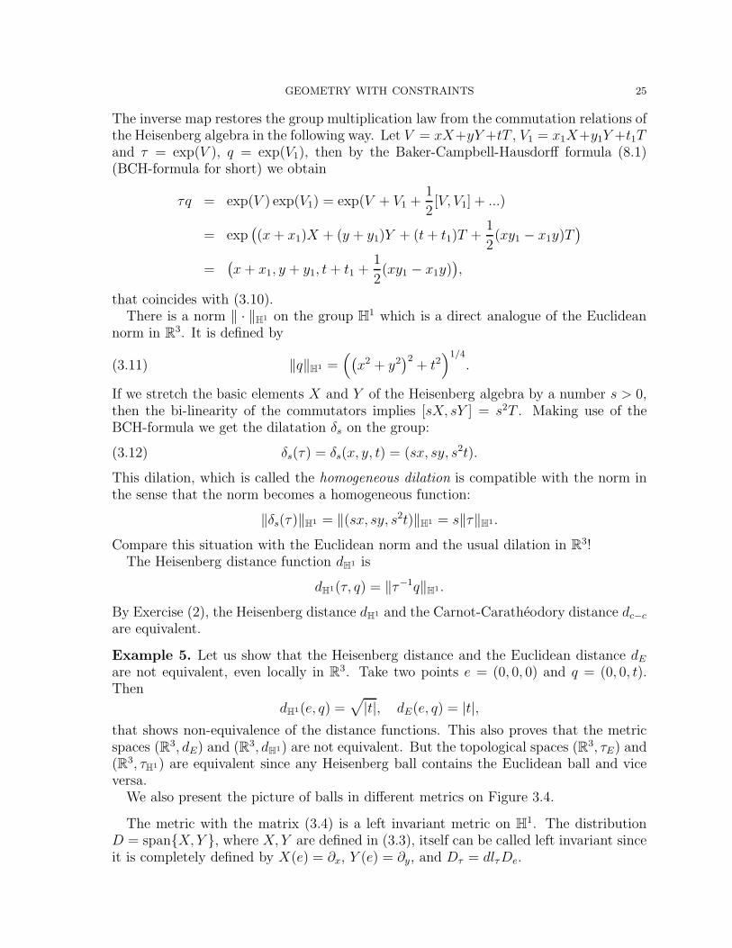
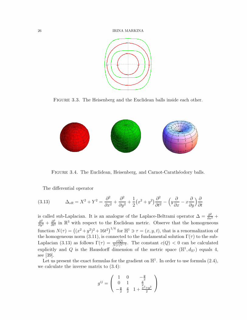
We also present the picture of balls in different metrics on Figure 3.4.
The metric with the matrix (3.4) is a left invariant metric on H1. The distributionD = spanX, Y , where X, Y are defined in (3.3), itself can be called left invariant sinceit is completely defined by X(e) = ∂x, Y (e) = ∂y, and Dτ = dlτDe.
26 IRINA MARKINA
!1.0 !0.5 0.5 1.0
!1.0
!0.5
0.5
1.0
Figure 3.3. The Heisenberg and the Euclidean balls inside each other.
Figure 3.4. The Euclidean, Heisenberg, and Carnot-Caratheodory balls.
The differential operator
(3.13) ∆sR = X2 + Y 2 =∂2
∂x2+
∂2
∂y2+
1
2
(x2 + y2
) ∂2
∂t2−(y∂
∂x− x
∂
∂y
) ∂
∂t
is called sub-Laplacian. It is an analogue of the Laplace-Beltrami operator ∆ = ∂2
∂x2 +∂2
∂y2 + ∂2
∂t2in R3 with respect to the Euclidean metric. Observe that the homogeneous
function N(τ) =((x2 +y2)2 +16t2
)1/4for H1 $ τ = (x, y, t), that is a renormalization of
the homogeneous norm (3.11), is connected to the fundamental solution Γ(τ) to the sub-
Laplacian (3.13) as follows Γ(τ) = c(Q)N(τ)Q−2 . The constant c(Q) < 0 can be calculated
explicitly and Q is the Hausdorff dimension of the metric space (H1, dH1) equals 4,see [39].
Let us present the exact formulas for the gradient on H1. In order to use formula (2.4),we calculate the inverse matrix to (3.4):
gij =
1 0 −y2
0 1 x2
−y2
x2
1 + x2+y2
2
GEOMETRY WITH CONSTRAINTS 27
Then
gij
∂xf∂yf∂tf
=
∂xf − y2∂tf
∂yf + x2∂tf
x∂f−y∂xf
2+(1 + x2+y2
4
)∂tf
=
XfY f
x2Y f − y
2Xf + Tf
.
Thus
grad f = gij
∂xf∂yf∂tf
· ∂x
∂y
∂t
= Xf X + Y f Y + Tf T.
The horizontal gradient is the projection of grad f onto D = spanX, Y .
3.2.3. Heisenberg group and isoperimetric problem. Let us recall the ansient story ofDido, or Elissa in Greek version, the founder and the first Queen of Carthage (in modern-day Tunisia). She was daughter of the king of Tyre and after the dangerous for her lifeintrigues of her brother Pygmalion she had to leave her land. Eventually Elissa and herfollowers arrived at the coast of North Africa where Elissa asked the local inhabitantsfor a small piece of land for a temporary refuge until she could continue her journey.She was allowed to have only as much land as could be encompassed by an oxhide.Elissa cut the oxhide into thin strips so that she had enough to encircle an entire nearbyhill. According to this legend, Elissa was the first person who solved the isoperimetricproblem of enclosing the maximum area within a boundary of a fixed length.
The dual problem is to find a minimal length curve enclosing the fixed area. Let usformulate this problem mathematically. Introduce the coordinates (x, y) on the plane.Then the area form dt = dx∧dy is given by dt = 1
2(xdy−ydx). The variational problem
with constraint is formulated as follows: find a curve c : I → R2 of minimal length∫c
√x2 + y2ds, such that the area A(c) =
∫cdt = 1
2
∫c(xdy − ydx) enclosed by this curve
is fixed. Let us introduce the third coordinate t that will reflect the change of the areaswept by the curve c(s) = (x(s), y(s)), s ∈ I, i. e.,
(3.14) t(s) =1
2
(x(s)y(s)− y(s)x(s)
)for all s ∈ I.
We associate the family of curves γ : I → R3, γ(s) =(x(s), y(s), t(s)
)to a single planar
curve c(s) = (x(s), y(s)), s ∈ I, in such a way that we obey the constraint (3.14).Integrating condition (3.14), we get
t− t0 =1
2
∫c
(x(s)y(s)− y(s)x(s)
)ds,
that the area enclosed by the planar curve c and the straight line connecting the endof c with the origin, is equal to the change of the vertical coordinate (here we assumedt0 = 0), see the Figure 3.5.
Another desirable condition is not to change the length of the planar curve c. In orderto satisfy it, we find a distribution D of planes in R3 such that γ will be tangent toD and the length of the vector c(s) = (x(s), y(s)) in R2 coincides with the length ofthe vector γ(s) = (x(s), y(s), t(s)) in Dγ(s) ⊂ R3. Thus the distribution D has to be
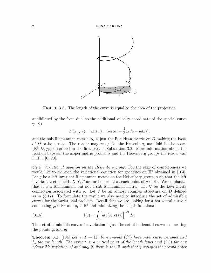
28 IRINA MARKINA
Figure 3.5. The length of the curve is equal to the area of the projection
annihilated by the form dual to the additional velocity coordinate of the spacial curveγ. So
D(x, y, t) = ker(ω) = ker(dt− 1
2(xdy − ydx)),
and the sub-Riemannian metric gD is just the Euclidean metric on D making the basisof D orthonormal. The reader may recognize the Heisenberg manifold in the space(R3, D, gD) described in the first part of Subsection 3.2. More information about therelation between the isoperimetric problems and the Heisenberg groups the reader canfind in [6, 20].
3.2.4. Variational equation on the Heisenberg group. For the sake of completeness wewould like to mention the variational equation for geodesics on H1 obtained in [104].Let g be a left invariant Riemannian metric on the Heisenberg group, such that the leftinvariant vector fields X, Y, T are orthonormal at each point of q ∈ H1. We emphasizethat it is a Riemannian, but not a sub-Riemannian metric. Let ∇ be the Levi-Civitaconnection associated with g. Let J be an almost complex structure on D definedas in (3.17). To formulate the result we also need to introduce the set of admissiblecurves for the variational problem. Recall that we are looking for a horizontal curve cconnecting q0 ∈ H1 and q1 ∈ H1 and minimizing the length functional
(3.15) l(c) =
∫c
[g(c(s), c(s))
]1/2
ds.
The set of admissible curves for variation is just the set of horizontal curves connectingthe points q0 and q1.
Theorem 3.1. [104] Let γ : I → H1 be a smooth (C2) horizontal curve parametrizedby the arc length. The curve γ is a critical point of the length functional (2.3) for anyadmissible variation, if and only if, there is κ ∈ R such that γ satisfies the second order
GEOMETRY WITH CONSTRAINTS 29
ordinary differential equation
(3.16) ∇γ γ + 2κJ(γ) = 0.
This result was recently extended to higher dimensional Heisenberg groups [103]. Theparameter κ is called the curvature of the sub-Riemannian geodesic γ since the projectionof γ to R2 is a curve with the curvature κ. The value κ = 0 corresponds to straightlines parallel to R2.
3.2.5. Heisenberg algebra and Clifford module. Before we finish to discuss the Heisenberggroup and continue with its generalizations, we want to show that the commutationrelations of the Heisenberg algebra induce a natural metric on the Heisenberg groupunder an additional condition. Let us use the notations: X, Y, T for the basis of theHeisenberg algebra h1, U = spanX, Y , V = spanT, and h1 = U ⊕ V . The one-dimensional vector space V is naturally isomorphic to R1 by fixing the basis element T .Therefore, V possesses the metric, such that the length |T | = 1. Thus, V becomes anormed vector space, and therefore, a metric space.
The commutator [·, ·] on the Heisenberg algebra h1 produces a bi-linear skew sym-metric form 0(·, ·) : U → V by 0(u1, u2) := [u1, u2], u1, u2 ∈ U . Let J be an almostcomplex structure on U , that is, a linear map J : U → U , such that
(3.17) J2 = −1, and J(X) = −Y, J(Y ) = X.
Observe that J is compatible with the commutator structure in the sense that thebrackets are invariant under the transformation J . We have
0(JX, JY ) = [JX, JY ] = [X, Y ]
for the basis of U , and thus, for any vector from U . Verify, that −J also possesses thesame properties.
The skew symmetric bi-linear form 0 and the compatible almost complex structure Jdefine a symmetric bi-linear form g(·, ·) : U × U → V by g(Z, W ) = 0(JZ, W ). Indeed,linearity is obvious and symmetry follows from
g(Z, W ) = 0(JZ, W ) = 0(JJZ, JW ) = −0(Z, JW ) = 0(JW, Z) = g(W, Z).
On the basis elements of U we get
g(X, X) = 0(JX, X) = T, g(Y, Y ) = 0(JY, Y ) = T, g(X, Y ) = 0.
Recalling that we use the isomorphism V with R1, we conclude that g is a metric makingX, Y orthonormal. Notice, that J generates a positive definite metric, but −J producesa negative definite metric.
Consider now the commutator as an adjoint map adX : U → V : adX(Z) = [X, Z],(for the definition of the adjoint map and details see Appendix A, Subsection 8.3). ThenadX : (ker(adX))⊥ → V is an isomorphism, and moreover, it is an isometry, since thelength 1 basis element Y is mapped to the length 1 basis element T . The same holdsfor adY . In the construction here we used the almost complex structure J . The choiceof −J leads to a negative definite metric and the adjoint map produces anti-isometries.
The triplet(U, J, (·, ·)) is isomorphic to the set of complex numbers
(C, i, ·) (with
usual multiplication “·” and the imaginary unit i), and which is the first non-trivialrepresentation of the real Clifford algebra with two generators (1, i).
30 IRINA MARKINA
Exercises.
1. Show that the Carnot-Caratheodory distance function is homogeneous with re-spect to dilation (3.12).
2. Show that any two homogeneous with respect to the dilation (3.12) distancefunctions d1 and d2 are equivalent on the Heisenberg group; that is, there are
constants C, C > 0, such that
Cd1(τ, q) ≤ d2(τ, q) ≤ Cd1(τ, q), τ, q ∈ H1.
3. Verify that the Heisenberg distance function dH1 is symmetric and satisfies thetriangle inequality. If you did not succeed see [72].
4. Show that geodesics (3.8), (3.9) are invariant under the left translation definedby the multiplication (3.10).
5. Prove that all geodesics on the Heisenberg group can be obtained by left trans-lations of geodesics (3.8) and (3.9) starting from e = (0, 0, 0).
3.3. H-type groups. The Heisenberg type groups (H-type for shortness) were intro-duced by A. Kaplan [61] and have been studied extensively by many mathematicians,see for instance [19, 24, 29, 62, 71, 102].
The Heisenberg-type groups H are generalizations of the Heisenberg group in the sensethat adX defines an isometry from the center of the Lie algebra to the complement ofits kernel. To define an H-type groups we present a Lie algebra and then by makinguse of the BCH-formula (8.1) we get a simply connected group. We start from a vectorspace h, endowed with a commutator [·, ·] and an inner product (·, ·). We suppose thatthe commutator defines the decomposition
h = U ⊕ V, [U, U ] ⊆ V, [U, V ] = [V, V ] = 0,and, moreover, this decomposition is orthogonal with respect to the inner product. Thenext assumption is compatibility between [·, ·], (·, ·), and an almost complex structure.We assume that there is a map J : V → End(U), that satisfies
(3.18) (JTX, Y ) = (T, [X, Y ]), for any X, Y ∈ U, and any T ∈ V.
This immediately implies the skew-symmetry of JT for any T ∈ V :
(3.19) J trT = −JT .
Here J trT denotes dual map to JT . For any element X ∈ U the adjoint map adX =
[X, ·] : U → V gives the decomposition
U = ker(adX)⊕ (ker(adX)
)⊥.
We say that the Lie algebra(h, [·, ·], (·, ·)) is of H-type if for any X ∈ U , (X, X) = 1 the
map
adX :(ker(adX)
)⊥ → V
is an isometry onto V . The last condition is equivalent to
(3.20) J2T = −|T |2 Id, for all T ∈ V,
GEOMETRY WITH CONSTRAINTS 31
where Id denotes the identity mapping in End(U) [29]. The conditions (3.19), (3.20)imply
(3.21) JT JT ′ + JT ′JT = −2(T, T ′) Id, for all T, T ′ ∈ V,
see [29]. When there exists a linear mapping J : V → End(U) satisfying (3.19) and (3.20)or (3.21), U is called the Clifford module over V . The relation between H-type groupsand Clifford modules was carefully studied in [29].
In this part of the lectures we present the most beautiful class of H-type groups thatis related to division algebras of real, complex, quaternion and octonion numbers. TheH-type groups related to division algebras were studied in [19], where the parametricformulas of geodesics and other questions also were obtained.
Definition 17. The algebra h satisfies the J2 condition if, whenever X ∈ U and T, T ′ ∈V with (T, T ′) = 0, then there exists T ′′ ∈ V , such that
(3.22) JT JT ′X = JT ′′X.
The authors of [29] presented a classification of H-type algebras satisfying the J2
condition. Denote by hn0 the Euclidean n-dimensional space, by hn
1 the n-dimensionalHeisenberg algebra, by hn
3 the n-dimensional quaternion H-type algebra, and by h17 the
octonion H-type algebra. The lower index corresponds to the topological dimension ofV and the upper index reflects the real, complex, quaternion and octonion topologicaldimensions of U .
Theorem 3.2 ([29]). Suppose that h is an H-type algebra satisfying the J2 condition.Then h is isometrically isomorphic to hn
0 , hn1 , hn
3 or to h17.
Before we describe the general construction of groups Hn0 , Hn
1 , Hn3 , and H1
7, we wouldlike to remind the Cayley-Dickson construction of division algebras R (real numbers), C(complex numbers), Q (quaternion numbers), and O (octonion numbers). The Cayley-Dickson construction explains why each algebra fits neatly inside the next one. Recallthat the division algebra means that each non-zero element has a unique inverse. TheCayley-Dickson construction is given nicely in [8].
The complex number, as well known, can be thought of as a pair (a, b) of real numbersa, b ∈ R. We define the conjugate to a real number as a∗ = a and the conjugate to thepair as
(3.23) (a, b)∗ = (a∗,−b).
Then the Cayley-Dickson product is defined by
(3.24) (a, b)(c, d) = (ac− db∗, a∗d + cb).
Now we can think of a pair (a, b) as a quaternion, where a, b ∈ C. The conjugate isdefined as in (3.23) and the product as in (3.24). We obtain the quaternion numbersQ that form a non-commutative algebra with respect to (3.24). Finally, we define anoctonion as a pair (a, b) with a, b ∈ Q, the conjugate as in (3.23), and the product (3.24).The octonions with the multiplication (3.24) form a non-commutative, non-associativealgebra. Actually, we can continue the Cayley-Dickson construction doubling thedimension and getting a bit worse algebras. First we loose the fact that every element
32 IRINA MARKINA
is its own conjugate, then we loose commutativity, associativity, and finally we loose thedivision algebra property. An algebra possesses a division property if
xy = 0 implies x = 0 or y = 0.
3.3.1. Constructions of H-types groups related to division algebras. Using the Cayley-Dickson product, we first describe the following groups: Euclidean n-dimensional spaceHn
0 = Rn, the n-dimentional Heisenberg group Hn1 , the n-dimentional quaternion H-type
group Hn3 , and the octonion H-type group H1
7. The corresponding Lie algebras hn0 , hn
1 ,hn
3 , and h17 are infinitesimal representations of these groups.
We want to note that the definitions of H17 and h1
7 differ from the ones in [29]. Inour construction we used the octonion product which is not associative, therefore, it cannot give a Clifford algebra, where the product is associative by definition. The groupcorresponding to the classification of Theorem 3.2 is essentially the same as we present,where the product of octonions has to be changed to an associative multiplication,presented in [29].
The Euclidean space. The group Hn0 =
(Rn, +) is a trivial example of an H-type
group. We have the identifications
hn0 = TeRn = Rn = span∂x1, . . . , ∂xn.
Left invariant vector fields are linear combinations of (∂x1 , . . . , ∂xn) with constant co-efficients. The exponential map is the identity map. Since all commutators [∂x1 , ∂xn ]vanish, we get
hn0 = U ⊕ V, U = Rn, V = 0.
The Heisenberg group Hn1 . We start from n = 1, and then generalize it to an
arbitrary n = 2k, k ∈ N. Complex numbers considered as a vector space have 2 basisvectors that we call unities, since their squares have absolute value 1:
real 1 = (1, 0), 12 = 1, and imaginary i = (0, 1), i2 = −1.
Take a complex number z = (x1, x2), x1, x2 ∈ R, and a real number t. Define a newnon-commutative law between the elements τ = [z, t], q = [z′, t′] ∈ C× R by
(3.25) τq = [z, t][z′, t′] = [z + z′, t + t′ +1
2(zi) · z′],
where firstly we take the Cayley-Dickson product zi = (x1, x2)(0, 1) and then the innerproduct “·” of vectors z, z′ ∈ R2. If we use the representation of i as the (2× 2) matrix
i =
[0 1
−1 0
],
then the group law can be written as
τq = [z, t][z′, t′] = [z + z′, t + t′ +1
2(iz) · z′].
Using the algebraic form of a complex number z = x1 + ix2 = Rez + i Imz, we canwrite (3.25) in the form
τq = [z, t][z′, t′] = [z + z′, t + t′ +1
2Im(z∗z′)],
GEOMETRY WITH CONSTRAINTS 33
where z∗z′ is the Cayley-Dickson product of z∗ by z′. The non-commutativity of thenew multiplication law in C× R is seen for the last variable t ∈ R. One-dimensionalityof the second slot of coordinates reflects the existence of only one imaginary unit. Thereader easily recognizes the Heisenberg group H1 with the multiplication law (3.10).
In order to present an n-dimensional analogue of the Heisenberg group we take twon-dimensional vectors of complex numbers w = (z1, . . . , zn), w′ = (z′1, . . . , z
′n), zl =
x1l + ix2l, z′l = (x1l)′ + i(x2l)′, l = 1, . . . , n. The matrix i is changed to a block diagonalmatrix J = diag i with n matrices i on the diagonal. The multiplication law betweenthe elements τ = [w, t] and q = [w′, t′] ∈ Cn × R is transformed into the following one
τq = [w, t][w′, t′] = [w + w′, t + t′ +1
2
n∑l=1
(zli) · z′l] = [w + w′, t + t′ +1
2(Jw) · w′]
= [w + w′, t + t′ +1
2Im(w∗w′)],
where w∗w′ =∑n
l=1 z∗l z′l. The unit element is e = (0, 0) and (−w − t) = (w, t)−1 is the
inverse element to (w, t).The Heisenberg algebra hn
1 , n = 2k, k ∈ N, of left invariant vector fields is obtained asin one dimensional case by translation of the basis vectors ∂x1l, ∂x2l , ∂tn
l=1 at the unityby dlτ . We get
(3.26) X1l = ∂x1l− 1
2x2l∂t, X2l = ∂x2l
+1
2x1l∂t, l = 1, . . . , n and T = ∂t.
Let us introduce the notations U = spanX1l, X2lnl=1, V = spanT. Since [X1l, X2l] =
T and other commutators vanish, we get hn1 = U ⊕ V . Let the inner product (·, ·) in hn
1
be such that basis vector fields become orthonormal. The condition (3.18) holds due tothe commutation relations. The endomorphism JT is represented by the matrix J, whichpossesses properties (3.19), (3.20). The J2 condition holds trivially, since dim V = 1.The space (U, J, (·, ·)) is isomorphic to the space of complex numbers (Cn, i, ·) (with usualmultiplication “·”), which is the simplest example of a Clifford algebra with generators1, i.
Quaternion group Hn3 . As previously, we start from the one-dimensional case, and
then consider its multidimensional analogue. Quaternion numbers, which we think of aspairs of complex numbers, have one real unity 1 = (1, 0), 12 = 1, and three imaginaryunits
i1 = (i, 0), i2 = (0, 1), i3 = (0, i), such that i21 = i22 = i23 = i1i2i3 = −1.
The Cayley-Dickson product is no longer commutative, for example,
(3.27) i1i2 = −i2i1 = −i3, i2i3 = −i3i2 = −i1, i3i1 = −i1i3 = −i2.
In order to construct the quaternion H-type group H13, we take a quaternion q = (z1, z2),
z1, z2 ∈ C, and three real numbers t1, t2, t3 that reflects the three dimensional nature ofthe space of the imaginary quaternions. Define a new non-commutative law between the
34 IRINA MARKINA
elements h = [q, t1, t2, t3] ∈ Q× R3 and p = [q′, t′1, t′2, t
′3] ∈ Q× R3 by
hp = [q, t1, t2, t3][q′, t′1, t
′2, t
′3]
= [q + q′, t1 + t′1 +1
2(qi1) · q′, t2 + t′2 +
1
2(qi2) · q′, t3 + t′3 +
1
2(qi3) · q′],(3.28)
where qik, k = 1, 2, 3 is the Cayley-Dickson product for the quaternions and “·” is theinner product in R4. As in the case of the Heisenberg group we can use the matrixrepresentation of the imaginary units(3.29)
i1 =
0 −1 0 01 0 0 00 0 0 −10 0 1 0
, i2 =
0 0 −1 00 0 0 11 0 0 00 −1 0 0
, i3 =
0 0 0 −10 0 −1 00 1 0 01 0 0 0
,
and rewrite the group law (3.28) in the form
hp = [q + q′, t1 + t′1 +1
2(i1q) · q′, t2 + t′2 +
1
2(i2q) · q′, t3 + t′3 +
1
2(i3q) · q′].
Using the imaginary units we can represent a quaternion q in the algebraic form as
q = α + i1β + i2γ + i3δ = α + i1Im1q + i2Im3q + i3Im3q.
Then the multiplication law (3.28) admits the form
hp = [q, t1, t2, t3][q′, t′1, t
′2, t
′3]
= [q + q′, t1 + t′1 +1
2Im1(q
∗ q′), t2 + t′2 +1
2Im2(q
∗ q′), t3 + t′3 +1
2Im3(q
∗ q′)],(3.30)
where q∗ q′ is the Cayley-Dickson product of q∗ by q′.To give an n-dimensional analogue of the quaternion H−type group, we take the n-
dimensional vectors of quaternion numbers w = (q1, . . . , qn), w′ = (q′1, . . . , q′n). Each of
the matrices im, m = 1, 2, 3, is changed to the block diagonal matrix Jm = diag im withn (4×4)-dimensional matrices im on the main diagonal. The multiplication law betweenthe elements h = [w, t1, t2, t3], p = [w′, t′1, t
′2, t
′3] ∈ Qn × R3 is
hp = [w, t1, t2, t3][w′, t′1, t
′2, t
′3]
= [w + w′, t1 + t′1 +1
2
n∑l=1
(qli1)q′l, t2 + t′2 +
1
2
n∑l=1
(qli2)q′l, t3 + t′3 +
1
2
n∑l=1
(qli3)q′l]
= [w + w′, t1 + t′1 +1
2(J1w) · w′, t2 + t′2 +
1
2(J2w) · w′, t3 + t′3 +
1
2(J3w) · w′]
= [w + w′, t1 + t′1 +1
2Im1(w
∗w′), t2 + t′2 +1
2Im2(w
∗w′), t3 + t′3 +1
2Im3(w
∗w′)],
where w∗w′ =∑n
l=1 q∗l q′l. The unity is e = (0, 0) and the inverse element to (w, t1, t2, t3)is (−w,−t1,−t2,−t3).
The quaternion algebra hn3 , n = 4k, k ∈ N, is the direct sum of U ⊕ V , where
U = span(X11, X21, X31, X41, . . . , X1n, X2n, X3n, X4n)
GEOMETRY WITH CONSTRAINTS 35
with
X1l(w, t) =∂x1l+
1
2
(− x2l∂t1 − x3l∂t2 − x4l∂t3
),
X2l(w, t) =∂x2l+
1
2
(x1l∂t1 + x4l∂t2 − x3l∂t3
),
X3l(w, t) =∂x3l+
1
2
(− x4l∂t1 + x1l∂t2 + x2l∂t3
),
X4l(w, t) =∂x4l+
1
2
(x3l∂t1 − x2l∂t2 + x1l∂t3
),
l = 1, . . . n(3.31)
and w = (q1, . . . , qn) = (x11, x21, x31, x41, . . . , x1 n, x2 n, x3 n, x4 n). The subspace V isspanned by T1, T2, T3 with Tk = ∂tk . The following commutator relations
[X1l, X2l] = T1, [X1l, X3l] = T2, [X1l, X4l] = T3,
[X2l, X3l] = T3, [X2l, X4l] = −T2, [X3l, X4L] = T1,
hold for l = 1, . . . , n and the others vanish. Thus, the condition (3.18) is verifiedwith respect to the inner product making the bases of U and V orthonormal. Theendomorphisms JTm are represented by matrices Jm, m = 1, 2, 3. The J2 conditionholds due to relation (3.27).
Remark 1. If we involve only two imaginary units into the construction, then we obtainthe quaternion H-type group with two dimensional center V . Taking into considerationonly one of the ik, k = 1, 2, 3, we get a group isomorphic to the Heisenberg group Hn
1 .
Octonion H-type group H17. Octonions or Caley numbers, which we think of as
pairs of quaternion numbers, has one real unit 1 = (1, 0), 12 = 1 and 7 imaginary units
j1 = (i1, 0), j2 = (i2, 0), j3 = (i3, 0), j4 = (0, 1), j5 = (0, i1) j6 = (0, i2), j7 = (0, i3),
whose squares equal (−1). The rule of multiplication is presented in Table 9 in Appen-dix B. The product of octonions is not associative, for example,
j1(j2j4) = −j7, (j1j2)j4 = j7.
We take an octonion w = (q1, q2), q1, q2 ∈ Q and 7 real numbers tk, k = 1, . . . , 7, corre-sponding to 7-dimensional space of imaginary octonions. Define a new non-commutativeproduct law for elements h = [w, t] = [w, t1, . . . , t7], p = [w′, t′] = [w′, t′1, . . . , t
′7] ∈ O×R7
by
hp = [w, t][w′, t′] = [w, t1, . . . , t7][w′, t′1, . . . , t
′7]
= [w + w′, t1 + t′1 +1
2(wj1) · w′, . . . , t7 + t′7 +
1
2(wj7) · w′](3.32)
= [w + w′, t1 + t′1 +1
2Im1(w
∗w′), . . . , t7 + t′7 +1
2Im7(w
∗w′)],
where wjm, m = 1, . . . , 7, and w∗w′ are the Cayley-Dickson product and “·” is the innerproduct in R8. As in the previous cases e = (0, 0), (w, t)−1 = (−w,−t).
There is no matrix representation of jk since the multiplication between jk is notassociative, in contrast to the matrix multiplication. Nevertheless, it is possible toassociate a matrix Jm with any imaginary unit jm which will represent the corresponding
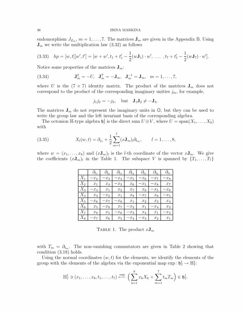
36 IRINA MARKINA
endomorphism JZm, m = 1, . . . , 7. The matrices Jm are given in the Appendix B. UsingJm we write the multiplication law (3.32) as follows
(3.33) hp = [w, t][w′, t′] = [w + w′, t1 + t′1 −1
2(wJ1) · w′, . . . , t7 + t′7 −
1
2(wJ7) · w′].
Notice some properties of the matrices Jm:
(3.34) J2m = −U, JT
m = −Jm, J−1m = Jm, m = 1, . . . , 7,
where U is the (7 × 7) identity matrix. The product of the matrices Jm does notcorrespond to the product of the corresponding imaginary unities jm, for example,
j1j2 = −j3, but J1J2 .= −J3.
The matrices Jm do not represent the imaginary units in O, but they can be used towrite the group law and the left invariant basis of the corresponding algebra.
The octonion H-type algebra h17 is the direct sum U⊕V , where U = span(X1, . . . , X8)
with
(3.35) Xl(w, t) = ∂xl+
1
2
7∑m=1
(xJm)l∂tm , l = 1, . . . , 8,
where w = (x1, . . . , x8) and (xJm)l is the l-th coordinate of the vector xJm. We givethe coefficients (xJm)l in the Table 1. The subspace V is spanned by T1, . . . , T7
∂t1 ∂t2 ∂t3 ∂t4 ∂t5 ∂t6 ∂t7
X1 −x2 −x3 −x4 −x5 −x6 −x7 −x8
X2 x1 x4 −x3 x6 −x5 −x8 x7
X3 −x4 x1 x2 x7 x8 −x5 −x6
X4 x3 −x2 x1 x8 −x7 x6 −x5
X5 −x6 −x7 −x8 x1 x2 x3 x4
X6 x5 −x8 x7 −x2 x1 −x4 x3
X7 x8 x5 −x6 −x3 x4 x1 −x2
X8 −x7 x6 x5 −x4 −x3 x2 x1
Table 1. The product xJm
with Tm = ∂tm . The non-vanishing commutators are given in Table 2 showing thatcondition (3.18) holds.
Using the normal coordinates (w, t) for the elements, we identify the elements of thegroup with the elements of the algebra via the exponential map exp : h1
7 → H17:
H17 $ (x1, . . . , x8, t1, . . . , t7)
exp←−( 8∑
k=1
xkXk +7∑
m=1
tmTm
)∈ h1
7.
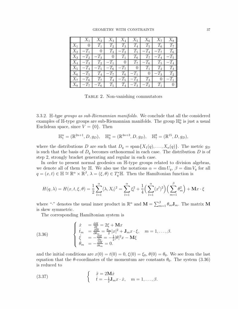
GEOMETRY WITH CONSTRAINTS 37
X1 X2 X3 X4 X5 X6 X7 X8
X1 0 T1 T2 T3 T4 T5 T6 T7
X2 −T1 0 T3 −T2 T5 −T4 −T7 T6
X3 −T2 −T3 0 T1 T6 T7 −T4 −T5
X4 −T3 T2 −T1 0 T7 −T6 T5 −T4
X5 −T4 −T5 −T6 −T7 0 T1 T2 T3
X6 −T5 T4 −T7 T6 −T1 0 −T3 T2
X7 −T6 T7 T4 −T5 −T2 T3 0 −T1
X8 −T7 −T6 T5 T4 −T3 −T2 T1 0
Table 2. Non-vanishing commutators
3.3.2. H-type groups as sub-Riemannian manifolds. We conclude that all the consideredexamples of H-type groups are sub-Riemannian manifolds. The group Hn
0 is just a usualEuclidean space, since V = 0. Then
Hn1 = (R2n+1, D, gD), Hn
3 = (R4n+3, D, gD), H87 = (R15, D, gD),
where the distributions D are such that Dq = spanX1(q), . . . , Xα(q). The metric gD
is such that the basis of Dq becomes orthonormal in each case. The distribution D is ofstep 2, strongly bracket generating and regular in each case.
In order to present normal geodesics on H-type groups related to division algebras,we denote all of them by H. We also use the notations α = dim Uq, β = dim Vq for allq = (x, t) ∈ H ∼= Rα × Rβ, λ = (ξ, θ) ∈ T ∗q H. Then the Hamiltonian function is
H(q,λ) = H(x, t, ξ, θ) =1
2
α∑l=1
〈λ, Xl〉2 =
α∑l=1
ξ2l +
1
4
( α∑l=1
(xl)2)( β∑
m=1
θ2m
)+ Mx · ξ
where “·” denotes the usual inner product in Rα and M =∑β
m=1 θmJm. The matrix Mis skew symmetric.
The corresponding Hamiltonian system isx = ∂H
∂ξ= 2ξ + Mx
tm = ∂H∂θm
= θm
2|x|2 + Jmx · ξ, m = 1, . . . , β.
ξ = −∂H∂x
= −12|θ|2x−Mξ
θm = − ∂H∂tm
= 0.
(3.36)
and the initial conditions are x(0) = t(0) = 0, ξ(0) = ξ0, θ(0) = θ0. We see from the lastequation that the θ-coordinates of the momentum are constants θ0. The system (3.36)is reduced to
x = 2Mxt = −1
2Jmx · x, m = 1, . . . , β.
(3.37)
38 IRINA MARKINA
The solutions of the system (3.37) for θ0 .= 0 arex(s) = 1−cos(2s|θ0|)
2|θ0|2 Mx(0) + sin(2s|θ0|)2|θ0| Id x(0)
tm(s) = (θ0)m|x(0)|24|θ0|2
(s− sin(2s|θ0|)
2|θ0|), m = 1, . . . , β,
(3.38)
where Id is the identity matrix in Rα. If θ0 vanishes, then the geodesics are straightlines starting from (0, 0) with the initial velocity ξ0, θ0 = 0, remaining in the spacet = 0. Analyzing the solutions, we obtain the information about behavior of geodesicssimilar to the Heisenberg group. Projections to any 3-dimensional subspace containingtwo x-coordinates and one t-coordinate give the Heisenberg picture, see Figure 3.2. Thedetail study of this question can be found in [19].
In the work [48] the authors obtained an analogue of the variational equation (3.1)for the H-type group H1
3 = (R7, ρ), where the group law ρ is given by (3.30).
Theorem 3.3. Let γ : [a, b] → H13 be a horizontal curve, parameterized by arc length.
Then γ is a critical point of the functional for the Carnot-Caratheodory distance, ifand only if, there exist numbers κ1, κ2, κ3 ∈ R such that γ satisfies the second orderdifferential equation
(3.39) ∇γ γ − 2∑
m=1,2,3
κmJm(γ) = 0.
Here Jm, m = 1, 2, 3, are almost complex structures given by endomorphisms JTm ,m = 1, 2, 3 in the definition of H1
3. The Levi-Civita connection ∇ is compatible with theextension of the sub-Riemannian metric gD from D onto the entire tangent bundle TH1
3.The question whether there are similar equations for other H-type groups is still open.See an analogue of equation (3.39) in Subsection 5.5.
We also present here formulas for horizontal gradients on groups H, written in theleft invariant basis (X1, . . . , Xα) given in (3.26), (3.31), (3.35) and in the standard basis∂xl, ∂tm, l = 1, . . . ,α, m = 1, . . . , β.
(3.40) gradD = (X1, . . . , Xα) = (gradx +1
2
β∑m=1
(Jmx)∂tm),
with gradx = (∂x1 , . . . , ∂xα).
3.3.3. Action of H-type groups on the Siegel upper half space. Let Cn+1 be the (n + 1)-dimensional complex space. We use the notation z = (z′, zn+1), where z′ = (z1, . . . , zn) ∈Cn. The set
Un = (z1, . . . , zn+1) ∈ Cn+1 : 4Re (zn+1) > |z′|2 =
n∑l=1
|zl|2
defines the Siegel upper half space. Let BC denotes the unit ball in Cn+1:
BC = (w1, . . . , wn+1) ∈ Cn+1 :n+1∑l=1
|wl|2 < 1.
GEOMETRY WITH CONSTRAINTS 39
Then the Cayley transformation
wn+1 =1− zn+1
1 + zn+1, wl =
zl
1 + zn+1, l = 1, . . . , n,
and its inverse
zn+1 =1− wn+1
1 + wn+1
, zl =2wl
1 + wn+1
, l = 1, . . . , n,
show that the unit ball BC and the Siegel upper half space Un are biholomorphicallyequivalent.
Let Qn+1, n + 1 = 4k, k ∈ N, be an (n + 1)-dimensional quaternion vector space overthe field of real numbers. The elements of Qn+1 are (n + 1)-tuples of quaternions that
we denote by q = (q′, qn+1), q′ = (q1, . . . , qn) ∈ Qn, with the norm ‖q‖2 =∑n+1
l=1 q2l . The
Siegel upper half space in Qn+1 can be defined by analogy with the complex case as:
Un = (q1, . . . , qn+1) ∈ Qn+1 : 4Re (qn+1) >n∑
l=1
|ql|2 = |q′|2.
The unit ball BQ in Qn+1 is
BQ = (h1, . . . , hn+1) ∈ Qn+1 :
n+1∑l=1
|hl|2 < 1.
Since the multiplication of quaternions is not commutative there are two forms of Cayleytransformation that give the symmetric geometry. The (left) Cayley transformation,mapping the Siegel upper half space Un onto the unit ball BQ, has the form
qn+1 = (1 + hn+1)−1(1− hn+1) =
(1 + h∗n+1)(1− hn+1)
|1 + hn+1|2 ,
ql = 2hl(1 + hn+1)−1 =
2hl(1 + h∗n+1)
|1 + hn+1|2 ,
for l = 1, . . . , n. The inverse transformation from BQ onto Un is
hl = ql(1 + qn+1)−1 =
ql(1 + q∗n+1)
|1 + qn+1|2 ,
hn+1 = (1− qn+1)(1 + qn+1)−1 =
(1− qn+1)(1 + q∗n+1)
|1 + qn+1|2for l = 1, . . . , n. The Cayley transformation is biholomorphic in the quaternion sense.
Continuing by analogy, we define the Siegel upper half space in O2. We shall consideronly 2-dimensional case of the octonion vector space over the field of real numbers:O2 = o = (o′, o2) : o′, o2 ∈ O with the norm |o|2 = |o′|2 + |o2|2. The Siegel upper halfspace U1 and the unit disk BO can be defined as
U1 = (o′, o2) ∈ O2 : 4Re (o2) > |o′|2,BO = (r′, r2) ∈ O2 : |r′|2 + |r2|2 < 1.
The transformations
o′ = 2r′(1 + r2)−1, o2 = (1 + r2)
−1(1− r2),
40 IRINA MARKINA
map the Siegel upper half space onto the unit ball and the map
r′ = o′(1 + o2)−1, r2 = (1− o2)(1 + o2)
−1
acts from the unit ball to the Siegel upper half space. To verify this we observe that
(xy)∗ = y∗x∗, x−1 =x∗
|x|2 ,
where x is a complex number, a quaternion or an octonion, and xy is the Cayley-Dicksonproduct. Let us denote by (q′, q) an element of one of the above mentioned Siegel upperhalf spaces, and by (h′, h) a point from the corresponding unit ball. Then
|h′|2 = h′(h′)∗ = |q′|2|(1 + q)−1|2,|h|2 = hh∗ = |1− q|2|(1 + q)−1|2,
and
|h′|2 + |h|2 = (|q′|2 + |1− q|2)|(1 + q)−1|2 < 1.
Since |(1 + q)−1|2 = |(1 + q)|−2, we have
|q′|2 + |1− q|2 = |q′|2 + 1 + |q|2 − 2Re (q) < |(1 + q)|2 = 1 + |q|2 + 2Re (q),
that yields |q′|2 < 4Re (q).Let K be one of the following spaces Cn+1, Hn+1 or O2. We denote by p = (q′, q) a
point from the Siegel upper half space Un of K. The boundary of the space Un is
∂Un = (q′, q) ∈ K : 4Re (q) = |q′|2 =n∑
l=1
|ql|2.
We mention here three automorphisms of the domain Un: dilation, rotation and trans-lation.
Dilation. Let p = (q′, q) ∈ Un. For every positive number δ we define a dilation δs(p)by
δs(p) = δs(q′, q) = (sq′, s2q).
The non-isotropy of the dilation comes from the definition of Un.Rotation. For every unitary linear transformation U that acts on Cn, Hn or O, we
define the rotation Rot(p) on Un by
Rot(p) = Rot(q′, q) = (U(q′), q).
Both the dilation and the rotation are extended to mappings on the boundary ∂Un.Translation. We use the notation H for the H-type groups Hn
1 , Hn3 , H1
7. To everyelement [w, t] of H we associate the following affine self-map of Un. Notice that it is aholomorphic map for the cases Cn+1, Qn+1. This map is the action on the left of thegroup H on Un:
(3.41) [w, t].(q′, q) %→ (q′ + w, q +|w|24
+1
2w∗q′ + i · t).
Here i · t =∑β
l=1 iktk. This mapping preserves the level sets, given by the function
(3.42) r(p) = 4Re (q)− |q′|2.
GEOMETRY WITH CONSTRAINTS 41
In fact, since |q′ + w|2 = |q′|2 + |w|2 + 2Re (w∗q1), we obtain
4Re (q +|w|24
+1
2w∗q′)− |q′ + w|2 = 4Re (q)− |q′|2.
Hence, the transformation (3.41) maps Un onto itself and preserves the boundary ∂Un.Let us check that the mapping (3.41) defines an action of the group H on the space Un.
If we compose the mappings (3.41), corresponding to elements [w, t] and [ω, s] ∈ H, weget
(3.43) [w, t].([ω, s].(q′, q)
)=(w+ω+q′, q+
|w|24
+|ω|24
+1
2(w+ω)∗q′+
1
2w∗ω+i·(s+t)
).
On the other hand, the transformation corresponding to the element [w, t][ω, s] is
(3.44) [w, t][ω, s].(q′, q) =(w+ω+q′, q+
|w + ω|24
+1
2(w+ω)∗q′+
1
2i·Im w∗ω+i·(s+t)
).
Observing that
|w + ω|24
+1
2i · Im w∗ω =
|w|24
+|ω|24
+1
2Re (w∗ω) +
1
2i · Im w∗ω =
|w|24
+|ω|24
+1
2w∗ω,
we conclude that (3.43) and (3.44) give the same result. Thus, (3.41) gives us a real-ization of H as a group of affine (q-holomorphic) bijections of Un. We can identify theelements of Un with the boundary via its action at the origin
h(0) = [w, t].(0, 0) %→ (w, |w|2 + i · t),where h = [w, t]. Thus,
H $ [w, t] %→ (w, |w|2 + i · t) ∈ ∂Un.
We may use the following coordinates (q′, t, r) = (q′, t1, . . . , tdim V2, r) on Un:
Un $ (q′, q) = (q′, t, r), where tk = Imkq, k = 1, . . . , β, r = r(q′, q) = 4Re (q)− |q′|2.If 4Re (q) = |q′|2, then we get coordinates on the boundary ∂Un of the Siegel upper halfspace
∂Un $ (q′, q) = (q′, t1, . . . , tdimV2),
where tk are as above and r = r(q′, q) = 0.
3.4. Carnot groups. The next example includes simply connected Lie groups G whoseLie algebras are the direct sum of their subspaces
g = V1 ⊕ V2 ⊕ . . . Vm,
such that [V1, Vk] = Vk+1, k = 1, 2, . . . , m− 1, and [V1, Vm] = 0. Since the commutatorshave finite length the algebras and the groups are nilpotent. The Lie algebras are alsograded: [Vl, Vk] ⊆ Vl+k and stratified
0 ∈ V1 ⊂ V1 ⊕ V2 ⊂ . . . ⊂ ⊕mk=1Vk.
Such kind of groups received the name the Carnot groups in literature.
42 IRINA MARKINA
3.4.1. Two step Carnot groups. The two step Carnot groups G are those possessing Liealgebras g which are nilpotent of step 2, graded, stratified:
g = V1 ⊕ V2, [V1, V1] ⊆ V2, [V1, V2] = 0.The group underlying manifold is Rα+β. The group multiplication law can be writtenby making use of a Rβ-valued skew symmetric form Ω : Rα × Rα → Rβ . Namely, if wewrite (v1, v2), (v
′1, v
′2) ∈ V1 ⊕ V2 for the Lie algebra elements, then[
(v1, v2), (v′1, v
′2)]
= (0,Ω(v1, v′1)).
If we write τ = (x, t), q = (x1, t1) for the elements of G, then
(3.45) τq = (x, t)(x1, t1) := (x + x1, t + t1 +1
2Ω(x, x1)).
All H-type groups are examples of 2-step Carnot groups.
3.4.2. Engel group. The Engel group is an example of a 3-step Carnot group. Theunderlying manifold is R4. We use coordinates q = (x, y, z, w). Let us calculate the Liegroup multiplication law by making use of BCH-formula for a nilpotent group of step 3:
(3.46) exp(F1) exp(F2) = exp(F1 + F2 +1
2[F1, F2] +
1
12[F1[F1, F2]]− 1
12[F2[F1, F2]]).
The Lie algebra for the Engel group has to satisfy the relations
[X, Y ] = Z, [X, Z] = aW, [Y, Z] = bW, a, b ∈ R.
For example, if we choose a slight modification of the Heisenberg vector fields
X = ∂x − 1
2y∂z + z∂w, Y = ∂y +
1
2x∂z − z∂w,
then we get
(3.47) [X, Y ] = ∂z := Z, [X, Z] = −∂w := W, [Y, Z] = ∂w = W.
If we write Fi = xiX + yiY + ziZ + wiW , i = 1, 2 then BCH-formula (3.46) and thecommutation relations (3.47) lead to the group law
(x1, y1, z1, w1)(x2, y2, z2, w2) =(x1 + x2, y1 + y2, z1 + z2 + 1
2(x1y2 − x2y1),
w1 + w2 − 12(x1z2 + x2z1) + 1
2(y1z2 − y2z1) + 1
12(y1 − y2)(x1y2 − x2y1)
).(3.48)
Another coordinate representation of the Engel group can be found in [30].
Exercises
1. Find the matrices of left invariant Riemannian metrics for H-type groups. Thesemetrics should also make the left invariant basis X1, . . . , Xα, T1, . . . , Tβ or-thonormal.
2. Find gradients and sub-Laplacian operators.
GEOMETRY WITH CONSTRAINTS 43
4. Sub-Riemannian spheres
In this section we will consider sub-Riemannian manifolds whose underlying smoothmanifolds are odd dimensional unit spheres. For the beginning we pay special attentionto the spheres S3 and S7. We will see how the same sub-Riemannian structure is definedby considering S3 as a group, as a CR-manifold, and as a principal U(1)-bundle. Wealso compare construction of sub-Riemannian structures on S3 and S7. The reason whywe present the examples of S3 and S7 is that we can consider these spheres globallyas manifolds endowed with a globally non-vanishing linearlly independent basis. Thestructure of the basis on any sphere is given in the following theorem.
Theorem 4.1. [1] Let Sn−1 = x ∈ Rn | ‖x‖2E = 1 be the unit sphere in Rn, with
respect to the usual Euclidean norm ‖ · ‖E. Then Sn−1 has precisely 3(n) − 1 linearlyindependent, globally defined and non-vanishing vector fields, where 3(n) is defined inthe following way: if n = (2a+1)2b and b = c+4d, where 0 ≤ c ≤ 3, then 3(n) = 2c+8d.
In particular, two classical consequences follow: S1, S3 and S7 are the only sphereswith maximal number of linearly independent globally defined non-vanishing vectorfields, and all even dimensional spheres have no globally defined and non-vanishingvector fields. Rephrasing the property of a manifold M to have maximal number oflinearly independent globally defined non-vanishing vector fields one says that M is par-allelizable. The fact that S1, S3 and S7 are the only parallelizable spheres was provedin [16]. Even dimensional spheres have no globally defined and non-vanishing vectorfields which is a consequence of the Hopf index theorem, see [112].
4.1. Sub-Riemannian structures on S3.
4.1.1. The Lie group S3 as a Sub-Riemannian manifold. Consider the smooth mani-fold S3:
S3 = x = (x0, x1, x2, x3) ∈ R4 | ‖x‖2E = 1.
In order to introduce the multiplication between the point of S3, we consider the set S3
as a subset of quaternion numbers Q of norm one. Recall that Q = (R4, +, ·), where+ stands for the usual coordinate-wise addition in R4 and “·” is a non-commutativeproduct given by the formula
(x0 +3∑
k=1
xkik)(y0 +
3∑k=1
ykik) = (x0y0 − x1y1 − x2y2 − x3y3)
+ (x1y0 + x0y1 − x3y2 + x2y3)i1
+ (x2y0 + x3y1 + x0y2 − x1y3)i2(4.1)
+ (x3y0 − x2y1 + x1y2 + x0y3)i3.
The conjugate of q = (x0 +∑3
k=1 xkik), is given by q = (x0 −∑3k=1 xkik) and the norm
|q| of q ∈ Q is defined by |q|2 = qq. The realization of the sphere S3 as the set of unitquaternions with the multiplication (4.1), gives the Lie group S3 = (S3, ·).
The multiplication rule (4.1) induces a right translation rτ (q) of an element q =
x0 +∑3
k=1 xkik by the element τ = y0 +∑3
k=1 ykik. The matrix corresponding to the
44 IRINA MARKINA
tangent map drτ (q), obtained by the multiplication rule, becomes
drτ =
y0 y1 y2 y3
−y1 y0 −y3 y2
−y2 y3 y0 −y1
−y3 −y2 y1 y0
.
Calculating the action of drτ (q) on the basis of the unit vectors (∂0, ∂1, ∂2, ∂3), we getfour vector fields
(4.2)Nτ = y0∂0 + y1∂1 + y2∂2 + y3∂3, Vτ = −y1∂0 + y0∂1 − y3∂2 + y2∂3,Xτ = −y2∂0 + y3∂1 + y0∂2 − y1∂3, Yτ = −y3∂0 − y2∂1 + y1∂2 + y0∂3.
It is easy to see that Nτ is the unit normal to S3 at τ ∈ S3 with respect to the Euclideaninner product (·, ·) in R4. Moreover, for any τ ∈ S3
(Nτ , Vτ ) = (Nτ , Xτ ) = (Nτ , Yτ) = 0
and
(Nτ , Nτ ) = (Vτ , Vτ) = (Xτ , Xτ) = (Yτ , Yτ ) = 1.
Since the matrix −y1 y0 −y3 y2
−y2 y3 y0 −y1
−y3 −y2 y1 y0
has rank three, we conclude that the vector fields V (τ), X(τ), Y (τ) form an orthonor-mal basis of TτS
3 with respect to (·, ·)τ , for any τ ∈ S3.Observing that [X, Y ] = 2V , we see that the distribution D = spanX, Y is bracket
generating, strongly bracket generating, and regular, therefore it satisfies the hypothesesof Theorem 2.2 and Theorem 2.3. Notice that the distribution D = spanX, Y canalso be defined as the kernel of the contact one form
(4.3) ω = −y1 dy0 + y0 dy1 − y3 dy2 + y2 dy3.
Remark 2. It is easy to see that [V, Y ] = 2X and [X, V ] = 2Y , therefore the dis-tributions spanY, V and spanX, V are also bracket generating. The correspondingcontact forms are
θ = −y2 dy0 + y3 dy1 + y0 dy2 − y1 dy3, η = −y3 dy0 − y2 dy1 + y1 dy2 + y0 dy3,
respectively. This means that there is a priori no natural choice of a sub-Riemannianstructure on S3 generated by the Lie group action of multiplication of quaternions. Anychoice that can be made, will produce essentially the same geometry.
Exercises
1. See that the constructed group (S3, ·) coincides with the matrix group Sp(1).2. Show that the constructed group (S3, ·) is isomorphic to the group SU(2) of
matrices (z1 z2
−z2 z1
), |z1|2 + |z2|2 = 1, z1, z2 ∈ C.
GEOMETRY WITH CONSTRAINTS 45
Use the correspondence
q = x0 + x1i1 + x2i2 + x3i3 ↔ z1 = x0 + ix1, z2 = x2 + ix3.
4.1.2. S3 as a CR manifold. Consider S3 as the boundary of the unit ball BC ∈ C2, thatis, as the hypersurface
S3 := (z, w) ∈ C2 : zz + ww = 1.The sphere S3 cannot be endowed with a complex structure since it has 3 dimensionaltangent space. Nevertheless it possesses a differentiable structure compatible with thenatural complex structure of the ball BC = (z, w) ∈ C2 : zz+ww < 1 as an open set inC2. We show that this differentiable structure over the sphere S3, called CR structure, isequivalent to the sub-Riemannian one considered in the previous subsection. We beginby recalling the definition of a CR structure, according to [13].
In the case W = TqR2n, q = (x1, y1, . . . , xn, yn) ∈ R2n, we say that the standardalmost complex structure for W is defined by setting
J(∂xj ) = ∂yj , J(∂yj ) = −∂xj , 1 ≤ j ≤ n.
For a smooth real submanifold M of Cn and a point q ∈ M , in general, the tangentspace TqM is not invariant under the almost complex structure map J : TqCn → TqCn,TqCn ∼= TqR2n. We are interested in the largest subspace invariant under the action ofJ .
Definition 18. The complex or holomorphic tangent space HqM of M at q is the vectorspace
HqM = TqM ∩ J(TqM) for a point q ∈ M.
A real submanifold M of Cn is said to have a CR structure if dimR HqM does notdepend on q ∈ M . A result of [13] implies that every smooth real hypersurface Sembedded in Cn satisfies dimR HqS = 2n− 2, therefore, S is a CR manifold. This factapplies to every odd dimensional sphere.
Let us describe HqS3. The space HqS
3 can be seen as a complex vector space ofcomplex dimension one. This description is achieved by considering the differentialform ω = zdz + wdw and observing that ker(ω) is precisely the set we are looking for.Straightforward calculations show that
ker(ω) = spanw∂z − z∂w.In real coordinates this corresponds to
w∂z − z∂w =1
2(−X + iY ),
where X and Y were defined in (4.2). It is important to remark that this is preciselythe maximal 1-complex-dimensional J-invariant subspace of TqS
3, namely
J(X) = Y, J(Y ) = −X.
Then J(spanX, Y ) = spanX, Y , but J(V ) = −N /∈ TqS3 for any point q ∈ S3.
Therefore, the right invariant distribution corresponding to the left action of S3 overitself coincides with 1-complex-dimensional holomorphic tangent space.
46 IRINA MARKINA
Remark 3. Essentially the same almost complex structure can be obtained by meansof the Levi-Civita connection ∇ on S3 considered as a smooth Riemannian manifoldembedded into R4. Namely, in [59] it is introduced the mapping J(W ) = ∇W V forW ∈ D, and the vector field V defined in (4.2).
Exercise
1. Show that the distribution D = HS3 at q ∈ S3 can be also defined as a set ofcomplex 1-dimensional vectors that are orthogonal to n = z∂z +w∂w with respectto standard Hermitian product (·, ·)H at each point q ∈ S3:
Dq = v ∈ TqC2 | (v, n)H = vn = 0, n = z∂z + w∂w, z, w ∈ C.4.1.3. S3 as a principal U(1)-bundle. In this part we describe how the structure of aprincipal U(1)-bundle over S3 induces a bracket generating distribution on S3. Moredetails about relation between principal bundle and sub-Riemannian geometry will begiven in Section 5. The group U(1), consisting of complex number of absolute value 1,acts on the right on the manifold S3 by
µ : S3 × U(1) → S3
(z, w).υ %→ (zυ, wυ).
Here υ ∈ U(1) = υ ∈ C : |υ|2 = 1 and (z, w) ∈ S3.Consider the Hopf map h : S3 → S2 [56, 81], given explicitly by
h(z, w) = (|z|2 − |w|2, 2zw),
where S2 = (x, ζ) ∈ R × C : x2 + |ζ |2 = 1. Clearly, h is a submersion of S3 onto S2,and it is a bijection between S3/U(1) and S2, where S3/U(1) is understood as the orbitspace of the U(1)-action over S3.
Let p = (x0, ζ0) ∈ S2. Consider the great circle
γp(s) = (z0, w0)e2πis, s ∈ [0, 1],
in S3, that projects to p under the Hopf map. Here(z0, w0) is one pre-image of p underh. Consider the tangent vector field, defined by
γp(s) = 2πi(z0, w0)e2πis ∈ Tγp(s)S
3.
We write the curve γp and the map dγp(s)h in real coordinates. Then
γp(s) = (z(s), w(s)) = (x0(s) + ix1(s), x2(s) + ix3(s)) = (x0(s), x1(s), x2(s), x3(s))
and
(4.4) dγp(s)h = 2
x0(s) x1(s) −x2(s) −x3(s)x2(s) x3(s) x0(s) x1(s)−x3(s) x2(s) x1(s) −x0(s)
.
Thus, the Hopf map induces the following action over the vector field γp(s):
dγp(s)h(γp(s)
)= 4π
x0(s) x1(s) −x2(s) −x3(s)x2(s) x3(s) x0(s) x1(s)
−x3(s) x2(s) x1(s) −x0(s)
x0(s)x1(s)x2(s)x3(s)
=
0000
.
GEOMETRY WITH CONSTRAINTS 47
Therefore, if dγp(s)h is a full rank matrix, then we would have characterized the kernelof it, by
(4.5) ker(dγp(s)h
)= spanγp(s) = spanVγp(s),
since γp(s) = −2πiVγp(s) by (4.2). In order to see that the matrix (4.4) is full rank weobserve that [dγp(s)h][dγp(s)h]tr = 4I3, where I3 denotes the identity (3× 3)-matrix. Thisimplies that dγp(s)h is full rank.
Now we describe how the Hopf map induces the distribution D constructed in previoussubsections. Define the distribution D as the orthogonal complement to the kernel ofdh with respect to the Euclidean inner product (·, ·) in R4. More precise
Dq = v ∈ TqS3 | (v, w) = 0 ∀ w ∈ ker(dqh).
Since we know that ker(dqh) = spanV (q), and moreover,
(Xq, Vq) = (Yq, Vq) = (Xq, Yq) = 0,
we see that
Dq = spanXq, Yq.(4.6)
In the literature the distribution obtained by this way is called the Ehresmann connectionand ker(dqh) is called the vertical space. We give a general definition of the Ehresmannconnection in Subsection 5.1.
The action of the group U(1) on the manifold S3 satisfies the definition of the principalbundle, see Definition 21. We conclude that the Hopf fibration is a principal U(1)-bundle.Moreover the distribution D is invariant under the action of U(1):
dqrτ (Dq) = Drτ (q) = Dq.τ , τ ∈ U(1), q ∈ S3.
Thus, the Hopf map indicates, in a topological way, how one makes a natural choice ofthe horizontal distribution D that was not obvious when we considered the left actionof S3 over itself.
The sub-Riemannian metric gD is defined by restricting the usual Riemannian metricon S3 to the distribution D. Summarizing the last three subsections we conclude thatall presented constructions leads to the sub-Riemannian manifold (S3, D, gD), where
Dq = spanXq, Yq, q = (x0, x1, x2, x3),
Xq = −x2∂x0 + x3∂x1 + x0∂x2 − x1∂x3 , Yq = −x3∂x0 − x2∂x1 + x1∂x2 + x0∂x3 ,
and the sub-Riemannian metric gD = (·, ·)|D is the restriction of the Euclidean innerproduct (·, ·) in R4 to the distribution D.
Let us find an analogue of the horizontality condition (3.7) for S3. A smooth curvec : I → S3 is horizontal if c(s) ∈ Dc(s) for all s ∈ I or if the third coordinate in thedecomposition
c = α(s)X(c(s)) + β(s)Y (c(s)) + δ(s)V (c(s))
vanishes. Write c(s) =(x0(s), x1(s), x3(s), x4(s)
)and c(s) =
∑4k=0 xk∂k. Then, since
δ(s) =(T (c(s)), c(s)
)= −x1x0 + x0x1 − x3x2 + x2x3
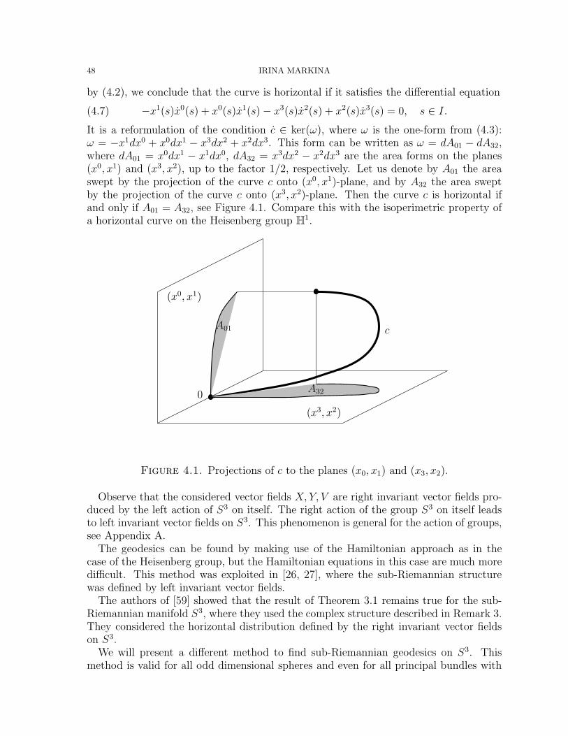
48 IRINA MARKINA
by (4.2), we conclude that the curve is horizontal if it satisfies the differential equation
(4.7) −x1(s)x0(s) + x0(s)x1(s)− x3(s)x2(s) + x2(s)x3(s) = 0, s ∈ I.
It is a reformulation of the condition c ∈ ker(ω), where ω is the one-form from (4.3):ω = −x1dx0 + x0dx1 − x3dx2 + x2dx3. This form can be written as ω = dA01 − dA32,where dA01 = x0dx1 − x1dx0, dA32 = x3dx2 − x2dx3 are the area forms on the planes(x0, x1) and (x3, x2), up to the factor 1/2, respectively. Let us denote by A01 the areaswept by the projection of the curve c onto (x0, x1)-plane, and by A32 the area sweptby the projection of the curve c onto (x3, x2)-plane. Then the curve c is horizontal ifand only if A01 = A32, see Figure 4.1. Compare this with the isoperimetric property ofa horizontal curve on the Heisenberg group H1.
0
(x0, x1)
(x3, x2)
cA01
A32
Figure 4.1. Projections of c to the planes (x0, x1) and (x3, x2).
Observe that the considered vector fields X, Y, V are right invariant vector fields pro-duced by the left action of S3 on itself. The right action of the group S3 on itself leadsto left invariant vector fields on S3. This phenomenon is general for the action of groups,see Appendix A.
The geodesics can be found by making use of the Hamiltonian approach as in thecase of the Heisenberg group, but the Hamiltonian equations in this case are much moredifficult. This method was exploited in [26, 27], where the sub-Riemannian structurewas defined by left invariant vector fields.
The authors of [59] showed that the result of Theorem 3.1 remains true for the sub-Riemannian manifold S3, where they used the complex structure described in Remark 3.They considered the horizontal distribution defined by the right invariant vector fieldson S3.
We will present a different method to find sub-Riemannian geodesics on S3. Thismethod is valid for all odd dimensional spheres and even for all principal bundles with
GEOMETRY WITH CONSTRAINTS 49
the appropriate choice of metrics. It will be one of the main points of consideration inSection 5.
4.2. Sub-Riemannian structures on S7.
4.2.1. Tangent vector fields for S7. In this section we obtain two structurally differenttypes of horizontal distributions on S7. One of them is of rank 6 and the other is of rank4. We start from the construction of a convenient basis of tangent vector fields to S7.
The multiplication of unit octonions is not associative, therefore S7 is not a groupin contrast with S3. Nevertheless, we are still able to use the multiplication law inorder to find global non-vanishing tangent vector fields. In calculations we use a slightlydifferent multiplication table of unit octonions from what we considered in Subsection 3.3and that leads to a different product. It is more convenient for our purpose in thissubsection. Both the multiplication table of unit octonions and the product of twoarbitrary octonions are presented in Appendix B.
The multiplication rule induces a matrix representation of the right octonion multi-plication, given explicitly by:
drτ =
y0 −y1 −y2 −y3 −y4 −y5 −y6 −y7
y1 y0 y3 −y2 y5 −y4 −y7 y6
y2 −y3 y0 y1 y6 y7 −y4 −y5
y3 y2 −y1 y0 y7 −y6 y5 −y4
y4 −y5 −y6 −y7 y0 y1 y2 y3
y5 y4 −y7 y6 −y1 y0 −y3 y2
y6 y7 y4 −y5 −y2 y3 y0 −y1
y7 −y6 y5 y4 −y3 −y2 y1 y0
.
for τ = y0 +∑7
k=1 ykjk.We are able to find globally defined tangent vector fields which are invariant under the
right multiplication rule. We proceed by analogy with constructions made for S3. Theexplicit formulas of vector fields are given in Appendix B. The vector fields Y1, . . . , Y7form a frame for TS7 and Y0 is the normal to S7. More explicitly(
Yi(τ), Yj(τ))τ
= δij , τ ∈ S7, i, j ∈ 0, 1, . . . , 7,where (·, ·) is the standard inner product in R8, and δij stands for Kronecker’s delta.
4.2.2. CR structure and the Hopf map on S2n+1. Before we go further in studying struc-tures on S7, we present general relations between the CR structures on odd dimensionalspheres and the higher dimensional Hopf fibration.
Consider S2n+1 = z ∈ Cn+1 | ‖z‖2 = 1. Then the right U(1)-action on S2n+1 givenby
(z0, . . . , zn).υ = (z0υ, . . . , znυ),
for υ ∈ U(1) and (z0, . . . , zn) ∈ S2n+1, induces the principal U(1)-bundle U(1) →S2n+1 h−→ CP n given explicitly by
S2n+1 $ (z0, . . . , zn) %→ h(z0, . . . , zn) = [z0 : · · · : zn] ∈ CP n,
50 IRINA MARKINA
where [z0 : · · · : zn] denotes homogeneous coordinates. This map is called higher Hopffibration. The kernel of the map h : S2n+1 → CP n gives the vertical space at each pointof S2n+1. The horizontal distribution or the Ehresmann connection D is given by theorthogonal complement to the vertical distribution V with respect to the inner product ofR2n+2. We show that the vertical space is always given by the action of standard almostcomplex structure on the normal vector field to S2n+1, and the Ehresmann connectioncoincides with the holomorphic tangent space at each point of S2n+1.
Theorem 4.1 asserts that any odd dimensional sphere has at least one globally definednon-vanishing tangent vector field. If the dimension of the sphere is of the form 4n + 1,then it has only one globally defined non-vanishing tangent vector field. If the dimensionof the sphere is of the form 4n+3, then the sphere admits at least three globally definednon-vanishing vector fields. Any sphere S2n+1 possesses the vector field
(4.8) V = −y1∂0 + y0∂1 − y3∂2 + . . .− y2n+2∂2n+1 + y2n+1∂2n+2.
Observe that this vector field has appeared already in two cases: as the vector field Vfor S3, and as the vector field Y1 for S7.
The vector field V encloses valuable information concerning the CR structure of S2n+1.A result of [13] states that the sphere S2n+1, as a smooth hypersurface in Cn+1, admitsa holomorphic tangent space of dimension dimR HqS
2n+1 = 2n for any point q ∈ S2n+1.The following lemma implies a description of the holomorphic tangent space HqS
2n+1 asthe orthogonal complement to V .
Lemma 1. Let W be an Euclidean space of dimension k+2, k ≥ 1, with the inner product(·, ·)W and let X, Y be two vectors from W . Consider an orthogonal decomposition W =
spanX, Y ⊕⊥ W with respect to (·, ·)W and an orthogonal endomorphism A : W →Wsuch that
A(spanX, Y ) = spanX, Y ,then W is an invariant space under the action of A, i.e.
A(W ) = W .
Proof. Let v ∈ W , then for any α, β ∈ R it is clear that(Av,αX + βY
)W
=(v, Atr(αX + βY )
)W
=(v, A−1(αX + βY )
)W
.
Since A(spanX, Y ) = spanX, Y , there exist a, b ∈ R such that
A−1(αX + βY ) = aX + bY,
and therefore,(Av,αX +βY
)W
=(v, aX + bY
)W
= 0, which implies that Av ∈ W . !As an application of Lemma 1, it is possible to obtain an explicit characterization of
the space HqS2n+1.
Lemma 2. The vector space HqS2n+1 is the orthogonal complement to the vector Vq ∈
TqS2n+1 from (4.8) for any q ∈ S2n+1.
Proof. Consider the vector space
Wq = spanN(q)⊕⊥ TqS2n+1 ∼= TqR2n+2,
GEOMETRY WITH CONSTRAINTS 51
where N(q) is the normal vector to S2n+1 at the point q. The standard almost complexstructure map J : Wq → Wq is orthogonal. Moreover, J(V (q)) = −N(q), J(N(q)) =
V (q). Using the decomposition Wq = Wq ⊕⊥ spanV (q), N(q), it is possible to apply
Lemma 1 in order to conclude that Wq, which is the orthogonal complement to V (q) in
TqS2n+1, is invariant under J . Since dimR Wq = 2n, we conclude that Wq = HqS
2n+1. !
The space HS2n+1 can also be described as the kernel of the one-form
θ = z0dz0 + . . . + zndzn.
Indeed, consider X ∈ HS2n+1. Then by straightforward calculations we have
(4.9) θ(X) = (X, N) + i(X, V ) = 0.
Lemma 2 provides a horizontal distribution of rank 2n for the spheres S2n+1, byconsidering the holomorphic tangent bundle: D = HS2n+1. The bracket generatingproperty follows from the following general result for an arbitrary contact manifold.
Definition 19. Let M be a (2n + 1)-dimensional manifold. A smooth one form ω iscalled contact if it satisfies the condition
ωq ∧ (dωq)n .= 0 for any q ∈ M.
The pair (M,ω) is called a contact manifold.
Lemma 3. Let M be a (2n+1)-dimensional contact manifold with contact form ω, thenD = ker(ω) is a bracket generating distribution of rank 2n and step 2.
Proof. Recall Cartan’s formula for a differential one-form ω, namely
(4.10) dω(X, Y ) = X(ω(Y ))− Y (ω(X))− ω([X, Y ]),
for all X, Y ∈ TM . It follows from (4.10) that D is Frobenius integrable if and only ifdω(X, Y ) = 0 for all X, Y ∈ D. Thus, if ω is a contact form, then dω(X, Y ) .= 0 forall X, Y ∈ TM and, therefore D is not integrable. This implies the bracket generatingproperty for D, since if [X, Y ]q /∈ Dq at any point q ∈ M for some Xq, Yq ∈ Dq thenspan[X, Y ]q⊕Dq = TqM . !
By Lemma 3, in order to prove that HS2n+1 is bracket generating, it is sufficient tofind a contact one-form ω such that HS2n+1 = ker(ω). To achieve this, let us consider
(4.11) ω = Im θ = −y1dy0 + y0dy1 − . . .− y2n+1dy2n + y2ndy2n+1
defined on S2n+1. By (4.9), the relation HS2n+1 = ker(ω) holds immediately.
Theorem 4.2. [47] The one-form ω defined in (4.11) is a contact form. More specif-ically, ω satisfies (dω)n ∧ ω = n! · 2ndvolS2n+1, where dvolS2n+1 is the volume form forS2n+1.
The following corollary holds by Lemma 3 and Theorem 4.2.
Corollary 1. The holomorphic tangent bundle HS2n+1 is a bracket generating distribu-tion of step 2 and rank 2n.
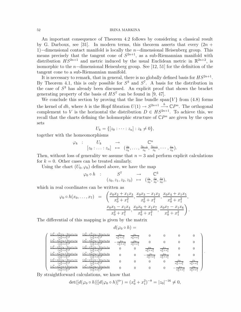
52 IRINA MARKINA
An important consequence of Theorem 4.2 follows by considering a classical resultby G. Darboux, see [31]. In modern terms, this theorem asserts that every (2n +1)−dimensional contact manifold is locally the n−dimensional Heisenberg group. Thismeans precisely that the tangent cone of S2n+1, as a sub-Riemannian manifold withdistribution HS2n+1 and metric induced by the usual Euclidean metric in R2n+2, isisomorphic to the n−dimensional Heisenberg group. See [12, 51] for the definition of thetangent cone to a sub-Riemannian manifold.
It is necessary to remark, that in general, there is no globally defined basis for HS2n+1.By Theorem 4.1, this is only possible for S3 and S7. A basis for the distribution inthe case of S3 has already been discussed. An explicit proof that shows the bracketgenerating property of the basis of HS7 can be found in [9, 47].
We conclude this section by proving that the line bundle spanV from (4.8) forms
the kernel of dh, where h is the Hopf fibration U(1) → S2n+1 h−→ CP n. The orthogonalcomplement to V is the horizontal the distribution D ∈ HS2n+1. To achieve this, werecall that the charts defining the holomorphic structure of CP n are given by the opensets
Uk = [z0 : · · · : zn] : zk .= 0,together with the homeomorphisms
ϕk : Uk → Cn
[z0 : . . . : zn] %→ ( z0
zk, . . . , zk−1
zk, zk+1
zk, · · · , zn
zk).
Then, without loss of generality we assume that n = 3 and perform explicit calculationsfor k = 0. Other cases can be treated similarly.
Using the chart (U0,ϕ0) defined above, we have the map
ϕ0 h : S7 → C3
(z0, z1, z2, z3) %→ ( z1
z0, z2
z0, z3
z0),
which in real coordinates can be written as
ϕ0 h(x0, . . . , x7) =
(x0x2 + x1x3
x20 + x2
1
,x0x3 − x1x2
x20 + x2
1
,x0x4 + x1x5
x20 + x2
1
,
x0x5 − x1x4
x20 + x2
1
,x0x6 + x1x7
x20 + x2
1
,x0x7 − x1x6
x20 + x2
1
).
The differential of this mapping is given by the matrix
d(ϕ0 h) =
(x21−x2
0)x2−2x0x1x3(x2
0+x21)2
(x20−x2
1)x3−2x0x1x2(x2
0+x21)2
x0x20+x2
1
x1x20+x2
10 0 0 0
(x21−x2
0)x3+2x0x1x2(x2
0+x21)2
(x21−x2
0)x2−2x0x1x3(x2
0+x21)2
− x1x20+x2
1
x0x20+x2
10 0 0 0
(x21−x2
0)x4−2x0x1x5(x2
0+x21)2
(x20−x2
1)x5−2x0x1x4(x2
0+x21)2
0 0 x0x20+x2
1
x1x20+x2
10 0
(x21−x2
0)x5+2x0x1x4(x2
0+x21)2
(x21−x2
0)x4−2x0x1x5(x2
0+x21)2
0 0 − x1x20+x2
1
x0x20+x2
10 0
(x21−x2
0)x6−2x0x1x7(x2
0+x21)2
(x20−x2
1)x7−2x0x1x6(x2
0+x21)2
0 0 0 0 x0x20+x2
1
x1x20+x2
1(x2
1−x20)x7+2x0x1x6(x2
0+x21)2
(x21−x2
0)x6−2x0x1x7(x2
0+x21)2
0 0 0 0 − x1x20+x2
1
x0x20+x2
1
.
By straightforward calculations, we know that
det([d(ϕ0 h)][d(ϕ0 h)]tr) = (x20 + x2
1)−8 = |z0|−16 .= 0,
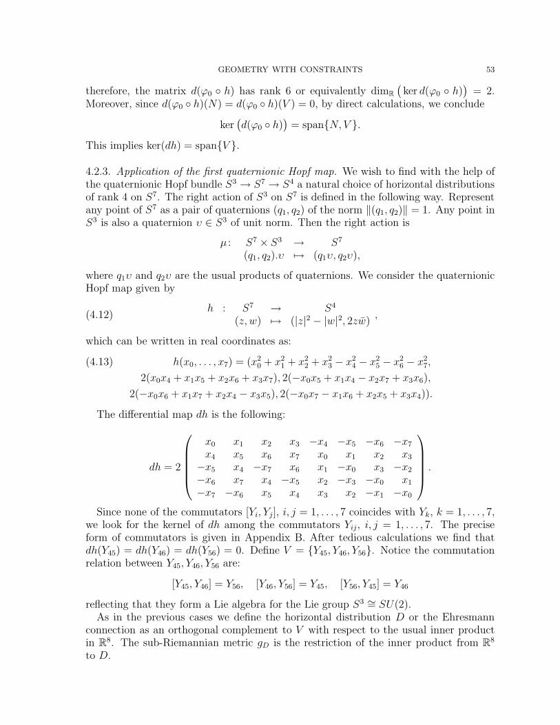
GEOMETRY WITH CONSTRAINTS 53
therefore, the matrix d(ϕ0 h) has rank 6 or equivalently dimR(ker d(ϕ0 h)
)= 2.
Moreover, since d(ϕ0 h)(N) = d(ϕ0 h)(V ) = 0, by direct calculations, we conclude
ker(d(ϕ0 h)
)= spanN, V .
This implies ker(dh) = spanV .
4.2.3. Application of the first quaternionic Hopf map. We wish to find with the help ofthe quaternionic Hopf bundle S3 → S7 → S4 a natural choice of horizontal distributionsof rank 4 on S7. The right action of S3 on S7 is defined in the following way. Representany point of S7 as a pair of quaternions (q1, q2) of the norm ‖(q1, q2)‖ = 1. Any point inS3 is also a quaternion υ ∈ S3 of unit norm. Then the right action is
µ : S7 × S3 → S7
(q1, q2).υ %→ (q1υ, q2υ),
where q1υ and q2υ are the usual products of quaternions. We consider the quaternionicHopf map given by
(4.12)h : S7 → S4
(z, w) %→ (|z|2 − |w|2, 2zw),
which can be written in real coordinates as:
h(x0, . . . , x7) = (x20 + x2
1 + x22 + x2
3 − x24 − x2
5 − x26 − x2
7,(4.13)
2(x0x4 + x1x5 + x2x6 + x3x7), 2(−x0x5 + x1x4 − x2x7 + x3x6),
2(−x0x6 + x1x7 + x2x4 − x3x5), 2(−x0x7 − x1x6 + x2x5 + x3x4)).
The differential map dh is the following:
dh = 2
x0 x1 x2 x3 −x4 −x5 −x6 −x7
x4 x5 x6 x7 x0 x1 x2 x3
−x5 x4 −x7 x6 x1 −x0 x3 −x2
−x6 x7 x4 −x5 x2 −x3 −x0 x1
−x7 −x6 x5 x4 x3 x2 −x1 −x0
.
Since none of the commutators [Yi, Yj], i, j = 1, . . . , 7 coincides with Yk, k = 1, . . . , 7,we look for the kernel of dh among the commutators Yij, i, j = 1, . . . , 7. The preciseform of commutators is given in Appendix B. After tedious calculations we find thatdh(Y45) = dh(Y46) = dh(Y56) = 0. Define V = Y45, Y46, Y56. Notice the commutationrelation between Y45, Y46, Y56 are:
[Y45, Y46] = Y56, [Y46, Y56] = Y45, [Y56, Y45] = Y46
reflecting that they form a Lie algebra for the Lie group S3 ∼= SU(2).As in the previous cases we define the horizontal distribution D or the Ehresmann
connection as an orthogonal complement to V with respect to the usual inner productin R8. The sub-Riemannian metric gD is the restriction of the inner product from R8
to D.
54 IRINA MARKINA
Remark 4. Another way to construct the horizontal distribution was proposed in [47]The authors presented several bracket generating distributions transversal to V . None ofthem has a globally defined non-vanishing basis, meanwhile the vertical space V has suchkind of the basis. The authors of the paper [9] presented another horizontal distributionof rank 4 that was constructed considering the Clifford algebra structure of S7 and thatpossesses a globally defined non-vanishing basis. However, in this case a globally definedbasis of the vertical space, different from V constructed above, was not found.
5. Principal bundles
In this section we show the explicit formulas for geodesics on any odd dimensionalspheres. They were found by making use of a result from [94]. To present this result wegive all necessary definitions, prove the theorem of existence of geodesics and apply itto odd dimensional spheres. At the end, we will give some applications of the geometryof principal bundles to physics and will illustrate them by exploiting the results fromprevious sections.
5.1. Ehresmann connection. In this subsection we will describe two possible waysto introduce sub-Riemannian structures on a smooth manifold M , provided that thereexists a submersion π : M → B to another smooth manifold B. We call the mapπ projection and the manifold B the base space. For q ∈ M we call the pre-imageFb = π−1(b), b = π(q), the fiber through a point q ∈ M . The set Fb is a smoothsubmanifold of M . Since the differential map dqπ is surjective for all q ∈ M , thekernel ker(dqπ) is non-empty. We denote it by Vq and call the vertical space at q ∈ M .The collection of all vertical space is called vertical distribution or vertical sub-bundleV ⊂ TM . The vertical space is actually the tangent space Vq = TqF to the fiber Fpassing through q.
Definition 20. An Ehresmann connection for a submersion π : M → B is a distributionD ⊂ TM that is everywhere transverse and of complementary dimension to the verticaldistribution V :
TqM = Dq ⊕ Vq. q ∈ M.
Notice that ⊕ denotes only transversality of two vector spaces at q ∈ M , but notorthogonality, because there was no any kind of metric defined on M up to the moment.The vector space Dp is an example of a horizontal vector space and the Ehresmannconnection is an example of a horizontal distribution. Notice that given a submersionwe always have a vertical distribution and the construction of the horizontal distributionor the Ehresmann connection is the question of mathematical art.
There are two ways to introduce the sub-Riemannian structure on a manifold M .
Case 1. Sub-Riemannian structure by restriction. Suppose that we havea submersion π : M → B and that the manifold M is endowed with a Riemannianmetric gM . Let Vq = ker(dqπ). Define the horizontal vector space Dq as the orthogonalcomplement to the vertical space Vq at each q ∈ M with respect to the given metricgM : Dq ⊕⊥ Vq = TqM . The obtained horizontal distribution D will be the Ehresmannconnection, since it is orthogonally transversal to V at each point. If we denote by gMD
the restriction of the Riemannian metric gM to the distribution D, then (M, D, gMD) is
GEOMETRY WITH CONSTRAINTS 55
the sub-Riemannian manifold defined by submersion π and the Riemannianmetric gM on M . In this case the sub-Riemannian length of a horizontal curve is equalto the Riemannian length, since the vertical components vanish.
Case 2. Induced sub-Riemannian structure. Suppose now that for the sub-mersion π : M → B the Ehresmann connection is defined, and moreover, the base man-ifold B is endowed with a Riemannian metric gB. Since the restriction dqπ|Dq : Dq →Tπ(q)B is an isomorphism, we can pullback the metric gB to the horizontal space Dq ateach q ∈ M . Denote the obtained metric by gBD
. Thus,
gBD(v, w) := gB(dqπ(v), dqπ(w)), v, w ∈ Dq, q ∈ M.
The obtained metric varies smoothly with q ∈ M . The triplet (M, D, gBD) is called a
sub-Riemannian manifold induced by the Ehresmann connection D on M andby the Riemannian metric gB on B. In this case we get the following properties.
1. If a horizontal curve γ is given on M , then the sub-Riemannian length of γ isequal to the Riemannian length of its projection to B. This is obvious, sincethe vertical component of the velocity vector of a horizontal curve γ in TqM isabsent, and moreover, the vertical space is projected to the 0-subspace in eachtangent space Tπ(q)B.
2. What happens if we are given a curve on the base space and we pull it back tothe manifold M? Define the horizontal lift of a curve c : I → B upto M . Thehorizontal lift of the curve c is a curve γ : I →M such that
(1) γ(t) ∈ Dγ(t) and (2) π(γ(t)) = c(t) for all t ∈ I.
The horizontal lift of a Riemannian geodesic in B is a sub-Riemannian geodesicin M . If the Riemannian geodesic in B is a length minimizers between its endpoints, then its horizontal lift is a sub-Riemannian length minimizer between thecorresponding fibers.
Remark 5. It is natural to ask, when the horizontal lift exists. We will not discussit here. But if it exists, then given a point q ∈ M and a curve c starting at π(q), thehorizontal lift γ of c starting from q ∈ M is unique.
Now, having these two ways of constructing sub-Riemannian structures on M , wecan ask when these structures coincide. Suppose we are given a submersion π of aRiemannian manifold (M, gM) to a Riemannian manifold (B, gB). If the restrictiondqπ|Dq : (Dq, dMD
) → (Tπ(q)B, gB) is a linear isometry for corresponding vector spacesfor all q ∈ M , then (M, D, gMD
) = (M, D, gBM). In this case the submersion π is actually
a Riemannian submersion, see Definition 41.
5.2. Metrics on principal bundles. A definition of a fiber bundle is given in AppendixA, Definition 58. We will present the definition of the principal bundle in the smoothsetting. Let M and B be smooth manifolds and let G be a Lie group that acts on theright on M . Recall that the action is by definition a smooth map.
Definition 21. Let M, B, and G be as above. A fiber bundle (F, M, B, π) is a smoothprincipal bundle if the typical fiber F has the structure of a Lie group G and, moreover,the group G acts freely and transitively (Definitions 55, 56) on each fiber.
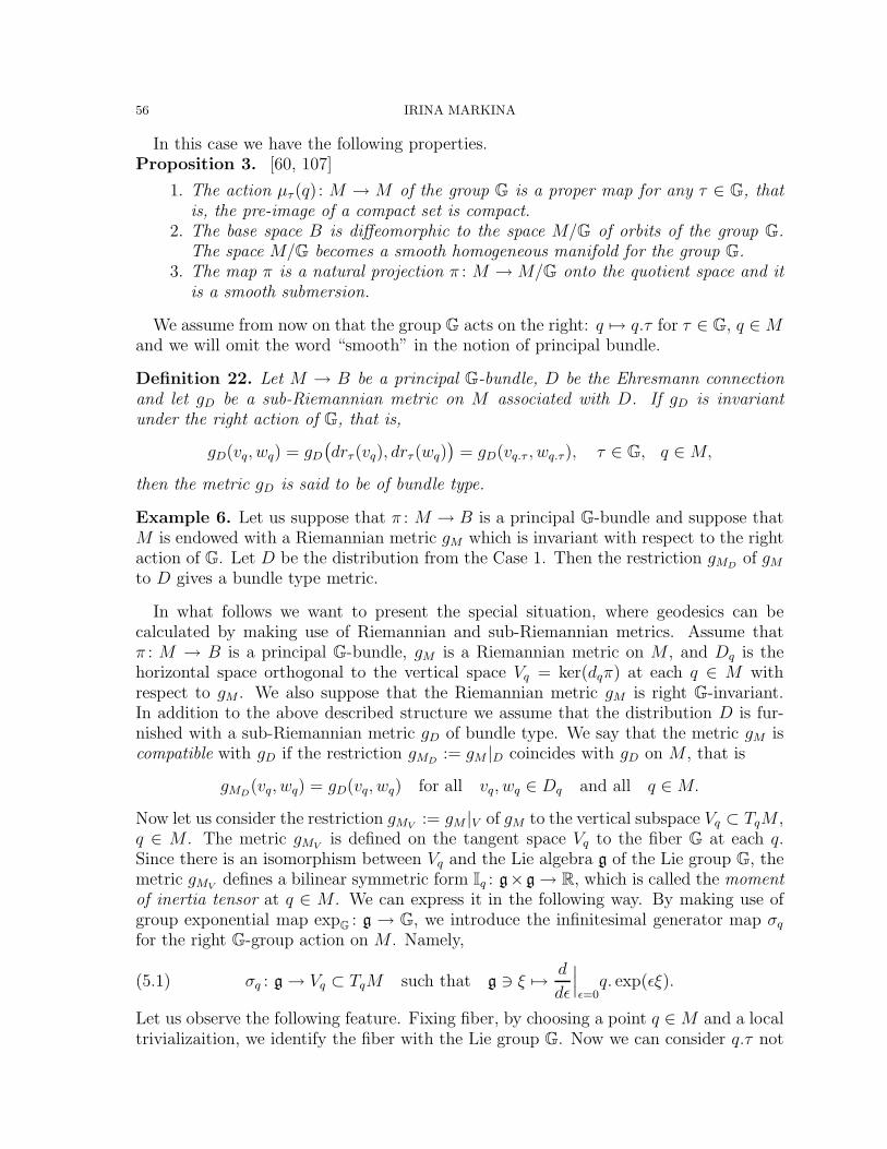
56 IRINA MARKINA
In this case we have the following properties.Proposition 3. [60, 107]
1. The action µτ (q) : M → M of the group G is a proper map for any τ ∈ G, thatis, the pre-image of a compact set is compact.
2. The base space B is diffeomorphic to the space M/G of orbits of the group G.The space M/G becomes a smooth homogeneous manifold for the group G.
3. The map π is a natural projection π : M → M/G onto the quotient space and itis a smooth submersion.
We assume from now on that the group G acts on the right: q %→ q.τ for τ ∈ G, q ∈ Mand we will omit the word “smooth” in the notion of principal bundle.
Definition 22. Let M → B be a principal G-bundle, D be the Ehresmann connectionand let gD be a sub-Riemannian metric on M associated with D. If gD is invariantunder the right action of G, that is,
gD(vq, wq) = gD
(drτ (vq), drτ (wq)
)= gD(vq.τ , wq.τ), τ ∈ G, q ∈ M,
then the metric gD is said to be of bundle type.
Example 6. Let us suppose that π : M → B is a principal G-bundle and suppose thatM is endowed with a Riemannian metric gM which is invariant with respect to the rightaction of G. Let D be the distribution from the Case 1. Then the restriction gMD
of gM
to D gives a bundle type metric.
In what follows we want to present the special situation, where geodesics can becalculated by making use of Riemannian and sub-Riemannian metrics. Assume thatπ : M → B is a principal G-bundle, gM is a Riemannian metric on M , and Dq is thehorizontal space orthogonal to the vertical space Vq = ker(dqπ) at each q ∈ M withrespect to gM . We also suppose that the Riemannian metric gM is right G-invariant.In addition to the above described structure we assume that the distribution D is fur-nished with a sub-Riemannian metric gD of bundle type. We say that the metric gM iscompatible with gD if the restriction gMD
:= gM |D coincides with gD on M , that is
gMD(vq, wq) = gD(vq, wq) for all vq, wq ∈ Dq and all q ∈ M.
Now let us consider the restriction gMV:= gM |V of gM to the vertical subspace Vq ⊂ TqM ,
q ∈ M . The metric gMVis defined on the tangent space Vq to the fiber G at each q.
Since there is an isomorphism between Vq and the Lie algebra g of the Lie group G, themetric gMV
defines a bilinear symmetric form Iq : g×g→ R, which is called the momentof inertia tensor at q ∈ M . We can express it in the following way. By making use ofgroup exponential map expG : g → G, we introduce the infinitesimal generator map σq
for the right G-group action on M . Namely,
(5.1) σq : g → Vq ⊂ TqM such that g $ ξ %→ d
dε
∣∣∣ε=0
q. exp(εξ).
Let us observe the following feature. Fixing fiber, by choosing a point q ∈ M and a localtrivializaition, we identify the fiber with the Lie group G. Now we can consider q.τ not
GEOMETRY WITH CONSTRAINTS 57
only as a right action of the Lie group G (τ ∈ G) on M along the fiber, but also as theaction on the left of q (considered as an element of G) on the Lie group G, or
(5.2) q.τ = lq(τ).
So, it is convenient to think of the infinitesimal generator of the right action as of alocally left invariant vector field, since
σq(ξ) =d
dε
∣∣∣ε=0
q. exp(εξ) =d
dε
∣∣∣ε=0
lq(exp(εξ)
)= dlq(ξ)
by the property 1 in Theorem 8.2 or by the definition of the exponential curve in Sub-section 3.1, see (3.1). Then we define the bilinear symmetric tensor Iq : g × g → Rby
(5.3) Iq(ξ, η) = gMV(σq(ξ), σq(η)), ξ, η ∈ g, q ∈ M.
We conclude that if a right G-invariant Riemannian metric gM is given on a principalG-bundle π : M → B, then we define the sub-Riemannian structure (D, gMD
), whereD = V ⊥ and the moment of inertia tensor Iq (5.3) by means of restrictions of gM .
Conversely, if we have a sub-Riemannian structure (D, gD) with the metric gD ofbundle type and a moment of inertia tensor Iq : g× g → R, q ∈ M , then we can definea Riemannian metric gM as follows. Let us write any vector vq ∈ TqM according to thetransversal decomposition Dq ⊕ Vq as vq = vDq + vVq . Then the Riemannian metric gM
is defined by
gM(vq, wq) := gD(vDq , wDq) + Iq
(σ−1
q (vVq), σ−1q (wVq)
),
where the inverse map σ−1q is well defined. In order to check that the obtained Riemann-
ian metric gM is compatible with the bundle type metric gD we observe that
• Dq and Vq become orthogonal with respect to gM , since if vq ∈ Dq and wq ∈ Vq,then g(vq, wq) = gD(vq, 0) + Iq
(0, σ−1
q (wq))
= 0;• the restriction of gM to the distribution D coincides with gD,• to be right G-invariant the metric gM has to satisfy the relation
(5.4) gM(vq, wq) = gM(drτ (vq), drτ(wq)) = gM(vq.τ , wq.τ).
Let us reformulate the last condition in terms of the symmetric bi-linear tensor Iq.The left-hand side of (5.4) yields
(5.5) gM(vq, wq) = gD(vDq , wDq) + Iq(ξ, η),
where σq(ξ) = vVq , and σq(η) = wVq . The right hand side of (5.4) leads to
(5.6) gM(vq.τ , wq.τ) = gD(drτ (vDq), drτ (wDq)) + Iq.τ
(ζ ,χ
),
where σq.τ (ζ) = drτσq(ξ) and σq.τ (χ) = drτσq(η). Let us calculate drτσq(ξ). Weget
drτσq(ξ) =d
dε
∣∣∣ε=0
q exp(εξ)τ =d
dε
∣∣∣ε=0
qτ(τ−1 exp(εξ)τ
)=
d
dε
∣∣∣ε=0
qτ exp(εAdτ−1(ξ)
)= σq.τ
(Adτ−1(ξ)
).(5.7)
58 IRINA MARKINA
where Ad is the adjoint action of G over g, for definition see Example 13. Forthe relation of the adjoint map and the exponential map see Appendix A. Anal-ogously, we get drτσq(η) = σq.τ
(Adτ−1(η)
). Since gD is right invariant by defini-
tion of bundle type metric, the equalities (5.4), (5.5), and (5.6) imply
Iq(ξ, η) = Iqτ
(Adτ−1(ξ), Adτ−1(η)
)or Iqτ (ξ, η) = Iq
(Adτ (ξ), Adτ (η)
)by changing q to qτ−1, and then, τ−1 to τ . We conclude that to make theconstructed Riemannian metric gM invariant under the right action of the Liegroup G, we have to require that the given inertia tensor Iq should be invariantwith respect of the adjoint action of G on its Lie algebra g.
After all these discussions, we define a metric that we will work with. We will use theterminology of [94].
Definition 23. A Riemannian metric gM on a smooth manifold M is said to be ofconstant bi-invariant type if
1. gM is right G invariant,2. its inertia tensor Iq is independent of q ∈ M .
The word “constant” refers to the independence of the moment of inertia tensor fromthe points of the manifold. The bi-invariance reflects the fact that the inertia tensordefines a bi-invariant metric along the fiber G. We discuss it in the following remark.
Remark 6. Bi-invariant metrics on Lie group. Since the Lie algebra g is relatedto tangents spaces TqG to its group by left translations, any tensor Θ on the algebra gcorresponds to a left invariant tensor T on its group G, because T is defined by makinguse of left translations to bring Θ to each point q ∈ G. If, moreover, the tensor Θ on g isinvariant under the adjoint action of G on its Lie algebra g, then the left invariant tensorT on G becomes right invariant. Applying this considerations to the bi-linear symmetricnon-degenerate form Iq on g, we obtain that it generates a bi-invariant metric on thefiber G through the point q. We see that the adjoint invariance on g means that Iq isconstant along the fiber through point q.
5.3. Geodesics theorem. Before we state and prove one of the principle theorems, weformulate an auxiliary statement.
Let G be a Lie group, g be its Lie algebra and let gG be a bi-invariant Riemannianmetric on the group, that may be given by an adjoint invariant bi-linear symmetric formon g as was noticed in Remark 6. Thus, the Lie group is also considered as a Riemannianmanifold (G, gG). There are two exponential maps defined in this case: the groupexponential expG : g → G and the Riemann exponential map (expR)e : TeG ∼ g → G.
Proposition 4. [89] In the above stated notations two exponential maps coincide.
In other words the Riemannian geodesic through the identity of the group G coincideswith the one-parameter subgroup produced by the group exponential map.
Let π : M → B be a principal G-bundle and let gM be a Riemannian metric of constantbi-invariant type. Let D be the Ehresmann connection which is orthogonal with respectto gM to the vertical space Vq at each q ∈ M . Let gD and gV denote restrictions of gM toD and V , respectively. Recall that the infinitesimal action σq : g → Vq is an isomorphism
GEOMETRY WITH CONSTRAINTS 59
by (5.1). Denote by projq the projection from TqM to Vq at each q ∈ M . The compositionA = σ−1
q projq is called the g-valued connection form, see diagram (5.8).
(5.8) gσq
∼=##ker(dqπ) = Vq
σ−1q
$$ TqM
A
%% proj.&& .
Let expR be the Riemannian exponential map generated by gM and let γv,R(t) =expR(tv) be the Riemannian geodesic passing through q ∈ M with the initial velocityvector v ∈ TqM . We project this Riemannian geodesic to the base manifold B obtaininga curve π(γv,R). Then we lift horizontally π(γv,R) to M and obtain a curve that wedenote by γsR.Theorem 5.1. [94] In the above notations the curve γsR is a normal sub-Riemanniangeodesic starting at q ∈ M . It is given by the formula
(5.9) γsR(t) = γv,R(t) expG(−tAq(v)), v ∈ TqM
Moreover all normal sub-Riemannian geodesics are given by the formula (5.9).
Proof. We follow the ideas in [94]. Since the decomposition of D ⊕⊥ V is orthogonalwith respect to the Riemannian metric gM , and gD and gV are defined by the restrictionof gM to the corresponding distributions, we can define three Hamiltonian functions HR,HsR and HV . Here we denote by HR the Riemannian Hamiltonian function related tothe Riemannian metric gM , by HsR the sub-Riemannian Hamiltonian function related tothe metric gD, see (2.12) and by HV the vertical Hamiltonian function related to gV andconstructed by the same rule as in (2.12). Then the orthogonality of the compositionD ⊕⊥ V implies that HsR = HR −HV . Let us also use the notations
expR : TqM →M, expsR : Dq →M, expV : Vq →M, q ∈ M.
The rough idea of the proof is to show that if these Hamiltonian functions Poissoncommute, then the corresponding flows on T ∗M produced by its Hamiltonian vectorfields also commute. Therefore, if v = vD + vV is the initial velocity vector writtenaccording to the decomposition Dq⊕⊥ Vq = TqM , then the flow commutativity propertyleads to the commutativity of the exponential maps, that is
expsR(tvD) = expR(tv) expV (−tvV ).
In the last step of the proof we observe that expV (−tvV ) coincides with the group Gexponential map because the metric gV is bi-invariant along the fiber through q ∈ M .
The first step in the proof of the theorem is to show that the Hamiltonian functionsHR, HsR, and HV Poisson commute. Actually we only need to show that HsR, HV = 0.We use the local trivialization for the bundle π : M → B. Let U ⊂ B be a neighborhoodof π(q), then π−1(U) is diffeomorphic to G × U . At the level of cotangent bundles itleads to the diffeomorphism
T ∗π−1(U)M = T ∗(G× U) ∼= T ∗G× T ∗U.
Let us use the coordinates π−1(U) $ q = (τ, b) = (τ 1, . . . τ l, b1, . . . , bk) ∈ G× U , l + k =n = dim M for points, and T ∗q M $ λ = (µ, p) = (µ1, . . . , µl, p1, . . . , pk) ∈ T ∗q G × T ∗b U
60 IRINA MARKINA
for momenta. Since the moment of inertia tensor I is independent of q ∈ M and it isindependent of the horizontal part of any vector, the dual tensor I∗ : g∗× g∗ → R is alsoindependent of q ∈ M and p ∈ T ∗b U . This implies that HV (τ, b, µ, p) is only a functionof the µ-variables: HV = HV (µ). The right invariant property of the metric gD leads toindependence of the corresponding Hamiltonian function HsR from τ -slot of variables:HsR = HsR(b, µ, p). The Poisson brackets are
HsR, HV =( l∑
j=1
∂HsR
∂µj
∂HV
∂τj+
k∑j=1
∂HsR
∂pj
∂HV
∂bj
)−( l∑
j=1
∂HsR
∂τj
∂HV
∂µj+
k∑j=1
∂HsR
∂bj
∂HV
∂pj
).
In the last sum we have ∂HV (µ)∂τj
= ∂HV (µ)∂bj
= ∂HV (µ)∂pj
= 0 and ∂HsR(b,µ,p)∂τj
= 0, that implies
HsR, HV = 0. We conclude that flows ΦR,ΦsR, and ΦV on T ∗M corresponding to−→HR,−→
H sR, and−→H V , respectively, commute. Recall that the exponential map is a composition
of the following maps, see (2.10).
(5.10) TqMι !!
exp
""TMduality
!! T ∗MΦ(q,λ)
!! T ∗Mpr∗M !! M,
where we have to change the corresponding flows and TqM to Dq and Vq respectively.We see that the commutation of the flows leads to the commutation of the exponentialmaps and we have
(5.11) expsR(tv) = expR(tv) expV (−tv), t ∈ I
for HsR = HR − HV , where v ∈ TqM is the initial velocity vector that corresponds tothe choice of λ in the flow. The curve expR(tv) = γv,R(t), t ∈ I, is the Riemanniangeodesic on M , starting from q ∈ M with the initial velocity v ∈ TqM . Recall, that theexponential curve expV (−tv) produced by the Hamiltonian function HV (µ) is indepen-dent of p variables in the momentum slot. It gives expV (−tv) = expV (−tvV ). Now weexploit the fact that the Riemannian geodesic expV (−tvV ) coincides with the geodesic(or one-parametric subgroup) given by the group exponential map expG(−tσ−1(vV )).The composition of the projection of v to the vertical space Vq and of the map σ−1
q iscalled a g-valued connection form Aq : TqM → g, see (5.8). So equation (5.11) takes theform (5.9).
Let us make some observations. The vector v is just an initial velocity vector at q ∈ M .The element −tAq(v) ∈ g, and therefore, the vector tv − σ(tAq(v)) is horizontal for anyt ∈ I. So the velocity vector of the resulting curve in the right-hand side of (5.11) ishorizontal for any moment t, and the resulting curve in the left hand side is a horizontalgeodesic. !
5.3.1. Geodesics on odd dimensional spheres. In the case of odd dimensional spheres
S2n+1 = (z0, z1, . . . , zn) ∈ Cn+1 |n∑
j=1
|zj|2 = 1,
there is a natural action of U(1) given by q.υ = (z0υ, z1υ, . . . , znυ), where υ ∈ U(1).This action induces the Hopf fibration U(1) → S2n+1 → CP n, which forms a principal
GEOMETRY WITH CONSTRAINTS 61
U(1)−bundle with connection D given by the orthogonal complement to the vector field
(5.12) Vq = −y0∂x0 + x0∂y0 − . . .− yn∂xn + xn∂yn
at each q = (x0, y0, . . . , xn, yn) ∈ S2n+1, zj = xj + iyjnj=0, with respect to the usual
inner product in R2n+2. As it was shown, this distribution can be also given by kerωwith respect to the contact form ω = −y0dx0 + x0dy0 − . . .− yndxn + xndyn. Note thatVq = qi, q ∈ S2n+1, where q is thought of as a radial vector at the origin to the unitesphere, i is the complex imaginary unit, and q.i = qi, i ∈ u(1) is the u(1) action.
Consider (S2n+1, D, gD) as a sub-Riemannian manifold with the sub-Riemannian met-ric gD obtained by the restriction of the usual Riemannian metric g on TS2n+1 to thedistribution D. As a direct application of Theorem 5.1, it is possible to describe allnormal sub-Riemannian geodesics for S2n+1. The Lie algebra u(1) is one dimensional,its typical elements are purely imaginary numbers: ξ = iα. The u(1)−valued connectionform is Aq(v) = ig(v, Vq), v ∈ TqS
2n+1 and g(v, Vq) is just the projection of v to thevertical space Vq by making use of the Riemannian metric g. The Riemannian metric gon S2n+1 is of constant bi-invariant type, because we have
σq(ξ) =d
dε
∣∣∣∣ε=0
q expu(1)(εξ) = q.iα = αVq,
for any q ∈ S2n+1 and ξ = iα ∈ u(1). Therefore, the moment of inertia tensor is givenby
Iq(ξ, ξ) = Iq(iα, iα) = g(αVq, αVq) = αα,
which does not depend on q ∈ M . By Theorem 5.1, we have the following result.
Proposition 5. Let q ∈ S2n+1 and v ∈ TqS2n+1. If γR(t) = (z0(t), . . . , zn(t)) is the
great circle satisfying γR(0) = q and γR(0) = v, then the corresponding sub-Riemanniangeodesic γsR is given by
(5.13) γsR(t) =(z0(t)e
−itg(v,Vq), . . . , zn(t)e−itg(v,Vq)), t ∈ R.
To analyze formula (5.13) we recall that the Riemannian geodesic starting at q ∈ Sn
with a velocity v ∈ TqSn for any sphere Sn is a submanifold of Rn+1 given by:
(5.14) γR(t) = q cos(‖v‖t) +v
‖v‖ sin(‖v‖t), where ‖v‖ =√
g(v, v).
The great circle γR(t) on S2n+1, considered as a submanifold of R2(n+1) ∼= Cn+1, will bewritten in complex notation as γR(t) = (z0(t), . . . , zn(t)). Observe that V (γ(t)) = γ(t).iand Vq = V (γ(0)).
The following corollary can be thought of as a sort of Pythagoras theorem for sub-Riemannian spheres.
Corollary 2. For a horizontal sub-Riemannian geodesic on S2n+1 of the form (5.13)the following equation holds
‖γsR(t)‖2 + g2(v, Vq) = ‖v‖2.
Thus, its sub-Riemannian velocity is constant and its sub-Riemannian length for t ∈ [a, b]
is 9(γ) = (b− a)√‖v‖2 − g(v, Vq)2.
62 IRINA MARKINA
Proof. Denote by (·, ·)H the standard Hermitian product in Cn+1, Re (·, ·)H = g(·, ·). Bystraightforward calculations, we have
(γsR, γsR)H =((−ig(v, Vq)γR + γR)e−itg(v,Vq), (−ig(v, Vq)γR + γR)e−itg(v,Vq)
)H
= g(v, Vq)2(γR, γR)H + (γR, γR)H + g(v, Vq)
(i(γR, γR)H − i(γR, γR)H
)= g(v, Vq)
2 + ‖v‖2 − 2g(v, Vq)2.
The assertion follows. !
Corollary 3. If a curve γsR(t) = γR(t)e−itg(v,Vq) is parameterized by arc length then‖v‖2 = 1 + g(v, Vq)
2.
Corollary 4. The set of sub-Riemannian geodesics arising from the great circles γR(t),such that γR(0) ∈ D is diffeomorphic to CP n.
Proof. In this case, any sub-Riemannian geodesic starting at q ∈ S2n+1 with the initialvelocity v ∈ D ⊂ TqS
2n+1 coincides with the corresponding great circle, because the con-dition γR(0) ∈ D is equivalent to g(v, Vq) = 0, thus γsR(t) = p cos(‖v‖t) + v
‖v‖ sin(‖v‖t),whose loci is uniquely determined by the point [v] ∈ CP n. !
Observe that the manifold CP n can be seen as a submanifold of S2n+1 which istransversal to V along the fiber containing q and it can be thought of as a sophis-ticated analogue of the horizontal space at the identity in the (2n + 1)−dimensionalHeisenberg group.
5.3.2. Curvature or charge of sub-Riemannian geodesics on S3. The following equation
(5.15) ∇γsRγsR + 2κJ(γsR) = 0,
obtained by variational method, is true for the geodesics in S3 [59]. Here ∇ is theLevi-Civita connection associated with the Riemannian metric on S3 and J is an almostcomplex structure on S3 satisfying J(X) = −Y , J(Y ) = X .
The geometers call the parameter κ in (5.15) the curvature of γsR, since after pro-jecting the curve γsR via the Hopf fibration, κ becomes precisely the curvature of theprojected curve in S2. Note that curves of zero curvature are the horizontal great circles.Physicists call the parameter κ charge and denote it by λ. We return to the notion of acharge later in Subsection 5.5. We wish to find a relation between two different equationsfor geodesics (5.15) and (5.9).
Proposition 6. The curvature of the sub-Riemannian geodesic γsR(t) = γR(t)e−itg(v,Vq)
in S3, starting from q ∈ S3 with an initial velocity v ∈ TqS3, parameterized by arc length,
equals the value g(v, Vq).
Proof. Recall that the Lie group structure of S3 as of the set of unit quaternions, inducesthe globally defined vector fields (4.2). Let q = (x0, x1, x2, x3) = γ(0) ∈ S3 be the initialpoint of γ and let v = (v0, v1, v2, v3) = γR(0) ∈ TqS
3 be the initial velocity of thecorresponding great circle γR. By direct calculation, we have
(5.16) γ(t) = fX(t)X(γ(t)) + fY (t)Y (γ(t)),
GEOMETRY WITH CONSTRAINTS 63
where, denoting α = g(v, X), β = g(v, Y ), we have
fX(t) = α cos(2tg(v, V )) + β sin(2tg(v, V )),
fY (t) = β cos(2tg(v, V ))− α sin(2tg(v, V )).
It follows from this decomposition that
(5.17) J(γ(t)) = −fY (t)X(γ(t)) + fX(t)Y (γ(t)).
It remains to determine the term ∇γ γ. As it is well-known for submanifolds of Rn, thevector field ∇γ γ corresponds to the projection of the second derivative γ to the tangentspace of the submanifold. In this case, differentiating (5.16) we obtain
∇γ γ = 2g(v, V )(fY (t)X(γ(t))− fX(t)Y (γ(t))) = −2g(v, V ) J(γ(t)).
This finishes the proof. !
In [59] the problem of existence of closed sub-Riemannian geodesics is also discussed.Their result states that a complete geodesic γ in S3 parameterized by arc length, withcurvature κ is closed, if and only if, κ/
√1 + κ2 ∈ Q. This result can be generalized to
any odd dimensional sphere.
Proposition 7. Let γsR : R → S2n+1 be a complete sub-Riemannian geodesic parame-terized by arc length, with an initial velocity v ∈ TqS
2n+1. Then γsR is closed if andonly if
g(v, Vq)√1 + g2(v, Vq)
∈ Q.
Proof. The curve γsR : R → S2n+1 is closed, if and only if,
q = e−iT g(v,Vq)
(q cos(‖v‖T ) +
v
‖v‖ sin(‖v‖T )
)for some T > 0. Since v ∈ TqS
2n+1, we know that v is orthogonal to the vector joining0 ∈ R2n+2 and q, with respect to g. Thus, sin(‖v‖T ) = 0, which forces T = kπ/‖v‖,k ∈ Z. To complete the argument, we only need to see that ±e−iπk
(g(v,Vq)
‖v‖)q = q, if and
only if,
g(v, Vq)
‖v‖ =g(v, Vq)√
1 + g2(v, Vq)∈ Q,
where we have used Corollary 3. !
Exercise.
1. Calculate directly that the curve (5.9) is horizontal.2. Write the equation of geodesics starting from the point q = (1, 0, 0, 0). What is
the value of κ at q = (1, 0, 0, 0)?
64 IRINA MARKINA
5.3.3. Sub-Riemannian geodesics on S4n+3. Let us consider the sphere
S4n+3 = (q0, . . . , qn) ∈ Qn+1 |n∑
j=0
|qj|2 = 1.
The right action of Sp(1) ∼= SU(2) ∼= S3 on S4n+3 is defined by q.υ = (q0, . . . , qn).υ =(q0υ, . . . , qnυ), q ∈ S4n+3. This action induces a quaternionic Hopf fibration S3 →S4n+3 → HP n, given by
(5.18)h : S4n+3 → HP n
(q0, . . . , qn) %→ [q0 : . . . : qn].
This map forms a principal S3−bundle with the Ehresmann connection given by theorthogonal complement to the vector fields
V 1q = −y0∂x0 + x0∂y0 + w0∂z0 − z0∂w0 − . . .− yn∂xn + xn∂yn + wn∂zn − zn∂wn,
V 2q = −z0∂x0 − w0∂y0 + x0∂z0 + y0∂w0 − . . .− zn∂xn − wn∂yn + xn∂zn + yn∂wn,
V 3q = −w0∂x0 + z0∂y0 − y0∂z0 + x0∂w0 − . . .− wn∂xn − zn∂yn + yn∂zn + xn∂wn,
at each q = (x0, y0, z0, w0 . . . , xn, yn, zn, wn) ∈ S4n+3, with respect to the usual Riemann-ian metric g on S4n+3. It is easy to see that the following commutation relations holdfor V 1, V 2, V 3
[V 1, V 2] = V 3, [V 2, V 3] = V 1, [V 3, V 1] = V 2.
Thus one recovers the fact that spanV 1q , V 2
q , V 3q considered as the Lie algebra sp(1) is
isomorphic to the Lie algebra of the Lie group S3.All in all, the studied sub-Riemannian manifold is (S4n+3, D, gD), where D ⊕⊥ V =
spanV 1, V 2, V 3 with respect to the usual metric g in TS4n+3 and gD is the restrictionof g to D. Compare it with the sub-Riemannian manifold S2n+1.
It is an established fact that the distribution D is bracket generating. The geometryof spheres S4n+3 is known to be a quaternionic analogue of CR-geometry, see [5]. Notethat the vectors V 1
q , V 2q , V 3
q coincide with q.i1, q.i2, q.i3, respectively. Here q.ik is theaction of sp(1).
To apply Theorem 5.1 in this situation, it is necessary to specify the sp(1)−valuedconnection form associated to the Hopf map h from (5.18). In this case, the connectionform is given by
A(v) = i1g(v, V 1q ) + i2g(v, V 2
q ) + i3g(v, V 3q ),
where v ∈ TqS4n+3. The Riemannian metric g is of constant bi-invariant type, since for
any q ∈ S4n+3 and ξ = i1α1 + i2α2 + i3α3 ∈ sp(1), αk ∈ R, k = 1, 2, 3, (ξ is a pureimaginary quaternion) we have
σq(ξ) =d
dε
∣∣∣∣ε=0
q expsp(1)(εξ) = α1q.i1 + α2q.i2 + α3q.i3 = α1V1q + α2V
2q + α3V
3q .
Therefore, the moment of inertia tensor, given by
Iq(ξ, ξ) = Iq
( 3∑k=1
ikαk,
3∑k=1
ikαk
)= g
( 3∑k=1
αkVkq ,
3∑k=1
αkVkq
)=
3∑k=1
αkαk,
does not depend on the point. As for Corollary 5, we have the following result.
GEOMETRY WITH CONSTRAINTS 65
Proposition 8. If γR(t) = (q0(t), . . . , qn(t)) is the great circle satisfying γR(0) = q andγR(0) = v ∈ TqS
4n+3, then the corresponding sub-Riemannian geodesic is given by
(5.19) γsR(t) =(q0(t) · e−tA(v), . . . , qn(t) · e−tA(v)
).
In Proposition 8, the quaternionic exponential is defined by
eai1+bi2+ci3 = cos√
a2 + b2 + c2 + sin√
a2 + b2 + c2 · ai1 + bi2 + ci3√a2 + b2 + c2
,
for a, b, c ∈ R. Note that the curve e−tA(v) is simply the Riemannian geodesic in S3
starting at the identity of the group e = (1, 0, 0, 0) ∈ S3, with initial velocity vector(0,−g(v, V 1
q ),−g(v, V 2q ),−g(v, V 3
q )).
Corollary 5. The set of sub-Riemannian geodesics in S4n+3 arising from great circlesγR(t), such that γR(0) is orthogonal to spanV 1
q , V 2q , V 3
q is diffeomorphic to HP n.
Corollary 6. Let γsR : R → S4n+3 be a complete sub-Riemannian geodesic parameterizedby arc length, with the initial velocity v ∈ TqS
4n+3. Then γ is closed if and only if
g(v, V 1q )
‖v‖2,g(v, V 2
q )
‖v‖2,g(v, V 3
q )
‖v‖2∈ Q.
Corollary 7. For the horizontal sub-Riemannian geodesic of the form (5.19) the equality‖γ(t)‖2 + ‖A(v)‖2 = ‖v‖2 holds, where ‖A(v)‖2 = g2(v, V 1
q ) + g2(v, V 2q ) + g2(v, V 3
q ).
We leave the proofs of Corollaries 5 - 7 as an exercise.
5.4. Geodesics related to Yang-Mills fields. This subsection is aimed at a descrip-tion of sub-Riemannian geodesics produced by a principal G-bundle π : M → B as wasdescribed in the Case 2 of Subsection 5.1. Recall that in this case the Ehresmann connec-tion or the horizontal distribution D transversal to the vertical distribution V = ker(dπ)is given. Moreover, the sub-Riemannian metric gD is given as a pullback of the Riemann-ian metric gB from TB to the distribution D. We also require that the sub-Riemannianstructure (D, gD) is invariant under the right action of the structure group G. We wantto write geodesic equations for the sub-Riemannian manifold (M, D, gD).
To describe sub-Riemannian geodesics and explain their physical meaning, we needto introduce more definitions related to the notion of a principal bundle. Let the basespace B be endowed with a Riemannian metric gB. A Riemannian metric is a positivelydefinite quadratic form and in physics it represents the kinetic energy of a system inthe space B. Consider electromagnetic charged particles (or color-charged particle, orparticle with other characteristics) moving in B under influence of some forces. Themotion of the particle is not free since it must respect some constraints. Let us avoidconstraints as we did solving the Dido problem. We add more variables that allowsto inherit the information about forces. In the enlarged space M we assume that thestructure group G acts freely and transitively such that M receives the structure ofprincipal G-bundle.
The motion on the total space M is governed by a Lagrangian. If the Lagrangianhas redundant degrees of freedom or gauges, then the transformations between possiblegauges, given by observed physical laws, are called gauge transformations, or gauge
66 IRINA MARKINA
symmetries. So gauge transformations are automorphisms of the principal bundle, andthey form a group with respect to the composition of the bundle automorphisms. Fixb ∈ B, then automorphisms αb of each fiber Fb of M form a copy of the group G. Alltogether they define the associated bundle A over B with the structure group G. Thegauge group Gau(M) consists of all smooth sections of the associated bundle A. Thetrivial section b → idb of the associated G-bundle corresponds to the identity bundleautomorphism, see [64, 91].
The electromagnetic charged particles are described by the theory of principal U(1)-bundles. We can think of charges as of elements of the space g∗ dual to the Lie algebra gcorresponding to one dimensional structure groups U(1) or R. In mathematical theorycharges are elements of dual Lie algebras, because they fit better to the situation inwhich the geodesics are produced by bi-characteristics on the co-tangent bundle T ∗Mof M . Yang and Mills proposed the theory generalizing the gauge theory from principalU(1)-bundles to principal U(n)-bundles. For instance, SU(2) symmetry group is usedin the isospin model, SU(2) × U(1) symmetry group describes electroweak interaction,and SU(3) symmetry group is the subject of quantum cromodynamics.
The G-group action on M , produces an action on T ∗M and both the Hamiltonianfunction and the flow on T ∗M corresponding to the Hamiltonian vector field are invariantunder this action. Thus, it seems natural to reduce the space T ∗M to the space of orbitsT ∗M/G and consider the flow on the reduced space T ∗M/G. This reduction is calledthe Poisson reduction. The idea to consider the reduction of spaces endowed with somestructures (Poisson, symplectic, Kahler) comes from works [84, 85]. The dynamics onthe reduced space is related to sub-Riemannian geodesics on M , whose projections onthe base space B are trajectories of the motion of charged particles in Yang - Mills fieldsand the corresponding equations are called the Wong equations.
In the case of a one dimensional structure group the dynamic is quite well known,since the reduced space T ∗M/G is diffeomorphic to T ∗B⊕R and for each fixed value ofthe charge we get its level set in T ∗M/G that is diffeomorphic to T ∗B. This level setsare glued together to form the entire reduced space T ∗M/G.
For a non-abelian group G acting on M the structure of the reduced space T ∗M/Gis more complicated and it is isomorphic to T ∗B ⊕ Ad∗(M), where we have to changethe quite simple component representing the abelian charge by R to the bundle Ad∗(M)over the same base space B that is associated with the principal G-bundle π : M → B.
The motion of a “free” particle on the base space B means absence of forces actingthere and the trajectory of “free motion” is the geodesic given by the equation
∇cc = 0, ∇ is the Levi-Civita connection on B.
If a force F is present, then the equation changes to the Newton equation
∇cc = F
of geodesics on the manifold B for a particle of constant charge and unit mass. If thecharge is non-abelian, then it is encoded in the bundle Ad∗(M) and the right hand sideof the last equation depends in a complicated way on charge. Moreover, the conditionon the level sets of an abelian charge changes to the requirement to be a “co-variantly
GEOMETRY WITH CONSTRAINTS 67
constant” charge. To formulate the Wong equation supplemented by the conservationcondition for the charge we start from necessary definitions.
5.4.1. Structure of the reduced space. Induced action of group on tangent andco-tangent bundles. Let π : M → B be a principle G-bundle. The right action ofG on M produces right actions on TM and T ∗M . They defined by the following:
(5.20)µ : TM ×G → TM
(q, v).τ %→ (q.τ, drτ (v)
),
and
(5.21)µ : T ∗M ×G → T ∗M
(q,ω).τ %→ (q.τ,(drτ )
∗(ω)),
where (drτ )∗ is the dual operator to the differential drτ of the right translation r by τ ∈ G.
The factorization of TM by the action (5.20) leads to the factor space TM/G withelements [q, v]. Define the projection π : TM/G → B by
π([q, v]) := π(q) ∈ B, [q, v] ∈ TM/G.
We get a vector bundle over the base space B, where we will denote the projection πsimple by π. Thus, we have π : TM/G → B. Analogously, taking the factor of T ∗M bythe action (5.21) of G, we get a vector bundle π : T ∗M/G → B.
We aim to construct the bundle map TM/G → TB. The principal G-bundle
π : M → B
after differentiating leads to the bundle map
dπ : TM → TB.
Let us take the factor by the action of G of both parts. The action of G over TB istrivial: TB/G = TB. Thus we get a bundle map
Wb
''
dqπ!! TbB
''
TM/G
((
prB
''
dπ !! TB
((
prB
''
B B.
By making use of the dual map (dπ)∗, we get an analogous bundle map
W ∗b
''
T ∗b B
''
(dqπ)∗&&
T ∗M/G
((
pr∗B''
T ∗B
((
pr∗B''
(dπ)∗&&
B B.
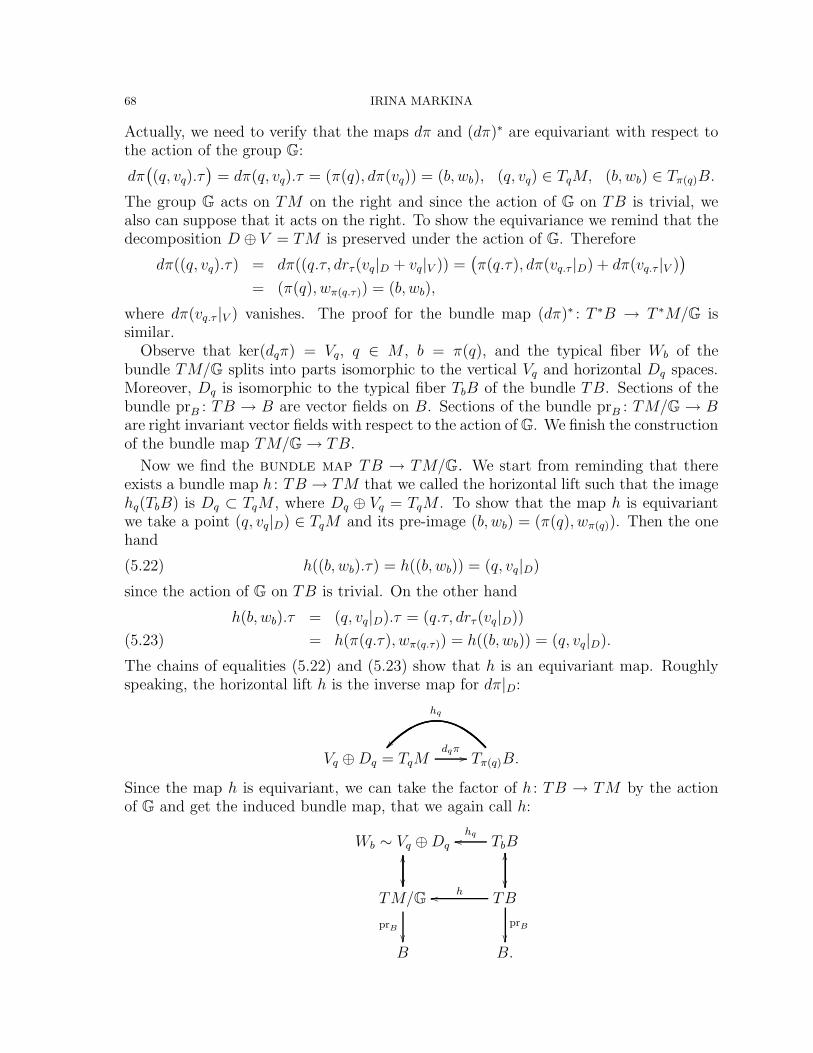
68 IRINA MARKINA
Actually, we need to verify that the maps dπ and (dπ)∗ are equivariant with respect tothe action of the group G:
dπ((q, vq).τ
)= dπ(q, vq).τ = (π(q), dπ(vq)) = (b, wb), (q, vq) ∈ TqM, (b, wb) ∈ Tπ(q)B.
The group G acts on TM on the right and since the action of G on TB is trivial, wealso can suppose that it acts on the right. To show the equivariance we remind that thedecomposition D ⊕ V = TM is preserved under the action of G. Therefore
dπ((q, vq).τ) = dπ((q.τ, drτ(vq|D + vq|V )) =(π(q.τ), dπ(vq.τ |D) + dπ(vq.τ |V )
)= (π(q), wπ(q.τ)) = (b, wb),
where dπ(vq.τ |V ) vanishes. The proof for the bundle map (dπ)∗ : T ∗B → T ∗M/G issimilar.
Observe that ker(dqπ) = Vq, q ∈ M , b = π(q), and the typical fiber Wb of thebundle TM/G splits into parts isomorphic to the vertical Vq and horizontal Dq spaces.Moreover, Dq is isomorphic to the typical fiber TbB of the bundle TB. Sections of thebundle prB : TB → B are vector fields on B. Sections of the bundle prB : TM/G → Bare right invariant vector fields with respect to the action of G. We finish the constructionof the bundle map TM/G → TB.
Now we find the bundle map TB → TM/G. We start from reminding that thereexists a bundle map h : TB → TM that we called the horizontal lift such that the imagehq(TbB) is Dq ⊂ TqM , where Dq ⊕ Vq = TqM . To show that the map h is equivariantwe take a point (q, vq|D) ∈ TqM and its pre-image (b, wb) = (π(q), wπ(q)). Then the onehand
(5.22) h((b, wb).τ) = h((b, wb)) = (q, vq|D)
since the action of G on TB is trivial. On the other hand
h(b, wb).τ = (q, vq|D).τ = (q.τ, drτ(vq|D))
= h(π(q.τ), wπ(q.τ)) = h((b, wb)) = (q, vq|D).(5.23)
The chains of equalities (5.22) and (5.23) show that h is an equivariant map. Roughlyspeaking, the horizontal lift h is the inverse map for dπ|D:
Vq ⊕Dq = TqMdqπ
!! Tπ(q)B.
hq
))
Since the map h is equivariant, we can take the factor of h : TB → TM by the actionof G and get the induced bundle map, that we again call h:
Wb ∼ Vq ⊕Dq
''
TbB
''
hq&&
TM/G
((
prB
''
TB
((
prB
''
h&&
B B.
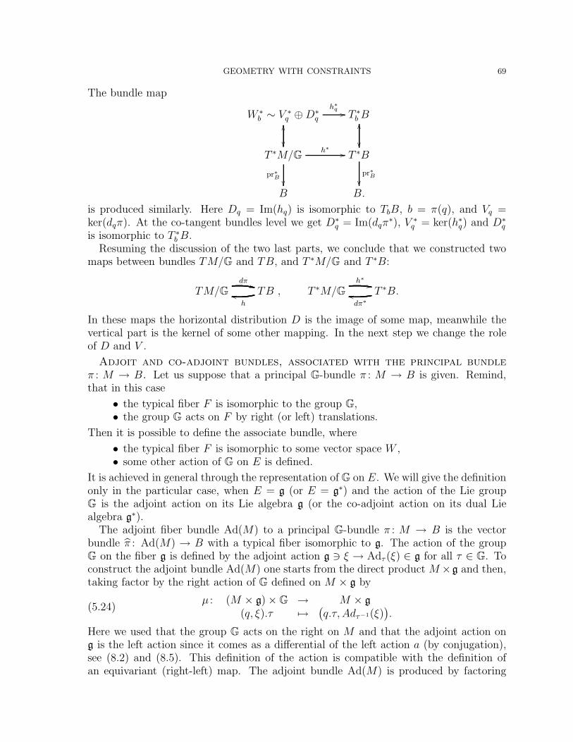
GEOMETRY WITH CONSTRAINTS 69
The bundle map
W ∗b ∼ V ∗
q ⊕D∗q
''
h∗q!! T ∗b B
''
T ∗M/G
((
pr∗B''
h∗ !! T ∗B
((
pr∗B''
B B.
is produced similarly. Here Dq = Im(hq) is isomorphic to TbB, b = π(q), and Vq =ker(dqπ). At the co-tangent bundles level we get D∗
q = Im(dqπ∗), V ∗
q = ker(h∗q) and D∗q
is isomorphic to T ∗b B.Resuming the discussion of the two last parts, we conclude that we constructed two
maps between bundles TM/G and TB, and T ∗M/G and T ∗B:
TM/Gdπ
**TB
h++ , T ∗M/G
h∗,,T ∗B.
dπ∗++
In these maps the horizontal distribution D is the image of some map, meanwhile thevertical part is the kernel of some other mapping. In the next step we change the roleof D and V .
Adjoit and co-adjoint bundles, associated with the principal bundleπ : M → B. Let us suppose that a principal G-bundle π : M → B is given. Remind,that in this case
• the typical fiber F is isomorphic to the group G,• the group G acts on F by right (or left) translations.
Then it is possible to define the associate bundle, where
• the typical fiber F is isomorphic to some vector space W ,• some other action of G on E is defined.
It is achieved in general through the representation of G on E. We will give the definitiononly in the particular case, when E = g (or E = g∗) and the action of the Lie groupG is the adjoint action on its Lie algebra g (or the co-adjoint action on its dual Liealgebra g∗).
The adjoint fiber bundle Ad(M) to a principal G-bundle π : M → B is the vectorbundle π : Ad(M) → B with a typical fiber isomorphic to g. The action of the groupG on the fiber g is defined by the adjoint action g $ ξ → Adτ (ξ) ∈ g for all τ ∈ G. Toconstruct the adjoint bundle Ad(M) one starts from the direct product M ×g and then,taking factor by the right action of G defined on M × g by
(5.24)µ : (M × g)×G → M × g
(q, ξ).τ %→ (q.τ, Adτ−1(ξ)
).
Here we used that the group G acts on the right on M and that the adjoint action ong is the left action since it comes as a differential of the left action a (by conjugation),see (8.2) and (8.5). This definition of the action is compatible with the definition ofan equivariant (right-left) map. The adjoint bundle Ad(M) is produced by factoring
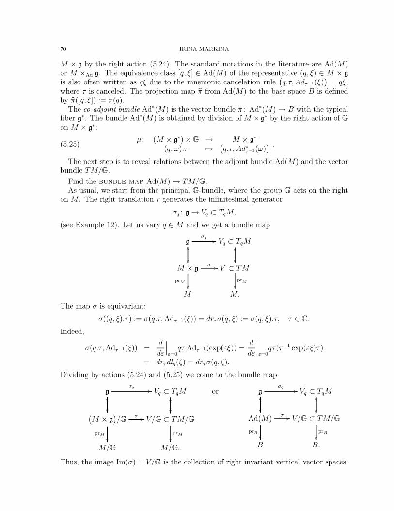
70 IRINA MARKINA
M × g by the right action (5.24). The standard notations in the literature are Ad(M)or M ×Ad g. The equivalence class [q, ξ] ∈ Ad(M) of the representative (q, ξ) ∈ M × gis also often written as qξ due to the mnemonic cancelation rule
(q.τ, Adτ−1(ξ)
)= qξ,
where τ is canceled. The projection map π from Ad(M) to the base space B is definedby π([q, ξ]) := π(q).
The co-adjoint bundle Ad∗(M) is the vector bundle π : Ad∗(M) → B with the typicalfiber g∗. The bundle Ad∗(M) is obtained by division of M × g∗ by the right action of Gon M × g∗:
(5.25)µ : (M × g∗)×G → M × g∗
(q,ω).τ %→ (q.τ, Ad∗τ−1(ω)
) ,
The next step is to reveal relations between the adjoint bundle Ad(M) and the vectorbundle TM/G.
Find the bundle map Ad(M) → TM/G.As usual, we start from the principal G-bundle, where the group G acts on the right
on M . The right translation r generates the infinitesimal generator
σq : g → Vq ⊂ TqM,
(see Example 12). Let us vary q ∈ M and we get a bundle map
g
''
σq!! Vq ⊂ TqM
''
M × g
((
prM
''
σ !! V ⊂ TM
((
prM
''
M M.
The map σ is equivariant:
σ((q, ξ).τ) := σ(q.τ, Adτ−1(ξ)) = drτσ(q, ξ) := σ(q, ξ).τ, τ ∈ G.
Indeed,
σ(q.τ, Adτ−1(ξ)) =d
dε
∣∣∣ε=0
qτ Adτ−1(exp(εξ)) =d
dε
∣∣∣ε=0
qτ(τ−1 exp(εξ)τ)
= drτdlq(ξ) = drτσ(q, ξ).
Dividing by actions (5.24) and (5.25) we come to the bundle map
g
''
σq!! Vq ⊂ TqM
''(M × g
)/G
((
prM
''
σ !! V/G ⊂ TM/G
((
prM
''
M/G M/G.
or g
''
σq!! Vq ⊂ TqM
''
Ad(M)
((
prB
''
σ !! V/G ⊂ TM/G
((
prB
''
B B.
Thus, the image Im(σ) = V/G is the collection of right invariant vertical vector spaces.
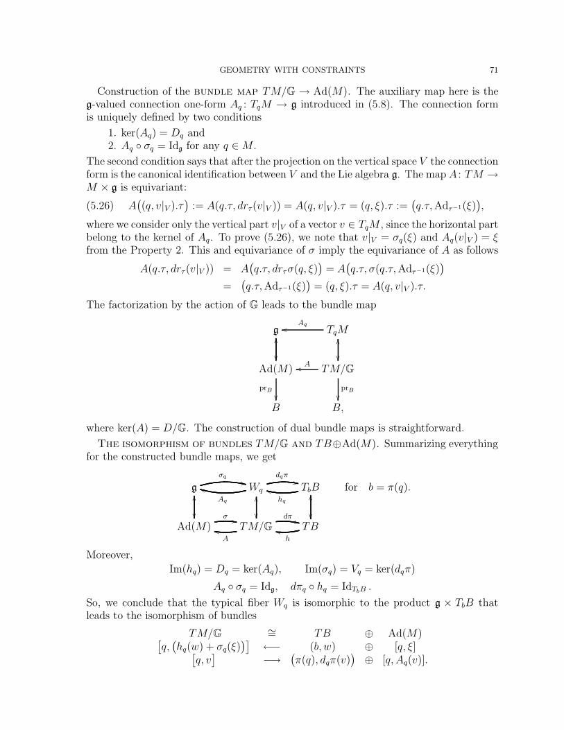
GEOMETRY WITH CONSTRAINTS 71
Construction of the bundle map TM/G → Ad(M). The auxiliary map here is theg-valued connection one-form Aq : TqM → g introduced in (5.8). The connection formis uniquely defined by two conditions
1. ker(Aq) = Dq and2. Aq σq = Idg for any q ∈ M .
The second condition says that after the projection on the vertical space V the connectionform is the canonical identification between V and the Lie algebra g. The map A : TM →M × g is equivariant:
(5.26) A((q, v|V ).τ
):= A(q.τ, drτ(v|V )) = A(q, v|V ).τ = (q, ξ).τ :=
(q.τ, Adτ−1(ξ)
),
where we consider only the vertical part v|V of a vector v ∈ TqM , since the horizontal partbelong to the kernel of Aq. To prove (5.26), we note that v|V = σq(ξ) and Aq(v|V ) = ξfrom the Property 2. This and equivariance of σ imply the equivariance of A as follows
A(q.τ, drτ(v|V )) = A(q.τ, drτσ(q, ξ)
)= A
(q.τ, σ(q.τ, Adτ−1(ξ)
)=
(q.τ, Adτ−1(ξ)
)= (q, ξ).τ = A(q, v|V ).τ.
The factorization by the action of G leads to the bundle map
g
''
TqM
''
Aq&&
Ad(M)
((
prB
''
TM/G
((
prB
''
A&&
B B,
where ker(A) = D/G. The construction of dual bundle maps is straightforward.
The isomorphism of bundles TM/G and TB⊕Ad(M). Summarizing everythingfor the constructed bundle maps, we get
g
σq**
''
Wq
Aq
--
dqπ,,
''
TbBhq
..
''
Ad(M)σ //
((
TM/Gdπ
**
((
A++ TB
h++
((for b = π(q).
Moreover,
Im(hq) = Dq = ker(Aq), Im(σq) = Vq = ker(dqπ)
Aq σq = Idg, dπq hq = IdTbB .
So, we conclude that the typical fiber Wq is isomorphic to the product g × TbB thatleads to the isomorphism of bundles
TM/G ∼= TB ⊕ Ad(M)[q,(hq(w) + σq(ξ)
)] ←− (b, w) ⊕ [q, ξ][q, v
] −→ (π(q), dqπ(v)
) ⊕ [q, Aq(v)].
72 IRINA MARKINA
Here hq(w) ∈ Dq is the horizontal lift of w ∈ Tπ(q)B and σq(ξ) ∈ Vq is a vector field.The result dqπ(v) represents the horizontal part of v ∈ TqM and Aq(w) is the missingvertical part regarded as an element of g. Let us emphasize one more time that theconstructed bundle isomorphism is induced by chosen Ehresmann connection D that isinvariant under the action of the structural group G.
Remark 7. Let us present the gauge group Gau(M) acting on the principal G-bundleπ : M → B. To do this, let us recall that a section of a fiber bundle ϕ : E → B is anyfunction f : B → E satisfying ϕ f = IdB. The bundle isomorphism σ : Ad(M) ↔V/G ⊂ TM/G gives a correspondence between the set S of all sections of the adjointbundle π : Ad(M) → B and the set L of G invariant vertical vector fields on M , sincethe set L is the set of sections of the bundle π : V/G → B. Thus the bundle map σinduces the isomorphism σ : S ↔ L.
Another observation: if there is a G-invariant map Φ : M →M , then factorization bythe action of the group G induces the map Φ : M/G = B →M/G = B.
Definition 24. The gauge group Gau(M) of the principal G-bundle π : M → B is the
set of all G-invariant maps Φ : M → M such that the induced map Φ is the identity on
B: Φ = IdB.
The Lie algebra gau(M) for the gauge group Gau(M) is the set of G-invariant vectorfields on M , which is exactly the set L, which is σ-isomorphic to S. Conclusion: thesections of the adjoint bundle Ad(M) form the Lie algebra of the gauge group.
We are actually interested in working with the dual isomorphism T ∗M/G ∼= T ∗B ⊕Ad∗(M), where in the construction of the co-adjoint action on g∗ and dual maps σ∗, A∗
to σ, A are used. Roughly speaking, the bundle isomorphism T ∗M/G ∼= T ∗B⊕Ad∗(M)is the splitting of the reduced phase space into the vertical part encoded in Ad∗(M)(generated by the action of G) and the complementary horizontal part isomorphic toT ∗B.
5.4.2. The Wong equation. The main goal of this part is to introduce the geodesic equa-tion on the reduced space T ∗M/G. To do this we need to introduce the curvatureform Ω of the Ehresmann connection D and the covariant derivative for sections on theco-adjoint bundle Ad∗(M).
Curvature form. A curvature two-form Ω on M associated with the Ehresmannconnection D measures the behavior of two horizontal vector fields X, Y ∈ D withrespect to each other, or more precise, Ω maps a pair X, Y ∈ ∧2 D to a vector (−[X, Y ]mod D) ∈ V . Since the connection one-form A gives an identification of V with the Liealgebra g, we define the g-valued two-form Ωq by
Ωq(X, Y ) =
−Aq([X, Y ]) if X, Y ∈ Dq,
0 othewise,for all q ∈ M.
Since the form A is defined on G- invariant vector fields, we get−A([X, Y ]) = dA(X, Y )−[A(X), A(Y )] and we conclude that
Ω = dA− [A, A].
GEOMETRY WITH CONSTRAINTS 73
The form Ω is G-equivariant, since the form A is so. The equivariance of Ω allows toextend the definition of Ω to the bundle map∧2 Dq
''
Ωq!! g
''∧2 D
((
prM
''
Ω !! M × g
((
prM
''
M M
=⇒ factoring by G =⇒ ∧2 Dq
''
Ωq!! g
''(∧2 D)/G
((
prB
''
Ω !! Ad(M)
((
prB
''
B B.
The last property is reflected in the name of the curvature two-form Ω as Ad(M)-valuedcurvature form.
Covariant derivative for sections on the co-adjoint bundle Ad∗(M).Let ψ : B → Ad(M) be a section, and X ∈ Vect B, then we would like to define thecovariant derivative DXψ that for any chosen ψ and X gives the section of the adjointbundle Ad(M) that is DXψ : B → Ad(M).
To define it we first relate a map F : M → g to ψ by the following
B $ bψ−→ (q, ξ) = (q, F (q)) ∈ Ad(M),
where b = π(q), q ∈ M , and ξ = F (q) ∈ g. The map F should be equivariant:F (q.τ) = F (q).τ = Adτ−1(F (q)), since ψ is equivariant by definition.
The differential mapdqF : TqM → TF (q)g ∼= g
(q, v) %→ (q, dqF (v))
leads to the bundle map dF : TM →M × g. If we show that dF is equivariant, then bytaking factor by the action of group, we get a bundle map
dF : TM/G → Ad(M)
that sends any point (q, Y ), with q ∈ M and Y being a G-invariant vector field, to thepoint (q, dqF (Y )) ∈ Ad(M), where F : M → g is equivariant. But q ∈ M is such thatπ(q) = b ∈ B, and Y is the horizontal lift by h of some vector field X ∈ Vect B. Sogiven b ∈ B, X ∈ Vect B, the composition dF (h X) is the desired section
ψ : BX→ TB
h→ TM/G dF→ Ad(M).
The following chain of equalities shows that dF : TM → M × g is equivariant
dF (q.τ, drτh(X)) =(q.τ, dFq.τ(hX(q.τ))
)= dF (q, h(X)).τ
due to the equivarience of F .
The Wong equation. Let c : I → B be a curve on the base space, that representsthe trajectory of the motion of some charged particle. Then c(t) ∈ Vect B is the vectorfield along c and the horizontal lift h sends this vector field to Dγ(t) ⊂ Tγ(t)M , or
T(c(t))B $ (c(t), c(t))h→ (γ(t), h(c(t))) ∈ Dγ(t)Tγ(t)M, π(γ(t)) = c(t).
74 IRINA MARKINA
The contraction icΩ of Ad(M)-valued two-form Ω on h(c) is Ad(M)-valued one-formalong c:
icΩ(·) := Ω(h(c), ·) : TB → Ad(M).
Take any section λ(t) = λ(c(t)) of the co-adjoint bundle Ad∗(M) along the curve c onthe base space: λ : B → Ad∗(M). The section λ representsthe charge (electromagneticor color-charge) of a particle moving in B. The duality of Ad(M) and Ad∗(M) producesa momentum in T ∗B, by
Λc,Ω(·) := 〈λ(c(t)), icΩ(·)〉.The pairing 〈·, ·〉 associates to each vector field X ∈ TB a real number given by thepairing between λ(c(t)) ∈ Ad∗(M) and ic(t)Ω(h(X)) ∈ Ad(M) along the curve c. ThusΛc,Ω ∈ T ∗B. Now we exploit the Riemannian metric gB given on the base space B and
find the canonical dual Λ#c,Ω ∈ TB to Λc,Ω. The vector field Λ#
c,Ω represents a force actingon the base space B produced by the charge λ of the particle. This force is called theLorentz force
The presence of the non-abelian Lorentz force Λ#c,Ω leads to the equation called the
Wong equation,
(5.27) ∇cc = Λ#c,Ω,
where the non-abelian charge λ has to satisfy the condition
(5.28) Dc(t)λ(c(t)) = 0, for any t ∈ I.
expressing the property that the charge has to be “co-variantly constant” along c.The second order differential equations (5.27) and (5.28) have the solution that is the
curve (c(t),λ(c(t))) ∈ Ad∗(M), t ∈ I, in the co-adjoint bundle lying over the curve c inthe base space B. The system of equations can be rewritten as the first order systemon T ∗B⊕Ad∗(M) by introducing the momentum p(t) = p(c(t)) ∈ T ∗c(t)B along the base
curve c. We again use the metric tensor gB and define the co-vector p(t)(·) = gB(c(t), ·).Then (p,λ) ∈ T ∗B ⊕ Ad∗(M).
Since we have the isomorphism TM/G ∼= T ∗B⊕Ad∗(M), the solution (p,λ) on T ∗B⊕Ad∗(M) is also solution on TM/G. The following theorem is an analogue of Theorem 5.1produced for the case 2 and it expresses the relation between sub-Riemannian geodesicsin Case 2 and the solutions of the Wong equations.
Theorem 5.2. [94] Let Γ = (γ, p) be a normal sub-Riemannian bi-characteristic for(M, D, gD), produced by the principal G-bundle π : M → B, where sub-Riemannianstructure (D, gD) is G-invariant and gD is the pullback of the Riemannian metric gB
on B. The projection of Γ onto TM/G ∼= T ∗B ⊕ Ad∗(M) is the solution of the Wongequations (5.27) and (5.28).
Conversely, let c(t) ∈ B, t ∈ I, be a solution of the Wong equation (5.27) com-plemented by (5.28) and h(c(t)) be its horizontal lift to M . Then h(c(t)) is a normalsub-Riemannian geodesic for (M, D, gD) described as above. The non-abelian chargeλ ∈ Ad∗(M) corresponds to the co-vector p ∈ T ∗M .
Instead of presenting the proof of the theorem, that can be found in [94], we showthe relation between this theorem and the examples of Carnot groups considered inSection 3.
GEOMETRY WITH CONSTRAINTS 75
5.5. Examples of solutions to the Wong equations. Before we present the exam-ples, let us do some observations about the Wong equation (5.27).
Conservation of energy. By definition, Λ#c,Ω(v) = 〈λ(c(t)),Ω(h(c), h(v))〉. Since
the form Ω is skew symmetric, then for v = c we get Λ#c,Ω(c) = 0 that leads to 〈∇cc, c〉 = 0
by the Wong equation (5.27). Since the derivative of the kinetic energy is ddt
(12〈c, c〉
)=
〈∇cc, c〉 = 0, we conclude that the kinetic energy is constant along solutions of (5.27).This energy is equal to the value of the sub-Riemannian Hamiltonian function along thecorresponding sub-Riemannian geodesic.
Relation to physics. If the group G acting on M is abelian, then the Wongequations are known as the Lorentz equations. In this case the adjoint bundle Ad∗(M) isthe trivial bundle M×g∗, where elements of the fiber g∗ represent charges. The conditionof the covariant constancy (5.28) asserts that the charge λ(t) is constant. The rest (5.27)is the family of equations, parametrized by the charge. These sub-Riemannian geodesics,corresponding to the bundle type structures project to the motion of a particle on thebase manifold B under the influence of the magnetic field Ω, defined by the curvature ofthe horizontal distribution D. We get a family of curves parametrized by the charge λ.This observation is one of the main parts of the Kaluza-Klein theory. The Lorentzequations play an important role in classical electrodynamics and both the classical andquantum versions of electromagnetism are highly successful physical theories.
The quantum versions of non-abelian gauge theory are quite successful and activelydeveloping subject as we discussed at the beginning of the section. The interesting pe-culiarity, that in contrast to the abelian electromagnetic case, the non-abelian quantumtheory has no physically meaningful classical analogue, or in other words, there are nosuch thing as a classical quark (non-abelian electron), or classical gluon (non-abelianphoton). It seems that the non-abelian Lorentz equations have no useful physical appli-cations in high energy particle theory, but they found their impact on the mechanicalsystems such as falling, swimming, orbiting, and rolling. In the next section we get adescription of the rolling system of two bodies, leaving out other applications apart.The reader can find interesting examples of principal bundles associated to mechanicalsystems in [94].
5.5.1. Heisenberg group. The Heisenberg manifold. Let B = R2 be the base space,where an electrically charged particle will move. Assume that B is endowed with theusual Euclidean metric and we will use the standard coordinate system b = (x, y). Letπ : M = R3 → B, be the principle R-bundle, where π = pr1,2 is the projection on theplane formed by two first coordinates. The action of the structure group G = (R, +) isdefined by
µ : R3 × R → R3
(x, y, t).τ %→ (x, y, t + τ).
The vertical space is Vq = ker(π) = span∂t. Let us chose the horizontal distributionD = span∂x, ∂y. Then the connection R-valued one-form is just A = dt and thecurvature form Ω = −dA ≡ 0. We see that there is no magnetic field and the motionis a free motion on the base space, or its copy. Geodesics are straight lines. The sub-Riemannian metric gD, which is the pullback of the Euclidean metric, is the Euclidean
76 IRINA MARKINA
metric on D. The distribution D is orthogonal to V with respect to the Euclideanmetric in R3, it is not bracket generating, the sub-Riemannian manifold (R3, D, gD) isthe foliation by planes t = constant, and the motion is possible only inside of a planedefined by the initial position of the particle.
We choose now the horizontal distribution in another, non-trivial way, for instanceD = spanX, Y , where
X = ∂x, Y = ∂y + x∂t,
or in a more symmetric way
X = ∂x − 1
2y∂t, Y = ∂y +
1
2x∂t.
In this case the reader recognizes the Heisenberg distribution. Since
dπ(X) = ∂x, dπ(Y ) = ∂y,
the pullback of the Euclidean metric from R2 to D is represented by the identity matrixand makes the vector fields X, Y into the orthonormal basis of D. The connection formis A = dt − 1
2xdy + 1
2ydx and, as we remember, it is the dual form to the vertical
vector field T = ∂t. The vector fields X, Y, T and their commutation relations define theHeisenberg group structure in R3 through the BCH-formula (8.1).
The curvature form Ω = −dA = dx∧dy is constant, non-vanishing and is equal to thevolume form on R2. Any form Ω = F (x, y)dx∧dy represents a magnetic field in the basespace B = R2, that also can be thought as a field 0 dy ∧ dt + 0 dt ∧ dx + F (x, y)dx∧ dyorthogonal to the base space B. As it is known, in order to be a magnetic field the formΩ has to satisfy the Maxwell equation dΩ = 0, which is true in this case. Observe thatin the presence of the abelian structure group the curvature form given by Ω = −dA(since [A, A] = 0 in this case) automatically satisfies the Maxwell equation. In the caseF (x, y) = constant the magnetic field coincides up to a constant with the Heisenbergcurvature form.
Let us have a look on the Lorentz equation (5.27). The Lie algebra of the structuregroup is R and the dual to it is also R. Thus, the co-adjoint bundle is a trivial bundlewith the typical fiber R. The covariant derivative is the usual derivative and we get thatthe charge λ has to be constant by (5.28). The horizontal lift h maps the velocity vectorc = x∂x + y∂y ∈ TcR2 to c = xX(c) + yY (c) ∈ Dc. Moreover,
∇cc = c, icΩ = Ω(c),
and the Lorentz equation becomes
c = −λΩ(c).
The last equation coincides with the Hamiltonian equation (3.6) with θ0 = λ. So,geodesics produced by these equations are the Heisenberg geodesics described in Sub-section 3.2.
Heisenberg manifold and S3 with the Kahler structure. Suppose that weare given as the base space a manifold B, endowed with the Kahler structure. Let usremind the definition of a Kahler manifold.
GEOMETRY WITH CONSTRAINTS 77
Definition 25. Let M be a complex integrable manifold with corresponding complexstructure J . We say that a Riemannian metric gM is compatible with J if
gM(v, w) = gM(Jv, Jw), for all v, w ∈ TqM, q ∈ M.
The triplet (M, J, gM) is called an Hermitian manifold. The compatible J and gM
defines a skew symmetric form ω by
(5.29) ω(v, w) := gM(Jv, w) for all v, w ∈ TqM, q ∈ M
and it is called the associated Kahler form. We can retrieve gM from ω also.
Definition 26. A Kahler manifold is a complex integrable manifold M endowed withthe complex structure J , compatible Riemannin metric gM , associated Kahler form ω,such that dω = 0.
It is important for us to know that the Kahler form ω and the Riemannian metricgM are related by (5.29). We suppose that the curvature form Ω is given by the Kahlerform ω. The Lorentz equation becomes
∇cc = −λJc(c).
We recognize the variational equations (3.16) and (5.15) obtained by variational methodsfor the Heisenberg group and for the Hopf fibration on S3. Observe that the Levi-Civitaconnections in (3.16) and (5.15) are connections related to Riemannian metrics on thetotal space M and the solutions γ are the sub-Riemannian geodesics on M . Meanwhile,the Levi-Civita connection in the Lorentz equation is the connection related to theRiemannian metric on the base space B and the solution is a curve c in the base space,parameterized by the charge. However, projections of γ coincide with c, as was assertedin Theorem 5.2.
Curvature of geodesics on surfaces. Let B be an oriented surface (two di-mensional manifold) furnished with a Riemannian metric gB. Let ω be its area form.The equation ω(v, w) = ω(Jv, w) for v, w ∈ TbB defines an almost complex structureJb : TbB → TbB on B.
Consider a principle U(1)-bundle π : M → B over B. The curvature form Ω canbe written as Ω = Fω for some F ∈ C∞(B). The scalar field F or the endomorphismFJ : TB → TB defines the magnetic field acting on the surface B. The Lorentz equationbecomes
∇cc = −eFJc(c), e is a constant charge.
Suppose that the geodesic c is parametrized by arc length: gB(c, c) = 1. The geodesiccurvature kgeod(t) along c is defined by kgeod(t) = gB(Jc(c),∇cc) and the Lorentz equationis equivalent to
kgeod(t) = eF (c(t)).
Suppose now that the magnetic field F is constant, that leads to the constant geodesiccurvature. Thus, if the base space B is the plane then the geodesics are circles, whichcoincides with the Heisenberg case. If B is the two dimensional sphere S2, then geodesicswill be great circles and this is reflected in the picture of the Hopf fibration S3 over S2.
78 IRINA MARKINA
5.5.2. Quaternionic H-type group with the Lorentzian metric. In this example we takeas the base space B the Minkowski space R3,1 = (R4, gB), where gB is a non-degeneratemetric tensor of index 1 having the associated matrix
−1 0 0 00 1 0 00 0 1 00 0 0 1
.
Define the principal R3-bundle π : R4+3 → R4 with the standard projection into the fourdimensional subspace, where the abelian group (R3, +) acts by
µ : R7 × R3 → R7
(b, t1, t2, t3).(τ1, τ2, τ3) → (b, t1 + τ1, t2 + τ2, t3 + τ3),b ∈ R4.
Analogously to the Heisenberg manifold we find the vertical space Vq, q = (b, t1, t2, t3)by V = span∂t1 , ∂t2 , ∂t3. We chose the horizontal distribution D as the span of X11,X21, X31, X41 in (3.31). With this we get the Ehresmann connection and recuperatethe structure of quaternionic H-type group of the lowest dimension. The choice of thebasis for D is completely defined by the choice of almost complex structures (3.29). Thepullback of the Minkowski metric is now a non-degenerate metric of index 1, convertingthe vector fields X11, X21, X31, X41 into an orthonormal basis and defining the first oneX11 as a globally defined timelike vector field. The corresponding geometry can be calledthe sub-Lorentzian geometry. Different types of sub-Lorentzian manifolds were studiedin [25, 49, 50, 73, 74, 75].
The curvature form Ω defines an R3-valued constant magnetic field. The projections ofsub-Lorentzian geodesics into the Minkowski base space are divided into three differentcausal type and were considered in details in [74].
The change of principle R3-bundle to the bundle π : B × S1 → B, B = R3,1, wherethe abelian group U(1) acts on the slot S1 by the standard multiplication of complexnumbers, leads to the classical Kaluza-Klein model.
Exercise
1. Consider a round version of the Heisenberg group H1 ∼= R3 = R2×S1 as principalU(1)-bundle, where the action is defined by
(R2 × S1)× U(1) → R2 × S1
(x, y, eiϕ).υ %→ (x, y, eiϕ.υ).
Find a horizontal distribution with non-trivial curvature form. Write basic vectorfields for the horizontal distribution and find the commutation relation betweenthem. Do they form the Heisenberg algebra? If yes, find the group multiplicationlaw in R3 by making use BCH-formula.
2. Construct Kaluza-Klein model, associated with two-step Carnot groups in Sub-section 3.4.
6. Rolling manifolds
Rolling surfaces without slipping or twisting is one of the classical kinematic problemsthat in recent years has again attracted attention of mathematicians due to its geometric
GEOMETRY WITH CONSTRAINTS 79
and analytic richness. The kinematic conditions of rolling without slipping or twistingare described by means of motion on a configuration space being tangential to a smoothsub-bundle of the tangent bundle ot the configuration space that we call, as before, thehorizontal distribution. The precise definition of the mentioned motion in the case of twon-dimensional manifolds imbedded in RN , given for example in [107], involves studyingthe behavior of the tangent bundles of the manifolds and the normal bundles inducedby the imbeddings. This extrinsic point of view, which depends on the imbeddings,has been successfully applied, for instance in [57, 58]. The drawback of the extrinsicapproach is that the geometric descriptions depend strongly on the imbedding underconsideration.
So far, few attempts have been made to formulate this problem intrinsically. Anearly enlightening formulation is given in [17], that is achieved by means of an intrinsic
version of the moving frame method of Elie Cartan, see [22, 108]. One of the importantresults established there is the bracket generating property of the rank two distributioncorresponding to no-twisting and no-slipping restrictions, namely, if the two surfaceshave different Gaussian curvature, then the distribution is bracket generating, see [17].A control theoretic approach to the same problem, studied in [3], has the advantagethat the kinematic restrictions are written explicitly as vector fields on the appropriateconfiguration space.
We present here a short description of a generalization of the kinematic problem fortwo n-dimensional abstract manifolds rolling without twisting or slipping via an intrin-sic formulation. We define the configuration space of the system, present an extrinsicdefinition of rolling for manifolds imbedded into the Euclidean space, several equiva-lent definitions of rolling, involving intrinsic characteristics, and discuss their relations.The intrinsic approach permits to determine the imbedding-independent informationcontained in the extrinsic definition.
6.1. Extrinsic rolling. Let M and M be oriented, connected, n-dimensional Riemann-ian manifolds isometrically imbedded into Rn+ν , equipped with the standard Euclideanmetric and standard orientation. Isometrical imbeddings always exist due to a result ofNash [97] and we denote them by ι and ι, respectively. The corresponding Riemannian
metrics on M and M coincide with the restrictions of the Euclidean metric from Rn+ν
and they will be denoted by gM and gM .
Objects (points, curves, . . . ) related to the manifold M will be marked by a hat ()on top, objects related to M will be free of it, while those related to the ambient spaceRN , N = n + ν, will carry a bar ( − ).
Note that for any manifold M imbedded in Rn+ν , there is a natural splitting of thetangent space of Rn+ν into a direct sum:
(6.1) TxRn+ν = TxM ⊕ TxM⊥, x ∈ M,
where TxM is the tangent space and TxM⊥ is normal space to M at x. According to
the splitting (6.1), any vector v ∈ TxRn+ν , x ∈ M , can be written uniquely as the sumv = v( + v⊥, where v( ∈ TxM , v⊥ ∈ TxM
⊥. Analogous projections can be defined
for M .
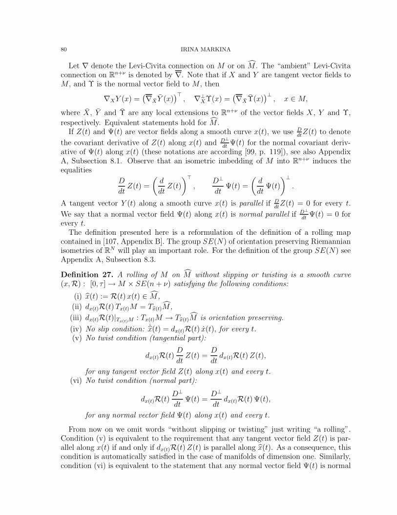
80 IRINA MARKINA
Let ∇ denote the Levi-Civita connection on M or on M . The “ambient” Levi-Civitaconnection on Rn+ν is denoted by ∇. Note that if X and Y are tangent vector fields toM , and Υ is the normal vector field to M , then
∇XY (x) =(∇X Y (x)
)(, ∇⊥XΥ(x) =
(∇XΥ(x))⊥
, x ∈ M,
where X , Y and Υ are any local extensions to Rn+ν of the vector fields X , Y and Υ,
respectively. Equivalent statements hold for M .If Z(t) and Ψ(t) are vector fields along a smooth curve x(t), we use D
dtZ(t) to denote
the covariant derivative of Z(t) along x(t) and D⊥dtΨ(t) for the normal covariant deriv-
ative of Ψ(t) along x(t) (these notations are according [99, p. 119]), see also AppendixA, Subsection 8.1. Observe that an isometric imbedding of M into Rn+ν induces theequalities
D
dtZ(t) =
(d
dtZ(t)
)(,
D⊥
dtΨ(t) =
(d
dtΨ(t)
)⊥.
A tangent vector Y (t) along a smooth curve x(t) is parallel if Ddt
Z(t) = 0 for every t.
We say that a normal vector field Ψ(t) along x(t) is normal parallel if D⊥dtΨ(t) = 0 for
every t.The definition presented here is a reformulation of the definition of a rolling map
contained in [107, Appendix B]. The group SE(N) of orientation preserving Riemannianisometries of RN will play an important role. For the definition of the group SE(N) seeAppendix A, Subsection 8.3.
Definition 27. A rolling of M on M without slipping or twisting is a smooth curve(x,R) : [0, τ ] →M × SE(n + ν) satisfying the following conditions:
(i) x(t) := R(t) x(t) ∈ M ,
(ii) dx(t)R(t) Tx(t)M = Tx(t)M ,
(iii) dx(t)R(t)|Tx(t)M : Tx(t)M → Tx(t)M is orientation preserving.
(iv) No slip condition: ˙x(t) = dx(t)R(t) x(t), for every t.(v) No twist condition (tangential part):
dx(t)R(t)D
dtZ(t) =
D
dtdx(t)R(t) Z(t),
for any tangent vector field Z(t) along x(t) and every t.(vi) No twist condition (normal part):
dx(t)R(t)D⊥
dtΨ(t) =
D⊥
dtdx(t)R(t)Ψ(t),
for any normal vector field Ψ(t) along x(t) and every t.
From now on we omit words “without slipping or twisting” just writing “a rolling”.Condition (v) is equivalent to the requirement that any tangent vector field Z(t) is par-allel along x(t) if and only if dx(t)R(t) Z(t) is parallel along x(t). As a consequence, thiscondition is automatically satisfied in the case of manifolds of dimension one. Similarly,condition (vi) is equivalent to the statement that any normal vector field Ψ(t) is normal
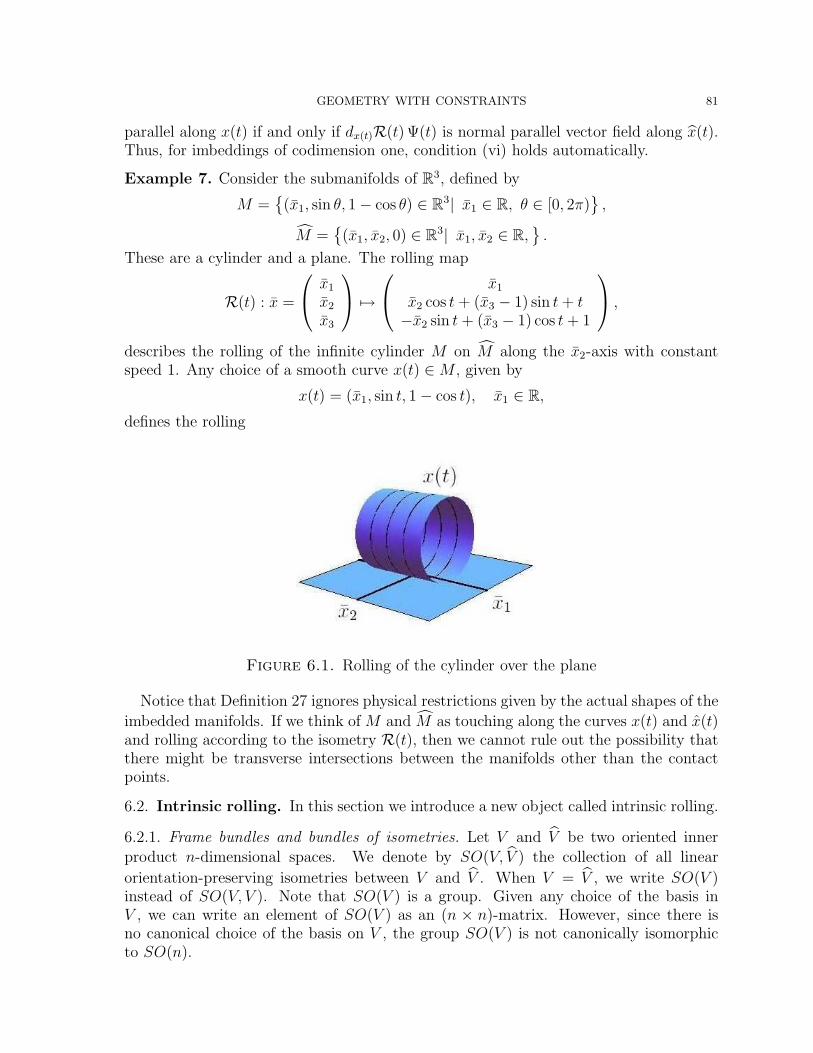
GEOMETRY WITH CONSTRAINTS 81
parallel along x(t) if and only if dx(t)R(t)Ψ(t) is normal parallel vector field along x(t).Thus, for imbeddings of codimension one, condition (vi) holds automatically.
Example 7. Consider the submanifolds of R3, defined by
M =(x1, sin θ, 1− cos θ) ∈ R3| x1 ∈ R, θ ∈ [0, 2π)
,
M =(x1, x2, 0) ∈ R3| x1, x2 ∈ R,
.
These are a cylinder and a plane. The rolling map
R(t) : x =
x1
x2
x3
%→ x1
x2 cos t + (x3 − 1) sin t + t−x2 sin t + (x3 − 1) cos t + 1
,
describes the rolling of the infinite cylinder M on M along the x2-axis with constantspeed 1. Any choice of a smooth curve x(t) ∈ M , given by
x(t) = (x1, sin t, 1− cos t), x1 ∈ R,
defines the rolling
Figure 6.1. Rolling of the cylinder over the plane
Notice that Definition 27 ignores physical restrictions given by the actual shapes of the
imbedded manifolds. If we think of M and M as touching along the curves x(t) and x(t)and rolling according to the isometry R(t), then we cannot rule out the possibility thatthere might be transverse intersections between the manifolds other than the contactpoints.
6.2. Intrinsic rolling. In this section we introduce a new object called intrinsic rolling.
6.2.1. Frame bundles and bundles of isometries. Let V and V be two oriented innerproduct n-dimensional spaces. We denote by SO(V, V ) the collection of all linear
orientation-preserving isometries between V and V . When V = V , we write SO(V )instead of SO(V, V ). Note that SO(V ) is a group. Given any choice of the basis inV , we can write an element of SO(V ) as an (n × n)-matrix. However, since there isno canonical choice of the basis on V , the group SO(V ) is not canonically isomorphicto SO(n).
82 IRINA MARKINA
For any pair M and M , we introduce the space Q of all relative positions in which M
can be tangent to M
(6.2) Q =
q ∈ SO(TxM, TxM)∣∣∣ x ∈ M, x ∈ M
.
This space is a manifold with a structure of an SO(n)−fiber bundle over M×M and can
be considered as the configuration space of the rolling. Its dimension is n(n+3)2
. Notice,that it is not a principal SO(n)−bundle since the action of SO(n) on the fiber depend
on the choice of coordinates in M and M . To see this in more detail, we describe the
space Q in terms of frame bundles. Let F and F be the oriented orthonormal frame
bundles of M and M , respectively. As we know from Subsection (8.5.1) of Appendix A,
F and F are principal SO(n)-bundles.
Consider F × F as a bundle over M × M . The group SO(n) acts on the right on F
and F and we can divide by this action diagonally on fibers. Then, we can identify Q
with (F × F )/SO(n) by the map assigning to each equivalence class [f, f ] the mappingq ∈ Q, such that
(6.3) fj = q fj , for j = 1, . . . , n.
Clearly, this construction does not depend on the choice of a representative of an equiv-
alence class of (F × F )/SO(n). Conversely, given an isometry q ∈ Q, there exists aunique equivalence class of frames satisfying (6.3).
As we see, we can define the right action by SO(TxM) or the left action by SO(TxM)
on (F × F )/SO(n). Since both groups are not canonically isomorphic to SO(n) (except
for the case when n = 2), the configuration space Q = (F × F )/SO(n) does not have thestructure of a principal SO(n)−bundle. However, since Q is an SO(n)−fiber bundle we
can exploit its local properties and think that it looks locally like the product M × M ×SO(n). Let U be a neighborhood in M such that F |U is trivial and let v be a section ofF |U : v(x) = (v1(x), . . . , vn(x)), x ∈ M . Each section determines a left action of SO(n)on F |U . To see this, recall that for each x ∈ U , the frame v(x) can be considered as anisometry v(x) : Rn → TxM . The left action takes the following form: if f ∈ Fx is anyother frame at x ∈ U , written in terms of the frame v as
fj =
n∑i=1
fijvi(x),
then τ = (τij)ni,j=1 ∈ SO(n) acts on the left on f via the equation
τ.fj =n∑
i,k=1
fijτkivk, j = 1, . . . , n.
Observe that this action depends on the choice of the frame v.
This defines local left and right actions of SO(n) on Q as follows. Let U and U be
neighborhoods in M and M respectively, so that both frame bundles trivialize over these
neighborhoods. Let v : U → F |U and v : U → F |U be sections. We define the left action
GEOMETRY WITH CONSTRAINTS 83
of τ ∈ SO(n) on Q with respect to v by
τ.fj = (τ.q)fj,
where the left action of τ on fj is defined with respect to v and fj = qfj for j = 1, . . . , n.Similarly, the right action of SO(n) on Q with respect to v is defined by
fj = (q.τ)(τ−1.fj
).
Remark that if we have a matrix representation of an element τ0 ∈ SO(n) in coordi-
nates of M by τ0 =gM(vi, qvj)
n
i,j=1, then we have
gM(vi, (τ.q)vj)n
i,j=1= ττ0, and
gM(vi, (q.τ)vj)
n
i,j=1= τ0τ, τ ∈ SO(n).
6.2.2. Reformulation of rolling in terms of bundles. Both formulations of rolling surfacesgiven in [3, 17] define the configuration space as a manifold of isometries of tangent
spaces of M and M , as we did before, without taking into account the imbedding intothe ambient space. The condition (vi) imposed over a rolling (x,R) by Definition 27is non-trivial whenever the codimension ν of the imbedded manifolds is greater than 1.So, it is natural to suppose that the total configuration space of the rolling system willhave a normal component which takes care of the action of R on the normal bundle.
Therefore, by analogy with the construction of Q, we define a fiber bundle over M × M
of isometries of the normal tangent space. Let ι : M → Rn+ν and ι : M → Rn+ν be twoimbeddings, given as initial data. Let Φ be the principal SO(ν)−bundle over M , suchthat the fiber over a point x ∈ M consists of all positively oriented orthonormal frames
ελ(x)νλ=1 spanning TxM⊥. Let Φ be the similarly defined principal SO(ν)−bundle
on M . As it was done previously, we identify the manifold (Φ× Φ)/SO(ν) with
(6.4) Pι,ι :=
p ∈ SO(TxM⊥, TxM
⊥)∣∣∣ x ∈ M, x ∈ M
.
The space Pι,ι is not in general a principal SO(ν)−bundle, but there are local left andright actions defined similarly as on Q. We notice and reflect it in notations that Q is
invariant of imbeddings, while Pι,ι is not. The dimension of Pι,ι is 2n + ν(ν−1)2
.
We form the direct sum Q ⊕ Pι,ι for the fiber bundle over M × M , so that the fiber
over (x, x) ∈ M × M , is Q(x,x) × Pι,ι(x,x). The dimension of Q⊕ Pι,ι is n(n+3)+ν(ν−1)2
.The following proposition allows to reformulate Definition 27.
Proposition 9. If a curve (x,R) : [0, τ ] → M × SE(n + ν) satisfies the conditions(i)-(vi) in Definition 27, then the mapping
t %→ (dx(t)R(t)|Tx(t)M , dx(t)R(t)|Tx(t)M⊥) =: (q(t), p(t)) ,
defines a curve in Q⊕ Pι,ι with the following properties:
(I) no slip condition: ˙x(t) = q(t)x(t) for every t.(II) no twist condition, tangential part: q(t)D
dtZ(t) = D
dtq(t)Z(t) for any tangent vector
field Z(t) along x(t) and every t.
(III) no twist condition, normal part: p(t)D⊥dtΨ(t) = D⊥
dtp(t)Ψ(t) for any normal vector
field Ψ(t) along x(t) and every t.
84 IRINA MARKINA
Conversely, if (q, p) : [0, τ ] → Q⊕Pι,ι is a smooth curve satisfying (I)-(III), then thereexists a unique rolling
(x,R) : [0, τ ] →M × SE(n + ν),
such that dx(t)R(t)|Tx(t)M = q(t) and dx(t)R(t)|Tx(t)M⊥ = p(t).
Proof. Assume that (x,R) : [0, τ ] → M × SE(n + ν) is a rolling map satisfying (i)-(vi).The conditions (i) and (ii) assure that
dx(t)R(t)|Tx(t)M ∈ SO(Tx(t)M, Tx(t)M) and
dx(t)R(t)|Tx(t)M⊥ ∈ SO(Tx(t)M⊥, Tx(t)M
⊥).(6.5)
Since dx(t)R(t) must be orientation preserving in Rn+ν we conclude that both of themappings (6.5) are either orientation reversing or orientation preserving. The additionalrequirement (iii) implies that (q, p) is orientation preserving. The conditions (I)-(III)correspond to the conditions (iv)-(vi).
Conversely, if we have a curve (q(t), p(t)) in Q⊕ Pι,ι with projection (x(t), x(t)) into
M × M , then we have an isometry R ∈ SE(n + ν) in the following way: R(t) : x %→A(t)x + a(t), A(t) ∈ SO(n + ν), where A(t) = dx(t)R(t) is determined by the conditions
dx(t)R(t)|Tx(t)M = q(t)|Tx(t)M , dx(t)R(t)|Tx(t)M⊥ = p(t)|Tx(t)M⊥.
Then for images of dx(t)R(t) we have
Im(dx(t)R(t)|Tx(t)M
)= Tx(t)M, Im
(dx(t)R(t)|Tx(t)M⊥
)= Tx(t)M
⊥.
The vector a(t) is determined by a(t) = x(t)− A(t)x(t). !
The one-to-one correspondence between rolling maps and smooth curves in Q ⊕ Pι,ι,satisfying (I)-(III), naturally leads to a definition of a rolling map in terms of thesebundles.
Definition 28. A rolling of M on M without slipping or twisting is a smooth curve(q, p) : [0, τ ] → Q⊕ Pι,ι such that (q(t), p(t)) satisfies
(I) no slip condition: ˙x(t) = q(t)x(t) for every t,(II) no twist condition, tangential part: q(t)D
dtZ(t) = D
dtq(t)Z(t) for any tangent vector
field Z(t) along x(t) and every t,
(III) no twist condition, normal part: p(t)D⊥dtΨ(t) = D⊥
dtp(t)Ψ(t) for any normal vector
field Ψ(t) along x(t) and every t.
Proposition 9 implies that the bundle Q⊕ Pι,ι can be seen as the configuration space
for a rolling. According to [107], the dimension n(n+3)+ν(ν−1)2
corresponds to the degreesof freedom of the system.
A purely intrinsic definition of a rolling is deduced from Definition 28, by restrictingit to the bundle Q. This concept naturally generalizes the definition given in [3] for2-dimensional Riemannian manifolds imbedded into R3 and we use the term intrinsicrolling for this object.
GEOMETRY WITH CONSTRAINTS 85
Definition 29. An intrinsic rolling of two n-dimensional oriented Riemannian man-
ifolds M on M without slipping or twisting is a smooth curve q : [0, τ ] → Q, withprojections x(t) = prM q(t) and x(t) = prM q(t), satisfying the following conditions:
(I’) no slip condition: ˙x(t) = q(t)x(t) for all t,(II’) no twist condition: Z(t) is a parallel tangent vector field along x(t), if and only ifq(t)Z(t) is parallel along x(t) for all t.
Remark 8. If the manifolds are imbedded into Euclidean space Rn+1, then for each pair
of points (x, x) ∈ M ×M , there is a unique orientation preserving isometry p : TxM⊥ →
TxM⊥. Hence, since Pι,ι is an SO(1)-bundle, it can be identified with M × M , and so
Q ⊕ Pι,ι∼= Q. In this case we see that the notion of rolling in Definition 28 coincides
with the intrinsic rolling in Definition 29.
6.2.3. Extrinsic and intrinsic rollings along the same curves. Let (x, x) : [0, τ ] →M×Mbe a fixed pair of curves which are projections of a rolling map. We aim to give an answerto the following questions:
• If (q1(t), p1(t)) and (q2(t), p2(t)) are two rollings of M on M , along x(t) and x(t), howare they related? What properties of the rolling are defined by fixing the paths x and x?
• Suppose an intrinsic rolling q(t) and imbeddings of M and M into Rn+ν are given. Isit possible to extend q(t) to a rolling (q(t), p(t))? Is this extension unique?
The following example clarifies the situation for one dimensional manifolds, wheredifferent imbeddings are easy to describe.
Example 8. Consider M = R, with the usual Euclidean structure, and M = S1, withthe usual round metric and positive orientation counterclockwise. Let x : [0, τ ] → S1
be written as x(t) = eiϕ(t), where ϕ : [0, τ ] → R is an absolutely continuous function.
Since SO(1) = 1, the configuration space for the intrinsic rolling is just M × M . Theno-slipping condition implies that
x(t) = x(0) + ϕ(t)− ϕ(0),
and we may assume x(0) = ϕ(0) = 0. We consider different rollings of M on M undervarious imbeddings. Without loss of generality, we may assume that R(0) = idR1+ν isthe identity map in R1+ν . We will use r = (r1, . . . , r1+ν) for coordinates of R1+ν .
Case 1: Consider the imbeddings
ι1 : M → R2
eiϕ %→ (sinϕ, 1− cosϕ),
ι1 : M → R2
x %→ (x, 0).
Simple calculations show that there is only one possible rolling.
Case 2: Consider the imbeddings
ι2 : M → R3
eiϕ %→ (sinϕ, (1− cosϕ) cos θ0, (1− cosϕ) sin θ0),
ι2 : M → R3
x %→ (x, 0, 0),
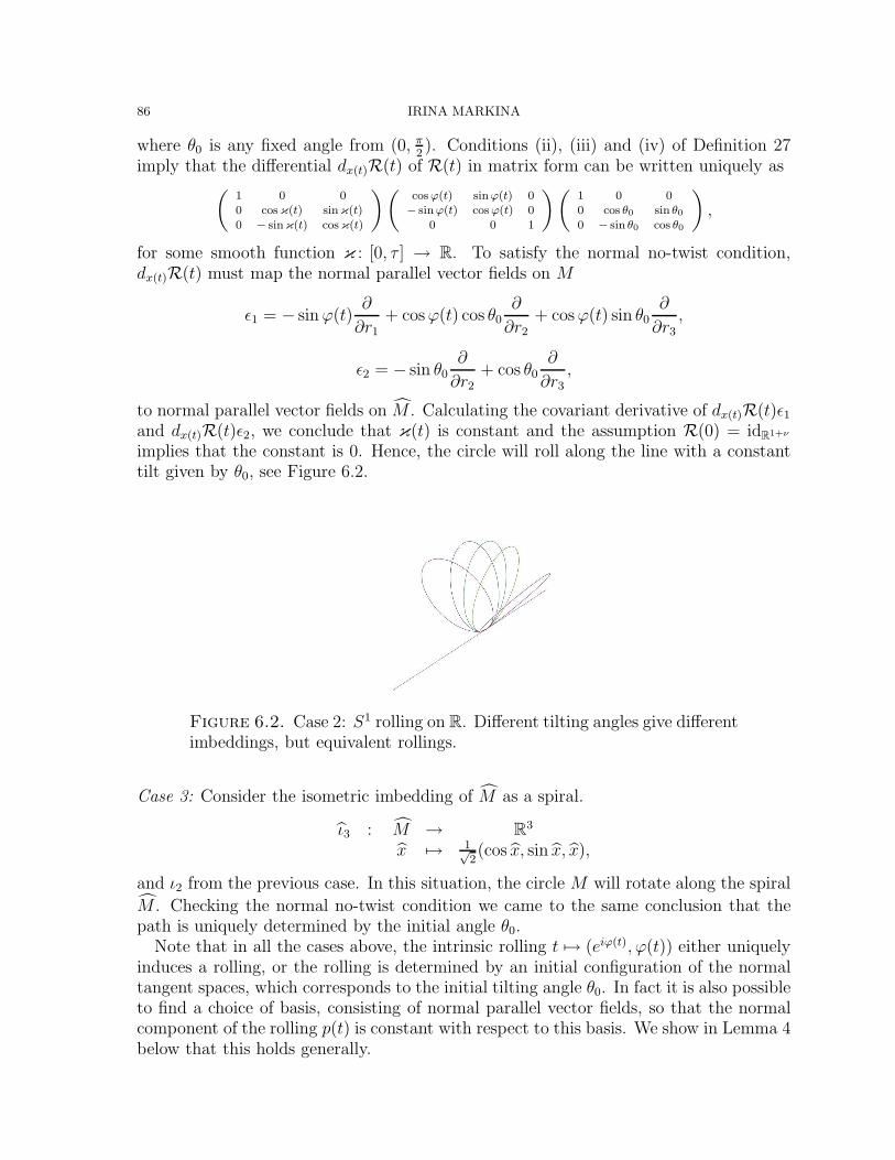
86 IRINA MARKINA
where θ0 is any fixed angle from (0, π2). Conditions (ii), (iii) and (iv) of Definition 27
imply that the differential dx(t)R(t) of R(t) in matrix form can be written uniquely as(1 0 00 cos κ(t) sin κ(t)
0 − sinκ(t) cos κ(t)
)(cosϕ(t) sinϕ(t) 0− sinϕ(t) cosϕ(t) 0
0 0 1
)(1 0 00 cos θ0 sin θ00 − sin θ0 cos θ0
),
for some smooth function κ : [0, τ ] → R. To satisfy the normal no-twist condition,dx(t)R(t) must map the normal parallel vector fields on M
ε1 = − sinϕ(t)∂
∂r1
+ cosϕ(t) cos θ0∂
∂r2
+ cosϕ(t) sin θ0∂
∂r3
,
ε2 = − sin θ0∂
∂r2+ cos θ0
∂
∂r3,
to normal parallel vector fields on M . Calculating the covariant derivative of dx(t)R(t)ε1and dx(t)R(t)ε2, we conclude that κ(t) is constant and the assumption R(0) = idR1+ν
implies that the constant is 0. Hence, the circle will roll along the line with a constanttilt given by θ0, see Figure 6.2.
Figure 6.2. Case 2: S1 rolling on R. Different tilting angles give differentimbeddings, but equivalent rollings.
Case 3: Consider the isometric imbedding of M as a spiral.
ι3 : M → R3
x %→ 1√2(cos x, sin x, x),
and ι2 from the previous case. In this situation, the circle M will rotate along the spiral
M . Checking the normal no-twist condition we came to the same conclusion that thepath is uniquely determined by the initial angle θ0.
Note that in all the cases above, the intrinsic rolling t %→ (eiϕ(t),ϕ(t)) either uniquelyinduces a rolling, or the rolling is determined by an initial configuration of the normaltangent spaces, which corresponds to the initial tilting angle θ0. In fact it is also possibleto find a choice of basis, consisting of normal parallel vector fields, so that the normalcomponent of the rolling p(t) is constant with respect to this basis. We show in Lemma 4below that this holds generally.
GEOMETRY WITH CONSTRAINTS 87
Let x : [0, τ ] → M and x : [0, τ ] → M be two fixed curves. We denote by ej(t)nj=1
a collection of parallel tangent vector fields along x(t) forming an orthonormal basis forTx(t)M and by ελ(t)νλ=1 a collection of normal parallel vector fields along x(t) formingan orthonormal basis for Tx(t)M
⊥. Such vector fields can be constructed by paralleltransport and normal parallel transport along x(t). Similarly, along x(t), we defineparallel frames ein
i=1 and εκνκ=1. Recall that Latin indices i, j, . . . vary from 1 to n,while Greek ones κ,λ, . . . vary from 1 to ν.
The following lemma shows that the image of a parallel frame over M has constant
coordinates in a parallel frame over M . This reflects the fact that rolling preservesparallel vector fields.
Lemma 4. A curve (q(t), p(t)) in Q ⊕ Pι,ι in the fibers over (x(t), x(t)), satisfies (II)and (III) if and only if the matrices
A(t) = (aij(t)) = (gM(ei, q(t)ej)), B(t) = (bκλ(t)) = (gM(εκ(t), p(t)ελ(t))),
are constant.
Proof. Check that the derivatives aij(t) and bij(t) vanish. !
The following theorem gives an answer to the first question raised at the beginning ofSubsection 6.2.3.
Theorem 6.1. [46] Let q : [0, τ ] → Q be a given intrinsic rolling map without slippingor twisting with projection prM×M q(t) = (x(t), x(t)). Define the vector spaces
V =v(t) is a parallel v. field along x(t), and gM(v(t), x(t)) = 0 for all t
,
V =v(t) is a parallel v. field along x(t), and gM(v(t), ˙x(t)) = 0 for all t
.
Then dim V = dim V and, if we denote this dimension by k, the following holds.
(a) The map q is the unique intrinsic rolling of M on M along x(t) and x(t) if andonly if k ≤ 1.
(b) If k ≥ 2, all the rollings along x(t) and x(t) differ from q by an element in
SO(V ).
In particular, if the curve x : [0, τ ] → M is a geodesic, we have the following conse-quence of Theorem 6.1.
Corollary 8. Assume that x(t) is a geodesic in M . Then there exists an intrinsic rolling
of M on M along (x(t), x(t)) if and only if x(t) is a geodesic with the same speed as x(t).
Moreover, if n ≥ 2, and if V is defined as in Theorem 6.1, then dim V = n− 1, and all
the rollings along x(t) and x(t) differ by an element in SO(V ).
Concerning the problem of extending intrinsic rollings to extrinsic ones, the followingtheorem gives a complete answer to the question posed at the beginning of Subsec-tion 6.2.3.
88 IRINA MARKINA
Theorem 6.2. Let q : [0, τ ] → Q be an intrinsic rolling and let ι : M → Rn+ν and
ι : M → Rn+ν be given imbeddings. Then, given an initial normal configuration
p0 ∈ (Pι,ι)(x0,x0), where (x0, x0) = prM×M q(0),
there exists a unique rolling (q, p) : [0, τ ] → Q⊕ Pι,ι satisfying p(0) = p0.
Proof. Let ελ(t)νλ=1 and εκ(t)νκ=1 be normal parallel frames along x(t) and x(t),respectively. Let B0 ∈ SO(ν) be defined by
B0 = (bκλ) = (〈εκ(0), p0 ελ(0)〉) .
Then p(t) must satisfy bκλ = 〈εκ(t), p(t) ελ(t)〉, by Lemma 4, and it is uniquely deter-mined by this. !
Analogously to the spaces V and V in Theorem 6.1, let us define the vector spaces
E = ε(t) is a normal parallel vector field along x(t) ,
E = ε(t) is a normal parallel vector field along x(t) ,
with inner product and orientation induced by TM⊥ and TM⊥. Both vector spaces havedimension ν. An extrinsic rolling (q, p) extending an intrinsic rolling q is determined up
to a left action of SO(E) or, equivalently, up to a right action of SO(E). Both SO(E)
and SO(E) are isomorphic to SO(ν), but not canonically.
6.3. Distributions for extrinsic and intrinsic rolling. The aim of this Subectionis to formulate the kinematic conditions of no-slipping and no-twisting in terms of adistribution. In this setting, a rolling will be a smooth curve almost everywhere tangentto this distribution.
6.3.1. Local trivializations of Q. Let π : Q ⊕ Pι,ι → M × M denote the canonicalprojection. Consider a rolling R(t) = (q(t), p(t)), then π R(t) = (x(t), x(t)). Given
an arbitrary t0 in the domain of R(t), let U and U denote neighborhoods of x(t0) and
x(t0) in M and M , respectively, such that both bundles TM and TM⊥ are trivialized
being restricted to U . In the same way we chose U , such that both TM and TM⊥ are
trivialized when they are restricted to U . This implies that the bundle
Q⊕ Pι,ι →M × M,
trivializes when it is restricted to U × U .Each of the requirements (I)-(III) can be written as restrictions to R(t). We will show,
that all admissible values of R(t) form a distribution; that is a smooth sub-bundle ofT (Q⊕ Pι,ι). We will use the local trivializations to describe this distribution.
GEOMETRY WITH CONSTRAINTS 89
6.3.2. The tangent space of SO(n). Let U and U be as in Subsection 6.3.1. Then weget in trivialization
Tπ−1(U × U) = TU × T U × TSO(n)× TSO(ν).
The decomposition requires that we present a detailed description of tangent spaces ofSO(n) and SO(ν) in terms of left and right invariant vector fields.
We start by considering the imbedding of SO(n) in GL(n). Denote the matrix entriesof a matrix A by (aij) and the transpose matrix by At. Then, differentiating the conditionAtA = 1, we obtain
TSO(n) =⋂i≤j
kerωij , ωij =n∑
r=1
(arj dari + ari darj) .
It is clear that the tangent space at the identity 1 of SO(n) is spanned by
Wij(1) :=∂
∂aij− ∂
∂aji, 1 ≤ i < j ≤ n.
We denote so(n) = spanWij(1) following the classical notation. We use left transla-tions of these vectors to define
(6.6) Wij(A) := dlAWij(1) =n∑
r=1
(ari
∂
∂arj
− arj∂
∂ari
)as global left invariant basis of TSO(n). Note that the left and right action in TSO(n)is described by
dlA( ∂
∂aij
)=
n∑r=1
ari∂
∂arj, drA
( ∂
∂aij
)=
n∑s=1
ajs∂
∂ais.
We have the following formula to switch from left to right translation and the other wayaround,
dlA( ∂
∂aij
)=
n∑r,s=1
ariasi
(drA
( ∂
∂ars
)), drA
( ∂
∂aij
)=
n∑r,s=1
ajsair
(dlA
( ∂
∂ars
)).
Therefore, the right invariant basis of TSO(n) can be written as
drA
(Wij(1)
)= AdA−1
(Wij(A)
)=∑r<s
(airajs − ajrais)Wrs(A).
If Wij is defined by (6.6) and i > j, (so Wij = −Wji) then the bracket relations aregiven by
[Wij , Wkl] = δj,kWil + δi,lWjk − δi,kWjl − δj,lWik.
90 IRINA MARKINA
6.3.3. Distributions. Now we are ready to rewrite the kinematic conditions (I)-(III) as adistribution. Let R(t) be a rolling satisfying the conditions (I)-(III). Consider it imageunder the trivializations. Then
(6.7) R(t) = x(t) + ˙x(t) +
n∑i,j=1
aij∂
∂aij+
ν∑κ,λ=1
bκλ∂
∂bκλ.
If we denote x(t) by Z(t), then (I) holds if and only if ˙x(t) = q(t)Z(t).We want to write the last two terms in (6.7) in the right invariant basis of correspond-
ing tangent spaces of SO(n) and SO(ν), based on conditions (II) and (III).Satisfying (II), we obtain
n∑i,j=1
aij∂
∂aij=∑i<j
(gM
(∇Z(t)q−1ej , q
−1ei
)− gM
(∇qZ(t)ej, ei
))AdA−1
(Wij(A)
).
Similarly, (III) holds if and only ifν∑
κ,λ=1
bκλ∂
∂bκλ=∑κ<λ
(g⊥M
(∇⊥Z(t)p−1ελ, p
−1εκ)− g⊥
M
(∇⊥qZ(t)ελ, εκ))
AdB−1
(Wκλ(B)
).
Here ej , ej, εκ, εκ, j = 1, . . . , n, κ = 1, . . . , ν, are orthonormal bases of correspondingtangent and normal spaces and gM , gM , g⊥M , g⊥
Mare restrictions of the Euclidean metric
on corresponding tangent and normal spaces of M and M .
Definition 30. If X is a vector field on M , then we define V(X) and V⊥(X) as thevector fields on Q⊕Pι,ι, such that under any local trivialization h and any (q, p) ∈ π−1(x)they satisfy
(6.8) dh (V(X)(q, p)) =∑i<j
(gM
(∇X(x)ej, ei
)− gM
(∇qX(x)qej , qei
))Wij(A).
(6.9) dh(V⊥(X)(q, p)
)=∑κ<λ
(g⊥M
(∇⊥X(x)ελ, εκ)− g⊥
M
(∇⊥qX(x)pελ, pεκ))
Wκλ(B).
Notice that if Y (x) = X(x) = X0 ∈ TxM , then V(Y )(q, p) = V(X)(q, p) for every(q, p) ∈ (Q⊕ Pι,ι)x. Hence, we may define V(X0)(q, p) whenever X0 ∈ TxM and (q, p) ∈(Q⊕ Pι,ι)x. Also notice that the map X %→ V(X) is linear. The same holds for V⊥.
At first glance, it may seem that all of the coefficients of Wij(A) and Wκλ(A) in (6.8)and (6.9) vanish from conditions (II) and (III), that is not true, however. Even though,for any tangential vector field X
D
dtX(x(t)) = ∇x(t)X(x(t)),
in general, ∇qx(t)q(t)ej does not coincide with Ddt
q(t)ej(x(t)). To see this, notice that
D
dtasj es(x(t)) = asj es(x(t)) + asj∇ ˙x(t)es(x(t)) = asj es(x(t)) + asj∇qx(t)es(x(t)),
while ∇qx(t)asj es(x(t)) = asj∇qx(t)es(x(t)). Similar relations hold for D⊥dt
.We sum up our considerations in this Section in the following result.
GEOMETRY WITH CONSTRAINTS 91
Proposition 10. A curve (q(t), p(t)) in Q⊕Pι,ι is a rolling if and only if it is a horizontalcurve with respect to the distribution E, defined by
E(q,p) =X0 + qX0 + V(X0)(q, p) + V⊥(X0)(q, p)|X0 ∈ TxM
,
where (q, p) ∈ (Q⊕ Pι,ι)x.
Using the same symbol to denote the restriction of V(X) to Q, we have
Proposition 11. A curve q(t) in Q is an intrinsic rolling if and only if it is a horizontalcurve with respect to the distribution D, defined by
Dq = X0 + qX0 + V(X0)(q)|X0 ∈ TxM , q ∈ Qx.
6.4. Examples of rollings and their controllability. In this section, we show twoexamples of rolling configurations, namely the sphere Sn rolling on Rn and the specialEuclidean group SE(3) rolling on its Lie algebra se(3). The first case is controllable,which follows from the fact that the distribution D, encoding rolling without slippingand twisting, is bracket generating and thus the Chow-Rashevskiı theorem holds. Thesecond example is not controllable, which follows from the orbit theorem and a strongversion of it for the case of analytic manifolds, see [3].
For the second example we study a particular intrinsic rolling, which we extend to anextrinsic rolling. This exemplifies the result obtained in Theorem 6.2.
A controllable example: Sn rolling on Rn We want to illustrate the prop-erties of the distribution D from Proposition 11, by proving that the unit sphere Sn
in Rn+1 rolling over Rn is a completely controllable system. This result was obtainedin [114] by different methods. The aim of this subsection is to show the controllabilityof the system directly from the Chow-Rashevskiı theorem.
Consider the unit sphere Sn as the submanifold of Rn+1,
Sn =
(x0, . . . , xn) ∈ Rn+1 |n∑
k=1
(xk)2 = 1
,
with the induced metric g. For an arbitrary point x = (x0, . . . , xn) ∈ Sn, at least one ofthe coordinates x0, . . . , xn does not vanish. Without loss of generality, we may assumethat xn .= 0, and consider the neighborhood
U = (x0, . . . , xn) ∈ Sn| ± xn > 0,where the choice of the ± sign depends on the sign of xn. To simplify the notation, wedefine the functions sj(x) =
∑nr=j(x
r)2 on U , for j = 1, . . . , n, that are strictly positiveon U . We use them to define an orthonormal basis of TU . Define the vector fields ej
on U
(6.10) ej =
√sj
sj−1
(− ∂
∂xj−1+
xj−1
sj
n∑r=j
xr ∂
∂xr
), j = 1, . . . , n.
These vector fields form an orthonormal basis of the tangent space over U and we denote
by Γkij the Christoffel symbols with respect to the basis ein
i=1. We set ei =∂
∂xito be
the standard basis of TRn. Let us state two technical lemmas whose proofs can beobtained by direct calculations or found in [46].
92 IRINA MARKINA
Lemma 5. Let 1 ≤ i < j ≤ n. Then Γikj = − xi−1
√si−1si
δk,j for all k = 1, . . . , n.
For convenience, we denote Γk = xk−1√
sk−1sk= −Γk
aa, a = 1, . . . , n. The properties of ∇have the following consequences:
• The compatibility of ∇ with the metric g and g(ei, ej) = δi,j , imply that Γikj = −Γj
ki.
In particular, Γiki = 0.
• The symmetry of ∇ implies that, if l < k, then
[ek, el] = ∇ekel −∇el
ek =n∑
i=1
g(∇ekel −∇el
ek, ei)ei = Γlek.
Lemma 6. We have
ek
(Γl)
=
0 , k > l,−1/sk , k = l,−Γl Γk , k < l.
k, l = 1, 2, . . . , n
Observe that ∇ekel = 0, and [ek, el] = 0 for all k, l = 1, . . . , n.
Consider the vector fields Xk = ek + qek + V(ek), restricted to U , which span thedistribution D introduced in Proposition 11. In this case, we have the explicit form
Xk(x, x, A) = ek(x) +
n∑i=1
aikei(x)−k−1∑i=1
Γi Wik(A).
In order to determine [Xk, Xl], we assume that k > l. Then
[Xk, Xl] = Γl Xk −Wlk.
Define the vector fields Ylk, for l < k, by Ylk := [Xl, Xk] + Γl Xk = Wlk. Finally, let
Z1 = [Y12, X2] =
n∑i=1
ai1ei, Zk = [X1, Y1k] =
n∑i=1
aikei , k = 2, . . . , n.
We conclude that the entire tangent space is spanned by the vector fields Xknk=1,
Ylk1≤l<k≤n and Zknk=1. Hence, D is a regular bracket generating distribution of step
3, which implies that the system of rolling Sn over Rn is completely controllable.
6.4.1. A non-controllable example: SE(3) rolling on R6. We consider the case of SE(3),endowed with a left invariant metric defined later, rolling over its tangent space at theidentity T1SE(3) = se(3), with metric obtained by restricting the left invariant metricon SE(3) to the identity. Our goal is to determine whether the system is controllable.
We give SE(3) coordinates as follows. For any x ∈ SE(3) there exist C = (cij) ∈SO(3) and r = (r1, r2, r3) ∈ R3, such that x = (C, r) acts on R3 via
x(y) = Cy + r, for all y ∈ R3.
The tangent space of SE(3) at x = (C, r) is spanned by the left invariant vector fields
e1 = Y1 =1√2
(C · ∂
∂c12− C · ∂
∂c21
)=
1√2
3∑j=1
(cj1
∂
∂cj2− cj2
∂
∂cj1
)
GEOMETRY WITH CONSTRAINTS 93
e2 = Y2 =1√2
(C · ∂
∂c13− C · ∂
∂c31
)=
1√2
3∑j=1
(cj1
∂
∂cj3− cj3
∂
∂cj1
)
e3 = Y3 =1√2
(C · ∂
∂c23− C · ∂
∂c32
)=
1√2
3∑j=1
(cj2
∂
∂cj3− cj3
∂
∂cj2
)
ek+3 = Xk = C · ∂
∂rk=
3∑j=1
cjk∂
∂rjk = 1, 2, 3.
Define a left invariant metric on SE(3) by declaring the vectors e1, . . . , e6 to form anorthonormal basis. The mapping
6∑j=1
xjej(1) %→ (x1, x2, x3, x4, x5, x6) ∈ R6
permits to identify se(3), endowed with the induced metric, with R6 endowed with theEuclidean metric. We write ek = ∂
∂xkon R6 and study the behavior of the intrinsic
rollings of SE(3) on R6. Note that the configuration space Q for intrinsic rolling isSE(3) × R6 × SO(6), because both manifolds SE(3) and R6 are Lie groups, so theirtangent bundles are trivial, and dim Q = 27.
The covariant derivatives ∇eiej are non-zero only in the following cases
∇Y1Y2 = − 1
2√
2Y3, ∇Y1Y3 =
1
2√
2Y2, ∇Y2Y3 = − 1
2√
2Y1,
∇Y1Xk =1√2
(δ2,kX1 − δ1,kX2) , ∇Y2Xk =1√2
(δ3,kX1 − δ1,kX3) ,
∇Y3Xk =1√2
(δ3,kX2 − δ2,kX3) ,
where δi,j denotes the Kronecker symbol. On the other hand, it is well-known that∇ei
ej = 0 for any i, j. Proposition 11 and Definition 30 show that the distribution Dover Q is spanned by
Z1 = Y1 + qY1 +1
2√
2W23 +
1√2W45, Z2 = Y2 + qY2 − 1
2√
2W13 +
1√2W46,
(6.11) Z3 = Y3 + qY3 +1
2√
2W12 +
1√2W56,
K1 = X1 + qX1, K2 = X2 + qX2, K3 = X3 + qX3.
In the case of D, defined by the vector fields (6.11) straightforward calculations yieldthat the flag associated to D is on the form
(6.12)D2 = D ⊕ span W12, W13, W23,D3 = D2 ⊕ spanqY1, qY2, qY3,D4 = D3,
and so dim D2 = 9, dim Dk = 12 for all k ≥ 3 and the step of D is 3.
94 IRINA MARKINA
It follows from (6.12) that the distribution is not bracket generating and we can notproduce all the tangent space to the configuration space, that has dimension 27 at eachpoint. We conclude that the system is not controllable by orbit theorem [3].
6.4.2. Concrete example of an intrinsic rolling. . We end this section with a concreteexample of an intrinsic rolling q(t) = (x(t), x(t), A(t)), where
x(0) = idR3, x(0) = 0, A(0) = 1.
Define the curve x : [0, τ ] → SE(3) by
(6.13) x(t)y =
cos θ(t) sin θ(t) 0− sin θ(t) cos θ(t) 0
0 0 1
y1
y2
y3
+
00
ψ(t)
, y ∈ R3,
where θ(t) and ψ(t) are smooth functions with θ(0) = ψ(0) = 0. Then x =√
2 θ(t)Y1 +
ψ(t)X3 for every t, and the intrinsic rolling has the form q =√
2 θ(t)Z1 + ψ(t)K3. Thisimplies that
(6.14) ˙x(t) =√
2 θ(t) qY1 + ψ(t) qX3, A(t) = θ(t)
(1
2W23(A) + W45(A)
)for almost every t. It follows from the first equation in (6.14) that
x(t) =(√
2 θ(t), 0, 0, 0, 0,ψ(t))tr
,
where tr denotes transposition. By exponentiating the second equation in (6.14), weobtain
A(t) =
1 0 0 0 0 0
0 cos(
θ(t)2
)sin
(θ(t)2
)0 0 0
0 − sin(
θ(t)2
)cos
(θ(t)2
)0 0 0
0 0 0 cos θ(t) sin θ(t) 00 0 0 − sin θ(t) cos θ(t) 00 0 0 0 0 1
.
Imbedding of SE(n) into Euclidean space. Since it is less obvious how toextend an intrinsic rolling of SE(3) on se(3) to an extrinsic rolling in ambient space, wedescribe an isometric imbedding of SE(n) into the Euclidean space R(n+1)2 . Identify an
element C ∈ R(n+1)2 with the matrix
C =
c11 · · · c1,n+1...
. . ....
cn+1,1 · · · cn+1,n+1
.
Define the inner product on R(n+1)2 by⟨C1, C2
⟩= trace
((C1
)tC2
). Note that since⟨
C, C⟩
=∑n+1
i,j=1 |cij |2, the metric 〈·, ·〉 coincides with the Euclidean metric. From this
we get that
∂∂cij
n+1
i,j=1is an orthonormal basis for the tangent bundle TR(n+1)2 with
respect to 〈·, ·〉.
GEOMETRY WITH CONSTRAINTS 95
We define the imbedding of SE(3) into R(n+1)2 by
ι : SE(n) → R(n+1)2
x = (C, r) %→ C =
(C r0 1
).
This mapping is in fact an isometry of SE(n) onto its image. To see this, notice that the
metrics coincide at the identity, and that the metric of R(n+1)2 , restricted to the imageIm(ι) of ι, is left invariant under the action of SE(n). Hence, the metrics on SE(n) andIm(ι) coincide, and ι defines an isometric imbedding.
Extrinsic rolling of SE(3) over se(3). We will use the constructed imbeddingto build an extrinsic rolling of SE(3) over se(3) in R16 and we write M for the image ofSE(3) in R16 under this imbedding. Denote ∂ij = ∂
∂cij, then the vector fields spanning
TM are
e1 = Y1 =1√2
3∑i=1
(ci1∂i2 − ci2∂i1) , e2 = Y2 =1√2
3∑i=1
(ci1∂i3 − ci3∂i1) ,
(6.15) e3 = Y3 =1√2
3∑i=1
(ci2∂i3 − ci3∂i2) , e3+k = Xk =3∑
j=1
cik∂i4, k = 1, 2, 3,
where we suppressed dι in the notation. We introduce an othonormal basis of TM⊥
Υ1 =1√2
3∑j=1
(cj1∂j2 + cj2∂j1) , Υ2 =1√2
3∑j=1
(cj1∂j3 + cj3∂j1) ,
Υ3 =1√2
3∑j=1
(cj2∂j3 + cj3∂j2) ,
(6.16) Ψλ =
3∑j=1
cjλ∂jλ, λ = 1, 2, 3, Ξµ = ∂4µ, µ = 1, 2, 3, 4.
We denote by M the image of R6 into R16 by the imbedding
(x1, x2, x3, x4, x5, x6)ι%→
0 1√
2x1
1√2x2 x4
− 1√2x1 0 1√
2x3 x5
− 1√2x2 − 1√
2x3 0 x6
0 0 0 0
.
We have the following orthonormal basis of TM ,
e1 =1√2(∂12 − ∂21), e2 =
1√2(∂13 − ∂31), e3 =
1√2(∂23 − ∂32),
e3+k = ∂k4, k = 1, 2, 3,
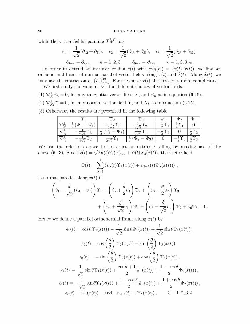
96 IRINA MARKINA
while the vector fields spanning TM⊥ are
ε1 =1√2(∂12 + ∂21), ε2 =
1√2(∂13 + ∂31), ε3 =
1√2(∂23 + ∂32),
ε3+κ = ∂κκ, κ = 1, 2, 3, ε6+κ = ∂4κ, κ = 1, 2, 3, 4.
In order to extend an intrinsic rolling q(t) with π(q(t)) = (x(t), x(t)), we find anorthonormal frame of normal parallel vector fields along x(t) and x(t). Along x(t), we
may use the restriction of εκ10κ=1. For the curve x(t) the answer is more complicated.
We first study the value of ∇⊥ for different choices of vector fields.
(1) ∇⊥XΞµ = 0, for any tangential vector field X , and Ξµ as in equation (6.16).
(2) ∇⊥XkΥ = 0, for any normal vector field Υ, and Xk as in equation (6.15).
(3) Otherwise, the results are presented in the following table
Υ1 Υ2 Υ3 Ψ1 Ψ2 Ψ3
∇⊥Y1
12(Ψ1 −Ψ2) − 1
2√
2Υ3
12√
2Υ2 −1
2Υ1
12Υ1 0
∇⊥Y2− 1
2√
2Υ3
12(Ψ1 −Ψ3)
12√
2Υ1 −1
2Υ2 0 1
2Υ2
∇⊥Y3− 1
2√
2Υ2
12√
2Υ1
12(Ψ2 −Ψ3) 0 −1
2Υ3
12Υ3
.
We use the relations above to construct an extrinsic rolling by making use of thecurve (6.13). Since x(t) =
√2 θ(t)Y1(x(t)) + ψ(t)X3(x(t)), the vector field
Ψ(t) =
3∑λ=1
(υλ(t)Υλ(x(t)) + υ3+λ(t)Ψλ(x(t))) ,
is normal parallel along x(t) if(υ1 − θ√
2(υ4 − υ5)
)Υ1 +
(υ2 +
θ
2υ3
)Υ2 +
(υ3 − θ
2υ2
)Υ3
+
(υ4 +
θ√2υ1
)Ψ1 +
(υ5 − θ√
2υ1
)Ψ2 + υ6Ψ3 = 0.
Hence we define a parallel orthonormal frame along x(t) by
ε1(t) = cos θΥ1(x(t))− 1√2
sin θΨ1(x(t)) +1√2
sin θΨ2(x(t)) ,
ε2(t) = cos
(θ
2
)Υ2(x(t)) + sin
(θ
2
)Υ3(x(t)) ,
ε3(t) = − sin
(θ
2
)Υ2(x(t)) + cos
(θ
2
)Υ3(x(t)) ,
ε4(t) =1√2
sin θΥ1(x(t)) +cos θ + 1
2Ψ1(x(t)) +
1− cos θ
2Ψ2(x(t)) ,
ε5(t) = − 1√2
sin θΥ1(x(t)) +1− cos θ
2Ψ1(x(t)) +
1 + cos θ
2Ψ2(x(t)) ,
ε6(t) = Ψ3(x(t)) and ε6+λ(t) = Ξλ(x(t)) , λ = 1, 2, 3, 4.
GEOMETRY WITH CONSTRAINTS 97
Thus p(t) is represented by a constant matrix in the bases ελ(t)10λ=1 and εκ(t)10
κ=1.Let us choose p(t) to be the identity in these bases, due to the given imbedding.
The curve R(t) = (q(t), p(t)) in SE(16) is given by R(t)(t)x = Ax + r(t), where
A(t) =
cos2 θ2
− sin θ2
0 0 sin θ2
cos θ−12
0 0 0 0sin θ
2cos2 θ
20 0 sin2 θ
2sin θ
20 0 0 0
0 0 cos θ2
0 0 0 sin θ2
0 0 0
0 0 0 1 0 0 0 0 0 0
− sin θ2
sin2 θ2
0 0 cos2 θ2
− sin θ2
0 0 0 0 010×6cos θ−1
2− sin θ
20 0 sin θ
2cos2 θ
20 0 0 0
0 0 − sin θ2
0 0 0 cos θ2
0 0 0
0 0 0 0 0 0 0 1 0 0
0 0 0 0 0 0 0 0 cos θ2
− sin θ2
0 0 0 0 0 0 0 0 sin θ2
cos θ2
06×10 16
,
and r(t) =
(−1,
θ√2, 0, 0,
θ√2,−1, 0, 0, 0, 0,−1, 0, 0, 0, 0, 0
)t
. Here, 0m×n denotes the
zero matrix of size m× n and 16 is the identity matrix of size 6× 6.
7. Group of diffeomorphisms of the circle
In this section we consider one of the simplest examples of an infinite dimensionalmanifold posessing rather good structure and having various applications. We startfrom the definitions, then we give motivations and we finish with some results concerningsub-Riemannian structure of this example. The material of this section can be foundin [64, 76, 82, 91, 98].
7.1. Manifold and group structure of Diff S1. Let S1 be the unit circle with thestandard counterclockwise orientation that we will think of as R mod 2πZ. Denote byDiff S1 the set of all C∞-diffeomorphisms of S1 preserving the orientation. This is anopen subset of the infinite dimensional space C∞(S1, S1) of all C∞-smooth maps of thecircle, see Exercise 1. The topology defined on the space C∞(S1, S1) is C∞ topology,which corresponds to the uniform convergence of all derivatives of h ∈ C∞(S1, S1) andit can be described by the countable system of semi-norms
‖h‖m = supθ∈S1
|hm(θ)|.
The set Diff S1, considered as an open set of C∞(S1, S1), inherits C∞-topology.Define the group operation in Diff S1 as the composition of two diffeomorphisms and
the inverse element of the group as the inverse map. The identity map id: S1 → S1
becomes the unit of the group. We would like to consider the defined group as an infinitedimensional analogue of a Lie group. To do this we need to define a manifold structure onthe topological space Diff S1. We start from the choice of a model vector space V, wherethe coordinate charts (U,ϕ) with U being an open set on Diff S1 and ϕ : U → V ⊂ Vbeing a diffeomorphism, will be constructed. The space Vect S1 of all C∞ real vectorfields on the circle is a good candidate for the model space V since it possesses the Frechettopology and it is one of the examples of a locally convex topological vector space. Thevector fields S1 $ θ → v(θ) d
dθ= v(θ)∂θ ∈ Vect(S1) can be associated with the space
98 IRINA MARKINA
C∞(S1, R) of real functions v. A sketch of the construction of the chart is given below.Let us consider a neighborhood V0 of 0 ∈ Vect S1: V0 = v ∈ Vect(S1) | ‖v‖ ≤ π.Then there is a homeomorphic map ψ : V0 → U0 ⊂ C∞(S1, S1) to a neighborhood
U0 = f ∈ C∞(S1, S1) | f(θ) .= −θ, for all θ ∈ S1,of the identity map id ∈ C∞(S1, S1). Construction of ψ see in Exercise 2. Choose anopen set U ⊂ U0 consisting of diffeomorphisms. Then U is a neighborhood of id ∈Diff S1. Then the set V = ψ−1(U) will be an open subset of V0 ∈ Vect(S1). Thus,we constructed the chart (U,ϕ), ϕ = ψ−1|U in a neighborhood of the identity mapid ∈ Diff S1. To construct a complete atlas we exploit the group structure of Diff S1. IfU is a neighborhood of id ∈ Diff S1, then f.U = φ ∈ Diff S1 | φ = f h, h ∈ U is aneighborhood of f . Having the map ψ, we define ψf : V → f.U for any f ∈ Diff S1 asthe composition f ψ. Then the chart (Uf ,ϕf), where Uf = f.U and ϕf = ψ−1
f |f.U is
the corresponding local chart about any group element f ∈ Diff S1. The reader has toverify that any composition ϕhϕ
−1f is a smooth map in Vect(S1).
As we know, the space Vect(S1) endowed with usual brackets for vector fields forms aLie algebra, that we shall denote by the same symbol Vect(S1). On the other hand, thespace Tid Diff S1 furnished with brackets for tangent vectors is the Lie algebra diffS1.As we discussed in Subsection 2.1, a tangent vector is the equivalence class of all curvesf : R → Diff S1 such that f(0) = id and that have the same initial velocity. Such curvescan be seen as smooth functions
f : R× S1 → S1, f(0, θ) = θ,
where f(t0, θ) ∈ Diff S1 for any fixed value t0 ∈ R. The velocity vector at t = 0,corresponding to the equivalence class [f ], is a vector field
v(θ) =∂
∂t
∣∣∣t=0
f(t, θ), f ∈ [f ],
defined on S1. By this we identify Vect(S1) and diffS1 with the Lie product [X, Y ] =Y X−XY . Now we explain why the sign in the latter commutation relation is opposite.The action of the group Diff S1 on the circle S1, considered as a smooth compact orientedmanifold, is defined as the natural left action
µ : Diff S1 × S1 → S1
f.θ %→ f(θ).
The differential dµ acts at the level of tangent spaces: dµ : T (Diff S1×S1) ∼= T Diff S1×TS1 → S1. In order for the following diagram to commute
T (Diff S1 × S1) $ w(f, θ)dµ
!! v(f(θ)) ∈ TS1
Diff S1 × S1 $ (f, θ)
((
µ!! f(θ) ∈ S1
((
or dµ(w(f, θ)) = v(µ(f, θ)) = v(f(θ)) we have to extend the elements of diff as right
invariant vector fields on Diff S1, or w(f, ·) = ddε
∣∣∣ε=0
(exp εw0)f(·), where w0 ∈ diff =
Tid Diff S1 ∼= Vect(S1) and the exponential map is defined in (7.1). In this way we
GEOMETRY WITH CONSTRAINTS 99
associate the elements of diff with right invariant vector fields. The brackets in diff isdefined as in Vect(S1), but with the opposite sign, see the discussion in Subsection 3.1.Thus
diff =(
Vect(S1), [ , ])
with [u∂θ, v∂θ] = (−uv′ + u′v)∂θ.
The group exponential map is defined in a standard way through one parametricsubgroup in Diff S1. The one parametric subgroup R $ t %→ f(t, θ) ∈ Diff S1 of diffeo-morphisms for any fixed value θ0 ∈ S1 is the solution of the Cauchy problem
dθdt
= v(θ) ∈ TθS1, where v(θ) = ∂
∂t
∣∣∣t=0
f(t, θ)
θ(0) = θ0.
Thus, the solution θ(t) = expθ0(tv) is the exponential curve that carries each line t %→ tvthrough the origin in Vect(S1) to the one parametric subgroup in Diff(S1) and
(7.1)exp : Vect(S1) → Diff(S1)
v %→ exp(v)
is the Diff S1-group exponential map.The interesting feature is that, in contrast to finite dimensional groups, there is no
neighborhood of id ∈ Diff S1, where the exponential map would be diffeomorphism. Themap is not locally surjective. No matter how small the neighborhood U of the identitymap id ∈ Diff S1, there is f ∈ U such that f does not belong to any one-parametricsubgroup, or f /∈ Im(exp), see Exercise 3.
Moreover, the map exp is not injective. Let fn be a rotation by the angle 2πn
: θfn%→
θ+ 2πn
. The map fn belongs to the closed subgroup S1 ⊂ Diff(S1) of rotations in Diff S1.Any one-parameter element of S1 is generated by a constant vector field v in (7.1). Let
H = φ ∈ Diff(S1) | φ(θ +
2π
n
)= φ(θ) +
2π
n
be the subgroup of Diff S1 of all periodic diffeomorphisms with period 2πn
. It easy to seethat fn commutes with H. Then since
S1 $ fn = φfnφ−1 ∈ φS1φ−1, φ ∈ H,
we conclude that fn belongs to all one-parametric subgroups from φS1φ−1, φ ∈ H.Finally, we state a property of the group Diff S1 and its Lie algebra Vect S1 whose
proof can be found in [55].
Proposition 12. The group Diff S1 is a simple group.
For practical purposes it is convenient to introduce a basis of Vect(S1). Since weidentify the vector fields v(θ)∂θ with smooth functions v(θ) on S1 and the latter canbe developed into the Fourier series, therefore, the Fourier basis cos(nθ), sin(nθ), n =0, 1, . . . is a natural choice of a basis for Vect(S1).
We observe also that all f ∈ Diff S1 are periodic functions with the period 2π in thefollowing sense
f(θ + 2π) = f(θ) + 2π.
Exercises
100 IRINA MARKINA
1. Define
η(f) = infθ,ϑ∈S1,θ -=ϑ
‖f(θ)− f(ϑ)‖‖θ − ϑ‖ , where f : S1 → S1, f ∈ C∞(S1).
Here ‖ · ‖ means the Euclidean distance in R2. Verify that η is a continuousfunction of f . Conclude that since η(f) > 0 if and only if f is a diffeomorphism,the set Diff S1 is an open set in C∞(S1, S1).
2. Let
V0 = v ∈ Vect(S1) | ‖v‖ ≤ π,and
U0 = f ∈ C∞(S1, S1) | f(θ) .= −θ, ∀ z ∈ S1be neighborhoods of 0 ∈ Vect(S1) and the identity map id ∈ C∞(S1, S1), re-spectively. We construct a map ψ : V0 → U0 by the following. Define a mapψv : S1 → S1 for v ∈ V0 as a map that sends a point θ ∈ S1 to the end point ofthe arc of length ‖v‖, which starts at θ with the initial velocity v(θ). Show thatψ is the homeomorphism from V0 $ v → ψv ∈ U0.
3. Let n ∈ N be big enough, and ε ∈ (0, 1n). We think of S1 = θ ∈ R mod 2πZ.
Consider the diffeomorphism
f(θ) = θ +π
n+ ε sin2(nθ).
Show that by choosing n and ε we can make f(θ) so close in C∞-topology to theidentity map as we want. Show that f has only one periodic orbit of period 2n.(Hint: start from θ = 0.) Show that starting from any other value θ ∈ (0, π/n) weget a non-periodic orbit. Conclude that f cannot belong to any one-parametersubgroup of Diff S1. Indeed if it belonged to exp(v) for some v ∈ Vect(S1),then it would be a rotation f(θ) = θ + π
n, since after 2n repetitions we get
[f(0)]2n = 2π = f(0 + 2π). But we know that it is not true since all other pointsof S1 do not belong to the same orbit of f . See also [64, 91, 98].
4. Calculate the commutator in Vect(S1) for its basis cos(nθ), sin(nθ), n = 0, 1, . . ..
7.1.1. Central extensions of Diff S1 and Vect(S1). To introduce the central extensionsof the Lie-Frechet group Diff S1 and it Lie algebra Vect(S1) we start from the linearobject, i. e. from the Lie algebra.
Definition 31. The central extension g of a Lie algebra g by the Lie algebra R of realnumbers is the set g×R and new Lie brackets [(ξ, a)(η, b)]g, ξ, η ∈ g, a, b ∈ R, satisfyingthe axioms of Definition 50.
In this case R becomes the center of the extended Lie algebra. The simplest trivialexample of a central extension is the direct product g×R with the Lie brackets definedby
[(ξ, a)(η, b)]g := ([ξ, η]g, ab− ba) = ([ξ, η]g, 0).
We are interested in a non-trivial extension. In order to get it we need to find aninvariant skew symmetric bi-linear form ω : g × g → R, such that new Lie brackets
GEOMETRY WITH CONSTRAINTS 101
[(ξ, a)(η, b)]g := ([ξ, η]g,ω(ξ, η)) in the extended Lie algebra g satisfies the axioms ofDefinition 50. It leads to the condition on ω, which is called cocycle condition:
(7.2) ω([ξ, η], ζ) + ω([η, ζ ], ξ) + ω([ζ , ξ], η) = 0.
The form ω is called a 2-cocycle, and the terminology comes from the cohomology theory.It was shown in [44] that there is an essentially unique non-trivial 2-cocycle for the Liealgebra Vect(S1), which is called the Gelfand-Fuchs Lie algebra cocycle. It is given bythe following form ω.
ω(u(θ)∂θ, v(θ)∂θ
)=
1
2π
∫S1
u′(θ)v′′(θ) dθ =1
2π
∫S1
u′(θ)dv′
=1
4π
∫S1
det
(u′(θ) v′(θ)u′′(θ) v′′(θ)
)dθ.(7.3)
The central extension of the Lie algebra Vect(S1) by R is called the Virasoro algebra,is denoted by vir and it is unique up to an isomorphism. The name of the algebra iscoming from the name of the Argentinian physicist Miguel Angel Virasoro, who inventedthe idea of central extension for Vect S1 in his physical calculations. In physics, actually,more general 2-cocycle is used. Let us explain the mathematical background of thismore general 2-cocycle.
Definition 32. A 2-cocycle ω : g → R is called a 2-coboundary if there exists a linearmap η : g → R such that ω(ξ, υ) = η([ξ, υ]) for all ξ, υ ∈ g.
Let us assume that the central extension of g is given by a 2-coboundary η, e. g. (ξ, a) ∈g and [(ξ, a), (υ, b)] = ([ξ, υ], η([ξ, υ])). Then the change of the variables (ξ, a) %→ (ξ, a−η(x)) leads to
([ξ, υ], η([ξ, υ])) %→ ([ξ, υ], 0).
We again obtained the trivial extension. By this observation, in describing different cen-tral extensions one is interested only in the 2-cocycles modulo 2-coboundaries. Mean-while, in physical applications the following general form of 2-cocycle ωh,c for somepositive constants h, c is used:
(7.4) ωh,c
(u(θ)∂θ, v(θ)∂θ
)=
1
2π
∫S1
((h− c
12
)v′(θ)− c
12v′′′(θ)
)u dθ.
The constant c received the name central charge in physics and its value depends on theunderlying physical theory. The cocycle ω from (7.3) is obtained by setting h = c
12up
to the normalization factor c12
and is often called the classical Gelfand-Fuchs 2-cocycle.The following question arises: is there a group, whose Lie algebra is vir? The answeris positive. The corresponding group is called the Virasoro-Bott group and is denotedby Vir. The Virasoro-Bott group is topologically a direct product of Diff S1 and R:Vir = Diff S1 × R. In this case the multiplication in Vir can be defined as follows
(7.5) (f, a)(h, b) = (f h, a + b + λ(f, h)), f, g ∈ Diff S1, a, b ∈ R,
where λ : Diff S1 × Diff S1 → R is a smooth function that makes the multiplicationlaw (7.5) associative. The associativity of (7.5) corresponds to the group cocycle identity:
(7.6) λ(f h, g) + λ(f, h) = λ(f, h g) + λ(h, g).
102 IRINA MARKINA
The infinitesimal version of the Lie group 2-cocycle is the Lie algebra 2-cocycle. Thefollowing theorem gives the group 2-cocycle for the classical Gelfand-Fuchs 2-cocycleand was obtained for the first time in [15].
Proposition 13. The map
B : Diff S1 × Diff S1 → S1
(f, h) %→ 14π
∫S1 log(f h)′ d log h′
is a continuos 2-cocycle on the group Diff S1. Here f, h ∈ Diff S1 and f ′, h′ are theirderivatives with respect to θ ∈ S1.
Proof. For the proof we need to verify the group 2-cocycle condition (7.6) and thento check that the infinitesimal version coincides with the classical Gelfand-Fuchs 2-cocycle ω. The details can be found in [64]. !
As in the case of the central extension of a Lie algebra, any central extension of a Liegroup is defined up to a 2-coboundary.
Definition 33. A smooth 2-cocycle λ : G → R is called a 2-coboundary (on G) if thereexists a smooth map F : G → R such that
λ(f, h) = F (f) + F (g)− F (f g).
Two group 2-cocycles define isomorphic extensions if they differ by a 2-coboundary.Let us construct a group 2-coboundary for the group Diff S1. First, we write the generalLie algebra cocycle ωh,c in the following form
ωh,c
(u(θ)∂θ, v(θ)∂θ
)=
1
2π
∫S1
((h− c
12
)v′(θ)− c
12v′′′(θ)
)u dθ
=1
2π
∫ 2π
0
(αuv′ + βu′v′′
)dθ =: αa + βb,
where α = h − c12
, β = c12
and we used integration by parts of periodic functions u
and v on S1. Let us verify that a(u, v) = 12π
∫ π
0uv′ dθ is the Lie algebra 2-coboundary.
Introduce the functional
η(u∂θ) =1
2π
∫ 2π
0
u(θ) dθ,
expressing the mean value of u on S1. Observe that
η([u, v]) =1
2π
∫ 2π
0
u′(θ)v(θ)− v′(θ)u(θ) dθ = −21
2π
∫ 2π
0
u(θ)v′(θ) dθ = −2a(u, v)
by integration by parts. Thus a is a group 2-coboundary. The part b(u, v) = 12π
∫ π
0u′v′′ dθ
is the Gelfand-Fuchs algebra 2-cocycle. The multiplication law (7.5) takes the form
(f, a)(h, b) = (f h, a + b + αA(f, h) + βB(f, h)), f, g ∈ Diff S1, a, b ∈ R.
Here B(f, h) is the Bott 2-cocycle given by Proposition 13 and A(f, h) is the group2-coboundary satisfying Definition 33. To find the smooth function F we verify thefollowing two properties.
1. Since the identity element on Vir has the form (id, 0) we get A(f, id) = 0 =⇒F (id) = 0, id ∈ Diff S1 by the multiplication law (7.5).
GEOMETRY WITH CONSTRAINTS 103
2. In order for the inverse element to (f, a) ∈ Vir to take the form (f−1,−a) werequire A(f, f−1) = 0 =⇒ F (f) + F (f−1) = 0.
The function F (f) =∫ 2π
0
(f(θ)−θ
)dθ obviously satisfies the first property. Let us show
that it also satisfies the second property.Step 1. First we assume that f(0) = 0. Then f(2π) = 2π and f is strictly increasing
on [0, 2π]. Thus
F (f) + F (f−1) =
∫ 2π
0
(f(θ) + f−1(θ)− 2θ
)dθ
=
∫ 2π
0
∫ f
0
dθdy +
∫ 2π
0
∫ 2π
f
dθdy − 4π2 = 0.
Step 2. Now we assume that f is an arbitrary element of Diff S1. Define f(θ) =
f(θ + f−1(0)). Then f(θ) satisfies
a) f(0) = 0,
b) f−1(θ) = f−1(θ)− f−1(0),
c)∫ 2π
0f(θ + s) dθ =
∫ 2π
0
(f(θ) + s
)dθ for any s ∈ R.
Indeed, the properties a), b) are obvious and to show c) we observe that f(θ) − θ is a
periodic function with the period 2π by f(θ + 2πk) = f + 2πk, k ∈ N. Then∫ 2π
0
f(θ + s) dθ =
∫ 2π+s
s
f(θ)− θ dθ +
∫ 2π+s
s
θ dθ
=
∫ 2π
0
f(θ)− θ dθ +1
2
((2π + s)2 − s2
)=
∫ 2π
0
f(θ) dθ + 2πs =
∫ 2π
0
(f(θ) + s
)dθ.
We continue to prove the second property for an arbitrary f ∈ Diff S1 and deduce
F (f) + F (f−1) =
∫ 2π
0
(f(θ) + f−1(θ)− 2θ
)dθ
=
∫ 2π
0
(f(θ − f−1(0)
)+ f−1(θ) + f−1(0)− 2θ
)dθ
=
∫ 2π
0
(f(θ)− f−1(0) + f−1(θ) + f−1(0)− 2θ
)dθ
= F (f) + F (f−1) = 0
by the Step 1 and a), b), c).We conclude, that
(7.7) A(f, h) =
∫ 2π
0
(f(θ) + h(θ)− f h(θ)− θ
)dθ.
The last step in defining group 2-coboundary A is to verify that the infinitesimalversion of A from (7.7) coincides with the algebra 2-coboundary a. We will use thefollowing.
104 IRINA MARKINA
Proposition 14. [64] Let A : G × G → R be a group 2-cocycle defining a centralextension by R of the group G. Then the algebra 2-cocycle a : g × g → R defining thecorresponding central extension of the Lie algebra g of G is given by
a(u, v) =d2
dtds
∣∣∣t=0,s=0
A(ft, hs)− d2
dtds
∣∣∣t=0,s=0
A(hs, ft),
where ft and hs are smooth curves in G such that
d
dt
∣∣∣t=0
ft = u,d
ds
∣∣∣s=0
hs = v.
Now, differentiating (7.7) we obtain∫ 2π
0
(− ∂
∂θ∂∂t
ft∂∂s
hs + ∂∂θ
∂∂s
hs∂∂t
ft
)dθ∣∣∣t=0,s=0
=∫ 2π
0
(− v∂θu + u∂θv)dθ = −2πη([u, v]) = 4πa(u, v).
Normalizing the 2-coboundary (7.7), we finally deduce
A(f, h) =1
4π
∫ 2π
0
(f(θ) + h(θ)− f h(θ)− θ
)dθ.
Example 9. Here we present the Heisenberg algebra from the central extension pointof view. Take the abelian Lie algebra g = R2 and an arbitrary skew symmetric bilinearform ω : R2 × R2 → R. Since the Lie algebra g is Abelian, the 2-cocycle condition (7.2)is trivial and the form ω satisfies it. The resulting central extension of R2 by R is theset h = R2 ⊕ R endowed with the brackets
[h1, h2] = [(v1, r1), (v2, r2)] = [(0,ω(v1, v2))].
Note that the choice of any other skew-symmetric bilinear form leads to an isomorphic
Lie algebra h. The Lie algebra h with a non-degenerate form ω is a representative ofthis isomorphism class and it is called the three-dimensional Heisenberg algebra.
The n-dimensional analogue can be obtained by taking g = R2n+1 and an arbitraryskew symmetric bilinear form ω : R2n+1 × R2n+1 → R.
We even can continue and present an infinite dimensional version of the Heisenbergalgebra as a central extension of the space
g = f ∈ C(S1, S1) | η(f) =1
2π
∫S1
f(θ) dθ = 0.The space g is considered as an abelian algebra. Since a function with vanishing meanvalue can be written as a Fourier series
f(θ) =
∞∑n=1
xn cos(nθ) + yn sin(nθ),
it can be interpreted as a point in an infinite dimensional space. The 2-cocycle ω : g×g →R is given by
(7.8) ω(f, g) =
∫S1
f ′(θ)g(θ) dθ.
Exercises
GEOMETRY WITH CONSTRAINTS 105
1. Prove the cocycle condition (7.2) for the Gelfand-Fuchs cocycle (7.3).2. Calculate the Heisenberg group 2-cocycle that corresponds to the algebra 2-
cocycle (7.8).
7.1.2. Complexification of Vect(S1) and the Virasoro algebra. The next step is to con-sider complexifications of Vect(S1) and vir and their relations to Diff S1 and Vir. Thereader who is not familiar with the general construction of complexification can find allthe necessary definitions in Appendix A, Subsection 8.4.
The complexification Vect(S1) ⊗ C consists of smooth complex-valued vector fieldsv(θ)∂θ defined on S1, that can be identified with the space C∞(S1, C). The naturalbasis is the complex valued Fourier basis ek := −ieikθ∂θ, k ∈ Z, produced from the realFourier basis. The commutation relations for basic vector fields on Vect(S1)⊗ C are
[em, en] = (n−m)em+n, m, n ∈ Z.
These relations are known under the name of Witt, and the Lie algebra whose basissatisfies the Witt relations is called the Witt algebra. So the complexification of theLie algebra Vect(S1) is the Witt algebra. Actually, the complex valued vector fieldsek = −ieikθ∂θ can be extended to meromorphic vector fields Lk = zk+1 d
dzon C ∪ ∞,
that are holomorphic vector fields in C \ 0. The extended to the Riemann sphereC = C ∪ ∞ algebra of complex valued vector fields zk+1 d
dz∞k=−∞ is also called the
Witt algebra.The complexification of the Lie algebra Vect(S1) does not correspond to any Lie
group. The explanation can be the following. First, we observe that the Lie algebraVect(S1) contains Lie sub-algebras gk = span∂θ, sin(kθ)∂θ, cos(kθ)∂θ, k = 1, 2, . . .. Allthese sub-algebras are isomorphic to the Lie algebra sl(2, R). The algebras gk can beintegrated to subgroups Gk of Diff S1. The subgroup G1 is the projective special lineargroup PSL(2, R) and G2 = SL(2, R). All other groups Gk are k-fold coverings of G1.It is known that to the algebra sl(2, C), which is the complexification of sl(2, R), therecorrespond only 2 complex groups GC
1 = PSL(2, C) and GC2 = SL(2, C). All other
groups G, k > 2, do not admit complexifications.The second observation is that the real Lie algebra Vect S1 is contained in the complex
Lie algebra Vect S1 ⊗ C and therefore the real Lie sub-algebras gk are contained inthe corresponding complex Lie sub-algebras gk ⊗ C. If the complex group (Diff S1)C
existed then it would contain the real group Diff S1 and the real subgroups Gk wouldbelong to the complex subgroups GC
k . It is known that PSL(2, R) = G1 ⊂ GC1 =
PSL(2, C), SL(2, R) = G2 ⊂ GC2 = SL(2, C), and no other complex subgroups of
(Diff S1)C containing Gk, k > 2. The rigorous proof can be found in [100].Instead of a complex structure, the group Diff S1 admits a left invariant CR structure
according to [79], that is constructed as follows. Define a subalgebra
(7.9) h(1,0) = ∞∑
n=1
aneinθ∂θ ∈ Vect(S1)⊕ C, an ∈ C
of Vect(S1)⊕ C. The set h(1,0) is just the set of all vector fields having vanishing mean
value on the circle. The sum h(1,0) ⊕ h(1,0) is of complex co-rank 1 in Vect(S1) ⊕ C,
106 IRINA MARKINA
whence we obtain a left invariant CR structure on Diff S1. In addition,[ ∞∑n=1
aneinθ∂θ,
∞∑n=1
ane−inθ∂θ
]= −i
∞∑k,n=1
(k + n)anakei(n−k)θ∂θ
which is not in h(1,0) ⊕ h(1,0) unless all an = 0. Thus (Diff S1, h(1,0)) is strongly pseudo-convex.
We now move to the complexification vir ⊗ C of the central extension of Vect(S1)that is the Virasoro algebra vir. As a vector space vir ⊗ C is the complex vector spacegenerated by ek, c, where ek is the basis of Vect(S1) ⊗ C and the generator c is calledthe central element. To define the bracket on vir ⊗ C we extend the real Lie algebra2-cocycle
(7.10) ωαβ(u, v) =1
2π
∫ 2π
0
(αu(θ)v′(θ) + βu′(θ)v′′(θ)
)dθ
to the complex valued cocycle
ωCαβ : Vect(S1)⊗ C× Vect(S1)⊗ C → C
by the standard procedure of extension of the integral to complex valued functions. Thenthe commutator becomes
[(v, µc), (u, νc)] =([v, u],ωC
αβ(v, u)c), [(v, 0), (0, c)] = 0, v, u ∈ Vect(S1)⊗C, µ, ν ∈ C.
The value of ωCαβ on the Witt basis ek = −ieikθ∂θ, k ∈ Z is given by
ωCαβ(−ieimθ∂θ,−ieinθ∂θ) =
−i(αn + βn3) if n + m = 0,
0 if n + m .= 0.
The complexification vir⊗ C of vir is also called the Virasoro algebra and in physics itis used more than the real Virasoro algebra.
Are there complex groups that correspond to vir ⊗ C? In the work [79] the authorproved that the Virasoro-Bott group Vir admits a left invariant complex structure. Itmeans that the complexified Virasoro algebra vir⊕ C admits the splitting
vir⊕ C = vir(1,0) ⊕ vir(0,1)
and the manifold (Vir, vir(1,0)) can be considered as a complex manifold. To prove thatVir is a complex group one has to verify that the multiplication and inversion becomeholomorphic maps, but we leave it to the reader. L. Lempert shows in his work [79] thatthere is actually a family of complex structures, that are defined as follows. Fix anypurely imaginary complex number iκ, κ ∈ R, and define subalgebras
(7.11) vir(1,0) =( ∞∑
n=0
aneinθ∂θ , iκa0c) ∈ vir⊕ C, an∞n=0 ∈ C, κ ∈ R
and vir(0,1) = vir(1,0). Since vir⊕C = vir(1,0)⊕vir(0,1), we obtain a family of left invariantcomplex structures on Vir parametrized by κ ∈ R.
GEOMETRY WITH CONSTRAINTS 107
7.1.3. Homogeneous manifold Diff S1/S1. Let us denote by S1 the closed subgroup ofDiff S1 generated by rotations of the unite circle: τ(θ) = θ + b, b ∈ R mod 2πZ ifτ ∈ S1. Suppose that S1 acts on Diff S1 on the right
µ : Diff S1 × S1 → Diff S1
f.τ %→ f τ = f(τ).
Then the right quotient Diff S1/S1 has a manifold structure. Since the group S1 is nota normal subgroup, then the manifold Diff S1/S1 has no any group structure. The CRstructure h(1,0) of the group Diff S1 presented at (7.9) is invariant under the right actionof S1. The action of S1 is transversal to CR structure, therefore the quotient Diff S1/S1
inherits the complex structure from the CR structure.The space Diff S1/S1 can be considered as a homogeneous space, where the group
Diff S1 acts on the left by composition
µ : Diff S1 × Diff S1/S1 → Diff S1/S1
f.h %→ f h = f(h).
Indeed, if h1, h2 ∈ Diff S1/S1, then h−11 h2 is a rotation. Then the images f(h1), f(h2)
belong to Diff S1/S1 since the composition [f(h1)]−1 f(h2) = h−1
1 h2 is the rotation.The manifold
(7.12) (Diff S1/S1, D(1,0)) with D(1,0)f = didµf(h
(1,0)),
where dµf is the differential of the left action of the group Diff S1 on Diff S1/S1, is thestrongly pseudo-convex CR manifold due to the properties of h(1,0).
The subalgebra h(1,0) can be also obtained in the following way. To the Lie-Frechetgroup Diff S1 there corresponds a Lie algebra Vect(S1). Let us denote the Lie algebraof the group of rotations S1 by s1. The space s1 consists of constant vector fields onthe circle. Then the tangent bundle of the quotient Diff S1/S1 has sections that arevector fields invariant under the right action of S1, or, in other words, Tf(Diff S1/S1) isisomorphic to Vect(S1)/s1. This space is the space of vector fields with vanishing meanvalue on the circle. The almost complex structure on Vect(S1)/s1 is given by the Hilberttransform J , which is easier to describe through the Fourier basis as
(7.13) Jv(θ) =
∞∑n=1
−an sin(nθ) + bn cos(nθ) for v(θ) =
∞∑n=1
an cos(nθ) + bn sin(nθ).
Then(Vect(S1)/s1
)(1,0)= v∂θ − iJ(v∂θ) =
∞∑n=1
cneinθ∂θ, cn = an − ibn
= h(1,0).
7.1.4. The groups Vir and Diff as principal bundles. The aim of this subsection is to ex-plain the bundle structures of the groups Vir and Diff S1 over the base space Diff S1/S1.
Proposition 15. The following bundle structures exist.
1. The bundle π : Diff S1 → Diff S1/S1 is the principal U(1)-bundle2. The bundle Π : Vir → Diff S1/S1 is the trivial C∗-bundle.
108 IRINA MARKINA
Here C∗ is the multiplicative group of complex numbers C \ 0. To prove the propo-sition one can show that the manifolds Vir, Diff S1, and Diff S1/S1, considered withtheir complex and CR structures, are bi-holomorphically equivalent to some spaces ofunivalent functions, where the bundle structure is more transparent. We start from thedefinitions of these spaces.
Let Hol(BC) denote the space of holomorphic functions in the unit disk BC ⊂ C. The
subspaces A0 and A0 of Hol(BC) are defined by
A0 = f ∈ C∞(BC) | f ∈ Hol(BC), f(0) = 0, A0 = f ∈ A0 | f ′(0) = 0,where BC is the closure of the unit disk BC. The classes A0 and A0 are complex Frechetvector spaces, where the topology is defined by the semi-norms
‖f‖m = sup|f (m)(z)| | z ∈ BC.The topology is equivalent to the uniform convergence of all derivatives in BC. Noticethat both A0 and A0 can be considered as complex manifolds, where the real tangentspace naturally isomorphic to the holomorphic part of the splitting under the inducedalmost complex structure from CN. Then we define
F = f ∈ A0 | f is univalent in BC and injective on the boundary ∂BC.Geometrically, class F defines all differentiable imbeddings of the closed disk BC to Cand analytically it is represented by functions f = cz(1 +
∑∞n=1 cnz
n), c, cn ∈ C. Asa subset of A0 the space of univalent functions F forms an open subset inheriting theFrechet topology of complex vector space A0. Next we consider the class
F1 = f ∈ F | |f ′(0)| = 1,whose elements can be written as f = eiφz(1 +
∑∞n=1 cnzn), φ ∈ R mod 2πZ. The set
F1 is the pseudo-convex surface of real codimension 1 in the complex open set F ⊂ A0.The last class of functions is
F0 = f ∈ F | f ′(0) = 1.The elements of this class have the form f = z(1+
∑∞n=1 cnz
n). It is obvious that F0 canbe considered both as the quotient F1/S
1 and as the quotient F/C∗, C∗ = C \ 0. Inthe latter case, F is the holomorphic trivial principal C∗-bundle over the base space F0
(since the projection is just dividing by a non-zero complex number). The topologicalstructure of the circle bundle F1 over the base space F0 is more complicated.
Since the set F0 can be also considered as an open subset of the affine space v +
A0, where v(z) = z, the tangent space TfF0 inherits the natural complex structure
of the complex vector space A0 [4]. The real tangent space TfF0 with the induced
almost complex structure from A0 is isomorphic to the complex vector space T(1,0)f F0
of the splitting TF0 ⊗ C = T (1,0)F0 ⊕ T (0,1)F0. Moreover, the affine coordinates can beintroduced so that to every f ∈ F0, written in the form f(z) = z(1 +
∑∞n=1 cnz
n) therewill correspond the sequence cn∞n=1.
Theorem 7.1. The following statements are true.
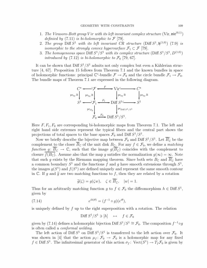
GEOMETRY WITH CONSTRAINTS 109
1. The Virasoro-Bott group V ir with its left invariant complex structure (Vir, vir(0,1))definied by (7.11) is bi-holomorphic to F [79].
2. The group Diff S1 with its left invariant CR structure (Diff S1, h(1,0)) (7.9) isisomorphic to the strongly convex hypersurface F1 ⊂ F [79].
3. The homogeneous space Diff S1/S1 with its complex structure (Diff S1/S1, D(1,0))introduced by (7.12) is bi-holomorphic to F0 [79, 67].
It can be shown that Diff S1/S1 admits not only complex but even a Kahlerian struc-ture [4, 67]. Proposition 15 follows from Theorem 7.1 and the known bundles in spaceof holomorphic functions: principal C∗-bundle F → F0 and the circle bundle F1 → F0.The bundle maps of Theorem 7.1 are expressed in the following diagram.
C5
prby R''
Fprby R
''
!"&& F !! Vir
prby R''
#$
!!&& C5
prby R''
S1 F1
prF0
''
!"&& F1 !! Diff S1&&
prDiff S1/S1
''
#$
!! S1
F0F0 !! Diff S1/S1.&&
Here F, F1, F0 are corresponding bi-holomorphic maps from Theorem 7.1. The left andright hand side extremes represent the typical fibers and the central part shows theprojections of total spaces to the base spaces F0 and Diff S1/S1.
Now we briefly describe the bijective map between F0 and Diff S1/S1. Let Bc
C be thecomplement to the closer BC of the unit disk BC. For any f ∈ F0, we define a matchingfunction g : B
c
C → C, such that the image g(Bc
C) coincides with the complement to
closure f(BC). Assume also that the map g satisfies the normalization g(∞) =∞. Notethat such g exists by the Riemann mapping theorem. Since both sets BC and B
c
C havea common boundary S1 and the functions f and g have smooth extensions through S1,the images g(S1) and f(S1) are defined uniquely and represent the same smooth contourin C. If g and g are two matching functions to f , then they are related by a rotation
g(ζ) = g(ζw), ζ ∈ Bc
C, |w| = 1.
Thus for an arbitrarily matching function g to f ∈ F0 the diffeomorphism h ∈ Diff S1,given by
(7.14) eih(θ) = (f−1 g)(eiθ),
is uniquely defined by f up to the right superposition with a rotation. The relation
Diff S1/S1 $ [h] ↔ f ∈ F0
given by (7.14) defines a holomorphic bijection Diff S1/S1 ∼= F0. The composition f−1gis often called a conformal welding.
The left action of Diff S1 on Diff S1/S1 is transferred to the left action over F0. Itwas shown in [4] that the action µf : F0 → F0 is a holomorphic map for any fixedf ∈ Diff S1. The infinitesimal generator of this action σf : Vect(S1) → TfF0 is given by
110 IRINA MARKINA
the variational formula of A. C. Schaeffer and D. C. Spencer [106, page 32]
σf [u∂θ](z) :=f 2(z)
2π
∫S1
(wf ′(w)
f(w)
)2u(w) dw
w(f(w)− f(z))∈ TfF0.
defined for f ∈ F0, u∂θ ∈ Vect S1. It extends by linearity to a map
L[f, ·] : Vect S1 ⊗ C → TfF0 ⊗ C = T(1,0)f F0 ⊕ T
(0,1)f F0.
The variation L[f, ·] defines also an isomorphism of vector spaces h(1,0) ↔ T(1,0)f F0, which
is given explicitly by(7.15)
Lk[f ] = L[f, ek](z) = zk+1f ′(z), ek = −ieikθ∂θ ∈ h(1,0), Lk[f ] ∈ T(1,0)f F0, k = 1, 2, . . .
by making use of the residue calculus, see e.g.; [4, 66]. Taking the antiholomorphic part
of the basis e−k = ie−ik(θ)∂θ, k = 1, 2, . . . , we obtain expressions for L−k[f ] ∈ T(1,0)f F0
which are rather difficult. The first two of them are
L−1[f ](z) = f ′(z)− 2c1f(z)− 1, L−2[f ](z) =f ′(z)
z− 1
f(z)− 3c1 + (c2
1 − 4c2)f(z),
and others can be obtained by the Witt commutation relations [4, 67]
(7.16) [Lk, Ln] = (n− k)Lk+n, k, n ∈ Z.
The constant vector u0 = −i is mapped to L0[f ](z) = zf ′(z) − f(z). The left invariantvector fields Lk, k ∈ Z were obtained in [67] and received the name of Kirillov’s vectorfields, see also [4]. We have
T(1,0)id F0 = spanL0[id], L1[id], L2[id], . . . = spanz2, z3, . . ..
7.1.5. KdV and Virasoro-Bott group. Let us impose L2-inner product (·, ·)L2 on thealgebra vir by
(7.17)((u(θ)∂θ, a), (v(θ)∂θ, b)
)L2 =
1
2π
∫S1
u(θ)v(θ) dθ + ab.
Then by right translations we define a right invariant L2-metric on the Virasoro-Bottgroup. We are interested in finding a geodesic equation on the group Vir with respectto L2-metric. First we present the Hamiltonian equation on Lie groups. In this case itcan be rewritten as an equation on its dual Lie algebra g∗. We start from the Poissonstructure on the group naturally defined by Lie algebra structure, and then present theHamiltonian equation on g∗ corresponding to this Poisson structure.
Definition 34. The natural Lie-Poisson (or Kirillov-Kostant-Poisson) structure ·, ·defined on the dual Lie algebra g∗ is
·, · : C∞(g∗)× C∞(g∗) → C∞(g∗)(f(w), g(w)) %→ 〈[dwf, dwg], w〉.
GEOMETRY WITH CONSTRAINTS 111
Here, as usual, 〈 , 〉 is the pairing between g and g∗. The functions f, g are fromC∞(g∗), w ∈ g∗ and dwf, dwg ∈ T ∗w(g∗). We identify elements of T ∗w(g∗) with g and thinkof df, dg as elements of Lie algebra g.
Now if f ∈ C∞(g∗), then the Hamiltonian equation takes the form
df(w)
dt= H, f(w) = 〈[dwH, dwf ], w〉 = 〈addwH(dwf), w〉= 〈dwf, ad∗dwH(w)〉
Since the left hand side can be written as 〈dwf, w〉, we get that the Hamiltonian equationon g∗ takes the form
(7.18) w(t) = ad∗dw(t)H(w(t)).
Let A : g → g∗ be any invertible self adjoint operator, e. g. 〈Aξ, w〉 = 〈ξ, Aw〉, where〈 , 〉 is the pairing between g and g∗. Such operators are often called “inertia operator”.Define the Hamiltonian function H : g∗ → R by
H(w) :=1
2〈w, A−1w〉, w ∈ g∗.
Then dwH(w) = A−1w, and the Hamiltonian equation takes the form
(7.19) w(t) = ad∗A−1w(t)(w(t)).
Let us apply this calculus to the Virasoro-Bott group. As we know, the Lie algebravir consists of vector fields (v(θ)∂θ, a). The dual space vir∗ for infinite dimensional spacevir is too large, therefore one usually consideres its “smooth part” in the following sense:for every non-zero element v∂θ ∈ vir there is an element w ∈ vir∗ such that 〈v∂θ, w〉 .= 0and the converse is also true. The dual space vir∗ can be identified with so called smoothquadratic differentials (u(θ)(dθ)2, a), u ∈ C∞(S1, R), see [65]. The pairing is defined by
(7.20)⟨(
u(θ)(dθ)2, a),(v(θ)∂θ, b
)⟩=
1
2π
∫S1
v(θ)u(θ) dθ + ab.
The co-adjoint action of the Lie algebra vir on its dual vir∗ is the following
(7.21) ad∗(v(θ)∂θ ,b
) (u(θ)(dθ)2, a)
=((−2v′u− vu′ − av′′′)(dθ)2, 0
).
Generally, the presence of any inner product ( , ) on a Lie algebra g allows to constructthe inertia operator A by (u, v) = 〈A(u), v〉 for all u, v ∈ g. It is analogous to the situa-tion when a metric on a Riemannian manifold M produces the canonical identificationTqM with its dual T ∗q M , q ∈ M . The L2 product (7.17) and pairing (7.20) define thefollowing the inertia operator
A : vir → vir∗
(u(θ)∂θ, a) %→ (u(θ)(dθ)2, a)
The Hamiltonian function defined by product (7.17) and pairing (7.20) is
H((u(θ)(dθ)2, a)
)=
1
2
∫S1
u2(θ) dθ + a2
112 IRINA MARKINA
and d(u(θ)(dθ)2,a
)H = (u(θ)∂θ, a). Then substituting(u(θ)(dθ)2, a
)for ω in (7.19) we get
d
dt
(u(θ)(dθ)2, a
)=((−3uu′ − au′′′)(dθ)2, 0
).
The last equation is reduced to the system
u = −3uu′ − au′′′,(7.22)
a = 0.
The first equation is the Karteweg-de Vries (KdV) non-linear evolution equation thatdescribes traveling waves in a shallow canal. The second equation is just saying that theparameter a is the real constant.
Remark that the Euler equation for L2 metric on the group Diff S1 is called the Hopfor inviscid Burgers equation. We will obtained it in Subsection 7.2.
Exercises
1. Prove the formula for the co-adjoint action (7.21) using pairing (7.20) and thedefinition 〈ad∗ξ ω, η〉 = −〈ω, adξ η〉 for ξ, η from a Lie algebra and ω from the dualto the Lie algebra.
Other interesting equations. On the groups Diff S1 and Vir more metrics canbe defined. Let us describe them and write the corresponding geodesic equations.
On the Virasosro algebra Vir and on Vect(S1) the following weighted family of metrics(·, ·)H1
α,βcan be defined
(7.23)((v∂θ, a), (u∂θ, b)
)H1
α,β
=
∫S1
(αvu + βv′u′
)dθ + ab.
Theorem 7.2. [63] The Euler equations for the right invariant metric (·, ·)H1α,β
, α .= 0
on the Virasoro-Boot group are given by the following system
α(u + 3uu′)− β(u′′ + 2u′u′′ + uu′′′ + au′′′
)= 0(7.24)
at = 0,
for (u(θ, t)∂θ, a(t)) ∈ Vir for each t ∈ I.
For α = 1, β = 0 equation (7.24) is the KdV equation (7.22). For α = β = 1one recovers Camassa-Holm equation. For α = 0, β = 1 equation (7.24) becomes theHunter-Saxton equation. Note that in the case α = 0 the metric (·, ·)H1
α,βbecomes the
homogeneous dehenerate (·, ·)H1 metric and therefore to define the Euler equation onehas to consider the homogeneous space Diff S1/S1 and define the geodesic flow on it (fordetails see [63]).
Contour dynamics and Virasoro algebra The relations between contour dy-namics, stochastic evolution equations, conformal field theory and groups Vir and Diff S1
were described in [10, 11, 36, 37, 82, 83].
GEOMETRY WITH CONSTRAINTS 113
7.2. Sub-Riemannian geodesics on Diff S1. In this section we present some resultsfor sub-Riemannian geodesics on groups Diff S1 and Vir. First we describe the horizontalsub-bundles and metrics on them. Then we present some formulas for normal geodesicsand discuss the controllability of these groups with respect to chosen horizontal sub-bundles.
7.2.1. Horizontal sub-bundles. Recall that the linear map η : Vect(S1) → R given by
(7.25) η(u∂θ) =1
2π
∫ 2π
0
u(θ) dθ,
associates to each vector field from Vect(S1) its mean value on the circle. The kernel of η,consisting of all vector fields with zero mean value, is isomorphic to Vect(S1)/s1, wheres1 as before denotes the subalgebra of Vect(S1) of constant vector fields, correspondingto the abelian group of rotations S1. We use the notation Vect0(S
1) = Vect(S1)/s1.Then Vect(S1) = Vect0(S
1)⊕ s1.Define a horizontal sub-bundle H of T Diff S1 by left translations of Vect0(S
1). Ahorizontal sub-bundle E of T Vir is left translations of
(Vect0(S
1), 0)
on Vir. Then the
complement of(Vect0(S
1), 0)
in vir is given by
s1 = (a0∂θ, a) ∈ vir : a0, a ∈ Rand we have vir =
(Vect0(S
1), 0)⊕ s1. This is an abelian sub-algebra corresponding to
the abelian sub-group
S1 = (θ %→ θ + b0, b) ∈ Vir : b0, b ∈ R.Proposition 16. The sub-bundle H of T Diff S1 is invariant under the action of rota-
tions S1 and the sub-bundle E of T Vir is invariant under the action of S1.
Proof. If ρ : θ → θ + b0 is a rotation, then
Adρ(u)(θ) =d
dε
∣∣∣ε=0
(b0 + exp(εu(θ − b0)
)= u(θ − b0).
Therefore, η(Adρ(u)) = η(u), which means that H is invariant under the action of S1.
By similar arguments E is invariant under S1. !
7.2.2. Sub-Riemannian metrics and normal geodesics. Let us describe left-invariant met-rics on H and E . We start with H. Let ( , )1,0 denote the standard L2 inner product onVect S1 (
u∂θ, v∂θ)1,0
=1
2π
∫ 2π
0
u(θ)v(θ)dθ.
Let g1,0 be the Riemannian metric obtained by left translation of ( , )1,0, and let h1,0 beits restriction to H.
Before we present the equations for sub-Riemannian normal geodesics with respect tothe metric h1,0, we formulate a more general result that can be found in [52].
Theorem 7.3. Let G be an infinite-dimensional regular Lie group and K be its connectedsubgroup. Denote by g and k their respective Lie algebras. Let ( , ) be an inner productin g for which ad(ξ exists for any ξ ∈ g. Assume that h = k⊥ and g = h⊕ k. Define the
114 IRINA MARKINA
horizontal distribution H by left translations of h. Let g be a Riemannian metric on Gobtained by left translation of ( , ) and h = g|H. The following statements hold.
(a) If ( , ) is ad(k) invariant and if γR : [0, 1] → G is a Riemannian geodesic withrespect to g, then
λ(t) = prk κ7(γR(t)), t ∈ [0, 1]
is constant. Here prk : g → k is the orthogonal projection with respect to ( , ) andκ7(γ(t)) = dγ−1(t)l(γ(t)) is the left logarithmic derivative.
(b) If ( , ) is Ad(K) invariant and if γsR : [0, 1] → G is a sub-Riemannian geodesicwith respect to h, then γsR is a normal geodesic, if and only if, it is of the form
(7.26) γsR(t) = γR(t) · expG(−λt), λ = prk κ7(γR), t ∈ [0, 1],
where γR : [0, 1] → G is a Riemannian geodesic with respect to g.(c) The left logarithmic derivative usR(t) = κ7(γsR(t)) of the curve γsR(t) satisfies
the equation usR(t) = ad(usR(t)(usR(t) + λ) with a constant λ.
To write the equation of an H-horizontal normal geodesic on Diff S1 we have to checkthe conditions of Theorem 7.3 for G = Diff S1 and K = S1. We start from the calculationof the adjoint operator ad(u∂θ
with respect to the inner product ( , )1,0 on Vect(S1), that
is defined by (ad(u∂θv∂θ, w∂θ)
1,0 = (v∂θ, adu∂θw∂θ)
1,0 = (v∂θ, [u∂θ, w∂θ])1,0. We drop the
symbol ∂θ to simplify the notation. We calculate
(ad(u v, w)1,0 = (v,−uw′ + u′w)1,0 =1
2π
∫ 2π
0
(− uvw′ + u′vw)dθ
=1
2π
∫ 2π
0
(uv′ + 2u′v
)w dθ = (uv′ + 2u′v, w)1,0
using integration by parts. Remember that all the functions u, v, w are periodic on[0, 2π], and therefore the term outside of the integral vanishes. We conclude
(7.27) ad(u v = uv′ + 2u′v, u∂θ, v∂θ ∈ Vect(S1)
Proposition 17. The inner product ( , )1,0 is Ad(S1)- and ad(s1)- invariant.
Proof. In general, Ad(S1)- invariance implies ad(s1)- invariance. Nevertheless, we presentboth proofs. It was shown in the proof of Proposition 16 that for the rotation ρ(θ) = θ+bthe adjoint action of ρ ∈ S1 is expressed as Adρ u(θ) = u(θ−b). Then (Adρ u, Adρ v)1,0 =(u, v)1,0, since u, v are periodic with period 2π.
Denote by p0 = ∂θ the basis vector for s1. Then
(adp0 u, v)1,0 = ([p0, u], v)1,0 = −(u′, v)1,0 = (u, v′)1,0 = −(u, [p0, v])1,0 = −(u, ad(p0, v])1,0.
It implies that the inner product ( , )1,0 is invariant under the adjoint action of thealgebra s1. !
Moreover, the subspaces Vect0(S1) and s1 are orthogonal with respect to this inner
product ( , )1,0, making the linear map η from (7.25) an orthogonal projection onto s1.We see that all the hypotheses of Theorem 7.3 are satisfied. Thus, the normal H-
horizontal geodesic γ : I → Diff S1 is the solution to the equations
κ7(γ) = u, u = ad(u (u + λ) = 3uu′ + 2λu′, u ∈ Vect0(S1), λ ∈ R.
GEOMETRY WITH CONSTRAINTS 115
The Riemannian geodesics obtained for λ = 0 are solutions to Burgers’ equation u =3uu′. For the map π : Diff S1 → Diff S1/S1 we denote the base space Diff S1/S1 by B.Let b1,0 be the Riemannian metric on B = Diff S1/S1 obtained as a pushforward of h1,0
by π. Then the Riemannian geodesics in B with respect to b1,0 are projections π(γ).Now we consider a more general family of metrics than just the L2-metric. Define a
two-parameter family ( , )αβ0 of inner products on Vect0(S1) by the formula
(u, v)αβ0 =1
2π
∫ 2π
0
(αu(θ)v(θ) + βu′(θ)v′(θ))dθ, u, v ∈ Vect0(S1).
The inner product is non-degenerate for α .= −n2β, n ∈ N, and is positively definiteonly if β ≥ 0 and α > −β. We extend the inner product ( , )αβ0 to the entire Lie algebraVect(S1) by the formula
(7.28) (u, v)αβ =(u− η(u), v − η(v)
)αβ0
+ η(u)η(v) u, v ∈ Vect(S1).
Let us define a Riemannian metric gαβ by left translation of ( , )αβ , and let hαβ be itsrestriction to H. Theorem 7.3 can be applied also in this case and we deduce that anH-horizontal normal geodesic γ : I → Diff S1 with respect to the metric hαβ is a solutionto the equations
κ7(γ) = u, βu′′ − αu = β(uu′′′ + 2u′u′′)− 3αuu′ + 2λu′, u ∈ Vect0(S1).
If bαβ is the Riemannian metric on B = Diff S1/S1 induced by hαβ as a pushforward,then the Riemannian geodesics on B are given as projections π(γ) of solutions. Thedetails can be found in [52].
Now we present metrics and normal geodesics for the Virasoro-Bott group Virµν , wherethe sub-index corresponds to the 2-cocycle ωµν . We extend the inner product ( , )αβ tothe Virasoro algebra virµν . The extension is given by the formula(
(u∂θ, a1), (v∂θ, a2))αβ
µν= (u, v)αβ + a1a2.
Let gαβµν be the Riemannian metric on Virµν obtained by left translations of ( , )αβµν , and
let hαβµν be its restriction to the sub-bundle E .
Let us calculate the adjoint ad((u,a) of ad(u,a) with respect to the metric ( , )1,0µν . Notice
that
ωµν(u, v) =1
2π
∫ 2π
0
(µu(θ)v′(θ) + νu′(θ)v′′(θ)
)dθ = −(u, Lµνv
′)1,0,
where we used the notation Lµνv = −µv + νv′′. Then we calculate⟨ad((u,a)(v, b), (w, c)
⟩1,0
µν= 〈v, [u, w]〉1,0 − bωµν(w, u)
= 〈ad(u v, w〉1,0 + 〈w, bLµνu′〉1,0(7.29)
=⟨(uv′ + 2u′v + bLµνu
′, 0), (w, c)⟩1,0
µν
by formula (7.27).The conditions of Theorem 7.3 are satisfied. The left logarithmic derivative (u(t), 0) ∈
(Vect0(S1), 0) ⊂ gµν of an E-horizontal normal geodesic (γ, b) : I → Virµν with respect
116 IRINA MARKINA
to the metric h1,0µν is a solution to the equation (u, 0) = ad((u,0)(u + λ1,λ2), λ1,λ2 ∈ R.
This means that the curve (γ, b) is a solution to
(7.30) κ7(γ) = u, with u = 3uu′ + (2λ1 − λ2µ)u′ + λ2νu′′′, u ∈ Vect0(S1).
The corresponding Riemannian geodesics with respect to g1,00,1 satisfy the KdV equation,
as was shown in Subsection 7.1.5 for an analogous right invariant metric. The equationsfor a normal geodesic with respect to the general metric hαβ
µν can be found in [52].
7.2.3. Metrics on H corresponding to invariant Kahlerian metrics. In this subsectionwe discuss metrics on the sub-bundle H of T Diff S1 obtained by the pullback of someKahlerian metrics defined on B = Diff S1/S1. Recall that the left action of Diff S1 onB is well-defined. Let us choose an Hermitian metric on the base space B assumingthat this metric is Kahlerian and invariant under the action of Diff S1. All pseudo-Hermitian metrics on B are included into the two-parameter family bαβ, see [68, 66, 69].We describe the metric identifying B and F0 as it was made in Subsection 7.1.4. It issufficient to describe this metric only at idBC ∈ F0 because at other points of F0 themetric bαβ are defined by the left action of Diff S1. Any smooth curve ft in F0 withf0 = idBC can be written as
ft(z) = z + tzF (z) + o(t), F ∈ A0 .
Hence, we can identify TidBCF0 with A0 by relating the equivalence class [t %→ ft] to F .
With this identification, the metric bαβ ∈ F0 can be written as
bαβ
∣∣idBC
(F1, F2) =2
π
∫∫BC
(αF ′
1F′2 + β(zF ′
1)′(zF ′
2)′)dσ(z),
= 2
∞∑n=1
(αn + βn3)anbn,(7.31)
where dσ(z) is the area element and F1(z) =∑∞
n=1 anzn, F2(z) =
∑∞n=1 bnzn. If α .=
−n2β, n ∈ Z, then the metric bαβ is non-degenerate pseudo-Hermitian. Otherwise, bαβ
degenerates along a distribution of complex dimension 1. Moreover, we require β ≥ 0 and−α < β in order to obtain a positively definite Hermitian metric. Since it is impossibleto write the left action of Diff S1 on F0 explicitly, it is not easy to describe bαβ globallyon F0. However, these metrics can be pulled back to H by projections π : Diff S1 → F0.Consider the injective map
didπ : Vect0 S1 → TidBCF0∼= A0
u∂θ %→ F.
Then the elements F and u are related by the formula, see [68]
F (eiθ) =i
2
(u(θ)− iJu(θ)
).
GEOMETRY WITH CONSTRAINTS 117
where J is from (7.13). Observe that
bαβ|idBC(F1, F2) =
2
π
∫∫BC
(αF ′
1F′2 + β(zF ′
1)′(zF ′
2)′)dσ(z)
=−i
π
∫∫BC
(αdF1 ∧ dF 2 + βd(zF ′
1) ∧ d(zF ′2))
=−i
π
∫S1
(αF1dF 2 + β(zF ′
1)d(zF ′2))
.
So we conclude that for any u, v ∈ Vect0(S1), and F1 = i
2
(u− iJu
), F2 = i
2
(v − iJv
)bαβ |idBC
(didπu, didπv
)=
i
4π
∫S1
(α(u− iJu) d(v + iJv) + β(u′ − iJu′) d(v′ + iJv′)
)=
i
4π
∫S1
(α(u dv − iJu dv + iu dJv + Ju dJv)
+ β(u′ dv′ − iJu′ dv′ + iu′ dJv′ + Ju′ dJv′))
=i
4π
∫S1
(α(u dv + Ju dJv) + β(u′ dv′ + Ju′ dJv′)
)+
1
4π
∫S1
(α(Ju dv − u dJv) + β(Ju′ dv′ − u′ dJv′)
)= iωαβ(u, v) + ωαβ(Ju, v),
where ωαβ is 2-cocycle (7.10) and in the last equation we used∫
S1 u dv =∫
S1 Ju dJvthat can be shown by Fourier expansions. The corresponding to the cocycle ωαβ innerproduct on Vect0(S
1) is obtained by
! u, v "αβ = ωαβ(Ju, v).
Observe that
(7.32) ! u, v "αβ = −(Ju′, v)αβ, u, v ∈ Vect0(S1).
Extend ! , "αβ to an inner product on the whole algebra Vect S1 as in (7.28). Let gαβ
be the Riemannian metric obtained by left translation of ! , "αβ, and let hαβ be themetric restricted to H. We apply Theorem 7.3 and deduce that a normal critical curveγ : I → Diff S1 is the solution to
κ7(γ) = u, −αJu′ + βu′′′ = −α(uJu′′ + 2u′2) + β(uJu′′′′ + 2u′′′) + 2λu′, λ ∈ R.
Here we used the property (7.32), see also [52]. We conclude that the geodesics for bαβ
can be found by solving the above equation for λ = 0 and then projecting them to F0.For (α, β) = (1, 0), this is a special case of the modified Constantin-Lax-Majda (CLM)
equation. For more information, see [35], where the Riemannian geometry of g1,0 isconsidered.
118 IRINA MARKINA
7.2.4. Controllability on Diff S1. Before we formulate the main result in controllability,we describe some special subgroups of Diff S1.
We start from subalgebras of Vect S1. For each n ∈ Z, let us define
pn = cos nθ ∂θ, kn = sin nθ ∂θ.
The Lie brackets are given by
(7.33) [km, kn] = m+n2
km−n + m−n2
km+n,
(7.34) [pm, pn] = −m+n2
km−n − m−n2
km+n,
(7.35) [pm, kn] = −m+n2
pm−n + m−n2
pn+m.
It is easy to see from (7.33–7.35) that hn = spanp0, pn, kn are subalgebras ofVect(S1), and that hn is isomorphic to su(1, 1) for each n. To each Lie sub-algebrahn ⊂ Vect(S1) corresponds a subgroup Hn of Diff S1.
To show that any two points on groups Diff S1 or Vir can be connected by H- or,respectively, E-horizontal curve, we use the invariance of these horizontal sub-bundlesunder the corresponding group action. We start from a general result. Assume that ahorizontal sub-bundle H is invariant under the action of some subgroup K of a givengroup G. Then, if the tangent bundle TK is transversal to H, the question of controlla-bility is reduced to the question whether elements of K can be reached from the unityof G by an H-horizontal curve.
Lemma 7. Let G be a Lie group with the Lie algebra g, and let a left- (or right-)invariant horizontal sub-bundle H be obtained by left (or right) translations of a subspaceh ⊆ g. Assume that there is a sub-group K of G with the Lie algebra k such that g = p⊕ kfor some p ⊆ h. Suppose also that h is Ad(K)-invariant. Then any pair of elements inG can be connected by a smooth H-horizontal curve, if and only if, for every a ∈ K thereis an H-horizontal smooth curve connecting 1 ∈ K and a.
Proof. We present the proof for the case of a left-invariant sub-bundle H. Let c : [0, 1]→G be any curve (not necessarily horizontal), connecting the points a0 and a1, and havingleft logarithmic derivative u. Using left translation of c by a−1
0 , we can assume thata0 = 1. Let prk : g → k be the projection with the kernel p ⊂ h.
Consider the projection k(t) = prk u(t), t ∈ [0, 1]. Let ϑ be a curve in K with leftlogarithmic derivative k, starting at 1. Then the left logarithmic derivative of the curveϑ(t)−1 is −Adϑ k.
Let us show that the curve γ1(t) = c(t) · ϑ(t)−1 is H-horizontal. We calculate the leftlogarithmic derivative of γ1(t) and find
κ7(∂t(c(t) · ϑ(t)−1)) = Adϑ(t)(u(t)− k(t)) ∈ h,
since h is Ad(K) invariant. Hence, we have constructed an H-horizontal curve γ1, from 1to a1 ·ϑ(1)−1. Applying the right translation by ϑ(1), that keeps the curve H-horizontalbecause of the Ad(K)-invariance of h, we get a curve from ϑ(1) to a1. Moreover, by thehypothesis of the theorem, we can connect 1 with ϑ(1) by a smooth horizontal curve γ2.Finally, we glue the curves γ1 and γ2 into one smooth curve by slowing exponentiallydown to zero speed at the connecting point. !
GEOMETRY WITH CONSTRAINTS 119
Theorem 7.4. The following is true.
(a) Let H be a choice of a horizontal sub-bundle on Diff S1 defined as in Section 7.2.1.Then any pair of points can be connected by an H-horizontal curve.
(b) Let E be a choice of a horizontal sub-bundle on Virµν defined as in Section 7.2.1.Then any two points on Virµν can be connected by an E-horizontal curve.
Proof. To prove (a), it is sufficient to show that any two points in Diff S1 can beconnected by an H-horizontal curve. Due to Lemma 7, we only need to verify thatid ∈ Diff S1 can be connected with any element in S1 by an H-horizontal curve. Thesubgroup S1 is contained in Hn for any n, in particular, S1 can be considered as asubgroup of H1. Any H-horizontal curve in H1, will have left logarithmic derivativein h1 ∩Vect0(S
1) = spank1, p1. Since [p1, k1] = p0, the horizontal distribution H re-stricted to H1 is bracket generating. The group H1 is finite-dimensional, therefore wecan apply the Rashevskiı-Chow theorem to conclude that every point in H1, includingpoints in S1, can be reached by an H-horizontal curve.
To prove (b), we need to show that any point in S1 = θ %→ (θ + a, b) ∈ Virµν canbe connected to (id, 0) ∈ Virµν by an E-horizontal curve. Let
Hn = (φ, a) ∈ Virµν : φ ∈ Hn, a ∈ R .
which has Lie algebra
hn = span (p0, 0), (pn, 0), (kn, 0), (0, 1) .
Unfortunately, the sub-bundle restricted to the group Hn is not bracket generating. We
need to find a smaller subgroup. The Lie algebras hn have special subalgebras
tn = span(p0, n
2ν − µ), (pn, 0), (kn, 0)
.
Denote the corresponding subgroups by Tn. On the contrary to what holds on Hn, the
distribution E restricted to any subgroup Tn is bracket generating, and so all elements
in such a subgroup Tn can be reached by an E-horizontal curve. It is clear that
Tn ∩ S1 =(
θ %→ θ + r, r(n2ν − µ))
: r ∈ R
,
where S1 is the subgroup of translations in H1. Since S1 is isomorphic to R2 as a group
and ν .= 0, we can find unique elements gj ∈ Tj∩S1, j = 1, 2 such that g = g1 ·g2 = g2 ·g1
for any g ∈ S1. Denote by c1 and c2 curves that connect (id, 0) ∈ Virµν with g1 and g2,respectively. We can reach g by first following a curve c2 and then moving to g by acurve from g2 c1 to g1, that is the translation of c1 by g2. This finishes the proof. !
8. Appendix A
8.1. Smooth manifolds.
Definition 35. A topological space S is second countable if its topology has a countablebase, that is a countable collection B of open sets such that every open set is the unionof some sub-collection B.
Definition 36. A set P is a submanifold of a manifold M if:
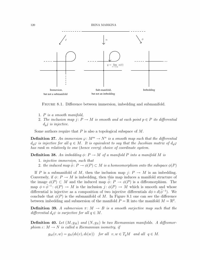
120 IRINA MARKINA
ϕ
q = limt→+∞
α(t)
Immersion,but not a submanifold
Sub-manifold,but not an imbedding
φ
Imbedding
α
Figure 8.1. Difference between immersion, imbedding and submanifold.
1. P is a smooth manifold,2. The inclusion map j : P → M is smooth and at each point p ∈ P its differential
dpj is injective.
Some authors require that P is also a topological subspace of M .
Definition 37. An immersion ϕ : Mm → Nn is a smooth map such that the differentialdqϕ is injective for all q ∈ M . It is equivalent to say that the Jacobian matrix of dqϕhas rank m relatively to one (hence every) choice of coordinate system.
Definition 38. An imbedding φ : P →M of a manifold P into a manifold M is
1. injective immersion, such that2. the induced map φ : P → φ(P ) ⊂ M is a homeomorphism onto the subspace φ(P )
If P is a submanifold of M , then the inclusion map j : P → M is an imbedding.Conversely, if φ : P → M is imbedding, then this map induces a manifold structure ofthe image φ(P ) ⊂ M and the induced map φ : P → φ(P ) is a diffeomorphism. The
map φ φ−1 : φ(P ) → M is the inclusion j : φ(P ) → M which is smooth and whose
differential is injective as a composition of two injective differentials dφ d(φ−1). Weconclude that φ(P ) is the submanifold of M . In Figure 8.1 one can see the differencebetween imbedding and submersion of the manifold P = R into the manifold M = R2.
Definition 39. A submersion π : M → B is a smooth surjective map such that thedifferential dqψ is surjective for all q ∈ M .
Definition 40. Let (M, gM) and (N, gN) be two Riemannian manifolds. A diffeomor-phism ι : M → N is called a Riemannian isometry, if
gM(v, w) = gN(dι(v), dι(w)) for all v, w ∈ TqM and all q ∈ M.
GEOMETRY WITH CONSTRAINTS 121
Definition 41. Let (M, gM) and (B, gB) be two Riemannian manifolds and let π : M →B be a submersion. Then let TqM = ker(dqπ)⊕⊥
(ker(dqπ)
)⊥be the orthogonal decom-
position with respect to the metric gM . If the restriction dπ|ker(dqπ) : ker(dqπ) → Tπ(q)Bis a linear isometry for any q ∈ M , then the map π is called the Riemannian submersion.
Definition 42. A pairing between the tangent and the co-tangent bundle is a map
〈·, ·〉 : TqM × T ∗q M → Rwhich is bi-linear, non-degenerate, and smoothly varying with respect to q ∈ M . It isnon-degenerate in the sense that if 〈v,λ〉 = 0 for all v ∈ TqM then λ = 0.
Definition 43. A curve c : I → M is an integral curve of a vector field X ∈ Vect(M)if it satisfies the differential equation
c(t) = X(c(t)), for all t ∈ I.
A vector field X is complete if each of its non-extendable integral curves (starting fromdifferent points q ∈ M) is defined on I = R. Let us denote by cq,X the integral curveof a complete vector field X starting at q ∈ M . The curve cq,X is just a solution of theCauchy problem
c(t) = X(c(t)), c(0) = q, t ∈ R.
Definition 44. The flow of a complete vector field X on a smooth manifold M is the
map X : R×M →M given by
X(t, q) = cq,X(t),
where cq,X is the non-extendable integral curve of X starting at q ∈ M .
Proposition 18. The flow X of a complete vector field satisfies the conditions:
1. X(0, ·) : M → M is the identity map of M ,
2. X(s + t, ·) = X(s, (X(t, ·)) = X(s, ·) X(t, ·) for all s, t ∈ R. As a corollary we
conclude that flows commute for fixed times,
3. the map X(s, ·) : M → M is a diffeomorphism for any s ∈ R, where the inverse
map is X−1(s, ·) := X(−s, ·).We need the completeness assumption in order to work with the entire manifold M
and not only locally. For arbitrary vector fields one can define a local analogue of theflow.
Now we define a Levi-Civita connection. We start from the definition of the affineconnection.
Definition 45. An affine connection ∇ on a smooth manifold M is a map
∇ : Vect M ×Vect M → Vect M(X, Y ) %→ ∇XY,
satisfying the following properties
1. ∇fX+gY Z = f∇XZ + g∇Y Z,2. ∇X(Y + Z) = ∇XY +∇XZ, for all X, Y, Z ∈ Vect M and f, g ∈ C∞(M).
122 IRINA MARKINA
3. ∇X(fY ) = f∇XY + X(f)Y ,
The notion of the affine connection leads to the definition of the covariant derivativealong a given curve. Namely, let an affine connection ∇ be defined on a smooth manifoldM . Suppose that c : I →M is a smooth curve and X is the vector field along the curve c.Then there exists a unique correspondence which associates to a vector field X anothervector fields DX
dtalong c by the rule
DX
dt:= ∇cX(c(t)).
The covariant derivative Ddt
satisfies the properties
D
dt(X + Y ) =
DX
dt+
DY
dt,
D
dt(fX) =
df
dtX + f
D
dtX.
Definition 46. An affine connection ∇ on a smooth manifold M is symmetric if
∇XY −∇Y X = [X, Y ] for all X, Y ∈ Vect M.
Definition 47. Let (M, g) be a Riemannian manifold with an affine connection ∇. Wesay, that the affine connection ∇ is compatible with the Riemannian metric g if
Xg(Y, Z) = g(∇XY, Z) + g(Y,∇XZ) for all X, Y, Z ∈ Vect M.
The following theorem asserts that the existence of the Riemannian metric guaranteesthe existence of an affine connection that is compatible with the Riemannian metric andsymmetric.
Theorem 8.1. [21, 99] Given a Riemannian manifold (M, g) there is an affine connec-tion ∇, called the Levi-Civita connection, such that ∇ is symmetric and compatible withthe metric g.
8.2. Symplectic manifolds. Let N be a smooth manifold and Ω be a non-degenerateskew symmetric real valued 2-form. Then the pair (N,Ω) is called the symplectic mani-fold.
Definition 48. Let H ∈ C∞(N) be a function, then the associated with H Hamiltonian
vector field−→H is defined by
Ω(X,−→H ) := dH(X) for all X ∈ TN.
The Poisson brackets between H, K ∈ C∞(N) is the directional derivative of one func-tion in the direction of the Hamiltonian vector field, associated with another function.Namely,
H, K := dK(−→H ) = Ω(
−→H,−→K ).
As an example, consider a smooth manifold M and its co-tangent bundle T ∗M . Recallthat if pr∗M : T ∗M →M is the canonical projection, then d(pr∗M) : T (T ∗M) → TM . Weuse the notation 〈·, ·〉 to denote the pairing between TM and T ∗M . Define real valuedone-form ω : T (T ∗M) → R on the manifold N = T ∗M by
ω(q,λ)(v) := 〈λ, d(pr∗M)(v)〉, v ∈ T(q,λ)(T∗M).
Then the 2-form Ω = dω is a symplectic form. Verify it!
GEOMETRY WITH CONSTRAINTS 123
If we chose a chart(U,ϕ = (x1, . . . , xn)
)on M , then it induces the chart(
T ∗U,Φ = (x1, . . . , xn,λ1, . . . ,λn))
on T ∗M . The canonical projection pr∗M and its differential take the matrix form
pr∗M =
(In×n 0
0 0
)=⇒ d pr∗M =
(In×n 0
0 0
).
Therefore, the one-form at point (q,λ) = (x1, . . . , xn,λ1, . . . ,λn) is written as ω(q,λ) =∑nj=1 λjdxj . The symplectic form Ω becomes Ω =
∑nj=1 dλj ∧ dxj. The Hamilton-
ian vector field is−→H (q,λ) =
∑nj=1
(∂H∂λj
∂∂xj − ∂H
∂xj∂
∂λj
), and the Poisson brackets are
H, K =(
∂H∂λj
∂K∂xj − ∂H
∂xj∂K∂λj
). To each vector field X ∈ Vect(M) we associate the
function HX : T ∗M → R byHX(q,λ) = 〈λq, X(q)〉.
Then one can associate the Hamiltonian vector field−→HX to the function HX in the
following way. If X(q) =∑n
k=1 Xk(x1, . . . , xn)∂k and λq =∑n
j=1 λj(x1, . . . , xn)dxj then
HX(q,λ) =∑n
j=1 λjXj(q) and
−→HX(q,λ) =
n∑j=1
(Xj(q)
∂
∂xj−[ ∂
∂xj
( n∑k=1
λkXk(q)
)] ∂
∂λj
).
Now it is obvious that
d(pr∗M)(−→HX(q,λ)) = X(q) for all (q,λ) ∈ T ∗M.
Corollary 9. Geodesics produced by the Hamiltonian function HX coincide with integralcurves of the vector field X.
If X ∈ Vect(M), then the vector field−→HX is called the Hamiltonian lift of X .
Exercises.
1. Verify that (C∞(N), ·, ·) is a Lie algebra and the map H %→ −→H is a Lie algebra
homomorphism from
(C∞(N), ·, ·) −→ (Vect N, [·, ·]).2. Show that HX , HY = H[X,Y ] for all X, Y ∈ Vect(M). Conclude that the map
X %→ HX produces a homomorphism of Lie algebras
(Vect(M), [·, ·]) −→ (C∞(T ∗M), ·, ·).8.3. Lie groups. The content of this subsection can be found in [34, 70, 91, 113].
Definition 49. A Lie group G is a smooth (finite dimensional) manifold M and a groupsuch that
multiplication ρ : M ×M → M,(τ, q) → τq
andinversion in : M → M,
x → x−1
are smooth maps of smooth manifolds: M ×M →M and M →M , respectively.
124 IRINA MARKINA
It is customary to use the letter G to denote the underlying manifold M and the pair(M, ρ) in the case of Lie groups.
Definition 50. A Lie algebra g over R (C) is a real (complex) vector space V togetherwith an operation [·, ·] : V × V → V (called the bracket, or Lie product) satisfying thefollowing three axioms:
1. skew symmetry: [X, Y ] = −[Y, X ],2. bi-linearity: [aX + bY, Z] = a[X, Z] + b[Y, Z], a, b ∈ R (C) (and the same with
respect to the second term),3. Jacobi identity: [[X, Y ], Z] + [[Z, X ], Y ] + [[Y, Z], X ] = 0
for any X, Y, Z ∈ V .
We will use the letter g to denote the underlying vector space V in the case of Liealgebras.
Example 10.
1. The general linear group GL(n, R) = GL(n) is the Lie group of all (n × n)-matrices L with real entries such that det L .= 0. Since the determinant functiondet : Rn2 → R is smooth, the underlying manifold of GL(n) is an open subset in
Rn2defined by the inverse image of the determinant function of the value 0 ∈ R.
The group multiplication is the multiplication of matrices. The correspondingLie algebra gl(n, R) = gl(n) is formed by all (n× n)-matrices. The commutatorin GL(n) is the commutator of two matrices. The group GL(n) is the groupof all non-degenerate linear transformations of Rn. In a similar way the groupGL(n, C) can be defined.
2. The orthogonal group O(n, R) = O(n) is the subspace of GL(n) such thatLtrL = LLtr = Id, where Ltr is the transpose to L. The special orthogonal groupSO(n, R) = SO(n) is the subset of O(n) whose matrices have determinant 1.Both groups have the same Lie algebra o(n) consisting of (n× n)-matrices thatare skew symmetric: Ltr = −L. The main feature of these groups is that undertheir transformations the Euclidean inner product in Rn is preserved. (Why?)
3. The unitary group U(n) is the group of (n × n)-matrices with complex entriessuch that LtrL = LLtr = Id, where Ltr is the transposed and conjugate matrixto L. The special unitary group SU(n) is the subset of U(n) whose matriceshave determinant 1. The Lie algebra u(n) is the set of (n × n)-matrices thatare skew-Hermitian symmetric: Ltr = −L. The Lie algebra su(n), n ≥ 2, is thesubset of u(n) having vanishing trace. The unitary and special unitary groupspreserve Hermitian product (z, w) =
∑nk=1 zkwk in Cn.
4. The symplectic group Sp(n) is a group of (n × n)-matrices with quaternionentries such that LtrL = LLtr = Id, where Ltr is the transposed and quaternionconjugate matrix to L. The Lie algebra sp(n) is the set of (n × n)-matricesthat are skew-Hermitian symmetric: Ltr = −L. Symplectic groups preserveHermitian product in the n-dimensional quaternionic space Qn.
5. The special Euclidean group SE(n), or the group of rigid motions in Rn is thegroup consisting of rotations and translations in Rn. An element τ ∈ SE(n) is

GEOMETRY WITH CONSTRAINTS 125
usually written as a pair τ = (A, a), where A ∈ SO(n) and a is a n-dimensionalvector. The multiplication is given by τυ = (A, a)(B, b) := (AB, Ab + a). Thusthe group SE(n) is the group of all isometries in the Euclidean space. Its di-
mension is n(n+1)2
, where n stands for translations and n(n−1)2
is the dimension ofSO(n).
We define the exponential map and list its properties. Let (R, +) be the additivegroup of real numbers and r be the corresponding Lie algebra with generator d
dr. Let
G be a Lie group, g be its Lie algebra, and X ∈ g be an arbitrary element. Then themap h
r $ td
drh%→ tX ∈ g
is a homomorphism of the Lie algebra r into the Lie algebra g. The theorems of Liegroup theory [70, 113] ensure that there is a unique Lie group homomorphism cX , suchthat
cX : R → G, and d cX = h, or dcX(td
dr) = tX.
In other words, the curve cX : R → G is a one-parametric subgroup of G and it is suchthat cX(0) = e and cX(0) = X(e). The curve cX(t), t ∈ R is called the exponential curveand it is often denoted by exp(tX), t ∈ R. The map
exp : g → GX %→ exp(X).
is called the exponential map. We list the properties of the exponential map in thefollowing theorem.
Theorem 8.2. [70, 113] Let X belong to the Lie algebra g of a finite dimensional Liegroup G. Then the following properties hold.
1. The exponential curve exp(tX) = cX(t) for each t ∈ R satisfies
d
dt
∣∣∣t=0
exp(tX) =d
dt
∣∣∣t=0
cX(t) = cX(0) = X,
(see also the definition of the exponential curve in Subsection 3.1).2.
(exp(t1 + t2)X
)=(exp(t1X)
)(exp(t2X)
), for all t1, t2 ∈ R.
3. exp(−tX) =(exp(tX)
)−1for each t ∈ R.
4. The map exp : g → G is a C∞-map between two manifolds.5. The differential at zero vector of the exponential map d exp : T0g → TeG is the
identity map g → g, where we identify elements of g with T0g and with TeG. Animportant corollary is that exp gives a diffeomorphism between a neighborhood of0 ∈ g and a neighborhood of e ∈ G.
6. The left translation of cX by τ ∈ G given by c = lτ (cX(t)) = τcX(t) is the unique
integral curve of the left invariant vector field X such that it starts at the pointτ : c(0) = τ . As a particular consequence, left invariant vector fields are alwayscomplete.
7. The one-parametric flow of diffeomorphisms X(t, τ) : G → G associated with a
left invariant vector field X is given by X(t, τ) = τcX(t) = rcX(t)τ .
126 IRINA MARKINA
8. In the neighborhoods of 0 ∈ g and e ∈ G, where exp is a diffeomorphism, theinverse map is defined and is called logarithm. It expresses the product of twoexponents through the Baker-Campbell-Hausdorff formula [105], whose first termsare given as follows
(8.1) exp(X) exp(Y ) = exp(X + Y +
1
2[X, Y ] +
1
12[X, [X, Y ]]− 1
12[Y, [X, Y ]] + . . .
).
As we see the straight line tX ∈ g is mapped to the one-parametric subgroupexp(tX) ∈ G, t ∈ R.
Definition 51. A subgroup N of a group G is called a normal subgroup if it is invariantunder conjugation; that is, for each element n ∈ N and each τ ∈ G the element τnτ−1 ∈N .
Definition 52. A group G is called simple if it is a non-trivial group and there are noother normal subgroups except the trivial group and the group itself.
A group that is not simple can be decomposed into two smaller groups, a normalsubgroup and the corresponding quotient group, and the process can be repeated.
8.3.1. Action of Lie groups on manifolds. Let M be a smooth manifold and let G be aLie group.
Definition 53. An action of G on M on the left is a smooth map µ : G×M →M suchthat
µ(ςτ, q) = µ(ς, µ(τ, q)), µ(e, q) = q
for all ς, τ ∈ G and q ∈ M .
If µ : G×M →M is an action of G on M on the left, then for a fixed ς ∈ G the mapq %→ µ(ς, q) is a diffeomorphism of M which we will denote by µς . Similarly we define aright action.
Definition 54. An action of G on M on the right is a smooth map µ : M × G → Msuch that
µ(q, ςτ) = µ(µ(q, ς), τ), µ(q, e) = q
for all ς, τ ∈ G and q ∈ M .
We also use the notation τ.q instead of µ(τ, q) for the left action and q.τ instead ofµ(q, τ) for the right action.
Definition 55. We say that a Lie group G acts freely on the right on a smooth manifoldM if for all q ∈ M , q.τ = q.ς if and only if τ = ς. Equivalently; if there exists q ∈ Msuch that q.τ = q (that is, if τ has at least one fixed point), then τ is the identity elemente ∈ G.
Definition 56. We say that G acts transitively on the right on M if for any q, p ∈ Mthere is τ ∈ G such that q.τ = p.
The same definitions can be given for the left action of the group G on a manifold M .
Example 11.
GEOMETRY WITH CONSTRAINTS 127
1. The flow on M defined in Definition 44 is an example of the action of the group(R, +) on a smooth manifold M .
2. The action µ : GL(n)×Rn → Rn of the general linear group in Rn is defined bythe multiplication of (n× n)-matrix by an n-vector (or (1× n)-matrix).
3. Let Sn−1 = x ∈ Rn| ‖x‖E = 1. The action µ : O(n)× Sn−1 → Sn−1 is definedby a multiplication of (n× n)-matrix from O(n) by n-vector having length one.
4. The multiplication law in any Lie group G produces two actions: left and righttranslations. Recall that the action
l : G×G → G(τ, υ) %→ τυ,
or l(τ, υ) = lτ (υ) = τ.υ := τυ, is the left translation and
r : G×G → G(υ, τ) %→ υτ,
or r(υ, τ) = rτ (υ) = υ.τ := υτ is the right translation.5. Define a left action a of a Lie group G on itself G by
(8.2)a : G×G → G
(τ, υ) %→ τυτ−1,
or a(τ, υ) = aτ (υ) = τ.υ := τυτ−1. This action is called the action by conjugationor the inner automorphism. This action produces other very interesting actionsof G on its the Lie algebra g and even an action of the Lie algebra g over itself,see Example (14).
6. Define a left action of a group G on its tangent bundle TG by
(8.3)µ : G× TG → TG
τ.(q, vq) %→ (τq, dqlτ (vq)
).
The right action of G on TG is defined analogously.7. Define a left action of a group G on its co-tangent bundle T ∗G by
(8.4)µ : G× T ∗G → T ∗G
τ.(q,ωq) %→ (τq, (dqlτ )
∗(ωq)),
where (dqlτ )∗ the dual map to the differential dqlτ . The right action of G on T ∗G
is defined analogously.8. The Adjoint action of a Lie group G on its Lie algebra g is defined by
(8.5)µ : G× g → g
(τ, ξ) %→ Adτ (ξ)
The definition of the adjoint map Adτ : g → g see in Example 13. The adjointaction uses the definition of the action a by conjugation (8.2) which is a leftaction. Therefore the action Ad is an action on the left.
9. The co-adjoint action of a Lie group G on its dual to Lie algebra g∗ is defined by
(8.6)µ : G× g∗ → g∗
(τ,ω) %→ Ad∗τ (ω)
See the definition of the co-adjoint map Ad∗τ : g∗ → g∗ in (8.9).
128 IRINA MARKINA
10. An action on the left of the special Euclidean group SE(n) over Rn is defined by
µ : SE(n)× Rn → Rn
(A, a).x %→ Ax + a.
To proceed with examples of action of a Lie group G on its Lie algebra g (the un-derlying manifold is just the vector space TeG) we make some observations about thedifferential map at the identity of the action µ on G. Let
µ : G×G → G.
Fix one variable τ ∈ G and consider
µτ : G → G
as a diffeomorphism of the group G. Then the differential at e ∈ G is the linear map
deµτ : TeG → Tµτ (e)G = TτG.
Let us consider three examples of an action µ: translations r, l, and the action byconjugation a.
Example 12. Let µ be the right translation r : G × G → G, rτ (q) = q.τ . We want tolook at how q.τ changes with respect to the variable τ near τ = 1. This variation iscalled the infinitesimal generator of the right action rτ (q) at point q and is denoted byσq. To calculate σq we observe that the map q.τ with fixed q and variable τ is just theleft translation q.τ = lq(τ), so
σq = delq : TeG → Tlq(e)G = TqG,
or it is customary to write
σq : g → TqG.
We conclude that the map σq generates a left invariant vector field on G, since it trans-lates an element ξ of the Lie algebra g to a vector field Xq = delq(ξ) that will be leftinvariant by definition. In a practical way the map σq is calculated by making use of theexponential curve by the following
(8.7) σq(ξ) =d
dε
∣∣∣ε=0
q exp(εξ) =d
dε
∣∣∣ε=0
lq(exp(εξ)) = dlqd(exp(εξ)|ε=0
)= dlq(ξ).
Analogously, the left translation l has it infinitesimal generator, that is the map g→TqG generating right invariant vector fields. The formula corresponding to (8.7) is
(8.8) σq(ξ) =d
dε
∣∣∣ε=0
exp(εξ))q =d
dε
∣∣∣ε=0
rq(exp(εξ)) = drq(ξ).
Example 13. Now we consider µ = a,
a(τ, q) = aτ (q) = τqτ−1 : G → G,
which is not only the diffeomorphic map of the underlying manifold of the group G, butit also preserves the group structure, so the map aτ is a group automorphism and wewrite aτ ∈ Aut(G). The differential of aτ at the identity is
deaτ : TeG → Taτ (e)G = TeG.
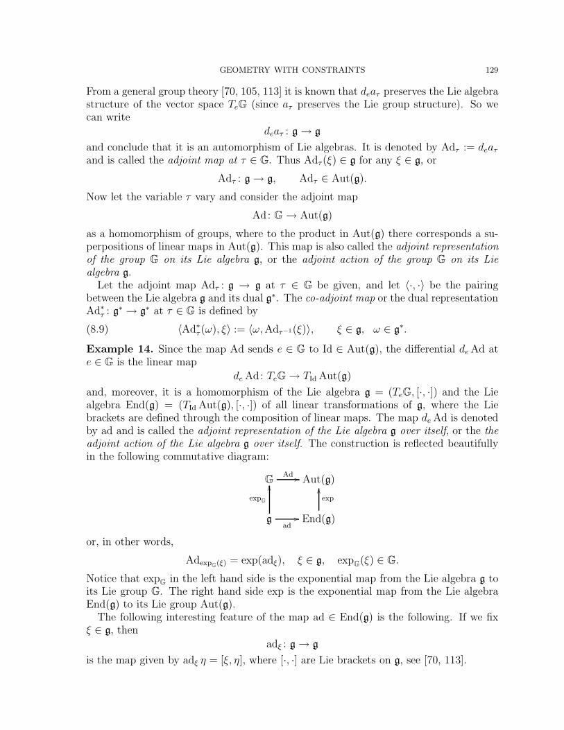
GEOMETRY WITH CONSTRAINTS 129
From a general group theory [70, 105, 113] it is known that deaτ preserves the Lie algebrastructure of the vector space TeG (since aτ preserves the Lie group structure). So wecan write
deaτ : g → g
and conclude that it is an automorphism of Lie algebras. It is denoted by Adτ := deaτ
and is called the adjoint map at τ ∈ G. Thus Adτ (ξ) ∈ g for any ξ ∈ g, or
Adτ : g→ g, Adτ ∈ Aut(g).
Now let the variable τ vary and consider the adjoint map
Ad: G → Aut(g)
as a homomorphism of groups, where to the product in Aut(g) there corresponds a su-perpositions of linear maps in Aut(g). This map is also called the adjoint representationof the group G on its Lie algebra g, or the adjoint action of the group G on its Liealgebra g.
Let the adjoint map Adτ : g → g at τ ∈ G be given, and let 〈·, ·〉 be the pairingbetween the Lie algebra g and its dual g∗. The co-adjoint map or the dual representationAd∗τ : g∗ → g∗ at τ ∈ G is defined by
(8.9) 〈Ad∗τ (ω), ξ〉 := 〈ω, Adτ−1(ξ)〉, ξ ∈ g, ω ∈ g∗.
Example 14. Since the map Ad sends e ∈ G to Id ∈ Aut(g), the differential de Ad ate ∈ G is the linear map
de Ad: TeG → TId Aut(g)
and, moreover, it is a homomorphism of the Lie algebra g = (TeG, [·, ·]) and the Liealgebra End(g) = (TId Aut(g), [·, ·]) of all linear transformations of g, where the Liebrackets are defined through the composition of linear maps. The map de Ad is denotedby ad and is called the adjoint representation of the Lie algebra g over itself, or the theadjoint action of the Lie algebra g over itself. The construction is reflected beautifullyin the following commutative diagram:
G Ad !! Aut(g)
g
expG
((
ad!! End(g)
exp
((
or, in other words,
AdexpG(ξ) = exp(adξ), ξ ∈ g, expG(ξ) ∈ G.
Notice that expG in the left hand side is the exponential map from the Lie algebra g toits Lie group G. The right hand side exp is the exponential map from the Lie algebraEnd(g) to its Lie group Aut(g).
The following interesting feature of the map ad ∈ End(g) is the following. If we fixξ ∈ g, then
adξ : g → g
is the map given by adξ η = [ξ, η], where [·, ·] are Lie brackets on g, see [70, 113].
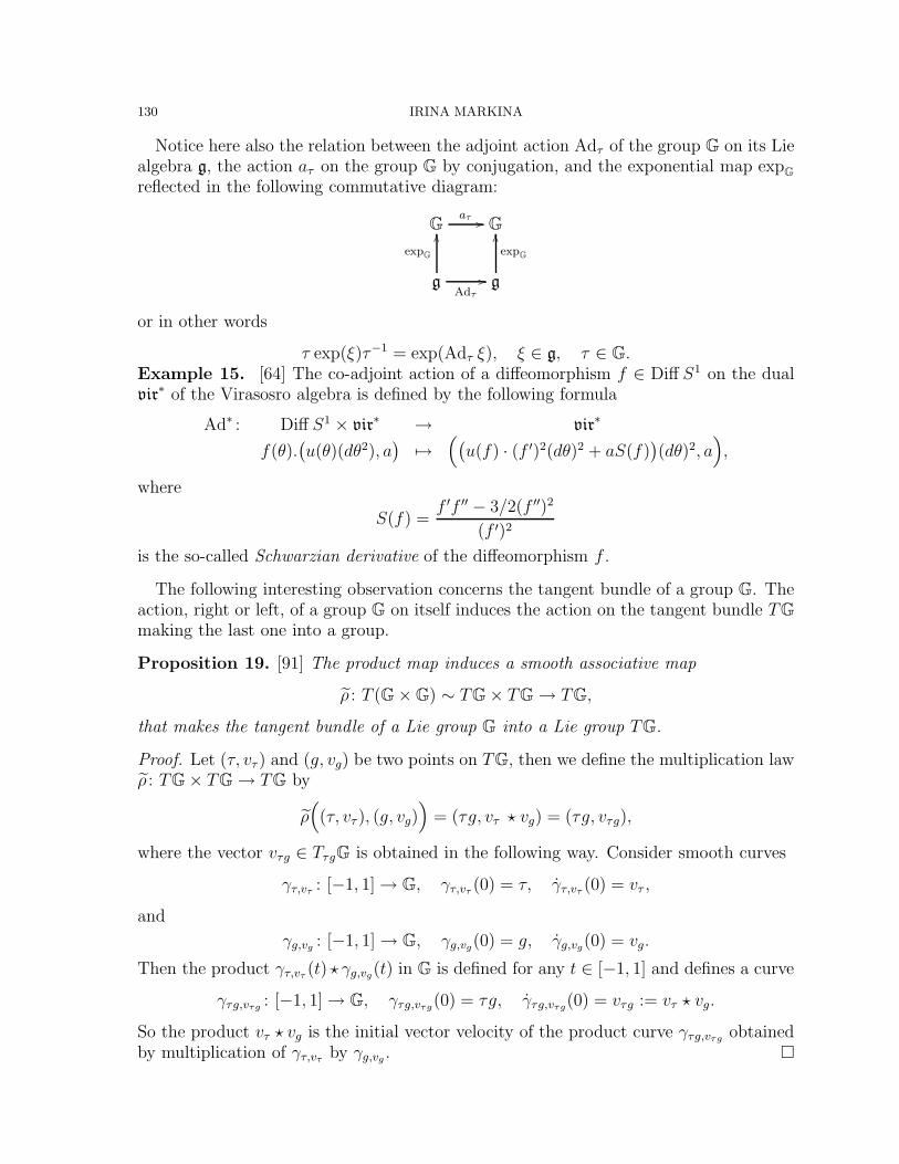
130 IRINA MARKINA
Notice here also the relation between the adjoint action Adτ of the group G on its Liealgebra g, the action aτ on the group G by conjugation, and the exponential map expGreflected in the following commutative diagram:
G aτ !! G
g
expG
((
Adτ
!! g
expG
((
or in other words
τ exp(ξ)τ−1 = exp(Adτ ξ), ξ ∈ g, τ ∈ G.Example 15. [64] The co-adjoint action of a diffeomorphism f ∈ Diff S1 on the dualvir∗ of the Virasosro algebra is defined by the following formula
Ad∗ : Diff S1 × vir∗ → vir∗
f(θ).(u(θ)(dθ2), a
) %→((
u(f) · (f ′)2(dθ)2 + aS(f))(dθ)2, a
),
where
S(f) =f ′f ′′ − 3/2(f ′′)2
(f ′)2
is the so-called Schwarzian derivative of the diffeomorphism f .
The following interesting observation concerns the tangent bundle of a group G. Theaction, right or left, of a group G on itself induces the action on the tangent bundle TGmaking the last one into a group.
Proposition 19. [91] The product map induces a smooth associative map
ρ : T (G×G) ∼ TG× TG → TG,
that makes the tangent bundle of a Lie group G into a Lie group TG.
Proof. Let (τ, vτ ) and (g, vg) be two points on TG, then we define the multiplication lawρ : TG× TG → TG by
ρ((τ, vτ ), (g, vg)
)= (τg, vτ ? vg) = (τg, vτg),
where the vector vτg ∈ TτgG is obtained in the following way. Consider smooth curves
γτ,vτ : [−1, 1]→ G, γτ,vτ (0) = τ, γτ,vτ (0) = vτ ,
and
γg,vg : [−1, 1] → G, γg,vg(0) = g, γg,vg(0) = vg.
Then the product γτ,vτ (t) ? γg,vg(t) in G is defined for any t ∈ [−1, 1] and defines a curve
γτg,vτg : [−1, 1]→ G, γτg,vτg(0) = τg, γτg,vτg(0) = vτg := vτ ? vg.
So the product vτ ? vg is the initial vector velocity of the product curve γτg,vτg obtainedby multiplication of γτ,vτ by γg,vg . !
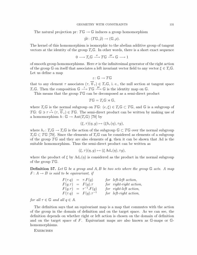
GEOMETRY WITH CONSTRAINTS 131
The natural projection pr : TG → G induces a group homomorphism
pr : (TG, ρ) → (G, ρ).
The kernel of this homomorphism is isomorphic to the abelian additive group of tangentvectors at the identity of the group TeG. In other words, there is a short exact sequence
0 −→ TeGσ−→ TG pr−→ G −→ 1
of smooth group homomorphisms. Here σ is the infinitesimal generator of the right actionof the group G on itself that associates a left invariant vector field to any vector ξ ∈ TeG.Let us define a map
z : G → TGthat to any element τ associates (τ,
−→0 τ ) ∈ TτG, i. e., the null section at tangent space
TτG. Then the composition G z−→ TG pr−→ G is the identity map on G.This means that the group TG can be decomposed as a semi-direct product
TG = TeG " G,
where TeG is the normal subgroup on TG: (e, ξ) ∈ TeG ⊂ TG, and G is a subgroup of
TG: G $ τz%→ (τ,
−→0 τ ) ∈ TG. The semi-direct product can be written by making use of
a homomorphism h : G → Aut(TeG) [70] by
(ξ, τ)(η, g) %→ (ξhτ (η), τg),
where hτ : TeG → TeG is the action of the subgroup G ⊂ TG over the normal subgroupTeG ⊂ TG [70]. Since the elements of TeG can be considered as elements of a subgroupof the group TG and they are also elements of g, then it can be shown that Ad is thesuitable homomorphism. Thus the semi-direct product can be written as
(ξ, τ)(η, g) %→ (ξ Adτ (η), τg),
where the product of ξ by Adτ (η) is considered as the product in the normal subgroupof the group TG.
Definition 57. Let G be a group and A, B be two sets where the group G acts. A mapF : A → B is said to be equivariant, if
F (τ.q) = τ.F (q) for left-left action,F (q.τ) = F (q).τ for right-right action,F (q.τ) = τ−1.F (q) for right-left action,F (τ.q) = F (q).τ−1 for left-right action,
for all τ ∈ G and all q ∈ A.
The definition says that an equivariant map is a map that commutes with the actionof the group in the domain of definition and on the target space. As we can see, thedefinition depends on whether right or left action is chosen on the domain of definitionand on the target space of F . Equivariant maps are also known as G-maps or G-homomorphisms.
Exercises
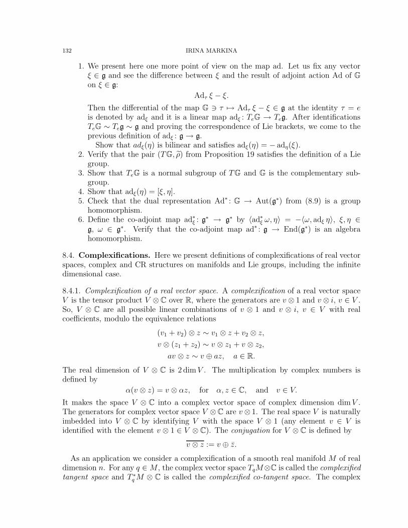
132 IRINA MARKINA
1. We present here one more point of view on the map ad. Let us fix any vectorξ ∈ g and see the difference between ξ and the result of adjoint action Ad of Gon ξ ∈ g:
Adτ ξ − ξ.
Then the differential of the map G $ τ %→ Adτ ξ − ξ ∈ g at the identity τ = eis denoted by adξ and it is a linear map adξ : TeG → Teg. After identificationsTeG ∼ Teg ∼ g and proving the correspondence of Lie brackets, we come to theprevious definition of adξ : g → g.
Show that adξ(η) is bilinear and satisfies adξ(η) = − adη(ξ).2. Verify that the pair (TG, ρ) from Proposition 19 satisfies the definition of a Lie
group.3. Show that TeG is a normal subgroup of TG and G is the complementary sub-
group.4. Show that adξ(η) = [ξ, η].5. Check that the dual representation Ad∗ : G → Aut(g∗) from (8.9) is a group
homomorphism.6. Define the co-adjoint map ad∗ξ : g∗ → g∗ by 〈ad∗ξ ω, η〉 = −〈ω, adξ η〉, ξ, η ∈
g, ω ∈ g∗. Verify that the co-adjoint map ad∗ : g → End(g∗) is an algebrahomomorphism.
8.4. Complexifications. Here we present definitions of complexifications of real vectorspaces, complex and CR structures on manifolds and Lie groups, including the infinitedimensional case.
8.4.1. Complexification of a real vector space. A complexification of a real vector spaceV is the tensor product V ⊗C over R, where the generators are v ⊗ 1 and v ⊗ i, v ∈ V .So, V ⊗ C are all possible linear combinations of v ⊗ 1 and v ⊗ i, v ∈ V with realcoefficients, modulo the equivalence relations
(v1 + v2)⊗ z ∼ v1 ⊗ z + v2 ⊗ z,
v ⊗ (z1 + z2) ∼ v ⊗ z1 + v ⊗ z2,
av ⊗ z ∼ v ⊕ az, a ∈ R.
The real dimension of V ⊗ C is 2 dim V . The multiplication by complex numbers isdefined by
α(v ⊗ z) = v ⊗ αz, for α, z ∈ C, and v ∈ V.
It makes the space V ⊗ C into a complex vector space of complex dimension dim V .The generators for complex vector space V ⊗C are v⊗ 1. The real space V is naturallyimbedded into V ⊗ C by identifying V with the space V ⊗ 1 (any element v ∈ V isidentified with the element v ⊗ 1 ∈ V ⊗ C). The conjugation for V ⊗ C is defined by
v ⊗ z := v ⊕ z.
As an application we consider a complexification of a smooth real manifold M of realdimension n. For any q ∈ M , the complex vector space TqM⊗C is called the complexifiedtangent space and T ∗q M ⊗ C is called the complexified co-tangent space. The complex
GEOMETRY WITH CONSTRAINTS 133
space T ∗q M ⊗C can also be regarded as the complex dual space of TqM ⊗C by definingthe pairing
〈v ⊗ z, ξ ⊕ w〉 := 〈v, ξ〉zw, for v ∈ TqM, ξ ∈ T ∗q M, z, w ∈ C,
for any point q ∈ M . The complexified tangent bundle is T CM = ∪q∈M
(TqM ⊗ C
)and
the complexified co-tangent bundle is T ∗CM = ∪q∈M
(T ∗q M ⊗ C
). A complexified vector
field L on M is a smooth section of T CM , which means that L assigns to each q ∈ M avector Lq ∈ TqM ⊗ C. In any smooth coordinate system
(U,ϕ = (x1, . . . , xn)
)we can
express L as
Lq =
n∑j=1
Lj(q)∂xj ,
where Lj , j = 1, . . . , n are smooth, complex valued functions defined on U ⊂M .If M is complex manifold of complex dimension n, then it is important to distinguish
between the real tangent bundle and the complexified tangent bundle. The real tangentbundle TM corresponds to a smooth manifold M of real dimension 2n. Its fiber TqM isa real vector space and has real dimension 2n. The fiber TqM ⊗ C of the complexifiedtangent bundle is a complex space of complex dimension 2n.
8.4.2. Complex structures. If the real vector space V is of even dimension, then it ispossible to define an almost complex structure J , that is, a map J : V → V , such thatJ2 = − IdV .
Example 16. Let V = TqR2n ∼= Cn. Take the coordinates q = (x1, y1, . . . , xn, yn). Thestandard almost complex structure for TqR2n is defined by setting
(8.10) J(∂xj ) = ∂yj , J(∂yj ) = −∂xj , j = 1, . . . , n,
on the standard basis. Then J extends by linearity to all TqR2n. This almost complexstructure is designed to simulate the multiplication by i =
√−1.The standard almost complex structure J∗ on the co-tangent space T ∗q R2n is the fol-
lowing
J∗(dxj) = −dyj J∗(dyj) = −dxj , j = 1, . . . , n.
An almost complex structure can be defined on a real tangent space of a complexmanifold M by pushing forward the complex structure from Cn up to M via a coordinatechart. For q ∈ M and a holomorphic chart (U, ζ), ζ : U → Cn, we define Jq : TqM → TqMby
(8.11) Jq(L) := dζ(q)ζ−1J(dqζ(L)),
where J in the right hand side is the standard almost complex structure in Cn. Thedefinition implies that if ζ = (z1, . . . , zn), zj = xj + iyj, then Jq(∂xj) = ∂yj and Jq(∂yj ) =−∂xj .
If J is an almost complex structure on a real vector space V , then we can extend itto an almost complex structure JC on the complexification V ⊗ C by setting
JC(v ⊗ z) := J(v)⊗ z, v ∈ V, z ∈ C.
134 IRINA MARKINA
Then
(8.12) JC(w) = JCw, for w ∈ V ⊗ C.
The linear map JC has two eigenvalues i and −i, since J2C = −1. The corresponding
eigen spaces are denoted by V (1,0) and V (0,1). Thus we have
V ⊗ C = V (1,0) ⊕ V (0,1)
from linear algebra. The property (8.12) implies V (1,0) = V (0,1). Let us construct basesfor V (1,0) and V (0,1). First we observe that v and Jv are linearly independent over R inV , since J has no real eigenvalues. Then
(8.13) v1 − iJv1, . . . , vn − iJvnis a basis for the complex n-dimensional vector space V (1,0) and
(8.14) v1 + iJv1, . . . , vn + iJvnis a basis for the complex n-dimensional vector space V (0,1). Remember, that dim V =2n.
Let us see how it works for a complex n-dimensional manifold M . Let (z1, . . . , zq)with zj = xj + iyj be a set of local holomorphic coordinates and the almost complexstructure on TqM , q ∈ M , is given by (8.11). Define the vector fields
∂zj=
1
2(∂xj − i∂yj ) ∂zj
=1
2(∂xj + i∂yj ), j = 1, . . . , n.
Then in view of the above discussions, a basis for T(1,0)q M is given by ∂z1 , . . . , ∂zn
and a basis for T(0,1)q M is given by ∂z1 , . . . , ∂zn. Due to the form of the bases the
spaces T(1,0)q M and T
(0,1)q M received the names holomorphic and antiholomorphic tan-
gent vector spaces. The Hermitian inner product on TqM ⊗ C is defined by declaringthat ∂z1 , . . . , ∂zn , ∂z1, . . . , ∂zn is an orthonormal basis.
Let M now be a real manifold, such that at each q ∈ M the tangent space TqM admitsan almost complex structure Jq : TqM → TqM . Then it leads to the splitting T CM =T (1,0)M ⊕T (0,1)M into the holomorphic and antiholomorphic bundles, and each of themis naturally isomorphic to the real tangent bundle of M , but now they are equipped withanadditional structure Jq. If T (1,0)M is integrable, that is, [T (1,0)M, T (1,0)M ] ⊂ T (1,0)M ,then the pair (M, T (1,0)M) is called the complex manifold.
8.4.3. Lie groups, Lie algebras and complexification. Let us impose the Lie algebra struc-ture on V and see how one can define a complexification g ⊗ C of the Lie algebrag = (V, [·, ·]). All that we need is to define the Lie bracket
(8.15) [v ⊗ α, u⊗ β] := [v, u]⊗ αβ, v, u ∈ g, α, β ∈ C.
Next we consider the relation between the almost complex structure and the Lie algebrastructure. Let G be a Lie group and g be its Lie algebra. Let J : TeG → TeG be analmost complex structure. It determines the splitting TeG⊗ C = g⊗ C = g(1,0) ⊕ g(0,1).If the subspace g(1,0) is a Lie subalgebra of g ⊗ C, then the pair (G, g(1,0)) is called aleft invariant complex structure. This structure is also right invariant, if g(1,0) is adjoint
GEOMETRY WITH CONSTRAINTS 135
invariant with respect to the adjoint action of the group G, or Adτ ξ ∈ g(1,0) for allξ ∈ g(1,0) and τ ∈ G.
We define now a CR-structure on a real manifold N . We follow a scheme, that issuitable for finite and infinite dimensional manifolds. Let TN be the tangent bundle andD be a corank 1 smooth sub-bundle, where an almost complex structure Jq : Dq → Dq
is defined. Let TN ⊗ C be the complexified tangent bundle, then D ⊗ C is a complexcorank 1 smooth sub-bundle, where the splitting D ⊗ C = D(1,0) ⊕ D(0,1) is defined.If [D(1,0), D(1,0)] ⊂ D(1,0), then D(1,0) is called an integrable CR structure and the pair(N, D(1,0)) is an integrable CR manifold.
Example 17. Let N be a real hypersurface in a complex manifold (M, T (1,0)M). Define
D(1,0) = T (1,0)M |N ∩ TM ⊗ C.
Then (N, D(1,0)) is a CR manifold with the CR structure D(1,0) inherited from the com-plex manifold (M, T (1,0)M). The manifolds S3 ⊂ C2, the boundary of the Siegel upperhalf space in C2 have CR structures induced from C2.
A CR manifold is strongly pseudo-convex if [L, L]q /∈ D(1,0)q ⊕ D
(0,1)q for any local
non-vanishing section L of D(1,0).If we have a Lie group G with a Lie algebra g, then a left invariant CR structure is
defined by a splitting h(1,0)⊕h(0,1) of a complex co-rank 1 subspace g⊗C with subalgebras
h(1,0) and h(0,1) = h(1,0). This structure is strongly pseudoconvex if [ξ, ξ] /∈ h(1,0) ⊕ h(0,1)
holds for any non-zero ξ ∈ h(1,0).
Exercises
1. Show that the standard almost complex structure (8.10) in TqR2n is an isometryin R2n.
2. Show that the description of Jq given in (8.11) does not depend on the choiceof coordinate chart. Conclude that the push forward of the standard almostcomplex structure J from Cn to a complex manifold is well defined.
3. Prove (8.12).4. Show that v − iJv ∈ V (1,0) and v + iJv ∈ V (0,1) for any v ∈ V .5. Prove that (8.13) and (8.14) are linearly independent systems.6. Find the dual basis for ∂z1 , . . . , ∂zn , ∂z1 , . . . , ∂zn with respect to the standard
Hermitian product.7. Verify that the Lie bracket defined by (8.15) is C-linear, skew symmetric and
satisfies the Jacobi identity.
8.5. Fiber bundles.
Definition 58. A fiber bundle is a collection (F, E, B, π), where in general F, E, B aretopological spaces and π is a continuous map π : E → B. It can also be written as
F −→ Eπ−→ B or shortly E
π−→ B.
It is required that for any x ∈ E, there is an open neighborhood U ⊂ B of π(x) (which willbe called a trivializing neighborhood) such that π−1(U) is homeomorphic to the product
136 IRINA MARKINA
space F ×U , in such a way that π carries over to the projection onto the second factor.In other words, the following diagram should commute:
π−1(U)
π''
φ!! F × U,
pr2%%!!!!!!!!!!!
U
where the map pr2 : F × U → U is the natural projection on the second coordinateand φ : π−1(U) → F × U is a homeomorphism. The set of all (Ui,φi) is called a localtrivialization of the bundle.
Thus for any b ∈ B, the pre-image π−1(b) is homeomorphic to F and is called thefiber over b. The set B is called the base space, E is the total space and the map π isthe projection map. Every fiber bundle π : E → B is an open map, since projection pr2
is an open map. Therefore, B carries the quotient topology determined by the map π.
Definition 59. A bundle π′ : E ′ → B′ is a sub-bundle of the bundle π : E → B, providedE ′ is a subspace of E, B′ is a subspace of B and π′ = π|E′ : E ′ → B′.
If we speak about smooth fiber bundle, we require that F, E, B are smooth manifoldsand all other maps are smooth. A smooth sub-bundle (F ′, E ′, B, π|E′) of a bundle(F, E, B, π) is a smooth bundle such that the inclusions
jF : F ′ → F, jE : E ′ → E
are smooth.
Definition 60. Let π′ : E ′ → B and π : E → B be two bundles over the same basespace B. A bundle map (bundle morphism) u :
(π′ : E ′ → B
) −→ (π : E → B
)is a map
u : E ′ → E such that π′ = πu. The last equality is the requirement that the followingdiagram commutes
E ′
π′ 00"""
""""
"!! u !! E,
π11#######
B
Definition 61. The fiber product (direct sum or Whitney sum) of two bundles π′ : E ′ →B and π : E → B over B is the bundle Π : E ′ ⊕ E → B, where
E ′ ⊕E = (q′, q) ∈ E ′ × E | π′(q′) = π(q), and Π(q′, q) = π′(q′) = π(q).The fiber Π−1(b) of Π : E ′ ⊕ E → B over b ∈ B is
π′−1(b)× π−1(b) ⊂ E ′ ×E.
8.5.1. Frame bundle. Let (M, gM) be an n-dimensional oriented Riemannian manifold.The frame bundle π : F → M is a fiber bundle, whose total space F consists of collections(q, v1, . . . , vn) ∈ M × (TqM)n such that gM(vi, vj) = δij . An element (q, v1, . . . , vn) is anorthonormal basis of TqM . Sections of the frame bundle are called orthonormal framefields, and they are just assignments to any point q ∈ M of some orthonormal basis(v1, . . . , vn) ∈ TqM . It SO(TqM) is the group of orientation preserving isometries of the
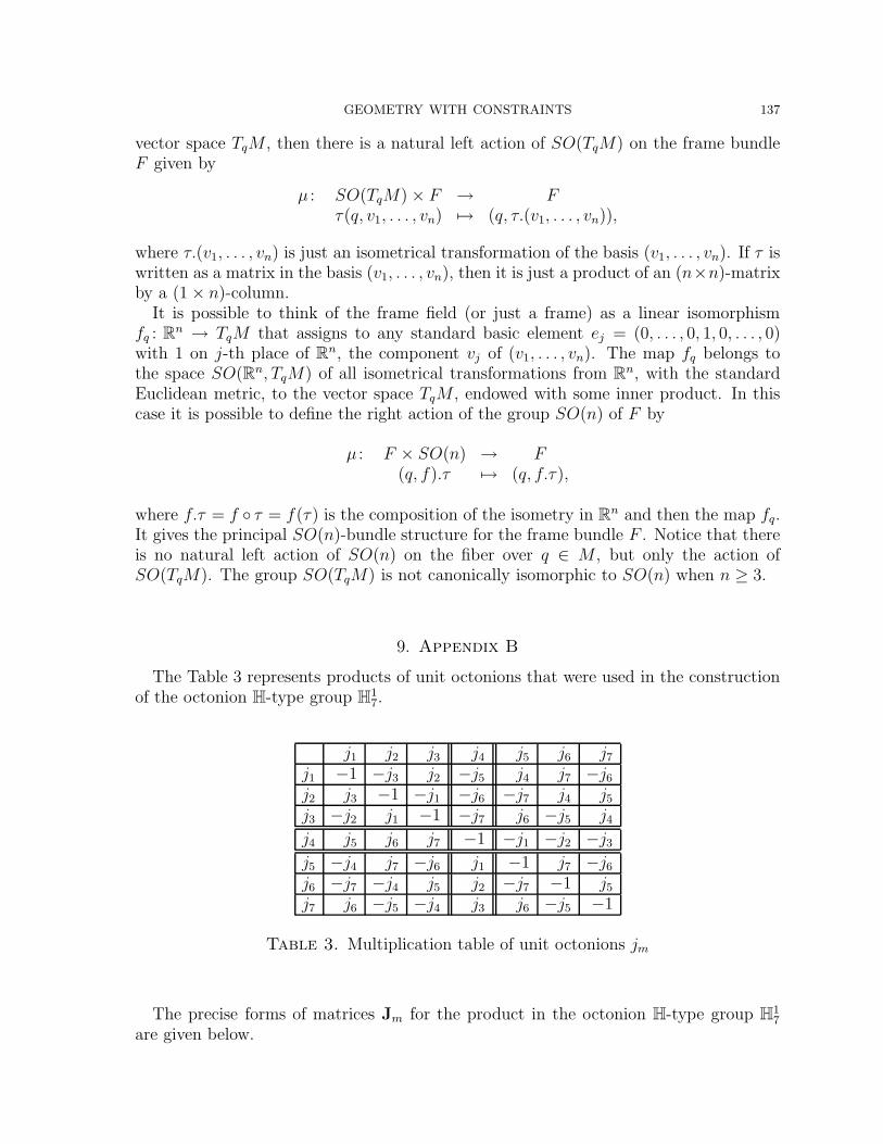
GEOMETRY WITH CONSTRAINTS 137
vector space TqM , then there is a natural left action of SO(TqM) on the frame bundleF given by
µ : SO(TqM)× F → Fτ(q, v1, . . . , vn) %→ (q, τ.(v1, . . . , vn)),
where τ.(v1, . . . , vn) is just an isometrical transformation of the basis (v1, . . . , vn). If τ iswritten as a matrix in the basis (v1, . . . , vn), then it is just a product of an (n×n)-matrixby a (1× n)-column.
It is possible to think of the frame field (or just a frame) as a linear isomorphismfq : Rn → TqM that assigns to any standard basic element ej = (0, . . . , 0, 1, 0, . . . , 0)with 1 on j-th place of Rn, the component vj of (v1, . . . , vn). The map fq belongs tothe space SO(Rn, TqM) of all isometrical transformations from Rn, with the standardEuclidean metric, to the vector space TqM , endowed with some inner product. In thiscase it is possible to define the right action of the group SO(n) of F by
µ : F × SO(n) → F(q, f).τ %→ (q, f.τ),
where f.τ = f τ = f(τ) is the composition of the isometry in Rn and then the map fq.It gives the principal SO(n)-bundle structure for the frame bundle F . Notice that thereis no natural left action of SO(n) on the fiber over q ∈ M , but only the action ofSO(TqM). The group SO(TqM) is not canonically isomorphic to SO(n) when n ≥ 3.
9. Appendix B
The Table 3 represents products of unit octonions that were used in the constructionof the octonion H-type group H1
7.
j1 j2 j3 j4 j5 j6 j7
j1 −1 −j3 j2 −j5 j4 j7 −j6
j2 j3 −1 −j1 −j6 −j7 j4 j5
j3 −j2 j1 −1 −j7 j6 −j5 j4
j4 j5 j6 j7 −1 −j1 −j2 −j3
j5 −j4 j7 −j6 j1 −1 j7 −j6
j6 −j7 −j4 j5 j2 −j7 −1 j5
j7 j6 −j5 −j4 j3 j6 −j5 −1
Table 3. Multiplication table of unit octonions jm
The precise forms of matrices Jm for the product in the octonion H-type group H17
are given below.
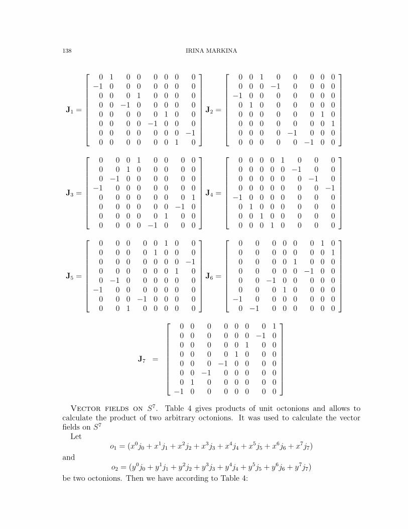
138 IRINA MARKINA
J1 =
0 1 0 0 0 0 0 0−1 0 0 0 0 0 0 0
0 0 0 1 0 0 0 00 0 −1 0 0 0 0 00 0 0 0 0 1 0 00 0 0 0 −1 0 0 00 0 0 0 0 0 0 −10 0 0 0 0 0 1 0
J2 =
0 0 1 0 0 0 0 00 0 0 −1 0 0 0 0−1 0 0 0 0 0 0 0
0 1 0 0 0 0 0 00 0 0 0 0 0 1 00 0 0 0 0 0 0 10 0 0 0 −1 0 0 00 0 0 0 0 −1 0 0
J3 =
0 0 0 1 0 0 0 00 0 1 0 0 0 0 00 −1 0 0 0 0 0 0
−1 0 0 0 0 0 0 00 0 0 0 0 0 0 10 0 0 0 0 0 −1 00 0 0 0 0 1 0 00 0 0 0 −1 0 0 0
J4 =
0 0 0 0 1 0 0 00 0 0 0 0 −1 0 00 0 0 0 0 0 −1 00 0 0 0 0 0 0 −1−1 0 0 0 0 0 0 0
0 1 0 0 0 0 0 00 0 1 0 0 0 0 00 0 0 1 0 0 0 0
J5 =
0 0 0 0 0 1 0 00 0 0 0 1 0 0 00 0 0 0 0 0 0 −10 0 0 0 0 0 1 00 −1 0 0 0 0 0 0
−1 0 0 0 0 0 0 00 0 0 −1 0 0 0 00 0 1 0 0 0 0 0
J6 =
0 0 0 0 0 0 1 00 0 0 0 0 0 0 10 0 0 0 1 0 0 00 0 0 0 0 −1 0 00 0 −1 0 0 0 0 00 0 0 1 0 0 0 0−1 0 0 0 0 0 0 0
0 −1 0 0 0 0 0 0
J7 =
0 0 0 0 0 0 0 10 0 0 0 0 0 −1 00 0 0 0 0 1 0 00 0 0 0 1 0 0 00 0 0 −1 0 0 0 00 0 −1 0 0 0 0 00 1 0 0 0 0 0 0−1 0 0 0 0 0 0 0
Vector fields on S7. Table 4 gives products of unit octonions and allows to
calculate the product of two arbitrary octonions. It was used to calculate the vectorfields on S7
Leto1 = (x0j0 + x1j1 + x2j2 + x3j3 + x4j4 + x5j5 + x6j6 + x7j7)
ando2 = (y0j0 + y1j1 + y2j2 + y3j3 + y4j4 + y5j5 + y6j6 + y7j7)
be two octonions. Then we have according to Table 4:
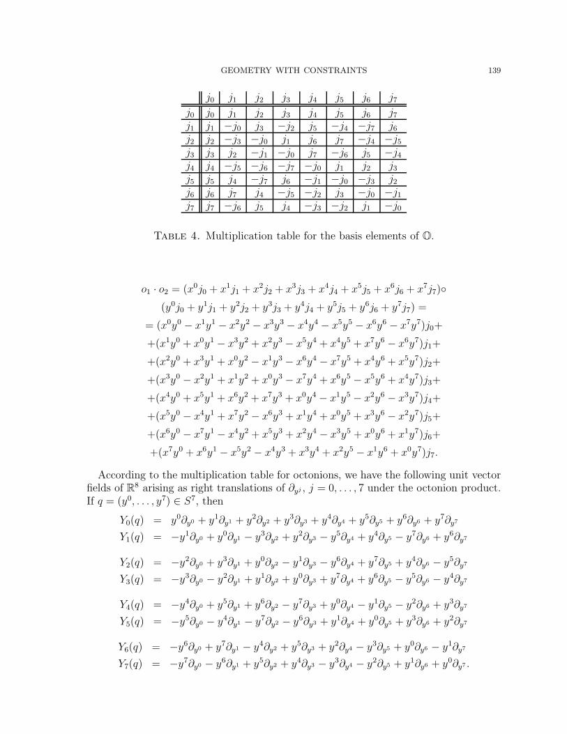
GEOMETRY WITH CONSTRAINTS 139
j0 j1 j2 j3 j4 j5 j6 j7
j0 j0 j1 j2 j3 j4 j5 j6 j7
j1 j1 −j0 j3 −j2 j5 −j4 −j7 j6
j2 j2 −j3 −j0 j1 j6 j7 −j4 −j5
j3 j3 j2 −j1 −j0 j7 −j6 j5 −j4
j4 j4 −j5 −j6 −j7 −j0 j1 j2 j3
j5 j5 j4 −j7 j6 −j1 −j0 −j3 j2
j6 j6 j7 j4 −j5 −j2 j3 −j0 −j1
j7 j7 −j6 j5 j4 −j3 −j2 j1 −j0
Table 4. Multiplication table for the basis elements of O.
o1 · o2 = (x0j0 + x1j1 + x2j2 + x3j3 + x4j4 + x5j5 + x6j6 + x7j7)(y0j0 + y1j1 + y2j2 + y3j3 + y4j4 + y5j5 + y6j6 + y7j7) =
= (x0y0 − x1y1 − x2y2 − x3y3 − x4y4 − x5y5 − x6y6 − x7y7)j0+
+(x1y0 + x0y1 − x3y2 + x2y3 − x5y4 + x4y5 + x7y6 − x6y7)j1+
+(x2y0 + x3y1 + x0y2 − x1y3 − x6y4 − x7y5 + x4y6 + x5y7)j2+
+(x3y0 − x2y1 + x1y2 + x0y3 − x7y4 + x6y5 − x5y6 + x4y7)j3+
+(x4y0 + x5y1 + x6y2 + x7y3 + x0y4 − x1y5 − x2y6 − x3y7)j4+
+(x5y0 − x4y1 + x7y2 − x6y3 + x1y4 + x0y5 + x3y6 − x2y7)j5+
+(x6y0 − x7y1 − x4y2 + x5y3 + x2y4 − x3y5 + x0y6 + x1y7)j6+
+(x7y0 + x6y1 − x5y2 − x4y3 + x3y4 + x2y5 − x1y6 + x0y7)j7.
According to the multiplication table for octonions, we have the following unit vectorfields of R8 arising as right translations of ∂yj , j = 0, . . . , 7 under the octonion product.If q = (y0, . . . , y7) ∈ S7, then
Y0(q) = y0∂y0 + y1∂y1 + y2∂y2 + y3∂y3 + y4∂y4 + y5∂y5 + y6∂y6 + y7∂y7
Y1(q) = −y1∂y0 + y0∂y1 − y3∂y2 + y2∂y3 − y5∂y4 + y4∂y5 − y7∂y6 + y6∂y7
Y2(q) = −y2∂y0 + y3∂y1 + y0∂y2 − y1∂y3 − y6∂y4 + y7∂y5 + y4∂y6 − y5∂y7
Y3(q) = −y3∂y0 − y2∂y1 + y1∂y2 + y0∂y3 + y7∂y4 + y6∂y5 − y5∂y6 − y4∂y7
Y4(q) = −y4∂y0 + y5∂y1 + y6∂y2 − y7∂y3 + y0∂y4 − y1∂y5 − y2∂y6 + y3∂y7
Y5(q) = −y5∂y0 − y4∂y1 − y7∂y2 − y6∂y3 + y1∂y4 + y0∂y5 + y3∂y6 + y2∂y7
Y6(q) = −y6∂y0 + y7∂y1 − y4∂y2 + y5∂y3 + y2∂y4 − y3∂y5 + y0∂y6 − y1∂y7
Y7(q) = −y7∂y0 − y6∂y1 + y5∂y2 + y4∂y3 − y3∂y4 − y2∂y5 + y1∂y6 + y0∂y7 .
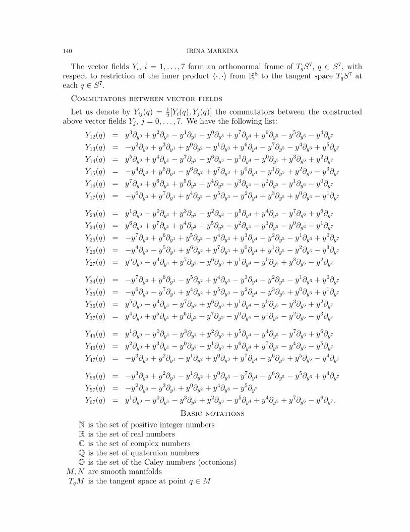
140 IRINA MARKINA
The vector fields Yi, i = 1, . . . , 7 form an orthonormal frame of TqS7, q ∈ S7, with
respect to restriction of the inner product 〈·, ·〉 from R8 to the tangent space TqS7 at
each q ∈ S7.
Commutators between vector fields
Let us denote by Yij(q) = 12[Yi(q), Yj(q)] the commutators between the constructed
above vector fields Yj, j = 0, . . . , 7. We have the following list:
Y12(q) = y3∂y0 + y2∂y1 − y1∂y2 − y0∂y3 + y7∂y4 + y6∂y5 − y5∂y6 − y4∂y7
Y13(q) = −y2∂y0 + y3∂y1 + y0∂y2 − y1∂y3 + y6∂y4 − y7∂y5 − y4∂y6 + y5∂y7
Y14(q) = y5∂y0 + y4∂y1 − y7∂y2 − y6∂y3 − y1∂y4 − y0∂y5 + y3∂y6 + y2∂y7
Y15(q) = −y4∂y0 + y5∂y1 − y6∂y2 + y7∂y3 + y0∂y4 − y1∂y5 + y2∂y6 − y3∂y7
Y16(q) = y7∂y0 + y6∂y1 + y5∂y2 + y4∂y3 − y3∂y4 − y2∂y5 − y1∂y6 − y0∂y7
Y17(q) = −y6∂y0 + y7∂y1 + y4∂y2 − y5∂y3 − y2∂y4 + y3∂y5 + y0∂y6 − y1∂y7
Y23(q) = y1∂y0 − y0∂y1 + y3∂y2 − y2∂y3 − y5∂y4 + y4∂y5 − y7∂y6 + y6∂y7
Y24(q) = y6∂y0 + y7∂y1 + y4∂y2 + y5∂y3 − y2∂y4 − y3∂y5 − y0∂y6 − y1∂y7
Y25(q) = −y7∂y0 + y6∂y1 + y5∂y2 − y4∂y3 + y3∂y4 − y2∂y5 − y1∂y6 + y0∂y7
Y26(q) = −y4∂y0 − y5∂y1 + y6∂y2 + y7∂y3 + y0∂y4 + y1∂y5 − y2∂y6 − y3∂y7
Y27(q) = y5∂y0 − y4∂y1 + y7∂y2 − y6∂y3 + y1∂y4 − y0∂y5 + y3∂y6 − y2∂y7
Y34(q) = −y7∂y0 + y6∂y1 − y5∂y2 + y4∂y3 − y3∂y4 + y2∂y5 − y1∂y6 + y0∂y7
Y35(q) = −y6∂y0 − y7∂y1 + y4∂y2 + y5∂y3 − y2∂y4 − y3∂y5 + y0∂y6 + y1∂y7
Y36(q) = y5∂y0 − y4∂y1 − y7∂y2 + y6∂y3 + y1∂y4 − y0∂y5 − y3∂y6 + y2∂y7
Y37(q) = y4∂y0 + y5∂y1 + y6∂y2 + y7∂y3 − y0∂y4 − y1∂y5 − y2∂y6 − y3∂y7
Y45(q) = y1∂y0 − y0∂y1 − y3∂y2 + y2∂y3 + y5∂y4 − y4∂y5 − y7∂y6 + y6∂y7
Y46(q) = y2∂y0 + y3∂y1 − y0∂y2 − y1∂y3 + y6∂y4 + y7∂y5 − y4∂y6 − y5∂y7
Y47(q) = −y3∂y0 + y2∂y1 − y1∂y2 + y0∂y3 + y7∂y4 − y6∂y5 + y5∂y6 − y4∂y7
Y56(q) = −y3∂y0 + y2∂y1 − y1∂y2 + y0∂y3 − y7∂y4 + y6∂y5 − y5∂y6 + y4∂y7
Y57(q) = −y2∂y0 − y3∂y1 + y0∂y2 + y4∂y6 − y5∂y7
Y67(q) = y1∂y0 − y0∂y1 − y3∂y2 + y2∂y3 − y5∂y4 + y4∂y5 + y7∂y6 − y6∂y7 .
Basic notations
N is the set of positive integer numbersR is the set of real numbersC is the set of complex numbersQ is the set of quaternion numbersO is the set of the Caley numbers (octonions)
M, N are smooth manifoldsTqM is the tangent space at point q ∈ M
GEOMETRY WITH CONSTRAINTS 141
T ∗q M is the cotangent space at point q ∈ MTM is the tangent bundle for a manifold M
T ∗M is the cotangent bundle for a manifold MprM , pr∗M are the canonical projections from TM , T ∗M to M
Vect M is the set of smooth vector fields on MX, Y, Z are smooth vector fields, elements of Vect M
S1 is the unit circleDiff S1 is the group of orientation preserving diffeomorphisms of S1
Vir is the Virasoro-Bott groupvir is the Virasoro algebraD is a smooth distribution on M , horizontal sub-bundle of TM
D∗ is a smooth co-distribution on M , smooth sub-bundle of T ∗MD⊥ is the set of annihilators of D, horizontal sub-bundle of TM
g is a Riemannian metricgD is a sub-Riemannian metric related to the distribution DgD is a sub-Riemannian co-metric related to the distribution DΩ is a curvature form of a horizontal distributionA is a connection form of a horizontal distributionσ is the infinitesimal generator of a group acting on a manifold∇ is the Levi-Civita connectionH is a Hamiltonian function−→H is the Hamiltonian vector field associated to a function H
G, H are Lie groupsg, h are Lie algebras
Aut(E) is the group of automorphisms of EEnd(E) is the the Lie algebra of endomorphisms of EW, W ∗ is a vector space and it dual
· is the Euclidean inner product(·, ·) is an inner product〈·, ·〉 is a pairing between W and W ∗
·, · are Poisson brackets[·, · ] is the commutator
‖ · ‖E is the Euclidean norm‖ · ‖H1 is the Heisenberg norm
dE is the Euclidean distance functiondH1 is the Heisenberg distance functiondc−c is the Carnot-Caratheodory distance functionf |S is the restriction of the function f to the set S
grad f is the Riemannian gradient of a function fgradD f is the sub-Riemannian gradient of a function f
R is the rolling map
References
[1] J. F. Adams, Vector Fields on Spheres, Ann. of Math. (2) 75 (1962) 603–632.
142 IRINA MARKINA
[2] A. Agrachev, M. Caponigro, Controllability on the group of diffeomorphisms, Annales de lInstitutHenri Poincare. Analyse Non Lineaire 26 (2009), 2503–2509.
[3] A. Agrachev, Y. Sachkov, Control theory from the geometric viewpoint, Encyclopaedia of Math-ematical Sciences, 87. Control Theory and Optimization, II. Springer-Verlag, Berlin, 2004. 412pp.
[4] H. Airault, P. Malliavin, Unitarizing probability measures for representations of Virasoro algebra.J. Math. Pures Appl. 80 (2001), no. 6, 627–667.
[5] D. Alekseevsky, Y. Kamishima, Pseudo-conformal quaternionic CR structure on (4n + 3)− di-mensional manifolds. Ann. Mat. Pura Appl. (4) 187 (2008), no. 3, 487–529.
[6] N. Arcozzi, A. Baldi, From Grushin to Heisenberg via an isoperimetric problem. J. Math. Anal.Appl. 340 (2008), no. 1, 165–174.
[7] V. I. Arnold, Mathematical methods of classical mechanics. Translated from the 1974 Russian orig-inal by K. Vogtmann and A. Weinstein. Corrected reprint of the second (1989) edition. GraduateTexts in Mathematics, 60. Springer-Verlag, New York, 516 pp.
[8] J. C. Baez, The octonions. Bull. Amer. Math. Soc. (N.S.) 39 (2002), no. 2, 145–205.[9] W. Bauer, K. Furutani, Spectral analysis and geometry of a sub-Riemannian structure on S3
and S7. J. Geom. Phys. 58 (2008) 1693–1738.[10] M. Bauer, D. Bernard, SLE martingales and the Virasoro algebra. Phys. Lett. B 557 (2003), no.
3-4, 309316,[11] M. Bauer, D. Bernard, Conformal field theories of stochastic Loewner evolutions. Comm. Math.
Phys. 239 (2003), no. 3, 493521.[12] A. Bellaıche. The tangent space in Sub-Riemannian geometry in Sub-Riemannian geometry Edited
by Andre Bellache and Jean-Jacques Risler. Progress in Mathematics, 144. Birkhuser Verlag,Basel, 1996. 393 pp
[13] A. Boggess, CR manifolds and the tangential Cauchy-Riemann complex. Studies in AdvancedMathematics. CRC Press, Boca Raton, FL, 1991. 364 pp.
[14] V. G. Boltyanskii, Sufficient conditions for optimality and the justification of the dynamic pro-gramming method, SIAM J. Control 4 1966 326–361.
[15] R. Bott, On the characteristic classes of groups of diffeomorphisms. Enseignment Math. (2) 23(1977), no. 3-4, 209220.
[16] R. Bott, J. Milnor, On the parallelizability of the spheres. Bull. Amer. Math. Soc. 64 (1958) 87–89.[17] R. Bryant, L. Hsu, Rigidity of integral curves of rank 2 distributions. Invent. Math. 114 (1993),
no. 2, 435–461.[18] O. Calin, D. C. Chang, P. Greiner, Geometric analysis on the Heisenberg group and its gen-
eralizations, AMS/IP Studies in Advanced Mathematics, 40. American Mathematical Society,Providence, RI; International Press, Somerville, MA, 2007. 244 pp.
[19] O. Calin, D. C. Chang, I. Markina, Geometric analysis on H-type groups related to divisionalgebras. Math. Nachr. 282 (2009), no. 1, 44–68.
[20] L. Capogna, D. Danielli, S. D. Pauls, J. T. Tyson. An introduction to the Heisenberg group and thesub-Riemannian isoperimetric problem. Progress in Mathematics, 259. Birkhuser Verlag, Basel,2007. 223 pp.
[21] M. P. do Carmo, Riemannian geometry, Mathematics: Theory & Applications. Birkhuser Boston,Inc., Boston, MA, 1992. 300 pp.
[22] E. Cartan, Les systemes de Pfaff, a cinq variables et les equations aux derivees partielles du secondordre. Ann. Sci. Ecole Norm. Sup. 27 (1910), no. 3, 109–192.
[23] C. H. Chang, D. C. Chang, B. Gaveau, P. Greiner, H. P. Lee, Geometric analysis on a step 2Grusin operator, Bull. Inst. Math. Acad. Sin. (N.S.) 4 (2009), no. 2, 119–188.
[24] D. C. Chang, I. Markina, Geometric analysis on quaternion H-type groups, J. Geom. Anal. 16(2006), no. 2, 266–294.
[25] D. C. Chang, I. Markina, A. Vasiliev, Sub-Lorentzian geometry on anti-de Sitter space, J. Math.Pures Appl. 90 (9) (2008), no. 1, 82-110.
GEOMETRY WITH CONSTRAINTS 143
[26] D. C. Chang, I. Markina, A. Vasiliev, Sub-Riemannian geodesics on the 3-D sphere. ComplexAnal. Oper. Theory 3 (2009), no. 1, 44–68.
[27] D. C. Chang, I. Markina, A. Vasiliev, Modified action and differential operators on the 3-D sub-Riemannian sphere, Asian J. Math. 14 (3) (2010) no. 4, 439–474.
[28] W. L. Chow, Uber Systeme von linearen partiellen Differentialgleichungen erster Ordnung, Math.Ann., 117 (1939), 98–105.
[29] M. Cowling, A. H. Dooley, A. Koranyi, F. Ricci, H-type groups and Iwasawa decompositions, Adv.Math. 87 (1991), no. 1, 1–41.
[30] D. Danielli, N. Garofalo, D. M. Nhieu, Sub-Riemannian calculus on hypersurfaces in Carnotgroups, Adv. Math. 215 (2007), no. 1, 292378.
[31] G. Darboux, Sur le probleme de Pfaff. Bull. Sci. Math. 6 (1882) 14–36, 49–68.[32] J. Dou, P. Niu, J. Han, Polar coordinates for the generalized Baouendi-Grushin operator and
applications, J. Partial Differential Equations 20 (2007), no. 4, 322–336.[33] P. I. Dubnikov, S. N. Samborskii, Controllability criterion for systems in a Banach space (Gen-
eralization of Chow’s theorem), Ukraine Math. J. 32 (1979), no. 5, 649–653.[34] J. J. Duistermaat, J. A. C. Kolk, Lie groups, Universitext. Springer-Verlag, Berlin, 2000. 344 pp.[35] J. Escher, B. Kolev, and M. Wunch, The geometry of a vorticity model equation, arXiv:1010.4844[36] R. Friedrich, W. Werner, Conformal restriction, highest-weight representations and SLE. Comm.
Math. Phys. 243 (2003), no. 1, 105122,[37] R. M. Friedrich, The Global Geometry of Stochastic Lwner Evolutions. arXiv:0906.5328[38] G. Frobenius, Uber die Pfaffsche probleme, J. fur Reine und Agnew. Math 82, (1877) 230–315.[39] G. B. Folland, A fundamental solution for a subelliptic operator. Bull. Amer. Math. Soc. 79 (1973),
373376.[40] G. B. Folland, E. M. Stein, Hardy spaces on homogeneous groups, Mathematical Notes, 28. Prince-
ton University Press, Princeton, N.J.; University of Tokyo Press, Tokyo, 1982. 285 pp.[41] W. Fulton, J. Harris, Representation theory. A first course. Graduate Texts in Mathematics, 129.
Readings in Mathematics. Springer-Verlag, New York, 1991. 551 pp.[42] N. Garofalo, D. Vassilev, Strong unique continuation properties of generalized Baouendi-Grushin
operators, Comm. Partial Differential Equations 32 (2007), no. 4-6, 643–663.[43] Z. Ge, Betti numbers, characteristic classes and sub-Riemannian geometry Illinois J. Math. 36
(1992), no. 3, 372–403.[44] I. M. Gel’fand, D. B. Fuchs, Cohomology of the Lie algebra of vector fields on the circle. Functional
Anal. Appl. 2 (1968), no. 4, 342–343.[45] V. Gershkovich, A. Vershik, Nonholonomic manifolds and nilpotent analysis, J. Geom. Phys. 5
(1988), no. 3, 407–452.[46] M. Godoy Molina, E. Grong,I. Markina, S. Leite, An intrinsic formulation of the rolling manifolds
problem, submitted, arXive 1008.1856[47] M. Godoy, I. Markina, Sub-Riemannian geometry of parallelizable spheres, Matemtica Revista
Iberoamericana 27 (2011),no. 3, 997–1022.[48] M. Godoy, I. Markina, Sub-Riemannian geodesics and heat operator on odd dimensional spheres.
Arxiv 1008.5265[49] M. Grochowski Geodesics in the sub-Lorentzian geometry. Bull. Polish Acad. Sci. Math. 50
(2002), no. 2, 161–178.[50] M. Grochowski Reachable sets for the Heisenberg sub-Lorentzian structure on R3. An estimate
for the distance function. J. Dyn. Control Syst. 12 (2006), no. 2, 145–160.[51] M. Gromov. Carnot-Caratheodory spaces seen from within in Sub-Riemannian geometry Edited by
Andre Bellache and Jean-Jacques Risler. Progress in Mathematics, 144. Birkhuser Verlag, Basel,1996. 393 pp
[52] E. Grong, I. Markina, A. Vasiliev Geometry with non-holonomic constraints on infinite dimen-sional manifolds. Preprint Mittag-Leffler Institute, Stockholm, Sweden.
[53] V. V. Grusin, A certain class of hypoelliptic operators, (Russian) Mat. Sb. (N.S.) 83 (125), (1970),456–473.
144 IRINA MARKINA
[54] E. Heintze, X. Liu, Homogeneity of infinite dimensional isoparametric submanifolds, Annals ofMathematics, 149 (1999), 149–181.
[55] M. R. Herman, Simplicite du groupe des diffeomorphismes de classe C∞, isotopes a l’identite, dutore de dimension n. (French) C. R. Acad. Sci. Paris Ser. A-B 273 1971, A232–A234.
[56] H. Hopf, Uber die Abbildungen von Spharen auf Spharen niedrigerer Dimension. Math. Ann. 104(1931), 637–665.
[57] K. Huper, F. Silva Leite, On the geometry of rolling and interpolation curves on Sn, SOn, andGrassmann manifolds, J. Dyn. Control Syst. 13 (2007), no. 4, 467–502.
[58] K. Huper, M. Kleinsteuber, F. Silva Leite, Rolling Stiefel manifolds, Internat. J. Systems Sci. 39(2008), no. 9, 881–887.
[59] A. Hurtado, C. Rosales, Area-stationary surfaces inside the sub-Riemannian three-sphere, Math.Ann. 340 (2008), no. 3, 675–708.
[60] D. Husemoller, !Fibre bundles, Third edition. Graduate Texts in Mathematics, 20. Springer-Verlag,New York, 1994. 353 pp.
[61] A. Kaplan, Fundamental solutions for a class of hypoelliptic PDE generated by composition ofquadratics forms, Trans. Amer. Math. Soc. 258 (1980), no. 1, 147–153.
[62] A. Kaplan, On the geometry of groups of Heisenberg type, Bull. London Math. Soc. 15 (1983),no. 1, 35–42.
[63] B. Khesin, G. Misio#lek, Euler equations on homogeneous spaces and Virasoro orbits. Adv. Math.176 (2003), no. 1, 116144.
[64] B. Khesin, R. Wendt, The geometry of infinite-dimensional groups. A Series of Modern Surveys inMathematics [Results in Mathematics and Related Areas. 3rd Series. A Series of Modern Surveysin Mathematics], 51. Springer-Verlag, Berlin, 2009. 304 pp.
[65] A. A. Kirillov, The orbits of the group of diffeomorphisms of the circle, and local Lie superalgebras.(Russian) Funktsional. Anal. i Prilozhen. 15 (1981), no. 2, 75–76.
[66] A. A. Kirillov, Geometric approach to discrete series of unirreps for vir, J. Math. Pures Appl. 77(1998) 735–746
[67] A. A. Kirillov, D. V. Yuriev, Representations of the Virasoro algebra by the orbit method, J. Geom.Phys. 5 (3) (1988) 351–363.
[68] A. A. Kirillov, Kahler structures on K-orbits of the group of diffeomorphisms of a circle, Funct.Anal. Appl. 21 (1987), no. 2, 42–45
[69] A. A. Kirillov, D. V. Yur’ev, Kahler geometry and the infinite-dimensional homogenous spaceM = Diff+(S1)/Rot(S1), Funct. Anal. Appl. 21 (1987), no. 4, 284–294.
[70] A. W. Knapp, Lie groups beyond an introduction, Second edition. Progress in Mathematics, 140.Birkhuser Boston, Inc., Boston, MA, 2002. 812 pp.
[71] A. Koranyi, Geometric properties of Heisenberg-type groups, Adv. in Math. 56 (1985), no. 1,28–38.
[72] A. Kornyi, H. M. Reimann, Quasiconformal mappings on the Heisenberg group Invent. Math. 80(1985), no. 2, 309–338.
[73] A. Korolko, I. Markina, Nonholonomic Lorentzian geometry on some H-type groups, J. Geom.Anal. 19 (2009), no. 4, 864–889.
[74] A. Korolko, I. Markina, Geodesics on H-type groups with sub-Lorentzian metric and their physicalinterpretation. Comp. Anal. Oper. Theory. 4 (2010), no. 3, 589–618.
[75] A. Korolko, I. Markina, Semi-Riemannian geometry with nonholonomic constraints,Taiwanese J.of Math., (to appear December 2011) Arxiv 0901.144738.
[76] A. Kriegl, P. W. Michor, The convenient setting of global analysis. Mathematical Surveys andMonographs, 53. American Mathematical Society, Providence, RI, 1997. 618 pp.
[77] Yu. S. Ledyaev, On an infinite-dimensional variant of the Rashevski-Chow theorem. Dokl. Akad.Nauk 398 (2004), no. 6, 735-737.
[78] E. B. Lee, L. Markus, Foundations of optimal control theory, John Wiley & Sons, Inc., NewYork-London-Sydney 1967, 576 pp.
[79] L. Lempert, The Virasoro group as a complex manifold. Math. Res. Lett. 2 (1995), no. 4, 479495.
GEOMETRY WITH CONSTRAINTS 145
[80] W. Liu, H. J. Sussmann, Shortest paths for sub-Riemannian metrics on rank-two distributions,Mem. Amer. Math. Soc. 118 (1995), no. 564, 104 pp.
[81] D. W. Lyons, An elementary introduction to the Hopf fibration. Math. Mag. 76 (2003), no. 2,87-98.
[82] I. Markina, A. Vasil’ev, Virasoro algebra and dynamics in the space of univalent functions. Fivelectures in complex analysis, 85116, Contemp. Math., 525, Amer. Math. Soc., Providence, RI,2010.
[83] I. Markina, A. Vasil’ev, Evolution of smooth shapes and integrable systems. arXiv:1108.1007[84] J. Marsden, A. Weinstein, Reduction of symplectic manifolds with symmetry. Rep. Mathematical
Phys. 5 (1974), no. 1, 121130.[85] K. R. Meyer, Symmetries and integrals in mechanics. Dynamical systems (Proc. Sympos., Univ.
Bahia, Salvador, 1971), pp. 259272. Academic Press, New York, 1973.[86] P. W. Michor, D. Mumford, Riemannian geometries on spaces of plane curves. J. Eur. Math. Soc.
(JEMS) 8 (2006), no. 1, 148.[87] P. W. Michor, D. Mumford, An overview of the Riemannian metrics on spaces of curves using
the Hamiltonian approach. Appl. Comput. Harmon. Anal. 23 (2007), no. 1, 74113.[88] P. W. Michor, D. Mumford, J. Shah, L. Younes, A metric on shape space with explicit geodesics.
Atti Accad. Naz. Lincei Cl. Sci. Fis. Mat. Natur. Rend. Lincei (9) Mat. Appl. 19 (2008), no. 1,2557.
[89] J. Milnor, Morse theory, Annals of Mathematics Studies, No. 51 Princeton University Press,Princeton, N.J. 1963, 153 pp.
[90] J. Milnor, D. Husemoller, Symmetric bilinear forms, Ergebnisse der Mathematik und ihrer Gren-zgebiete, Band 73. Springer-Verlag, New York-Heidelberg, 1973, 147 pp.
[91] J. Milnor, Remarks on infinite-dimensional Lie groups. Relativity, groups and topology, II (LesHouches, 1983), 10071057, North-Holland, Amsterdam, 1984.
[92] R. Montgomery, Abnormal minimizers, SIAM J. Control Optim. 32 (1994), no. 6, 1605–1620.[93] R. Montgomery, A survey of singular curves in sub-Riemannian geometry, J. Dynam. Control
Systems 1 (1995), no. 1, 49–90.[94] R. Montgomery, A tour of subriemannian geometries, their geodesics and applications, Mathe-
matical Surveys and Monographs, 91. American Mathematical Society, Providence, RI, 2002. 259pp.
[95] T. Nagano, Linear differential systems with singularities and an application to transitive Liealgebras. J. Math. Soc. Japan 18 (1966), 398–404.
[96] A. Nagel, E. M. Stein, S. Wainger, Balls and metrics defined by vector fields. I. Basic properties,Acta Math. 155 (1985), no. 1-2, 103–147.
[97] J. Nash, The imbedding problem for Riemannian manifolds. Ann. of Math. 63 (1956), no. 2, 20–63.[98] H. Omori, Infinite-dimensional Lie groups. Translated from the 1979 Japanese original and revised
by the author. Translations of Mathematical Monographs, 158. American Mathematical Society,Providence, RI, 1997. 415 pp.
[99] B. O’Neill Semi-Riemannian geometry. With applications to relativity, Pure and Applied Math-ematics, 103. Academic Press, [Harcourt Brace Jovanovich, Publishers], New York, 1983. 468pp.
[100] A. Pressley, G. Segal, Loop groups. Oxford Mathematical Monographs. Oxford Science Publica-tions. The Clarendon Press, Oxford University Press, New York, 1986. 318 pp.
[101] P. K. Rashevskiı About connecting two points of complete nonholonomic space by admissiblecurve, Uch. Zapiski Ped. Inst. K. Liebknecht 2 (1938), 83–94.
[102] F. Ricci, The spherical transform on harmonic extensions of H-type groups, Differential geometry(Turin, 1992). Rend. Sem. Mat. Univ. Politec. Torino, 50 (1992), no. 4, 381–392.
[103] M. Ritore, A proof by calibration of an isoperimetric inequality in the Heisenberg group Hn,arXiv:0803.1313v3 (to appear in Calc. Var.)
[104] M. Ritore, C. Rosales, Area-stationary and stable surfaces in the sub-Riemannian Heisenberggroup H1, Mat. Contemp. 35 (2008), 185203.
146 IRINA MARKINA
[105] A. A. Sagle, R. E. Walde, Introduction to Lie Groups and Lie Algebras, Pure and Applied Math-ematics, 51. Academic Press, New York-London, 1973. 361 pp.
[106] A. C. Schaeffer, D. C. Spencer, Coefficient Regions for Schlicht Functions (With a Chapter on theRegion of the Derivative of a Schlicht Function by Arthur Grad), American Mathematical SocietyColloquium Publications, Vol. 35. American Mathematical Society, New York, 1950.
[107] R. W. Sharpe, Differential geometry. Cartan’s generalization of Klein’s Erlangen program. Grad-uate Texts in Mathematics, 166. Springer-Verlag, New York, 1997. 421 pp.
[108] I. M. Singer, J. A. Thorpe, Lecture notes on elementary topology and geometry. UndergraduateTexts in Mathematics. Springer-Verlag, New York-Heidelberg, 1976. 232 pp.
[109] R. S. Strichartz, Sub-Riemannian geometry, J. Differential Geom. 24 (1986), 221–263; Correction,ibid. 30 (1989), 595–596.
[110] H. J. Sussmann, Orbits of families of vector fields and integrability of distributions, Trans. Amer.Math. Soc. 180 (1973), 171–188.
[111] J. T. Tyson, Sharp weighted Young’s inequalities and Moser-Trudinger inequalities on Heisenbergtype groups and Grushin spaces, Potential Anal. 24 (2006), no. 4, 357–384.
[112] J. Vick, Homology Theory: An Introduction to Algebraic Topology. Graduate Texts in Mathemat-ics, Vol 145. Springer-Verlag New York, 1994.
[113] F. W. Warner, Foundations of differentiable manifolds and Lie groups. Graduate Texts in Math-ematics, 94. Springer-Verlag, New York-Berlin, 1983. 272 pp.
[114] J. A. Zimmerman, Optimal control of the sphere Sn rolling on En, Math. Control Signals Systems17 (2005), no. 1, 14–37.
Department of Mathematics, University of Bergen, Norway.E-mail address : [email protected]