GEOGRAPHIC INFORMATION SYSTEMS FOR SPATIAL DISEASE …

GEOGRAPHIC INFORMATION SYSTEMS FOR SPATIAL DISEASE CLUSTER

DETECTION, SPATIO-TEMPORAL DISEASE MAPPING, AND HEALTH SERVICE

PLANNING

by

PING YIN

(Under the Direction of Lan Mu and Marguerite Madden)

ABSTRACT

Geographic information systems (GIS) are increasingly recognized as an effective and

efficient tool to deal with geographic questions in health studies. The overarching research

question of this dissertation asks how GIS and spatial analysis can be used to facilitate public

health studies. Three aspects of health studies are included: spatial disease cluster detection,

spatio-temporal disease mapping, and health service planning. New methods or models are

proposed and implemented with GIS in this dissertation to address an important problem in each

of the three aspects.

First, a redesigned spatial scan statistic (RSScan) is proposed to quickly detect disease

clusters in arbitrary shapes. The experimental results indicate that the improved RSScan method

generally has higher power and accuracy than three existing methods for detecting the clusters in

irregular shapes. Second, to explore the spatio-temporal patterns of lung cancer incidence risks in

Georgia between 2000 and 2007, a total of seven hierarchical Bayesian models are developed

and compared at the census tract level using a two-year time period as the temporal unit. The

study shows the northwest region of Georgia has stably elevated lung cancer incidence risks for

all the population groups by race and sex. It also shows that there are strong inverse relationships

between socioeconomic status and lung cancer incidence risk in males and weak inverse

relationships in females in Georgia. Finally, two transportation models that address the modular

capacitated maximal covering location problem (MCMCLP) are proposed and used to optimally

site ambulances for Emergency Medical Services (EMS) Region 10 in Georgia. As a component

of the allocation-location problems for health service planning, spatial demand representation is

discussed and three representation approaches are empirically compared in both problem

complexity and representation error.

Results of this dissertation contribute to the advancement of geospatial analysis in disease

surveillance and health service decision making. Future research could include using GIS and

spatial analysis to improve the accuracy of detected clusters, explore the environmental factors

related to the spatio-temporal patterns of lung cancer incidence risks in Georgia, and integrate

population movement in health service planning.

INDEX WORDS: GIS, Public health, Cluster detection, Disease mapping, Health planning



PLANNING

by

PING YIN

B.E., Tsinghua University, China, 2002

M.E., Tsinghua University, China, 2005

A Dissertation Submitted to the Graduate Faculty of The University of Georgia in Partial

Fulfillment of the Requirements for the Degree

DOCTOR OF PHILOSOPHY

ATHENS, GEORGIA

2012

© 2012

Ping Yin

All Rights Reserved



PLANNING

by

PING YIN

Major Professor: Lan Mu Marguerite Madden Committee: Xiaobai Yao Thomas Jordan John Vena Electronic Version Approved: Maureen Grasso Dean of the Graduate School The University of Georgia August 2012

iv

ACKNOWLEDGEMENTS

Five years’ Ph.D. study in the Department of Geography at the University of Georgia

(UGA) is great experience to me. I am grateful to all of those people who supported and helped

me to finish my dissertation research. First and foremost, my deepest gratitude goes to my major

professors, Dr. Lan Mu and Dr. Marguerite Madden, for their excellent guidance and full

supports. Without their endless input, timely feedbacks, and great inspiration, I cannot have my

research finished today. I really appreciate their dedication and generous help to my research and

other academic activities.

I would thank Dr. John Vena in the Department of Epidemiology and Biostatistics at

UGA for providing me the health data for my research. His invaluable advice from an

epidemiological perspective greatly improves my research.

I would also acknowledge Dr. Xiaobai Yao and Dr. Thomas Jordan for their insightful

advices and suggestions on this research and other academic areas.

I want to thank Dr. Andrew Herod. He made me realize that how important correct

citations are in academic writing.

The institutions that sponsored my research deserve special notice. They are the UGA

research foundation and the UGA graduate school with the dean’s award in social sciences and

the dissertation completion award.

Finally, I deeply thank my parents and my wife, Jing. It is their unconditional love and

endless patience that encourage me to finish my dissertation.

v

TABLE OF CONTENTS

Page

ACKNOWLEDGEMENTS .......................................................................................................... iv

LIST OF TABLES ...................................................................................................................... viii

LIST OF FIGURES ........................................................................................................................ x

CHAPTER

1 INTRODUCTION AND LITERATURE REVIEW .................................................... 1

1.1 Background ....................................................................................................... 1

1.2 Research Objectives .......................................................................................... 6

1.3 Literature Review.............................................................................................. 8

1.4 Dissertation Structure...................................................................................... 12

References ............................................................................................................. 13

2 DETECTING DISEASE CLUSTERS IN ARBITRARY SHAPES WITH A

REDESIGNED SPATIAL SCAN STATISTIC ......................................................... 18

Abstract ................................................................................................................. 19

2.1 Introduction ..................................................................................................... 20

2.2 Existing Methods for Detection of Disease Clusters ...................................... 21

2.3 Redesigned Spatial Scan Method (RSScan) ................................................... 24

2.4 Performance Evaluation .................................................................................. 28

2.5 Application: Georgia Lung Cancer, 1998 -2005 ............................................. 37

2.6 Discussion and Conclusions ........................................................................... 38

vi

References ............................................................................................................. 41

3 HIERARCHICAL BAYESIAN MODELING OF THE SPATIO-TEMPORAL

PATTERNS OF LUNG CANCER INCIDENCE RISKS IN GEORGIA, 2000-2007 44

Abstract ................................................................................................................. 45

3.1 Introduction ..................................................................................................... 46

3.2 Study Area and Data ....................................................................................... 48

3.3 Methods........................................................................................................... 50

3.4 Results ............................................................................................................. 57

3.5 Discussions ..................................................................................................... 67

3.6 Conclusions ..................................................................................................... 68

References ............................................................................................................. 70

4 MODULAR CAPACITATED MAXIMAL COVERING LOCATION PROBLEM

FOR THE OPTIMAL SITING OF EMERGENCY VEHICLES ............................... 73

Abstract ................................................................................................................. 74

4.1 Introduction ..................................................................................................... 75

4.2 Modular Capacitated Maximal Covering Location Problem (MCMCLP) ..... 78

4.3 Spatial Demand Representation ...................................................................... 84

4.4 Applications: Optimal Siting of Ambulances ................................................. 85

4.5 Discussion ....................................................................................................... 96

4.6 Conclusion ...................................................................................................... 98

References ............................................................................................................. 99

5 AN EMPIRICAL COMPARISON OF SPATIAL DEMAND REPRESENTATIONS

IN MAXIMAL COVERAGE MODELING ............................................................. 102

vii

Abstract ............................................................................................................... 103

5.1 Introduction ................................................................................................... 104

5.2 Representation Error in Covering Location Modeling ................................. 106

5.3 The MCLP Model and Problem Complexity ................................................ 110

5.4 Service Area Spatial Demand Representation .............................................. 112

5.5 Experimental Design ..................................................................................... 117

5.6 Results and Discussions ................................................................................ 120

5.7 Conclusions ................................................................................................... 130

References ........................................................................................................... 133

6 CONCLUSIONS....................................................................................................... 136

6.1 Summary and Conclusions ........................................................................... 136

6.2 Future Research ............................................................................................ 139

References ........................................................................................................... 142

APPENDICES

I LIST OF ACRONYMS ............................................................................................ 143

viii

LIST OF TABLES

Page

Table 2.1: Test statistics and search strategies of four spatial scan methods ............................... 25

Table 2.2: Information of simulated cluster models ..................................................................... 31

Table 2.3: Estimated power of four spatial scan methods (significance level=0.05) ................... 33

Table 2.4: Contingency table for detected cluster estimates and true clusters ............................. 34

Table 2.5: KIAs between the most likely clusters and true clusters for four spatial scan methods 36

Table 2.6: Average Type I error of four spatial scan methods ..................................................... 37

Table 3.1: Total number of cases of individuals over 20 years old and the percentage of included

cases in the analyses by sex and race ........................................................................... 49

Table 3.2: Variables incorporated in the modified Darden-Kamel Composite Index .................. 51

Table 3.3: Components of logarithms of RRs in the seven Bayesian spatio-temporal models .... 54

Table 3.4: DICs of the seven models ............................................................................................ 57

Table 3.5: Posterior median (95% CI) of the shared temporal components and differential

temporal components ................................................................................................... 66

Table 3.6: Posterior median (95% CI) of the RRs for SES quintile ............................................. 67

Table 3.7: Correlations between the posterior median RRs using model 2 with two different

types of hyperpriors ..................................................................................................... 67

Table 4.1: Information for roads ................................................................................................... 89

Table 4.2: Count of the facilities with varied numbers of ambulances ........................................ 96

Table 5.1: Numbers of demand objects in 45 SASDRs .............................................................. 121

ix

Table 5.2: Numbers of demand objects in all demand representations for comparison ............. 124

Table 5.3: Minimum numbers of facilities reported by models for covering 100% demand ..... 125

Table 5.4: Cost and optimality errors between grid-point-based demand representations and

SASDRs ...................................................................................................................... 127

Table 5.5: Cost and optimality errors between grid-rectangle-based demand representations and

SASDRs ...................................................................................................................... 128

x

LIST OF FIGURES

Page

Figure 1.1: GIS functions and GIS applications in public health ................................................... 4

Figure 1.2: Logical structure of the dissertation research ............................................................... 9

Figure 2.1: Graph-based representation of a region map .............................................................. 27

Figure 2.2: Population 2000 by counties in GA in the United States ........................................... 30

Figure 2.3: Locations of simulated clusters: (a) circular shape (b) linear shape (c) trifurcate shape 30

Figure 2.4: Estimated average power of four spatial scan methods ............................................. 34

Figure 2.5: Average KIAs of four spatial scan methods ............................................................... 36

Figure 2.6: SIRs and the detected cluster of lung cancer incidence in GA, 1998-2005 ............... 38

Figure 3.1: Population density by census tract and the 10 most populous cities in Georgia 2000 48

Figure 3.2: Quintile map of SES in Georgia 2000 ........................................................................ 52

Figure 3.3: Maps of crude standardized incidence ratios (SIRs) by race and sex during 2000-

2001 ............................................................................................................................. 58

Figure 3.4: Maps of the posterior median RRs for white males in each time period ................... 60

Figure 3.5: Maps of the posterior median RRs for white females in each time period ................ 61

Figure 3.6: Maps of the posterior median RRs for black males in each time period .................... 62

Figure 3.7: Maps of the posterior median RRs for black females in each time period ................ 63

Figure 3.8: Maps of elevated RR frequency by race and sex during 2000-2007 .......................... 64

Figure 3.9: Maps of the posterior median of the shared spatial component and differential spatial

components ................................................................................................................. 65

xi

Figure 4.1: Illustration of three demand types: unallocated demand (da and db), covered allocated

demand (dc), and uncovered allocated demand (dd) .................................................... 78

Figure 4.2: Example of the SASDR with circular facility service area (a) demand space U (the

square) and two potential service areas S1 and S2 (the circles) (b) four demand objects

in the SASDR result of demand space U partitioned by service areas S1 and S2 ........ 85

Figure 4.3: Population density of Georgia EMS Region 10 (study area) by census block group

and existing ambulance facility locations ................................................................... 87

Figure 4.4: Road network in EMS Region 10 in GA .................................................................... 89

Figure 4.5: Eight-minute service areas (non-white polygons) of all potential ambulance facility

sites (red points) based on the road network ............................................................... 90

Figure 4.6: SASDR result for the study area with demand (population) distribution .................. 92

Figure 4.7: Results of the MCMCLP models siting 58 ambulances in 82 potential facility

locations with w= 8106 −× (the facility location is rendered in the same color as its

allocation area) (a) the MCMCLP-NFC model (b) the MCMCLP-FC model with 20

facilities ....................................................................................................................... 95

Figure 5.1: Examples of spatial demand representations with (a) census blocks or their centroids,

and (b) rectangle grid or its centroids ....................................................................... 108

Figure 5.2: Illustration of overlay operation A▲B: (a) set A and set B (b) the result from A▲B 114

Figure 5.3: The SASDR with circular facility service area: (a) demand space U and two potential

service areas S1 and S2, (b) the partition of demand space U with service area S1, and

(c) the partition of demand space U with both service areas S1 and S2 ..................... 116

Figure 5.4: Three modes of potential facility sites: (a) regular grid points with spacing R, (b)

centroids of census blocks, and (c) intersections of major roads .............................. 118

xii

Figure 5.5: Examples of grid-point-based and grid- rectangle-based demand representations for

comparison with SASDR .......................................................................................... 120

Figure 5.6: Relationship between Site-Service Index and demand object density in SASDR with

circular service coverage ........................................................................................... 123

Figure 5.7: Percentages of covered demand reported by the MCLP models with 3 types of

demand representations when the configuration of potential facility sites include: (a) 66

grid points, (b) 272 grid points (c) 66 block centroids, and (d) 272 block centroids ..... 126

1

CHAPTER 1

INTRODUCTION AND LITERATURE REVIEW

1.1 Background

Because all fields are changing all along, the debate on the definitions and scopes of

subfields such as “medical geography”, “health geography” and “spatial epidemiology” still

continues (Brown et al. 2010). However, it cannot be denied that more and more attention from

the researchers in health, geography, and other fields are drawn to the geographic component of

health, i.e., the question “where”. Where are populations at risk? Where are hotspot areas with

elevated disease risks? Where can we intervene to eliminate or reduce disease risks? Where can

we locate healthcare facilities to improve health services delivery? Geographic information

systems (GIS), which were originally used within the formal discipline of geography, are

increasingly recognized as an effective and efficient tool to deal with these geographic questions

in research and practices in epidemiology and public health (Rushton 2003, Najafabadi 2009,

Nykiforuk and Flaman 2011, Cromley and McLafferty 2012).

Actually, over 150 years ago, early public health professionals learned that maps could be

used to explore patterns of diseases and relationships between diseases and risk factors. In 1840,

Robert Cowan used a map to show the relationship between fever and overcrowding in Glasgow

(Melnick 2002). The famous story about John Snow, one of the fathers of modern epidemiology,

is often used in current textbooks in epidemiology, disease mapping and GIS to illustrate the one

of the first uses of a map to identify a disease source (Melnick 2002, Koch 2005, Longley et al.

2

2005). In 1854, John Snow plotted a map showing the cholera deaths in the Soho district of

London, by which he demonstrated the association between these deaths and contaminated water

supplies from a public water pump in the center of the outbreak.

Since the development of the first real GIS, the Canada Geographic Information System

in the mid-1960s, there has been a rapid increase and great improvement in the functions of GIS

based on the advances in computer science, cartography, computational geometry, and spatial

statistics. Cromley and McLafferty (2012) define GIS as computer-based systems for the

integration and analysis of geographic data. They classify GIS functions into three broad

categories based on what people want to do with spatial data: 1) spatial database management; 2)

visualization and mapping; and 3) spatial analysis. In the past, GIS was regarded as a technology

as discussed above. Nowadays, GIS has been attached with multiple labels, such as GIS software,

GIS data, GIS community, and doing GIS (Longley et al. 2005). Goodchild (1992) coined the

term of “GIScience” that refers to the research field about the fundamental principles and

questions underlying the activities of using GIS as a technology.

Nykiforuk and Flaman (2011) reviewed GIS applications in public health and classified

four content categories in order of descending prevalence in the literature: disease surveillance,

risk analysis, health access and planning, and community health profiling. Disease surveillance is

the compilation and tracking of data on the incidence prevalence, and spread of disease (Wall

and Devine 2000). Cluster detection, disease mapping, and disease modeling are several

interrelated components of disease surveillance. Cluster detection is an analysis process that aims

to identify hotspot areas with elevated disease risks. Disease mapping is used to understand the

distribution of disease or disease risk in the past or present. Disease modeling extends the disease

mapping to identify factors associated with disease risks in order to predict the future spread of

3

disease. These components of disease surveillance that are important for disease prevention and

control can be conducted in spatial or spatio-temporal dimensions. Risk analysis includes some

aspect(s) of risk – assessment, management, communication, or monitoring – relative to impacts

on health (Nykiforuk and Flaman 2011). Health access and planning is to evaluate and improve

health services delivery. Community health profiling is the compilation of mapping of

information regarding the health of a population in a community. These four categories are

overlapping. For example, in a disease mapping application, risk analyses could also be

conducted.

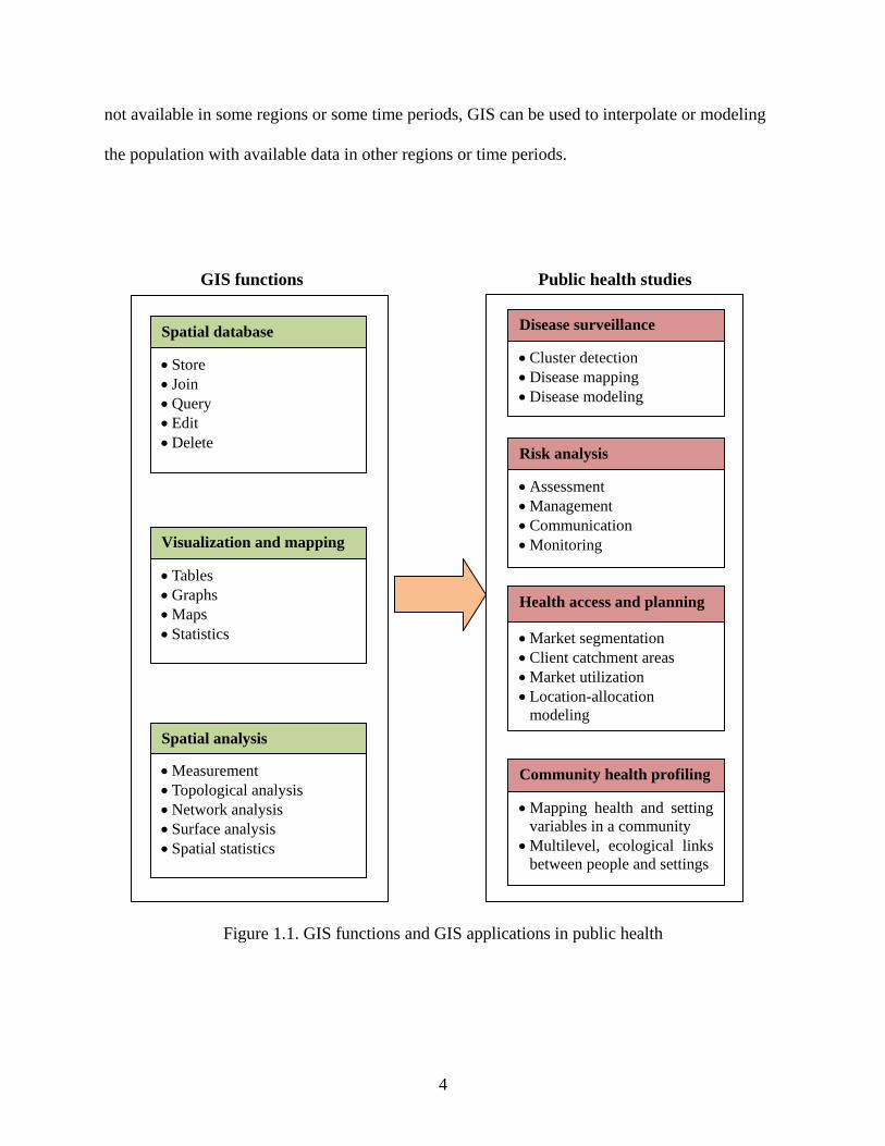
Figure 1.1 shows GIS functions and GIS applications in public health based on Cromley

and McLafferty’s (2012) and Nykiforuk and Flaman’s (2011) classifications discussed above. It

is impossible to completely describe all of GIS functions and how they can be used in public

health studies because the use of GIS functions is usually application-dependent and both GIS

and health studies are evolving all along. Here, we only briefly list several aspects to show how

GIS can greatly facilitate health studies, including population estimation, data integration,

exposure assessment, healthcare access evaluation, and communication.

(1) Population estimation

It is important for health studies to understand the distribution of a population at risk.

Because of the economic and social processes that structure residential development, age, sex

and race-ethnicity of the population are usually not uniform throughout the region of settlement

(Cromley and McLafferty 2012). GIS makes it possible to view residential distributions in great

detail. In addition to residence, GIS can help to model people’s activity in space and their

migration processes to understand the exposure people experienced, which is important for the

studies of diseases with a long latency period such as cancers. Sometimes, population data are

4

not available in some regions or some time periods, GIS can be used to interpolate or modeling

the population with available data in other regions or time periods.

Figure 1.1. GIS functions and GIS applications in public health

Spatial database

• Store • Join • Query • Edit • Delete

Visualization and mapping

• Tables • Graphs • Maps • Statistics

Spatial analysis

• Measurement • Topological analysis • Network analysis • Surface analysis • Spatial statistics

Disease surveillance

• Cluster detection • Disease mapping • Disease modeling

Risk analysis

• Assessment • Management • Communication • Monitoring

Health access and planning

• Market segmentation • Client catchment areas • Market utilization • Location-allocation

modeling

Community health profiling

• Mapping health and setting variables in a community

• Multilevel, ecological links between people and settings

Public health studies GIS functions

5

(2) Data integration

The strong capability of spatial data management of GIS makes it easy to integrate

multiple geographic data of health outcomes and environmental, socioeconomic, and behavioral

factors based on geographic information (location). These spatial data may be collected by

different local, state, or federal agencies, public and private, using different devices or

technology. Linking all of these data can give a more comprehensive context or settings of the

disease of interest, which is essential to identify relationships between diseases and all kinds of

factors and develop etiological hypotheses.

(3) Exposure assessment

Accurate estimation and mapping of exposures is clearly vital if valid inferences are to be

drawn either about the spatial distribution of risk factors, or about their geographic relationship

with health outcome (Elliott et al. 2000). Suitable measures, such as biomarkers, tend to be

costly and invasive. Therefore, especially for population-based research, it is common to

estimate exposure based on environmental monitoring data, such as air pollutant concentrations,

or using proxy measures of exposure, such as distance from source. These indirect methods can

be easily conducted in GIS using interpolation methods and measuring functions.

(4) Healthcare access evaluation

Evaluating current status of health service delivery is important for health policy making

and utilization of resources. The network analysis functions in GIS provide convenient ways to

calculate client catchment areas of healthcare facilities and the shortest distance from population

to healthcare facilities. Some measures for healthcare accessibility, such as the two-step floating

catchment area method (2SFCA) for assessing the local availability of services in relation to

6

population need (Luo and Wang 2003), can easily be implemented in GIS using join and sum

functions.

(5) Communication

Preparing and displaying maps of health information are among the most important

functions of public health GIS (Cromley and McLafferty 2012). By portraying the results of

analysis on a map, GIS technology gives communities an easily understandable visual picture of

community health (Melnick 2002). Maps are recognized as one of the most important

communication tools among researchers, decision makers, and public. With the development of

Internet GIS, the health information can be quickly published using interactive web mapping to

anyone with access to the Internet (Theseira 2002, Boulos 2003, Boulos 2005).

Based on the above examples of GIS applications in health, we can see that GIS can be

used as a natural and effective means to approach a variety of program, policy, and planning

issues in health promotion and public health (Nykiforuk and Flaman 2011).

1.2 Research Objectives

The overarching research question of this dissertation asks how GIS and spatial analysis

can be used to facilitate public health studies. Understanding health status and then effectively

and efficiently providing health care service are necessary to promote public health. Therefore,

this research involves three aspects of health studies related with heath surveillance and health

service planning: spatial disease cluster detection, spatio-temporal disease mapping, and optimal

siting of health facilities. The first two are both techniques used to describe the distribution of a

disease. Spatial disease cluster detection is to quickly identify the hotspot areas with elevated

risks. Usually, it only requires health outcome data and basic population data. It is very useful for

health departments to maintain surveillances on disease outbreaks. However, it cannot provide

7

detailed information on the spatial patterns of disease risks within hotspot areas and other areas

of interest. Spatio-temporal disease mapping can complement cluster detection analysis. It can

provide the spatio-temporal patterns of disease risks across the whole study area and the time

period. These health patterns can be linked to all kinds of factors to develop etiological

hypotheses. Knowing the patterns of disease risks is not the end. The goal of health study is to

prevent and control the spread of disease and promote public health. Given the patterns of

disease risks obtained from disease mapping analyses, we can easily identify areas with high

health service needs. Then, based on the spatial distribution of the needs, health service can be

planned more effectively and efficiently.

This dissertation research includes three main objectives, each of which addresses an

important problem in the three aspects of health studies by developing new methods or models

that are implemented with GIS and spatial analysis. More specifically, these three objects are:

(1) To develop a new method to detect disease clusters in arbitrary shapes with higher

statistical power and more accurate geographic boundaries;

(2) To develop hierarchical Bayesian models to explore the spatio-temporal patterns of

lung cancer incidence risks by race and sex in Georgia (2000-2007) at a fine spatio-temporal

scale;

(3) To develop a new location-allocation model to optimally site ambulances so that the

emergency medical services (EMS) can be delivered more effectively and efficiently.

In the study of the location-allocation model for health service planning, a sub-problem –

spatial demand representation – is worth discussing since it is highly related to modeling errors

and problem complexity. Therefore, this dissertation research is also to empirically compare

8

three existing spatial demand representation approaches to provide some implications on how to

choose appropriate one for a specific application.

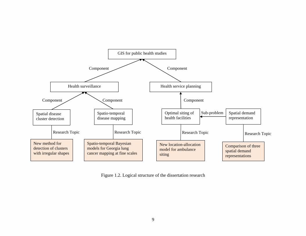
In general, Figure 1.2 shows the logical structure of the dissertation research.

1.3 Literature Review

1.3.1 Detection of Irregular Disease Clusters

Detection of disease clusters in time, space or space-time has generated considerable

interests within disciplines of geography and public health for many decades (Besag and Newell

1991, Maheswaran and Craglia 2004, Lawson 2006). The shape of the geographic area of a true

disease cluster may be arbitrary. For example, air pollution diffusing from an incinerator may

cause an arbitrary disease cluster due to the wind strength and direction. To detect clusters in

irregular shapes, several methods have been proposed in (Duczmal and Assunção 2004, Tango

and Takahashi 2005, Aldstadt and Getis 2006, Duczmal et al. 2006, Kulldorff et al. 2006,

Yiannakoulias et al. 2007, Duczmal et al. 2008, Duczmal et al. 2009, Cançado et al. 2010).

Seeking methods for detection of clusters in irregular shapes with higher statistical power and

more accurate geographic boundary is still a hot topic in current health research.

1.3.2 Spatio-temporal Mapping of Disease Risks

Lung cancer is not only the second most commonly diagnosed cancer in men and women,

but also the leading cause of cancer-related death in Georgia (Georgia Department of Public

Health 2008). However, as far as we know, the lung cancer studies in Georgia are very few, and

most of them mainly focus on descriptive analyses using crude rates at a coarse spatio-temporal

scale, such as the 5-year incidence rates at the health district or county level. Such analyses are

not useful for assessing the health of diverse communities, and could introduce inferential biases

on etiological hypotheses. In addition, they can only provide limited help for healthcare

9

Figure 1.2. Logical structure of the dissertation research

Health surveillance Health service planning

Spatial disease cluster detection

Spatio-temporal disease mapping

Optimal siting of health facilities

New method for detection of clusters with irregular shapes

Spatio-temporal Bayesian models for Georgia lung cancer mapping at fine scales

New location-allocation model for ambulance siting

Spatial demand representation

Comparison of three spatial demand representations

GIS for public health studies

Sub-problem

Component Component

Component Component Component

Research Topic Research Topic Research Topic Research Topic

10

performance assessment and health policy making to improve the efficiency of interventions and

the distribution of resources. The low reliability of the disease rates for small population areas is

one of the challenges for mapping disease risk at a fine spatio-temporal scale. Recently,

hierarchical Bayesian models have been widely used to map disease risk spatially or spatio-

temporally to overcome or mitigate the small number problem (Bernardinelli et al. 1995, Waller

et al. 1997, Xia and Carlin 1998, Knorr-Held 2000, Mollié 2001, Wakefield et al. 2001, Best et

al. 2005, Richardson et al. 2006, Abellan et al. 2008, Lawson 2009, Fortunato et al. 2011).

When mapping one disease for multiple population groups or multiple diseases that have

common risk factors, a joint modeling framework can be used (Knorr-Held and Best 2001, Held

et al. 2005, Richardson et al. 2006, Downing et al. 2008). In this modeling framework, a set of

shared random components exists in each model.

1.3.3 Capacitated Maximal Covering Location Problems

Given a covering standard for a service, such as a distance or travel-time maximum, the

objective of the maximal covering location problem (MCLP) is to locate a fixed number of

facilities to provide the service to cover as many demands as possible. MCLP modeling, after

being put forward by Church and ReVelle (1974), has been a powerful and widely used tool in

many planning processes to optimally distribute limited resources to maximize social and

economic benefits. Chung et al. (1983) and Current and Storbeck (1988) published two early

papers dealing with the capacitated versions of the MCLP where the demands allocated to a

facility will not exceed the capacity of that facility. In all capacitated MCLP models, only one

fixed capacity level of the facility is considered for each potential facility site. However, many

situations arise where each potential facility site could have several possible maximum capacity

levels for a facility to choose. For example, the capacity limit of an emergency facility (e.g.,

11

ambulance base or fire station) can be assumed to be determined by its stationed emergency

vehicles (e.g., ambulances or fire trucks). Therefore, varied numbers of emergency vehicles will

provide a series of possible maximum capacity levels for the emergency facility to choose.

1.3.4 Spatial Demand Representations

For covering location modeling, it is common to assume that aggregated or continuous

spatial demand is concentrated on a set of points or uniformly distributed within areal units.

Different from the traditional area-based representations using census units or regular polygons,

such as triangles or rectangles, as demand objects, Cromley et al. (2012) proposed a new area-

based demand representation that partitions a continuous demand space into a set of the least

common demand coverage units (LCDCUs) by overlaying demand coverage areas at potential

facility sites. This representation approach, without complicated model formulations, could

reduce or eliminate some errors associated with the traditional point-based and area-based

representations.

Many covering location models, such as the maximal covering location problem (MCLP),

have been proven to be nondeterministic polynomial time (NP)-hard (Megiddo et al. 1981),

which means that no algorithm has been discovered yet to solve it in polynomial time in the

worst case. Actually, the size of a covering location problem is highly related to the demand

representation it adopts. Therefore, even if a demand representation approach may theoretically

reduce or eliminate some representation errors in a problem, it probably could make the problem

difficult, if not impossible, to solve using exact methods in current optimization software.

Relying on some heuristic algorithms to solve such a complicated problem may introduce other

errors in modeling results. It is worth noting that the complexity of problems associated with

demand representations is rarely discussed in current literature.

12

1.4 Dissertation Structure

The dissertation structure is organized into six chapters. Chapter 1 is a brief introduction

of the background and objectives of the dissertation research, and literature review of the topics

covered in this dissertation, including the detection of irregular disease cluster, spatio-temporal

mapping of disease risks, capacitated maximal covering location problems, and spatial demand

representations. The following four chapters are separate papers published in or to be submitted

to journals. In Chapter 2, a redesigned spatial scan statistic is proposed to detect disease clusters

with irregular shapes. Chapter 3 develops seven hierarchical Bayesian models under separate and

joint modeling frameworks to explore the spatio-temporal patterns of lung cancer incidence risks

in Georgia (2000-2007) at the census tract level with a two-year temporal unit. Chapter 4

develops modular capacitated maximal covering location problem (MCMCLP) models to

optimally site emergency vehicles (e.g. ambulance). In Chapter 5, three spatial demand

representation approaches are compared in both representation error and problem complexity

using the MCLP as an example. Chapter 6 provides conclusions of this dissertation and shows

the future work.

13

References

Abellan, J.J., Richardson, S. & Best, N., 2008. Use of space–time models to investigate the stability of patterns of disease. Environmental health perspectives, 116 (8), 1111.

Aldstadt, J. & Getis, A., 2006. Using amoeba to create a spatial weights matrix and identify spatial clusters. Geographical analysis, 38 (4), 327-343.

Bernardinelli, L., Clayton, D., Pascutto, C., Montomoli, C., Ghislandi, M. & Songini, M., 1995. Bayesian analysis of space—time variation in disease risk. Statistics in Medicine, 14 (21 22), 2433-2443.

Besag, J. & Newell, J., 1991. The detection of clusters in rare diseases. Journal of the Royal Statistical Society. Series A (Statistics in Society), 154 (1), 143-155.

Best, N., Richardson, S. & Thomson, A., 2005. A comparison of bayesian spatial models for disease mapping. Statistical Methods in Medical Research, 14 (1), 35.

Boulos, M.N.K., 2003. The use of interactive graphical maps for browsing medical/health internet information resources. International Journal Of Health Geographics, 2 (1), 1.

Boulos, M.N.K., 2005. Web gis in practice iii: Creating a simple interactive map of england's strategic health authorities using google maps api, google earth kml, and msn virtual earth map control. International Journal Of Health Geographics, 4 (1), 22.

Brown, T., Mclafferty, S. & Moon, G. eds. 2010. A companion to health and medical geography, Chichester, UK: Wiley-Blackwell.

Cançado, A.L.F., Duarte, A.R., Duczmal, L.H., Ferreira, S.J., Fonseca, C.M. & Gontijo, E.C.D.M., 2010. Penalized likelihood and multi-objective spatial scans for the detection and inference of irregular clusters. International Journal of Health Geographics, 9 (1), 55.

Chung, C., Schilling, D. & Carbone, R., Year. The capacitated maximal covering problem: A heuristiced.^eds. Proceedings of the Fourteenth Annual Pittsburgh Conference on Modeling and Simulation, 1423-1428.

Church, R. & Revelle, C., 1974. The maximal covering location problem. Papers in regional science, 32 (1), 101-118.

14

Cromley, E.K. & Mclafferty, S.L., 2012. Gis and public health, 2nd ed. New York: The Guilford Press.

Cromley, R.G., Lin, J. & Merwin, D.A., 2012. Evaluating representation and scale error in the maximal covering location problem using gis and intelligent areal interpolation. International Journal of Geographical Information Science, 26 (3), 495-517.

Current, J. & Storbeck, J., 1988. Capacitated covering models. Environment and Planning B, 15, 153-164.

Downing, A., Forman, D., Gilthorpe, M., Edwards, K. & Manda, S., 2008. Joint disease mapping using six cancers in the yorkshire region of england. International Journal of Health Geographics, 7 (1), 41.

Duczmal, L. & Assunção, R., 2004. A simulated annealing strategy for the detection of arbitrarily shaped spatial clusters. Computational Statistics & Data Analysis, 45 (2), 269-286.

Duczmal, L., Cançado, A.L.F. & Takahashi, R.H.C., 2008. Geographic delineation of disease clusters through multi-objective optimization. Journal of Computational & Graphical Statistics, 17, 243-262.

Duczmal, L., Duarte, A.R. & Tavares, R., 2009. Extensions of the scan statistic for the detection and inference of spatialclusters. Scan Statistics, 153-177.

Duczmal, L., Kulldorff, M. & Huang, L., 2006. Evaluation of spatial scan statistics for irregularly shaped clusters. Journal of Computational and Graphical Statistics, 15 (2), 428-442.

Elliott, P., Wakefield, J.C., Best, N.G. & Briggs, D.J., 2000. Spatial epidemiology: Methods and applications. In Elliott, P., Wakefield, J.C., Best, N.G. & Briggs, D.J. eds. Spatial epidemiology: Methods and applications. New York: Oxford univeristy press, 3-14.

Fortunato, L., Abellan, J.J., Beale, L., Lefevre, S. & Richardson, S., 2011. Spatio-temporal patterns of bladder cancer incidence in utah (1973-2004) and their association with the presence of toxic release inventory sites. International Journal of Health Geographics, 10 (1), 16.

Georgia Department of Public Health, 2008. Cancer program and data summary. Atlanta,GA.

15

Goodchild, M.F., 1992. Geographical information science. International Journal of Geographical Information Systems, 6 (1), 31-45.

Held, L., Natário, I., Fenton, S.E., Rue, H. & Becker, N., 2005. Towards joint disease mapping. Statistical Methods in Medical Research, 14 (1), 61-82.

Knorr-Held, L., 2000. Bayesian modelling of inseparable space-time variation in disease risk. Statistics in Medicine, 19 (17-18), 2555-2567.

Knorr-Held, L. & Best, N.G., 2001. A shared component model for detecting joint and selective clustering of two diseases. Journal of the Royal Statistical Society: Series A (Statistics in Society), 164 (1), 73-85.

Koch, T., 2005. Cartographies of disease : Maps, mapping, and medicine Redlands, California: ESRI Press.

Kulldorff, M., Huang, L., Pickle, L. & Duczmal, L., 2006. An elliptic spatial scan statistic. Statistics in Medicine, 25 (22), 3929-3943.

Lawson, A., 2006. Statistical methods in spatial epidemiology, 2nd ed. Chichester, England ; Hoboken, NJ: Wiley.

Lawson, A.B., 2009. Bayesian disease mapping: Hierarchical modeling in spatial epidemiology: Chapman & Hall/CRC.

Longley, P.A., Goodchild, M.F., Maguire, D.J. & Rhind, D.W., 2005. Geographic information systems and science, 2nd ed.: John Wiley & Sons, Ltd.

Luo, W. & Wang, F., 2003. Measures of spatial accessibility to health care in a gis environment: Synthesis and a case study in the chicago region. Environment and Planning B, 30 (6), 865-884.

Maheswaran, R. & Craglia, M., 2004. Gis in public health practice Boca Raton: CRC Press.

Megiddo, N., Zemel, E. & Hakimi, S.L., 1981. The maximum coverage location problem: Northwestern University.

16

Melnick, A.L., 2002. Introduction to geographic information systems in public health Gaithersburg, Maryland: Aspen Publishers.

Mollié, A., 2001. 15.. Bayesian mapping of hodgkins disease in france. Spatial Epidemiology, 1 (9), 267-286.

Najafabadi, A.T., 2009. Applications of gis in health sciences. Shiraz E Medical Journal, 10 (4), 221-230.

Nykiforuk, C.I.J. & Flaman, L.M., 2011. Geographic information systems (gis) for health promotion and public health: A review. Health Promotion Practice, 12 (1), 63-73.

Richardson, S., Abellan, J. & Best, N., 2006. Bayesian spatio-temporal analysis of joint patterns of male and female lung cancer risks in yorkshire (uk). Statistical Methods in Medical Research, 15 (4), 385.

Rushton, G., 2003. Public health, gis and spatial analytic tools. Annual Review of Public Health, 24, 43-56.

Tango, T. & Takahashi, K., 2005. A flexibly shaped spatial scan statistic for detecting clusters. International Journal of Health Geographics, 4, 11-15.

Theseira, M., 2002. Using internet gis technology for sharing health and health related data for the west midlands region. Health & Place, 8 (1), 37-46.

Wakefield, J., Best, N. & Waller, L., 2001. 7.. Bayesian approaches to disease mapping. Spatial Epidemiology, 1 (9), 104-128.

Wall, P.A. & Devine, O.J., 2000. Interactive analysis of the spatial distribution of disease using a geographic information systems. Journal of geographical systems, 2 (3), 243.

Waller, L., Carlin, B., Xia, H. & Gelfand, A., 1997. Hierarchical spatio-temporal mapping of disease rates. Journal of the American Statistical Association, 607-617.

Xia, H. & Carlin, B., 1998. Spatio-temporal models with errors in covariates: Mapping ohio lung cancer mortality. Statistics in Medicine, 17 (18), 2025-2043.

17

Yiannakoulias, N., Rosychuk, R.J. & Hodgson, J., 2007. Adaptations for finding irregularly shaped disease clusters. International Journal of Health Geographics, 6 (1), 28.

18

CHAPTER 2

DETECTING DISEASE CLUSTERS IN ARBITRARY SHAPES WITH A REDESIGNED

SPATIAL SCAN STATISTIC1

1 Yin, P. and Mu, L. To be submitted to Geographical Analysis.

19

Abstract

Detection and surveillance of spatial disease clusters in arbitrary shapes have generated

considerable interest within disciplines of geography and public health. However, most of

existing methods have drawbacks such as enormous computing workloads, peculiar-shape

clusters detected, multiple testing problem, and among others. In this study, the commonly-used

Kulldorff’s circular spatial scan statistic (CSScan) was redesigned to quickly detect spatial

disease clusters in arbitrary shapes by using Tango’s restricted likelihood ratio as the test statistic

combined with Assunção et al.’s dynamic Minimum Spanning Tree (dMST) search strategy. Six

cluster models and two non-cluster scenarios were designed and five hundred replications for

each model were simulated to test and compare the performances of the redesigned spatial scan

statistic method (RSScan) with Tango’s method, Assunção et al.’s method, and Kulldorff’s

CSScan method to detect the statistically significant clusters and identify the boundaries of

clusters. Besides the metric of power, the Kappa Index of Agreement (KIA) was used to indicate

the degree of match between a cluster estimate and the true cluster. The results from the

performance experiment indicate that the RSScan method with appropriate parameters, which

were explored in this study, generally has a higher or similar capability to rapidly detect spatial

disease clusters in arbitrary shapes than other three methods. RSScan method was then applied to

detecting the cluster of lung cancer in the State of Georgia in United States for the period of 1998

to 2005. Limitations of RSScan method are also discussed.

Keywords: Spatial scan statistic, Restricted likelihood ratio, Disease cluster, Arbitrary shape,

Dynamic Minimum Spanning Tree

20

2.1 Introduction

Detection of disease clusters in time, space or space-time has generated considerable

interest within disciplines of geography and public health for many decades (Besag and Newell

1991, Maheswaran and Craglia 2004, Lawson 2006). Lawson (2006) described a disease cluster

as “any area within the study region of significant elevated risk” of a particular disease. It is also

referred to as hot-spot cluster. The causes of disease clusters may include the communicability of

some diseases, adverse effects from physical, socioeconomic, or psychosocial environment,

certain kinds of lifestyles which are commonly considered harmful to health, such as smoking,

and poor accessibility to healthcare (Maheswaran and Craglia 2004). Detecting disease clusters

not only aids the analysis of disease etiology, but also enables public health departments improve

their surveillance, distribute funding and other resources and control for possible disease

outbreaks.

It is well accepted that the spatial variation of disease incidence is highly related with the

background population at risk. For example, the occurrence of a kind of disease in an urban area

is higher than that in a rural area, maybe only due to the larger population in the urban area. If

two cities have the same size of population, but the proportion of population over age 60 in the

first city is much higher than that in the second city, it is not surprising that the incidence of

cardiovascular disease in the first city is higher. In addition, the geographic area’s shape of a true

disease cluster may be arbitrary. For example, air pollution diffusing from an incinerator may

cause an arbitrary disease cluster due to the wind strength and direction. Therefore, detection of

the spatial disease clusters should not only take account of the spatial variation of population at

risk, but also be able to catch arbitrary shapes of detected disease clusters.

21

In the following sections, Section 2 is a brief review of several well-known methods for

detecting spatial disease clusters. Section 3 proposes a redesigned spatial scan method (RSScan)

using Tango’s (2008) restricted likelihood ratio as the test statistic combined with Assunção et

al.’s (2006) dynamic Minimum Spanning Tree (dMST) search strategy to quickly detect spatial

disease clusters in arbitrary shapes. Section 4 tests the performance of RSScan with simulated

data, which is followed by an application in Section 5 using RSScan to detect the cluster of lung

cancer in Georgia from 1998 to 2005. Section 6 concludes the paper.

2.2 Existing Methods for Detection of Disease Clusters

Local Moran’s I is an index which has been widely used to identify clusters (Anselin

1995, Jacquez and Greiling 2003, Rogerson and Yamada 2009, Goovaerts 2010). However, there

are several issues concerned with using Local Moran’s I to detect disease clusters. As the design

of Local Moran’s I is to test the similarity of the attributive values between the region of interest

and its neighbors, the clusters detected with Local Moran’s I may be not the areas with

significant elevated disease risk. Local Moran’s I is incapable of detecting the clusters which

only involve a single region. Conducting a separate statistical test with Local Moran’s I for each

region in the study area results in a multiple testing problem that some clusters may be detected

just by chance even if the real pattern of disease incidence is random (Rogerson and Yamada

2009). In addition, crude rates, such as Standardized Incidence Ratio (SIR), are usually directly

used as the attribute in Local Moran’s I to detect the disease clusters (Jacquez and Greiling 2003,

Rogerson and Yamada 2009), which may cause the test to be unstable due to low reliability of

disease rate with a small population at risk.

Different from Local Moran’s I, Openshaw et al.’s (1987) Geographical Analysis

Machine (GAM) is an exploratory and graphical method that allows to detect clusters with

22

significant elevated disease risk. A fine regular lattice is laid on the study region, and many

circles of various radii are constructed on each lattice point. The number of disease cases in each

circle is then counted and compared with the number of disease cases which would be expected

under the null hypothesis that all disease incidences are spatially distributed randomly within the

underlying structure of population at risk. With Monte Carlo testing (Dwass 1957) where the

probability distribution of the expected number of cases in each circle is generated based on

simulations, if the null hypothesis is rejected, the corresponding circle will be drawn on the map.

Finally, an idea about where and how large the disease clusters may be can be obtained by

looking at the plotted circles. Each circle is regarded as having a significantly elevated risk.

Since there are usually thousands of circles with various radii tested simultaneously, the multiple

testing problem and enormous computational workload need to be addressed. Turnbull et al.

(1990) proposed a method, Cluster Evaluation Permutation Procedure (CEPP), which only tests

the circle with maximum count of disease cases among all moving circles covering the same

predefined population. This method solves the multiple testing problem, but the input threshold,

a predefined population, may be hard to determine.

Based on Openshaw et al.’s (1987) and Turnbull et al.’s (1990) methods, Kulldorff and

Nagarwalla (1995) developed a circular spatial scan statistic which is denoted as the CSScan

method in the following part. A circular scan window with various radii is constructed and

moved over the space of study area. The null hypothesis is defined as the probability of being a

case in the circle, p, is the same as that in the rest of the study region, q. The alternative

hypothesis is p > q. Given the number of cases and population inside and outside the circle,

maximum likelihood ratio between these two hypotheses is selected as the test statistic, which

can be derived with two stochastic models, Bernoulli and Poisson (Kulldorff 1997). The circular

23

window with the maximum test statistic is regarded as the most likely cluster. Its significance is

then tested using Monte Carlo testing method (Dwass 1957). The spatial scan statistic based on

Poisson model λ is shown as below (Equation 2.1, Kulldorff 1997):

( )( )

( ) ( )( )

( ) ( )( )

( )( )

−−

>

−−

=

−

Ζ∈

otherwise

zenznn

zeznif

zenznn

zezn

znnzn

z

1

supλ Equation 2.1

where sup denotes supremum (least upper bound), z denotes the zone within the circular scan

window which is included in the zone set Z, n(z) and e(z) denote the actual number of disease

cases and the null expected number of cases within the specified zone z, respectively. n is count

of total disease cases in study area. CSScan method is one of the widely-used methods for cluster

detection until now possibly because it addresses the problems existing in such methods as Local

Moran’s I, GAM, and CEPP. In addition, the latest version of the tool for this method,

SaTScanTM, can be easily accessed over the Internet (Kulldorff and Information Management

Services Inc. 2010).

Since Kulldorff’s CSScan uses a circular window to scan the study region, it is difficult

to detect clusters of irregular shapes. In order to solve this problem, many methods have been

developed which mainly modify the search strategy of the scan window or the construction of a

test statistic. Duczmal and Assunção (2004) proposed a simulated annealing search strategy for

detection of arbitrarily shaped spatial clusters. In this method, however, it tends to be arbitrary

24

when choosing one of the four strategies with different levels of randomness for the successor of

the current subgraph at each step. Tango and Takahashi (2005) proposed a flexibly shaped spatial

scan statistic which exhaustively searches all cluster candidates within a given radius of any area.

However, there is an exponential increase in running time of their algorithm with the increase of

search radius. Several penalty parameters were incorporated into the maximum likelihood ratio

function in different methods to either enable the method to find irregular shaped clusters, such

as the “eccentricity penalty” in Kulldorff et al. (2006) for elliptical-shaped clusters, or penalize

the detected clusters that are very irregular in shape, such as the “non-compactness” in Duczmal

et al. (2006) and “non-connectivity penalty” in Yiannakoulias et al (2007). In spite of all the

efforts, these methods are still plagued with a large dose of subjectivity in these penalty

parameters.

2.3 Redesigned Spatial Scan Method (RSScan)

From the review of existing methods in the previous section, it can be summarized that

spatial scan methods mainly consist of two components: a search strategy and a test statistic such

as the spatial scan statistic λ. The objective of spatial scan is to find zone z which maximizes the

test statistic over all zones in the set Z and identifies the one that constitutes the most likely

cluster (Duczmal and Assunção 2004). A search strategy mainly defines the zone set Z and in

turn determines the possible shape of a cluster estimate and the running time of an algorithm. A

test statistic, combined with the search strategy, determines the performance of the method. In

order to rapidly detect arbitrarily shaped spatial disease clusters for count data, and at the same

time to address the issues identified in the above-mentioned methods, we redesigned Kulldorff’s

CSScan method by using Assunção et al.’s (2006) dMST method as the search strategy and

Tango’s (2008) restricted likelihood ratio as the test statistic in our RSScan method, which will

25

be described in the following subsections (2.3.1 and 2.3.2), respectively. Table 2.1 shows the test

statistics and search strategies used in four spatial scan methods including our RSScan method,

Tango’s method, Assunção et al.’s method, and Kulldorff’s CSScan method.

Table 2.1. Test statistics and search strategies of four spatial scan methods

Test Statistic

Tango’s Restricted Likelihood Ratio

Kulldorff’s Maximum Likelihood Ratio

Search Strategy

Assunção et al.’s dMST RSScan Assunção et al.’s

method

Circular Scan Window Tango’s method CSScan

Although Tango (2008) mentioned the restricted likelihood ratio could be used with a

non-circular scan window, and his latest version of software FleXScan v3.1 (Takahashi et al.

2010), released just after this study was finished allows the restricted likelihood ratio to be

combined with his flexible scan method, the current literature lacks work testing and discussing

such kind of combination. Tango (2008) designed four cluster models to test the statistical power

of restricted likelihood ratio with circular scan windows. However, using this method it is

difficult to explain the performance of restricted likelihood ratio as a test statistic under other

situations, such as different levels of disease cases in study area or various shapes of clusters.

The choice of the screening level α1 in the restricted likelihood ratio needs also to be explored

when combined with the non-circular scan window such as the dMST search strategy in our

RSScan method.

26

2.3.1 Test Statistic

It is reasonable to think that not only should the disease clusters be areas of significantly

elevated risk as a whole, but also the risks of individual regions within the clusters should not be

very low. Therefore, we adopt the restricted likelihood ratio proposed by Tango (2008) as the test

statistic λT in our RSScan method (Equation 2.2, Tango 2008).

( )( )

( ) ( )( )

( ) ( )( )

( )( ) ( )∏

∈

−

Ζ∈<

−−

>

−−

=

zii

znnzn

zT pI

zenznn

zeznI

zenznn

zezn

1αλ sup Equation 2.2

where I(·) is an indicator function. The only difference between Tango’s restricted likelihood

ratio function (Equation 2.2) and Kulldorff’s maximum likelihood ratio function (Equation 2.1)

is the product of indicator functions: ( )∏∈

<zi

iipI α , in which α1 is a screening level specified by

users for the risk of any individual region, and pi is the one-tailed mid-p value of region i under

the test for null hypothesis H0: E(Ni) = ei , which is defined as below (Equation 2.3, Tango 2008).

( ) ( )}~|Pr{21}~|1Pr{ iiiiiiiii ePoisNnNePoisNnNp =++≥= Equation 2.3

where Ni is a random variable which denotes the number of disease cases in region i, ni and ei

denote the actual number of cases and null expected number of cases in region i, respectively. In

Tango’s restricted likelihood ratio function, if the one-tailed mid-p value of a region is less than

the prespecified screening level α1, this region will be regarded as being of elevated risk.

Otherwise, this region will not be considered in the disease cluster estimate. It should be noted

27

that Kulldorff’s maximum likelihood ratio is the special case of the restricted likelihood ratio

when the screening level α1=1.

Although the problem of noninterpretability in the parameters is addressed and the cluster

size is effectively controlled with the restricted likelihood ratio function, the choice of screening

level α1 is totally up to users. Tango (2008) provides a guideline regarding the choice of α1 for a

test of the nominal α level of 0.05, and recommends α1=0.2 as a default value. However, this

guideline is derived only from the testing results with four simulated cluster models using a

circular scan window. The recommendation of α1 value in our RSScan method for detecting the

clusters in arbitrary shapes will be explored in Section 4.

2.3.2 Search Strategy

In order to detect arbitrarily shaped clusters and guarantee the spatial contiguity, we use

graph G (V, E) to represent a region map, where V is a set of n vertices (each representing such a

region as census tract or county), and E is a set of edges (each connecting a unique pair of

adjacent regions) (Figure 2.1).

Figure 2.1. Graph-based representation of a region map

28

The exclusion of the regions of low risks in the restricted likelihood ratio function is

realized by removing all edges of those regions in the graph. This screening step also reduces the

amount of calculation in the algorithm. Therefore, the final cluster estimate will only include the

regions which are connected in the graph. Similar to the Kulldorff’s CSScan method, the RSScan

method will find the most likely cluster with the largest value of the test statistic to address the

multiple testing problem.

Assunção et al.’s (2006) dMST method is used as the search strategy in our RSScan

method. Given a graph G and an empty collection T, for any vertex u, the steps can be described

as follows:

1) Put vertex u into T.

2) Among all the vertices not in T but adjacent to any vertex in T, identify the vertex v

adding which T has the largest value of the test statistic at current step, and then put

vertex v into T. All vertices in current T constitute one zone (i.e. a potential cluster) for

scan.

3) Repeat step 2 until all vertices connected to vertex u in graph G are added into T.

Above steps are executed for each vertex not isolated in the graph G, and then we can get

the zone set Z where the one with the maximum test statistic will be regarded as the most likely

cluster . In order to reduce calculating intensity, a search radius K is set so that at most K-1

nearest neighboring vertices are involved into the zones when scanning each vertex.

2.4 Performance Evaluation

2.4.1 Experimental design

An experiment was designed with six single-cluster models based on simulated data in

order to evaluate the performance of the RSScan method. For each cluster model, the location of

29

the disease cluster was first located in the study area, and then a relative risk r>1 was assigned to

the regions within the disease cluster and r=1 to the rest regions. Given the total number of

disease cases in the study area, the number of disease cases in region i follows a multinomial

distribution with the probability of ∑=

m

iiiii prpr

1/ where ri and pi are the relative risk and

population at risk in region i, respectively. m is the total number of regions in the study area.

Based on the criterion used by Kulldorff et al. (2003), the relative risk for all regions that

constitutes a cluster is determined using a one-sided binomial test with significance level of 0.05

such that the null hypothesis is rejected with probability of 0.999 when the alternative is a cluster

with unknown risk but with known location. This choice of relative risks provides an upper limit

of 0.999 for the power attainable by any test.

Three types of shapes are designed for simulated cluster models: round, line and trifurcate

shape. The study area (Figure 2.2) is the State of Georgia (GA) in the United States including

159 counties with a total population of 9,210,790 (year 2000). Three locations in this area

(Figure 2.3) are chosen for simulated clusters. Two levels of disease case numbers are designed:

Low (500 cases) and High (5000 cases). Combining the types of disease cases and cluster shape,

there are total six cluster models. A code format as ‘X_Shape’ was used to label these cluster

models. The first ‘X’ indicates the level of disease case numbers with L for low and H for high.

Table 2.2 lists all detailed information of each cluster model. We also simulated a scenario where

there is no cluster for each level of disease case numbers (all regions have a relative risk r=1) so

that the capability of the method to control Type I error could be tested.

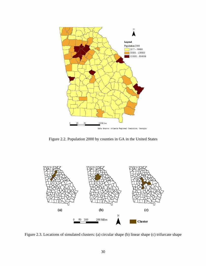
30

Figure 2.2. Population 2000 by counties in GA in the United States

Figure 2.3. Locations of simulated clusters: (a) circular shape (b) linear shape (c) trifurcate shape

31

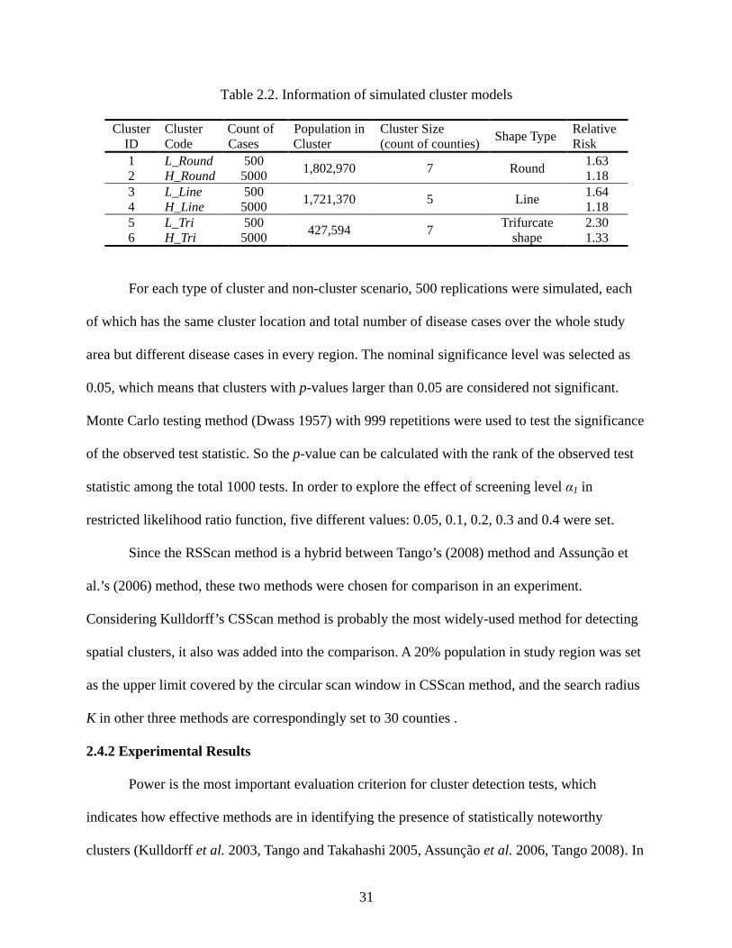
Table 2.2. Information of simulated cluster models

Cluster ID

Cluster Code

Count of Cases

Population in Cluster

Cluster Size (count of counties) Shape Type Relative

Risk 1 L_Round 500 1,802,970 7 Round 1.63 2 H_Round 5000 1.18 3 L_Line 500 1,721,370 5 Line 1.64 4 H_Line 5000 1.18 5 L_Tri 500 427,594 7 Trifurcate

shape 2.30

6 H_Tri 5000 1.33

For each type of cluster and non-cluster scenario, 500 replications were simulated, each

of which has the same cluster location and total number of disease cases over the whole study

area but different disease cases in every region. The nominal significance level was selected as

0.05, which means that clusters with p-values larger than 0.05 are considered not significant.

Monte Carlo testing method (Dwass 1957) with 999 repetitions were used to test the significance

of the observed test statistic. So the p-value can be calculated with the rank of the observed test

statistic among the total 1000 tests. In order to explore the effect of screening level α1 in

restricted likelihood ratio function, five different values: 0.05, 0.1, 0.2, 0.3 and 0.4 were set.

Since the RSScan method is a hybrid between Tango’s (2008) method and Assunção et

al.’s (2006) method, these two methods were chosen for comparison in an experiment.

Considering Kulldorff’s CSScan method is probably the most widely-used method for detecting

spatial clusters, it also was added into the comparison. A 20% population in study region was set

as the upper limit covered by the circular scan window in CSScan method, and the search radius

K in other three methods are correspondingly set to 30 counties .

2.4.2 Experimental Results

Power is the most important evaluation criterion for cluster detection tests, which

indicates how effective methods are in identifying the presence of statistically noteworthy

clusters (Kulldorff et al. 2003, Tango and Takahashi 2005, Assunção et al. 2006, Tango 2008). In

32

order to understand how well these methods identify the correct boundaries of a cluster, Kappa

Index of Agreement (KIA, De Smith et al. 2007) is chosen as a complimentary metric to the

power in this study since it not only shows the match degree between the detected cluster

estimates and the true clusters, but also excludes the probability that the cluster regions are

detected by chance. In this case, the KIA decreases the impacts on the evaluation caused by

different cluster model properties, such as study region size and cluster size. In order to easily

compare the performances of different methods or different screening level values in RSScan and

Tango’s method, the results of six cluster models were averaged in terms of the levels of disease

cases and shapes of clusters.

2.4.2.1 Estimated Power of Methods

The power in this study is defined as the ratio of statistically significant clusters detected

(significance level=0.05) to the count of replications for each cluster model (500). The results of

the power analysis for four spatial scan methods are shown in Table 2.3. The highest value for

each scenario (column in the table) is bold. The test statistics in Assunção et al.’s method and

CSScan method can be regarded as the restricted likelihood ratio with α1=1.

We can see that all four methods have higher power to detect significant clusters with

lower level of disease cases (L_Cas) than those with higher level of disease cases (H_Cas). With

the increase of α1 from 0.05 to 0.4, RSScan method is easier to detect the significant clusters in

the shapes varying from linear shape (Line) to round shape (Round) and then to trifurcate shape

(Tri), while Tango’s method is easier to detect the significant clusters in the shapes varying from

linear shape (Line) to round shape (Round) but more difficult for the trifurcate shaped clusters

(Tri) whatever the value of α1 is. Assunção et al.’s method and CSScan method both have highest

powers for trifurcate shaped clusters (Tri). However, Assunção et al.’s method is more difficult to

33

detetct significnat round clusters (Round) while CSScan method has the lowest power for linear

clusters (Line).

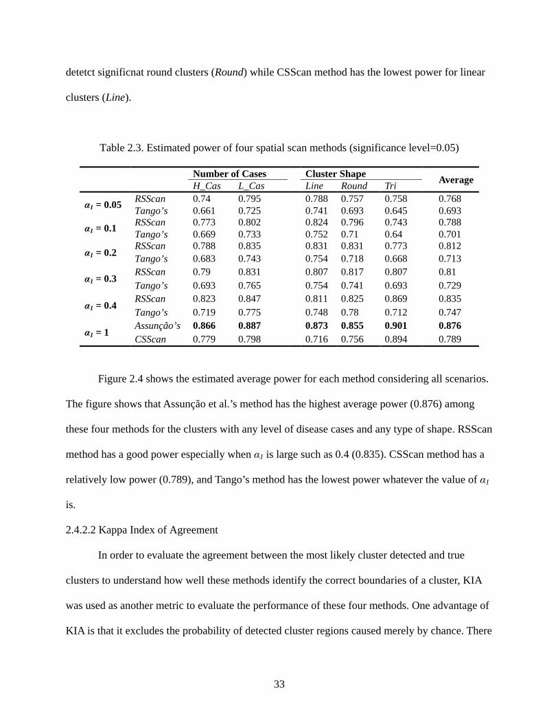
Table 2.3. Estimated power of four spatial scan methods (significance level=0.05)

Number of Cases Cluster Shape Average H_Cas L_Cas Line Round Tri

α1 = 0.05 RSScan 0.74 0.795 0.788 0.757 0.758 0.768 Tango’s 0.661 0.725 0.741 0.693 0.645 0.693

α1 = 0.1 RSScan 0.773 0.802 0.824 0.796 0.743 0.788 Tango’s 0.669 0.733 0.752 0.71 0.64 0.701

α1 = 0.2 RSScan 0.788 0.835 0.831 0.831 0.773 0.812 Tango’s 0.683 0.743 0.754 0.718 0.668 0.713

α1 = 0.3 RSScan 0.79 0.831 0.807 0.817 0.807 0.81 Tango’s 0.693 0.765 0.754 0.741 0.693 0.729

α1 = 0.4 RSScan 0.823 0.847 0.811 0.825 0.869 0.835 Tango’s 0.719 0.775 0.748 0.78 0.712 0.747

α1 = 1 Assunção’s 0.866 0.887 0.873 0.855 0.901 0.876 CSScan 0.779 0.798 0.716 0.756 0.894 0.789

Figure 2.4 shows the estimated average power for each method considering all scenarios.

The figure shows that Assunção et al.’s method has the highest average power (0.876) among

these four methods for the clusters with any level of disease cases and any type of shape. RSScan

method has a good power especially when α1 is large such as 0.4 (0.835). CSScan method has a

relatively low power (0.789), and Tango’s method has the lowest power whatever the value of α1

is.

2.4.2.2 Kappa Index of Agreement

In order to evaluate the agreement between the most likely cluster detected and true

clusters to understand how well these methods identify the correct boundaries of a cluster, KIA

was used as another metric to evaluate the performance of these four methods. One advantage of

KIA is that it excludes the probability of detected cluster regions caused merely by chance. There

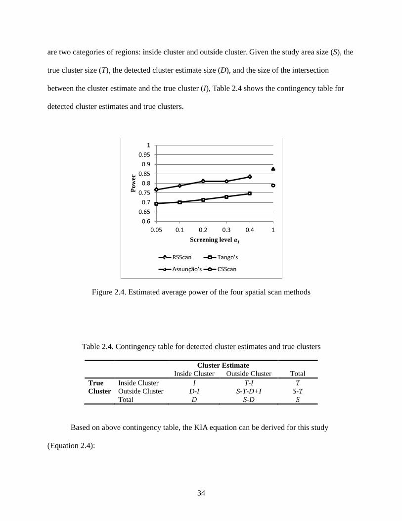
34

are two categories of regions: inside cluster and outside cluster. Given the study area size (S), the

true cluster size (T), the detected cluster estimate size (D), and the size of the intersection

between the cluster estimate and the true cluster (I), Table 2.4 shows the contingency table for

detected cluster estimates and true clusters.

Figure 2.4. Estimated average power of the four spatial scan methods

Table 2.4. Contingency table for detected cluster estimates and true clusters

Cluster Estimate Inside Cluster Outside Cluster Total True Cluster

Inside Cluster I T-I T Outside Cluster D-I S-T-D+I S-T

Total D S-D S

Based on above contingency table, the KIA equation can be derived for this study

(Equation 2.4):

0.6 0.65

0.7 0.75

0.8 0.85

0.9 0.95

1

0.05 0.1 0.2 0.3 0.4 1

Pow

er

Screening level α1

RSScan Tango's

Assunção's CSScan

35

EEO

−−

=1

κ Equation 2.4

( )S

IDTSIO +−−+= , ( ) ( )

2STSDSTDE −×−+×

=

where O is the observed proportion of matching values (the contingency table diagonal) and E is

the expected proportion of matches in this diagonal assuming the two categories in true cluster

are independent from the two categories in cluster estimate. KIA ranges from 0 to 1, and 1 means

a perfect agreement.

With the highest KIA value for each scenario (column in the table) in bold, Table 2.5

indicates that all methods have higher or close performance to identify the correct boundaries of

a cluster when there is a relatively low level of disease cases in the study region (L_Cas). With

the increase of α1 from 0.05 to 0.4, both RSScan and Tango’s methods are good at identifying the

boundaries of the clusters in the shapes varying from line (Line) to round (Round). The

boundaries of trifurcate shaped clusters (Tri) are difficult to be correctly identified by both

methods. Assunção et al.’s method is relatively better for clusters with trifurcate shape (Tri) than

other shapes, and CSScan method is good for round cluster (Round).

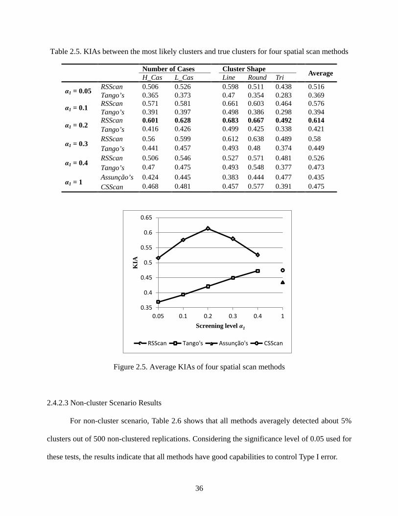
Figure 2.5 shows the average KIA value for each method considering all scenarios. The

figure indicates that RSScan method has a better performance to detect the boundaries of clusters

in various shapes than other three methods and peaks when α1 is 0.2 (0.614). The performance of

Tango’s method peaks when α1 is 0.4 and has a similar KIA value with CSScan method (about

0.47). Assunção et al.’s method has a relatively low power (0.435) possibly due to many low-risk

regions being involved into the cluster estimates.

36

Table 2.5. KIAs between the most likely clusters and true clusters for four spatial scan methods

Number of Cases Cluster Shape Average H_Cas L_Cas Line Round Tri

α1 = 0.05 RSScan 0.506 0.526 0.598 0.511 0.438 0.516 Tango’s 0.365 0.373 0.47 0.354 0.283 0.369

α1 = 0.1 RSScan 0.571 0.581 0.661 0.603 0.464 0.576 Tango’s 0.391 0.397 0.498 0.386 0.298 0.394

α1 = 0.2 RSScan 0.601 0.628 0.683 0.667 0.492 0.614 Tango’s 0.416 0.426 0.499 0.425 0.338 0.421

α1 = 0.3 RSScan 0.56 0.599 0.612 0.638 0.489 0.58 Tango’s 0.441 0.457 0.493 0.48 0.374 0.449

α1 = 0.4 RSScan 0.506 0.546 0.527 0.571 0.481 0.526 Tango’s 0.47 0.475 0.493 0.548 0.377 0.473

α1 = 1 Assunção’s 0.424 0.445 0.383 0.444 0.477 0.435 CSScan 0.468 0.481 0.457 0.577 0.391 0.475

Figure 2.5. Average KIAs of four spatial scan methods

2.4.2.3 Non-cluster Scenario Results

For non-cluster scenario, Table 2.6 shows that all methods averagely detected about 5%

clusters out of 500 non-clustered replications. Considering the significance level of 0.05 used for

these tests, the results indicate that all methods have good capabilities to control Type I error.

0.35

0.4

0.45

0.5

0.55

0.6

0.65

0.05 0.1 0.2 0.3 0.4 1

KIA

Screening level α1

RSScan Tango's Assunção's CSScan

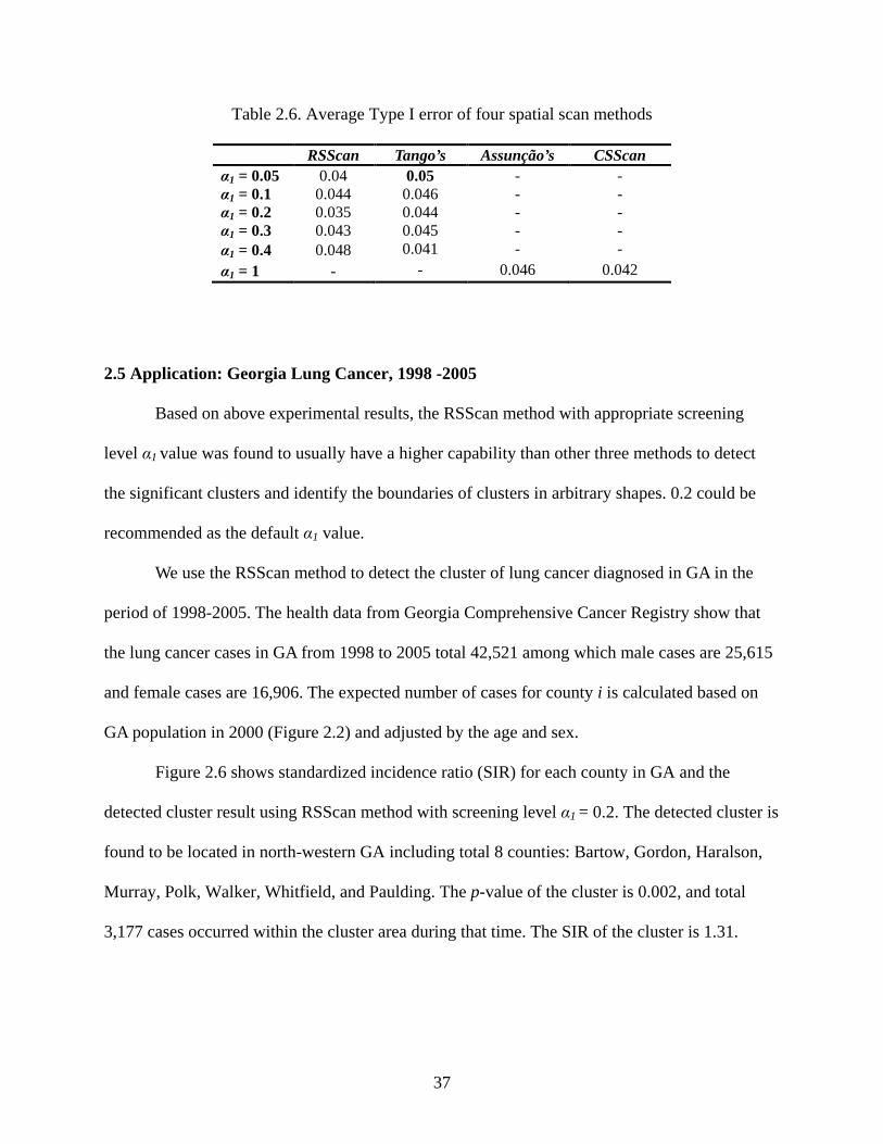
37

Table 2.6. Average Type I error of four spatial scan methods

RSScan Tango’s Assunção’s CSScan α1 = 0.05 0.04 0.05 - - α1 = 0.1 0.044 0.046 - - α1 = 0.2 0.035 0.044 - - α1 = 0.3 0.043 0.045 - - α1 = 0.4 0.048 0.041 - - α1 = 1 - - 0.046 0.042

2.5 Application: Georgia Lung Cancer, 1998 -2005

Based on above experimental results, the RSScan method with appropriate screening

level α1 value was found to usually have a higher capability than other three methods to detect

the significant clusters and identify the boundaries of clusters in arbitrary shapes. 0.2 could be

recommended as the default α1 value.

We use the RSScan method to detect the cluster of lung cancer diagnosed in GA in the

period of 1998-2005. The health data from Georgia Comprehensive Cancer Registry show that

the lung cancer cases in GA from 1998 to 2005 total 42,521 among which male cases are 25,615

and female cases are 16,906. The expected number of cases for county i is calculated based on

GA population in 2000 (Figure 2.2) and adjusted by the age and sex.

Figure 2.6 shows standardized incidence ratio (SIR) for each county in GA and the

detected cluster result using RSScan method with screening level α1 = 0.2. The detected cluster is

found to be located in north-western GA including total 8 counties: Bartow, Gordon, Haralson,

Murray, Polk, Walker, Whitfield, and Paulding. The p-value of the cluster is 0.002, and total

3,177 cases occurred within the cluster area during that time. The SIR of the cluster is 1.31.

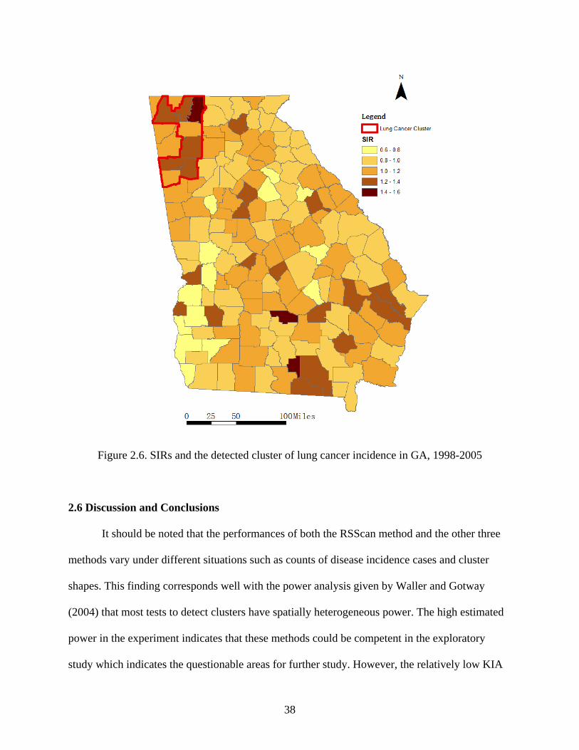
38

Figure 2.6. SIRs and the detected cluster of lung cancer incidence in GA, 1998-2005

2.6 Discussion and Conclusions

It should be noted that the performances of both the RSScan method and the other three

methods vary under different situations such as counts of disease incidence cases and cluster

shapes. This finding corresponds well with the power analysis given by Waller and Gotway

(2004) that most tests to detect clusters have spatially heterogeneous power. The high estimated

power in the experiment indicates that these methods could be competent in the exploratory

study which indicates the questionable areas for further study. However, the relatively low KIA

39

values indicate that these methods may be inappropriate for the applications which require

accurate boundaries of clusters, such as the analysis of the change of spatial clusters over time. In

order to get deeper insights about the spatio-temporal disease risk pattern, disease risk modeling,

such as spatio-temporal multilevel models, may be a better way.

Tango’s restricted likelihood ratio has good interpretability and strong power in detecting

disease clusters with circular scan window (Tango 2008). To our knowledge, however, there is no

previous work discussing its performance in detecting clusters in arbitrary shapes with other

search strategies. For the first time, this study implements and tests restricted likelihood ratio

combined with Assunção et al.’s dMST search strategy to quickly detect disease clusters in

arbitrary shapes. In order to understand the performance of this redesigned hybrid method in

various situations, more cluster models than Tango (2008) and Assunção et al. (2006) were

designed in this performance test, which includes six cluster models and two non-cluster

scenarios. These cluster models consider different numbers of disease cases in a study area and

various shapes of clusters. The choice of the screening level α1 in restricted likelihood ratio is

also explored when combined with Assunção et al.’s dMST search strategy in the RSScan

method. Besides the metric of power, this study proposes using KIA to evaluate and compare the

performances of cluster detection methods to identify the boundaries of clusters in order to avoid

the effects due to the different cluster model properties. Finally, the application of the RSScan

method was applied in a case of detecting the cluster of lung cancer in Georgia between 1998

and 2005.

The experimental results indicate that the RSScan method with appropriate screening

level α1 generally has higher or similar capability to quickly detect statistically significant

disease clusters and identify the boundaries of clusters than Tango’s method, Assunção et al.’s

40

method, and Kulldorff’s CSScan method under the same situation, especially for the clusters in

irregular shapes. Based on results of this study, 0.2 is recommended as a default for the screening

level α1 in the RSScan method.

41

References

Anselin, L., 1995. Local indicators of spatial association-lisa. Geographical analysis, 27 (2), 93-115.

Assunção, R., Costa, M., Tavares, A. & Ferreira, S., 2006. Fast detection of arbitrarily shaped disease clusters. Statistics in Medicine, 25 (5), 723-742.

Besag, J. & Newell, J., 1991. The detection of clusters in rare diseases. Journal of the Royal Statistical Society. Series A (Statistics in Society), 154 (1), 143-155.

De Smith, M., Goodchild, M. & Longley, P., 2007. Geospatial analysis: A comprehensive guide to principles, techniques and software tools: Troubador Publishing.

Duczmal, L. & Assunção, R., 2004. A simulated annealing strategy for the detection of arbitrarily shaped spatial clusters. Computational Statistics & Data Analysis, 45 (2), 269-286.

Duczmal, L., Kulldorff, M. & Huang, L., 2006. Evaluation of spatial scan statistics for irregularly shaped clusters. Journal of Computational and Graphical Statistics, 15 (2), 428-442.

Dwass, M., 1957. Modified randomization tests for nonparametric hypotheses. Annals of Mathematical Statistics, 28 (1), 181-187.

Goovaerts, P., 2010. Geostatistical analysis of county level lung cancer mortality rates in the southeastern united states. Geographical analysis, 42 (1), 32-52.

Jacquez, G. & Greiling, D., 2003. Local clustering in breast, lung and colorectal cancer in long island, new york. International Journal of Health Geographics, 2 (1), 3.

Kulldorff, M., 1997. A spatial scan statistic. Communications in Statistics-Theory and Methods, 26 (6), 1481-1496.

Kulldorff, M., Huang, L., Pickle, L. & Duczmal, L., 2006. An elliptic spatial scan statistic. Statistics in Medicine, 25 (22), 3929-3943.

42

Kulldorff, M. & Information Management Services Inc., 2010. Satscantm v9.1: Software for the spatial and space-time scan statistics. http://www.satscan.org/

Kulldorff, M. & Nagarwalla, N., 1995. Spatial disease clusters - detection and inference. Statistics in Medicine, 14 (8), 799-810.

Kulldorff, M., Tango, T. & Park, P.J., 2003. Power comparisons for disease clustering tests. Computational Statistics & Data Analysis, 42 (4), 665-684.

Lawson, A., 2006. Statistical methods in spatial epidemiology, 2nd ed. Chichester, England ; Hoboken, NJ: Wiley.

Maheswaran, R. & Craglia, M., 2004. Gis in public health practice Boca Raton: CRC Press.

Openshaw, S., Charlton, M., Wymer, C. & Craft, A., 1987. A mark 1 geographical analysis machine for the automated analysis of point data sets. International Journal of Geographical Information Systems, 1 (4), 335 - 358.

Rogerson, P. & Yamada, I., 2009. Statistical detection and surveillance of geographic clusters Boca Raton: CRC Press.

Takahashi, K., Yokoyama, T. & Tango, T., 2010. Flexscan v3.1: Software for the flexible scan statistic. http://www.niph.go.jp/soshiki/gijutsu/download/flexscan/index.html

Tango, T., 2008. A spatial scan statistic with a restricted likelihood ratio. Japanese Journal of Biometrics, 29 (2), 75-95.

Tango, T. & Takahashi, K., 2005. A flexibly shaped spatial scan statistic for detecting clusters. International Journal of Health Geographics, 4, 11-15.

Turnbull, B.W., Iwano, E.J., Burnett, W.S., Howe, H.L. & Clark, L.C., 1990. Monitoring for clusters of disease - application to leukemia incidence in upstate new-york. American Journal of Epidemiology, 132 (1), S136-S143.

Waller, L. & Gotway, C., 2004. Applied spatial statistics for public health data: Wiley-Interscience.

http://www.satscan.org/�

http://www.niph.go.jp/soshiki/gijutsu/download/flexscan/index.html�

43

Yiannakoulias, N., Rosychuk, R.J. & Hodgson, J., 2007. Adaptations for finding irregularly shaped disease clusters. International Journal of Health Geographics, 6 (1), 28.

44

CHAPTER 3

HIERARCHICAL BAYESIAN MODELING OF THE SPATIO-TEMPORAL PATTERNS OF

LUNG CANCER INCIDENCE RISKS IN GEORGIA, 2000-20072

2 Yin, P., Mu, L., Madden, M. and Vena, J. To be submitted to International Journal of Health

Geographics.

45

Abstract

Lung cancer is the second most commonly diagnosed cancer in men and women in

Georgia. However, the related studies about the patterns of lung cancer in Georgia at a fine

spatio-temporal scale are very limited. In this study, hierarchical Bayesian models are used to

explore the spatio-temporal patterns of lung cancer incidence risks by race and sex in Georgia for

the period of 2000 to 2007. With the census tract level as the spatial scale and the two-year

period aggregation as the temporal scale, we propose and compare a total of seven Bayesian

spatio-temporal models including two under the separate modeling framework and five models

under the joint modeling framework. One of these models is finally chosen and its results clearly

show that the northwest region of Georgia has stably elevated lung cancer incidence risks for all

population groups during the study period. Showing more detailed and reliable variations of the

lung cancer incidence risks in space and time, our study aims to better support assessing

healthcare performance, establishing etiological hypotheses, and making effective and efficient

health policies. In addition, our study shows that there are strong inverse relationships between

the socioeconomic status (SES) and the lung cancer incidence risk in Georgia males, especially

white males, and weak inverse relationships in both white and black Georgia females. The study

results are expected to lead to further studies including, the spatial and temporal random effects

in the models that may provide some implications on the potential disease risk factors for further

ecological studies. The limitations of this study including the lack of smoking data and

population estimation error are also discussed in the end.

Keywords: Bayesian model, Spatio-temporal pattern, Lung cancer, Socioeconomic status,

Georgia

46

3.1 Introduction

Lung cancer is not only the second most commonly diagnosed cancer in men and women,

but also the leading cause of cancer-related death in Georgia in the United States (Georgia

Department of Public Health 2008). However, as far as we know, the lung cancer studies in

Georgia are very few, and most of these mainly focus on descriptive analyses using crude rates at

a coarse spatio-temporal scale, such as the 5-year incidence rates at the health district or county

level. Such analytical results usually obscure the detailed variations of lung cancer risks in space

and time, and could introduce inferential biases on etiological hypotheses. In addition, they can

only provide limited help for healthcare performance assessment and health policy making to

improve the efficiency of interventions and the distribution of resources.

The small number problem is one of the challenges for mapping lung cancer risk at a fine

spatio-temporal scale. For rare diseases such as cancers, the total counts of cases could become

very sparse at some fine spatio-temporal scales, especially when more demographic dimensions

are also considered, such as sex, age, race, among others. With the sparseness of the counts,

some traditional estimates of disease risk or relative risk, such as the Standardized Incidence

Ratio (SIR), could become unreliable and may lead to a large misunderstanding of the true

disease risk due to high sampling variability. Recently, hierarchical Bayesian models have been

widely used to map disease risk spatially or spatio-temporally (Bernardinelli et al. 1995, Waller

et al. 1997, Xia and Carlin 1998, Knorr-Held 2000, Mollié 2001, Wakefield et al. 2001, Best et

al. 2005, Richardson et al. 2006, Abellan et al. 2008, Lawson 2009, Fortunato et al. 2011). For

sparse count data, integrating both data fit and subjective prior information makes Bayesian

models possible to mitigate the inferential biases of frequentist methods that totally depend on

data fit. In addition, it is easy to develop model-based spatial and spatio-temporal smoothing

47

methods under the Bayesian framework that not only consider the effects of disease risk factors,

but also borrow strengths from neighboring areas and/or time periods.

In this study, we use hierarchical Bayesian models to explore the spatial-temporal

patterns of lung cancer incidence risks in Georgia. The analyses are conducted for four

population groups stratified by sex and race at the census tract level over four two-year periods

from 2000-2007. A total of seven spatio-temporal models under two modeling frameworks were

proposed and compared. One framework is to model the relative risks (RRs) of each population

group separately, and the other framework is to jointly model the RRs of each population group

under the assumption that some common disease risk factors exist in all population groups. One

model is finally chosen based on some criterion and its results are interpreted. The aim of the

study is to obtain reliable spatio-temporal patterns of lung cancer incidence risks by sex and race

in Georgia at a fine scale, which are expected to identify the spatio-temporal hot-spots of the

disease risks of a specific population group for further study, and help to facilitate the related

health policy making in Georgia. In addition, evaluating the effects of area-based socioeconomic

status (SES) on the lung cancer incidence risks in each population group is also explored in the

modeling. The understandings of the socioeconomic gradients in lung cancer incidence risks by

race and sex could provide some implications on how to reduce the lung cancer disparities in

Georgia. This paper will be organized as follows. In the next section, the study area and data

sources are described. Then, the method for population estimation, the area-based SES measure,

and the seven Bayesian spatio-temporal models under the two modeling frameworks are

explained. Next, the modeling results and discussions are given, followed by some conclusions.

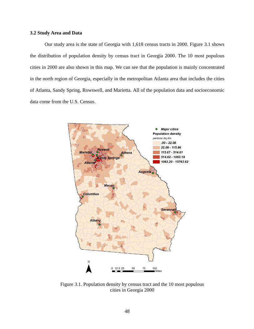
48

3.2 Study Area and Data

Our study area is the state of Georgia with 1,618 census tracts in 2000. Figure 3.1 shows

the distribution of population density by census tract in Georgia 2000. The 10 most populous

cities in 2000 are also shown in this map. We can see that the population is mainly concentrated

in the north region of Georgia, especially in the metropolitan Atlanta area that includes the cities

of Atlanta, Sandy Spring, Rowswell, and Marietta. All of the population data and socioeconomic

data come from the U.S. Census.

Figure 3.1. Population density by census tract and the 10 most populous cities in Georgia 2000

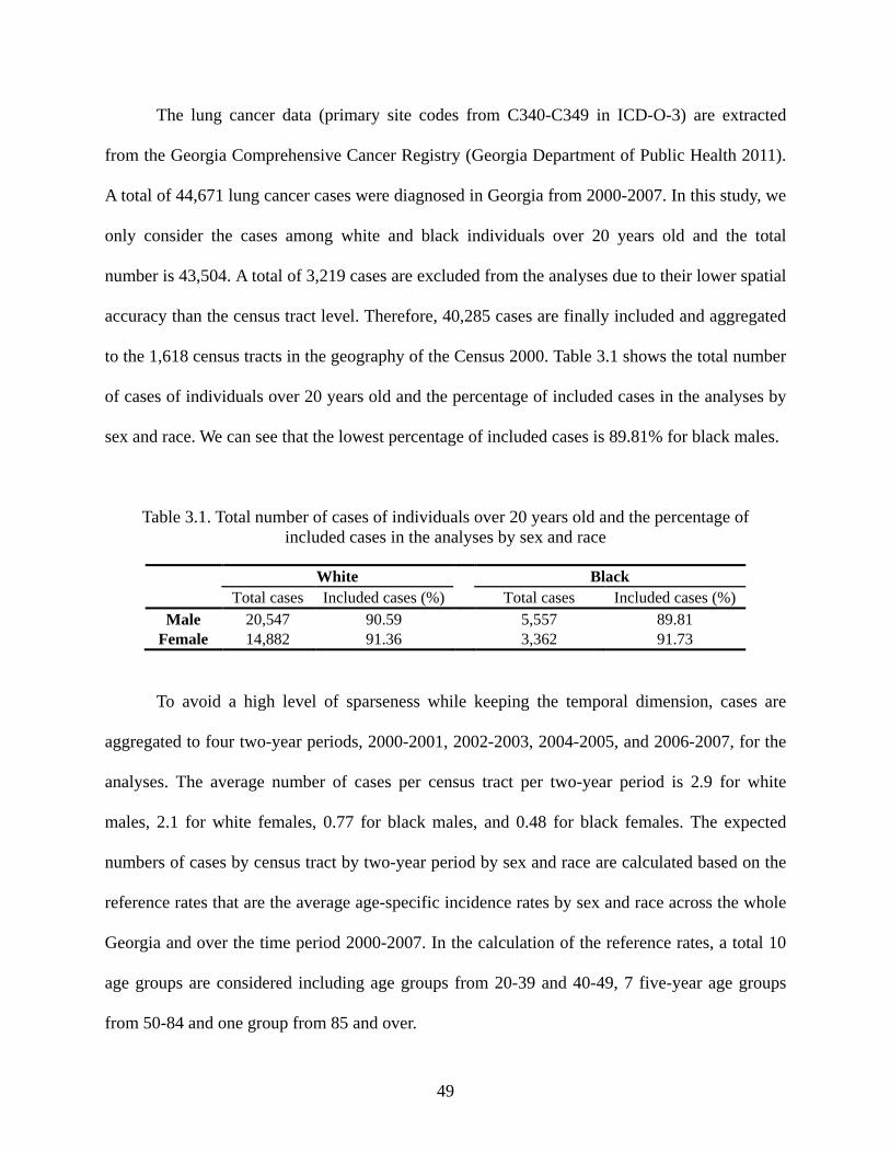
49

The lung cancer data (primary site codes from C340-C349 in ICD-O-3) are extracted

from the Georgia Comprehensive Cancer Registry (Georgia Department of Public Health 2011).

A total of 44,671 lung cancer cases were diagnosed in Georgia from 2000-2007. In this study, we

only consider the cases among white and black individuals over 20 years old and the total

number is 43,504. A total of 3,219 cases are excluded from the analyses due to their lower spatial

accuracy than the census tract level. Therefore, 40,285 cases are finally included and aggregated

to the 1,618 census tracts in the geography of the Census 2000. Table 3.1 shows the total number

of cases of individuals over 20 years old and the percentage of included cases in the analyses by

sex and race. We can see that the lowest percentage of included cases is 89.81% for black males.

Table 3.1. Total number of cases of individuals over 20 years old and the percentage of included cases in the analyses by sex and race

White Black Total cases Included cases (%) Total cases Included cases (%)

Male 20,547 90.59 5,557 89.81 Female 14,882 91.36 3,362 91.73

To avoid a high level of sparseness while keeping the temporal dimension, cases are

aggregated to four two-year periods, 2000-2001, 2002-2003, 2004-2005, and 2006-2007, for the

analyses. The average number of cases per census tract per two-year period is 2.9 for white

males, 2.1 for white females, 0.77 for black males, and 0.48 for black females. The expected

numbers of cases by census tract by two-year period by sex and race are calculated based on the

reference rates that are the average age-specific incidence rates by sex and race across the whole

Georgia and over the time period 2000-2007. In the calculation of the reference rates, a total 10

age groups are considered including age groups from 20-39 and 40-49, 7 five-year age groups

from 50-84 and one group from 85 and over.

50

3.3 Methods

3.3.1 Population Estimation for Intercensal Years

The population at risk is important to accurately calculate expected cases and estimate

disease risk. However, the census population data at the tract level are only available at the

census years (e.g. 2000 and 2010). It is also noted that the geographic boundaries of census tracts

vary every census year. For example, there are a total of 1,618 tracts in Census 2000, while a

total of 1,969 tracts exist in Census 2010. At the county level, the Census Bureau (Population

Estimates Program 2011) provides the estimates of population by race, sex and age for each

intercensal year. In this study, the boundaries of census tracts in 2000 are used as the standard

geography for the whole study period. With the census population data currently available, one

of the interpolation methods proposed by Best and Wakefield (1999) is used to estimate the

population by race, sex and age at the census tract level for each intercensal year.

The steps of the population estimation are as follows. First, we use the overlay function in

the Geographical Information System (GIS), ArcGISTM (ESRI, Inc.) and the areal weighting

interpolation method (Goodchild and Lam 1980) to estimate the population in 2010 using the

geography of the 2000 census tracts. To improve the accuracy, we use the 2010 population data

at the block level instead of the tract level since blocks are at a finer spatial scale. Then, for each

population group by race, sex and age in a county, we assume the population N are

multinomially distributed to the census tracts in that county with a vector of apportionment

probabilities p=(p1,…,pI)T, where I denotes the number of census tracts in that county and pi is

the proportion of the population in census tract i in the population of the county N. The

probabilities p for each intercensal year is estimated via a simple linear interpolation between the

censuses (i.e., 2000 and 2010).

51

Based on the population estimates, the reference rates for all population groups are then

calculated. Using the U.S. 2000 standard population for standardization, the direct age-adjusted

(over 20 years old) lung cancer incidence annual rates (per 100000 population) in Georgia (2000-

2007) are 132.7 for white males, 75.3 for white females, 135.2 for black males, and 54.5 for

black females.

3.3.2 Area-based SES Measure

Due to the relative homogeneity, the area-based SES measure at the census tract level

could be a good surrogate of individual SES in a health study when individual SES is unavailable

(Krieger 1992). Detailed discussions of area-based SES measures can be found in the literature

(Krieger et al. 1997, Carstairs 2001, Krieger et al. 2002, Darden et al. 2009). Various single

variable or composite measures can capture different aspects of socioeconomic characteristics. In

this study, we use the modified Darden-Kamel Composite Index (Darden et al. 2009) to measure

the SES at the census tract level, and evaluate its relationships with the lung cancer incidence

risks by race and sex. The modified Darden-Kamel Composite Index is an average Z score of

total nine socioeconomic variables in U.S. census data (Table 3.2).

Table 3.2. Variables incorporated in the modified Darden-Kamel Composite Index

Modified Darden-Kamel Composite Index 1. Percentage of residents with university degrees 2. Median household income 3. Percentage of managerial and professional positions 4. Median value of dwelling 5. Median gross rent of dwelling 6. Percentage of homeownership 7. Percentage below poverty 8. Unemployment rate 9. Percentage of households with vehicle

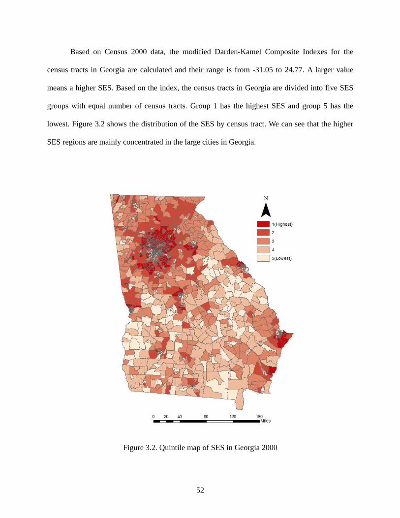
52

Based on Census 2000 data, the modified Darden-Kamel Composite Indexes for the

census tracts in Georgia are calculated and their range is from -31.05 to 24.77. A larger value

means a higher SES. Based on the index, the census tracts in Georgia are divided into five SES

groups with equal number of census tracts. Group 1 has the highest SES and group 5 has the

lowest. Figure 3.2 shows the distribution of the SES by census tract. We can see that the higher

SES regions are mainly concentrated in the large cities in Georgia.

Figure 3.2. Quintile map of SES in Georgia 2000

53

3.3.3 Bayesian Spatio-temporal Models

Bayesian models have naturally hierarchical structures. At the first level, the number of

observed cases yitk for census tract i =1,…,1618, time period t =1,…,4 and population group by

race and sex k =1,…,4 is assumed to follow a Poisson distribution with mean EitkRitk, where Eitk

and Ritk are respectively the known expected number of cases and the unknown RR compared to

the corresponding reference risk (measured by the reference rate of specific population group) in

census tract i, time period t and population group k. At the second level, the logarithms of RRs

are decomposed into fixed effects for those measured risk factors such as the SES, and random

effects for those unmeasured or unobserved risk factors. In Bayesian spatio-temporal models,

three random effects are usually considered: spatial random main effect, temporal random main

effect and spatio-temporal interaction random effect. Both spatial and temporal random main

effects could be further divided into a structured component and an unstructured component,

which reflect the dependent and heterogeneous variations of risks in space and time, respectively.

In the Bayesian paradigm, prior distributions are needed to be assigned to the model parameters

and the random effects. Then, the references are made based on the posterior distributions of the

parameters and random effects derived from simulations.

In this study, we model the RR of each population group individually under two

modeling frameworks. The first framework is separate modeling where each population group

has an independent set of random effects. The second framework is joint modeling where there

are shared random effects representing some common unmeasured or unknown risk factors

among all the population groups. This joint modeling framework has been used to map one

disease for multiple population groups or multiple diseases that have common risk factors

(Knorr-Held and Best 2001, Held et al. 2005, Richardson et al. 2006, Downing et al. 2008). We

54

compare a total of seven models including two separate models and five joint models. Table 3.3

shows the components of the logarithms of RRs in each model.

Table 3.3. Components of logarithms of RRs in the seven Bayesian spatio-temporal models

Model Type Model # Logarithms of RRs

Separate Model1 tkikkitkR ξλα +++= i

Tk xβlog )(

Model2 itktkikkitkR υξλα ++++= i

Tk xβlog )(

Joint

Model3 itktkikkitkR ωςδφδα ++++= ,2,1)( iTk xβlog

Model4 tkiktkikkitkR ξλςδφδα +++++= ,2,1)( iTk xβlog

Model5 tkikittkikkitkR ξλθςδφδα ++++++= ,2,1)( iTk xβlog

Model6 itktkiktkikkitkR ωξλςδφδα ++++++= ,2,1)( iTk xβlog

Model7 itktkikittkikkitkR ωξλθςδφδα +++++++= ,2,1)( iTk xβlog

In each model, αk is the overall log-RR for population group k across the whole study area

over the whole study period, and βk are the coefficients associated with the SES group vector xi

for population group k. The difference among the seven models is in the components of random

effects. Separate models 1 and 2 both have spatial random main effect λik for population group k

in census tract i and temporal random main effect ξtk for population group k in time period t.

Model 2 also considers the spatio-temporal interaction υitk in census tract i and time period t for

population group k. In addition to the population-group-specific random effects like those in

separate models 1 and 2, joint models 3-7 also consider shared random effects across the four

population groups by race and sex. In these shared components of the joint models, ϕi represents

the shared spatial component in census tract i, and ϛt represents the shared temporal component

in time period t. The coefficients δ1,k and δ2,k allow gradients of the shared spatial and temporal

components among all the population groups. In models 5 and 7, a shared spatio-temporal

interaction θit is also considered. With respect to the population-group-specific random effects,

55

model 3 only considers a spatio-temporal interaction random effect ωitk for population group k,

and models 4 and 5 only consider specific spatial and temporal random main effects λik and ξtk.

For the two components λik and ξtk in models 4-7, We set them equal to 0 in white male models

(k=1) so that these two components in other population group models (k=2, 3 and 4) actually are

the differentials of the spatial and temporal random main effects between that population group

and white males.

Some early experiments show that only considering structured components in spatial and

temporal random main effects have better modeling results than considering both structured and

unstructured components. Therefore, the widely used Gaussian intrinsic conditional

autoregression normal (CAR normal) prior proposed by Besag et al. (1991) are assigned to the

spatial random main effects λik and ϕi and the temporal random main effects ξtk and ϛt to represent

the dependent variations of RRs over space and time. For a spatial random effect in an area, CAR

normal specifies that its conditional distribution, given all other spatial effects, is a normal

distribution with mean equal to the average spatial effects of its neighboring areas and variance

inversely proportional to the number of these neighbors. In this study, the spatial neighbors are

defined if they share a border or a vertex. For a temporal random effect in a time period, CAR

normal smoothes it towards the temporal effects of its temporal neighbors (i.e. the previous and

the next time periods).

Due to the lack of strong prior knowledge, vague prior distributions are used for other

parameters in the models based on current literature. We assign a flat prior on the overall log-RR

terms, αk, and assign independent Normal (0, 105) prior distributions to fixed effects βk. The

logarithms of the scaling parameters δ1,k and δ2,k are assigned independent Normal (0, 5) prior

distributions (Downing et al. 2008). With respect to the spatio-temporal interaction random

56

effects, independent normal prior distributions with means equal to 0 and precisions τυk, k

=1,…,4, are assigned to υitk in model 2 for each population group, independent normal prior

distributions with means equal to 0 and precisions τθ are assigned to θit in models 5 and 7, and a

multivariate normal prior distribution with covariance matrix Σ is assigned to ωitk in models 3, 6

and 7 to allow correlations amongst the population groups (Richardson et al. 2006, Downing et

al. 2008). Following the previous studies (Kelsall and Wakefield 1999, Best et al. 2005,

Downing et al. 2008), independent conjugate hyperpriors Gamma (0.5, 0.0005) are assigned to

all of the precision parameters in the normal priors for shared components τϕ, τϛ, τθ and for

population-group-specific components τλk, τξk, τυk, k =1,…,4. The covariance matrix Σ in the

multivariate normal prior is assigned a Wishart (Q, 4) distribution, where Q is set to be a

diagonal matrix with 0.01s (Richardson et al. 2006).

All of the models are constructed and run using WinBUGS software (Lunn et al. 2000).

For each model, two independent chains are run. The first 50,000 iterations are discarded as

burn-in to make sure inferences can be made based on converged simulations of the models.

Then, 10,000 iterations are run and every 10th is kept for reference. Therefore, the modeling

results are based on thinned samples of 2,000. Brooks-Gelman-Rubin diagnostics (Brooks and

Gelman 1998) and visual checks are used to assess convergence.

Similar to the joint mapping of male and female lung cancer risks by Richardson et al

(2006), the scaling parameters δ2,k are difficult to converge during the data fitting of models. This

could be because only four time periods cannot provide enough information to differentiate the

shared and specific temporal patterns. So, we fixed δ2,k = 1 for all joint models.

We use the deviance information criterion (DIC) to compare the seven models and choose

the best one to interpret. The DIC was proposed by Spiegelhalter et al (2002) as the sum of D

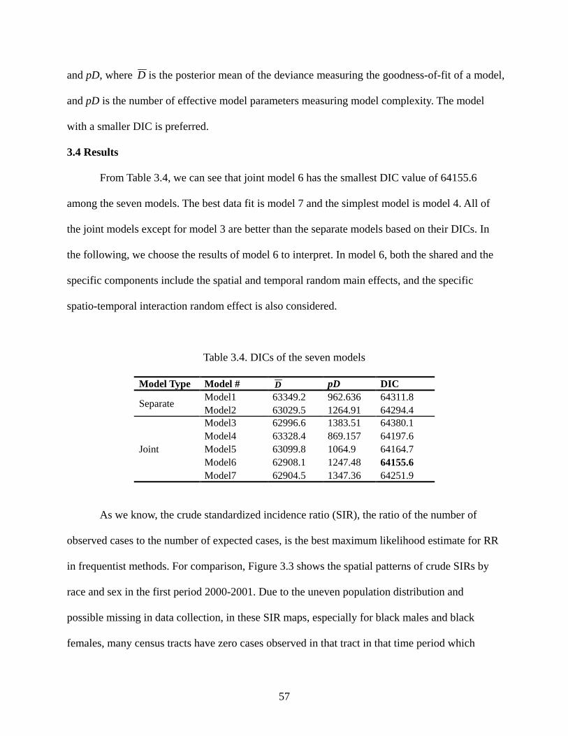
57

and pD, where D is the posterior mean of the deviance measuring the goodness-of-fit of a model,

and pD is the number of effective model parameters measuring model complexity. The model

with a smaller DIC is preferred.

3.4 Results

From Table 3.4, we can see that joint model 6 has the smallest DIC value of 64155.6

among the seven models. The best data fit is model 7 and the simplest model is model 4. All of

the joint models except for model 3 are better than the separate models based on their DICs. In

the following, we choose the results of model 6 to interpret. In model 6, both the shared and the

specific components include the spatial and temporal random main effects, and the specific

spatio-temporal interaction random effect is also considered.

Table 3.4. DICs of the seven models

Model Type Model # D pD DIC

Separate Model1 63349.2 962.636 64311.8 Model2 63029.5 1264.91 64294.4

Joint

Model3 62996.6 1383.51 64380.1 Model4 63328.4 869.157 64197.6 Model5 63099.8 1064.9 64164.7 Model6 62908.1 1247.48 64155.6 Model7 62904.5 1347.36 64251.9

As we know, the crude standardized incidence ratio (SIR), the ratio of the number of

observed cases to the number of expected cases, is the best maximum likelihood estimate for RR

in frequentist methods. For comparison, Figure 3.3 shows the spatial patterns of crude SIRs by

race and sex in the first period 2000-2001. Due to the uneven population distribution and

possible missing in data collection, in these SIR maps, especially for black males and black

females, many census tracts have zero cases observed in that tract in that time period which

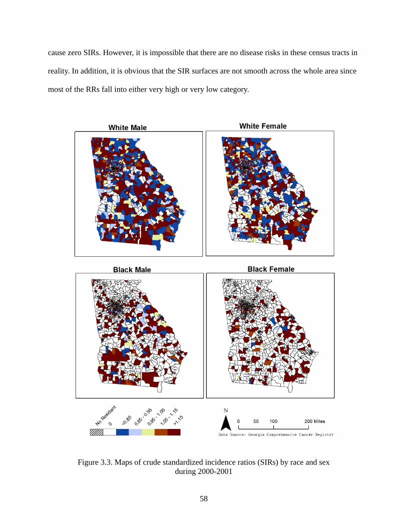
58

cause zero SIRs. However, it is impossible that there are no disease risks in these census tracts in

reality. In addition, it is obvious that the SIR surfaces are not smooth across the whole area since

most of the RRs fall into either very high or very low category.

Figure 3.3. Maps of crude standardized incidence ratios (SIRs) by race and sex during 2000-2001

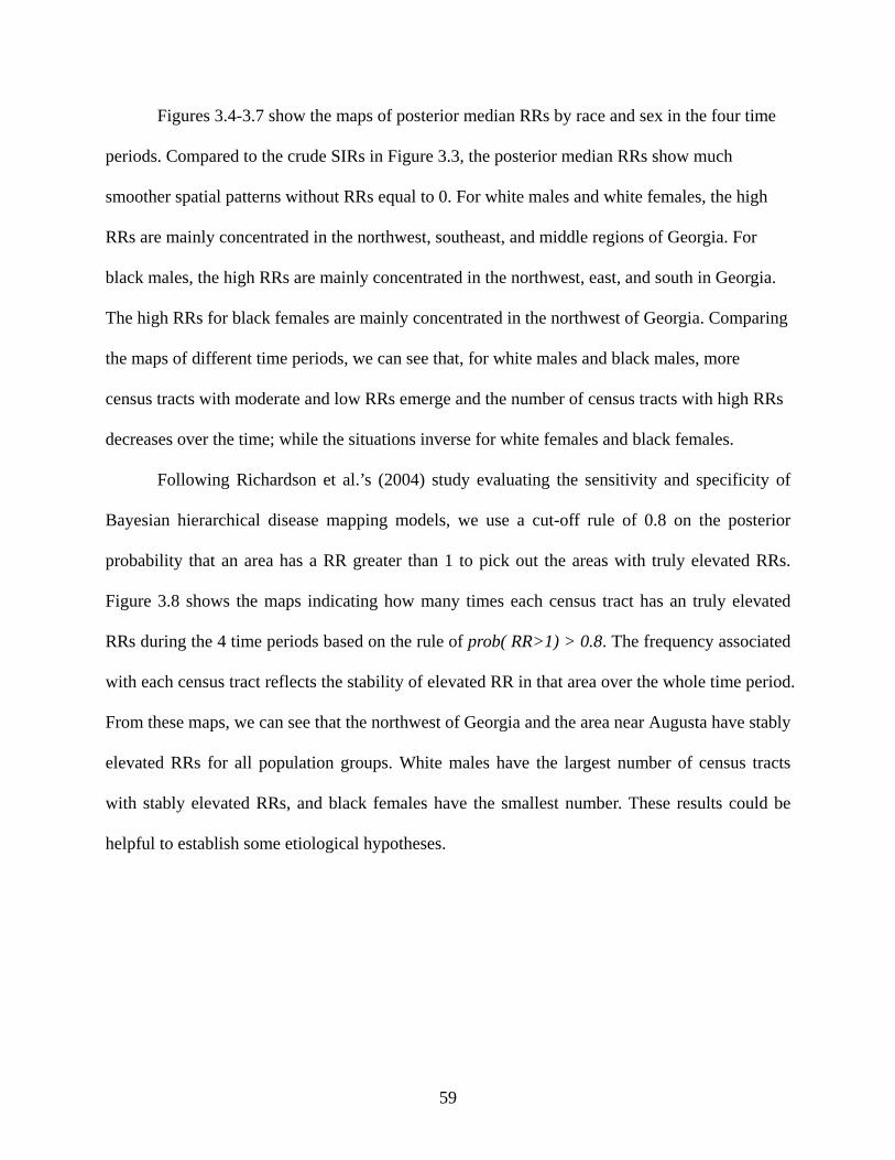
59

Figures 3.4-3.7 show the maps of posterior median RRs by race and sex in the four time

periods. Compared to the crude SIRs in Figure 3.3, the posterior median RRs show much

smoother spatial patterns without RRs equal to 0. For white males and white females, the high

RRs are mainly concentrated in the northwest, southeast, and middle regions of Georgia. For

black males, the high RRs are mainly concentrated in the northwest, east, and south in Georgia.

The high RRs for black females are mainly concentrated in the northwest of Georgia. Comparing

the maps of different time periods, we can see that, for white males and black males, more

census tracts with moderate and low RRs emerge and the number of census tracts with high RRs

decreases over the time; while the situations inverse for white females and black females.

Following Richardson et al.’s (2004) study evaluating the sensitivity and specificity of

Bayesian hierarchical disease mapping models, we use a cut-off rule of 0.8 on the posterior

probability that an area has a RR greater than 1 to pick out the areas with truly elevated RRs.

Figure 3.8 shows the maps indicating how many times each census tract has an truly elevated

RRs during the 4 time periods based on the rule of prob( RR>1) > 0.8. The frequency associated

with each census tract reflects the stability of elevated RR in that area over the whole time period.

From these maps, we can see that the northwest of Georgia and the area near Augusta have stably

elevated RRs for all population groups. White males have the largest number of census tracts

with stably elevated RRs, and black females have the smallest number. These results could be

helpful to establish some etiological hypotheses.

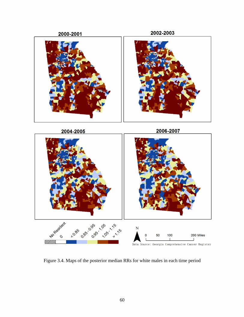
60

Figure 3.4. Maps of the posterior median RRs for white males in each time period

61

Figure 3.5. Maps of the posterior median RRs for white females in each time period

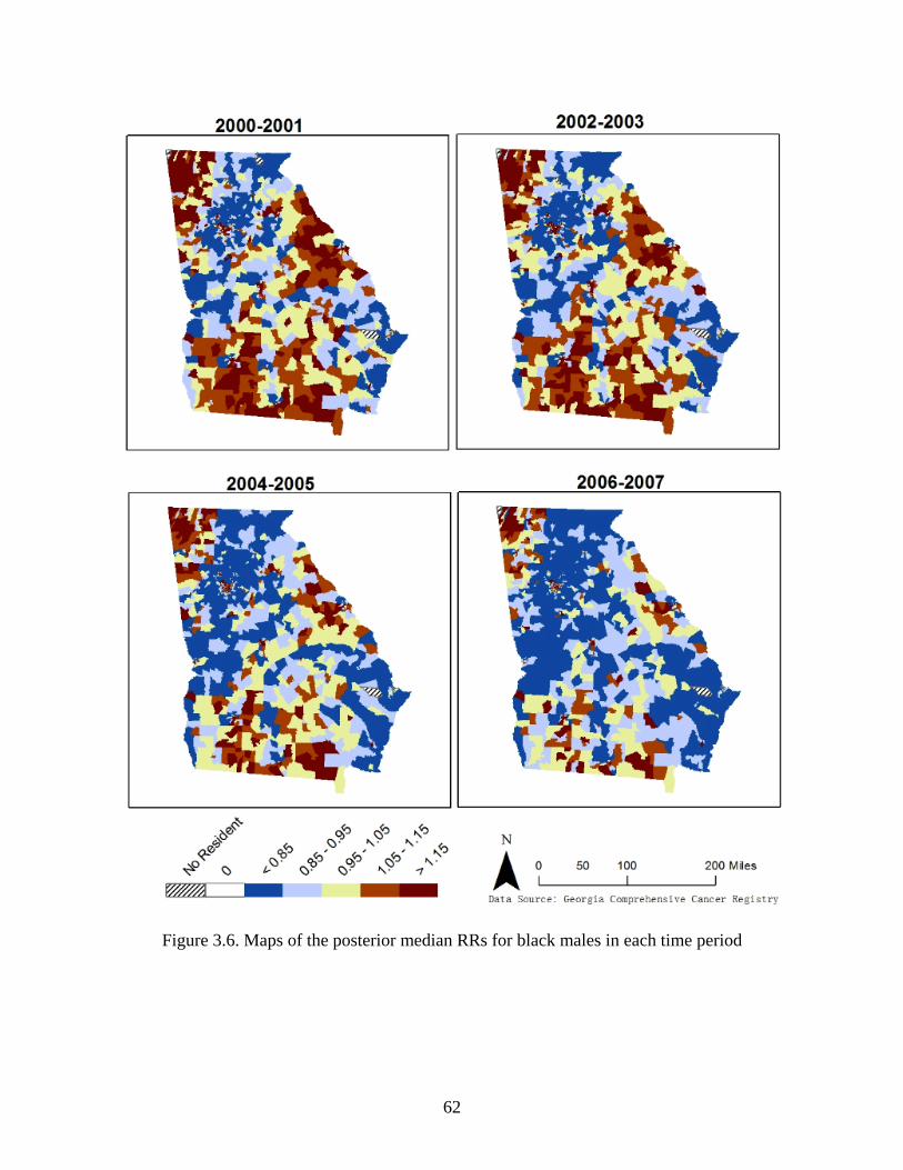
62

Figure 3.6. Maps of the posterior median RRs for black males in each time period

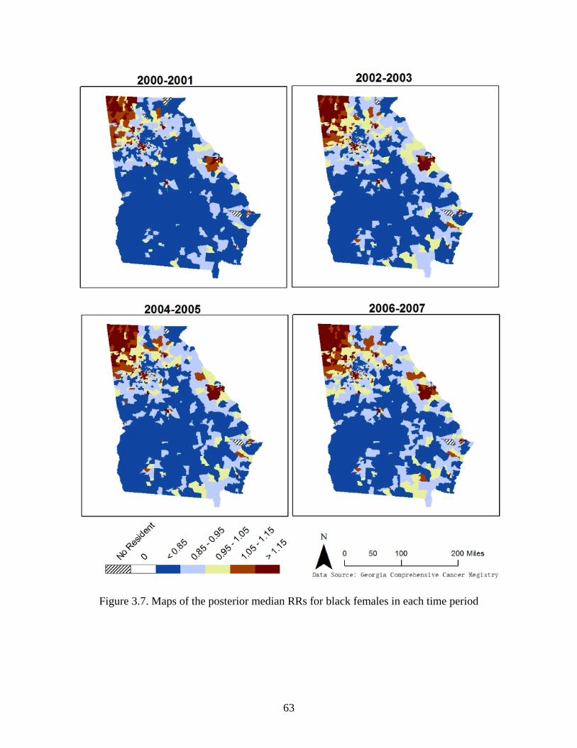
63

Figure 3.7. Maps of the posterior median RRs for black females in each time period

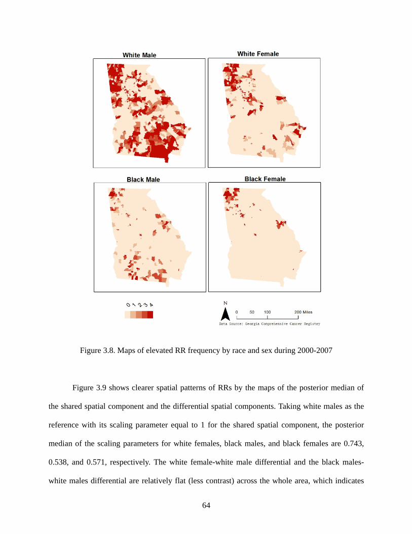
64

Figure 3.8. Maps of elevated RR frequency by race and sex during 2000-2007

Figure 3.9 shows clearer spatial patterns of RRs by the maps of the posterior median of

the shared spatial component and the differential spatial components. Taking white males as the

reference with its scaling parameter equal to 1 for the shared spatial component, the posterior

median of the scaling parameters for white females, black males, and black females are 0.743,

0.538, and 0.571, respectively. The white female-white male differential and the black males-

white males differential are relatively flat (less contrast) across the whole area, which indicates

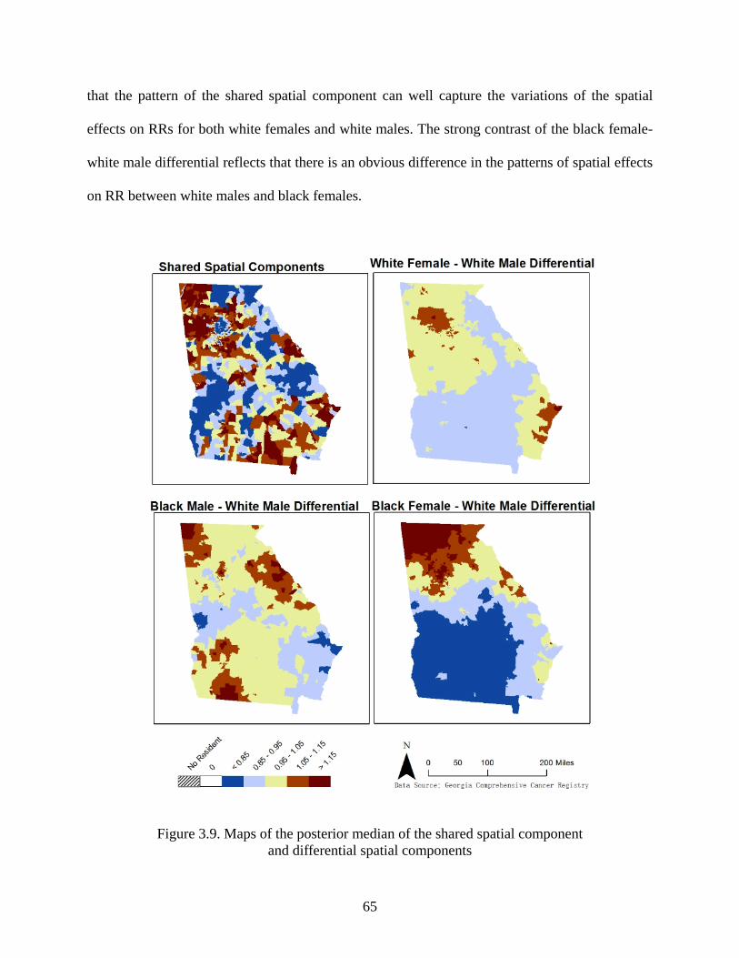
65

that the pattern of the shared spatial component can well capture the variations of the spatial

effects on RRs for both white females and white males. The strong contrast of the black female-

white male differential reflects that there is an obvious difference in the patterns of spatial effects

on RR between white males and black females.

Figure 3.9. Maps of the posterior median of the shared spatial component and differential spatial components

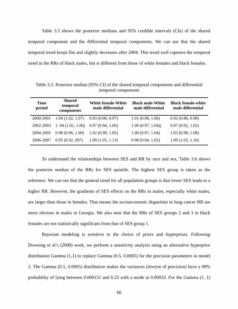
66

Table 3.5 shows the posterior medians and 95% credible intervals (CIs) of the shared

temporal component and the differential temporal components. We can see that the shared

temporal trend keeps flat and slightly decreases after 2004. This trend well captures the temporal

trend in the RRs of black males, but is different from those of white females and black females.

Table 3.5. Posterior median (95% CI) of the shared temporal components and differential temporal components

Time period

Shared temporal

components

White female-White male differential

Black male-White male differential

Black female-white male differential

2000-2001 1.04 (1.02, 1.07) 0.93 (0.90, 0.97) 1.01 (0.98, 1.06) 0.92 (0.86, 0.98)

2002-2003 1. 04 (1.01, 1.06) 0.97 (0.94, 1.00) 1.00 (0.97, 1.04)) 0.97 (0.92, 1.02)

2004-2005 0.98 (0.96, 1.00) 1.02 (0.99, 1.05) 1.00 (0.97, 1.04) 1.03 (0.98, 1.08)

2006-2007 0.95 (0.92, 097) 1.09 (1.05, 1.13) 0.98 (0.94, 1.02) 1.09 (1.03, 1.16)

To understand the relationships between SES and RR by race and sex, Table 3.6 shows

the posterior median of the RRs for SES quintile. The highest SES group is taken as the

reference. We can see that the general trend for all population groups is that lower SES leads to a

higher RR. However, the gradients of SES effects on the RRs in males, especially white males,

are larger than those in females. That means the socioeconomic disparities in lung cancer RR are

more obvious in males in Georgia. We also note that the RRs of SES groups 2 and 3 in black

females are not statistically significant from that of SES group 1.

Bayesian modeling is sensitive to the choice of priors and hyperpriors. Following

Downing et al’s (2008) work, we perform a sensitivity analysis using an alternative hyperprior

distribution Gamma (1,1) to replace Gamma (0.5, 0.0005) for the precision parameters in model

2. The Gamma (0.5, 0.0005) distribution makes the variances (inverse of precision) have a 99%

probability of lying between 0.000151 and 6.25 with a mode at 0.00033. For the Gamma (1, 1)

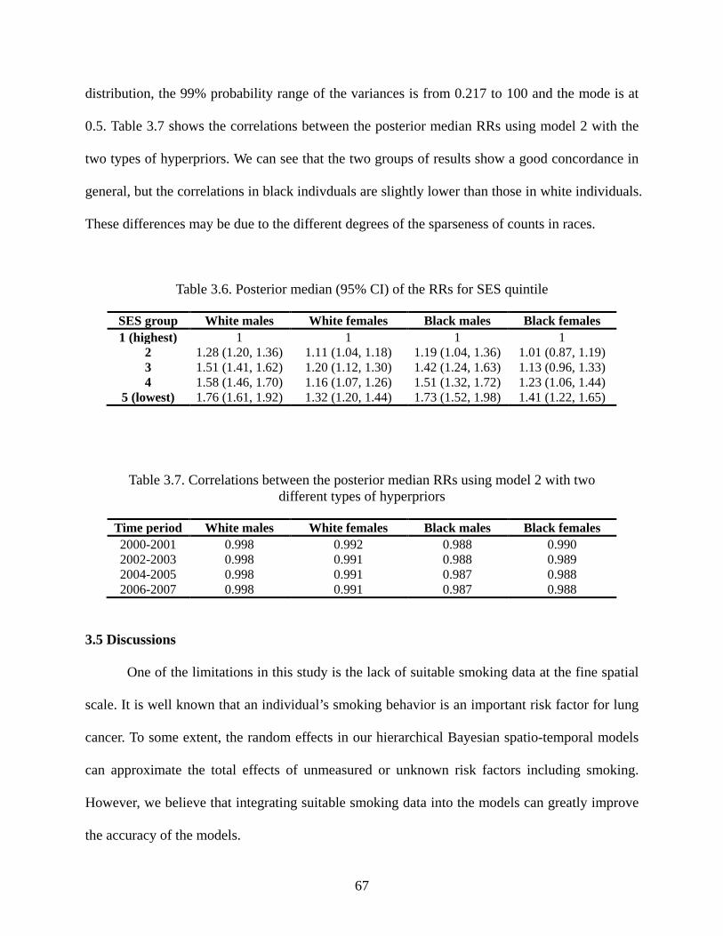
67

distribution, the 99% probability range of the variances is from 0.217 to 100 and the mode is at

0.5. Table 3.7 shows the correlations between the posterior median RRs using model 2 with the

two types of hyperpriors. We can see that the two groups of results show a good concordance in

general, but the correlations in black indivduals are slightly lower than those in white individuals.

These differences may be due to the different degrees of the sparseness of counts in races.

Table 3.6. Posterior median (95% CI) of the RRs for SES quintile

SES group White males White females Black males Black females 1 (highest) 1 1 1 1

2 1.28 (1.20, 1.36) 1.11 (1.04, 1.18) 1.19 (1.04, 1.36) 1.01 (0.87, 1.19) 3 1.51 (1.41, 1.62) 1.20 (1.12, 1.30) 1.42 (1.24, 1.63) 1.13 (0.96, 1.33) 4 1.58 (1.46, 1.70) 1.16 (1.07, 1.26) 1.51 (1.32, 1.72) 1.23 (1.06, 1.44)

5 (lowest) 1.76 (1.61, 1.92) 1.32 (1.20, 1.44) 1.73 (1.52, 1.98) 1.41 (1.22, 1.65)

Table 3.7. Correlations between the posterior median RRs using model 2 with two different types of hyperpriors

Time period White males White females Black males Black females 2000-2001 0.998 0.992 0.988 0.990 2002-2003 0.998 0.991 0.988 0.989 2004-2005 0.998 0.991 0.987 0.988 2006-2007 0.998 0.991 0.987 0.988

3.5 Discussions

One of the limitations in this study is the lack of suitable smoking data at the fine spatial

scale. It is well known that an individual’s smoking behavior is an important risk factor for lung

cancer. To some extent, the random effects in our hierarchical Bayesian spatio-temporal models

can approximate the total effects of unmeasured or unknown risk factors including smoking.

However, we believe that integrating suitable smoking data into the models can greatly improve

the accuracy of the models.

68

For the diseases with a long latency period such as cancers, lifetime exposures could be

important. In this study, we measure the area-based SES with Census 2000 data and assume they

could reflect the individual SES during the long latency period. This assumption could introduce

biases into the model inferences. In addition, the analysis of the relationship between disease RR

and SES is subject to the modifiable area unit problem (Openshaw and Taylor 1981). It means

that the references based on the analyses at current scale and/or unit definition may not be

generalized to other scales and/or unit definitions.

Estimation of population in small areas is a hot research topic in geography and statistics

recently. In our study, we use an apportionment method to estimate the population by race, sex

and age in each census tract in each intercensal year. Improvement of population estimation

model could greatly benefit the disease mapping models.

3.6 Conclusions

Facing the fact that there are a limited number of lung cancer studies in Georgia,

especially at a fine spatio-temporal scale, we use hierarchical Bayesian models to explore the

spatio-temporal patterns of lung cancer incidence risks in Georgia for the period 2000-2007. The

study is conducted at the census tract level using two-year time period as the temporal unit. The

fine spatial and temporal scales enable the study to show more detailed variations of lung cancer

incidence risks in space and time, which can better support healthcare performance assessment,

thereby establishing potential etiological hypotheses and making effective and efficient health

policies. Compared to the crude SIR, use of the Bayesian spatio-temporal model can provide a

more reliable estimate of disease risk in a fine spatio-temporal scale. The study also shows that

there are strong inverse relationships between SES and lung cancer incidence risk in males and

69

weak inverse relationships in females in Georgia. This could lead to further studies on the

underlying reasons such as occupational risk factors.

A total of seven Bayesian spatio-temporal models under the separate and joint modeling

frameworks are proposed and compared. In this study, the joint models generally have better

performance than the separate models using DIC as the criterion. Currently, our study is

primarily focusing on mapping the patterns of disease risks. However, the spatial and temporal

random effects in these disease mapping models may provide some implications on the potential

disease risk factors for further ecological studies.

70

References

Abellan, J.J., Richardson, S. & Best, N., 2008. Use of space–time models to investigate the stability of patterns of disease. Environmental health perspectives, 116 (8), 1111.

Bernardinelli, L., Clayton, D., Pascutto, C., Montomoli, C., Ghislandi, M. & Songini, M., 1995. Bayesian analysis of space—time variation in disease risk. Statistics in Medicine, 14 (21 22), 2433-2443.

Besag, J., York, J. & Mollié, A., 1991. Bayesian image restoration, with two applications in spatial statistics. Annals of the Institute of Statistical Mathematics, 43 (1), 1-20.

Best, N. & Jon, W., 1999. Accounting for inaccuracies in population counts and case registration in cancer mapping studies. Journal of the Royal Statistical Society. Series A (Statistics in Society), 162 (3), 363-382.

Best, N., Richardson, S. & Thomson, A., 2005. A comparison of bayesian spatial models for disease mapping. Statistical Methods in Medical Research, 14 (1), 35.

Brooks, S.P. & Gelman, A., 1998. Alternative methods for monitoring convergence of iterative simulations. Journal of Computational and Graphical Statistics, 7, 434-455.

Carstairs, V., 2001. 4.. Socio-economic factors at areal level and their relationship with health. Spatial Epidemiology, 1 (9), 51-68.

Darden, J., Rahbar, M., Jezierski, L., Li, M. & Velie, E., 2009. The measurement of neighborhood socioeconomic characteristics and black and white residential segregation in metropolitan detroit: Implications for the study of social disparities in health. Annals of the Association of American Geographers, 100 (1), 137-158.

Downing, A., Forman, D., Gilthorpe, M., Edwards, K. & Manda, S., 2008. Joint disease mapping using six cancers in the yorkshire region of england. International Journal of Health Geographics, 7 (1), 41.

Fortunato, L., Abellan, J.J., Beale, L., Lefevre, S. & Richardson, S., 2011. Spatio-temporal patterns of bladder cancer incidence in utah (1973-2004) and their association with the presence of toxic release inventory sites. International Journal of Health Geographics, 10 (1), 16.

71

Georgia Department of Public Health, 2008. Cancer program and data summary. Atlanta,GA.

Georgia Department of Public Health, 2011. Georgia comprehensive cancer registry [online]. http://www.health.state.ga.us/programs/gccr/ [Accessed Access Date 2011].

Goodchild, M.F. & Lam, N.S., 1980. Areal interpolation: A variant of the traditional spatial problem. Geo-Processing, 1, 297-312.

Held, L., Natário, I., Fenton, S.E., Rue, H. & Becker, N., 2005. Towards joint disease mapping. Statistical Methods in Medical Research, 14 (1), 61-82.

Kelsall, J. & Wakefield, J., 1999. Discussion of ' bayesian models for spatially correlated disease and exposure data', by best et al. In Bernardo, J., Berger, J., Dawid, A. & Smith, A. eds. Bayesian statistics 6. Oxford, UK: Oxford University Press, 151.

Knorr-Held, L., 2000. Bayesian modelling of inseparable space-time variation in disease risk. Statistics in Medicine, 19 (17-18), 2555-2567.

Knorr-Held, L. & Best, N.G., 2001. A shared component model for detecting joint and selective clustering of two diseases. Journal of the Royal Statistical Society: Series A (Statistics in Society), 164 (1), 73-85.

Krieger, N., 1992. Overcoming the absence of socioeconomic data in medical records: Validation and application of a census-based methodology. American Journal of Public Health, 82 (5), 703.

Krieger, N., Chen, J.T., Waterman, P.D., Soobader, M.J., Subramanian, S. & Carson, R., 2002. Geocoding and monitoring of us socioeconomic inequalities in mortality and cancer incidence: Does the choice of area-based measure and geographic level matter? American Journal of Epidemiology, 156 (5), 471.

Krieger, N., Williams, D.R. & Moss, N.E., 1997. Measuring social class in us public health research: Concepts, methodologies, and guidelines. Annual Review of Public Health, 18 (1), 341-378.

Lawson, A.B., 2009. Bayesian disease mapping: Hierarchical modeling in spatial epidemiology: Chapman & Hall/CRC.

http://www.health.state.ga.us/programs/gccr/�

72

Lunn, D.J., Thomas, A., Best, N. & Spiegelhalter, D., 2000. Winbugs-a bayesian modelling framework: Concepts, structure, and extensibility. Statistics and computing, 10 (4), 325-337.

Mollié, A., 2001. 15.. Bayesian mapping of hodgkins disease in france. Spatial Epidemiology, 1 (9), 267-286.

Openshaw, S. & Taylor, P.J., 1981. The modifiable areal unit problem. In Wrigley, N. & Bennett, R. eds. Quantitative geography: A british view. London and Boston: Routledge and Kegan Paul, 60-69.

Population Estimates Program, 2011. County intercensal estimates (2000-2010) [online]. http://www.census.gov/popest/data/intercensal/county/county2010.html [Accessed Access Date 2012].

Richardson, S., Abellan, J. & Best, N., 2006. Bayesian spatio-temporal analysis of joint patterns of male and female lung cancer risks in yorkshire (uk). Statistical Methods in Medical Research, 15 (4), 385.

Richardson, S., Thomson, A., Best, N. & Elliott, P., 2004. Interpreting posterior relative risk estimates in disease-mapping studies. Environmental health perspectives, 112 (9), 1016.

Spiegelhalter, D.J., Best, N.G., Carlin, B.P. & Van Der Linde, A., 2002. Bayesian measures of model complexity and fit. Journal of the Royal Statistical Society: Series B (Statistical Methodology), 64 (4), 583-639.

Wakefield, J., Best, N. & Waller, L., 2001. 7.. Bayesian approaches to disease mapping. Spatial Epidemiology, 1 (9), 104-128.

Waller, L., Carlin, B., Xia, H. & Gelfand, A., 1997. Hierarchical spatio-temporal mapping of disease rates. Journal of the American Statistical Association, 607-617.

Xia, H. & Carlin, B., 1998. Spatio-temporal models with errors in covariates: Mapping ohio lung cancer mortality. Statistics in Medicine, 17 (18), 2025-2043.

http://www.census.gov/popest/data/intercensal/county/county2010.html�

73

CHAPTER 4

MODULAR CAPACITATED MAXIMAL COVERING LOCATION PROBLEM FOR THE

OPTIMAL SITING OF EMERGENCY VEHICLES3

3 Yin, P. and Mu, L. 2012. Applied Geography 34: 247-254.

Reprinted here with permission of the publisher.

74

Abstract

To improve the application of the maximal covering location problem (MCLP), several

capacitated MCLP models were proposed to consider the capacity limits of facilities. However,

most of these models assume only one fixed capacity level for the facility at each potential site.

This assumption may limit the application of the capacitated MCLP. In this article, a modular

capacitated maximal covering location problem (MCMCLP) is proposed and formulated to allow

several possible capacity levels for the facility at each potential site. To optimally site emergency

vehicles, this new model also considers allocations of the demands beyond the service covering

standard. Two situations of the model are discussed: the MCMCLP-facility-constraint (FC),

which fixes the total number of facilities to be located, and the MCMCLP-non-facility-constraint

(NFC), which does not. In addition to the model formulations, one important aspect of location

modeling—spatial demand representation—is included in the analysis and discussion. As an

example, the MCMCLP is applied with Geographic Information System (GIS) and optimization

software packages to optimally site ambulances for the Emergency Medical Services (EMS)

Region 10 in the State of Georgia. The limitations of the model are also discussed.

Keywords: Modular capacitated MCLP, Spatial demand representation, GIS, Emergency vehicle

75

4.1 Introduction

Given a covering standard for a service, such as a distance or travel-time maximum, the

objective of the maximal covering location problem (MCLP) is to locate a fixed number of

facilities to provide the service to cover as many demands as possible. MCLP modeling, after

being put forward by Church and ReVelle (1974), has been a powerful and widely used tool in

many planning processes to optimally distribute limited resources to maximize social and

economic benefits, such as the placement of emergency warning sirens (Current and O'Kelly

1992), fire stations (Indriasari et al. 2010), distribution centers for humanitarian relief (Balcik

and Beamon 2008), health centers (Bennett et al. 1982, Verter and Lapierre 2002, Griffin et al.

2008, Ratick et al. 2009), and ecological reserves (Church et al. 1996). Among many different

versions of MCLP models that have been proposed, a basic underlying assumption is that the

facilities to be sited are uncapacitated. Under this assumption, the demand will be served as long

as it is within the service covering standard of any facility. However, this assumption of

uncapacitated facilities severely limits the application of covering models (Current and Storbeck

1988). Many service facilities have finite capacities to ensure an acceptable level of service and

spatial equity (Murray and Gerrard 1997, Liao and Guo 2008). For example, an ambulance base

can only respond to a limited number of demands within its service covering standard (e.g., 8-

min driving distance) at one time because of the availability status of the ambulances stationed at

the base. Therefore, the capacity limit—the main constraint addressed in this article—is an

important consideration in location problems, especially for the siting of emergency facilities.

Chung et al. (1983) and Current and Storbeck (1988) published two early papers dealing

with the capacitated versions of the MCLP. Both groups of authors added maximum capacity

constraints into the mathematical formulations of the MCLP to ensure that the demands allocated

76

to a facility will not exceed the capacity of that facility. However, these two capacitated MCLP

models only consider the allocation of the demands within the service covering standard of

facilities. Many systems, particularly public services, are typically available to all demands

within their jurisdiction. For example, even if a demand is located in an area where no

ambulances can reach the demand within a time standard, the demand must still be responded to

and be counted as part of some facility’s workload. Therefore, Pirkul and Schilling (1991)

proposed an extension of the capacitated MCLP where all demands are assigned to facilities,

regardless of whether that demand lies within the service covering standard. Such an idea of

allocating all demands to facilities is also shown in some uncapacitated MCLP models, such as

the generalized maximal covering location problem of Berman and Krass (2002). Following the

work of Pirkul and Schilling (1991), Haghani (1996) proposed a multi-objective capacitated

MCLP model where the objective function maximizes the weighted covered demand while

simultaneously minimizing the average distance from the uncovered demands to the located

facilities. He showed how to ensure the maximization of the weighted covered demand to be the

primary objective in the model by adjusting its weight in the objective function.

In all of the above capacitated MCLP models, only one fixed capacity level of the facility

is considered for each potential facility site. However, many situations arise where each potential

facility site could have several possible maximum capacity levels for a facility to choose. For

example, the capacity limit of an emergency facility (e.g., ambulance base or fire station) can be

assumed to be determined by its stationed emergency vehicles (e.g., ambulances or fire trucks).

Therefore, varied numbers of emergency vehicles will provide a series of possible maximum

capacity levels for the emergency facility to choose. Correia and Captivo (2003) called the

location problems with such capacity constraints modular capacitated location problems.

77

However, their model is an extension of the capacitated plant location problem, the objective of

which is to minimize total costs, including fixed costs and operating costs, associated with plant

and transportation costs, among others. For emergency services, the objective is often stated as

the minimization of losses to the public, which is equivalent to the maximization of benefits

(Indriasari et al. 2010). Cost is usually not the first consideration in these services. Therefore, the

capacitated MCLP is more suitable than the capacitated plant location problem for emergency

services. Although Griffin et al. (2008) considered three capability levels for each type of health

care facility in their capacitated MCLP model, there is no composing relationship for the

capacity levels of facilities, such as that between emergency vehicles and emergency facilities. In

addition, their model did not consider the allocation of demands outside the service covering

standard.

To apply the capacitated MCLP model to the emergency facility siting problem in which

an emergency facility could have different possible capacity levels with varied numbers of

stationed emergency vehicles, we propose an extension of the MCLP called the modular

capacitated maximal covering location problem (MCMCLP). Similar to the multi-objective

function in the model of Haghani (1996), the MCMCLP aims to maximize the weighted covered

demand while simultaneously minimizing the average distance from the uncovered demands to

the located facilities.

The remainder of this article is organized as follows: In the next section, the concepts,

formulations, and related issues of the MCMCLP are introduced and discussed in terms of two

situations. The first situation involves a fixed total number of facilities to be located; in the

second situation, the total number of facilities is not fixed. Subsequently, we briefly review the

approaches for spatial demand representation that could influence the accuracy of the problem

78

solutions. The method called service area spatial demand representation (SASDR) is briefly

described. Next, the MCMCLP and the SASDR are applied to the optimal siting of ambulances

for the Emergency Medical Services (EMS) Region 10 in the State of Georgia (GA). Finally, a

discussion and conclusions are provided.

4.2 Modular Capacitated Maximal Covering Location Problem (MCMCLP)

Because of the capacity limit of a facility, the allocation problem (i.e., how to allocate

demands to facilities) sometimes must be solved in conjunction with the location problem (i.e.,

where to site facilities) (Haghani 1996). Under the assumption that one demand can only be

allocated to, at most, one facility, we define three demand types and use them in the following

part of this article: 1) unallocated demand, which is not allocated to any facility (e.g., the

demands da and db in Figure 4.1); 2) covered allocated demand, which is located within the

service covering standard of a facility and is allocated to that facility (e.g., the demand dc in

Figure 4.1); 3) uncovered allocated demand, which is located beyond the service covering

standard of a facility but is allocated to that facility (e.g., the demand dd in Figure 4.1).

Figure 4.1. Illustration of three demand types: unallocated demand (da and db), covered allocated demand (dc), and uncovered allocated demand (dd)

da

db dc

dd

f

Facility

Demand

Allocated to

Service Covering

Standard

79

Following the work of Pirkul and Schilling (1991) and Haghani (1996), and in light of a

different perspective of the capacitated plant location problem of Correia and Captivo (2003), we

present an extension to the capacitated MCLP called MCMCLP and utilize it for siting

emergency services. In addition to the basic concept of the MCLP that the covered allocated

demands should be maximized by optimally siting a fixed number of facilities, the MCMCLP

also includes the following considerations: 1) the facility at each potential site has a maximum

capacity, which will be chosen from a finite and discrete set of available capacity levels; 2) all

demands need to be allocated to facilities (i.e., no unallocated demands exist), and the uncovered

allocated demands could be assigned on the basis of their proximity to facilities; 3) the demands

within a demand object, which is a spatial point or areal unit derived by abstracting or

partitioning continuous demand space, may be divided and allocated to multiple facilities.

An area with a larger population usually has a higher frequency of calls for emergency

service than an area with a smaller population. In addition, one emergency vehicle can only

respond to one call at a time and will be available only after that task is finished. Therefore, the

larger population an ambulance serves, the higher the busyness probability it usually has, the

longer the average response time for a call is, and the poorer the service it will provide. To

ensure an acceptable average response time for a call, each emergency vehicle can be thought to

have a maximum population that it can serve. In this article, we take population as demands, and

the upper limit of the population served by an emergency vehicle is defined as the capacity of

that vehicle. In fact, the calculation of an emergency vehicle’s capacity needs to consider

multiple factors, including the requirement for the average response time, the average frequency

of calls in the population that it will serve, and the average treatment time for a task, among

others. For simplicity, in this article, all emergency vehicles are assumed having the same

80

capacity, and the capacity of a facility can be assumed as the total capacities of all vehicles

stationed in that facility. For example, if there could be at most p vehicles stationed in a facility,

there are p possible levels of capacity from which to choose. A facility will not be established in

a location unless at least one emergency vehicle needs to be stationed there.

There are two situations for the MCMCLP. If there is no constraint on the total number of

emergency facilities that will be established to station vehicles, then we call such a non-facility-

constraint problem MCMCLP-NFC. This situation mainly focuses on how to allocate a given

number of vehicles to a set of predefined potential facility sites. If the total number of facilities is

fixed, such facility-constraint problem is termed MCMCLP-FC. This situation needs to select the

sites for a given number of facilities and then allocate a given number of vehicles to these

facilities. Consider the following notation:

I = the set of demand objects {1, ..., i, …,m;

J = the set of potential facility sites {1, ..., j, …,n};

S = the service covering standard of facility (i.e., maximum distance or time);

dij= the travel distance or time from potential facility site j to demand object i;

Ji = the set of potential facility sites j within the service covering standard of which

demand object i lies, i.e., { Sdj ij ≤| };

ai = the amount of service demands at demand object i;

p = the total number of emergency vehicles to be located;

c = the capacity of one emergency vehicle (assuming all vehicles have the same capacity);

w = the weight associated with all the uncovered allocated demands;

81

xj = the number of emergency vehicles stationed at potential facility site j; a facility is

located on site j when 0>jx ;

yij = the percentage of demands at demand object i that is allocated to the facility on site j.

The formulation of the MCMCLP-NFC is

Maximize ∑ ∑∑∑∈ ∈ ∉∈

−Ii Ii Jj

ijiijJj

ijiii

yadwya Equation 4.1

Subject to:

Jj cxyaIi

jiji ∈∀≤∑∈

Equation 4.2

∑∈

=Jj

j px Equation 4.3

Ii yJj

ij ∈∀=∑∈

1 Equation 4.4

Jj p0,1,2,...,x j ∈∀= Equation 4.5

Ii yij ∈∀≤≤ 10 Equation 4.6

Among Equations 4.1 to 4.6, 4.1 is a multiple objective function that seeks to maximize the

amount of the covered allocated demands (∑∑∈ ∈Ii Jj

ijii

ya ) while simultaneously minimizing the

total distance between the uncovered allocated demands and the sites to which they are assigned

(∑∑∈ ∉Ii Jj

ijiiji

yad ). In this function, the weight w≥0 can be varied to adjust the preference on each

objective. Constraints 4.2 ensure that all demands allocated to any facility cannot exceed the

82

maximum capacity of that facility (i.e., the total capacities of the emergency vehicles stationed

there). If no facility (i.e., no vehicle) is located on a site, no demand will be allocated to that site.

Constraint 4.3 specifies the total number of emergency vehicles to be located. Constraints 4.4

ensure that all demands at each demand object will be allocated to a facility. Constraints 4.5

indicate that the decision variable xj is a non-negative integer. Constraints 4.6 restrict the

continuous decision variable yij, which ranges from 0 to 1.

We use min{p, n} to denote the smaller value between the total number of emergency

vehicles, p, and the total number of potential facility sites, n. In the MCMCLP-NFC, emergency

vehicles could be stationed in the facilities located on the sites as many as min{p, n}, whereas the

MCMCLP-FC considers fixing the total number of facilities to be sited. To present the

formulation of the MCMCLP-FC, we need to introduce additional notations:

q = the total number of facilities to be sited;

K = the set of possible facility sizes (i.e., the number of vehicles) on each potential

facility site (1,…, k,…, p);

=otherwise0

sitefacility potentialon loated is vehiclesith facility w a if1 jkx jk

The MCMCLP-FC has the same objective function Equation 4.1 and constraints 4.4 and 4.6 as

the MCMCLP-NFC formulation. The other constraints include:

JjxKk

jk ∈∀≤∑∈

1 Equation 4.7

JjkcxyaIi Kk

jkiji ∈∀≤∑ ∑∈ ∈

Equation 4.8

83

∑∑∈ ∈

=Jj Kk

jk pkx Equation 4.9

∑∑∈ ∈

=Jj Kk

jk qx Equation 4.10

{ } KkJjx jk ∈∈∀∈ , 1 0, Equation 4.11

Constraints 4.7 ensure that no more than one facility can be located on each potential facility site.

Constraints 4.8 ensure that all the demands allocated to a facility cannot exceed the maximum

capacity of that facility. Constraint 4.9 specifies the total number of emergency vehicles to be

stationed. Constraint 4.10 specifies the total number of facilities to be sited. Constraints 4.11

impose integrality restriction on the decision variable xjk.

In objective function Equation 4.1 for both MCMCLP models, the weight w associated

with uncovered allocated demands can be varied to trade off the two objectives: the

maximization of covered allocated demands and the minimization of the total distance of

uncovered allocated demands to facilities. When w = 0, the model considers only the former

objective, and the service level for the uncovered allocated demands will not be assured because

they may be allocated to a further facility instead of to a nearer one. With w increases, the service

level for the uncovered allocated demands will improve because more preference is given to the

latter objective while the covered allocated demands may not be maximized by as many as

demands as when w = 0. In general, maximization of the covered allocated demands would be

the primary objective in emergency service planning, which means that, for a model with an

appropriate weight w, the optimal solution will provide as good or better coverage of the covered

allocated demand than any other feasible solutions (Haghani 1996). With the similar proof given

by Haghani (1996), we can prove that, to ensure maximization of the covered allocated demands

84

is the primary objective, the weight w must meet the following condition when assuming integer

demands:

( ) minmax

10ddA

w−

≤≤ Equation 4.12

where A is the total demands ∑∈Ii

ia , and dmax and dmin are the maximum and minimum distances,

respectively, between any pairs of demand object i and potential facility site j.

4.3 Spatial Demand Representation

Taking residents as demands, the aggregated census data may be the spatial information

of demands that we can easily obtain. When information on individual activity or tracking data is

not available, a practical consideration is to assume that the demands are distributed continuously

within the census units. For such continuous area demands, some spatial demand representation

has to be adopted so that the MCLP model can be applied. The widely used point-based

abstractions may be prone to measurement and coverage errors (Murray and O'Kelly 2002, Tong

and Murray 2009). The areal representations with census units or grids of regular polygons often

complicate the model because of the explicit processing of partial coverage caused by the

mismatch between the boundaries of service covering areas and the demand areal units. To

maintain both the simplicity and the high degree of accuracy of the maximal coverage model, the

SASDR, which was proposed by Yin and Mu (2011), is used in this article to represent demand

space.

The SASDR is a polygon-overlay-based representation for continuously spatial demands.

In this representation, the demand objects are created by using the service areas of all potential

facility sites to partition the whole demand space. Figure 4.2(a) shows an example where a

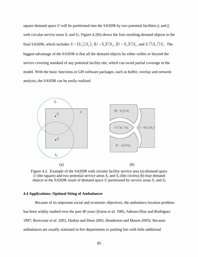
85

square demand space U will be partitioned into the SASDR by two potential facilities f1 and f2

with circular service areas S1 and S2. Figure 4.2(b) shows the four resulting demand objects in the

final SASDR, which includes ( )21 SSU − , ( ) 21 SSU − , ( ) 12 SSU − , and 21 SSU . The

biggest advantage of the SASDR is that all the demand objects lie either within or beyond the

service covering standard of any potential facility site, which can avoid partial coverage in the

model. With the basic functions in GIS software packages, such as buffer, overlay and network

analysis, the SASDR can be easily realized.

(a) (b)

Figure 4.2. Example of the SASDR with circular facility service area (a) demand space U (the square) and two potential service areas S1 and S2 (the circles) (b) four demand objects in the SASDR result of demand space U partitioned by service areas S1 and S2

4.4 Applications: Optimal Siting of Ambulances

Because of its important social and economic objectives, the ambulance location problem

has been widely studied over the past 40 years (Eaton et al. 1985, Adenso-Díaz and Rodríguez

1997, Brotcorne et al. 2003, Daskin and Dean 2005, Henderson and Mason 2005). Because

ambulances are usually stationed in fire departments or parking lots with little additional

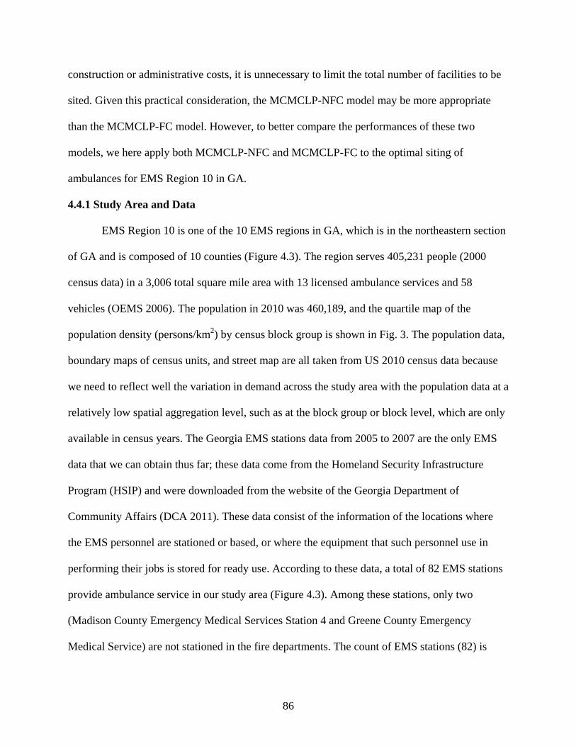
86

construction or administrative costs, it is unnecessary to limit the total number of facilities to be

sited. Given this practical consideration, the MCMCLP-NFC model may be more appropriate

than the MCMCLP-FC model. However, to better compare the performances of these two

models, we here apply both MCMCLP-NFC and MCMCLP-FC to the optimal siting of

ambulances for EMS Region 10 in GA.

4.4.1 Study Area and Data

EMS Region 10 is one of the 10 EMS regions in GA, which is in the northeastern section

of GA and is composed of 10 counties (Figure 4.3). The region serves 405,231 people (2000

census data) in a 3,006 total square mile area with 13 licensed ambulance services and 58

vehicles (OEMS 2006). The population in 2010 was 460,189, and the quartile map of the

population density (persons/km2) by census block group is shown in Fig. 3. The population data,

boundary maps of census units, and street map are all taken from US 2010 census data because

we need to reflect well the variation in demand across the study area with the population data at a

relatively low spatial aggregation level, such as at the block group or block level, which are only

available in census years. The Georgia EMS stations data from 2005 to 2007 are the only EMS

data that we can obtain thus far; these data come from the Homeland Security Infrastructure

Program (HSIP) and were downloaded from the website of the Georgia Department of

Community Affairs (DCA 2011). These data consist of the information of the locations where

the EMS personnel are stationed or based, or where the equipment that such personnel use in

performing their jobs is stored for ready use. According to these data, a total of 82 EMS stations

provide ambulance service in our study area (Figure 4.3). Among these stations, only two

(Madison County Emergency Medical Services Station 4 and Greene County Emergency

Medical Service) are not stationed in the fire departments. The count of EMS stations (82) is

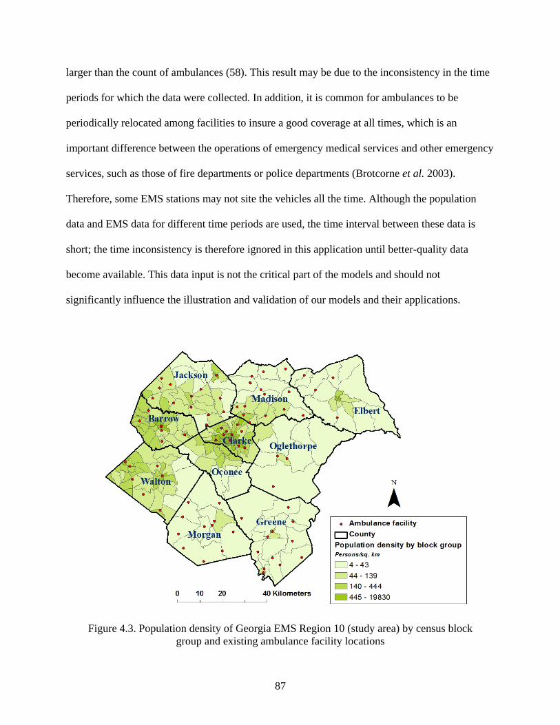
87

larger than the count of ambulances (58). This result may be due to the inconsistency in the time

periods for which the data were collected. In addition, it is common for ambulances to be

periodically relocated among facilities to insure a good coverage at all times, which is an

important difference between the operations of emergency medical services and other emergency

services, such as those of fire departments or police departments (Brotcorne et al. 2003).

Therefore, some EMS stations may not site the vehicles all the time. Although the population

data and EMS data for different time periods are used, the time interval between these data is

short; the time inconsistency is therefore ignored in this application until better-quality data

become available. This data input is not the critical part of the models and should not

significantly influence the illustration and validation of our models and their applications.

Figure 4.3. Population density of Georgia EMS Region 10 (study area) by census block

group and existing ambulance facility locations

88

4.4.2 Tasks

To test the application of the MCMCLP for emergency services, a total of 58 ambulances

will be allocated to maximize the covered allocated demands within 8-min driving distance from

the facilities. The locations of 82 existing EMS stations are regarded as the potential facility sites.

The demands are represented by the census population in 2010 by census block group. To ensure

the existence of a feasible solution to the problem, we define the capacity of each ambulance as

8000 persons so that 58 ambulances have total capacity of 464,000, which exceeds the total

demand of 460,189. We assume that the capacity of 8000 persons per ambulance can meet the

requirement of the average response time to the calls for service in this region. In the MCMCLP-

NFC model, the 58 vehicles could be allocated to, at most, 58 facility sites. In the MCMCLP-FC

model, only 20 potential facility sites will be chosen, and the 58 vehicles will be allocated to

these 20 sites. ArcGISTM v9.3.1 is used to realize the SASDR. Programming with Visual Basic

for Applications (VBA) for ArcObjects in ArcGISTM v9.3.1 is used to structure the optimization

model files. The optimization problems are then solved using the commercial mixed integer

programming (MIP) software package CPLEX v12.2. All analyses are performed on a personal

computer equipped with an Intel Core Quad 2.4 GHz CPU and 3 GB of RAM.

4.4.3 Results

4.4.3.1 Realization of SASDR

In the realization of SASDR, three types of roads are used to create the road network and

then to create the 8-min service area for each potential facility site. The information for roads is

listed in Table 4.1 and includes the MAF/TIGER Feature Class Codes (MTFCC) defined in the

census data, road descriptions and hypothetical speed limits. Figure 4.4 shows the road network

in the study area.

89

Table 4.1. Information for roads

MTFCC Description Speed limit(miles/hour)

S1100 Primary Road 70 S1200 Secondary Road 55 S1400 Local Neighborhood Road,

Rural Road, City Street 40

Figure 4.4. Road network in EMS Region 10 in GA

After the road network is created, a service layer that includes the 8-min service polygons

for the 82 potential facility sites is created from the road network using the network-analysis

functions in ArcGIS (Figure 4.5). The white areas indicate that no vehicles can reach these

locations within 8 minutes from any potential facility location. Each service polygon was

identified by the ID of its corresponding facility site.

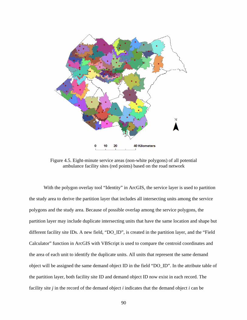
90

Figure 4.5. Eight-minute service areas (non-white polygons) of all potential

ambulance facility sites (red points) based on the road network

With the polygon overlay tool “Identity” in ArcGIS, the service layer is used to partition

the study area to derive the partition layer that includes all intersecting units among the service

polygons and the study area. Because of possible overlap among the service polygons, the

partition layer may include duplicate intersecting units that have the same location and shape but

different facility site IDs. A new field, “DO_ID”, is created in the partition layer, and the “Field

Calculator” function in ArcGIS with VBScript is used to compare the centroid coordinates and

the area of each unit to identify the duplicate units. All units that represent the same demand

object will be assigned the same demand object ID in the field “DO_ID”. In the attribute table of

the partition layer, both facility site ID and demand object ID now exist in each record. The

facility site j in the record of the demand object i indicates that the demand object i can be

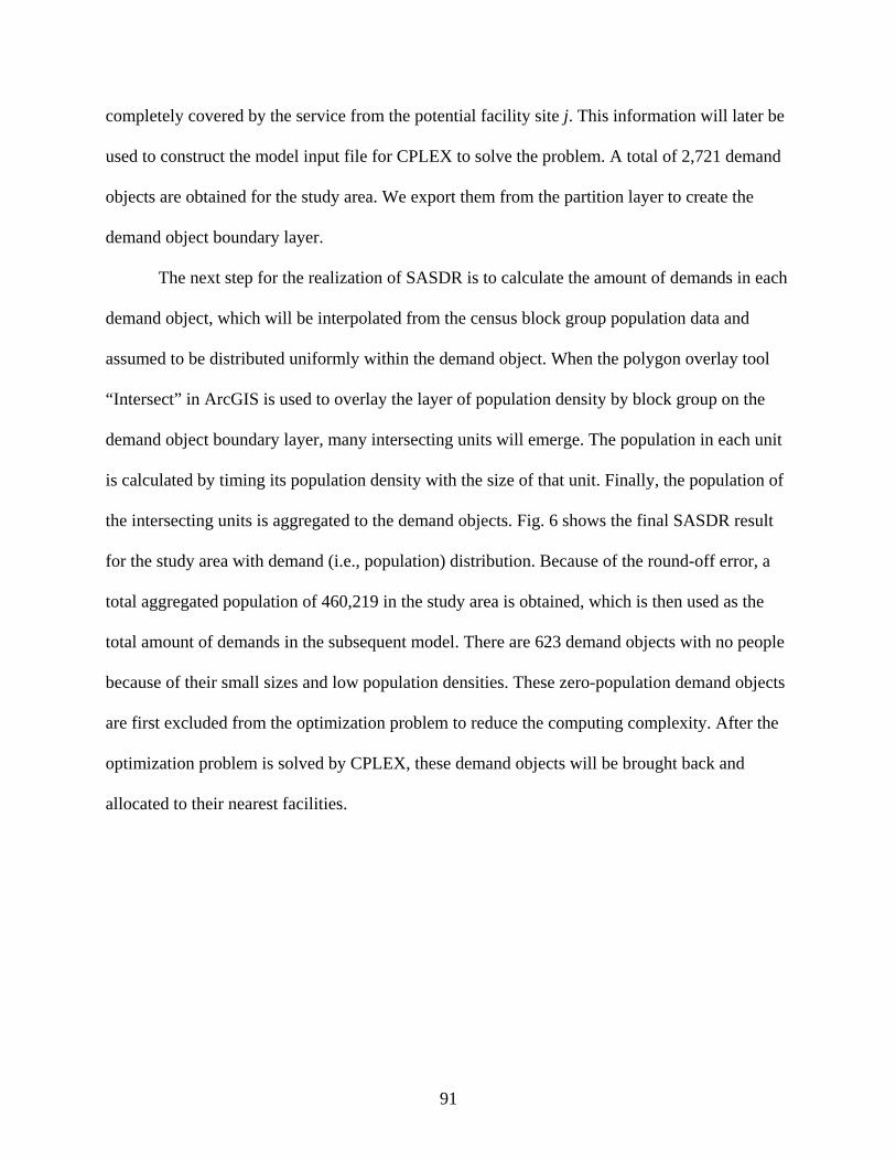
91

completely covered by the service from the potential facility site j. This information will later be

used to construct the model input file for CPLEX to solve the problem. A total of 2,721 demand

objects are obtained for the study area. We export them from the partition layer to create the

demand object boundary layer.

The next step for the realization of SASDR is to calculate the amount of demands in each

demand object, which will be interpolated from the census block group population data and

assumed to be distributed uniformly within the demand object. When the polygon overlay tool

“Intersect” in ArcGIS is used to overlay the layer of population density by block group on the

demand object boundary layer, many intersecting units will emerge. The population in each unit

is calculated by timing its population density with the size of that unit. Finally, the population of

the intersecting units is aggregated to the demand objects. Fig. 6 shows the final SASDR result

for the study area with demand (i.e., population) distribution. Because of the round-off error, a

total aggregated population of 460,219 in the study area is obtained, which is then used as the

total amount of demands in the subsequent model. There are 623 demand objects with no people

because of their small sizes and low population densities. These zero-population demand objects

are first excluded from the optimization problem to reduce the computing complexity. After the

optimization problem is solved by CPLEX, these demand objects will be brought back and

allocated to their nearest facilities.

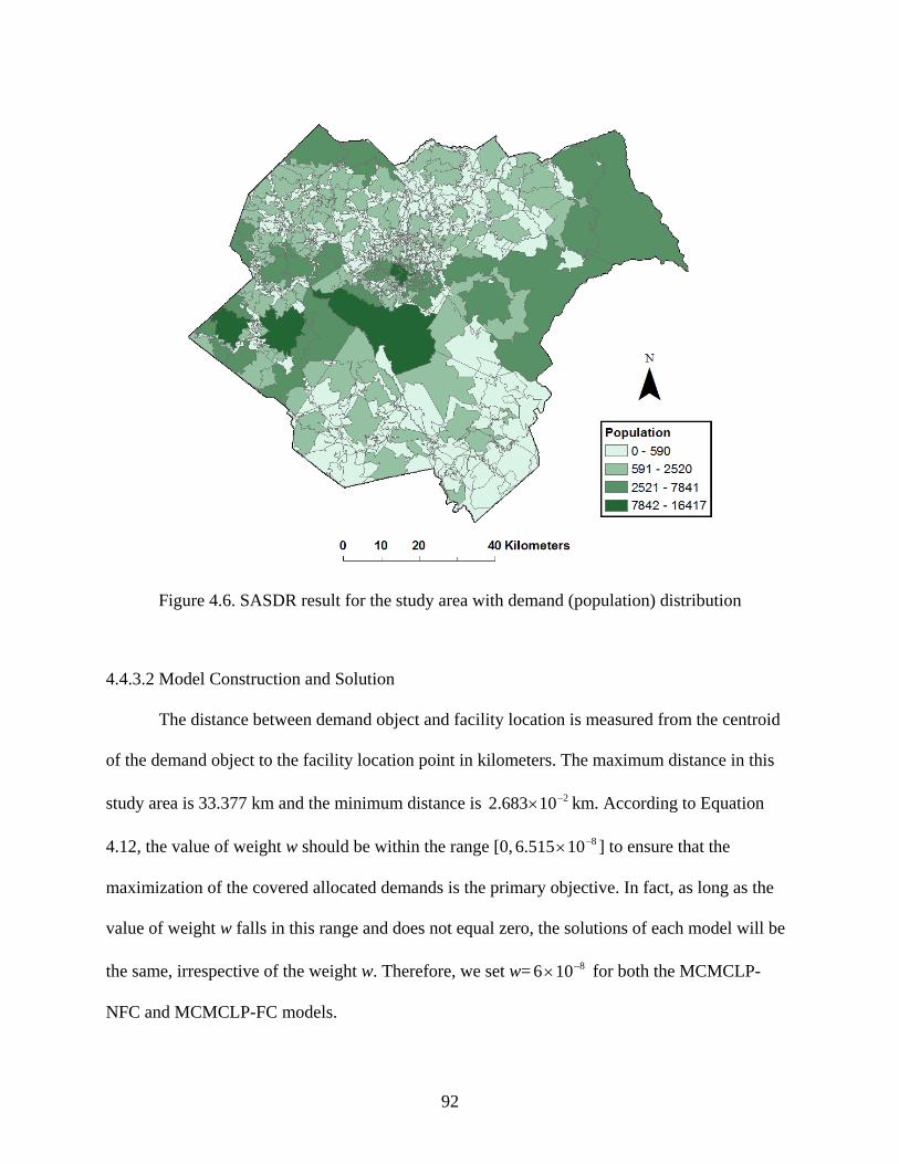
92

Figure 4.6. SASDR result for the study area with demand (population) distribution

4.4.3.2 Model Construction and Solution

The distance between demand object and facility location is measured from the centroid

of the demand object to the facility location point in kilometers. The maximum distance in this

study area is 33.377 km and the minimum distance is 210683.2 −× km. According to Equation

4.12, the value of weight w should be within the range [0, 810515.6 −× ] to ensure that the

maximization of the covered allocated demands is the primary objective. In fact, as long as the

value of weight w falls in this range and does not equal zero, the solutions of each model will be

the same, irrespective of the weight w. Therefore, we set w= 8106 −× for both the MCMCLP-

NFC and MCMCLP-FC models.

93

The model input files were constructed with the VBA program of ArcObjects in ArcGIS.

These models were then solved in CPLEX, which uses a branch-and-cut technique to find the

optimal solution (CPLEX Help 2011). The run time is 3,361 seconds for the MCMCLP-NFC

model and 706 seconds for the MCMCLP-FC model. The solutions obtained from CPLEX were

finally visualized as maps in ArcGIS.

Figure 4.7 shows the results of two MCMCLP models using the choropleth maps overlaid

with selected facility sites. In these maps, the facility and the demands allocated to it are

represented in the same colors, and larger facility symbols indicate more ambulances. With such

maps, the location-allocation patterns of the problem solution can be easily understood. For those

demand objects whose demands will be divided and allocated to more than one facility, the

strategy here is to split the demand object into multiple parts. For each facility that partially

serves the demand object, there is a part in the demand object trying to be close to that facility,

and its size is proportional to the percentage of demands served by that facility. In Figure 4.7(a),

in which the MCMCLP-NFC is applied, a total of 51 out of 82 potential sites are chosen to set up

the facilities, and 402,365 demands (87.4% of total demands) are covered within the 8-min

service covering standard. In Figure 4.7(b), in which the MCMCLP-FC is applied, 20 facilities

are required by the problem specification, and 358,477 demands (77.9% of total demands) are

covered within the service covering standard. As expected, the amount of the covered allocated

demands obtained by the MCMCLP-NFC is greater than that obtained by the MCMCLP-FC

because more facilities in the MCMCLP-NFC provide greater flexibility for siting the

ambulances. Because the proximity of the uncovered allocated demands to the facilities is

considered in both models (i.e., w= 8106 −× ), the demands allocated to a facility are generally

distributed more compactly and more continuous than those in the models with w=0 (results not

94

shown). However, the allocations of many facilities are still dispersed into several parts that may

be far away from one another. For example, there are two major demand patches with varied

sizes (filled with diagonals) allocated to the facility at site 13 in Figure 4.7(a). One reason for

this allocation is that the primary objective of the models is to maximize the covered allocated

demands instead of the proximity of the uncovered allocated demands to the facilities. The

splitting operation of the demand objects to represent the partial coverage could also cause the

noncontinuous demand allocations in the maps. Because of the smaller number of facilities

established, the MCMCLP-FC shows a more compact and continuous distribution of the

demands than the MCMCLP-NFC shows.

Table 4.2 shows the counts of the facilities with varied numbers of ambulances in these

two models. The maximum number of ambulances in a facility is 3 (site 45 in Figure 4.7(a)) in

the MCMCLP-NFC model and 12 (site 35 in Figure 4.7(b)) in the MCMCLP-FC model.

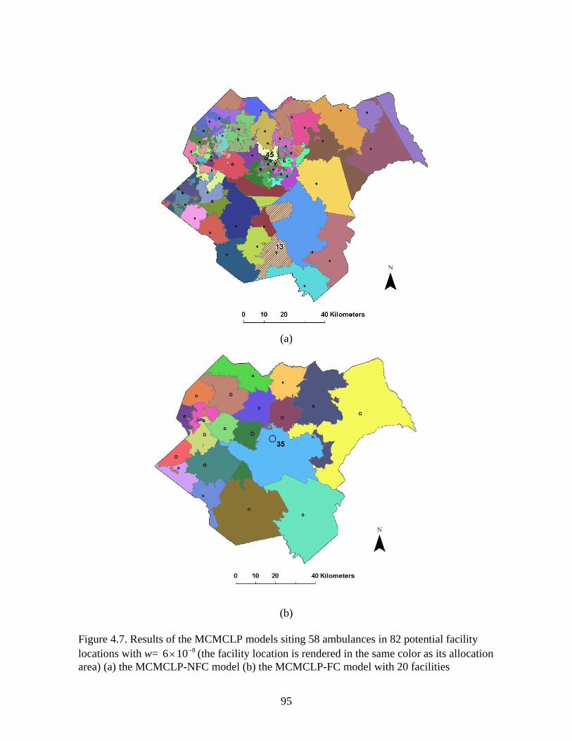
95

(a)

(b)

Figure 4.7. Results of the MCMCLP models siting 58 ambulances in 82 potential facility locations with w= 8106 −× (the facility location is rendered in the same color as its allocation area) (a) the MCMCLP-NFC model (b) the MCMCLP-FC model with 20 facilities

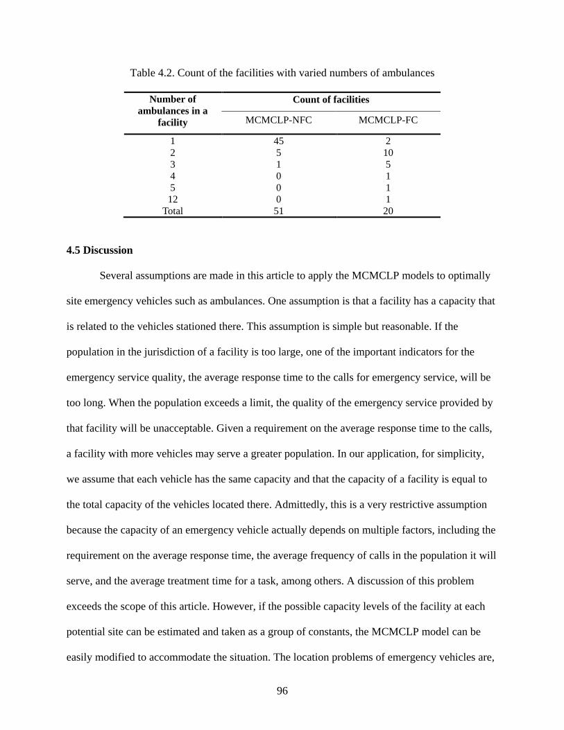
96

Table 4.2. Count of the facilities with varied numbers of ambulances

Number of ambulances in a

facility

Count of facilities

MCMCLP-NFC MCMCLP-FC

1 45 2 2 5 10 3 1 5 4 0 1 5 0 1 12 0 1

Total 51 20

4.5 Discussion

Several assumptions are made in this article to apply the MCMCLP models to optimally

site emergency vehicles such as ambulances. One assumption is that a facility has a capacity that

is related to the vehicles stationed there. This assumption is simple but reasonable. If the

population in the jurisdiction of a facility is too large, one of the important indicators for the

emergency service quality, the average response time to the calls for emergency service, will be

too long. When the population exceeds a limit, the quality of the emergency service provided by

that facility will be unacceptable. Given a requirement on the average response time to the calls,

a facility with more vehicles may serve a greater population. In our application, for simplicity,

we assume that each vehicle has the same capacity and that the capacity of a facility is equal to

the total capacity of the vehicles located there. Admittedly, this is a very restrictive assumption

because the capacity of an emergency vehicle actually depends on multiple factors, including the

requirement on the average response time, the average frequency of calls in the population it will

serve, and the average treatment time for a task, among others. A discussion of this problem

exceeds the scope of this article. However, if the possible capacity levels of the facility at each

potential site can be estimated and taken as a group of constants, the MCMCLP model can be

easily modified to accommodate the situation. The location problems of emergency vehicles are,

97

in reality, complex. The MCMCLP is a static model that does not consider the dynamic factors

such as the daily population movement. Accounting for such factors will be the focus of our

future work.

The MCLP has been proven to be nondeterministic polynomial time (NP)-hard (Megiddo

et al. 1981), which means that no algorithm has yet been discovered to solve it in polynomial

time in the worst case. As an extension to the MCLP, the MCMCLP is also NP-hard. Therefore,

the use of exact methods (e.g., enumeration or linear programming with branch-and-bound) to

solve a large-scale MCMCLP will be difficult. Seeking heuristic methods (e.g., genetic algorithm

or Lagrangian relaxation) is important for promoting the applications of the MCMCLP. A

potential heuristic method for solving the MCMCLP is a two-phase procedure, in which the

locations of the facilities and the demand allocation are first determined under the assumption

that the facilities are uncapacitated; the emergency vehicles are then allocated to each facility

depending on the allocated demands. We note that this two-phase procedure does not consider

that the second phase may change the demand allocation determined by the first phase, which

will cause the configuration of facility locations determined by the first phase to not necessarily

be the optimal solution for the whole problem.

Although model formulation and the optimization of algorithms are always the focus in

location modeling, many other aspects of the location problem, such as the representation for

spatial demands, also influence the accuracy of the modeling solutions and require attention. An

effective visualization of the problem solutions will be helpful in understanding the location-

allocation patterns and in making decisions by comparing different modeling results. One

problem that we need to address for our MCMCLP models in the future is how to better

represent in the map the demand objects served by multiple facilities.

98

In the MCMCLP model, GIS plays an important role. It is used to manage and organize

the spatial data, to realize the spatial demand representation, to help construct the model input

file for optimization software packages, and to visualize the problem solution with maps. In

addition to these important functions, GIS also facilitates theoretical advances in current location

science (Church 2002, Murray 2010).

4.6 Conclusion

The MCMCLP that we proposed in this article is an extension of the capacitated MCLP

to accommodate situations where the facilities to be sited have several possible capacity levels.

For the optimal siting of emergency vehicles, the MCMCLP considers the modular capacity

levels of a facility, the allocation of all demands, and the proximity of the uncovered allocated

demands to facilities. Two situations—the MCMCLP-NFC and the MCMCLP-FC—can be used

depending on the circumstances of the facility. In cases where the cost of a facility is low and

maximization of the covered allocated demands is the main purpose, such as establishing bases

for ambulances that are not always based in a building but are often at a very rudimentary

location such as a parking lot (Brotcorne et al. 2003), the MCMCLP-NFC may be more useful

because more covered allocated demands are generally obtained than with the MCMCLP-FC. If

the cost of facilities is also an important consideration, such as with fire stations for fire trucks,

the MCMCLP-FC may be better because we can incorporate information about how many

facilities we can build in the location modeling.

99

References

Adenso-Díaz, B. & Rodríguez, F., 1997. A simple search heuristic for the mclp: Application to the location of ambulance bases in a rural region. Omega, 25 (2), 181-187.

Balcik, B. & Beamon, B.M., 2008. Facility location in humanitarian relief. International Journal of Logistics: Research & Applications, 11 (2), 101-121.

Bennett, V.L., Eaton, D.J. & Church, R.L., 1982. Selecting sites for rural health workers. Social Science & Medicine, 16 (1), 63-72.

Berman, O. & Krass, D., 2002. The generalized maximal covering location problem. Computers & Operations Research, 29 (6), 563-581.

Brotcorne, L., Laporte, G. & Semet, F., 2003. Ambulance location and relocation models. European Journal of Operational Research, 147 (3), 451-463.



Church, R.L., 2002. Geographical information systems and location science. Computers & Operations Research, 29 (6), 541-562.

Church, R.L., Stoms, D.M. & Davis, F.W., 1996. Reserve selection as a maximal covering location problem. Biological conservation, 76 (2), 105-112.

Correia, I. & Captivo, M.E., 2003. A lagrangean heuristic for a modular capacitated location problem. Annals of Operations Research, 122 (1), 141-161.

Cplex Help, 2011. Branch and cut [online]. http://www.iro.umontreal.ca/~gendron/IFT6551/CPLEX/HTML/usrcplex/solveMIP9.html#638133 [Accessed Access Date 2011].

http://www.iro.umontreal.ca/~gendron/IFT6551/CPLEX/HTML/usrcplex/solveMIP9.html#638133�


100

Current, J. & O'kelly, M., 1992. Locating emergency warning sirens. Decision Sciences, 23 (1), 221-234.


Daskin, M. & Dean, L., 2005. Location of health care facilities. Operations Research and Health Care, 43-76.

Dca, 2011. Data and maps for planning [online]. http://www.georgiaplanning.com/dataforplanning.asp [Accessed Access Date 2011].

Eaton, D.J., Daskin, M.S., Simmons, D., Bulloch, B. & Jansma, G., 1985. Determining emergency medical service vehicle deployment in austin, texas. Interfaces, 96-108.

Griffin, P.M., Scherrer, C.R. & Swann, J.L., 2008. Optimization of community health center locations and service offerings with statistical need estimation. IIE Transactions, 40 (9), 880-892.

Haghani, A., 1996. Capacitated maximum covering location models: Formulations and solution procedures. Journal of advanced transportation, 30 (3), 101-136.

Henderson, S. & Mason, A., 2005. Ambulance service planning: Simulation and data visualisation. Operations Research and Health Care, 77-102.

Indriasari, V., Mahmud, A.R., Ahmad, N. & Shariff, A.R.M., 2010. Maximal service area problem for optimal siting of emergency facilities. International Journal of Geographical Information Science, 24 (2), 213-230.

Liao, K. & Guo, D., 2008. A clustering based approach to the capacitated facility location problem. Transactions in GIS, 12 (3), 323-339.


Murray, A.T., 2010. Advances in location modeling: Gis linkages and contributions. Journal of geographical systems, 12 (3), 335-354.

http://www.georgiaplanning.com/dataforplanning.asp�

101

Murray, A.T. & Gerrard, R.A., 1997. Capacitated service and regional constraints in location-allocation modeling. Location Science, 5 (2), 103-118.

Murray, A.T. & O'kelly, M.E., 2002. Assessing representation error in point-based coverage modeling. Journal of geographical systems, 4 (2), 171-191.

Oems, 2006. Office of emergency medical services/trauma operating report.

Pirkul, H. & Schilling, D.A., 1991. The maximal covering location problem with capacities on total workload. Management Science, 37 (2), 233-248.

Ratick, S.J., Osleeb, J.P. & Hozumi, D., 2009. Application and extension of the moore and revelle hierarchical maximal covering model. Socio-Economic Planning Sciences, 43 (2), 92-101.

Tong, D. & Murray, A.T., 2009. Maximising coverage of spatial demand for service. Papers in regional science, 88 (1), 85-97.

Verter, V. & Lapierre, S.D., 2002. Location of preventive health care facilities. Annals of Operations Research, 110 (1), 123-132.

Yin, P. & Mu, L., 2011. Service area spatial demand representation in maximal coverage modeling. Manuscript submitted for publication.

102

CHAPTER 5

AN EMPIRICAL COMPARISON OF SPATIAL DEMAND REPRESENTATIONS IN

MAXIMAL COVERAGE MODELING4

4 Yin, P and Mu, L. To be submitted to Environment and Planning B.

103

Abstract

Operationally representing spatial demand is necessary to apply location models to

planning processes and closely related to the efficiency of modeling solutions. A spatial demand

representation should not only be able to minimize representation error, but also keep the

complexity of model as low as possible. Most of the current research, however, is primarily

focused on assessing and reducing/eliminating representation error while ignoring the

complexity of modeling associated with demand representation. In this study, we use expressions

of set theory to formulize a polygon-overlay-based demand representation called service area

spatial demand representation (SASDR). Using the maximal covering location problem (MCLP)

as an example, we empirically compare SASDR to widely-used point-based and regular-area-

based demand representations in terms of both problem complexity and representation error. Our

study shows that, although use of SASDR can eliminate some errors associated with other

demand representations, problem complexity with SASDR could become extremely high with

the increase of potential facility sites, which could become computationally intractable for exact

methods in current optimization software. Point-based demand representation with fine

granularity sometimes is a good alternative to SASDR because it can provide similarly effective

modeling solutions while avoiding extensive computation in GIS for the realization of SASDR.

Regular-area-based demand representation is not strongly recommended based on its poor

performance compared to the point-based demand representation with a similar problem

complexity.

Keywords: MCLP, Spatial demand representation, Representation error, Problem complexity,

GIS

104

5.1 Introduction

The fact that different scale- and/or unit-definitions in geographic analyses produce

different results is known as the modifiable areal unit problem (MAUP) (Openshaw and Taylor

1981). The MAUP is important not only in general areas of geographic analysis, but also in

location modeling where the MAUP is manifested in aggregation and representation errors

(Cromley et al. 2012). There has been a long history of study on aggregation error in location

modeling including p-median problems and covering location problems (Hillsman and Rhoda

1978, Goodchild 1979, Current and Schilling 1987, Daskin et al. 1989, Current and Schilling

1990, Hodgson and Neuman 1993, Bowerman et al. 1999, Francis et al. 2009, Cromley et al.

2012). More recently, representation error in location modeling, especially covering location

models, has started to receive more attention (Murray and O'Kelly 2002, Murray et al. 2008,

Tong and Murray 2009, Cromley et al. 2012).

For covering location modeling, it is common to assume that aggregated or continuous

spatial demand is concentrated on a set of points or uniformly distributed within areal units. With

respect to these point-based and area-based demand representations, there are several studies

focusing on assessing the associated representation errors (Murray and O'Kelly 2002, Murray et

al. 2008). Several other studies tried to reduce or eliminate the representation errors by new

covering model formulations (Murray 2005, Tong and Murray 2009). Different from the

traditional area-based representations using census units or regular polygons, such as triangles or

rectangles, as demand objects, Cromley et al. (2012) proposed a new area-based demand

representation that partitions a continuous demand space using polygon overlay methods into a

set of areal units called the least common demand coverage units (LCDCUs). This representation

105

approach, without complicated model formulations, could reduce or eliminate some errors

associated with the traditional point-based and area-based representations.

Current studies with respect to spatial demand representations primarily focus on the

evaluation of representation errors and how to reduce or eliminate these errors. However, the

complexity of problems associated with demand representations is rarely discussed. Many

covering location models, such as the maximal covering location problem (MCLP), have been

proven to be nondeterministic polynomial time (NP)-hard (Megiddo et al. 1981), which means

that no algorithm has been discovered yet to solve it in polynomial time in the worst case.

Actually, the size of a covering location problem is highly related to the demand representation it

adopts. Therefore, even if a demand representation approach may theoretically reduce or

eliminate some representation errors in a problem, it probably could make the problem difficult,

if not impossible, to solve using exact methods in current optimization software. Relying on

some heuristic algorithms to solve such a complicated problem may introduce other errors in

modeling results.

As Cromley et al.’s (2012) spatial demand representation with LCDCUs is based on the

service area of a facility at each potential facility site, we define this representation as service

area spatial demand representation (SASDR). In this paper, we use the MCLP as an example to

empirically compare SASDR to the traditional point-based and regular-area-based

representations where both representation error and problem complexity are simultaneously

considered. Specifically, we evaluate problem complexity associated with these three types of

demand representations and compare their representation errors given similar degrees of problem

complexity. This comparison is expected to provide some insight on how to choose appropriate

demand representations in practical applications. Although the question of how to realize

106

SASDR with GIS was briefly described in texts by Cromley et al. (2012), it is worth formulizing

the process of its realization for better preciseness and clarity. In the following two sections,

more details about representation error and problem complexity in the MCLP are reviewed. Next,

the formulization of SASDR is given and explained. Experimental designs for understanding the

problem complexity and modeling errors associated with the three types of demand

representations are then described, followed by the experimental results and discussions. Finally,

some conclusions are offered.

5.2 Representation Error in Covering Location Modeling

In covering location modeling, aggregation and representation errors are related but

fundamentally different. Murray and O’Kelly (2002) have noted that the aggregation of spatial

information assumes there is one true lowest level of data. For example, the population at any

higher level in the census hierarchy is an instance of the aggregation of the population at any

lower level such as the census block level. Aggregation error occurs in any analysis conducted

above the level of the individual or whenever a scale change occurs (Cromley et al. 2012).

Comparing to demand aggregation, demand representation usually has no such hierarchy as that

in census data. Individual demand is usually represented by the location point of that demand.

Any aggregated or continuous demand is often assumed to be concentrated on a set of points or

uniformly distributed within areal units. With different point or areal tessellations for

representing the same aggregated or continuous demand in a region, some modeling errors could

occur. Such representation error is usually measured by comparing modeling results with one

spatial demand representation to those with another at the same aggregation levels.

It is a long-held tradition that continuous demand is represented by a set of discrete

weighted points where the weight represents the amount of demand for service on that point.

107

Many location models including the MCLP were proposed based on this kind of demand

representation. Along with the development of GIS in location science, areal units have been

used to represent continuous demand due to the 2-dimensional nature of demand space and the

strong capability of GIS to manipulate 2-dimensional spatial objects (Miller 1996, Kim and

Murray 2008, Murray et al. 2008, Tong et al. 2009, Tong and Murray 2009, Alexandris and

Giannikos 2010). Figure 5.1 shows four examples of the traditional point-based and area-based

representations for the demand in a region with three polygons. In Figure 5.1(a), the demand in

each polygon is assumed to be concentrated on the centroid of that polygon or uniformally

distributed within that polygon. Figure 5.1(b) shows using a rectangle grid or its centroids to

represent the demand space where the demand in each rectangle is assumed uniformally

distributed or concentrated on its centroid. When the demand within each demand object cannot

be obtained directly, which is very common, it may need to be estimated using areal

interpolation techniques with other available demand data that have inconsistent boundaries of

units with the demand representation. Especially, intelligent areal interpolation methods, which

is based on the principles of dasymetric mapping, usually can provide better estimates of the

spatial heterogeneity of demand within areal units than simple areal interplation methods do

(Cromley et al. 2012).

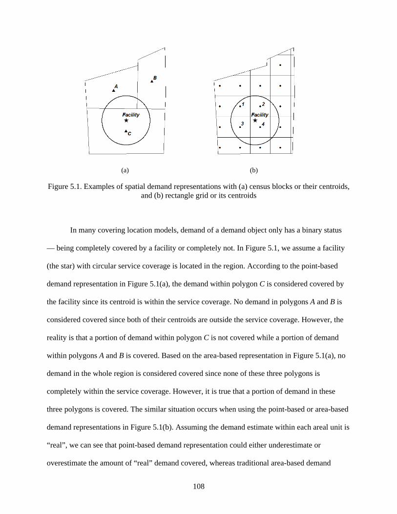
108

(a) (b)

Figure 5.1. Examples of spatial demand representations with (a) census blocks or their centroids, and (b) rectangle grid or its centroids

In many covering location models, demand of a demand object only has a binary status

— being completely covered by a facility or completely not. In Figure 5.1, we assume a facility

(the star) with circular service coverage is located in the region. According to the point-based

demand representation in Figure 5.1(a), the demand within polygon C is considered covered by

the facility since its centroid is within the service coverage. No demand in polygons A and B is

considered covered since both of their centroids are outside the service coverage. However, the

reality is that a portion of demand within polygon C is not covered while a portion of demand

within polygons A and B is covered. Based on the area-based representation in Figure 5.1(a), no

demand in the whole region is considered covered since none of these three polygons is

completely within the service coverage. However, it is true that a portion of demand in these

three polygons is covered. The similar situation occurs when using the point-based or area-based

demand representations in Figure 5.1(b). Assuming the demand estimate within each areal unit is

“real”, we can see that point-based demand representation could either underestimate or

overestimate the amount of “real” demand covered, whereas traditional area-based demand

109

representation could underestimate the amount of “real” demand covered. Such underestimation

or overestimation will lead to modeling errors in both the total amount of covered demand

estimated by the objective functions of models and the configuration of facilities given by the

decision variables in model results.

Based on the discussions by Casillas (1983) and Cromley et al. (2012), representation

error is defined as the difference between the objective function values optimized for the same

study area with two different demand representations. We use Cromley et al.’s (2012)

terminology and consider the following notation:

fa is an objective function using representation a

fb is an objective function using representation b

xa is the optimal solution to the problem using representation a

xb is the optimal solution to the problem using representation b

Taking representation b as the reference, representation error is defined as follow:

( ) ( )( )bb

bbaa

xfxfxf

error tionRepresenta][ −

= Equation 5.1

Representation error can be decomposed into cost error and optimality error. Cost error is the

difference between the objective function values of the same solution measured with two

different demand representations, which is shown as follow:

( ) ( )( )bb

abaa

xfxfxf

error Cost][ −

= Equation 5.2

110

Optimality error is the difference between the objective function values of two optimal solutions

measured with the same demand representation. It is defined as follow:

( ) ( )( )bb

bbab

xfxfxf

error Optimality][ −

= Equation 5.3

5.3 The MCLP Model and Problem Complexity

Given a covering standard for a service, such as maximum distance or travel time, the

objective of the MCLP is to locate a fixed number of facilities to provide service coverage for as

much spatial demand as possible. Consider the following notation:

I = the set of demand objects (i as demand object index)

J = the set of potential facility sites (j as facility site index)

dij= the travel distance or time from potential facility site j to demand object i

S = the distance or time beyond which a demand object is considered ‘uncovered’

wi = the demand for service at i

p = the total number of facilities to be located

=otherwise0

selected is sitefacility if1 jx j

=otherwise0

served)(or covered is demand if1 iyi

≤

=otherwise0

.., demand serving of capable is sitefacility if1 Sdeiija ij

ij

111

The formulation of the MCLP (Church and ReVelle (1974) is

Maximize ∑∈Ii

ii yw Equation 5.4

Subject to

iyxa

Jjijij ∀≥∑

∈

Equation 5.5

∑∈

=Jj

j px Equation 5.6

{ } jx j ∀∈ 1 0, Equation 5.7

{ } iyi ∀∈ 1 0, Equation 5.8

The objective Equation 5.4 seeks to maximally cover the amount of weighted demand.

Constraints 5.5 require that demand i can be covered only if at least one facility is located at the

sites where the service can cover demand i. Constraint 5.6 specifies the total number of facilities

to be located. Constraints 5.7 and 5.8 impose integrality conditions on decision variables.

The complexity of the MCLP problem mainly depends on the number of demand

constraints (Equation 5.5) and the number of integrality constraints on decision variables

(Equation 5.7) and (Equation 5.8). For each demand object (e.g., point or areal unit), if its

demand weight is larger than 0 and it can be covered by a facility at a potential location, there

will be a demand constraint and an integrality constraint associated with this demand object in

the MCLP model. Each potential facility site also contributes an integrality constraint to the

model. Therefore, the complexity of the MCLP problem is highly related with the spatial demand

representation and the number of potential facility sites in an application. When using census

112

units or their centroids to represent demand, the number of demand objects is equal to the

number of census units in the study area. However, when using point grid or regular area grid to

represent demand, the number of demand objects depends on the grid design which is often

arbitrary.

In applications of the MCLP model, the size of census unit or regular areal unit for

demand representation is usually smaller than the service coverage of a facility for better

accuracy of modeling results. Analysis based on a demand representation with finer granularity

(i.e., smaller size of demand object) also is expected to lead to smaller representation errors since

more complete demand objects can be covered within service coverage of a facility. With respect

to predefined potential facility sites, we need to consider multiple factors including cost, site

availability, proximity to demand, access to other services, etc., which may have large variability

in a region. More potential facility sites could provide more configurations of facilities to choose,

which in turn can improve the optimality on the amount of demand covered by a given number

of facilities. It is noted that, however, at the same time when more demand objects and potential

facility sites are used to improve modeling results, the model could become dramatically

complex and lead to a computational challenge for exact methods in current commercial

optimization software. Heuristic methods, such as genetic algorithms, provide alternative

approaches to solve such complex location problems. However, they cannot ensure optimal

solutions which could lead to other errors in modeling results, and sophisticated strategies for

heuristic algorithms and strong programming skills are also required.

5.4 Service Area Spatial Demand Representation

SASDR was originally described by Cromley et al. (2012) as an area-based demand

representation, with or without intelligent areal interpolation, used to be compared to census-

113

centroid-based demand representation in terms of representation and scale error. In this section,

we use expressions of set theory to formulize the realization of SASDR, which is easier to

understand and to be implemented in different GIS software packages. In addition, we discuss

both representation error and problem complexity of SASDR based on its concept.

The map overlay process has been used for approximately 50 years, and its multiple

forms are important spatial analysis methods in GIS (McHarg and American Museum of Natural

History. 1969, Longley et al. 2005). SASDR is based on one of the map overlay operations.

Considering two sets A (rectangle) and B (circle) in Figure 5.2(a), the overlay operation A▲B is

defined as below:

{ }φ≠−=∈= B} and XB,A{AIX|X B A ▲ Equation 5.9

where I is a two-member set in which, as shown in Figure 5.2(b), member BA − is the set of all

elements that are members of A but not members of B, and member BA is the set of all

elements that are members of both A and B. A▲B is the set whose members are those non-empty

members of I. Therefore, A▲B can be a two-member set { }BABA ,− when BA ≠ and

φ≠BA , be a one-member set { }BA − when φ≠A , BA ≠ and φ=BA , be a one-member

set { }BA when BA = and φ≠BA , or be the empty set φ when φ=A .

114

(a) (b)

Figure 5.2. Illustration of overlay operation A▲B: (a) set A and set B (b) the result from A▲B

For a set of sets C = {Ci, i= 1, 2, 3, …, n} and a set D, overlay operation C▲D is defined

as below:

( ) D C D Cn

1ii

=

= ▲▲ Equation 5.10

Therefore, C▲D is actually a set of sets consisting of all members of the sets obtained by

conducting the overlay operation on each member Ci of set C with set D.

Because the set of potential facility sites and the service standard are given in our case,

the service area at each potential facility site can then be determined. Consider the following

notation:

U = the whole demand space

Sj = the service area at potential facility site j (j = 1, 2, 3, …, m)

SASDR is defined as the partition of demand space U into a finite demand object set SA_DOS :

m321 S ... S S S USA_DOS ▲▲▲▲= Equation 5.11

115

Each element DOSSAD _∈ is defined as a demand object, also called LCDCU following

Cromley et al.’s (2012) terminology, that is disjointed with one other and UDDOSSAD

=∈

_

.

Figure 5.3(a) shows an example in which a rectangle demand space U will be partitioned

into a SASDR by two potential facility sites f1 and f2 with circular service areas S1 and S2. First,

demand space U is partitioned by service area S1, creating two demand objects

{ }11,▲ SUSU S U 1 −= (Figure 5.3(b)). Then, service area S2 is used to continue to partition

the demand space U. A total of four demand objects

( ) ( ) ( ) ( ){ }21212121▲▲ SSU,SSU,SSU,SSU S S U 21 −−−−= are created in the final

SASDR (Figure 5.3(c)). Demand objects ( ) 2SSU 1 − and ( ) 2SSU 1 can be completely

covered if a facility is located at site f1, and demand objects ( ) 21 SSU − and ( ) 2SSU 1 can

be completely covered if a facility is located at site f2. Neither of the services can completely or

partially cover demand object ( ) 21 SSU −− . Despite the simple circular shape demonstrated, the

facility service area could be any shape.

We can see that SASDR is fundamentally a simple map overlay-based approach.

Compared to point-based demand representations, it uses areal demand units that can reduce the

potential measurement and coverage errors caused by aggregating continuous demand to discrete

point demands. Compared to those traditional area-based demand representations using census

units or regular area grid, it has the advantage that all demand objects will either be completely

covered or not be covered by the service from any potential facility site. Without the partial

coverage problem, the modeling is more efficient than those in which the partial coverage needs

to be handled explicitly in models to reduce modeling errors, such as those proposed by Murray

(2005) and Tong and Murray (2009).

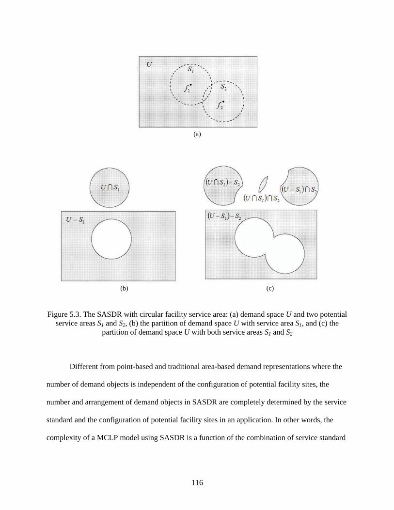
116

(a)

(b) (c)

Figure 5.3. The SASDR with circular facility service area: (a) demand space U and two potential service areas S1 and S2, (b) the partition of demand space U with service area S1, and (c) the

partition of demand space U with both service areas S1 and S2

Different from point-based and traditional area-based demand representations where the

number of demand objects is independent of the configuration of potential facility sites, the

number and arrangement of demand objects in SASDR are completely determined by the service

standard and the configuration of potential facility sites in an application. In other words, the

complexity of a MCLP model using SASDR is a function of the combination of service standard

117

and configuration of potential facility sites. This could be a problem when a high density of

potential facility sites is needed.

5.5 Experimental Design

Unlike previous studies where the comparisons of spatial demand representations only

focus on representation error, we also simultaneously consider problem complexity associated

with spatial demand representations. It is known that the increase of demand objects or potential

facility sites is expected to reduce representation error and improve the optimality of modeling

solutions. In our experiments, we mainly focus on the following two questions:

(1) How does the complexity of a problem using SASDR change when varying service

standard and configuration of potential facility sites?

(2) Given similar degrees of problem complexity, is there a large representation error

between SASDR and other types of demand representations including point-based

and traditional area-based approaches?

The study area in the experiments is the City of Decatur, Georgia which has an area of

approximately 4.2 square miles. The 2010 U.S. Census population data at the block level are

used to estimate the demand of each spatial object in all representations. To improve the

accuracy of the demand estimation, we use the 2010 land use data showing developed and

undeveloped areas as ancillary data and overly it on the census population data so that all

population are constrained within the developed areas. The 2010 land use data were downloaded

from the website of Atlanta Regional Commission (ARC 2012).

To have an understanding about question 1, we design three modes for potential facility

sites including one regular pattern and two irregular patterns as shown in Figure 5.4. Figure 5.4(a)

shows regular grid points with spacing R. Figure 5.4(b) shows the centroids of all census blocks,

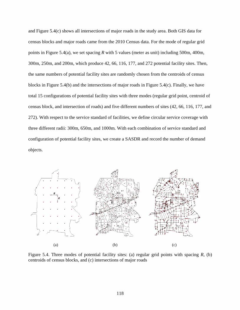
118

and Figure 5.4(c) shows all intersections of major roads in the study area. Both GIS data for

census blocks and major roads came from the 2010 Census data. For the mode of regular grid

points in Figure 5.4(a), we set spacing R with 5 values (meter as unit) including 500m, 400m,

300m, 250m, and 200m, which produce 42, 66, 116, 177, and 272 potential facility sites. Then,

the same numbers of potential facility sites are randomly chosen from the centroids of census

blocks in Figure 5.4(b) and the intersections of major roads in Figure 5.4(c). Finally, we have

total 15 configurations of potential facility sites with three modes (regular grid point, centroid of

census block, and intersection of roads) and five different numbers of sites (42, 66, 116, 177, and

272). With respect to the service standard of facilities, we define circular service coverage with

three different radii: 300m, 650m, and 1000m. With each combination of service standard and

configuration of potential facility sites, we create a SASDR and record the number of demand

objects.

(a)

(b)

(c)

Figure 5.4. Three modes of potential facility sites: (a) regular grid points with spacing R, (b) centroids of census blocks, and (c) intersections of major roads

119

For question 2, we use circular service coverage with a radius of 1000m in the

experiment. Among the 15 configurations of potential facility sites created in previous

experiment, we choose two configurations with 66 and 272 grid points and two configurations

with 66 and 272 centroids of census blocks. Therefore, there are total four SASDRs with the

combinations of one type of circular service coverage and four configurations of potential

facility sites. In all of these four situations, the whole study area can be covered by the service if

there are enough facilities located. For the traditional demand representations used to compare

with the SASDRs, we use four rectangle grids as the examples of traditional area-based demand

representation, and use the centroids of these rectangle grids as the examples of point-based

demand representation (Figure 5.5). By adjusting the spacing of the rectangle grid, we make the

numbers of demand objects in these four grid-rectangle-based and four grid-point-based demand

representations close to those in the four SASDRs. Finally, there are total four groups of

problems in this experiment for comparison, each of which includes three problems that have

different types of demand representations but similar degrees of problem complexity. The

number of facilities evaluated p in Equation 5.6 for all of the problems starts from 1 and

increases by 1 every time until the modeling reports 100% demand covered.

120

Figure 5.5. Examples of grid-point-based and grid- rectangle-based demand representations for comparison with SASDR

ArcGISTM v10 is used to realize the SASDR and its visualization. Programming with

Visual Basic for Applications (VBA) for ArcObjects in ArcGISTM v10 is used to structure the

optimization model file. The problems are solved using a commercial optimization package

CPLEX v12.2 that uses a Branch-and-Cut technique to search the optimal solution (CPLEX Help

2011). All analyses are carried out on a personal computer with Intel Core Quad 2.4 GHz CPU

and 3 GB RAM.

5.6 Results and Discussions

5.6.1 Problem Complexity with SASDR

Table 5.1 summarizes the numbers of demand objects in 45 SASDRs with different

combinations of service radius (SR) and configuration of potential facility sites. We can see that,

regardless of whether the pattern of potential facility sites is regular (grid point) or irregular

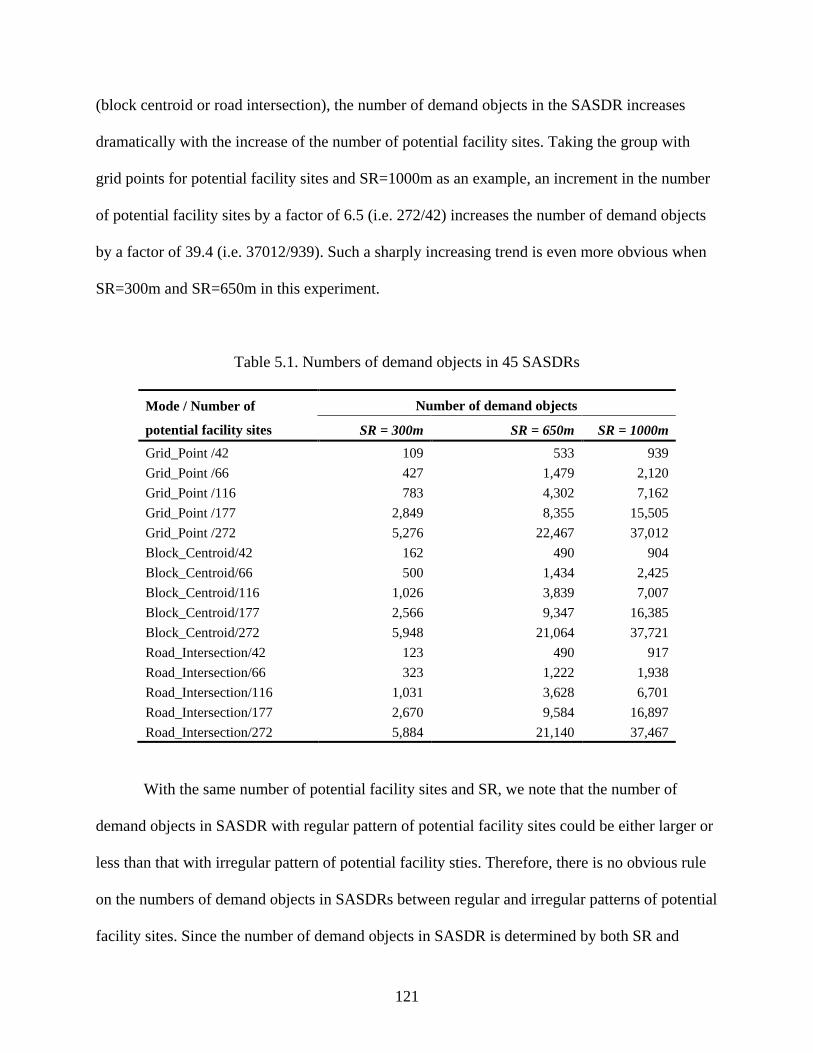
121

(block centroid or road intersection), the number of demand objects in the SASDR increases

dramatically with the increase of the number of potential facility sites. Taking the group with

grid points for potential facility sites and SR=1000m as an example, an increment in the number

of potential facility sites by a factor of 6.5 (i.e. 272/42) increases the number of demand objects

by a factor of 39.4 (i.e. 37012/939). Such a sharply increasing trend is even more obvious when

SR=300m and SR=650m in this experiment.

Table 5.1. Numbers of demand objects in 45 SASDRs

Mode / Number of

potential facility sites Number of demand objects

SR = 300m SR = 650m SR = 1000m Grid_Point /42 109 533 939 Grid_Point /66 427 1,479 2,120 Grid_Point /116 783 4,302 7,162 Grid_Point /177 2,849 8,355 15,505 Grid_Point /272 5,276 22,467 37,012 Block_Centroid/42 162 490 904 Block_Centroid/66 500 1,434 2,425 Block_Centroid/116 1,026 3,839 7,007 Block_Centroid/177 2,566 9,347 16,385 Block_Centroid/272 5,948 21,064 37,721 Road_Intersection/42 123 490 917 Road_Intersection/66 323 1,222 1,938 Road_Intersection/116 1,031 3,628 6,701 Road_Intersection/177 2,670 9,584 16,897 Road_Intersection/272 5,884 21,140 37,467

With the same number of potential facility sites and SR, we note that the number of

demand objects in SASDR with regular pattern of potential facility sites could be either larger or

less than that with irregular pattern of potential facility sties. Therefore, there is no obvious rule

on the numbers of demand objects in SASDRs between regular and irregular patterns of potential

facility sites. Since the number of demand objects in SASDR is determined by both SR and

122

configuration of potential facility sites, we use Site-Service Index to measure the degree of

clustering of potential facility sites at the scale defined by SR. Site-Service Index describes the

average number of potential facility sites within a circle with radius = 2SR and is defined as

follow:

( )N

SRdI Index Service-Site

N

i

N

jij∑∑ ≤

=2

Equation 5.12

where i and j are the indexes of potential facility sites, dij is the distance between potential

facility sites i and j, N is the total number of potential facility sites in a study region, and I(·) is an

indicator function. We define the ratio of the total number of demand objects in SASDR to N as

demand object density. Figure 5.6 shows the scatter plot of Site-Service Index and demand

object density for the 45 SASDRs in our experiment. We can see there is a strong linear

relationship between these two measures for either regular or irregular patterns of potential

facility sites. The R2 is 0.998 among all of the three modes of potential facility sites. This linear

relationship can be used to predict the number of demand objects in SASDR with circular service

coverage, which equals to the multiplication of demand object density and N. Given a fixed

study area and a SR, when N increases to some degree, the spatial pattern of potential facility

sites start to become more and more clustered, and then Site-Service Index increases accordingly,

which indicates an increase of the demand object density based on the linear relationship.

Therefore, both increases of N and demand object density will make the total number of demand

objects rise quickly.

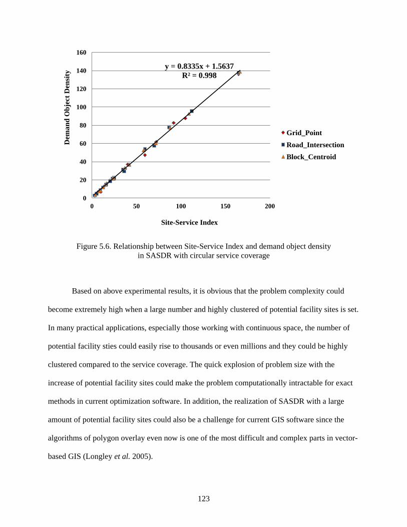
123

Figure 5.6. Relationship between Site-Service Index and demand object density

in SASDR with circular service coverage

Based on above experimental results, it is obvious that the problem complexity could

become extremely high when a large number and highly clustered of potential facility sites is set.

In many practical applications, especially those working with continuous space, the number of

potential facility sties could easily rise to thousands or even millions and they could be highly

clustered compared to the service coverage. The quick explosion of problem size with the

increase of potential facility sites could make the problem computationally intractable for exact

methods in current optimization software. In addition, the realization of SASDR with a large

amount of potential facility sites could also be a challenge for current GIS software since the

algorithms of polygon overlay even now is one of the most difficult and complex parts in vector-

based GIS (Longley et al. 2005).

y = 0.8335x + 1.5637 R² = 0.998

0

20

40

60

80

100

120

140

160

0 50 100 150 200

Dem

and

Obj

ect D

ensi

ty

Site-Service Index

Grid_Point Road_Intersection Block_Centroid

124

5.6.2 Comparison in Representation Error

Given SR=1000m, Table 5.2 shows the numbers of demand objects in the four groups of

problems with three types of demand representations for comparison. In the SASDRs in this

experiment, the configurations of 66 potential facility sites lead to about 2,000 demand objects,

while 272 potential facility sites lead to over 30,000 demand objects. The different numbers of

demand objects also reflect the degrees of granularity of the demand representations. Since the

difference in the number of demand objects within each group is less than 0.1%, and the same

configuration of potential facility sites is used for the three problems in each group, the problems

in each group for comparison have similar degrees of complexity.

Table 5.2. Numbers of demand objects in all demand representations for comparison

Mode / Number of potential facility sites

Number of demand objects SASDR Point or rectangle grid Difference

Grid_Point /66 2,120 2,120 0.00% Grid_Point /272 37,012 36,988 0.06% Block_Centroid/66 2,425 2,426 0.04% Block_Centroid/272 37,721 37,715 0.02%

Table 5.3 shows the minimum numbers of facilities reported by the objective functions to

cover 100% demand in the study area. As expected, more potential facility sites usually need

fewer facilities to cover the same demand space. We also notice that one more facility is needed

for the grid-rectangle demand representation than other two demand representations when using

66 block centroids as the potential facility sites. It is mainly due to the underestimation of “real”

covered demand by grid-rectangle demand representation.

125

Table 5.3. Minimum numbers of facilities reported by models for covering 100% demand

Mode / Number of potential facility sites

Minimum number of facilities for 100% demand coverage SASDR Point grid Rectangle grid

Grid_Point /66 8 8 8 Grid_Point /272 7 7 7 Block_Centroid/66 9 9 10 Block_Centroid/272 7 7 7

Figure 5.7 shows the percentages of covered demand reported by the MCLP models with

three types of demand representations for four configurations of potential facility sites. Both of

the regular and irregular configurations of potential facility sites show similar characteristics on

the percentage of covered demand. When there are only 66 potential facility sites, the grid-

rectangle demand representations lead to less percentages of covered demand than the SASDRs

and point-based demand representations do. When the number of potential facility sties increases

to 272, all three demand representations have very similar percentages of covered demand.

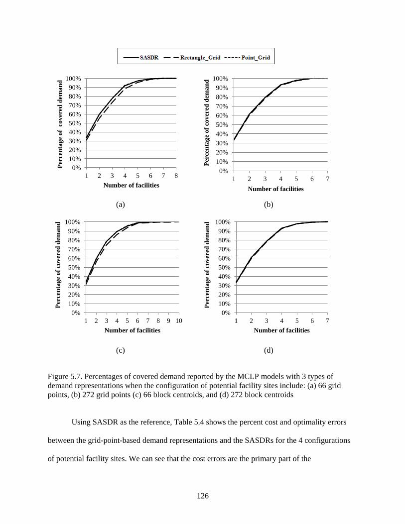
126

(a) (b)

(c) (d)

Figure 5.7. Percentages of covered demand reported by the MCLP models with 3 types of demand representations when the configuration of potential facility sites include: (a) 66 grid points, (b) 272 grid points (c) 66 block centroids, and (d) 272 block centroids

Using SASDR as the reference, Table 5.4 shows the percent cost and optimality errors

between the grid-point-based demand representations and the SASDRs for the 4 configurations

of potential facility sites. We can see that the cost errors are the primary part of the

0% 10% 20% 30% 40% 50% 60% 70% 80% 90%

100%

1 2 3 4 5 6 7 8

Perc

enta

ge o

f co

vere

d de

man

d

Number of facilities

0% 10% 20% 30% 40% 50% 60% 70% 80% 90%

100%

1 2 3 4 5 6 7

Perc

enta

ge o

f cov

ered

dem

and


0% 10% 20% 30% 40% 50% 60% 70% 80% 90%

100%

1 2 3 4 5 6 7 8 9 10

Perc

enta

ge o

f cov

ered

dem

and


0% 10% 20% 30% 40% 50% 60% 70% 80% 90%

100%

1 2 3 4 5 6 7

Perc

enta

ge o

f cov

ered

dem

and


127

representation errors in each group. The magnitudes of the cost errors become smaller when

more demand objects (i.e., finer granularity of demand representation) are used. In addition, the

non-zero cost errors are either positive or negative, which is the same as what we expect that

point-based demand representation could either overestimate or underestimate covered demand.

Table 5.4 also shows that only a few non-zero optimality errors occur when 66 potential facility

sites are set with about 2000 demand objects. When 272 potential facility sites are used with over

30,000 demand objects, all optimality errors are 0. This observation shows that, with the

improvement of the granularity of demand representation, the differences generally become

smaller on the optimal configurations of facilities given by the MCLP models with point-based

demand representation and SASDR. We also notice that, when the number of demand objects is

small, the real 100% covered demand may be not reached when the models report 100% covered

demand, such as 8 facilities for the potential facility sites of 66 grid points and 9 facilities for the

potential facility sites of 66 block centroids in this experiment.

Table 5.4. Cost and optimality errors between grid-point-based demand representations and SASDRs

Grid_Point /66 (2120)

Grid_Point /272 (36988)

Block_Centroid/66 (2426)


p Cost Optimality Cost Optimality Cost Optimality Cost Optimality 1 -0.08% 0.00% -0.06% 0.00% 0.06% 0.00% 0.01% 0.00% 2 -0.03% 0.00% 0.05% 0.00% 0.12% 0.00% 0.00% 0.00% 3 0.24% 0.00% -0.02% 0.00% 0.12% -0.07% 0.02% 0.00% 4 0.39% 0.00% 0.00% 0.00% 0.26% -0.12% 0.02% 0.00% 5 0.14% 0.00% 0.00% 0.00% 0.14% 0.00% -0.02% 0.00% 6 -0.02% 0.00% 0.00% 0.00% 0.04% 0.00% 0.01% 0.00% 7 0.00% 0.00% 0.00% 0.00% 0.07% 0.00% 0.00% 0.00% 8 0.02% -0.02% 0.01% 0.00% 9 0.03% -0.03%

Note: the number in the parentheses shows the number of demand objects in each demand representation

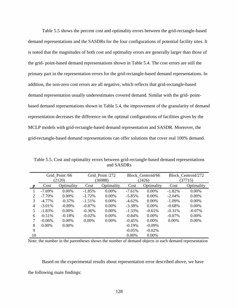
128

Table 5.5 shows the percent cost and optimality errors between the grid-rectangle-based

demand representations and the SASDRs for the four configurations of potential facility sites. It

is noted that the magnitudes of both cost and optimality errors are generally larger than those of

the grid- point-based demand representations shown in Table 5.4. The cost errors are still the

primary part in the representation errors for the grid-rectangle-based demand representations. In

addition, the non-zero cost errors are all negative, which reflects that grid-rectangle-based

demand representation usually underestimates covered demand. Similar with the grid- point-

based demand representations shown in Table 5.4, the improvement of the granularity of demand

representation decreases the difference on the optimal configurations of facilities given by the

MCLP models with grid-rectangle-based demand representation and SASDR. Moreover, the

grid-rectangle-based demand representations can offer solutions that cover real 100% demand.

Table 5.5. Cost and optimality errors between grid-rectangle-based demand representations and SASDRs

Grid_Point /66 (2120)

Grid_Point /272 (36988)



p Cost Optimality Cost Optimality Cost Optimality Cost Optimality 1 -7.69% 0.00% -1.85% 0.00% -7.61% 0.00% -1.82% 0.00% 2 -7.70% 0.00% -1.72% 0.00% -5.85% 0.00% -2.04% 0.00% 3 -4.77% -0.37% -1.51% 0.00% -4.62% 0.00% -1.09% 0.00% 4 -3.01% -0.89% -0.87% 0.00% -3.38% 0.00% -0.68% 0.00% 5 -1.83% 0.00% -0.36% 0.00% -1.33% -0.61% -0.31% -0.07% 6 -0.51% -0.18% -0.02% 0.00% -0.84% 0.00% -0.07% 0.00% 7 -0.06% 0.00% 0.00% 0.00% -0.45% 0.00% 0.00% 0.00% 8 0.00% 0.00% -0.19% -0.09% 9 -0.05% -0.02% 10 0.00% 0.00%

Note: the number in the parentheses shows the number of demand objects in each demand representation

Based on the experimental results about representation error described above, we have

the following main findings:

129

(1) SASDR and the traditional area-based demand representations (e.g., use of census

units or regular polygons as demand objects) can both offer solutions providing real

100% covered demand if the whole demand space can be covered by enough number

of facilities with a given configuration of potential facility sites. However, the

minimum number of needed facilities analyzed with the traditional area-based

demand representation could be larger than optimal solutions. Point-based demand

representation with coarse granularity is difficult to offer solutions that provide real

100% covered demand. However, the improvement of the granularity of point-based

demand representation could mitigate the problem.

(2) Given similar problem sizes and using SASDR as the reference, when the granularity

of demand representation is relatively coarse, the representation errors, including cost

and optimality errors, associated with both point-based and the traditional area-based

demand representations are obvious. However, when the granularity of demand

representation is fine, the representation errors could become very small, especially

the optimality errors. In that case, the model solutions about the configuration of

facilities could be equally effective no matter which type of demand representation is

used.

(3) When the degrees of granularity are close, grid-point-based demand representation

usually has better performance than grid-area-based demand representation in terms

of both cost and optimality error.

These main findings provide us some implications on how to choose appropriate spatial

demand representation in practical applications. When a small number of potential facility sites

is needed or there is a requirement on real 100% covered demand, SASDR is a good choice.

130

When the number of potential facility sites rises to a large number that could lead to a SASDR

with very fine granularity, using a point-based demand representation may be a good choice

based on the following considerations. If a SASDR results in a large problem size that, however,

is still solvable for exact methods in current optimization software, using a point-based demand

representation with similar problem complexity as an alternative can give similar modeling

solutions while avoiding extensive computation in GIS for the realization of SASDR. In point-

based demand representation, the number of demand points is independent of the configuration

of potential facility sites, which provides a flexible approach to balance problem complexity and

representation error. If a problem using SASDR is too complex to solve by exact methods in

current optimization software, it is possible to replace it by a point-based demand representation

with less number of demand objects that can be defined based on the capability of optimization

software. The loss of covered demand due to the representation errors could be compensated by

increasing the number of potential facility sites without a large increase of problem size.

Regular-area-based demand representation is not strongly recommended because, given similar

problem sizes, its performance is usually not as good as point-based demand representation and

it also needs spatial analysis functions in GIS to examine the topological relationship between

service coverage and each regular areal demand unit, which could be very time-consuming.

5.7 Conclusions

Spatial demand representation is an important topic in location modeling because it is

necessary for applying location models to the planning process and strongly associated with the

efficiency of modeling solutions. A spatial demand representation should not only be able to

minimize representation error but also need to keep the complexity of model as low as possible.

Most of current research, however, is primarily focusing on assessing and trying to reduce or

131

eliminate representation error while ignoring the complexity of model associated with demand

representation. In this paper, we use expressions of set theory to formulize SASDR that is a

polygon-overlay-based demand representation originally described by Cromley et al. (2012) and

also used for siting emergency vehicles by Yin and Mu (2012). Using the MCLP as an example,

we then empirically compare SASDR to widely-used point-based and regular-area-based demand

representations in terms of both problem complexity and representation error.

SASDR has several advantages including being able to offer solutions providing real 100%

covered demand and eliminating some errors associated with point-based and other area-based

demand representations. However, our study shows that, the complexity of problem with

SASDR could become extremely high when increasing the number and the degree of clustering

of potential facility sites. This problem could lead to a dilemma for many practical applications

where it is common to set a large number of potential facility sites for larger covered demand.

Many covering location problems themselves are nondeterministic polynomial time (NP)-hard

(Megiddo et al. 1981), which means that no algorithm has yet been discovered to solve it in

polynomial time in the worst case. Therefore, these problems using SASDR could become more

difficult, if not impossible, to solve by exact methods in current commercial optimization

software. In such cases, heuristic methods may be the only ways that however could introduce

other errors to modeling solutions and requires sophisticated strategies for algorithms and strong

programming skills. In addition, the realization of SASDR for a large number of potential facility

sites could be also a computational challenge for current GIS software.

The empirical comparisons of problems with similar degrees of complexity, but different

spatial demand representations, provide us some insight on how to choose appropriate spatial

demand representation in practical applications. Point-based demand representation sometimes is

132

a good alternative to SASDR when the problem with SASDR is too complex to solve by exact

methods in current optimization software.

As we know, point-based and regular-area-based demand representations can be very

flexible depending on the number and arrangement of demand objects as well as the shape of

areal unit. In this study, we only choose a limited number of point-based and regular-area-based

demand representations as examples to explore their characteristics in the MCLP modeling. Our

findings may not be able to be generalized well to all situations.

In addition, we need to notice that the MCLP has been extended to incorporate more

considerations to meet specific application requirements, such as the capacitated facility (Chung

et al. 1983, Current and Storbeck 1988, Haghani 1996) and the allocation of demand beyond the

covering standard in emergency service planning (Pirkul and Schilling 1991, Yin and Mu 2012).

In these variations of the MCLP, allocation of demand to facilities needs to be considered. The

aggregation and representation errors on demand allocation could be one topic of our research in

the future.

133

References

Alexandris, G. & Giannikos, I., 2010. A new model for maximal coverage exploiting gis capabilities. European Journal of Operational Research, 202 (2), 328-338.

Arc, 2012. Gis data and maps [online]. http://www.atlantaregional.com/info-center/gis-data-maps/gis-data [Accessed Access Date 2012].

Bowerman, R.L., Calamai, P.H. & Brent Hall, G., 1999. The demand partitioning method for reducing aggregation errors in p-median problems. Computers & Operations Research, 26 (10-11), 1097-1111.

Casillas, P., 1983. Data aggregation and the p-median problem in continuous space. In Ghosh, A. & Rushton, G. eds. Spatial analysis and location-allocation models. New York: Van Nostrand Reinhold, 327-344.



Cplex Help, 2011. Branch and cut [online]. http://www.iro.umontreal.ca/~gendron/IFT6551/CPLEX/HTML/usrcplex/solveMIP9.html#638133 [Accessed Access Date 2011].

Cromley, R.G., Lin, J. & Merwin, D.A., 2012. Evaluating representation and scale error in the maximal covering location problem using gis and intelligent areal interpolation. International Journal of Geographical Information Science, 26 (3), 495-517.


Current, J.R. & Schilling, D.A., 1987. Elimination of source a and b errors in p‐ median location problems. Geographical Analysis, 19 (2), 95-110.

http://www.atlantaregional.com/info-center/gis-data-maps/gis-data�

http://www.atlantaregional.com/info-center/gis-data-maps/gis-data�



134

Current, J.R. & Schilling, D.A., 1990. Analysis of errors due to demand data aggregation in the set covering and maximal covering location problems. Geographical Analysis, 22 (2), 116-126.

Daskin, M.S., Haghani, A.E., Khanal, M. & Malandraki, C., 1989. Aggregation effects in maximum covering models. Annals of Operations Research, 18 (1), 113-139.

Francis, R., Lowe, T., Rayco, M. & Tamir, A., 2009. Aggregation error for location models: Survey and analysis. Annals of Operations Research, 167 (1), 171-208.

Goodchild, M.F., 1979. The aggregation problem in location‐ allocation. Geographical Analysis, 11 (3), 240-255.

Haghani, A., 1996. Capacitated maximum covering location models: Formulations and solution procedures. Journal of advanced transportation, 30 (3), 101-136.

Hillsman, E.L. & Rhoda, R., 1978. Errors in measuring distances from populations to service centers. The Annals of Regional Science, 12 (3), 74-88.

Hodgson, M.J. & Neuman, S., 1993. A gis approach to eliminating source c aggregation error in p-meidan models. Computers & Operations Research.

Kim, K. & Murray, A.T., 2008. Enhancing spatial representation in primary and secondary coverage location modeling. Journal of Regional Science, 48 (4), 745-768.

Longley, P.A., Goodchild, M.F., Maguire, D.J. & Rhind, D.W., 2005. Geographic information systems and science, 2nd ed.: John Wiley & Sons, Ltd.

Mcharg, I.L. & American Museum of Natural History., 1969. Design with nature, 1st ed. Garden City, N.Y.,: Published for the American Museum of Natural History [by] the Natural History Press.


Miller, H.J., 1996. Gis and geometric representation in facility location problems. International Journal of Geographical Information Systems, 10 (7), 791-816.

135

Murray, A.T., 2005. Geography in coverage modeling: Exploiting spatial structure to address complementary partial service of areas. Annals of the Association of American Geographers, 95 (4), 761-772.

Murray, A.T. & O'kelly, M.E., 2002. Assessing representation error in point-based coverage modeling. Journal of geographical systems, 4 (2), 171-191.

Murray, A.T., O'kelly, M.E. & Church, R.L., 2008. Regional service coverage modeling. Computers & Operations Research, 35 (2), 339-355.

Openshaw, S. & Taylor, P.J., 1981. The modifiable areal unit problem. In Wrigley, N. & Bennett, R. eds. Quantitative geography: A british view. London and Boston: Routledge and Kegan Paul, 60-69.

Pirkul, H. & Schilling, D.A., 1991. The maximal covering location problem with capacities on total workload. Management Science, 37 (2), 233-248.

Tong, D., Murray, A. & Xiao, N., 2009. Heuristics in spatial analysis: A genetic algorithm for coverage maximization. Annals of the Association of American Geographers, 99 (4), 698-711.

Tong, D. & Murray, A.T., 2009. Maximising coverage of spatial demand for service. Papers in regional science, 88 (1), 85-97.

Yin, P. & Mu, L., 2012. Modular capacitated maximal covering location problem for the optimal siting of emergency vehicles. Applied Geography, 34 (0), 247-254.

136

CHAPTER 6

CONCLUSIONS

6.1 Summary and Conclusions

With increasing digital health data and environmental, socioeconomic, behavioral data

available, Geographic Information Systems (GIS) are receiving increased attention in public

health studies. This dissertation research mainly focuses on three aspects of health studies using

GIS and spatial analysis: spatial disease cluster detection, spatio-temporal disease mapping, and

health service planning. New methods or models are proposed and implemented with GIS in this

research to address an important problem in each of the three aspects.

With respect to the detection of spatial disease cluster, for the first time, our study

implements and tests Tango’s (2008) restricted likelihood ratio combined with Assunção et al.’s

(2006) dynamic Minimum Spanning Tree (dMST) search strategy to quickly detect disease

clusters in arbitrary shapes. To understand the performance of this redesigned hybrid method in

various situations, we design six cluster models and two non-cluster scenarios. These cluster

models consider different numbers of disease cases in a study area and various shapes of clusters.

The choice of the screening level α1 in restricted likelihood ratio is also explored in our

redesigned spatial scan statistic method (RSScan). Besides the metric of power, we propose

using the Kappa Index of Agreement (KIA) to evaluate and compare the performances of cluster

detection methods to identify the boundaries of clusters in order to avoid the effects due to the

different cluster model properties. Finally, we provide the application of our RSScan method in a

137

case of detecting the cluster of lung cancer incidence in Georgia for the period 1998-2005. The

experimental results indicate that RSScan method with appropriate screening level α1 generally

has higher power and accuracy than Tango’s method, Assunção et al.’s method, and Kulldorff’s

circular spatial scan statistic method (CSScan ) for the clusters in irregular shapes. Based on

numeric experiments, our study recommends 0.2 as default for the screening level α1 in the

RSScan method to get higher statistical power and more accurate boundaries of clusters. It also

should be noted that the performances of both RSScan method and other three methods vary

under different situations such as counts of disease incidence cases and true cluster shapes. This

finding corresponds well with the power analysis given by Waller and Gotway (2004) that most

tests to detect clusters have spatially heterogeneous power.

Facing the fact that there are only a limited number of lung cancer studies in Georgia,

especially at a fine spatio-temporal scale, our research using hierarchical Bayesian models to

explore the spatio-temporal patterns of lung cancer incidence risks in Georgia from 2000-2007

contributes to the geospatial health analysis literature. The study is conducted at the census tract

level using two-year time period as the temporal unit. The fine spatial and temporal scales enable

the study show more detailed variations of lung cancer incidence risks in space and time, which

can better support healthcare performance assessment, establishing potential etiological

hypotheses, and making effective and efficient health policies. Compared to the crude

Standardized Incidence Ratio (SIR), Bayesian spatio-temporal model can provide more reliable

estimate of disease risk in a fine spatio-temporal scale. A total of seven Bayesian spatio-temporal

models under the separate and joint modeling frameworks are developed and compared. In this

study, the joint models generally have better performance than the separate models using the

deviance information criterion (DIC) as the criterion. The study also shows that there are strong

138

inverse relationships between the socioeconomic status (SES) and the lung cancer incidence risk

in Georgia males, especially white males, and weak inverse relationships in both white and black

Georgia females. This could lead to further studies on the underlying reasons such as

occupational risk factors.

The modular capacitated maximal covering location problem (MCMCLP) developed in

Chapter 4 is an extension of the capacitated maximal covering location problem (MCLP) to

accommodate situations where the facilities to be sited have several possible capacity levels. For

the optimal siting of emergency vehicles, the MCMCLP considers the modular capacity levels of

a facility, the allocation of all demands, and the proximity of the uncovered allocated demands to

facilities. Two situations—the MCMCLP-NFC and the MCMCLP-FC—can be used depending

on the circumstances of the facility. As an example, these two models are successfully applied to

optimally site ambulances for emergency medical services (EMS) Region 10 in Georgia. In the

MCMCLP models, GIS plays an important role. It is used to manage and organize the spatial

data, to realize the spatial demand representation, to help construct the model input file for

optimization software packages, and to visualize the problem solution with maps. In addition to

these important functions, GIS also facilitates theoretical advances in current location science

(Church 2002, Murray 2010).

Spatial demand representation is an important topic in location-allocation modeling, such

as the MCMCLP discussed above. A spatial demand representation should not only be able to

minimize representation error but also need to keep the complexity of model as low as possible.

In Chapter 5, we use expressions of set theory to formulize the service area spatial demand

representation (SASDR). Using the MCLP as an example, we then empirically compare SASDR

to widely-used point-based and regular-area-based demand representations in terms of both

139

problem complexity and representation error. SASDR has several advantages including being

able to offer solutions providing real 100% covered demand and eliminating some errors

associated with point-based and other area-based demand representations. However, our study

shows the complexity of the problem with SASDR could become extremely high when

increasing the number and the degree of clustering of potential facility sites. This problem could

lead to a dilemma for many practical applications where it is common to set a large number of

potential facility sites for larger covered demand. In addition, the realization of SASDR for a

large number of potential facility sites could be also a computational challenge for current GIS

software. The empirical comparisons of problems with similar degrees of complexity but

different spatial demand representations indicate that point-based demand representation could

be a good alternative to SASDR when the problem with SASDR is too complex to solve by exact

methods in current optimization software.

6.2 Future Research

Based on the results of this dissertation research, the future research will continue using

GIS and spatial analysis to advance health studies. As examples, three research directions are

shown as follows:

(1) New method for disease cluster detection

Although our RSScan method shows good statistical power and relative high accuracy of

the boundaries of detected clusters in detecting spatial disease clusters in arbitrary shapes, the

weakness of this method also need to be noted. Our experiments shows that the statistical power

of our RSScan method varies in situations with different numbers of disease cases, shapes of the

true clusters, patterns of population at risks. The same situation exists in other existing cluster

detection methods as well. The relative arbitrary choice of the parameter of screening level in the

140

restricted likelihood ratio makes the RSScan method difficult to use in practice. Therefore,

improving the statistical power and the accuracy of the boundaries of detected clusters in

arbitrary shapes is one task of my future research. It could be realized by seeking more efficient

artificial intelligence methods as searching strategies and construct better penalty parameters for

test statistics. Recently, a multi-objective algorithm (Cançado et al. 2010) was proposed to avoid

or mitigate the subjectivity in choosing the penalty or other parameters in the test statistics in

traditional cluster detection methods. This could be a direction in my future research. In addition,

extending cluster detection from spatial dimension to spatial and temporal dimensions is

receiving considerable interests in disease surveillance. I will take exploring new methods for

detecting spatio-temporal disease clusters as one of my future studies.

(2) Risk factors to lung cancer risk in Georgia

My dissertation research shows the spatio-temporal patterns of lung cancer incidence

risks by race and sex across whole Georgia from 2000 to 2007. These patterns could aid

authorities in making more effective health policies and healthcare services planning to reduce

health disparities and promote public health. However, to better prevent lung cancer, an

important question needs to be answered: what factors lead to such patterns? For example, why

dose northwest Georgia have stably high lung cancer incidence risks for all population subgroups?

In the future, study on the environmental factors related to the spatio-temporal patterns of lung

cancer incidence risks in Georgia is one of my research tasks. For example, how is the

correlation between the distribution of radon in underground water and the lung cancer incidence

in Georgia?

141

(3) Dynamic factors in health service planning

People usually concentrate in working places or commercial districts in daytime, and stay

in residences in nighttime. Considering such population movements in health service planning

could greatly improve the efficiency and efficacy of the usage of sources, especially emergency

vehicles such as ambulances discussed in my dissertation. In the future, I will integrate dynamic

factors in demand into my MCMCLP models to solve more practical problems.

142

References

Assunção, R., Costa, M., Tavares, A. & Ferreira, S., 2006. Fast detection of arbitrarily shaped disease clusters. Statistics in Medicine, 25 (5), 723-742.

Cançado, A.L.F., Duarte, A.R., Duczmal, L.H., Ferreira, S.J., Fonseca, C.M. & Gontijo, E.C.D.M., 2010. Penalized likelihood and multi-objective spatial scans for the detection and inference of irregular clusters. International Journal of Health Geographics, 9 (1), 55.

Church, R.L., 2002. Geographical information systems and location science. Computers & Operations Research, 29 (6), 541-562.

Murray, A.T., 2010. Advances in location modeling: Gis linkages and contributions. Journal of geographical systems, 12 (3), 335-354.

Tango, T., 2008. A spatial scan statistic with a restricted likelihood ratio. Japanese Journal of Biometrics, 29 (2), 75-95.

Waller, L. & Gotway, C., 2004. Applied spatial statistics for public health data: Wiley-Interscience.

143

APPENDIX I

LIST OF ACRONYMS

Acronym Full description

0-9

2SFCA Two-step Floating Catchment Area

C

CAR Conditional Autoregression

CEPP Cluster Evaluation Permutation Procedure

CI Credible Interval

CSScan Circular Spatial Scan Statistic

D

DCA Department of Community Affairs

DIC Deviance Information Criterion

dMST Dynamic Minimum Spanning Tree

E

EMS Emergency Medical Services

F

FC Facility-constraint

G

GA State of Georgia

GAM Geographical Analysis Machine

GIS Geographic Information Systems

H

HSIP Homeland Security Infrastructure Program

K

KIA Kappa Index of Agreement

144

Acronym Full description

L

LCDCU Least Common Demand Coverage Unit

M

MAUP Modifiable Areal Unit Problem

MCMCLP Modular Capacitated Maximal Covering Location Problem

MCLP Maximal Covering Location Problem

MIP Mixed Integer Programming

MTFCC MAF/TIGER Feature Class Codes

N

NFC Non-facility-constraint

NP Polynomial Time

R

RR Relative Risk

RSScan Redesigned Spatial Scan Statistic

S

SASDR Service Area Spatial Demand Representation

SES Socioeconomic Status

SIR Standardized Incidence Ratio

SR Service Radius

V

VBA Visual Basic for Applications

Documents

GEOGRAPHIC INFORMATION SYSTEMS FOR SPATIAL DISEASE …