Embed Size (px)
Citation preview
Geographic Routing in Simulation: GPSR
Brad Karp UCL Computer Science
CS M038/GZ06 23rd January 2013

2
Context: Ad hoc Routing • Early 90s: availability of off-the-shelf wireless
network cards and laptops • 1994: first papers on Destination-Sequenced
Distance Vector (DSDV) routing and Dynamic Source Routing (DSR) spark tremendous interest in routing on mobile wireless (ad hoc) networks
• 1998: Broch et al.’s comparison of leading ad hoc routing protocol proposals in ns-2 simulator in MobiCom
• [2000: GPSR in MobiCom] • 2000: Estrin et al.’s Directed Diffusion in
MobiCom sparks interest in wireless sensor networks

3
Context: Ad hoc Routing • Early 90s: availability of off-the-shelf wireless
network cards and laptops • 1994: first papers on Destination-Sequenced
Distance Vector (DSDV) routing and Dynamic Source Routing (DSR) spark tremendous interest in routing on mobile wireless (ad hoc) networks
• 1998: Broch et al.’s comparison of leading ad hoc routing protocol proposals in ns-2 simulator in MobiCom
• [2000: GPSR in MobiCom] • 2000: Estrin et al.’s Directed Diffusion in
MobiCom sparks interest in wireless sensor networks
Reasons to work on a research problem: • Intellectual rigor, technical difficulty • Practicality: solve a relevant problem
whose solution will find use Extremes of one or the other tend to lead to success (e.g., Fermat proof; Napster) Solutions to problems that capture both aspects often are the most important results Examine motivation of research carefully!

4
Original Motivation (2000): Mobile Sensornets
5
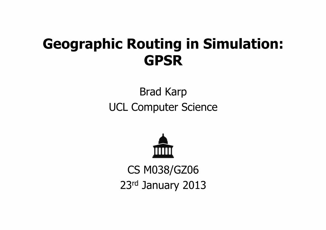
Original Motivation (2000): Rooftop Networks
• Potentially lower-cost alternative to cellular architecture (no backhaul to every base station)
6
Motivation (2010+): Sensornets
• Many sensors, widely dispersed • Sensor: radio, transducer(s), CPU,
storage, battery • Multiple wireless hops, forwarding sensor-
to-sensor to a base station What communication primitives will thousand- or million-node sensornets need?

7
“Scalability” in Sensor Networks
• Resource constraints drive metrics
• State per node: minimize • Energy consumed: minimize • Bandwidth consumed: minimize
• System scale in nodes: maximize • Operation success rate: maximize
8
Outline
• Motivation • Context • Algorithm
– Greedy forwarding – Graph planarization – Perimeter forwarding
• Evaluation in simulation • Footnotes
– Open questions – Foibles of simulation

9
The Routing Problem • Each router has unique ID • Packets stamped with
destination node ID • Router must choose next hop
for received packet • Routers communicate to
accumulate state for use in forwarding decisions
• Routes change with topology • Evaluation metrics:
– Routing protocol message cost – Data delivery success rate – Route length (hops) – Per-router state
S
D

10
The Routing Problem • Each router has unique ID • Packets stamped with
destination node ID • Router must choose next hop
for received packet • Routers communicate to
accumulate state for use in forwarding decisions
• Routes change with topology • Evaluation metrics:
– Routing protocol message cost – Data delivery success rate – Route length (hops) – Per-router state
S
D
?

11
The Routing Problem • Each router has unique ID • Packets stamped with
destination node ID • Router must choose next hop
for received packet • Routers communicate to
accumulate state for use in forwarding decisions
• Routes change with topology • Evaluation metrics:
– Routing protocol message cost – Data delivery success rate – Route length (hops) – Per-router state
S
D
12
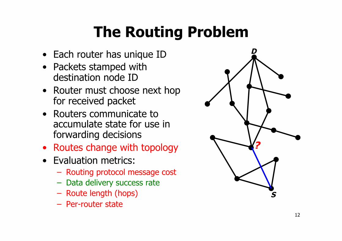
The Routing Problem • Each router has unique ID • Packets stamped with
destination node ID • Router must choose next hop
for received packet • Routers communicate to
accumulate state for use in forwarding decisions
• Routes change with topology • Evaluation metrics:
– Routing protocol message cost – Data delivery success rate – Route length (hops) – Per-router state
S
D
?
13
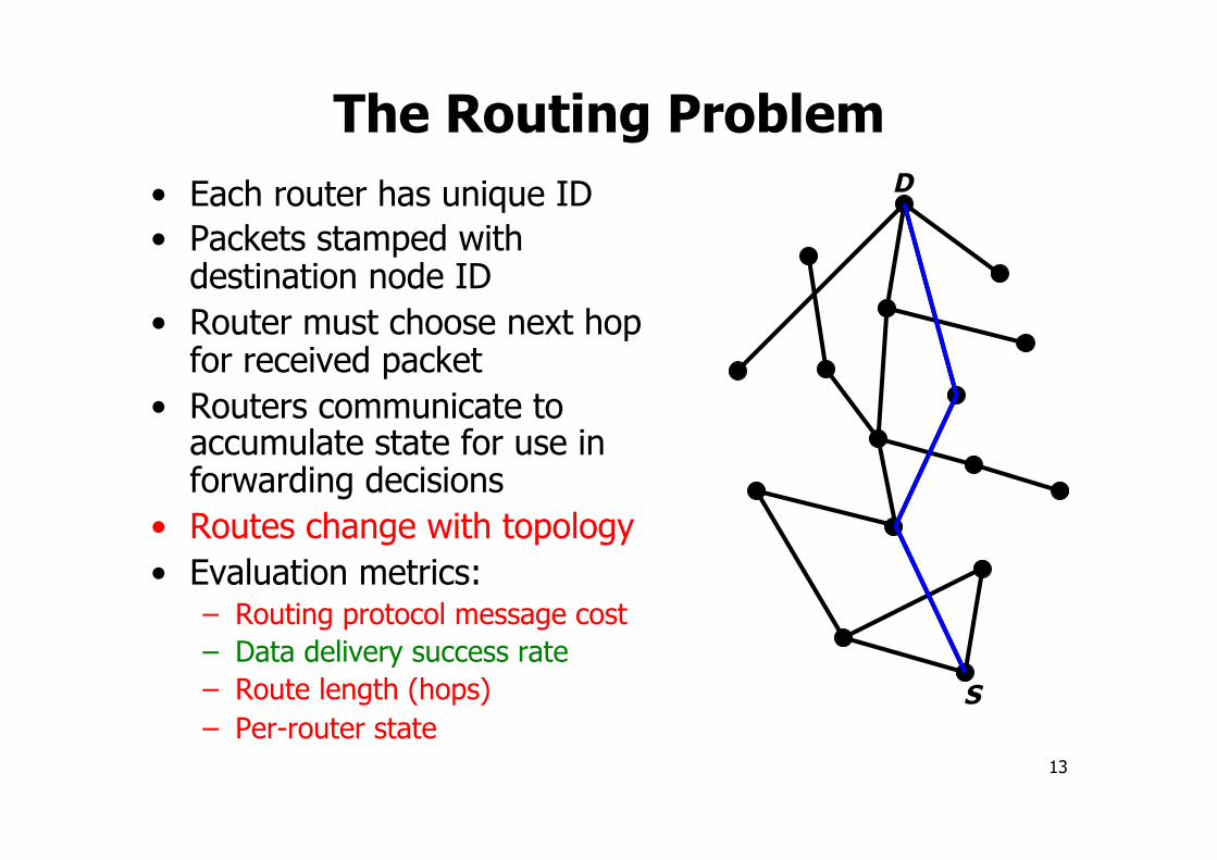
The Routing Problem • Each router has unique ID • Packets stamped with
destination node ID • Router must choose next hop
for received packet • Routers communicate to
accumulate state for use in forwarding decisions
• Routes change with topology • Evaluation metrics:
– Routing protocol message cost – Data delivery success rate – Route length (hops) – Per-router state
S
D

14
Why Are Topologies Dynamic?
• Node failure – Battery depletion – Hardware malfunction – Physical damage (harsh environment)
• Link failure – Changing RF interference sources – Mobile obstacles change multi-path fading
• Node mobility – In-range neighbor set constantly changing – Extreme case for routing scalability – Not commonly envisioned for sensor networks
15
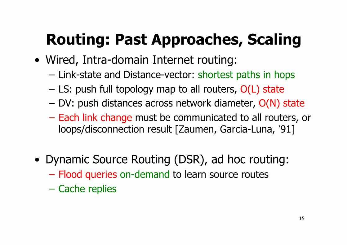
Routing: Past Approaches, Scaling • Wired, Intra-domain Internet routing:
– Link-state and Distance-vector: shortest paths in hops – LS: push full topology map to all routers, O(L) state – DV: push distances across network diameter, O(N) state – Each link change must be communicated to all routers, or
loops/disconnection result [Zaumen, Garcia-Luna, ’91]
• Dynamic Source Routing (DSR), ad hoc routing: – Flood queries on-demand to learn source routes – Cache replies
16
Scaling Routing (cont’d)
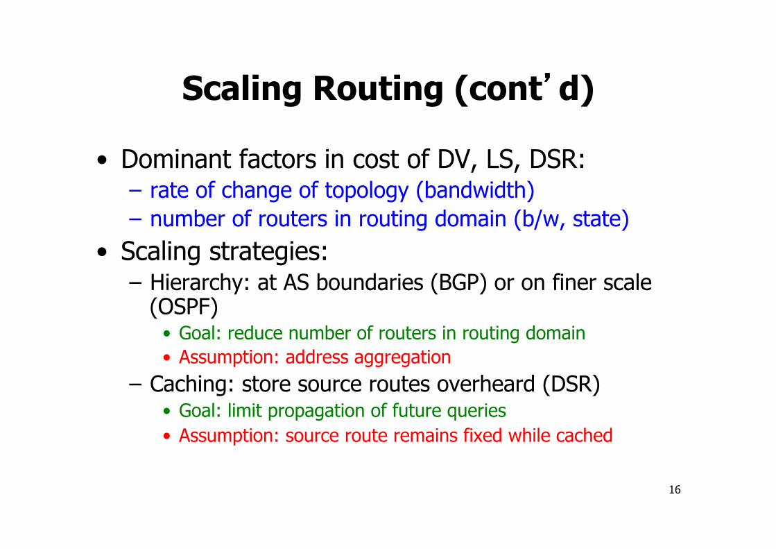
• Dominant factors in cost of DV, LS, DSR: – rate of change of topology (bandwidth) – number of routers in routing domain (b/w, state)
• Scaling strategies: – Hierarchy: at AS boundaries (BGP) or on finer scale
(OSPF) • Goal: reduce number of routers in routing domain • Assumption: address aggregation
– Caching: store source routes overheard (DSR) • Goal: limit propagation of future queries • Assumption: source route remains fixed while cached

17
Scaling Routing (cont’d)
• Dominant factors in cost of DV, LS, DSR: – rate of change of topology (bandwidth) – number of routers in routing domain (b/w, state)
• Scaling strategies: – Hierarchy: at AS boundaries (BGP) or on finer scale
(OSPF) • Goal: reduce number of routers in routing domain • Assumption: address aggregation
– Caching: store source routes overheard (DSR) • Goal: limit propagation of future queries • Assumption: source route remains fixed while cached
Today: Internet routing scales because of IP prefix aggregation; not easily applicable in sensornets Can we achieve per-node state independent of N? Can we reduce bandwidth spent communicating topology changes?

18
Central idea: Machines can know their geographic locations.
Route using geography. • Packet destination field: location of destination • Nodes all know own positions, e.g.,
– by GPS (outdoors) – by surveyed position (for non-mobile nodes) – by short-range localization (indoors, [AT&T Camb,
1997], [Priyantha et al., 2000]) – &c.
• Assume an efficient node location registration/lookup system (e.g., GLS [Li et al., 2000]) to support host-centric addressing
Greedy Perimeter Stateless Routing (GPSR)

19
Assumptions
• Bi-directional radio links (unidirectional links may be blacklisted)
• Network nodes placed roughly in a plane • Radio propagation in free space; distance
from transmitter determines signal strength at receiver
• Fixed, uniform radio transmitter power

20
Greedy Forwarding
• Nodes learn immediate neighbors’ positions from beaconing/piggybacking on data packets
• Locally optimal, greedy next hop choice: – Neighbor geographically nearest destination
D x
y

21
Greedy Forwarding
• Nodes learn immediate neighbors’ positions from beaconing/piggybacking on data packets
• Locally optimal, greedy next hop choice: – Neighbor geographically nearest destination
D x
y
Neighbor must be strictly closer to avoid loops

22
In Praise of Geography
• Self-describing • As node density increases, shortest path
tends toward Euclidean straight line between source and destination
• Node’s state concerns only one-hop neighbors: – Low per-node state: O(density) – Low routing protocol overhead: state pushed
only one hop

23
Greedy Forwarding Failure
Greedy forwarding not always possible! Consider: D
x
z v
w y

24
Greedy Forwarding Failure
Greedy forwarding not always possible! Consider: D
x
z v
void
w y

25
Greedy Forwarding Failure
Greedy forwarding not always possible! Consider: D
x
z v
void
w y
How can we circumnavigate voids? …based only on one-hop neighborhood?
26
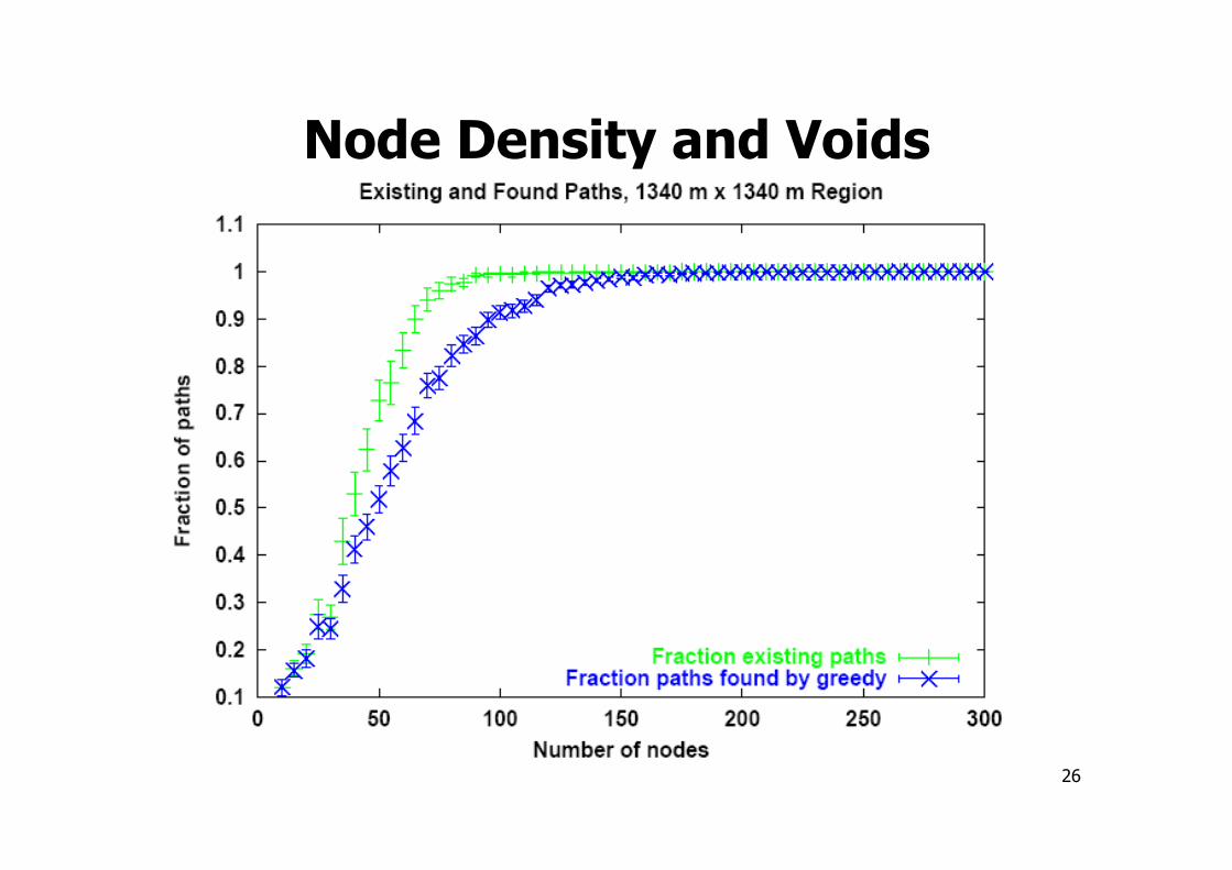
Node Density and Voids

27
Node Density and Voids
Voids more prevalent in sparser topologies

28
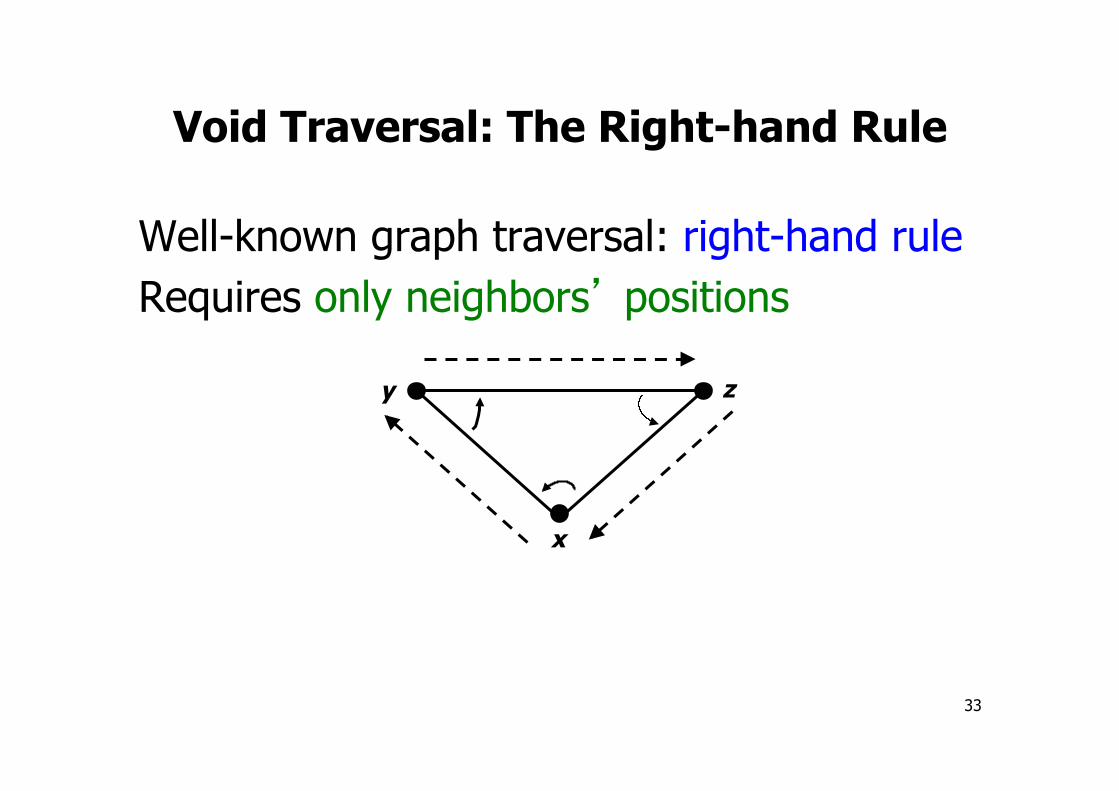
Well-known graph traversal: right-hand rule Requires only neighbors’ positions
Void Traversal: The Right-hand Rule
x
y z

29
Well-known graph traversal: right-hand rule Requires only neighbors’ positions
Void Traversal: The Right-hand Rule
x
y z

30
Well-known graph traversal: right-hand rule Requires only neighbors’ positions
Void Traversal: The Right-hand Rule
x
y z

31
Well-known graph traversal: right-hand rule Requires only neighbors’ positions
Void Traversal: The Right-hand Rule
x
y z

32
Well-known graph traversal: right-hand rule Requires only neighbors’ positions
Void Traversal: The Right-hand Rule
x
y z
33
Well-known graph traversal: right-hand rule Requires only neighbors’ positions
Void Traversal: The Right-hand Rule
x
y z

34
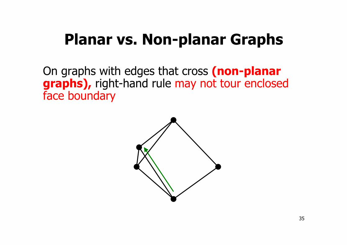
Planar vs. Non-planar Graphs
On graphs with edges that cross (non-planar graphs), right-hand rule may not tour enclosed face boundary
35
Planar vs. Non-planar Graphs
On graphs with edges that cross (non-planar graphs), right-hand rule may not tour enclosed face boundary

36
Planar vs. Non-planar Graphs
On graphs with edges that cross (non-planar graphs), right-hand rule may not tour enclosed face boundary

37
Planar vs. Non-planar Graphs
On graphs with edges that cross (non-planar graphs), right-hand rule may not tour enclosed face boundary

38
Planar vs. Non-planar Graphs
On graphs with edges that cross (non-planar graphs), right-hand rule may not tour enclosed face boundary

39
Planar vs. Non-planar Graphs
On graphs with edges that cross (non-planar graphs), right-hand rule may not tour enclosed face boundary

40
Planar vs. Non-planar Graphs
On graphs with edges that cross (non-planar graphs), right-hand rule may not tour enclosed face boundary

41
Planar vs. Non-planar Graphs
On graphs with edges that cross (non-planar graphs), right-hand rule may not tour enclosed face boundary

42
Planar vs. Non-planar Graphs
On graphs with edges that cross (non-planar graphs), right-hand rule may not tour enclosed face boundary

43
Planar vs. Non-planar Graphs
On graphs with edges that cross (non-planar graphs), right-hand rule may not tour enclosed face boundary

44
Planar vs. Non-planar Graphs
On graphs with edges that cross (non-planar graphs), right-hand rule may not tour enclosed face boundary

45
Planar vs. Non-planar Graphs
On graphs with edges that cross (non-planar graphs), right-hand rule may not tour enclosed face boundary
How to remove crossing edges without partitioning graph? And using only single-hop neighbors’ positions?
46
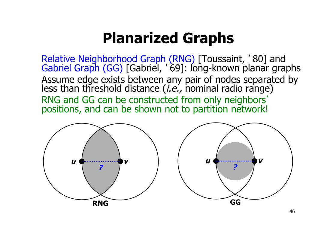
Planarized Graphs Relative Neighborhood Graph (RNG) [Toussaint, ’80] and Gabriel Graph (GG) [Gabriel, ’69]: long-known planar graphs Assume edge exists between any pair of nodes separated by less than threshold distance (i.e., nominal radio range) RNG and GG can be constructed from only neighbors’ positions, and can be shown not to partition network!
u v ?
u v ?
RNG GG

47
Planarized Graphs Relative Neighborhood Graph (RNG) [Toussaint, ’80] and Gabriel Graph (GG) [Gabriel, ’69]: long-known planar graphs Assume edge exists between any pair of nodes separated by less than threshold distance (i.e., nominal radio range) RNG and GG can be constructed from only neighbors’ positions, and can be shown not to partition network!
u v w
? u v
?
RNG GG

48
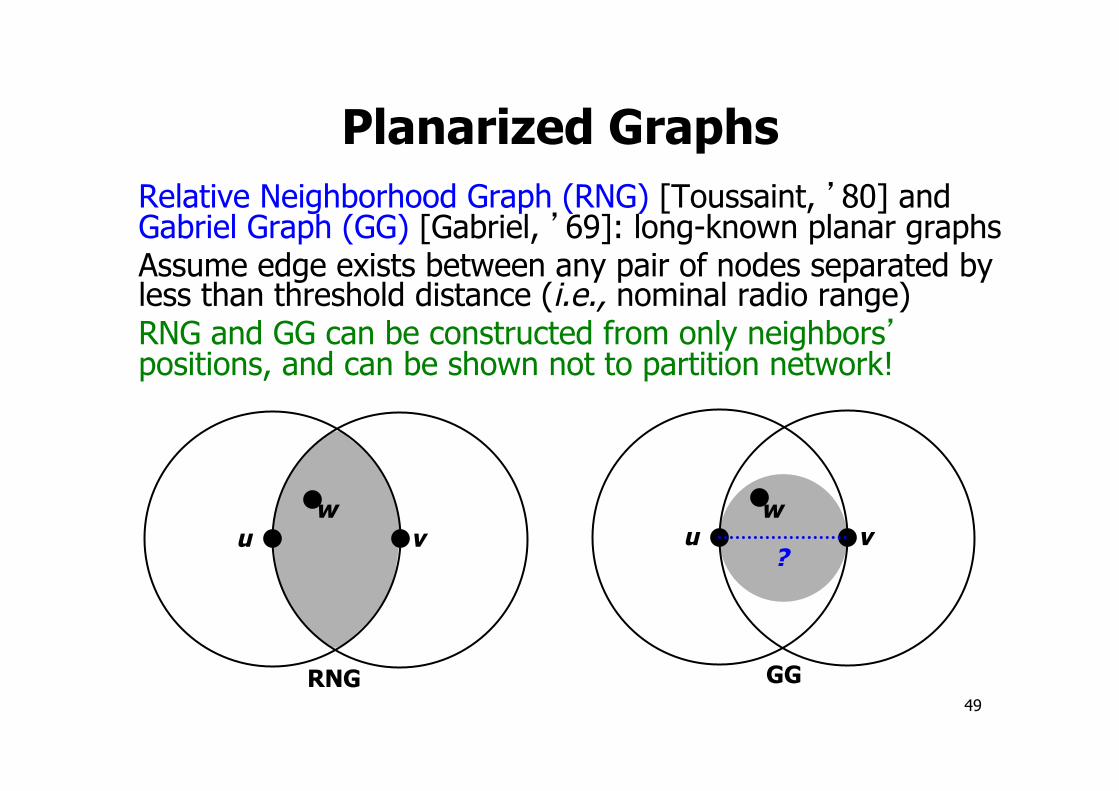
Planarized Graphs Relative Neighborhood Graph (RNG) [Toussaint, ’80] and Gabriel Graph (GG) [Gabriel, ’69]: long-known planar graphs Assume edge exists between any pair of nodes separated by less than threshold distance (i.e., nominal radio range) RNG and GG can be constructed from only neighbors’ positions, and can be shown not to partition network!
u v w
u v ?
RNG GG
49
Planarized Graphs Relative Neighborhood Graph (RNG) [Toussaint, ’80] and Gabriel Graph (GG) [Gabriel, ’69]: long-known planar graphs Assume edge exists between any pair of nodes separated by less than threshold distance (i.e., nominal radio range) RNG and GG can be constructed from only neighbors’ positions, and can be shown not to partition network!
u v w
u v w
?
RNG GG

50
Planarized Graphs Relative Neighborhood Graph (RNG) [Toussaint, ’80] and Gabriel Graph (GG) [Gabriel, ’69]: long-known planar graphs Assume edge exists between any pair of nodes separated by less than threshold distance (i.e., nominal radio range) RNG and GG can be constructed from only neighbors’ positions, and can be shown not to partition network!
u v w
u v w
RNG GG

51
Planarized Graphs Relative Neighborhood Graph (RNG) [Toussaint, ’80] and Gabriel Graph (GG) [Gabriel, ’69]: long-known planar graphs Assume edge exists between any pair of nodes separated by less than threshold distance (i.e., nominal radio range) RNG and GG can be constructed from only neighbors’ positions, and can be shown not to partition network!
u v w
u v w
RNG GG
Euclidean MST (so connected) RNG GG
Delaunay Triangulation (so planar) ⊆ ⊆
⊆

52
Planarized Graphs: Example
200 nodes, placed uniformly at random on 2000-by-2000-meter region; 250-meter radio range
Full Graph GG Subgraph RNG Subgraph

53
Full Greedy Perimeter Stateless Routing
• All packets begin in greedy mode • Greedy mode uses full graph • Upon greedy failure, node marks its location in
packet, marks packet in perimeter mode • Perimeter mode packets follow simple planar
graph traversal: – Forward along successively closer faces by right-hand
rule, until reaching destination – Packets return to greedy mode upon reaching node
closer to destination than perimeter mode entry point

54
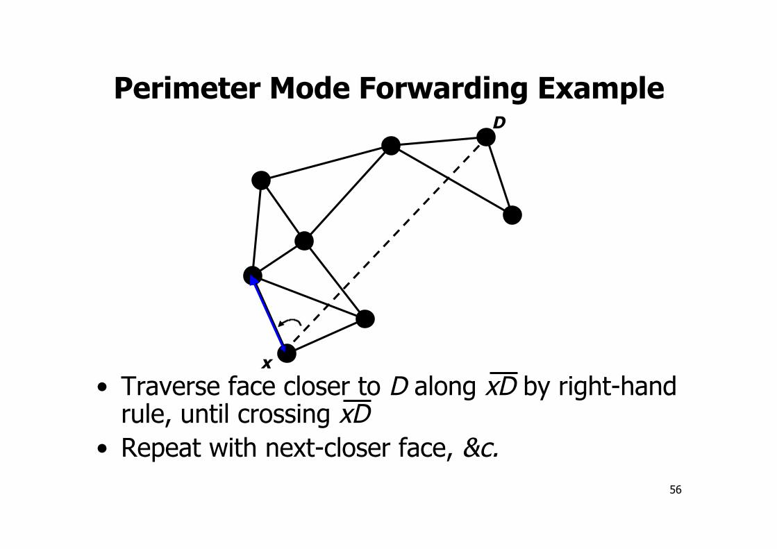
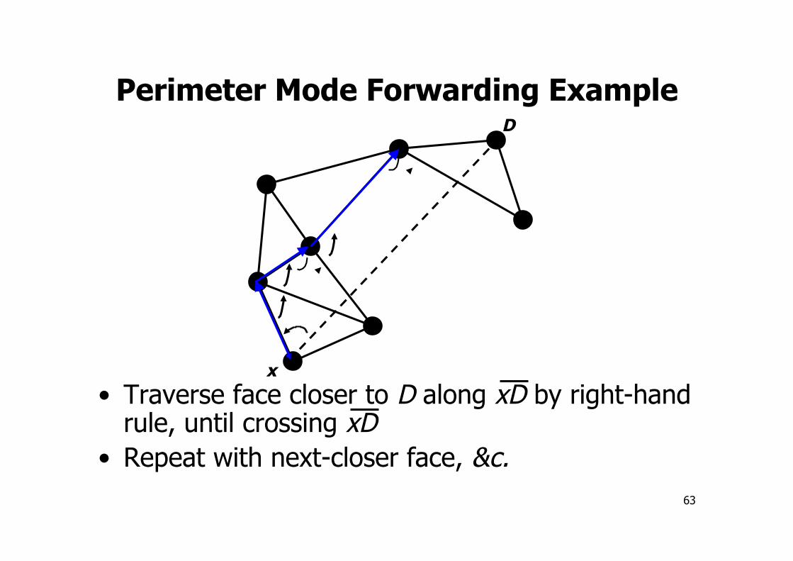
Perimeter Mode Forwarding Example
• Traverse face closer to D along xD by right-hand rule, until crossing xD
• Repeat with next-closer face, &c.
x
D

55
Perimeter Mode Forwarding Example
• Traverse face closer to D along xD by right-hand rule, until crossing xD
• Repeat with next-closer face, &c.
x
D
56
Perimeter Mode Forwarding Example
• Traverse face closer to D along xD by right-hand rule, until crossing xD
• Repeat with next-closer face, &c.
x
D

57
Perimeter Mode Forwarding Example
• Traverse face closer to D along xD by right-hand rule, until crossing xD
• Repeat with next-closer face, &c.
x
D
58
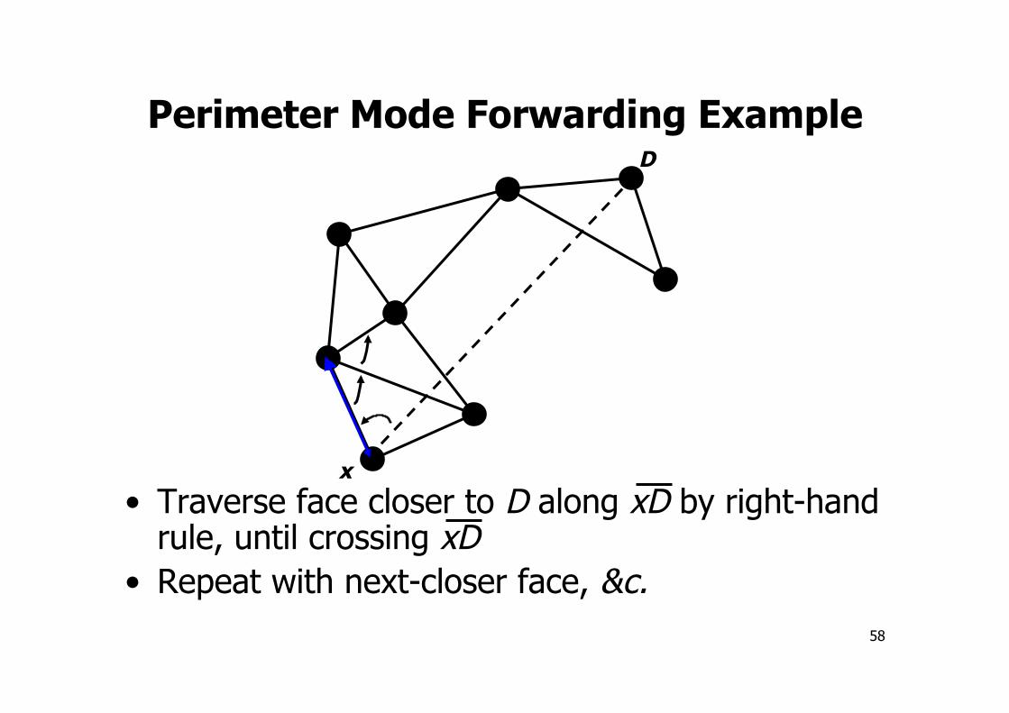
Perimeter Mode Forwarding Example
• Traverse face closer to D along xD by right-hand rule, until crossing xD
• Repeat with next-closer face, &c.
x
D

59
Perimeter Mode Forwarding Example
• Traverse face closer to D along xD by right-hand rule, until crossing xD
• Repeat with next-closer face, &c.
x
D

60
Perimeter Mode Forwarding Example
• Traverse face closer to D along xD by right-hand rule, until crossing xD
• Repeat with next-closer face, &c.
x
D

61
Perimeter Mode Forwarding Example
• Traverse face closer to D along xD by right-hand rule, until crossing xD
• Repeat with next-closer face, &c.
x
D

62
Perimeter Mode Forwarding Example
• Traverse face closer to D along xD by right-hand rule, until crossing xD
• Repeat with next-closer face, &c.
x
D
63
Perimeter Mode Forwarding Example
• Traverse face closer to D along xD by right-hand rule, until crossing xD
• Repeat with next-closer face, &c.
x
D

64
Perimeter Mode Forwarding Example
• Traverse face closer to D along xD by right-hand rule, until crossing xD
• Repeat with next-closer face, &c.
x
D

65
Perimeter Mode Forwarding Example
• Traverse face closer to D along xD by right-hand rule, until crossing xD
• Repeat with next-closer face, &c.
x
D

66
Protocol Tricks for Dynamic Networks
• Use of MAC-layer failure feedback: As in DSR [Broch, Johnson, ’98], interpret retransmit failure reports from 802.11 MAC as indication neighbor gone out-of-range
• Interface queue traversal and packet purging: Upon MAC retransmit failure for a neighbor, remove packets to that neighbor from IFQ to avoid head-of-line blocking of 802.11 transmitter during retries
• Promiscuous network interface: Reduce beacon load and keep positions stored in neighbor tables current by tagging all packets with forwarding node’s position
• Planarization triggers: Re-planarize upon acquisition of new neighbor and every loss of former neighbor, to keep planarization up-to-date as topology changes
67
Outline
• Motivation • Context • Algorithm
– Greedy forwarding – Graph planarization – Perimeter forwarding
• Evaluation in simulation • Footnotes
– Open questions – Foibles of simulation

68
Evaluation: Simulations
• ns-2 with wireless extensions [Broch et al., ’98]; full 802.11 MAC, free space physical propagation
• Topologies:
• 30 2-Kbps CBR flows; 64-byte data packets • Random Waypoint Mobility in [1, 20 m/s]; Pause
Time [0, 30, 60, 120s]; 1.5s GPSR beacons
Nodes Region Density
50 1500 m x 300 m 1 node / 9000 m2
200 3000 m x 600 m 1 node / 9000 m2
50 1340 m x 1340 m 1 node / 35912 m2

69
Packet Delivery Success Rate (50, 200; Dense)
70
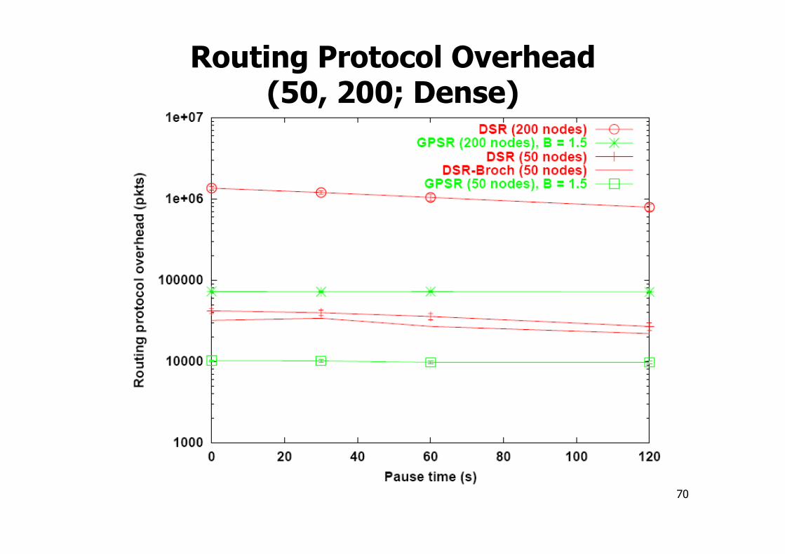
Routing Protocol Overhead (50, 200; Dense)

71
Path Length (50; Dense)
72
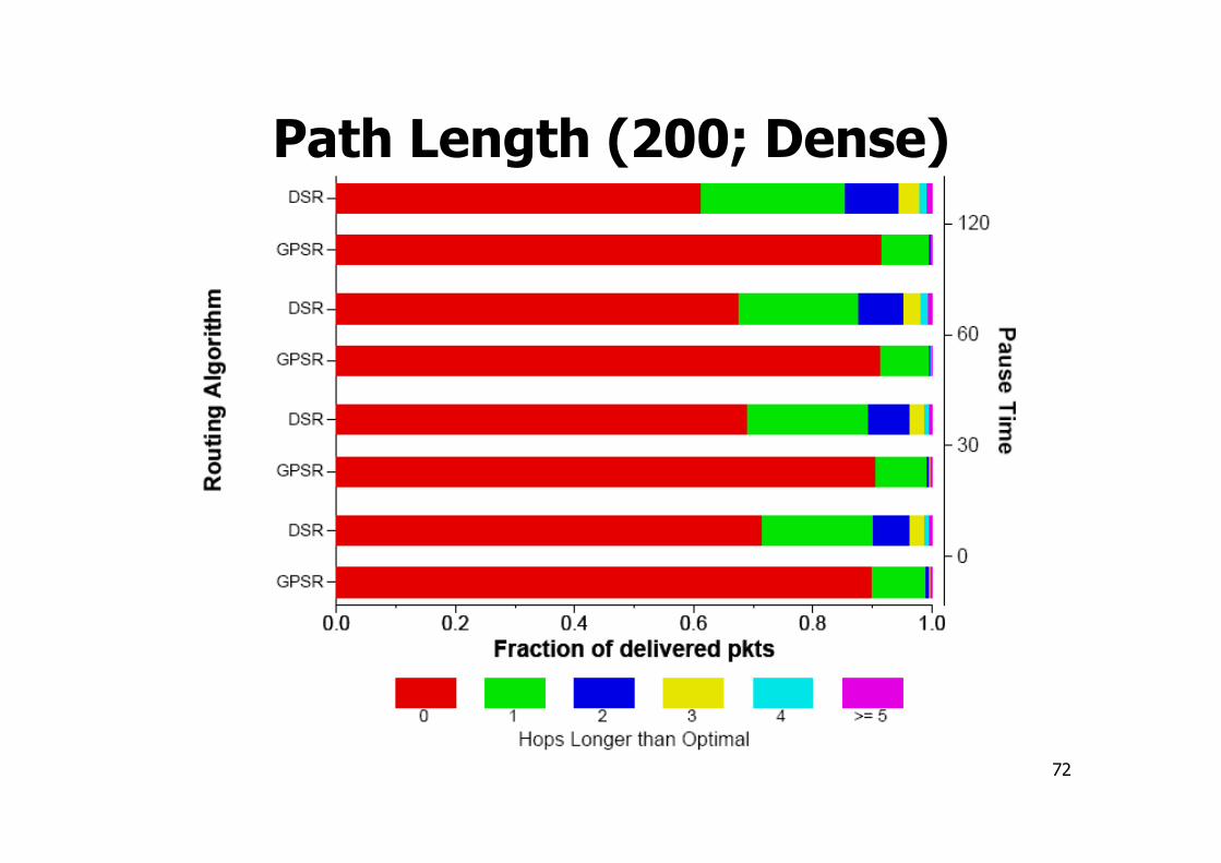
Path Length (200; Dense)
73
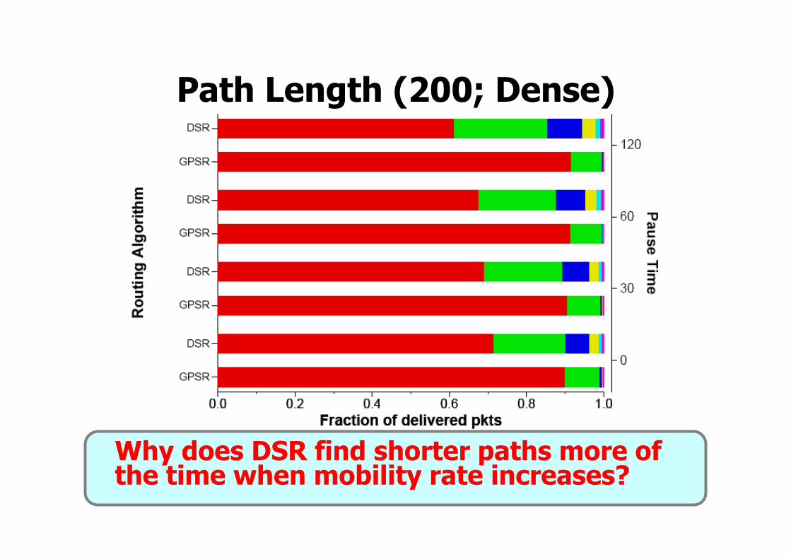
Path Length (200; Dense)
Why does DSR find shorter paths more of the time when mobility rate increases?

74
State Size (200; Dense)
75
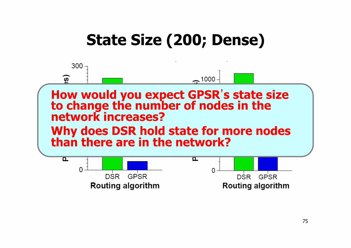
State Size (200; Dense)
How would you expect GPSR’s state size to change the number of nodes in the network increases? Why does DSR hold state for more nodes than there are in the network?

76
Critical Thinking
• Based on the results thus far (indeed, all results in the paper), what do we know about the performance of GPSR’s perimeter mode? – Would you expect it to be more or less
reliable than greedy mode? – Would you expect use of perimeter mode to
affect path length?

77
Critical Thinking
• Based on the results thus far (indeed, all results in the paper), what do we know about the performance of GPSR’s perimeter mode? – Would you expect it to be more or less
reliable than greedy mode? – Would you expect use of perimeter mode to
affect path length?
Evaluation in paper reveals nearly nothing about performance of perimeter mode! Why doesn’t it?
78
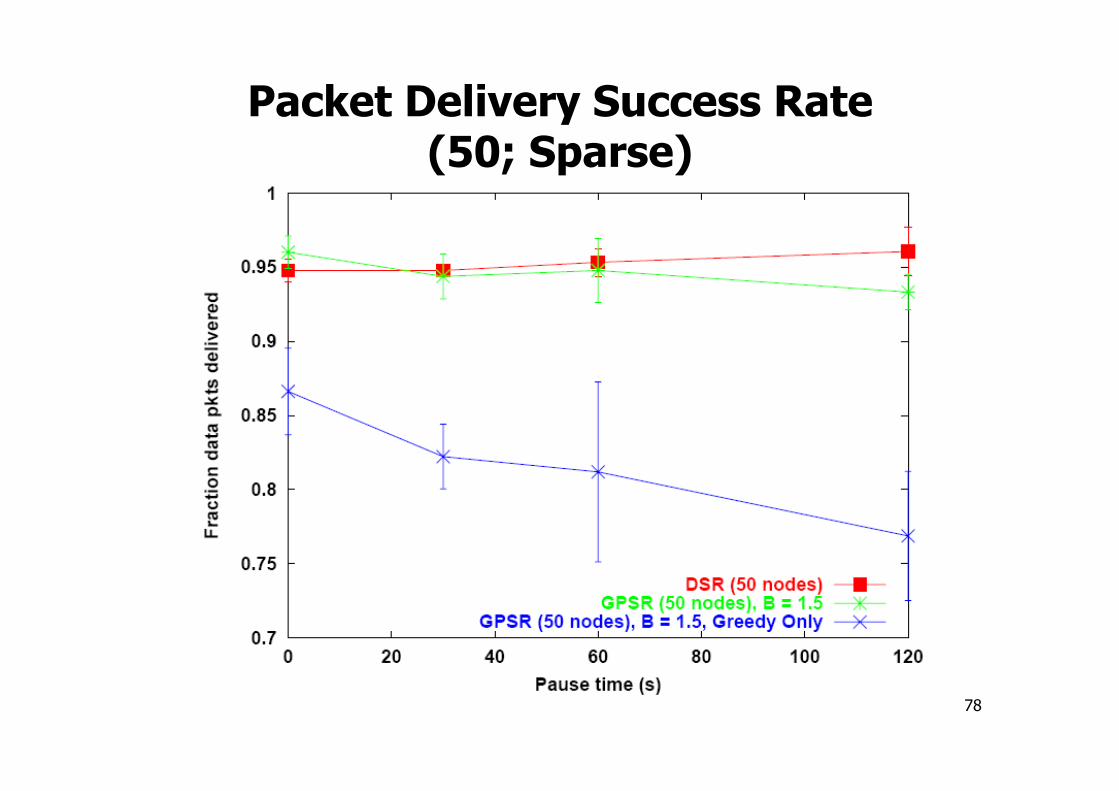
Packet Delivery Success Rate (50; Sparse)
79
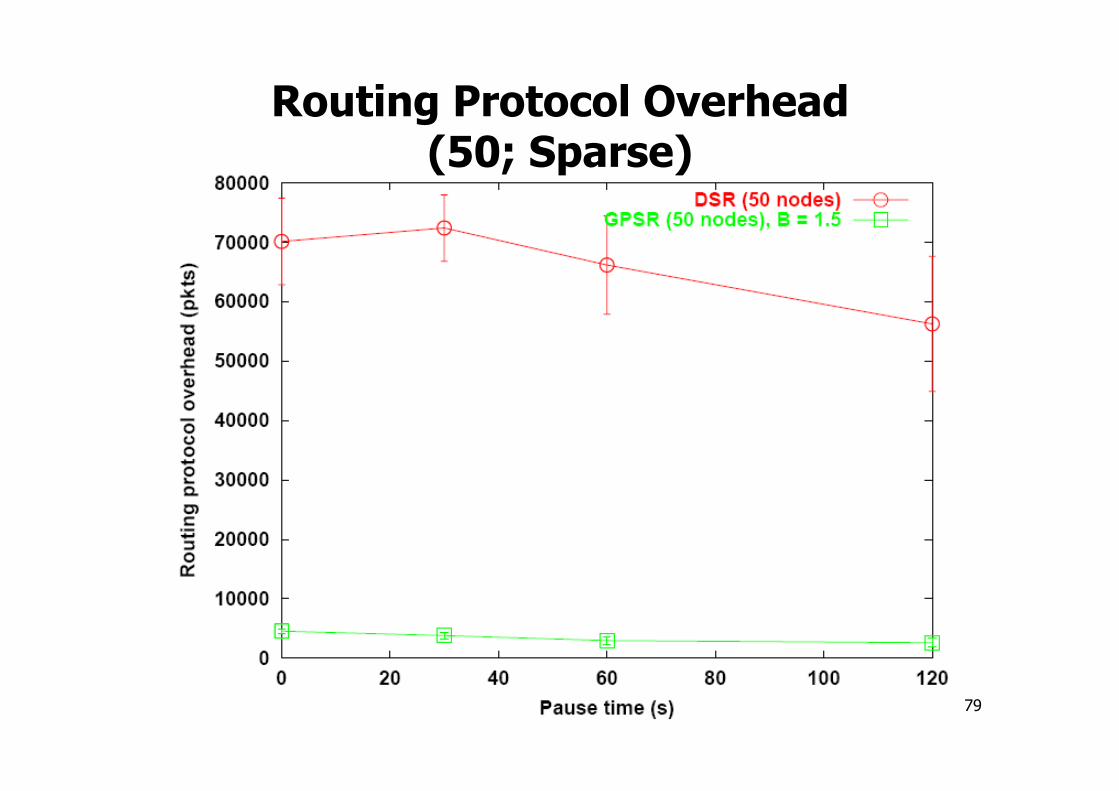
Routing Protocol Overhead (50; Sparse)

80
Path Length (50; Sparse)

81
Outline
• Motivation • Context • Algorithm
– Greedy forwarding – Graph planarization – Perimeter forwarding
• Evaluation in simulation • Footnotes
– Open questions – Foibles of simulation
82
Open Questions
• How to route geographically in 3D? – Greedy mode? – Perimeter mode? – More in CLDP paper (next)…
• Effect of radio-opaque obstacles? – More in CLDP paper (next) …
• Effect of position errors? – More in CLDP paper (next) … J
• “Better” planar graphs than GG, RNG? – See [Guibas et al., 2001]
• Name-to-location database, built atop geo routing? – See [GLS, Li et al., MobiCom 2000]
83
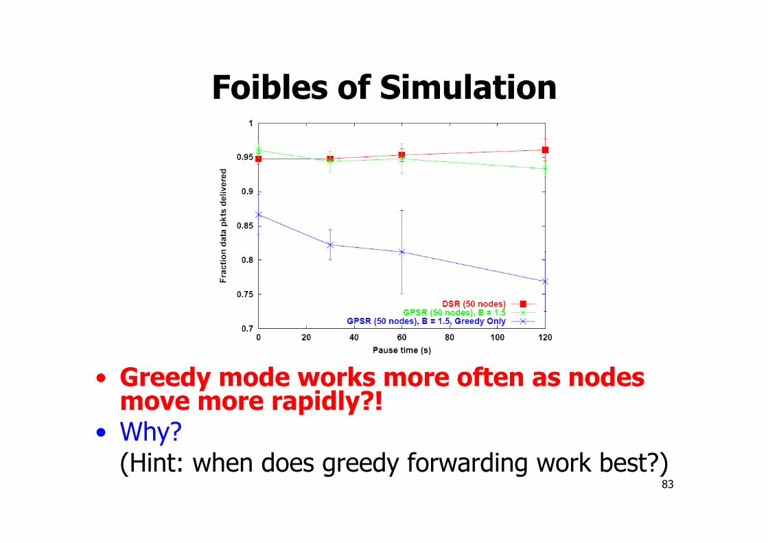
Foibles of Simulation
• Greedy mode works more often as nodes move more rapidly?!
• Why? (Hint: when does greedy forwarding work best?)

84
Recap: Scalability via Geography with GPSR
Key scalability properties: • Small state per router: O(D), not O(N) or O(L)
as for shortest-path routing, where D = density (neighbors), N = total nodes, L = total links
• Low routing protocol overhead: each node merely single-hop broadcasts own position periodically
• Approximates shortest paths on dense networks • Delivers more packets successfully on dynamic
topologies than shortest-paths routing protocols