Computers & Coeosciences Vol. g, No. 1, pp. 61-68, 1982 00N-~04nl2J01O051-0~03.0010 Printed in Great Britain. ~ I n Perpmou Press Ltd.

GEOMAN: A FORTRAN PROGRAM FOR THE MANAGEMENT OF GEOLOGICAL THIN SECTION DATA

ERIC DAVAUD and ANDRE STRASSER Ecole des Sciences de la Terre, University of Geneva, 13 Rue des Maraichers, CH-1211 Geneva, Switzerland

(Received 5 .lanuary 1981; revised 21 June 1981)

Abm'act--A program for treating large numbers of qualitative and/or quantitative geological thin section data has been developed. Data are coded, stored in a direct access data bank, and extracted selectively for treatmenL The system is easy to handle and flexible, that is the user can choose descriptive attn'butes (variables) and select parameters for different computational operations. The codification and program can be applied to all rock types. The treatment includes: Loading of data bank, Updating of data bank, Selection of samples and variables, Edition of samples, Variable distribution in geological sections, Histograms, Scatter diagrams, Association analysis and Correspondence analysis.

Key Words: Classification, Data processing, Paleontology, Sedimentology, Stratigraphy.

INTRODUCTION The classical method of studying geological thin sections is to fill out checklists, make notes on pieces of paper or simply remember what the thin sections look like. However, working with large amounts of data and often complex relationships between rock components is cumbersome. Information is lost, and trends or regulari- ties in the studied sequences are not detected. Further- more, looking for a specific item in the mass of data requires considerable time. Here, the use of a computer is helpful; data can be stored permanently, extracted selectively and treated. In addition, statistical programs help to evaluate the data.

In 1976, Charollais and Davand published a computer program for the treatment and analysis of sedimentary microfacies. Experiences collected during the use of this program (Strasser, 1979) and discussions with coilegues led to a new concept and to the development of GEOMAN.

Flexibility was one important requirement. Because the user now can choose his own variable codenames, not only sedimentary rock thin sections, but almost any set of multivariate qualitative and or quantitative data can be treated. A detailed description of the samples is possible. Also, coding rules are simple and easy to memorize. Another new feature is the direct access data bank. This system permits fast extraction of selected samples. The data bank can be extended and modified.

The statistical and descriptive subprograms, treating extracted data represent only a selection of possible routines. It is up to the user to add new subprograms, or to modify existing ones to meet his demands.

CODIFICATION

For computer treatment, information contained in the samples has to be coded. The coded sample must encompass as much original information as possible, taking into account complex geometrical and genetic interrelations between rock components (variables). However, codification should be easy to perform, and data have to be suitable for further treatment.

Each sample is identified by a sample number (4

alphanumeric characters), coordinates (optional), posi- tion in geological section and range in the section. Vari- ables are descnl~ed by 4-character mnemonic codes (let- ters or digits). The user is free to choose his own codenames; not only microscopic rock components, but also macroscopic features, and geographic and strati- graphic information may be considered as variables. Before coding the samples, it is useful to establish a variable list, including a 2~haracter desc~riptiou of the codenames. Emphasis can be placed by introducing different codenames for different populations or genera- tions of one component.

Example: JURA URGO XBED WACK QURZ CEM1 CEM2

JURA MOUNTAINS UROONIAN CROSS-BEDDING WACKESTONE (DUNHAM CLASS.) DEFRITAL QUARTZ FIRST GENERATION CEMENT SECOND GENERATION CEMENT.

This variable list also can be used as a checklist. Fur- thermore, it can be modified by adding or changing codenames at any time. The frequency of a variable is indicated by one or two digits after a slash, its diameter by one to four digits after a comma.

In parenthesis, up to 5 variables can be added to describe chronological or geometrical relationships be- tween two or more rock components, or to give a detailed description of a rock component. Each of the second-order variables may be specified further by a frequency number and by one third-order variable, also in parenthesis. For example, INTR(ORAN OOID(QURZ)) describes an INTRaclast composed of a GRAiNstone containing OOIDs with QUsRtZ grains as nuclei.

Up to a total of 360 characters can be used to describe one sample.

Figure 1 shows possible codifications of three sedi- mentary rock thin sections. A simple relationship be- tween components and matrix is represented in Figure

61

62 ERIC DAVAUD and ANDRE STRASSER

, ~ : : ~ . :~i!:::i~:?:. :~:'

5OOU

~cg MICR/80 8ICL/20,120 FOPS(TEXT)

GleN CEm SPAR(CrMZ)

b Pru. OOZO(BXCL) INTR(ROUN PELL/60 OOIO/lO(NICR) NICR/30) LAME(BORE RECR)

soo~

WACK MICR/80 QURZ/20,50 C ~HARD(PHOS BORE EROO)

GRAN SPAR/S0 PELLIZO,200 ECHI/20,220 I./~E/10o200

5oo/4

Figure 1. Codification of sedimentary rock thin sections (see text for comments).

l(a): it is a WACKestone (Dunham classification) with 80 percent of the thin section area consisting of MICRite, and 20 percent of BIoCLasts with a mean diameter of 120 microns (units defined by user). Some FORAminifera are identified as TEXTularids.

The rock components of the GRAiNstone in Figure l(b) have more complicated geometrical and genetic in- terrelations; a first generation cement (CEMI) rims the grains. SPARite filling the pores is a second generation cement (CEM2). The OOIDs contain BIoCLasts as a core. ROUNded INTRaclasts consist of PELLets (60 percent of the intraclast), MICRitic OOIDs (10 percent of the intraclast) and of MICRite (30 percent of the intraclast). Also present are BOREd and RECRystallized LAMEllibranch fragements. In this example (Fig. lb), a subordinate variable can describe either the geometry (ROUN), the time relationship (CEM2), the composition (MICR), or a combination of the three (BICL as core of OOID). However, note that MICR represents MICRite as well as MICRitic. It is up to the user to specify clearly the differences by introducing two codenames.

Figure l(c) shows different types of microfacies in the same thin section, a WACKestone with MICRite and detrial QUaRtZ, a PHOSphoritic, BOREd, and ERODed HARDground, and a GRAiNstone with SPARite, PELLets, ECHinoderms, and LAMEllihranchs. To avoid distortion of the original information, these three micro- facies will have to be coded separately.

It is outside the scope of this paper to deal with the problems and techniques of estimating frequencies and grainsize in a thin section, or identifying the various rock components (Schoile, 1978, 1979; F10gel, 1978). How accurately the thin section is described and how many details are codified will depend on the analysis to be performed.

PltOGPJLM 5'I~UC'I'URE AND DATA TliEATI~gNT

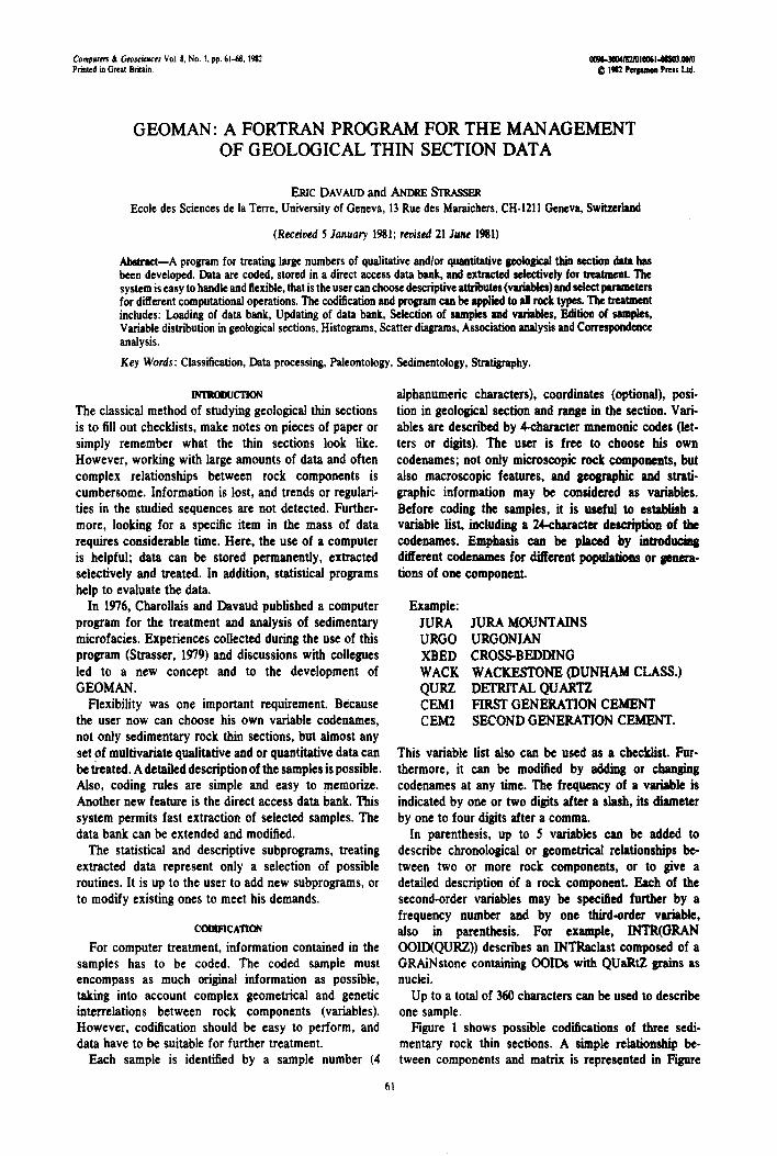
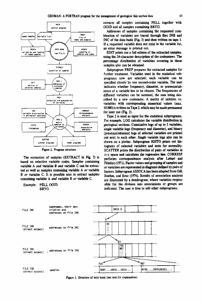
The program concept is summarized in Figure 2 and the data flow indicated by arrows. MAIN is the control program, which reads instructions and calls the cor- responding subprograms.

The first operation is the creation of a data bank. The variable list (codenames and description) is introduced directly into the data bank. The coded data are read and validated by INDATA. If coding errors are detected or a variable code does not exist in the variable list, the sample is rejected. This prevents incorrect data from entering the data bank.

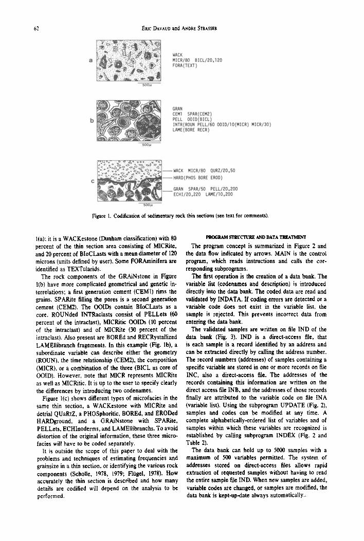
The validated samples are written on file IND of the data bank (Fig. 3). IND is a direct-access file, that is each sample is a record identified by an address and can be extracted directly by calling the address number. The record numbers (addresses) of samples containing a specific variable are stored in one or more records on file INC, also a direct-access file. The addresses of the records containing this information are written on the direct access file INB, and the addresses of those records finally are attributed to the variable code on file INA (variable list). Using the subprogram UPDATE (Fig. 2), samples and codes can be modified at any time. A complete alphabetically-ordered list of variables and of samples within which these variables are recognized is established by calling subprogram INDEX (Fig. 2 and Table 2).

The data bank can hold up to 5000 samples with a maximum of 500 variables permitted. The system of addresses stored on direct-access files allows rapid extraction of requested samples without having to read the entire sample file IND. When new samples are added, variable codes are changed, or samples are modified, the data bank is kept-up-date always automatically..

GEOMAN: A FORTRAN program for the management of geological thin section data

I NAIH control program

selection of samples

EDIT @ edition of

selected samples

J PREP

vlrtable distribution in 9eological sections

HISTO his~.ograms

SCATTER ] . . . . . . . scitter dtagrNIS ,, / other progrlms

Figure 2. Prolp~m structure.

INDEX 1

UPDATE updattBg of

samples and codes

CORRESP co~*r~spondence

ASSOCA ;ISSOClitiOfl Jnalysts

The extraction of samples (EXTRACT in Fig. 2) is based on selective variable codes. Samples containing variable A and variable B and variable C can be extrac- ted as well as samples containing variable A or variable B or variable C. It is possible also to extract samples containin~ variable A and variable B or variable C.

Example: PELL OOID BRYO

63

extracts all samples containing PELL together with OOID and all samples containing BRYO.

Addresses of samples containing the requested com- bination of variables are traced through files INB and INC of the data bank (Fig. 3) and then written on tape 1. If a requested variable does not exist in the variable list, an error message is printed out.

EDIT prints out a full edition of the extracted samples, using the 24-character description of the codenames. The percentage distribution of variables occuring in these samples also can be obtained.

.Subprogram PREP prepares the extracted samples for further treatment. Variables used in the statistical sub- programs now are selected; each variable can be specified closely by one second-order variable. The user indicates whether frequency, diameter, or presence/ab- sence of a variable has to be chosen. The frequencies of ditferent variables can be summed, the sum being des- cribed by a new codename. A matrix of samples vs. variables with corresponding numerical values (max. 10 000) is written on Tape 2, which may be made permanent for later use {Fig. 2).

Tape 2 is used as input for the statistical subprograms. For example, LOG calculates the variable distn'oution in geological sections. Cumulative logs of up to 5 variables, single variable logs (frequency and diameter), and binary (presence/absence) logs of selected variables are printed out next to each other. Single variable logs also can be drawn on a plotter. Subprogram HISTO prints out his- tograms of selected variables and tests for normxlity. SCATI'ER prints the distribution of pairs of variables in x-y space and calculates the regression line. CORRESP performs correspondence analysis after Lebart and Fenelon ( 1971 ). Factor values and grouping of samples and or variables are represented in diagrams defined by pairs of factors. Subprogram ASSOCA has been adapted from Gill, Boehm, and Erez (1976). Results of association analysis are illustrated by a dendrogram, where variables respon- sible for the division into associations or groups are indicated. The user is free to add other subprograms.

FILE INA

FILE INB (direct access)

FILE INC (direct access)

codenames, their des- cription and addresses on f i l e INB

addresses on f i l e INC

• addresses on f i l e IND

FILE IND (direct access) samples

IIZ I

I 705~~~~-~

. . °

. o .

. ° .

iilJ,-, .... .... .... J

Figure 3. Structure of data bank (see text for explanation).

64 ERIC DAVUD ~ffid ANDRE STRASSER

EX/cMPLE

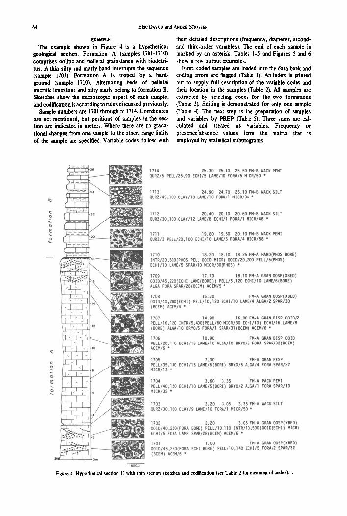
The example shown in Figure 4 is a hypothetical geological section. Formation A (samples 1701-1710) comprises oolitic and pelletal grainstones with biodetri- tus. A thin silty and marly band interrupts the sequence (sample 1703). Formation A is topped by a hard- ground (sample 1710). Alternating beds of pelletai micritic limestone and silty marls belong to formation B. Sketches show the microscopic aspect of each sample, and codification is according to rules discussed previously.

Sample numbers are 1701 through to 1714. Coordinates are not mentioned, but positions of samples in the sec- tion are indicated in meters. Where there are no grada- tional changes from one sample to the other, range limits of the sample are specified. Variable codes follow with

their detailed descriptions (frequency, diameter, second-

and third-order variables). The end of each sample is marked by an asterisk. Tables 1-5 and Figures 5 and 6 show a few output examples.

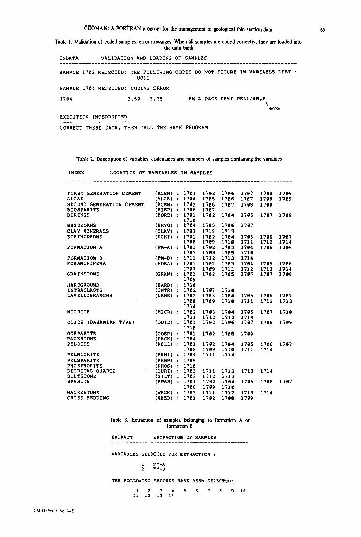
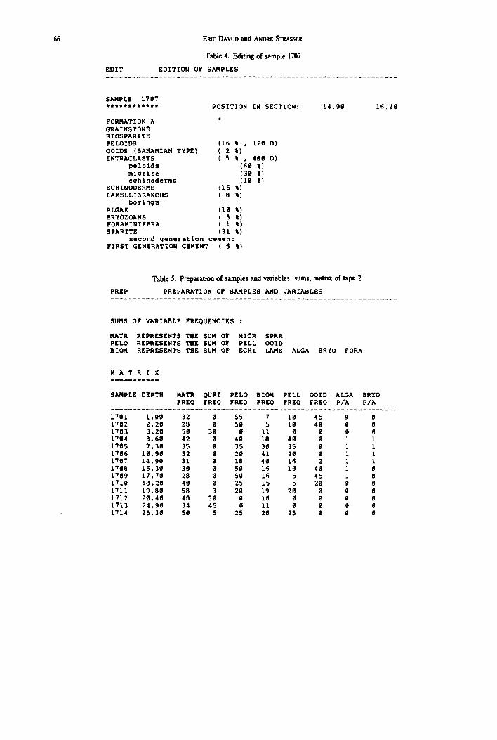
First, coded samples are loaded into the data bank and coding errors are flagged (Table 1). An index is printed out to supply full description of the variable codes and their location in the samples (Table 2). All samples are extracted by selecting codes for the two formations (Table 3). Editing is demonstrated for only one sample (Table 4). The next step is the preparation of samples and variables by PREP (Table 5). Three sums are cal- culated and treated as variables. Frequency or presence/absence values form the matrix that is employed by statistical subprograms.

t~

o

e... o

0

0

1714 Z5.30 26.10 ZS.SO FN-B MACK PEMI QURZ/5 PELL/25,90 ECHI/5 L.AgE/IO FORAI5 MICR/50 *

1713 24.90 24.70 25.10 Fg-B MACK SILT QURZ/45,100 CLAY/IO LAgE/IO FORA/1MICR/34 *

171Z 20.40 20.10 20.60 F/~B MACK SILT QURZ/30.100 CLAY/12 LANE/8 ECHI/1FORA/1MICRI48 *

1711 19.80 19.50 20.10 FM-B MACK PENI QURZ/3 PELL/ZO,IO0 ECH[/IO LAgE/5 FORA/4 HICR/S8 *

1710 18.20 18.10 18.25 FM-A HARD(PHOS BORE) !NTR/ZO,5OO(PHOS PELL OOIO N|CR) OOIO/ZO,ZO0 PELL/S(PHOS) ECHI/IO LAgE/5 SPAR/IO HICR/30(PHOS) *

1709 17.70 18.10 leg..A 6RAN OOSP(XBED) OOIO/45,220(ECHI I.AgE(BORE)) PELL/5,120 ECH[/IO LAME/8(BORE) ALGA FORA SPAR/Ze(UCEg) ACEglS *

1708 16.30 FN-A GRAN OOSP(XBED) OOIO/40,ZOO(ECH[) PELL/lO,120 ECHI/IO LAgE/4 ALGA/2 SPAR/30 (eCEM) ACE~/A *

1707 14.90 16.00 Fg-A GRAN BISP 0010/2 PELL/16,1ZO INTR/S,400(PELL/60 NICR/30 ECHI/IO) ECHI/16 LAg[/8 (BORE) ALGA/IO BRYO/S FORA/1 SPAR/31(BCEN) AC~/6 *

1706 10.90 FM-A GRAN else 0010 CELL/20,110 ECHI/15 I.AgE/IO ALGA/IO BRYO/6 FORA SPAR/32(BCEg) ACEN/6 *

1705 7.30 FN-A GRAN PESP PELL/35,130 ECHI/15 LANE/6(BORE) BRYO/S ALGA/4 FORA SPAR/22 MICRI13 *

1704 3.60 3.35 FN-A PACK PEMI PELL/40,120 ECHI/IO LAME/S(BORE) BRYO/Z ALGA/1 FORA SPAR/IO MICR/3Z *

1703 3.20 3 .05 3.35 FN-A WACK SILT OURZ/30,100 CLAY/9 LANE/IO FORA/1MICR/SO *

1702 2.20 3.05 FM-A GRAN OOSP(XBED) OOIO/40,Z20(FORA BORE) PELL/lO,110 INTR/IO,5OO(OOIO(ECHI) MICR) ECHI/5 FORA LAN~ SPAR/28(BCEM) ACEM/6 *

1701 1.00 FN-A GRAN OOSP(XBED) OOID/4S,2SO(FORA ECH! BORE) PELL/10,140 ECHI/5 FORA/2 SPAR/32 (BCEM) ACEM/6 *

Figure 4. Hypothetical section 17 with thin section sketches and codification (see Table 2 for meaning of codes). ,

OEOMAN: A FORTRAN program for the management of geological thin section data

Table 1. Validation of coded samples, error messages. When all samples are coded correctly, they are loaded into the data bank

INDATA VALIDATION AND LOADING OF SAMPLES ..........................................................................

SAMPLE 1702 REJECTED: THE FOLLOWING CODES DO NOT FIGURE IN VARIABLE LIST : OOLI

SAMPLE 1704 REJECTED: CODING ERROR

1704 3.60 3.35

EXECUTION INTERRUPTED .....................

FM-A PACK PEMI PELL/40,F

e r r o r

CORRECT THESE DATA, THEN CALL THE SAME PROGRAM

65

Table 2. Description of variables, codenames and numbers of samples containing the variables

INDEX LOCATION OF VARIABLES IN SAMPLES

FIRST GENERATION CEMENT ALGAE SECOND GENERATION CEMENT BIOSPARITE BORINGS

SRYOZOANS CLAY MINERALS ECHINODERMS

FORMATION A

FORMATION B FORAMINIFERA

GRAINSTONE

HARDGROUND INTRACLASTS LAMELLIBRANCHS

MICRITE

OOIDS (BAHAMIAN TYPE)

OOSPARITE PACKSTONE PELOIDS

PELMICRITE PELSPARITE PHOSPHORITE DETRITAL QUARTZ SILTSTONE SPARITE

WACKESTONE CROSS-BEDDING

(ACEM) : 1701 17%2 17%6 1707 1708 1709 (ALGA) : 1704 1705 17%6 17%7 17%8 1709 (BCEM) : 1702 17%6 1707 17%8 17%9 (BISP) : 17%6 1707 (BORE) : 17gl 1702 17%4 17%5 1707 17%9

1710 (BRYO) : 17%4 17%5 17%6 1707 (CLAY) : 1703 1712 1713 (ECHI) : 17%1 1702 17%4 17%5 17%6 i7%7

17%8 17%9 1710 1711 1712 1714 (PM-A) : 1701 17g2 17%3 1704 17%5 17%6

17%7 17%8 1709 171% (FM-B) : 1711 1712 1713 1714 (FORA) : 17%1 17%2 17g3 17%4 17%5 17%6

1707 17%9 1711 1712 1713 1714 (GRAN) : 17%1 17%2 17%5 17%6 17%7 17%8

1709 (HARD) : 1710 (INTR) : 1702 1707 1710 (LAME) : 17%2 1703 1704 17%5 17g6 17g7

1708 1709 1710 1711 1712 1713 1714

(MICR) : 1702 1703 17%4 17%5 17%7 171% 1711 1712 1713 1714

(OOID) : 1701 17%2 17%6 17%7 17%8 1709 1710

(OOSP) : 1701 17B2 17g8 17%9 (PACK) : 1704 (PELL) : 17%1 17%2 17%4 17%5 17%6 1707

1708 17%9 1710 1711 1714 (PEMI) : 17%4 1711 1714 (PESP) : 17%5 (PHOS) : 1710 (QURZ) : 1703 1711 1712 1713 1714 (SILT) : 1703 1712 1713 (SPAR) : 17~i 1702 17%4 17~5 1706 17%7

17%8 1709 1710 (WACK) : 1703 1711 1712 1713 1714 (XBED) : 1701 1702 17%8 17%9

Table 3. Extraction of samples belonging to formation A or formation B

EXTRACT EXTRACTION OF SAMPLES ..............................................

VARIABLES SELECTED FOR EXTRACTION :

1 FM-A 2 FM-B

THE F(~LLOWING RECORDS HAVE BEEN SELECTED:

i 2 3 4 5 6 7 8 9 Ig 11 12 13 14

CAGEO Vol. $, No, I--E

66 EpIc DAVUD and ANDRE ST~ASSER

Table 4. Editing of sample 1707

EDIT EDITION OF SAMPLES . . . . . . . . . . . . . . . . . . . . . . . . . . . . . . . . . . . . . . . . . . . . . . . . . . . . . . . . . . . . . . . . . .

SAMPLE 1787 ************ POSITION IN SECTION: 14.98

FORMATION A • GRAINSTONE BIOSPARITE PELOIDS (16 % , 12~ O) OOIDS (SAHAMIAN TYPE) ( 2 %) INTRACLASTS ( 5 % , 4~% D)

peloids (~% %) micrite (38 %) echinoderms (18 %)

ECHINODERMS (16 %) LAMELLIBRANCHS ( 8 %)

borings ALGAE (18 %) BRYOZOANS ( 5 %) FORAMINIFERA (1%) SPARITE (31%)

second generation cement FIRST GENERATION CEMENT ( 6 %)

16.88

TableS. Preparationofsamplesandvariab~s:sums, mamxof ~ 2

PREP PREPARATION OF SAMPLES AND VARIABLES

SUMS OF VARIABLE FREQUENCIES :

MATR REPRESENTS THE SUM OF MICR SPAR PELO REPRESENTS THE SUM OF PELL OOID BIOM REPRESENTS THE SUM OF ECHI LAME ALGA BRYO FORA

MATRIX

SAMPLE DEPTH MATR QURZ PELO BIOM PELL OOID ALGA BRYO FREQ FREQ FREQ FREQ FREQ FREQ P/A P/A

1781 1.88 32 8 55 7 18 45 0 8 1782 2.20 28 % 58 5 IE 48 0 e 1783 3.28 58 30 8 ii ~ % 8 1784 3.68 42 8 48 18 4% 8 1 1 1785 7.38 35 8 35 38 35 8 1 1 1766 Ig.98 32 8 28 41 28 8 1 1 1787 14.98 31 % 18 48 16 2 1 1 1788 16.38 30 8 58 16 i~ 48 1 8 1789 17.78 28 8 58 16 5 45 1 8 1718 18.28 48 8 25 15 5 2~ 8 8 1711 19.8~ 58 3 28 19 28 8 ~ 0 1712 28.48 48 3~ 0 18 8 8 ~ 8 1713 24.9% 34 45 8 II 8 8 8 0 1714 25.38 50 5 25 28 25 8 ~ 8

GEOMAN: A FORTRAN program for the management of geological thin section data

The "output of subprogram LOG is shown in Figure 5. Depth and sample numbers are placed in their scaled

position. The distribution curves are interpolated; lower and upper limits of a sample range are used, if indicated, as data points. The alternating beds of formation B (Fig. 4) do not show in the logs, because only a few layers have been sampled. In this situation, it is up to the geologist to draw the corresponding outlines.

The sums MATR, PELO, and BIOM as well as frequency of quartz are integrated in a cumulative log. The occurrence of algae and bryozoans is shown in binary logs.

67

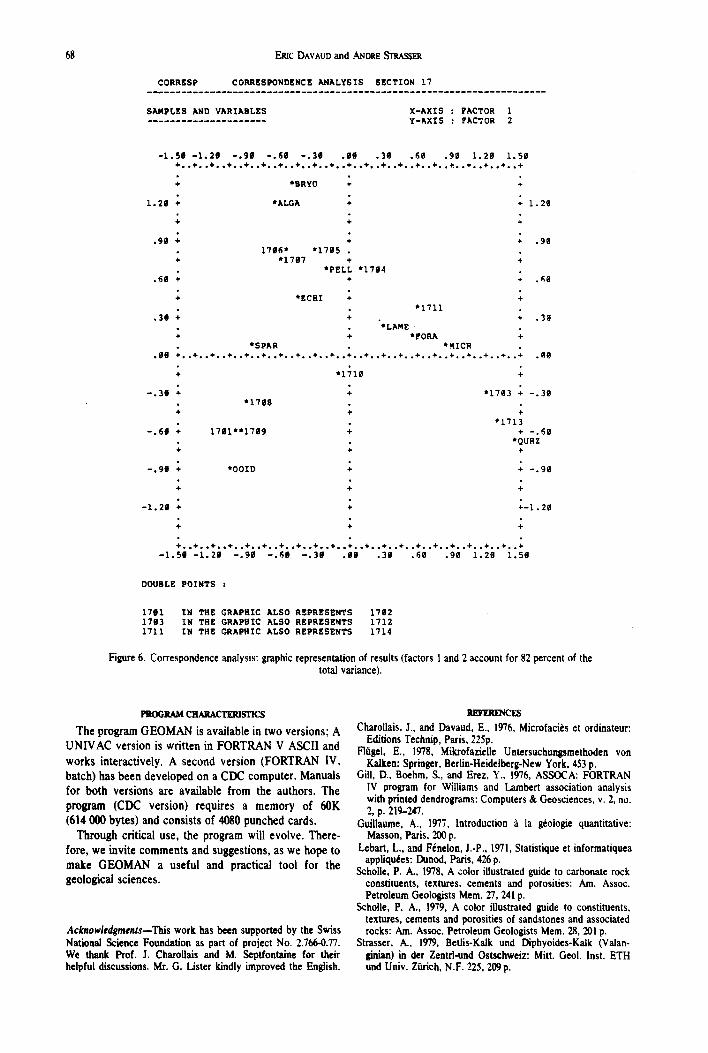
After a second preparation of 10 component frequen- cies, a correspondence analysis is performed (Fig. 6 shows the final results) and factors are calculated for samples and variables. Representation of results on a grid reveals groupings of samples and variables relative to the factor axes. For example, samples 1701, 1702, 1708, and 1709 (containing ooids) and the variable OOID form one group. For the statistical background and exact interpretation, refer to Lebart and Ftnelon (1971) and Guillaume (1977).

LOG HYPOTHSTICAL SSCTION 17 . . . . . . . . . . . . . . . . . . . . . . . . . . . . . . . . . . . . . . . . . . . . . . . . . . . . . . . . . . . . . . . . . . . . . .

SCALE 1 : 1 S I .

Illl : PlATR . . . . : 0URZ 0000 : PZLO ~mmm : BIOq

DEPTH SNSPLE

1 7 1 3

2 3 .

21.

1712

1711 19.

1718 1789

1 7 .

17g8

15. 1787

13.

1 1 . 17S6

9 .

17S5 7.

5.

17B4 1783

3 .

1782

1 . 17BI

CUgULATIVS LOGS PSLL 0OID ALGA BRYO

E. SS. g . 5 8 . I I I I . . . . . . . . . . . . . . . . . . I I . . . . . . . . I I . . . . . . . . 1 I I I I I I I I I I I I I - O 0 0 0 0 " - - - t t t e * * * I I I I I I I I I I . . . . . . . . . . " " + + I I I l l l I I I l l . . . . . . . . . . " " + + I I I I I I I I I I I . . . . . . . . . " " + + I I I I I I I I I I I . . . . . . . . . " ' " ÷ + I I I I I I I I I I I I . . . . . . . . . " " ÷ + I I I I I I I I I I I I . . . . . . . . " " + + I I I l l l l I l l I l . . . . . . . . " " + + I I I I I I l l l I I l l . . . . . . . " " + + I I I l l l l l l l I l l . . . . . . . " " ÷ + I I I I l l l l l I I l l . . . . . . . " " + + I I I I I I I I I I I I I I . . . . . . . " " " I I I l l l l l l I l l l l . . . . . . . - - + ÷ I I I l l l l l l l I I l l O 0 0 0 - - - - - * * * t * * I I I I I l l l l l I l l l O 0 0 0 - - - - - +÷+++ + I I I I l l l l l I I I I l O 0 0 0 0 - - - - , ÷ ÷ ÷+÷ I I I l l l I I I l l l I O 0 0 0 0 , . - - - - +÷+ ÷÷++ I I I I l l I l l l I l l O 0 0 0 0 0 - - - - * * * * t o * I I I I I I I l l O 0 0 0 0 0 O O 0 0 0 m m . * * * * * * * * * * * * I * * I I I I I I I I O 0 0 O O 0 0 0 0 0 0 - - - ++ + + ÷ + + + + + + + I ++ I I l l l l l l O 0 0 0 0 0 0 0 0 O u - m - ++ +++++++++ I ++ I I I I I I I I O O 0 0 0 0 0 0 0 0 - - - - * * * * t t * * t e * * I e * I I I l l l l lOOOOOO0000===- ÷ + + ÷ ÷ ~ ÷ ÷ ÷ ÷ ÷ ~ I ++ I ++ I I I I I I I I O O O O l m l . l g ~ m m ÷ + + + + I ÷ + I ++ I I I I I I I I O 0 0 0 ~ a ~ m l m + + ÷ + + I ÷+ I ÷÷ I l l l I I I l O O O O " ' ' ' ' ' ' " * ' * * * I * * I * " I l l l l l l I O 0 0 0 - g - - - - - - - ++++ + I ++ I ++ I I I I I I I I O O O O s - - - - - - - - + + + + + I ++ I ++ I I I I I I I I O C ~ S U m l l U m U l ÷ ÷ + + + I ÷ + I ÷+ I I l l l I I l O 0 0 0 m ' ' ' ' ' ' ' ' ÷÷++ ÷ I 4 + I ÷+ I I I I I I I I O C ~ O - - - - - - - - - +++÷ + I ÷÷ I ++ I I l l l I I l O 0 ~ - - ' ' - - ' - +++÷+ + I ÷+ I +÷ I I I I I Z I I O 0 0 0 m l . m l . s . . + + 4 + + + I ÷ 4 I ÷ + I I I I I I I I O 0 0 0 1 ~ g ~ S ~ l ~ ' + ÷ ÷ ÷ + + I ÷ ÷ I ÷ + I l l l l l l I O 0 0 0 " ' o m m - - ' - * * * * * * I e* I *e I I I I I I I I O 0 0 0 ' ' ' ' ' ' ' " + ÷ + + + + I ++ I ÷ + I I I I I I I I O O 0 0 0 - - - - - - - - + + + + + + I ++ I ++ I I I I I I I I 0 0 0 0 0 m g m ' = m ' " + ÷ + + + + + I ~+ I +÷ I I I I I I I l O 0 0 O O ~ m - - ' - ~ - + + + + + + + I ÷ + I ++ I I I I I I I I O 0 0 0 0 Q R . ~ . . . . . ÷ + + ÷ + + + I + ÷ I ++ l I I I I I I I O 0 0 0 0 0 " - ' ' ' ' - + ÷ + ÷ + + + ÷ I ++ I ++ I I I I I I I I 0 0 0 0 O O ~ = m = a m m + + + + + + + + I ++ I ++ I l l l ¿ I I I O 0 0 0 0 0 = = ~ m - - - + ÷ + + + + + + I + ÷ I ++ I I I I ¿ I I I O 0 0 0 0 0 0 t m s m ' m * * e , m * * * t I * * ! * ~ I i r i i i i I O O O O O O O l l ~ m m l ÷÷÷÷÷~÷4, , ÷ I ÷ ÷ I 4~ I l l l I I I l O O O O 0 0 0 ' ' ' ' ' ÷ ÷ + ÷ + + + ÷ + I ÷+ I ÷+ Z l l l I I I l O ~ O ' ' ' ' ' ++÷+++++ + I ++ I ++ I ¿ I I I I I ¿ O 0 0 0 0 0 0 - - - - - - + ÷ + + + + + + + I e-+ I ++ I l l l l l Z I l O ~ O 0 - ' ' " + + + + + ÷ + + + I ÷ + I ++ I I I l l l I l l O ~ O 0 0 0 m ~ - - - + + + + + + + + + I ++ I ++ I I I I I I I I I O 0 0 0 0 0 0 0 e m ' " +++++++÷+ + I ++ I ++ I I I I I I I I I 0 0 0 0 0 0 0 0 ' ' ' ' +++÷+++++ + I ++ I ÷+ I

• I * * I t l I I ¿ I I I I I I O 0 0 0 0 0 0 0 - - - - * * * * * * * * *

l l I ¿ l l l l I I l . . . . . . - - - * * • I I l l I l l l l I l l ¿ . . . . . . - - - + ÷ I I I I I I I I I I C ~ D O ~ + + * + + + + + + ÷ + + I I I I I I I I I I O O O O O O O O O O 0 0 " * * * * * * * * * * * * I I I I I I I I I I O O O 0 0 O O O O O 0 0 " +++ + + + + + + + + + I I 1 I I • I I I I 0 0 0 O O O O O O O O O " +++ + + ÷ + ÷ ÷ + ÷ + + I I 1

e l l l l I ¿ l O ~ O 0 0 0 0 0 0 0 0 " t * * * * * * * * * * ~ I I I

Figure 5. Distribution of variables in the geological section (Fig. 4): cumulative, singJe variable, and binary logs (the + to the right of sample 1713 indicates that there is insufficient room to print closely-spaced sample 1714).

• d 60Z '~ZC ":IIN 'q~.u.n.Z "^.mfl pun HI~ "~SUl "1o¢9 'n!!~ :z!a~sq~slsO pun-l.~UO z a~p u! (u .en.~. -u¢leA) ~leN-sop!o,~qd~ pun ~le~I-S!lloB '6L6! "V 'Joss~lS

"d lO~ '8E 'moI~ s~S~OlO~ O mnoloJ~ad "~ossv "uric :s~poz po~e!~osse pue sauo~spues jo sop!soJod pue s~uomo~ 's~mlx~l 's:lu~nl.tlsuo~ ol op]n~ polvalSnll! JOlO:) V '6L61 "V "d 'allOq~

• d ll, Z '/.Z "tua~ sls.~olO~ 0 mnolonO d • ~oss V "uJ~ :s~.ll!SoJod pue SIuomo~ 's~.ml'¢o] 'slu:~nlQsUO~

• d 9~ 's.ued 'pouno :s~nb!ldde e~nbpetuJo,m! ~o ~nb!~sgel $ 'IL61 "d-T 'UOlOU,acI pue '"] '~eq~'- I

• d 00~ 'S.Lred 'uossel~ :~^.~e~!~u~nb a.~OlO,~ el e uop~npo~lu I 'LL6I "V 'amn~IBnO

"L~-6I~ "d '~ • ou '~ "^ 'so~uo!~soo 0 ~ s~omdmo D :~uJe~oJpuop p~mud W!M s!sAleu~ uo!~e!~osse lJaqme" 1 pue sme!ll!A~ Joj tue.~oJd AI NVHI~IOd :VDOSSV '9/61 "h 'zaa3 pue "S 'tuqa°8 "G 'll!O

"d £ft '~oA t6aN-$~llaP!aH-U!l~O~ 'aaSu!~ds :ua~)l uo^ uopoql~msSunq~nsJamfl ~llarZ~jO.nl.[EI '8/.61 "H 'l~$.n.L:l

"dfz z 's!~ d 'd.mq~al suo.I)!p 3 :maleu.tpJo lo s~!oeJoJ~!~ '9L61 "~1 'pne^e(] pue "f 'S!qlox~qD

glDNmi~dl~

"qs!#u~] aql po^oJdtu! Xlpupl ~als.r I 'D '.P~I 'suo!ssn:)s!p ln~dlO q a!a W ,oj ~u.nnuot;d~S "I~I pue S~lloxeqD '~ "joM ~lmnll ~A~ "L£'0-99/.'~ "oN l~[oJd jo lzed se uopepuno:l ~uo!~S l~uo.~N ss!m S aql ,~q p~oddns U~l seq ~pom S.nL]--s~uam~pals~Omla¥

oql Joj IOOl le~9~ezd pue Injosn e NTV~O,~E) oTem ol odoq ~ se 'suo!1sa~ns pue sluomtuo~ ~l!^u! ~ 'oJoj -aaaqI "a^lO^a II!~ me,~oJd aq; 'asn leO!l.uo q'SnoJtLL

• spJeo p~q~und 0g0], jo s]s!suoo pue (s~lXq 000 1'!9) ){09 JO AJom~m e so.lmboJ (UO!S.10^ :)a3) ll~.l~O,Id ~qI "sJoqme ~ql mozj ~iqel.m^e ~ze suo!sJ~^ q~oq JoJ slenueI~ "J~mdmo~ :KID e uo p~dol~^O p uo~q seq (q31eq 'AI NV~IIHOrl) uo!s.m^ puo~os V "AI~Ap~J01U! S~.lOt~ pue IIDSV A NV~IIHOd u! u~1l.u~ s! uolsJ~^ DVAIN~I V 'suo! sJ~^ o~1 u! ~lqel~^~ s! NVI~O~ID tue~md ~qi

SDLLqFd~IDVHVH3 Iq'C~OOid

• (o~ue.ue^ lelOl a W jo ]uo~J~ Z8 zoj 1unooae Z pue I szol3ej) sllns;J jo uo.~lu~oJdoJ :~.tqdv,.C8 :s!sXleUe a~uapuodsa.uo D "9 om$!d

PILl SLN3SIad3B OS~Y OlHd~aO 3H& NI fILl ZILI B&N3SI~d38 OS~Y DIHdV~O 3H& NI £BLI fILl S&NaSiada~ OSqY DIHdVa5 3H& HI I~LI

: S&NXOd X~gflOU

+o,÷o.÷o,+oo~*'+oo+°'+,-÷.o÷o,+-,+o~÷o~+,,+°o÷~,÷°,+~.÷*°÷,.÷

+

~" I-+

+

~6"- +

+

~9"- +

o£--

o~-

e£"

~6" ÷

EZ'I +

£1LI~

+ E~LI~

+

÷

+

÷

+

~..÷..+l.÷..+o.+..+..+..+..+.

÷

fILl* +

~0LI~

+o-+-.+,,÷,.%,-÷..+o,+,.+,,+.

BS°I BZ'I B6" B9" BE"

+ BZ'I-

÷

aloo, + o6"-

+

6BLI~IILI + e9"-

+

8mLI~ ÷ 0£ ° -

+

• +..+..+..+..+o .+. o+..÷..+. -+..÷ DB °

+ ÷

+ + e£"

+ IHDI, +

+ 09"

+ L%LI~ ÷

• ~BLI, wgmLI + + 16"

÷ ÷

+ YS~Y~ + eZ'%

+ O~Q~ +

o+..+..+..+..+-.~..+--~..+.-+.-÷

00" D{'- Jg"- 16"- BI'I- 0~'I-

~O&3W3 : SIX¥-~ ..................... I aO&3¥~ : S2XV-X $~gYI~Y^ ON¥ $3~d~S

......................................................................

L~ HOILDIS SIS~YHV ZDN~ONOdSZ~O3 dS~WHO~

~ ~aNV pwe anvAV(l ~rcH 89