Geometric Correction, Orthorectification, and Mosaickingjohnbull.weebly.com/uploads/2/5/3/7/25376223/bulljgisc9216d3.pdf · Geometric Correction and Mosaicking thMarch 12 , 2014 14

Geometric Correction, Orthorectification, and Mosaicking

For: Janet Finlay

GISC9216- Digital Image Processing

John Bull

B.Sc Candidate

GIS-GM Candidate

3 Jasmin Crescent

St. Catharines, Ontario

Table of Contents 1. Introduction .......................................................................................................................................... 1

2. Methodology ......................................................................................................................................... 2

2.1. Polynomial Correction .................................................................................................................. 6

2.2. Polynomial Model Mosaic ........................................................................................................... 13

2.3. Orthorectification ....................................................................................................................... 17

2.4. Orthorectification Mosaic ........................................................................................................... 22

3. Analysis ............................................................................................................................................... 23

3.1. Polynomial Model Mosaic Results .............................................................................................. 23

3.2. Orthorectification and Mosaic .................................................................................................... 27

Conclusions ................................................................................................................................................. 32

Bibliography ................................................................................................................................................ 33

Figure 1: Original air photo to be used as reference image ........................................................................ 2

Figure 2: Photo 1 to be rectified ................................................................................................................... 3



Figure 5: Control points button initiating geometric correction procedure ................................................. 6

Figure 6: Example of ground control points................................................................................................. 7

Figure 7: Close look at placement of a ground control point ....................................................................... 8

Figure 8: Fourth ground control point accuracy ........................................................................................... 9

Figure 9: RMS error examples ..................................................................................................................... 10

Figure 10: Prediction of eighth ground control point ................................................................................. 11

Figure 11: Resample dialog box .................................................................................................................. 12

Figure 12: Resampled photo overlaid on reference image ........................................................................ 13

Figure 13: Mosaic Express ........................................................................................................................... 14

Figure 14: Mosaic Express dialog box ......................................................................................................... 14

Figure 15: Input area tab from mosaic wizard ............................................................................................ 15

Figure 16: Colour corrections in mosaic ..................................................................................................... 16

Figure 17: Mosaicked image of geometrically corrected photos using the polynomial model ................. 17

Figure 18: Camera model properties dialog box ........................................................................................ 18

Figure 19: Fiducial placement and dialog box ............................................................................................ 19

Figure 20: RMS errors in an orthorectified photo ...................................................................................... 20

Figure 21: Resample dialog box for orthorectification ............................................................................... 20

Figure 22: Resampled aerial photo using orthorectification ...................................................................... 21

Figure 23: Orthorectified mosaic overlaid on reference image .................................................................. 22

Figure 24: Misaligned roads in polynomial mosaic ..................................................................................... 24

Figure 25: Colour changes and errors in mosaic result............................................................................... 25

Figure 26: Top half of polynomial mosaic result ......................................................................................... 26

Figure 27: Road network misalignment and buildings displaced ............................................................... 27

Figure 28: Orthorectification showing road networks lining up ................................................................. 28

Figure 29: Comparison of elevation distortion between polynomial model and orthorectification ......... 29

Figure 30: Slight difference in colour between mosaic and reference image ............................................ 30

Figure 31: Overlay of vector layers onto orthorectified mosaic ................................................................. 31

Figure 32: Road networks lining up well with mosaic result ...................................................................... 31

Geometric Correction and Mosaicking March 12th, 2014

1

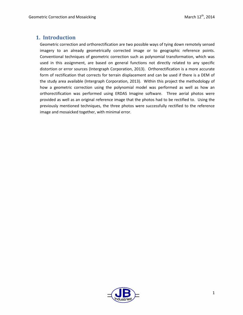
1. Introduction Geometric correction and orthorectification are two possible ways of tying down remotely sensed

imagery to an already geometrically corrected image or to geographic reference points.

Conventional techniques of geometric correction such as polynomial transformation, which was

used in this assignment, are based on general functions not directly related to any specific

distortion or error sources (Intergraph Corporation, 2013). Orthorectification is a more accurate

form of rectification that corrects for terrain displacement and can be used if there is a DEM of

the study area available (Intergraph Corporation, 2013). Within this project the methodology of

how a geometric correction using the polynomial model was performed as well as how an

orthorectification was performed using ERDAS Imagine software. Three aerial photos were

provided as well as an original reference image that the photos had to be rectified to. Using the

previously mentioned techniques, the three photos were successfully rectified to the reference

image and mosaicked together, with minimal error.


2

2. Methodology The methodology section outlines how both the geometric correction as well as the

orthorectification were performed in the ERDAS Imagine software. The original reference image

can be seen below in Figure 1.

Figure 1: Original air photo to be used as reference image


3

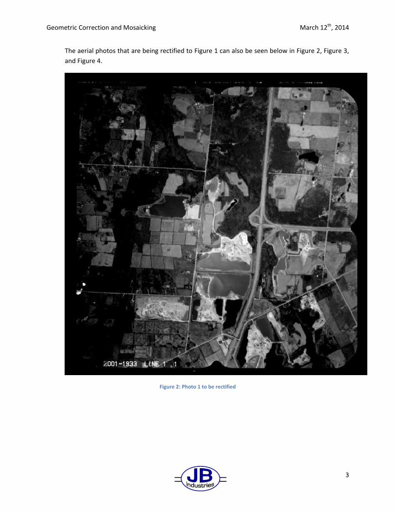
The aerial photos that are being rectified to Figure 1 can also be seen below in Figure 2, Figure 3,

and Figure 4.

Figure 2: Photo 1 to be rectified


4



5



6

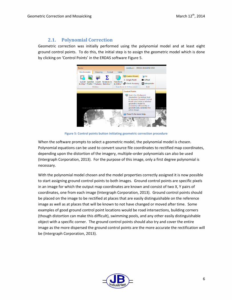
2.1. Polynomial Correction Geometric correction was initially performed using the polynomial model and at least eight

ground control points. To do this, the initial step is to assign the geometric model which is done

by clicking on ‘Control Points’ in the ERDAS software Figure 5.

Figure 5: Control points button initiating geometric correction procedure

When the software prompts to select a geometric model, the polynomial model is chosen.

Polynomial equations can be used to convert source file coordinates to rectified map coordinates,

depending upon the distortion of the imagery, multiple-order polynomials can also be used

(Intergraph Corporation, 2013). For the purpose of this image, only a first degree polynomial is

necessary.

With the polynomial model chosen and the model properties correctly assigned it is now possible

to start assigning ground control points to both images. Ground control points are specific pixels

in an image for which the output map coordinates are known and consist of two X, Y pairs of

coordinates, one from each image (Intergraph Corporation, 2013). Ground control points should

be placed on the image to be rectified at places that are easily distinguishable on the reference

image as well as at places that will be known to not have changed or moved after time. Some

examples of good ground control point locations would be road intersections, building corners

(though distortion can make this difficult), swimming pools, and any other easily distinguishable

object with a specific corner. The ground control points should also try and cover the entire

image as the more dispersed the ground control points are the more accurate the rectification will

be (Intergraph Corporation, 2013).


7

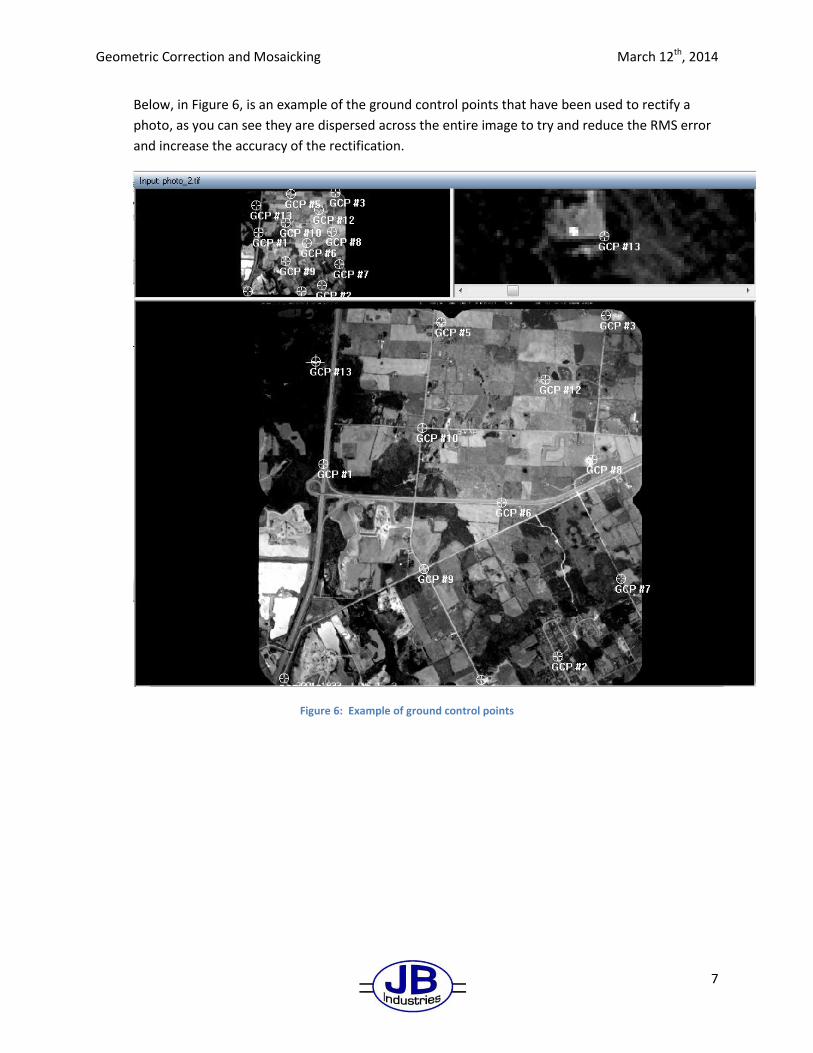
Below, in Figure 6, is an example of the ground control points that have been used to rectify a

photo, as you can see they are dispersed across the entire image to try and reduce the RMS error

and increase the accuracy of the rectification.

Figure 6: Example of ground control points


8

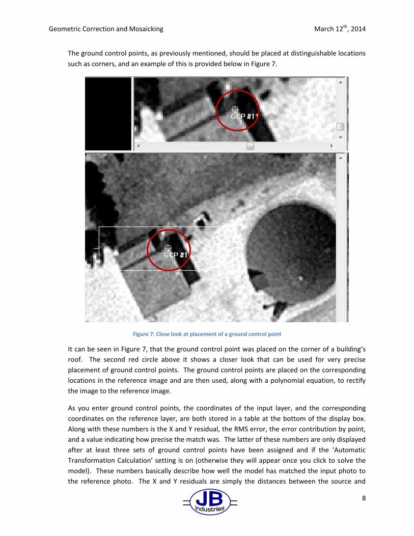
The ground control points, as previously mentioned, should be placed at distinguishable locations

such as corners, and an example of this is provided below in Figure 7.

Figure 7: Close look at placement of a ground control point

It can be seen in Figure 7, that the ground control point was placed on the corner of a building’s

roof. The second red circle above it shows a closer look that can be used for very precise

placement of ground control points. The ground control points are placed on the corresponding

locations in the reference image and are then used, along with a polynomial equation, to rectify

the image to the reference image.

As you enter ground control points, the coordinates of the input layer, and the corresponding

coordinates on the reference layer, are both stored in a table at the bottom of the display box.

Along with these numbers is the X and Y residual, the RMS error, the error contribution by point,

and a value indicating how precise the match was. The latter of these numbers are only displayed

after at least three sets of ground control points have been assigned and if the ‘Automatic

Transformation Calculation’ setting is on (otherwise they will appear once you click to solve the

model). These numbers basically describe how well the model has matched the input photo to

the reference photo. The X and Y residuals are simply the distances between the source and


9

retransformed coordinates, whereas the RMS error is the root-mean-square of the X and Y

residuals added together; this gives a reasonable estimate of the overall error.

When the fourth ground control point is placed on the input image, the model automatically

generates a corresponding ground control point on the reference image. In most cases this

corresponding ground control point won’t be very accurate but should be in the vicinity of where

it should be. Figure 8 below shows an example of a corresponding fourth ground control point,

the red circle indicates as to where the ground control point should actually be placed.

Figure 8: Fourth ground control point accuracy

As mentioned before, the prediction process for the ground control points will rarely be exact

because the model’s inputs are always going to have a slight amount of error. Whether it be that

the placement of the ground control points is slightly off, or that they are not placed in a way that

gives a complete spatial coverage of the image, error will always exist in the inputs, and therefore

the output will also always have error. The goal in this process is to minimize the error as much as

possible.


10

Within this project, an RMS error of less than 0.1 was maintained to ensure an accurate

rectification of the images. An example of the RMS error ranges that were encountered using the

polynomial model can be seen below in Figure 9.

Figure 9: RMS error examples


11

The more ground control points that are entered, the better the prediction process will become,

as long as the new ground control points are accurate. A total of eight ground control points were

used for each photo; by the eighth ground control point, the prediction process is much more

accurate as it has more inputs to work with. Error! Not a valid bookmark self-reference. below

shows the prediction result of the eighth ground control point assigned.

The top-right corner of this house was chosen in the left image as the ground control point, and it

can be seen in the right image that the prediction process was very accurate in placing the

corresponding control point on the reference image, far more accurate than what was seen in

Figure 8.

Figure 10: Prediction of eighth ground control point


12

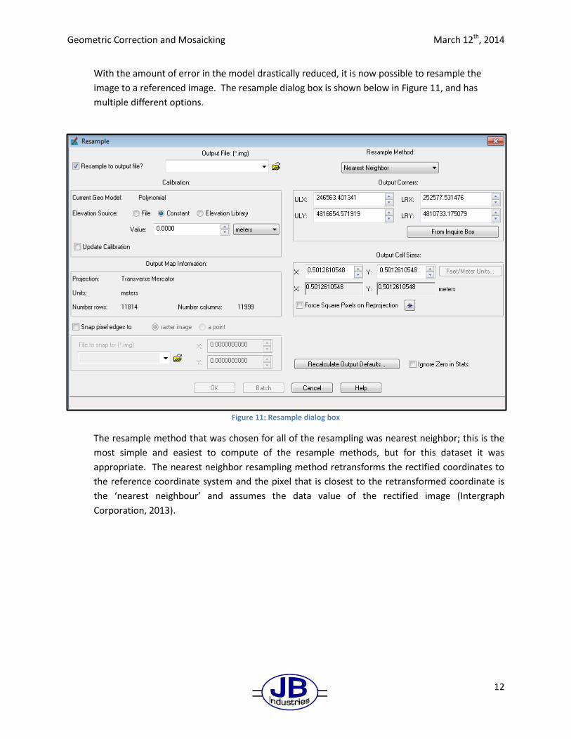
With the amount of error in the model drastically reduced, it is now possible to resample the

image to a referenced image. The resample dialog box is shown below in Figure 11, and has

multiple different options.

The resample method that was chosen for all of the resampling was nearest neighbor; this is the

most simple and easiest to compute of the resample methods, but for this dataset it was

appropriate. The nearest neighbor resampling method retransforms the rectified coordinates to

the reference coordinate system and the pixel that is closest to the retransformed coordinate is

the ‘nearest neighbour’ and assumes the data value of the rectified image (Intergraph

Corporation, 2013).

Figure 11: Resample dialog box


13

With the resample method chosen and the output file selected, all other parameters were left as

is. By pressing ‘OK’ the rectified image is resampled onto the reference image and results in what


Figure 12: Resampled photo overlaid on reference image

2.2. Polynomial Model Mosaic Once all of the three photos went through the rectification process outlined previously, they were

ready to be mosaicked together into one continuous image. The mosaic process can be easily


14

done in the ERDAS software using the Mosaic Express wizard which can be seen below in Figure

13.

Figure 13: Mosaic Express

By clicking on the Mosaic Express button, the mosaic dialog box can be opened Figure 14.

Figure 14: Mosaic Express dialog box

Within this dialog box, the parameters for the mosaic can be set and any colour manipulation or

cropping can be done within the wizard. The three rectified air photos were loaded into the Input


15

tab first, as can be seen in Figure 14. Secondly, the input area was adjusted so that the black area

around the air photo, as well as the fiducial marks, would be eliminated from the mosaic image

Figure 15.

Figure 15: Input area tab from mosaic wizard

The crop area was set to 18% after some trial and error in an attempt to cut out as little of the

actual image as possible. With the cropping complete, colour corrections were also made since

each of the air photos had a slightly different brightness value range.


16

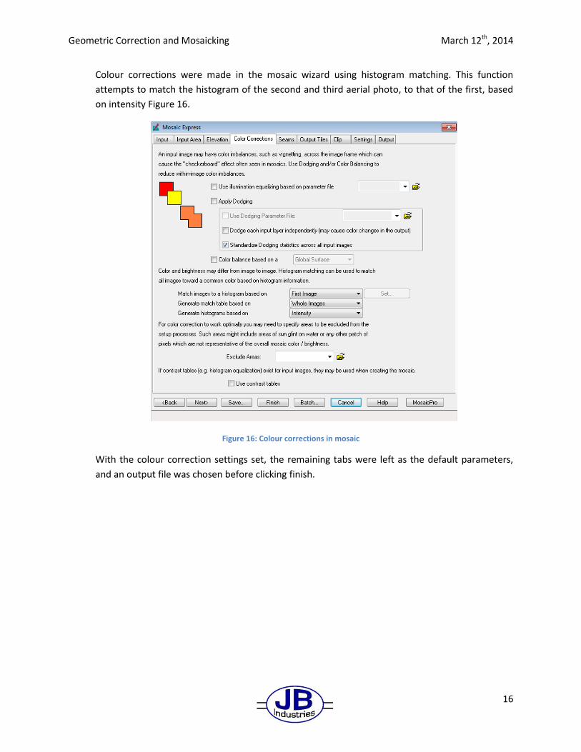
Colour corrections were made in the mosaic wizard using histogram matching. This function

attempts to match the histogram of the second and third aerial photo, to that of the first, based

on intensity Figure 16.

Figure 16: Colour corrections in mosaic

With the colour correction settings set, the remaining tabs were left as the default parameters,

and an output file was chosen before clicking finish.


17

The final mosaicked output can be seen below in Figure 17.

Figure 17: Mosaicked image of geometrically corrected photos using the polynomial model

2.3. Orthorectification The second form of geometric correction that was performed on the aerial photos was

orthorectification. Orthorectification is a form of rectification that corrects for distortion

associated to terrain displacement and can be used if there is a digital elevation model of the


18

study area (Intergraph Corporation, 2013). A digital elevation model was provided within the

project’s data and this was used along with provided parameters for the aerial sensor.

To begin the orthorectification process, the ‘Control Points’ button must once again be clicked to

open up the geometric model dialog box. Instead of using the polynomial model, this time we will

select ‘Camera’ as we have the associated parameters for the sensor used to take these photos.

With ‘Camera’ selected as the geometric model, the ground control point selection screen once

again opens along with the camera model properties. The camera model properties dialog box


Figure 18: Camera model properties dialog box

The first step in the camera model properties box is to set the elevation source that will be used,

which in this case is the previously mentioned digital elevation model. After navigating to the

elevation model, we can fill out the rest of the parameters that were provided. The provided

principal points were zero for both X and Y, while the focal length was 152.468mm; we were also

told to use five iterations in the correction process. The next step is to navigate to the ‘Fiducials’

tab and identify the fiducials on the input photo so that the geometric model knows the location

of the principle point in the aerial image. This is done in the same way as ground control points

by placing a crosshair on the appropriate location. The aerial images that are being used have

eight fiducials which were all marked, and the provided Film X and Film Y values were inputted

(Figure 19).


19

The provided Film X and Film Y values can be seen in the right side of Figure 19, whereas the left

side of the image shows a fiducial mark as well as the placement of a cross hair in the middle of it.

With the fiducial marks correctly placed, and all other parameters completed, ground control

points are once again required to complete the orthorectification process. The orthorectification

process is a much more accurate model than the polynomial model due to the accuracy of the

parameters being inputted, as well as the usage of the digital elevation model, however, accurate

ground control points still need to be used. Only four sets of ground control points are required

for the orthorectification process as opposed to the eight needed for the geometric correction

using the polynomial model. Unlike the polynomial model, once you reach the fourth ground

control point, a corresponding, predicted, ground control point does not appear on the reference

image; this control point must be manually placed. With the four ground control points placed,

the ‘Solve Geometric Model’ button can be clicked and the residuals and errors will once again be

visible.

Figure 19: Fiducial placement and dialog box


20

Figure 20 below shows an example of the RMS errors in an orthorectified photo using only four

ground control points.

Figure 20: RMS errors in an orthorectified photo

It can be seen that the RMS errors of 0.001 and 0.002 are far smaller than any of the RMS error

values we hoped to get in the geometric correction using the polynomial model meaning that we

are likely to get a far more accurate rectification.

With enough ground control points chosen, the photo is ready to be resampled to the reference

image. The resample dialog box is once again shown below in Figure 21.

Figure 21: Resample dialog box for orthorectification

The previously described resampling method of nearest neighbor will once again be used in the

resample, and the only other major difference in this dialog box is that the geometric model is set

to ‘Camera’ and makes reference to an elevation source, whereas the polynomial model did not.


21

After pressing ‘OK’ the image is resampled and can be placed on top of the original reference

image (Figure 22).

Figure 22: Resampled aerial photo using orthorectification


22

2.4. Orthorectification Mosaic With the three photos rectified to the reference image using orthorectification, they can now be

mosaicked together into one image using the same process as earlier described. The

orthorectification mosaic used the exact same dialog parameters as the polynomial model

regarding cropping, and colour corrections. The orthorectified mosaic can be seen below in

Figure 23.

Figure 23: Orthorectified mosaic overlaid on reference image


23

3. Analysis Once the geometric correction has been done to the aerial photos, once using a polynomial

model, and another time using orthorectification, the photos must be visually analyzed to assess

the quality of the rectification. The most common areas to look for errors are near the edges of

the mosaic, where the photo edge meets the reference image edge. Linear features like roads

and bridges are generally used as baselines for the amount of error that is seen in a rectification

result. Other errors such as colour imbalances can also be seen through a visual inspection of the

mosaic.

Another common way to check for errors is to overlap referenced vector data on top of the

mosaic and to visually inspect how it lines up. For this project we were provided with a roads and

a buildings vector layer that will be used to compare the results of the rectifications.

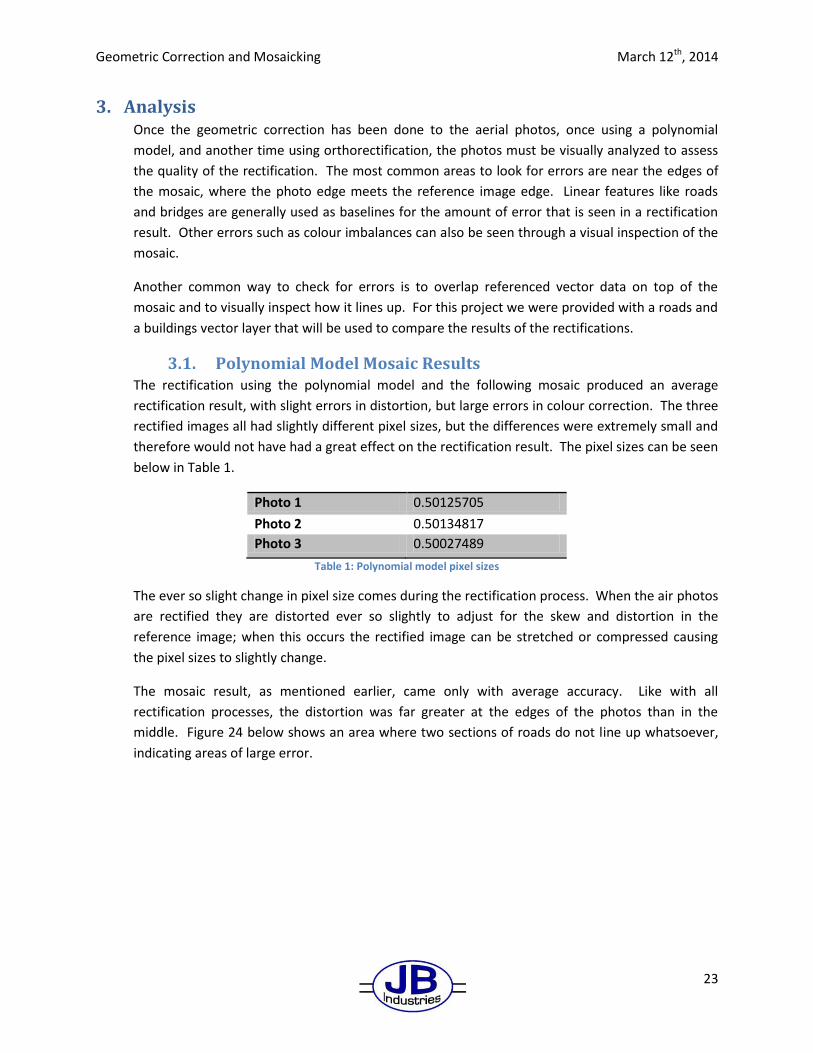
3.1. Polynomial Model Mosaic Results The rectification using the polynomial model and the following mosaic produced an average

rectification result, with slight errors in distortion, but large errors in colour correction. The three

rectified images all had slightly different pixel sizes, but the differences were extremely small and

therefore would not have had a great effect on the rectification result. The pixel sizes can be seen

below in Table 1.

Photo 1 0.50125705

Photo 2 0.50134817

Photo 3 0.50027489

Table 1: Polynomial model pixel sizes

The ever so slight change in pixel size comes during the rectification process. When the air photos

are rectified they are distorted ever so slightly to adjust for the skew and distortion in the

reference image; when this occurs the rectified image can be stretched or compressed causing

the pixel sizes to slightly change.

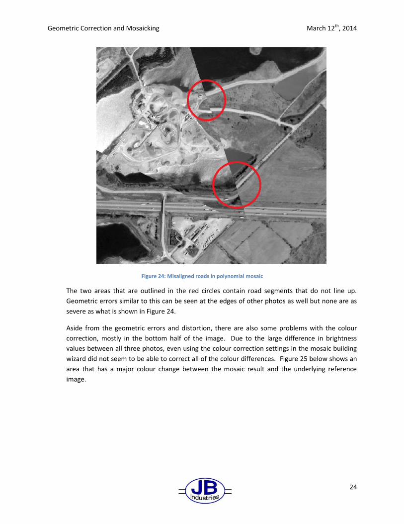
The mosaic result, as mentioned earlier, came only with average accuracy. Like with all

rectification processes, the distortion was far greater at the edges of the photos than in the

middle. Figure 24 below shows an area where two sections of roads do not line up whatsoever,

indicating areas of large error.


24

Figure 24: Misaligned roads in polynomial mosaic

The two areas that are outlined in the red circles contain road segments that do not line up.

Geometric errors similar to this can be seen at the edges of other photos as well but none are as

severe as what is shown in Figure 24.

Aside from the geometric errors and distortion, there are also some problems with the colour

correction, mostly in the bottom half of the image. Due to the large difference in brightness

values between all three photos, even using the colour correction settings in the mosaic building

wizard did not seem to be able to correct all of the colour differences. Figure 25 below shows an

area that has a major colour change between the mosaic result and the underlying reference

image.


25

Figure 25: Colour changes and errors in mosaic result

The top half of the image was rectified with a little more accuracy; however, small geometric and

radiometric errors still occurred. Figure 26 below shows the top half of the mosaic result with

some smaller errors outlined in red circles.


26

Figure 26: Top half of polynomial mosaic result

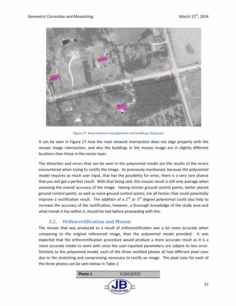
After visually inspecting the results, the roads and buildings vector layers were draped over the

mosaic to compare how they line up to the mosaic results. For the most part, the vector layer

corresponded with the mosaic result very well, with road networks lining up, but the buildings

were slightly displaced, depending on which section of the mosaic you were looking in. The area

of the mosaic where photo 2 was located had the most errors as can be seen below in Figure 27.


27

Figure 27: Road network misalignment and buildings displaced

It can be seen in Figure 27 how the road network intersection does not align properly with the

mosaic image intersection, and also the buildings in the mosaic image are in slightly different

locations than those in the vector layer.

The distortion and errors that can be seen in the polynomial model are the results of the errors

encountered when trying to rectify the image. As previously mentioned, because the polynomial

model requires so much user input, that has the possibility for error, there is a very rare chance

that you will get a perfect result. With that being said, this mosaic result is still only average when

assessing the overall accuracy of the image. Having stricter ground control points, better placed

ground control points, as well as more ground control points, are all factors that could potentially

improve a rectification result. The addition of a 2nd or 3rd degree polynomial could also help to

increase the accuracy of the rectification, however, a thorough knowledge of the study area and

what trends it has within it, should be had before proceeding with this.

3.2. Orthorectification and Mosaic The mosaic that was produced as a result of orthorectification was a lot more accurate when

comparing to the original referenced image, than the polynomial model provided. It was

expected that the orthorectification procedure would produce a more accurate result as it is a

more accurate model to work with since the user-inputted parameters are subject to less error.

Similarly to the polynomial model, each of the three rectified photos all had different pixel sizes

due to the stretching and compressing necessary to rectify an image. The pixel sizes for each of

the three photos can be seen below in Table 2.

Photo 1 0.50110725


28

Photo 2 0.50055173

Photo 3 0.49999564

Table 2: Pixel sizes for orthorectified aerial photos

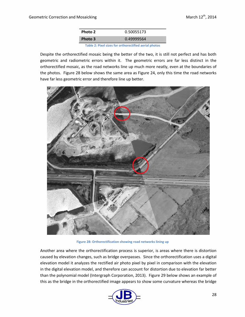
Despite the orthorectified mosaic being the better of the two, it is still not perfect and has both

geometric and radiometric errors within it. The geometric errors are far less distinct in the

orthorectified mosaic, as the road networks line up much more neatly, even at the boundaries of

the photos. Figure 28 below shows the same area as Figure 24, only this time the road networks

have far less geometric error and therefore line up better.

Figure 28: Orthorectification showing road networks lining up

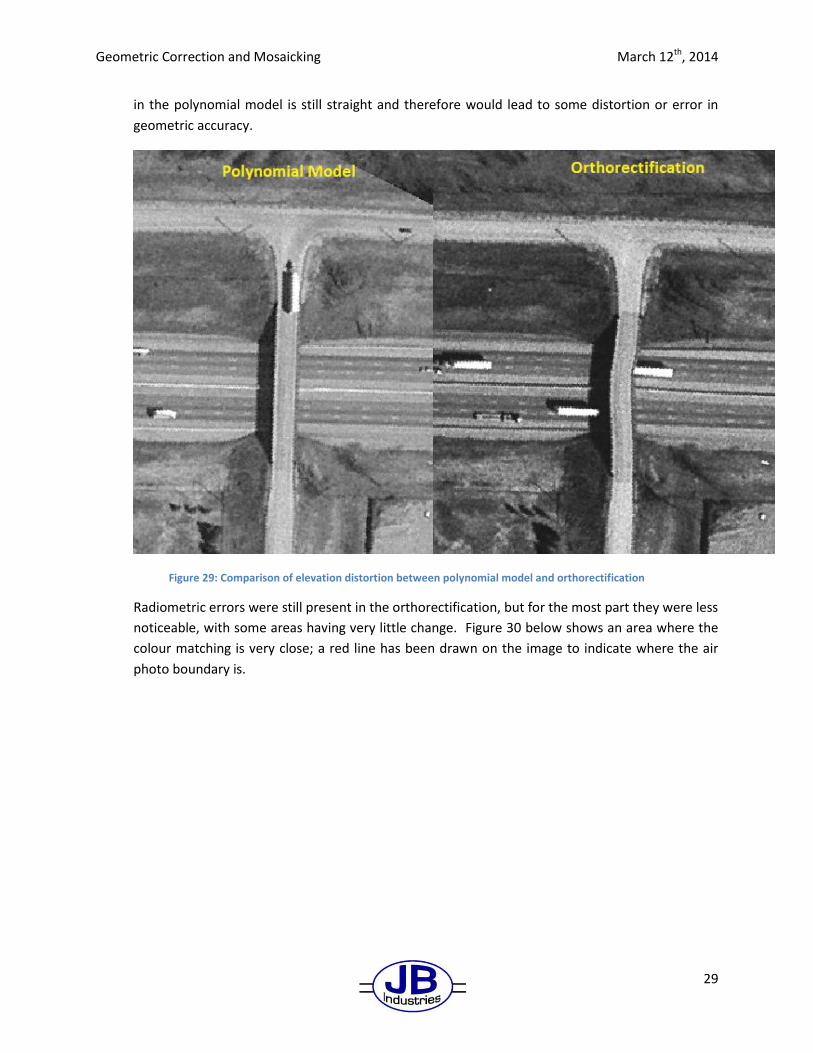
Another area where the orthorectification process is superior, is areas where there is distortion

caused by elevation changes, such as bridge overpasses. Since the orthorectification uses a digital

elevation model it analyzes the rectified air photo pixel by pixel in comparison with the elevation

in the digital elevation model, and therefore can account for distortion due to elevation far better

than the polynomial model (Intergraph Corporation, 2013). Figure 29 below shows an example of

this as the bridge in the orthorectified image appears to show some curvature whereas the bridge


29

in the polynomial model is still straight and therefore would lead to some distortion or error in

geometric accuracy.

Figure 29: Comparison of elevation distortion between polynomial model and orthorectification

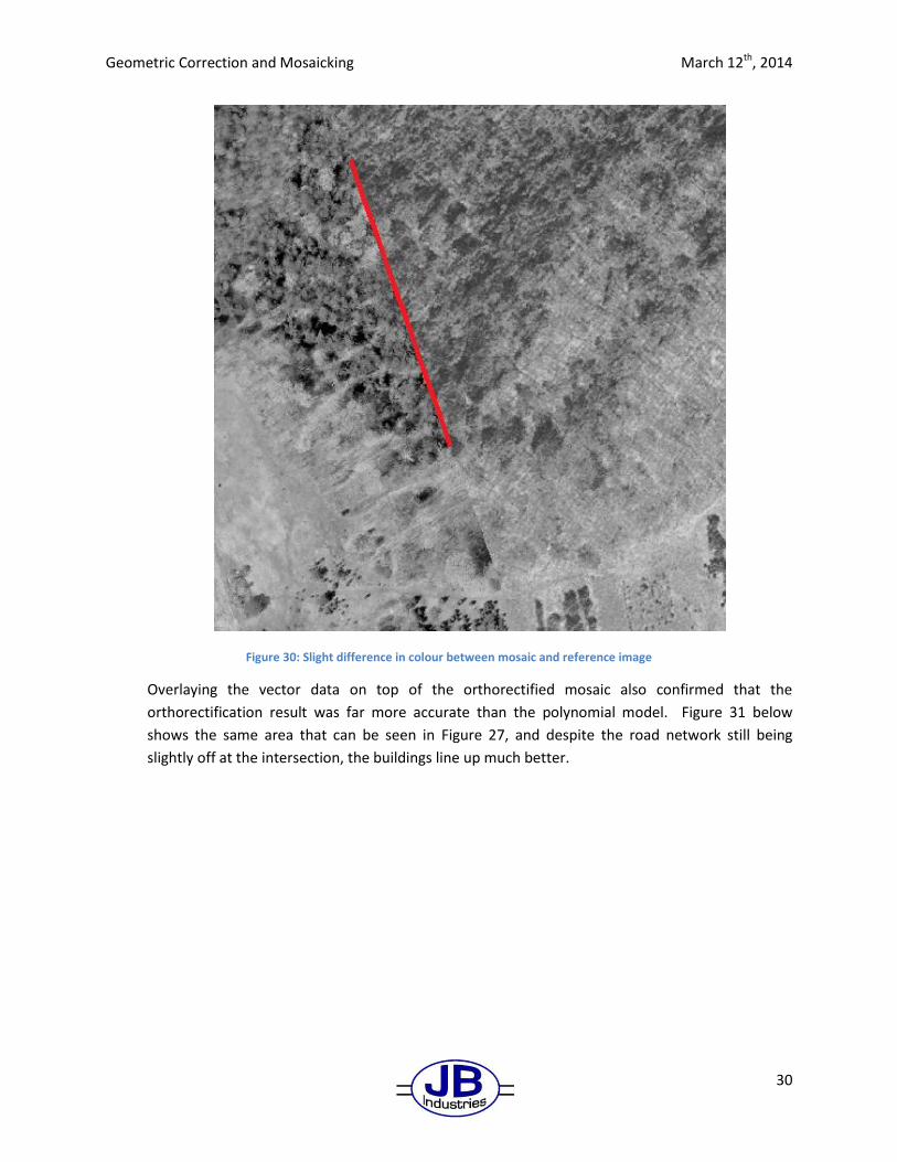
Radiometric errors were still present in the orthorectification, but for the most part they were less

noticeable, with some areas having very little change. Figure 30 below shows an area where the

colour matching is very close; a red line has been drawn on the image to indicate where the air

photo boundary is.


30

Figure 30: Slight difference in colour between mosaic and reference image

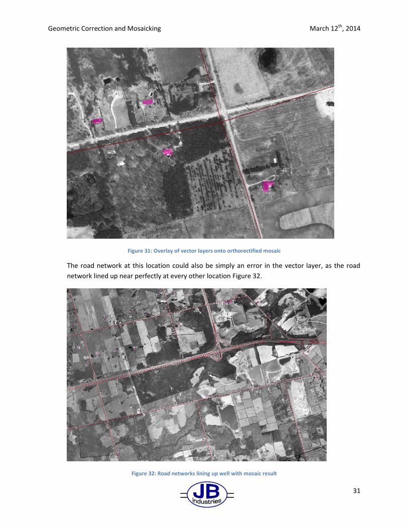
Overlaying the vector data on top of the orthorectified mosaic also confirmed that the

orthorectification result was far more accurate than the polynomial model. Figure 31 below

shows the same area that can be seen in Figure 27, and despite the road network still being

slightly off at the intersection, the buildings line up much better.


31

Figure 31: Overlay of vector layers onto orthorectified mosaic

The road network at this location could also be simply an error in the vector layer, as the road

network lined up near perfectly at every other location Figure 32.

Figure 32: Road networks lining up well with mosaic result


32

It can be seen in this image that the road network at many other locations lines up near perfectly.

In all, the orthorectification result produced a far more accurate and reliable rectification result

than the polynomial model. Geometric errors such as roads not lining up or other geometric

distortions were visibly reduced when using orthorectification and the overlay of vector data also

was aligned far more accurately.

Conclusions The goal of this project was to create two new rectified and mosaicked images, using two

different geometric models, in order to see which one produced a better result. Overall, it can

definitely be said that the orthorectification gave a far more accurate and aesthetically pleasing

result than the polynomial model did. Both geometric and radiometric distortion was reduced

gradually when comparing the two different models to the reference image, as well as to

referenced vector layers.

The reasoning behind this is that the orthorectification procedure uses more inputs, and more

accurate inputs, to create its output. The polynomial model relies very heavily on the assignment

of ground control points when it creates its rectified image, and therefore if the ground control

points are not exact, or are not spread throughout the image, it is far easier to receive greater

geometric errors. The orthorectification model uses an additional input, a digital elevation model,

to increase the accuracy and reduce distortion caused by elevation changes. The inputs for the

orthorectification model are also more concrete, in that the fiducials and camera parameters are

set in stone and are not up for personal opinion as some ground control points may be.

Both geometric correction models worked successfully, allowing the three aerial photos to be

rectified and mosaicked together, and then placed on top of the reference image with relative

success but in the future the orthorectification model would be chosen as the superior model

when dealing with this dataset.


33

Bibliography Intergraph Corporation. (2013). ERDAS Field Guide (October 2013 ed.). Huntsville, AL, United States of

America: Unpublished.

Documents

Geometric Correction, Orthorectification, and Mosaickingjohnbull.weebly.com/uploads/2/5/3/7/25376223/bulljgisc9216d3.pdf · Geometric Correction and Mosaicking thMarch 12 , 2014 14