Embed Size (px)
Citation preview
Geometric Modeling Summer Semester 2012
Dimensionality Reduction, Intrinsic Geometry and Discrete
Differential Operators
Dimensionality Reduction
Fitting Affine Subspaces
The following problem can be solved exactly:
• Best fitting line to a set of 2D, 3D points
• Best fitting plane to a set of 3D points
• In general: Affine subspace of ℝ𝑑, with dimension 𝑑 ≤𝑚 that best approximates a set of data points 𝐱𝑖 ∈ ℝ𝑚.
This will lead to the - famous - principle component analysis (PCA).
Start: 0-dim Subspaces
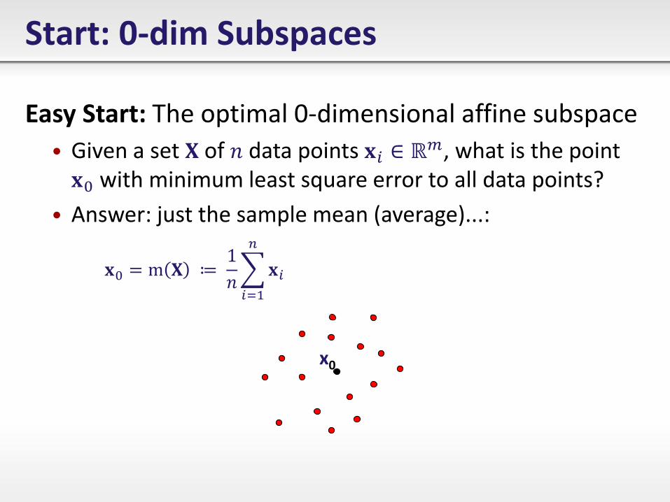
Easy Start: The optimal 0-dimensional affine subspace
• Given a set 𝐗 of 𝑛 data points 𝐱𝑖 ∈ ℝ𝑚, what is the point 𝐱0 with minimum least square error to all data points?
• Answer: just the sample mean (average)...:
x0
𝐱0 = m 𝐗 ≔ 1
𝑛 𝐱𝑖
𝑛
𝑖=1
One Dimensional Subspaces...
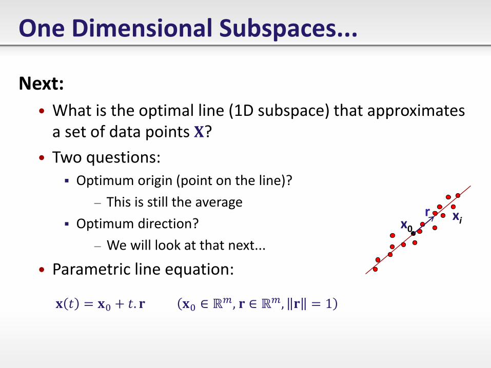
Next:
• What is the optimal line (1D subspace) that approximates a set of data points 𝐗?
• Two questions:
Optimum origin (point on the line)?
– This is still the average
Optimum direction?
– We will look at that next...
• Parametric line equation:
x0 xi
r
𝐱 𝑡 = 𝐱0 + 𝑡. 𝐫 𝐱0 ∈ ℝ𝑚, 𝐫 ∈ ℝ𝑚, 𝐫 = 1
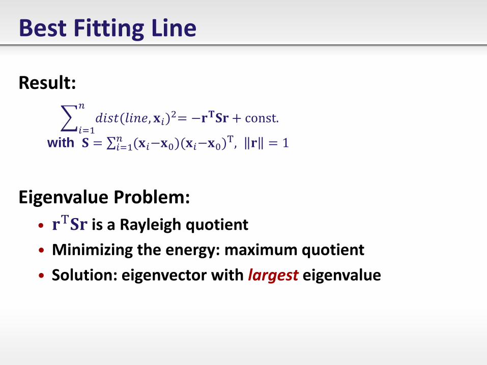
Best Fitting Line
Result:
Eigenvalue Problem:
• 𝐫T𝐒𝐫 is a Rayleigh quotient
• Minimizing the energy: maximum quotient
• Solution: eigenvector with largest eigenvalue
𝑑𝑖𝑠𝑡 𝑙𝑖𝑛𝑒, 𝐱𝑖 2= −𝐫𝐓𝐒𝐫
𝑛
𝑖=1+ const.
with 𝐒 = 𝐱𝑖−𝐱0 𝐱𝑖−𝐱0 T, 𝐫 = 1𝑛
𝑖=1
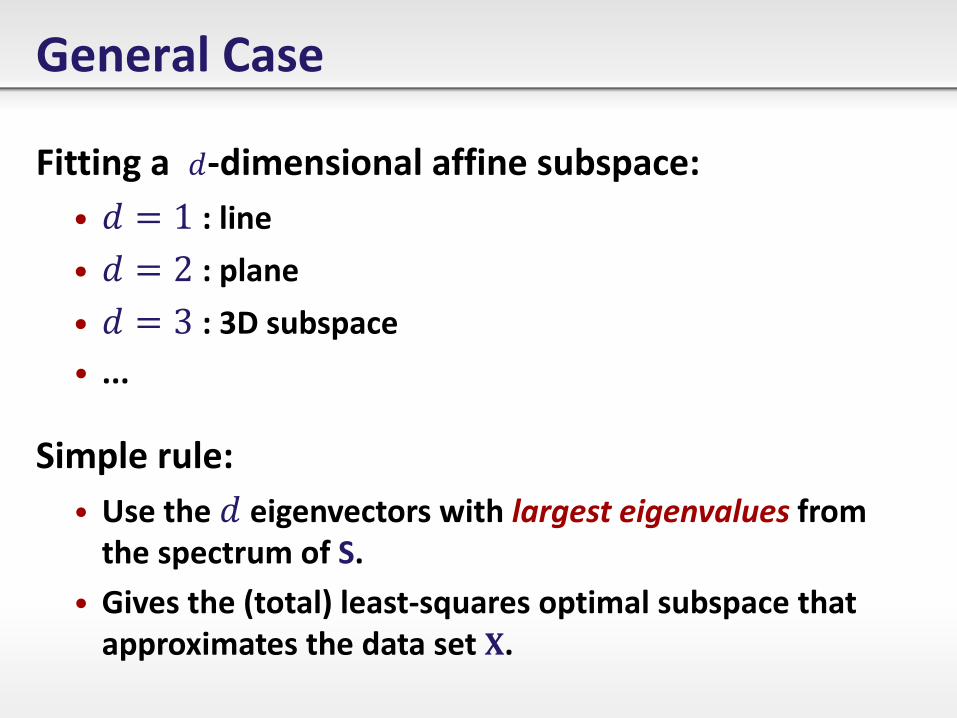
General Case
Fitting a 𝑑-dimensional affine subspace:
• 𝑑 = 1 : line
• 𝑑 = 2 : plane
• 𝑑 = 3 : 3D subspace
• ...
Simple rule:
• Use the 𝑑 eigenvectors with largest eigenvalues from the spectrum of S.
• Gives the (total) least-squares optimal subspace that approximates the data set 𝐗.
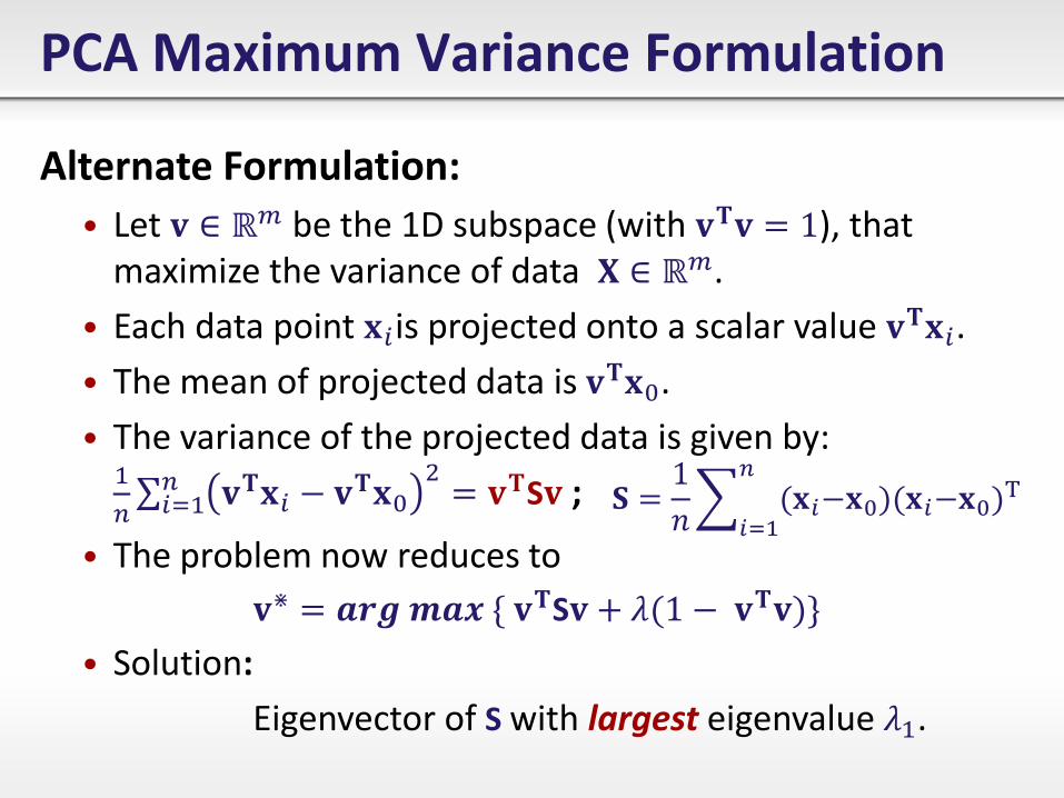
PCA Maximum Variance Formulation
Alternate Formulation:
• Let 𝐯 ∈ ℝ𝑚 be the 1D subspace (with 𝐯𝐓𝐯 = 1), that maximize the variance of data 𝐗 ∈ ℝ𝑚.
• Each data point 𝐱𝑖is projected onto a scalar value 𝐯𝐓𝐱𝑖.
• The mean of projected data is 𝐯𝐓𝐱0.
• The variance of the projected data is given by: 1
𝑛 𝐯𝐓𝐱𝑖 − 𝐯𝐓𝐱0
2𝑛𝑖=1 = 𝐯𝐓S𝐯 ;
• The problem now reduces to
𝐯⋇ = 𝒂𝒓𝒈 𝒎𝒂𝒙 { 𝐯𝐓S𝐯 + 𝜆 1 − 𝐯𝐓𝐯 }
• Solution:
Eigenvector of S with largest eigenvalue 𝜆1.
𝐒 =1
𝑛 𝐱𝑖−𝐱0 𝐱𝑖−𝐱0
T𝑛
𝑖=1

Statistical Interpretation
Observation:
•𝟏
𝒏−𝟏𝐒 is the covariance matrix of the data 𝐗.
• PCA can be interpreted as fitting a Gaussian distribution and computing the main axes.
x0
11 v
12 v
)(, xμΣN
𝛍 = 𝐱0 =1
𝑛 𝐱𝑖
𝑛
𝑖=1
𝚺 = 1
𝑛 − 1𝐒 =
1
𝑛 − 1 𝐱𝑖−𝐱0 𝐱𝑖−𝐱0
T
𝑛
𝑖=1
𝑁𝚺,𝛍 𝐱 =1
2𝜋𝑑2 det 𝚺 1/2
exp −1
2 𝐱 − 𝛍 T𝚺−1 𝐱 − 𝛍
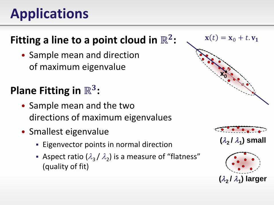
Applications
Fitting a line to a point cloud in ℝ𝟐:
• Sample mean and direction of maximum eigenvalue
Plane Fitting in ℝ𝟑:
• Sample mean and the two directions of maximum eigenvalues
• Smallest eigenvalue
Eigenvector points in normal direction
Aspect ratio (3 / 2) is a measure of “flatness” (quality of fit)
x0
(2 / 1) small
(2 / 1) larger
𝐱 𝑡 = 𝐱0 + 𝑡. 𝐯𝟏
Applications
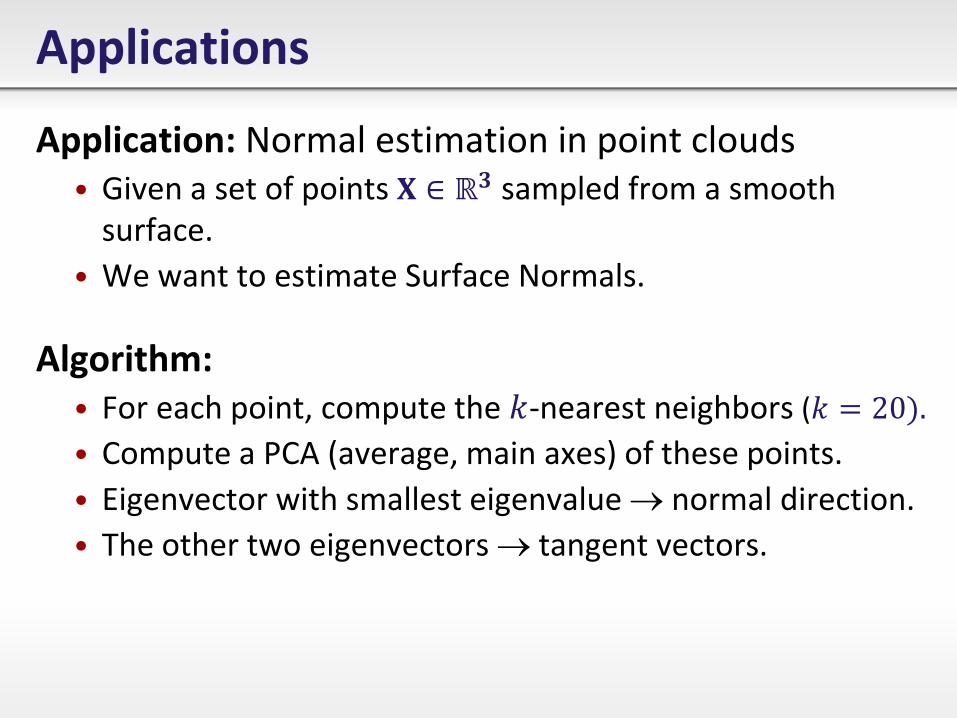
Application: Normal estimation in point clouds • Given a set of points 𝐗 ∈ ℝ𝟑 sampled from a smooth
surface.
• We want to estimate Surface Normals.
Algorithm: • For each point, compute the 𝑘-nearest neighbors (𝑘 = 20 .
• Compute a PCA (average, main axes) of these points.
• Eigenvector with smallest eigenvalue normal direction.
• The other two eigenvectors tangent vectors.
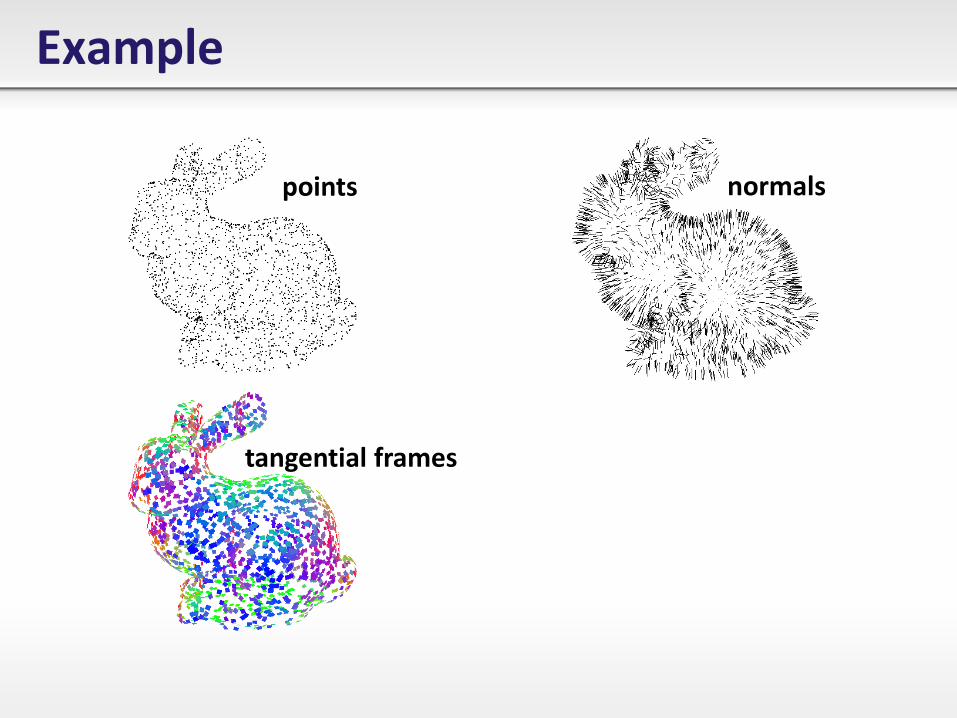
Example
points normals
tangential frames
Dimensionality Reduction
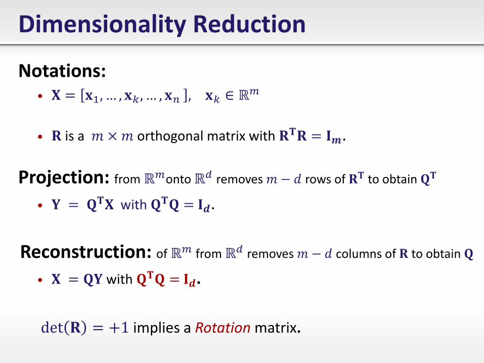
Notations: • 𝐗 = 𝐱1, … , 𝐱𝑘 , … , 𝐱𝑛 , 𝐱𝑘 ∈ ℝ𝑚
• 𝐑 is a 𝑚 ×𝑚 orthogonal matrix with 𝐑𝐓𝐑 = 𝐈𝒎.
Projection: from ℝ𝑚onto ℝ𝑑 removes 𝑚− 𝑑 rows of 𝐑𝐓 to obtain 𝐐𝐓
• 𝐘 = 𝐐𝐓𝐗 with 𝐐𝐓𝐐 = 𝐈𝒅.
Reconstruction: of ℝ𝑚 from ℝ𝑑 removes 𝑚− 𝑑 columns of 𝐑 to obtain 𝐐
• 𝐗 = 𝐐𝐘 with 𝐐𝐓𝐐 = 𝐈𝒅.
det 𝐑 = +1 implies a Rotation matrix.
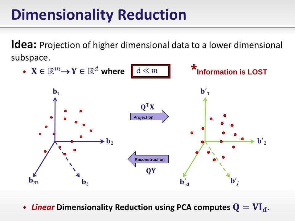
Idea: Projection of higher dimensional data to a lower dimensional
subspace.
• 𝐗 ∈ ℝ𝑚 𝐘 ∈ ℝ𝑑 where
𝐐𝐓𝐗
𝐐𝐘
• Linear Dimensionality Reduction using PCA computes 𝐐 = 𝐕𝐈𝒅.
Dimensionality Reduction
𝐛′1
𝐛′2
𝐛′𝑗 𝐛′𝑑
Projection
𝐛1
𝐛2
𝐛𝑖 𝐛𝑚
𝑑 ≪ 𝑚
Reconstruction
*Information is LOST
Metric Multi Dimensional Scaling
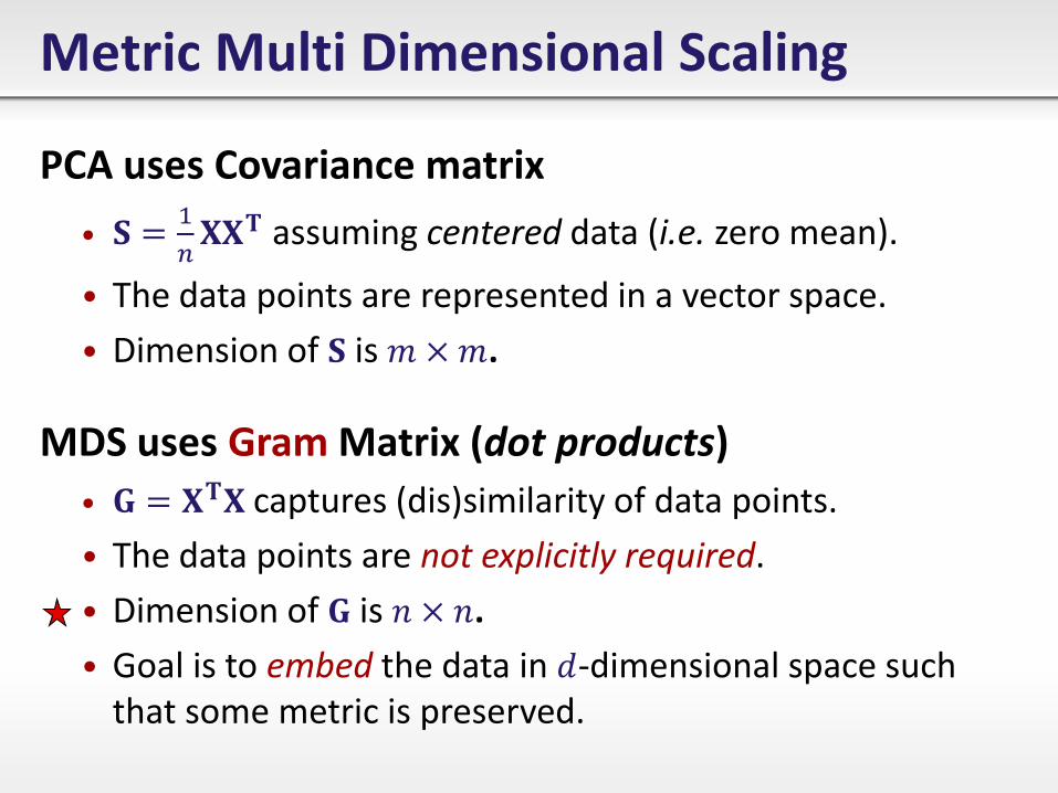
PCA uses Covariance matrix
• 𝐒 =1
𝑛𝐗𝐗𝐓 assuming centered data (i.e. zero mean).
• The data points are represented in a vector space.
• Dimension of 𝐒 is 𝑚 ×𝑚.
MDS uses Gram Matrix (dot products)
• 𝐆 = 𝐗𝐓𝐗 captures (dis)similarity of data points.
• The data points are not explicitly required.
• Dimension of 𝐆 is 𝑛 × 𝑛.
• Goal is to embed the data in 𝑑-dimensional space such that some metric is preserved.
Part III: Intrinsic Geometry and Intrinsic Mappings
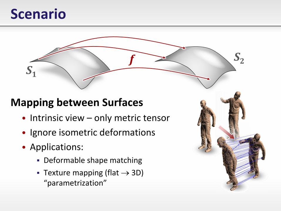
Scenario
Mapping between Surfaces
• Intrinsic view – only metric tensor
• Ignore isometric deformations
• Applications:
Deformable shape matching
Texture mapping (flat 3D) “parametrization”
f S1
S2
Differential Geometry Revisited
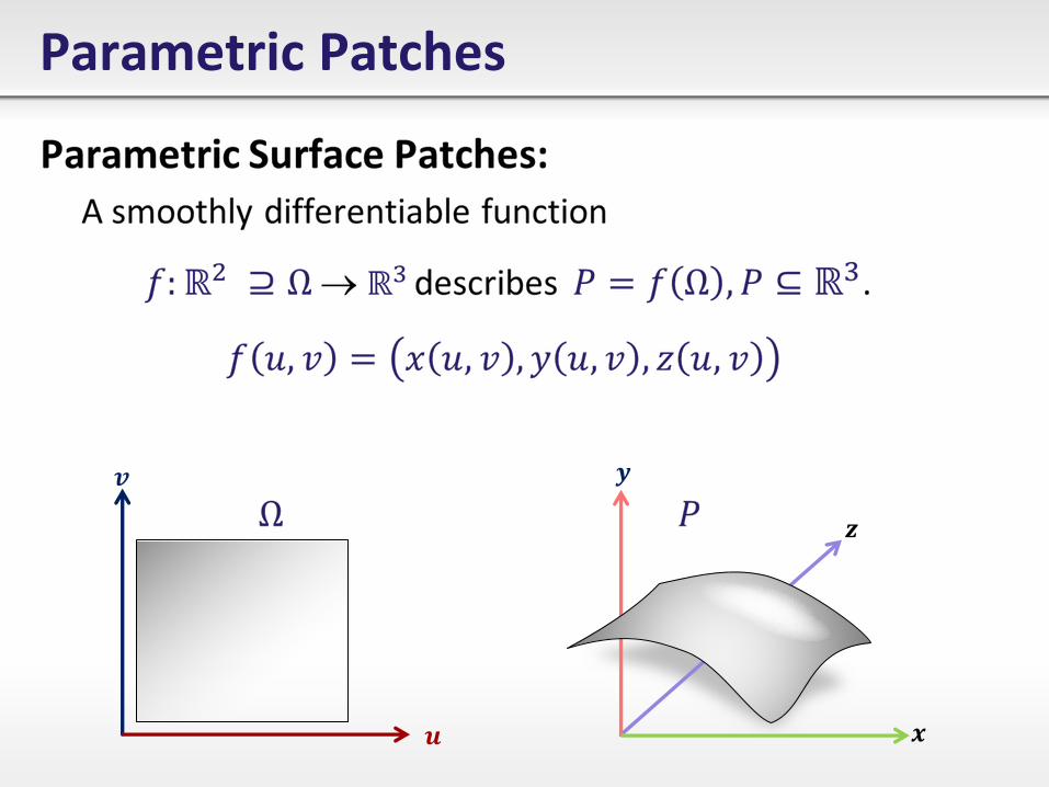
Parametric Patches
𝒖
𝒗 𝒚
𝒙
𝒛
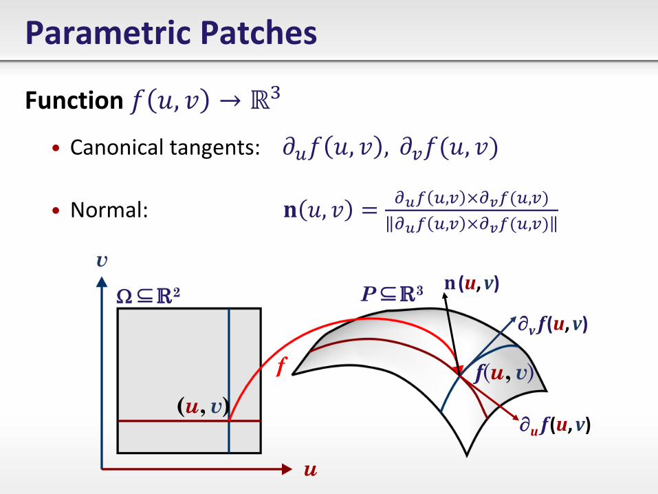
Parametric Patches
Function 𝑓 𝑢, 𝑣 → ℝ3
• Canonical tangents: 𝜕𝑢𝑓 𝑢, 𝑣 , 𝜕𝑣𝑓 𝑢, 𝑣
• Normal: 𝐧 𝑢, 𝑣 =𝜕𝑢𝑓 𝑢,𝑣 ×𝜕𝑣𝑓 𝑢,𝑣
𝜕𝑢𝑓 𝑢,𝑣 ×𝜕𝑣𝑓 𝑢,𝑣
u
v
(u, v)
f(u, v) f
2 P 3
v f (u, v)
u f (u, v)
n (u, v)
Fundamental Forms
Fundamental Forms:
• Describe the local parameterized surface.
• Measure...
...distortion of length (first fundamental form)
...surface curvature (second fundamental form)
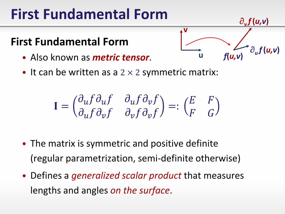
First Fundamental Form
First Fundamental Form
• Also known as metric tensor.
• It can be written as a 2 × 2 symmetric matrix:
𝐈 =𝜕𝑢𝑓𝜕𝑢𝑓 𝜕𝑢𝑓𝜕𝑣𝑓𝜕𝑢𝑓𝜕𝑣𝑓 𝜕𝑣𝑓𝜕𝑣𝑓
=: 𝐸 𝐹𝐹 𝐺
• The matrix is symmetric and positive definite
(regular parametrization, semi-definite otherwise)
• Defines a generalized scalar product that measures
lengths and angles on the surface.
v
u
v f (u,v)
u f (u,v) f(u,v)
Second Fundamental Form
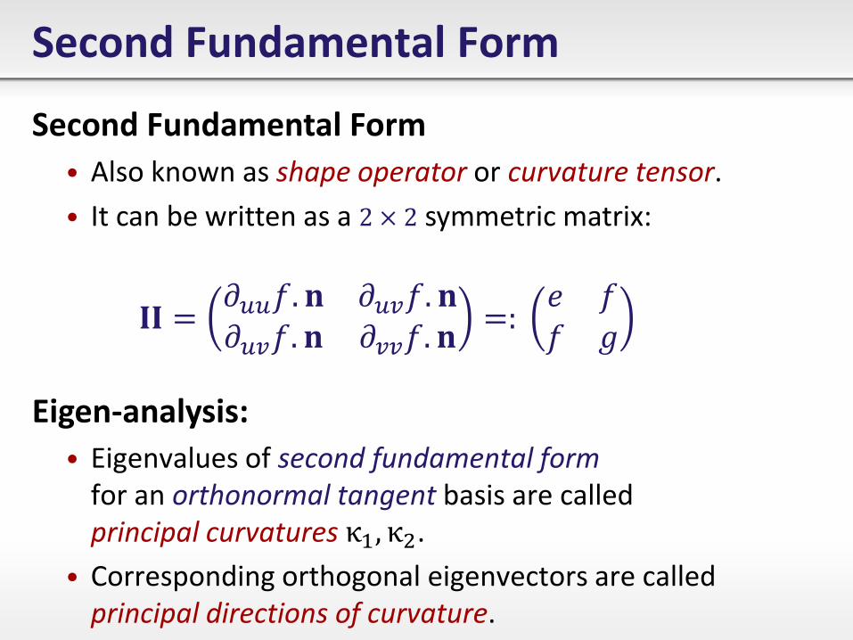
Second Fundamental Form
• Also known as shape operator or curvature tensor.
• It can be written as a 2 × 2 symmetric matrix:
𝐈𝐈 =𝜕𝑢𝑢𝑓. 𝐧 𝜕𝑢𝑣𝑓. 𝐧𝜕𝑢𝑣𝑓. 𝐧 𝜕𝑣𝑣𝑓. 𝐧
=: 𝑒 𝑓𝑓 𝑔
Eigen-analysis:
• Eigenvalues of second fundamental form for an orthonormal tangent basis are called principal curvatures κ1, κ2.
• Corresponding orthogonal eigenvectors are called principal directions of curvature.
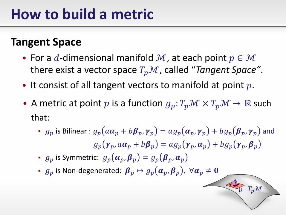
• A metric at point 𝑝 is a function 𝑔𝑝: 𝑇𝑝ℳ×𝑇𝑝ℳ→ ℝ such
that:
𝑔𝑝 is Bilinear : 𝑔𝑝 𝑎𝜶𝑝 + 𝑏𝜷𝑝, 𝜸𝑝 = 𝑎𝑔𝑝 𝜶𝑝, 𝜸𝑝 + 𝑏𝑔𝑝 𝜷𝑝, 𝜸𝑝 and
𝑔𝑝 𝜸𝑝, 𝑎𝜶𝑝 + 𝑏𝜷𝑝 = 𝑎𝑔𝑝 𝜸𝑝, 𝜶𝑝 + 𝑏𝑔𝑝 𝜸𝑝, 𝜷𝑝
𝑔𝑝 is Symmetric: 𝑔𝑝 𝜶𝑝, 𝜷𝑝 = 𝑔𝑝 𝜷𝑝, 𝜶𝑝
𝑔𝑝 is Non-degenerated: 𝜷𝑝 ↦ 𝑔𝑝 𝜶𝑝, 𝜷𝑝 , ∀𝜶𝑝 ≠ 𝟎
How to build a metric
Tangent Space
• For a 𝑑-dimensional manifold ℳ, at each point 𝑝 ∈ ℳ there exist a vector space 𝑇𝑝ℳ, called “Tangent Space”.
• It consist of all tangent vectors to manifold at point 𝑝.
𝑇𝑝ℳ 𝑝
How to build a metric
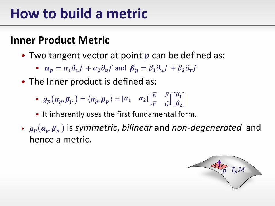
Inner Product Metric
• Two tangent vector at point 𝑝 can be defined as: 𝜶𝒑 = 𝛼1𝜕𝑢𝑓 + 𝛼2𝜕𝒗𝑓 and 𝜷𝒑 = 𝛽1𝜕𝑢𝑓 + 𝛽2𝜕𝒗𝑓
• The Inner product is defined as:
𝑔𝑝 𝜶𝒑, 𝜷𝒑 = 𝜶𝒑, 𝜷𝒑 = 𝛼1 𝛼2𝐸 𝐹
𝐹 𝐺
𝛽1𝛽2
It inherently uses the first fundamental form.
• 𝑔𝑝 𝜶𝒑, 𝜷𝒑 is symmetric, bilinear and non-degenerated and hence a metric.
𝑇𝑝ℳ 𝑝
Riemannian Manifolds
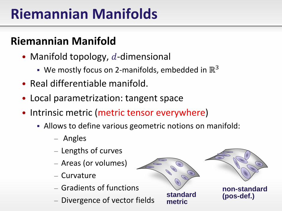
Riemannian Manifold
• Manifold topology, 𝑑-dimensional
We mostly focus on 2-manifolds, embedded in ℝ3
• Real differentiable manifold.
• Local parametrization: tangent space
• Intrinsic metric (metric tensor everywhere)
Allows to define various geometric notions on manifold:
– Angles
– Lengths of curves
– Areas (or volumes)
– Curvature
– Gradients of functions
– Divergence of vector fields standard metric
non-standard (pos-def.)
Riemannian Manifolds
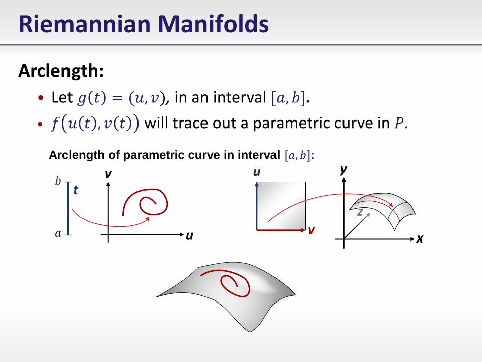
Arclength:
• Let 𝑔 𝑡 = 𝑢, 𝑣 , in an interval [𝑎, 𝑏].
• 𝑓 𝑢 𝑡 , 𝑣 𝑡 will trace out a parametric curve in 𝑃.
Arclength of parametric curve in interval [𝑎, 𝑏]:
u
v x
y
z
t v
u
𝑏
𝑎
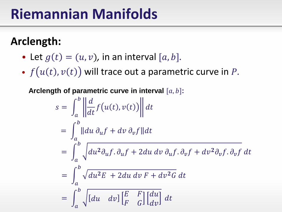
= 𝑑𝑢𝟐𝐸 + 2𝑑𝑢 𝑑𝑣 𝐹 + 𝑑𝑣𝟐𝐺 𝑑𝑡𝑏
𝑎
Riemannian Manifolds
Arclength:
• Let 𝑔 𝑡 = 𝑢, 𝑣 , in an interval [𝑎, 𝑏].
• 𝑓 𝑢 𝑡 , 𝑣 𝑡 will trace out a parametric curve in 𝑃.
= 𝑑𝑢𝟐𝜕𝑢𝑓. 𝜕𝑢𝑓 + 2𝑑𝑢 𝑑𝑣 𝜕𝑢𝑓. 𝜕𝑣𝑓 + 𝑑𝑣𝟐𝜕𝑣𝑓. 𝜕𝑣𝑓 𝑑𝑡𝑏
𝑎
𝑠 = 𝑑
𝑑𝑡𝑓 𝑢 𝑡 , 𝑣 𝑡 𝑑𝑡
𝑏
𝑎
= 𝑑𝑢 𝜕𝑢𝑓 + 𝑑𝑣 𝜕𝑣𝑓 𝑑𝑡
𝑏
𝑎
Arclength of parametric curve in interval [𝑎, 𝑏]:
= 𝑑𝑢 𝑑𝑣𝐸 𝐹𝐹 𝐺
𝑑𝑢𝑑𝑣
𝑑𝑡𝑏
𝑎
Riemannian Manifolds
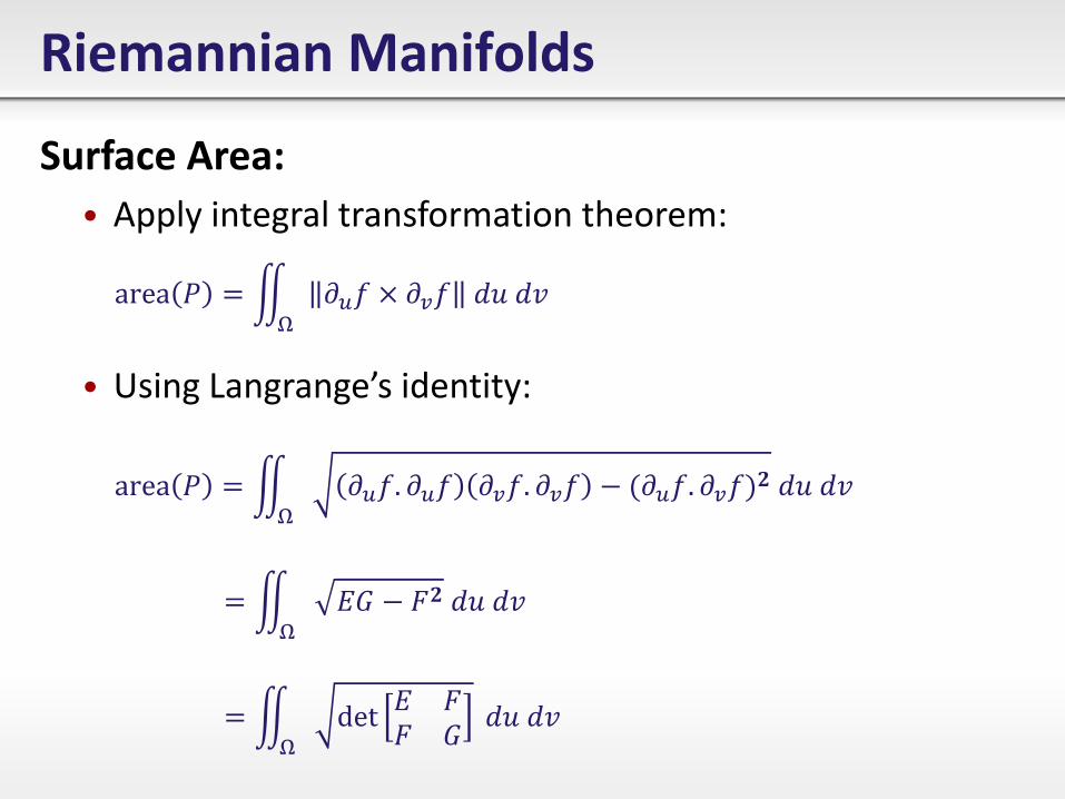
Surface Area:
• Apply integral transformation theorem:
• Using Langrange’s identity:
area 𝑃 = 𝜕𝑢𝑓. 𝜕𝑢𝑓 𝜕𝑣𝑓. 𝜕𝑣𝑓 − 𝜕𝑢𝑓. 𝜕𝑣𝑓 𝟐 𝑑𝑢 𝑑𝑣
Ω
= 𝐸𝐺 − 𝐹𝟐 𝑑𝑢 𝑑𝑣Ω
= det𝐸 𝐹𝐹 𝐺
𝑑𝑢 𝑑𝑣Ω
area 𝑃 = 𝜕𝑢𝑓 × 𝜕𝑣𝑓 𝑑𝑢 𝑑𝑣Ω
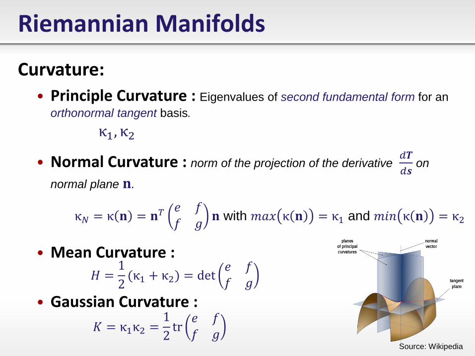
Curvature:
• Principle Curvature : Eigenvalues of second fundamental form for an
orthonormal tangent basis.
• Normal Curvature : norm of the projection of the derivative 𝑑𝑻
𝑑𝒔 on
normal plane 𝐧.
• Mean Curvature :
• Gaussian Curvature :
Riemannian Manifolds
κ1, κ2
κ𝑁 = κ 𝐧 = 𝐧𝑇𝑒 𝑓𝑓 𝑔
𝐧 with 𝑚𝑎𝑥 κ 𝐧 = κ1 and 𝑚𝑖𝑛 κ 𝐧 = κ2
𝐻 =1
2 κ1 + κ2 = det
𝑒 𝑓𝑓 𝑔
𝐾 = κ1κ2 =1
2tr
𝑒 𝑓𝑓 𝑔
Source: Wikipedia
Riemannian Manifolds
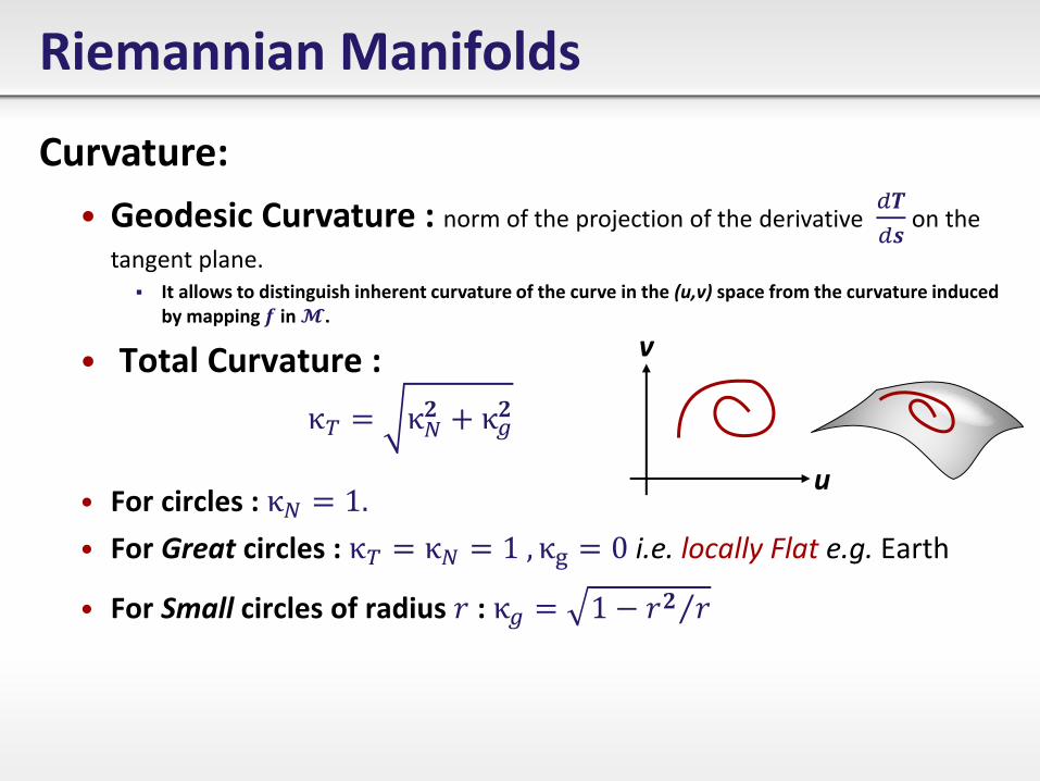
Curvature:
• Geodesic Curvature : norm of the projection of the derivative 𝑑𝑻
𝑑𝒔 on the
tangent plane. It allows to distinguish inherent curvature of the curve in the (u,v) space from the curvature induced
by mapping 𝒇 in 𝓜.
• Total Curvature :
• For circles : κ𝑁 = 1.
• For Great circles : κ𝑇 = κ𝑁 = 1 , κg = 0 i.e. locally Flat e.g. Earth
• For Small circles of radius 𝑟 : κ𝑔 = 1 − 𝑟𝟐 𝑟
κ𝑇 = κ𝑁𝟐 + κ𝑔
𝟐
v
u
Riemannian Manifolds
35
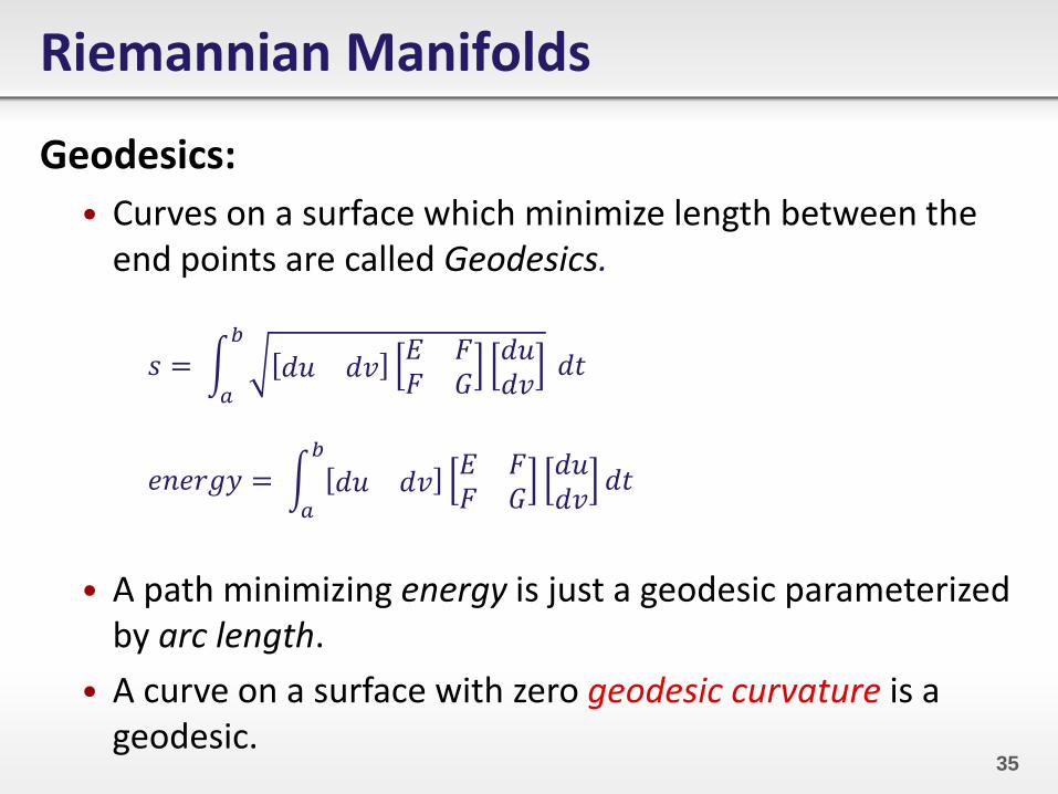
Geodesics:
• Curves on a surface which minimize length between the end points are called Geodesics.
• A path minimizing energy is just a geodesic parameterized by arc length.
• A curve on a surface with zero geodesic curvature is a geodesic.
𝑠 = 𝑑𝑢 𝑑𝑣𝐸 𝐹𝐹 𝐺
𝑑𝑢𝑑𝑣
𝑑𝑡𝑏
𝑎
𝑒𝑛𝑒𝑟𝑔𝑦 = 𝑑𝑢 𝑑𝑣𝐸 𝐹𝐹 𝐺
𝑑𝑢𝑑𝑣
𝑑𝑡𝑏
𝑎
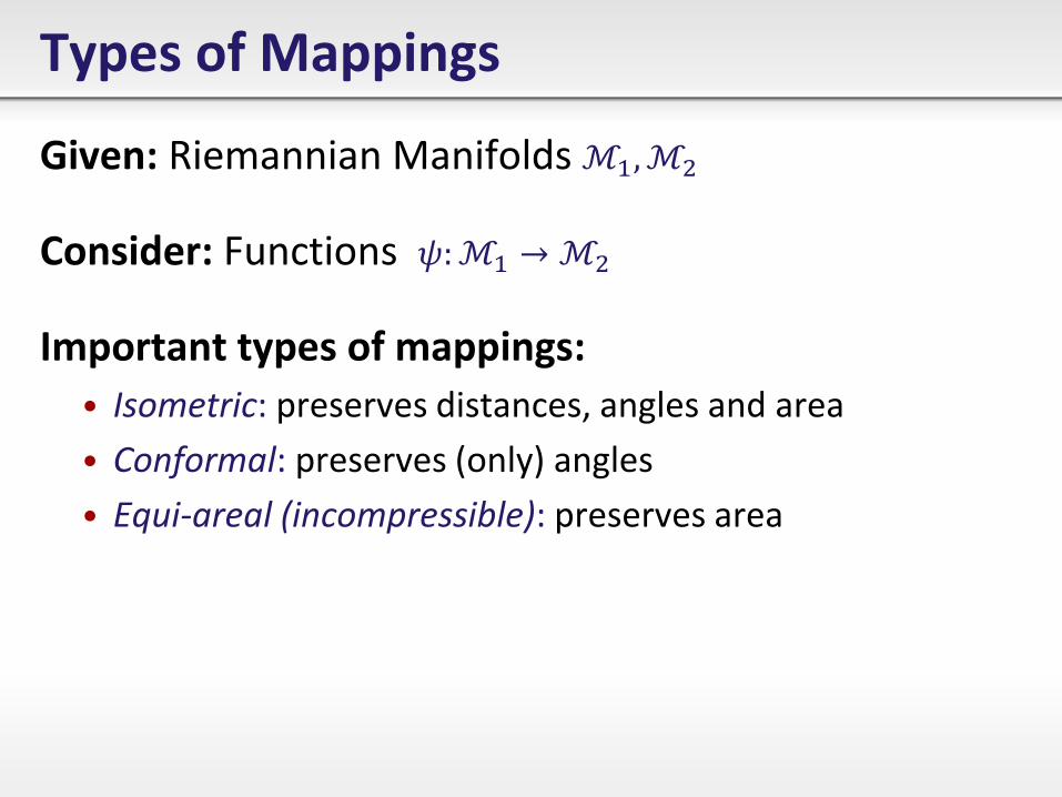
Types of Mappings
Given: Riemannian Manifolds ℳ1,ℳ2
Consider: Functions 𝜓:ℳ1 →ℳ2
Important types of mappings:
• Isometric: preserves distances, angles and area
• Conformal: preserves (only) angles
• Equi-areal (incompressible): preserves area
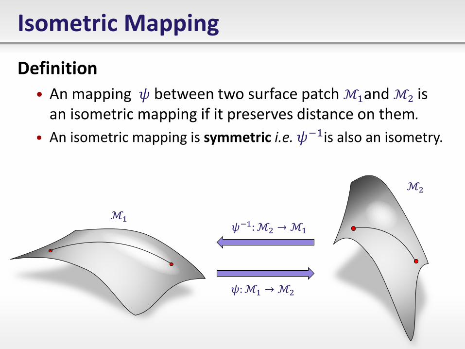
Isometric Mapping
Definition
• An mapping 𝜓 between two surface patch ℳ1and ℳ2 is an isometric mapping if it preserves distance on them.
• An isometric mapping is symmetric i.e. 𝜓−1is also an isometry.
ℳ1
ℳ2
𝜓:ℳ1 →ℳ2
𝜓−1:ℳ2 →ℳ1
Isometric Mapping
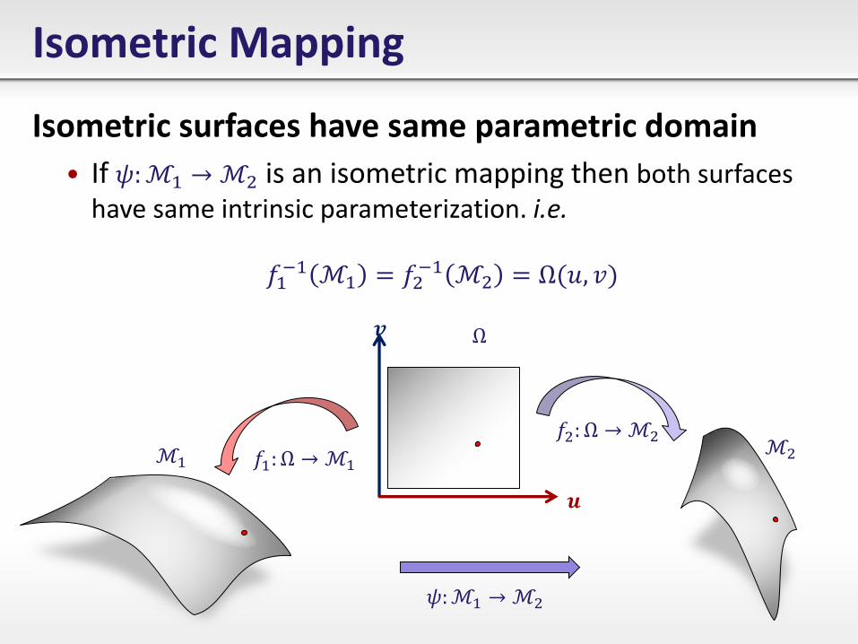
Isometric surfaces have same parametric domain
• If 𝜓:ℳ1 →ℳ2 is an isometric mapping then both surfaces have same intrinsic parameterization. i.e.
𝑓1−1 ℳ1 = 𝑓2
−1 ℳ2 = Ω 𝑢, 𝑣
𝒖
𝒗 Ω
ℳ1 ℳ2
𝜓:ℳ1 →ℳ2
𝑓2: Ω → ℳ2
𝑓1: Ω → ℳ1
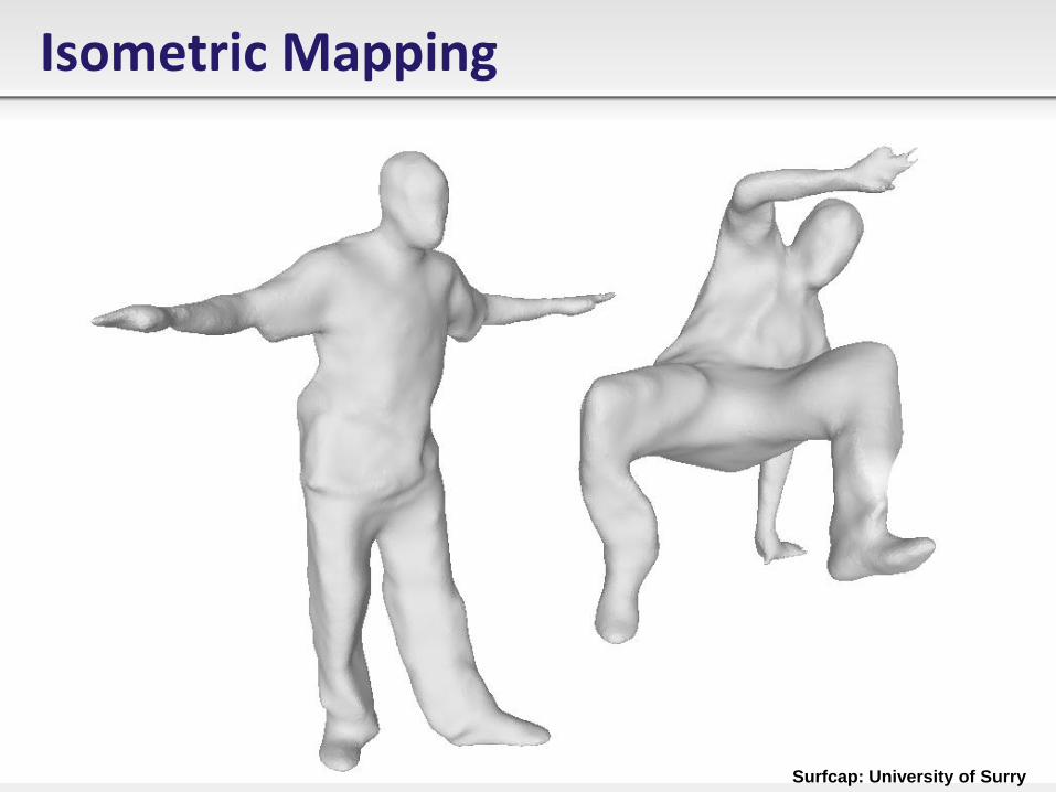
Isometric Mapping
Surfcap: University of Surry
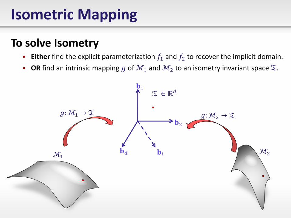
Isometric Mapping
To solve Isometry • Either find the explicit parameterization 𝑓1 and 𝑓2 to recover the implicit domain.
• OR find an intrinsic mapping 𝑔 of ℳ1 and ℳ2 to an isometry invariant space 𝔗.
ℳ1 ℳ2
𝐛1
𝐛2
𝐛𝑖 𝐛𝑑
𝑔:ℳ1 → 𝔗 𝑔:ℳ2 → 𝔗
𝔗 ∈ ℝ𝑑
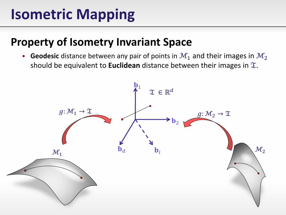
Isometric Mapping
Property of Isometry Invariant Space • Geodesic distance between any pair of points in ℳ1 and their images in ℳ2
should be equivalent to Euclidean distance between their images in 𝔗.
ℳ1 ℳ2
𝐛1
𝐛2
𝐛𝑖 𝐛𝑑
𝑔:ℳ1 → 𝔗 𝑔:ℳ2 → 𝔗
𝔗 ∈ ℝ𝑑
Spectral Graph Methods for 3D Shape Analysis
Discrete Manifold Representation
𝒚
𝒙
𝒛
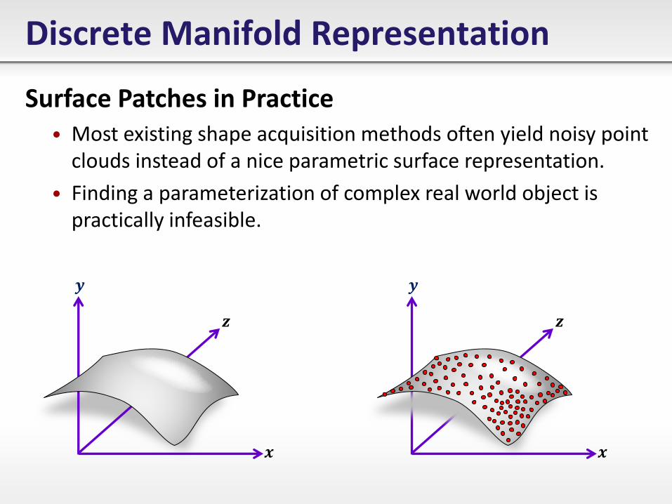
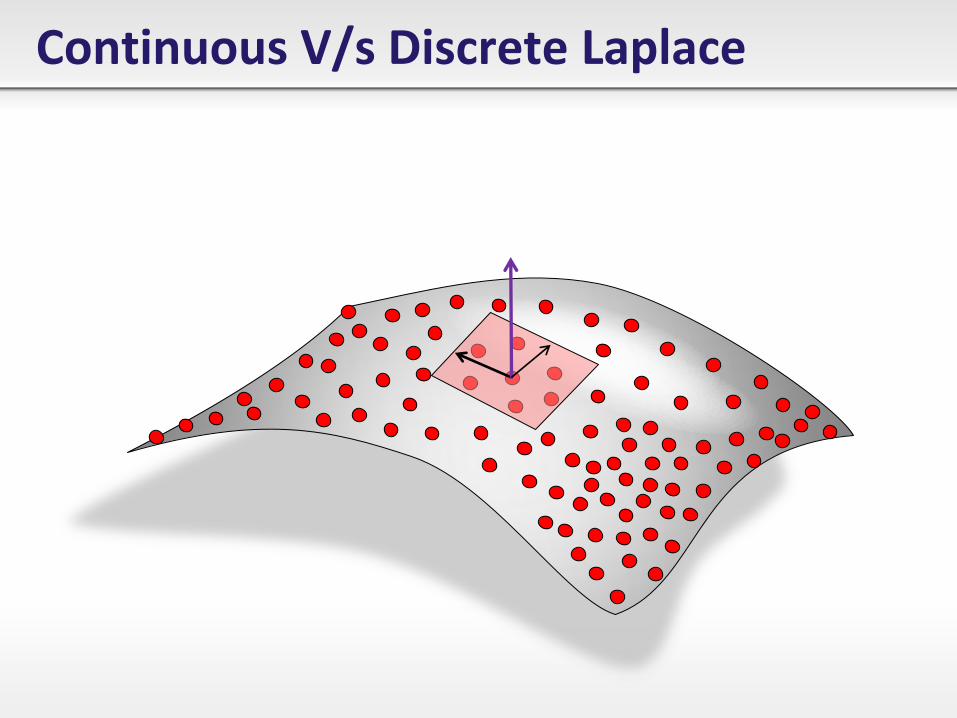
Surface Patches in Practice • Most existing shape acquisition methods often yield noisy point
clouds instead of a nice parametric surface representation.
• Finding a parameterization of complex real world object is practically infeasible.
𝒙
𝒚
𝒛
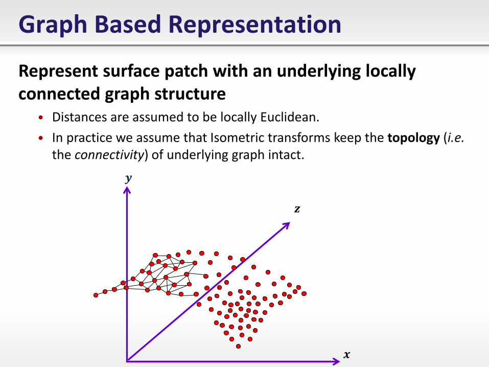
Represent surface patch with an underlying locally connected graph structure
• Distances are assumed to be locally Euclidean.
• In practice we assume that Isometric transforms keep the topology (i.e. the connectivity) of underlying graph intact.
Graph Based Representation
𝒚
𝒙
𝒛
Graph Based Representation
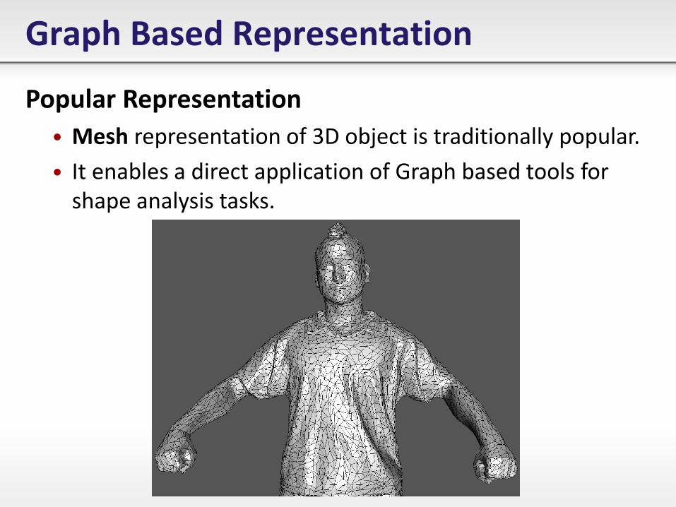
Popular Representation
• Mesh representation of 3D object is traditionally popular.
• It enables a direct application of Graph based tools for shape analysis tasks.
Spectral Graph Theory (SGT)
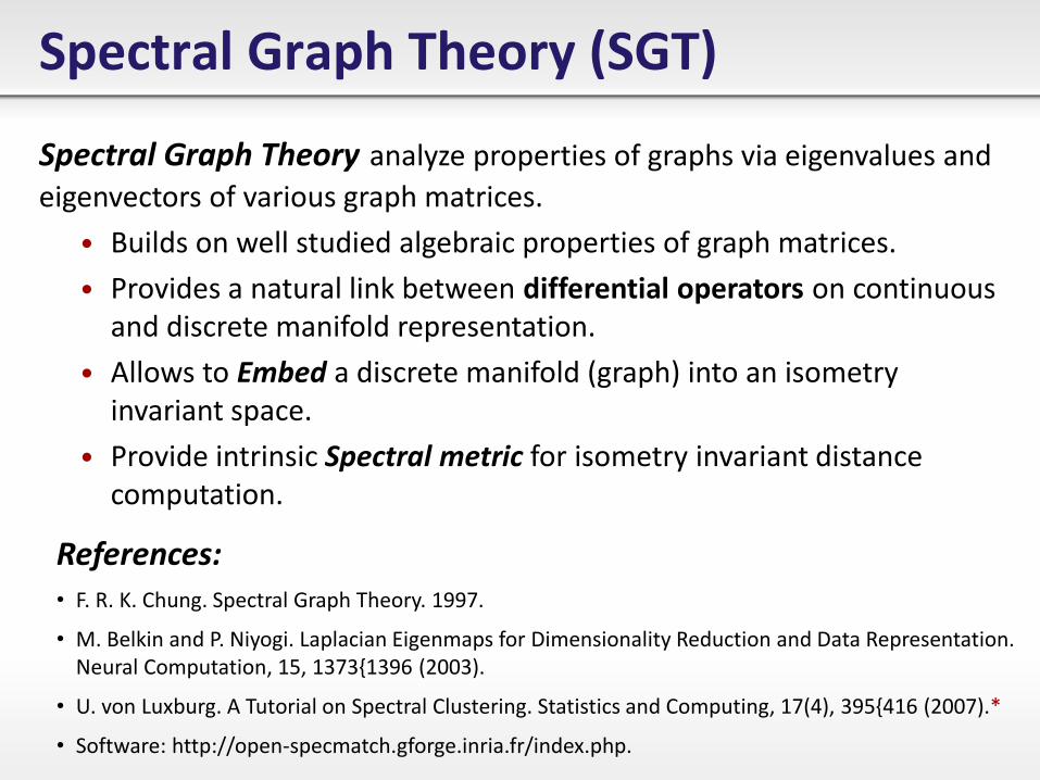
Spectral Graph Theory analyze properties of graphs via eigenvalues and
eigenvectors of various graph matrices.
• Builds on well studied algebraic properties of graph matrices.
• Provides a natural link between differential operators on continuous and discrete manifold representation.
• Allows to Embed a discrete manifold (graph) into an isometry invariant space.
• Provide intrinsic Spectral metric for isometry invariant distance computation.
References: • F. R. K. Chung. Spectral Graph Theory. 1997.
• M. Belkin and P. Niyogi. Laplacian Eigenmaps for Dimensionality Reduction and Data Representation. Neural Computation, 15, 1373{1396 (2003).
• U. von Luxburg. A Tutorial on Spectral Clustering. Statistics and Computing, 17(4), 395{416 (2007).*
• Software: http://open-specmatch.gforge.inria.fr/index.php.
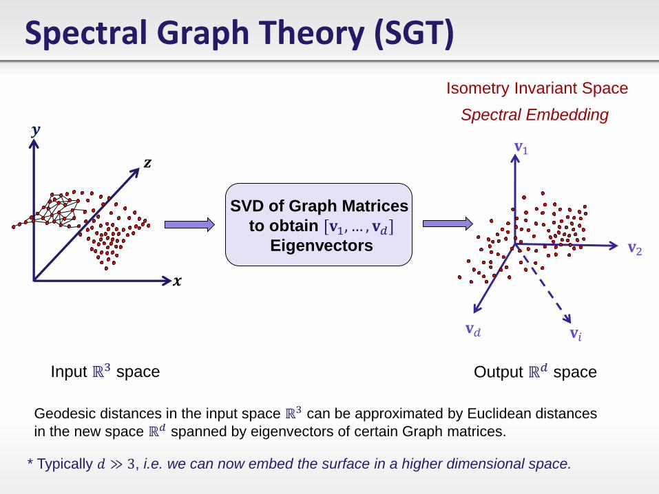
Spectral Graph Theory (SGT)
𝒚
𝒙
𝒛 𝐯1
𝐯2
𝐯𝑖 𝐯𝑑
SVD of Graph Matrices
to obtain [𝐯1, … , 𝐯𝑑] Eigenvectors
Input ℝ3 space Output ℝ𝑑 space
Isometry Invariant Space
Spectral Embedding
* Typically 𝑑 ≫ 3, i.e. we can now embed the surface in a higher dimensional space.
Geodesic distances in the input space ℝ3 can be approximated by Euclidean distances
in the new space ℝ𝑑 spanned by eigenvectors of certain Graph matrices.
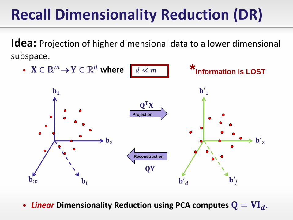
Idea: Projection of higher dimensional data to a lower dimensional
subspace.
• 𝐗 ∈ ℝ𝑚 𝐘 ∈ ℝ𝑑 where
𝐐𝐓𝐗
𝐐𝐘
• Linear Dimensionality Reduction using PCA computes 𝐐 = 𝐕𝐈𝒅.
Recall Dimensionality Reduction (DR)
𝐛′1
𝐛′2
𝐛′𝑗 𝐛′𝑑
Projection
𝐛1
𝐛2
𝐛𝑖 𝐛𝑚
𝑑 ≪ 𝑚
Reconstruction
*Information is LOST
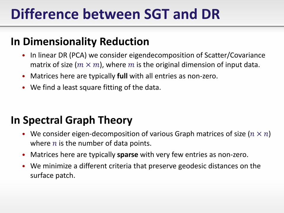
In Spectral Graph Theory • We consider eigen-decomposition of various Graph matrices of size (𝑛 × 𝑛)
where 𝑛 is the number of data points.
• Matrices here are typically sparse with very few entries as non-zero.
• We minimize a different criteria that preserve geodesic distances on the surface patch.
Difference between SGT and DR
In Dimensionality Reduction • In linear DR (PCA) we consider eigendecomposition of Scatter/Covariance
matrix of size (𝑚 ×𝑚), where 𝑚 is the original dimension of input data.
• Matrices here are typically full with all entries as non-zero.
• We find a least square fitting of the data.
Graph Matrices
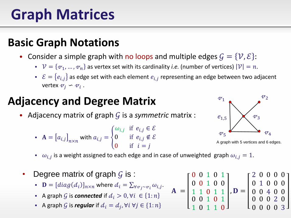
Basic Graph Notations • Consider a simple graph with no loops and multiple edges 𝒢 = 𝒱, ℰ :
𝒱 = 𝓋1, … , 𝓋𝑛 as vertex set with its cardinality i.e. (number of vertices) 𝒱 = 𝑛.
ℰ = 𝑒𝑖,𝑗 as edge set with each element 𝑒𝑖,𝑗 representing an edge between two adjacent
vertex 𝓋𝑗 ∽ 𝓋𝑖 .
Adjacency and Degree Matrix • Adjacency matrix of graph 𝒢 is a symmetric matrix :
𝐀 = 𝑎𝑖,𝑗 𝑛×𝑛 with 𝑎𝑖,𝑗 =
𝜔𝑖,𝑗 if 𝑒𝑖,𝑗 ∈ ℰ
0 if 𝑒𝑖,𝑗 ∉ ℰ
0 if 𝑖 = 𝑗
𝜔𝑖,𝑗 is a weight assigned to each edge and in case of unweighted graph 𝜔𝑖,𝑗 = 1.
• Degree matrix of graph 𝒢 is :
𝐃 = [𝑑𝑖𝑎𝑔 𝒹𝑖 ]𝑛×𝑛 where 𝒹𝑖 = 𝜔𝑖,𝑗∀𝓋𝑗~𝓋𝑖.
A graph 𝒢 is connected if 𝒹𝑖 > 0, ∀𝑖 ∈ 1: 𝑛
A graph 𝒢 is regular if 𝒹𝑖 = 𝒹𝑗 , ∀𝑖 ∀𝑗 ∈ {1: 𝑛}
𝓋1 𝓋2
𝓋3
𝓋4 𝓋5
𝑒1,5
A graph with 5 vertices and 6 edges.
𝐀 =
0 0 1
0 0 1
1 1 0
0 0 1
1 0 1
0 1 0 0 1 1 0 1 1 0
, 𝐃 =
2 0 0
0 1 0
0 0 4
0 0 0
0 0 0
0 0 0 0 0 0 2 0 0 3
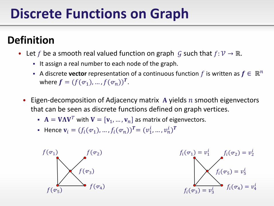
• Eigen-decomposition of Adjacency matrix 𝐀 yields 𝑛 smooth eigenvectors that can be seen as discrete functions defined on graph vertices.
𝐀 = 𝐕𝚲𝐕𝑇 with 𝐕 = [𝐯1, … , 𝐯𝑛] as matrix of eigenvectors.
Hence 𝐯𝑖 = 𝑓𝑖 𝓋1 , … , 𝑓𝑖 𝓋𝑛 𝑻= 𝑣1
𝑖 , … , 𝑣𝑛𝑖 𝑻
Discrete Functions on Graph
Definition • Let 𝑓 be a smooth real valued function on graph 𝒢 such that 𝑓:𝒱 → ℝ.
It assign a real number to each node of the graph.
A discrete vector representation of a continuous function 𝑓 is written as 𝒇 ∈ ℝ𝑛 where 𝒇 = 𝑓 𝓋1 , … , 𝑓 𝓋𝑛
𝑻.
𝑓 𝓋1 𝑓 𝓋2
𝑓 𝓋3
𝑓 𝓋4 𝑓 𝓋5
𝑓𝑖 𝓋1 = 𝑣1𝑖 𝑓𝑖 𝓋2 = 𝑣2
𝑖
𝑓𝑖 𝓋5 = 𝑣5𝑖
𝑓𝑖 𝓋4 = 𝑣4𝑖
𝑓𝑖 𝓋3 = 𝑣3𝑖
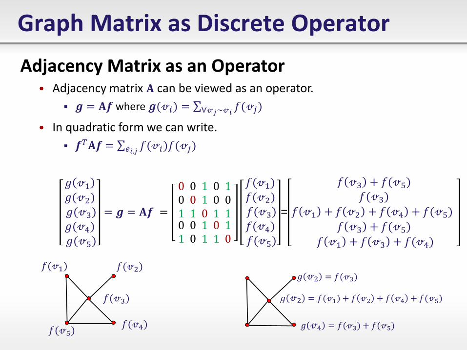
Graph Matrix as Discrete Operator
Adjacency Matrix as an Operator • Adjacency matrix 𝐀 can be viewed as an operator.
𝒈 = 𝐀𝒇 where 𝒈 𝓋𝑖 = 𝑓 𝓋𝑗 ∀𝓋𝑗~𝓋𝑖
• In quadratic form we can write.
𝒇𝑇𝐀𝒇 = 𝑓 𝓋𝑖 𝑓 𝓋𝑗 𝑒𝑖,𝑗
𝑔 𝓋1𝑔 𝓋2 𝑔 𝓋3 𝑔 𝓋4 𝑔 𝓋5
= 𝒈 = 𝐀𝒇 =
0 0 1
0 0 1
1 1 0
0 0 1
1 0 1
0 1 0 0 1 1 0 1 1 0
𝑓 𝓋1 𝑓 𝓋2 𝑓 𝓋3 𝑓 𝓋4 𝑓 𝓋5
=
𝑓 𝓋3 + 𝑓 𝓋5 𝑓 𝓋3
𝑓 𝓋1 + 𝑓 𝓋2 + 𝑓 𝓋4 + 𝑓 𝓋5 𝑓 𝓋3 + 𝑓 𝓋5
𝑓 𝓋1 + 𝑓 𝓋3 + 𝑓 𝓋4
𝑓 𝓋1 𝑓 𝓋2
𝑓 𝓋3
𝑓 𝓋4 𝑓 𝓋5 𝑔 𝓋4 = 𝑓 𝓋3 + 𝑓 𝓋5
𝑔 𝓋2 = 𝑓 𝓋3
𝑔 𝓋2 = 𝑓 𝓋1 + 𝑓 𝓋2 + 𝑓 𝓋4 + 𝑓 𝓋5
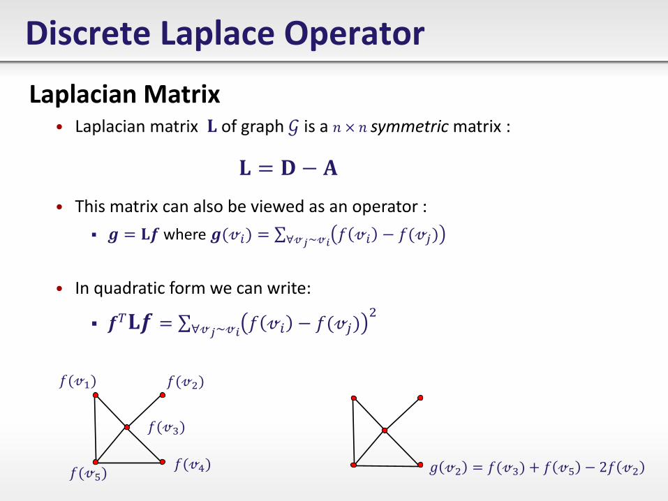
Discrete Laplace Operator
Laplacian Matrix • Laplacian matrix 𝐋 of graph 𝒢 is a 𝑛 × 𝑛 symmetric matrix :
• This matrix can also be viewed as an operator :
𝒈 = 𝐋𝒇 where 𝒈 𝓋𝑖 = 𝑓 𝓋𝑖 − 𝑓 𝓋𝑗 ∀𝓋𝑗~𝓋𝑖
• In quadratic form we can write:
𝒇𝑇𝐋𝒇 = 𝑓 𝓋𝑖 − 𝑓 𝓋𝑗 2
∀𝓋𝑗~𝓋𝑖
𝐋 = 𝐃 − 𝐀
𝑓 𝓋1 𝑓 𝓋2
𝑓 𝓋3
𝑓 𝓋4 𝑓 𝓋5 𝑔 𝓋2 = 𝑓 𝓋3 + 𝑓 𝓋5 − 2𝑓 𝓋2
Continuous V/s Discrete Laplace
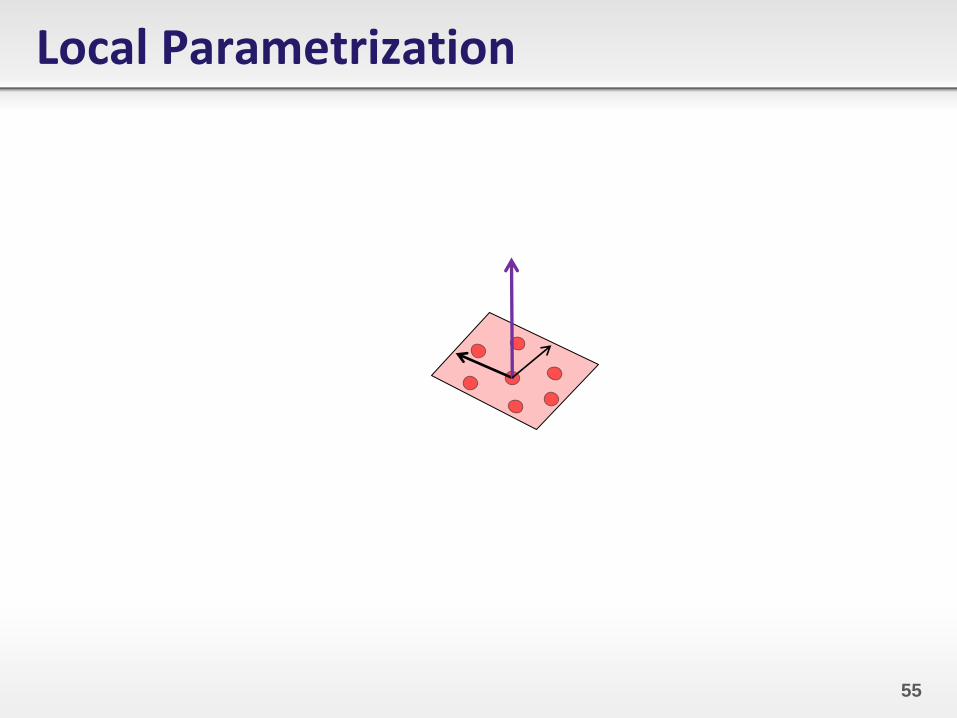
Local Parametrization
55
Continuous V/s Discrete Laplace
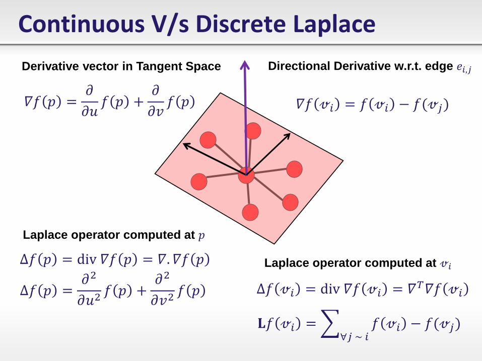
𝛻𝑓 𝑝 =𝜕
𝜕𝑢𝑓 𝑝 +
𝜕
𝜕𝑣𝑓 𝑝 𝛻𝑓 𝓋𝑖 = 𝑓 𝓋𝑖 − 𝑓 𝓋𝑗
Derivative vector in Tangent Space Directional Derivative w.r.t. edge 𝑒𝑖,𝑗
∆𝑓 𝑝 = div 𝛻𝑓 𝑝 = 𝛻. 𝛻𝑓 𝑝
∆𝑓 𝑝 =𝜕2
𝜕𝑢2𝑓 𝑝 +
𝜕2
𝜕𝑣2𝑓 𝑝
Laplace operator computed at 𝑝
Laplace operator computed at 𝓋𝑖
∆𝑓 𝓋𝑖 = div 𝛻𝑓 𝓋𝑖 = 𝛻𝑇𝛻𝑓 𝓋𝑖
𝐋𝑓 𝓋𝑖 = 𝑓 𝓋𝑖 − 𝑓 𝓋𝑗 ∀𝑗 ~ 𝑖
Discrete Laplace Operator
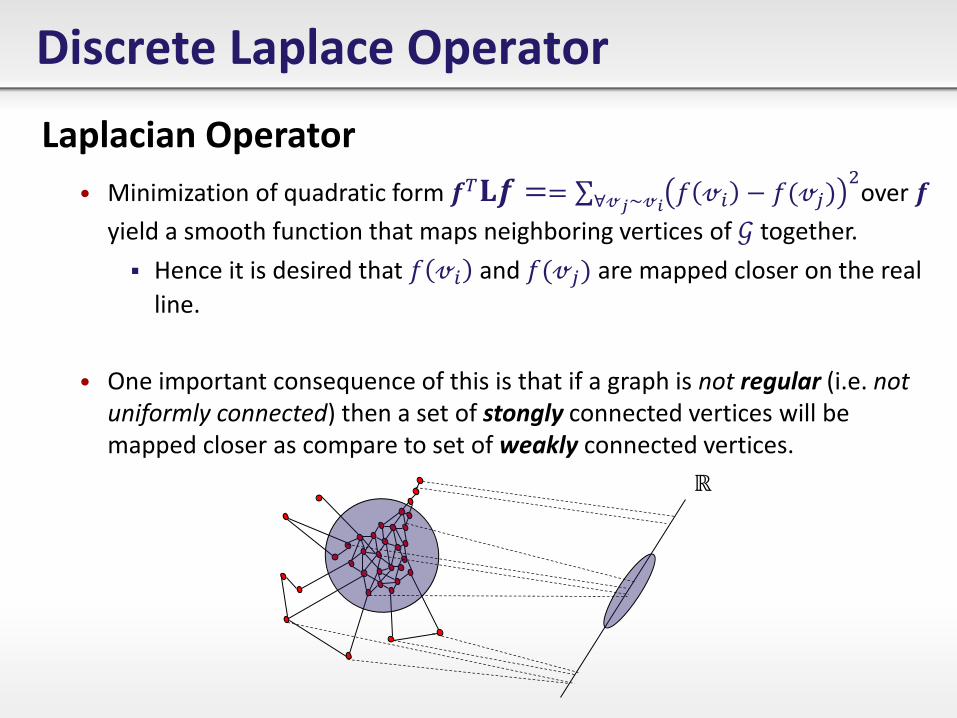
Laplacian Operator
• Minimization of quadratic form 𝒇𝑇𝐋𝒇 == 𝑓 𝓋𝑖 − 𝑓 𝓋𝑗 2
∀𝓋𝑗~𝓋𝑖over 𝒇
yield a smooth function that maps neighboring vertices of 𝒢 together.
Hence it is desired that 𝑓 𝓋𝑖 and 𝑓 𝓋𝑗 are mapped closer on the real
line.
• One important consequence of this is that if a graph is not regular (i.e. not uniformly connected) then a set of stongly connected vertices will be mapped closer as compare to set of weakly connected vertices.
ℝ
Laplacian Eigenvectors
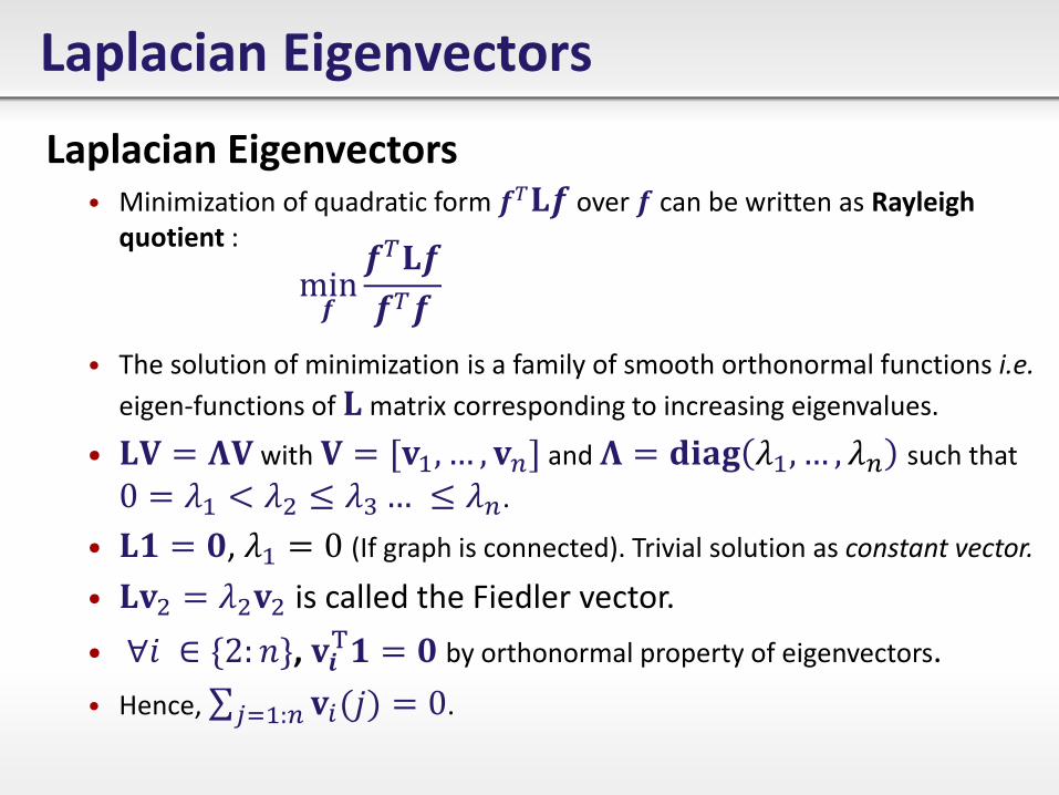
Laplacian Eigenvectors • Minimization of quadratic form 𝒇𝑇𝐋𝒇 over 𝒇 can be written as Rayleigh
quotient :
• The solution of minimization is a family of smooth orthonormal functions i.e.
eigen-functions of 𝐋 matrix corresponding to increasing eigenvalues.
• 𝐋𝐕 = 𝚲𝐕 with 𝐕 = [𝐯1, … , 𝐯𝑛] and 𝚲 = 𝐝𝐢𝐚𝐠 𝜆1, … , 𝜆𝑛 such that
0 = 𝜆1 < 𝜆2 ≤ 𝜆3… ≤ 𝜆𝑛.
• 𝐋𝟏 = 𝟎, 𝜆1 = 0 (If graph is connected). Trivial solution as constant vector.
• 𝐋𝐯2 = 𝜆2𝐯2 is called the Fiedler vector.
• ∀𝑖 ∈ {2: 𝑛}, 𝐯𝒊T𝟏 = 𝟎 by orthonormal property of eigenvectors.
• Hence, 𝐯𝑖 𝑗 𝑗=1:𝑛 = 0.
min𝒇
𝒇𝑇𝐋𝒇
𝒇𝑇𝒇
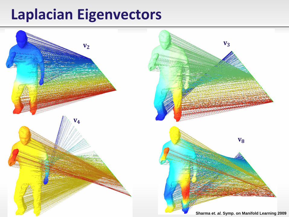
Laplacian Eigenvectors
𝐯𝟐 𝐯𝟑
𝐯𝟒
𝐯𝟖
Sharma et. al. Symp. on Manifold Learning 2009
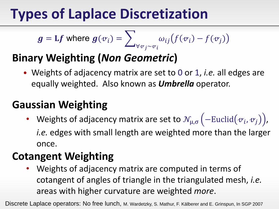
Types of Laplace Discretization
Binary Weighting (Non Geometric) • Weights of adjacency matrix are set to 0 or 1, i.e. all edges are
equally weighted. Also known as Umbrella operator.
Gaussian Weighting • Weights of adjacency matrix are set to 𝒩μ,σ −Euclid 𝓋𝑖 , 𝓋𝑗 ,
i.e. edges with small length are weighted more than the larger once.
Cotangent Weighting • Weights of adjacency matrix are computed in terms of
cotangent of angles of triangle in the triangulated mesh, i.e. areas with higher curvature are weighted more.
𝒈 = 𝐋𝒇 where 𝒈 𝓋𝑖 = 𝜔𝑖𝑗 𝑓 𝓋𝑖 − 𝑓 𝓋𝑗 ∀𝓋𝑗~𝓋𝑖
Discrete Laplace operators: No free lunch, M. Wardetzky, S. Mathur, F. Kälberer and E. Grinspun, In SGP 2007
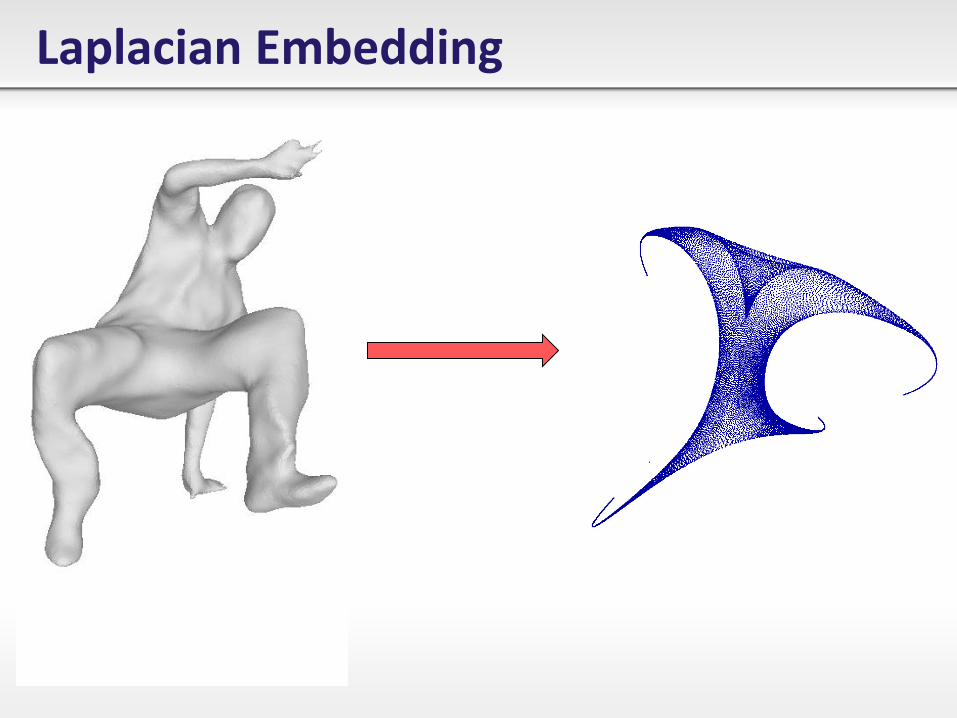
Laplacian Embedding
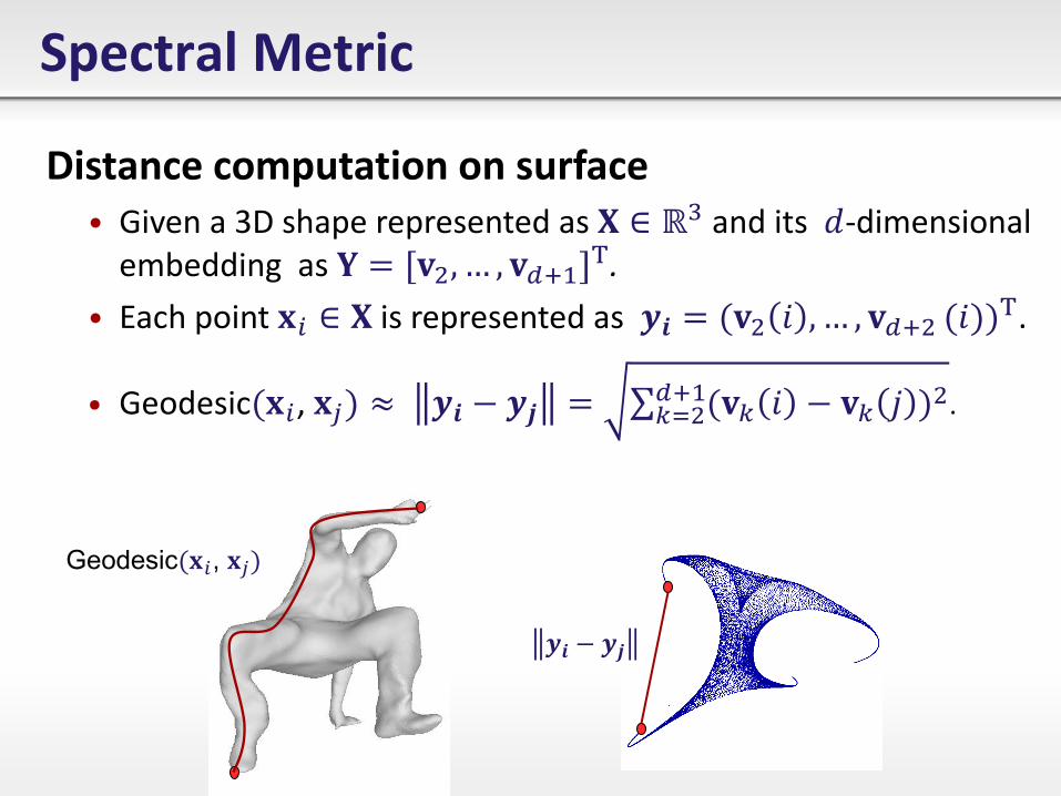
Spectral Metric
Distance computation on surface • Given a 3D shape represented as 𝐗 ∈ ℝ3 and its 𝑑-dimensional
embedding as 𝐘 = [𝐯2, … , 𝐯𝑑+1]T.
• Each point 𝐱𝑖 ∈ 𝐗 is represented as 𝒚𝒊 = 𝐯2 𝑖 , … , 𝐯𝑑+2 𝑖 T.
• Geodesic 𝐱𝑖, 𝐱𝑗 ≈ 𝒚𝒊 − 𝒚𝒋 = 𝐯𝑘 𝑖 − 𝐯𝑘 𝑗 2𝑑+1𝑘=2 .
𝒚𝒊 − 𝒚𝒋
Geodesic 𝐱𝑖, 𝐱𝑗
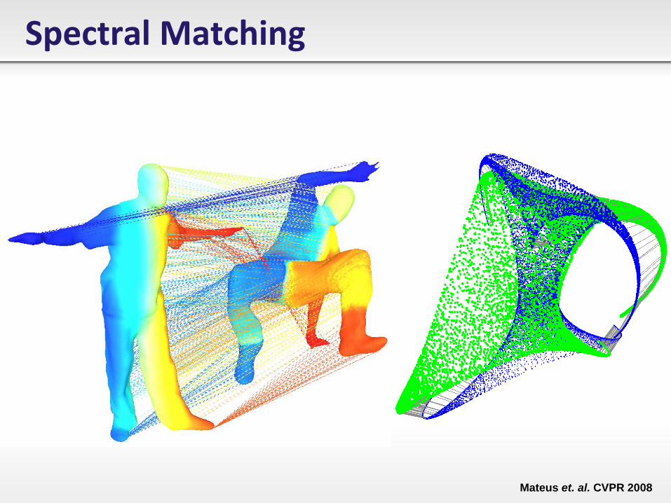
Spectral Matching
Mateus et. al. CVPR 2008

Questions?