GEOMETRICAL QUANTUM MECHANICSRobert Geroch (University of Chicago, 1974)TEXed for posterity by a grad student from an nth-generationphotocopy of the original set of lecture notes. (Aug 1994)

transcribedversion:1/31/2006

Contents

I. Differential Geometry 1

1. Manifolds 1

2. Tensor Algebras 4

3. Tensor fields 7

4. Derivative Operators 10

II. Mechanics 13

5. Configuration Space 13

6. The Cotangent Bundle 18

7. Symplectic Manifolds 20

8. Phase Space 22

9. The Hamiltonian 23

10.Observables; Poisson Bracket 25

11.Canonical Transformations 27

12.Algebraic Observables 31

III. Quantum Mechanics 33

13.Introduction 33

14.Densities. Integrals. 35

15.States 38

16.Observables 40

17.Higher Order Observables 44

18.The Hamiltonian. Dynamics 47

19.Higher Order Observables—Revisited 49

20.Heisenberg Formulation 51

21.The Role of Observables. (Classical Mechanics) 56

22.The Role of Observables. (Quantum Mechanics) 59

23.The Interpretations of Quantum Mechanics 63

24.The Copenhagen Interpretation 65

25.The Everett Interpretation 67

i

GEOMETRICAL QUANTUM MECHANICSRobert Geroch (University of Chicago, 1974)TEXed for posterity by a grad student from an nth-generationphotocopy of the original set of lecture notes. (Aug 1994)

Part I.

Differential Geometry

1. Manifolds

The arena in which all the action takes place in differential geometry is an objectcalled a manifold. In this section, we define a manifold, and give a few examples.

Roughly speaking, a n-dimensional manifold is a space having the “localsmoothness structure” of Euclidean n-space, IRn. (Euclidean n-space is theset consisting of n-tuples, (x1, . . . , xn), of real numbers). The idea, then, is toisolate, from the very rich structure of IRn (e.g., its metric structure, vector-space structure, topological structure, etc.), that one bit of structure we call“smoothness”.

Let M be a set. An n-chart on M consists of a subset U of M and a mappingψ : U → IRn having the following two properties:

1. The mapping ψ is one-to-one.

(That is, distinct points of U are taken, by ψ, to distinct points of IRn.)

2. The image of U by ψ, i.e., the subset O = ψ[U ] of IRn, is open in IRn.

(Recall that a subset O of IRn is said to be open if, for any point x of O,there is a number ǫ > 0 such that the ball with center x and radius ǫ liesentirely within O.)

Let (U,ψ) be a chart. Then, for each point p of U , ψ(p) is an n-tuple of realnumbers. These numbers are called the coordinates of p (with respect to thegiven chart). The range of coordinates (i.e., the possible values of ψ(p) for p

in U) is the open subset O of IRn. By (1), distinct points of U have distinctcoordinates. Thus, ψ represents n real-valued functions on U ; a chart defines alabeling of certain points of M by real numbers.

These charts are the mechanism by which we intend to induce a “localsmoothness structure” on the set M . They are well-suited to the job. Sincea chart defines a correspondence between a certain set of points of M and a cer-tain set of points of IRn, structure on IRn can be carried back to U . To obtain amanifold, we must place on M a sufficient number of charts, and require that,when two charts overlap, the corresponding smoothness structures agree.

Let (U,ψ) and (U ′, ψ′) be two n-charts on the set M . If U and U ′ intersectin M , there is induced on their intersection, V = U ∩ U ′, two “smoothness

1

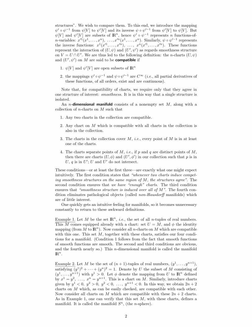
structures”. We wish to compare them. To this end, we introduce the mappingψ′ ψ−1 from ψ[V ] to ψ′[V ] and its inverse ψ ψ′−1 from ψ′[V ] to ψ[V ]. Butψ[V ] and ψ′[V ] are subsets of IRn, hence ψ′ ψ−1 represents n functions-of-n-variables: x′1(x1, . . . , xn), . . . , x′n(x1, . . . , xn). Similarly, ψ ψ′−1 representsthe inverse functions: x1(x′1, . . . , x′n), . . . , xn(x′1, . . . , x′n). These functionsrepresent the interaction of (U,ψ) and (U ′, ψ′) as regards smoothness structureon V = U ∩U ′. We are thus led to the following definition: the n-charts (U,ψ)and (U ′, ψ′) on M are said to be compatible if

1. ψ[V ] and ψ′[V ] are open subsets of IRn

2. the mappings ψ′ ψ−1 and ψ ψ′−1 are C∞ (i.e., all partial derivatives ofthese functions, of all orders, exist and are continuous).

Note that, for compatibility of charts, we require only that they agree inone structure of interest: smoothness. It is in this way that a single structure isisolated.

An n-dimensional manifold consists of a nonempty set M , along with acollection of n-charts on M such that

1. Any two charts in the collection are compatible.

2. Any chart on M which is compatible with all charts in the collection isalso in the collection.

3. The charts in the collection cover M , i.e., every point of M is in at leastone of the charts.

4. The charts separate points of M , i.e., if p and q are distinct points of M ,then there are charts (U, φ) and (U ′, φ′) in our collection such that p is inU , q is in U ′; U and U ′ do not intersect.

These conditions—or at least the first three—are exactly what one might expectintuitively. The first condition states that “whenever two charts induce compet-ing smoothness structures on the same region of M , the structures agree”. Thesecond condition ensures that we have “enough” charts. The third conditionensures that “smoothness structure is induced over all of M”. The fourth con-dition eliminates pathological objects (called non-Hausdorff manifolds) whichare of little interest.

One quickly gets an intuitive feeling for manifolds, so it becomes unnecessaryconstantly to return to these awkward definitions.

Example 1. Let M be the set IRn, i.e., the set of all n-tuples of real numbers.This M comes equipped already with a chart: set U = M , and φ the identitymapping (from M to IRn). Now consider all n-charts on M which are compatiblewith this one. This set M , together with these charts, satisfies our four condi-tions for a manifold. (Condition 1 follows from the fact that smooth functionsof smooth functions are smooth. The second and third conditions are obvious,and the fourth nearly so.) This n-dimensional manifold is called the manifoldIRn.

Example 2. Let M be the set of (n + 1)-tuples of real numbers, (y1, . . . , yn+1),

satisfying (y1)2 + · · · + (yn)2 = 1. Denote by U the subset of M consisting of(y1, . . . , yn+1) with y1 > 0. Let φ denote the mapping from U to IRn definedby x1 = y2, . . . , xn = yn+1. This is a chart on M . Similarly, introduce chartsgiven by y1 < 0, y2 > 0, y2 < 0, . . . , yn+1 < 0. In this way, we obtain 2n + 2charts on M which, as can be easily checked, are compatible with each other.Now consider all charts on M which are compatible with these 2n + 2 charts.As in Example 1, one can verify that this set M , with these charts, defines amanifold. It is called the manifold Sn, (the n-sphere).

2

Example 3. Let M be the set of all orthogonal 3×3 matrices (i.e., matrices whoseinverse is equal to their transpose). Let U consist of the subset M consisting ofmatrices are within 1

10 of the corresponding entries in the unit-matrix. That is,

U consists of orthogonal matrices

a b c

d e f

g h i

with |a−1|, |e−1|, |i−1|, |b|,

|c|, |d|, |f |, |g|, |h| all less than 110 . For such a matrix K, set φ(K) = (b, c, f).

This is a 3-chart on M . Fix any orthogonal matrix P . We define another chart,with U ′ consisting of matrices Q with QP in U , and with ψ′(Q) = ψ(QP ).Thus, for each P we obtain another chart. These charts are all compatible witheach other. The collection of all charts on M compatible with these makes ourset M into a 3-dimensional manifold. This is the manifold of the Lie-groupO(3). (Similarly, other matrix groups are manifolds).

3

2. Tensor Algebras

The natural things to exist on a manifold—the things which will describe thephysics on a manifold—are objects called tensor fields. It is convenient to beginby ignoring manifolds completely. We shall define an abstract tensor algebra—astructure which makes no reference to a manifold. We shall then see, in thefollowing section, that these tensor algebras arise naturally on manifolds.

A tensor algebra consists, first of all, of a certain collection of sets. Weshall label these sets by a script “T” to which there is attached subscripts andsuperscripts from the Latin alphabet. In fact, we introduce a set for everyarrangement of such subscripts and superscripts on T , provided only that thearrangement is such that no index letter appears more than once. Thus, for ex-ample, our collection includes sets denoted by T m

rsba, Tc, T , etc. The collection

does not, however, include a set denoted by Tdcac

r.The elements of these sets will be called tensors. To indicate the particular

set to which a tensor belongs, we shall write each tensor as a base letter withappropriate subscripts and superscripts. Thus, for example, ξr

pasd represents a

tensor, namely, an element of Trpa

sd. Tensors with a single index (e.g., ηc, anelement of Tc) are called vectors; tensors with no indices (e.g., α, an element ofT ) scalars.

The next step in the definition of a tensor algebra is the introduction of fouroperations on these tensors.

1. Addition. With any two tensors which are elements of the same set (i.e.,which have precisely the same index structure), there is associated a thirdtensor, again an element of that same set. This operation will be writtenwith a “+”. Thus, λc

ad + ωcad is an element of T c

ad.

2. Outer Product. With any two tensors having no index letter in common,there is associated a third tensor, an element of the set denoted by “T ”with first the indices of the first tensor, and then the indices of the sec-ond tensor attached. This operation will be indicated by writing the twotensors next to each other. Thus, for example, µwe

rtν

yuc is an element of

Twertyu

c.

3. Contraction. Given any tensor, along with a choice of a particular subscriptand a particular superscript of that tensor, there is associated anothertensor, an element of the set denoted by “T ” with all the indices of theoriginal tensor, except the two chosen ones, attached. This operation isindicated by writing the original tensor with the chosen subscript changedso as to be the same letter as the chosen subscript. Thus, for example,choosing the superscript “c” and the subscript “m” for ξr

dmas

bc, we obtainby contraction the element of Tr

das

b written ξrd

masbm. (Note that the final

tensor is not an element of Trdmas

bm. There is no such set.)

4. Index Substitution. Given any tensor, together with a choice of an indexof that tensor and a choice of a Latin letter which does not appear as anindex of that tensor, there is associated another tensor, an element of theset denoted by “T ” with all the indices of the original tensor, except thatthe chosen index letter is replaced by the chosen letter. This operation isindicated by simply changing the appropriate index letter on the tensor.Thus, for example, if we choose the subscript “c” of ηa

cbn and the Latinletter “r”, the result of index substitution is ηa

rbn, an element of T arbn.

These four are the only (algebraic) operations available on tensors. Whatremains is to write the list of properties these operations satisfy.

1. Conditions on addition. Addition is associative and commutative. Withineach set there is an additive identity (written “0”, with indices sup-pressed), and each tensor has an additive inverse (written with a “−”). In

4

short, each of our sets is an abelian group under addition.

(αab + βa

b) + γab = αa

b + (βab + γa

b)

αab + βa

b = βab + αa

b

αab + 0 = αa

b

αab + (−αa

b) = αab − αa

b = 0

2. Conditions on outer product. Outer product is associative and distributiveover addition.

µab(νcmτr) = (µabνc

m)τr

µab(αnr + βn

r) = µabαnr + µabβn

r

(σnr + τn

r)γab = σnrγab + τn

rγab

3. Conditions on contraction. The operation of contraction commutes withall the operations. Thus, if αa

b + βab = γa

b then αbb + βb

b = γbb. (On

the right is the sum of two elements of T ; on the left, contraction appliedto an element of T a

b.) If µabcrs = σab

cτ rs, then µabars = σab

aτ rs. Ifαa

b = κabdd and βc

d = κbbcd, then αb

b = βdd. (This double contraction

would be written κbbdd.) The result of substituting “r” for “b” in λc

bc isthe same as the result of contracting λa

rc over “a” and “c”.

4. Condition on index substitution. The operation of index substitution com-mutes with all the operations. The result of substituting one index foranother, followed by substituting the other for the one, is the originaltensor.

These conditions are easy to remember because they are suggested by thenotation.

5. The set of scalars, T , is the set of real numbers, and addition and outerproduct for scalars is addition and multiplication of real numbers.

It follows immediately that each of our sets is actually a vector space(over the real numbers). Scalar multiplication is outer product by elementsof T . Furthermore, condition 4 implies that, e.g., T r

ac and T sbn are iso-

morphic vector spaces (the isomorphism obtained by index substitution).Furthermore, conditions 2 and 3 imply that the operation of contractionand outer product are linear mappings on the appropriate vector spaces.

6. Every tensor can be written as a (never unique) sum of outer products ofvectors.

On the outer product µacdr

sαuv, contract “s” with “u”, and “v” with

“r”, to obtain an element of T acd which may be written µa

cdrsαs

r. Thus,every element of T a

cdrs defines a linear mapping from the vector space

Tsr to the vector space T a

cd.

7. T acdr

s consists precisely of the set of linear mappings from Tsr to T a

cd,and similarly for other index combinations. Thus, for example, Ta isthe dual of T a (i.e., the set of linear mappings from T to the reals).Further, T a

b is the set of linear mappings from T b to T a (which, sinceT b is isomorphic to T a, is the same as the set of linear mappings fromT b to T b). From this point of view, αa

bβbc is the composition of a linear-

mapping-from-T c-to-T b with a linear-mapping-from-T b-to-T a to obtaina linear-mapping-from-T c-to-T a. Further, αa

a is the trace operation onlinear mappings.

5

A tensor algebra is a collection of sets, on which four operations are defined,subject to seven conditions, as described above. We remark that the conditionsare redundant. We have proceeded in this way in order to put the basic algebraicfacts about tensors together on an equal footing.

The following central result summarizes much of linear algebra:

Theorem. Given any finite dimensional vector space V , there exists a tensoralgebra with its T a isomorphic to V . Furthermore, an isomorphism betweenthe “T a’s” of two tensor algebras extends uniquely to an isomorphism of thetensor algebras.

In intuitive terms, a tensor algebra produces a framework for describingeverything which can be obtained, starting from a single vector space, usinglinear mappings and tensor products. It equates naturally isomorphic things.It describes neatly the algebraic manipulations available on these objects.

Why didn’t we require that outer product be commutative? Because itisn’t defined. For example, αabβc

d and βcdαab lie in different vector spaces,

so equality is meaningless. We can, however, recover commutativity of outerproduct by introducing an additional convention. Let, for example, τa

bc be atensor, and, by condition 6, write:

τabc = αaβbγc + · · · + µaνbκc.

Then we can associate with this τabc an element, γcα

aβb + · · ·+κcµaνb, of Tc

ab.

Thus, we obtain an isomorphism between T abc and Tc

ab. Similarly, we have an

isomorphism between any “T ” and any other obtained by changing the orderof the indices, preserving their subscript or superscript status. We make use ofthese isomorphisms as follows. We permit ourselves to write equality of elementsof different vector spaces, isomorphic as above, if the elements correspond underthe isomorphism above. By this extended use of equality, for example, µaνb =νbµ

a. Similarly, we allow ourselves to add elements of isomorphic (as above)vector spaces by adding within one of the two spaces. Thus, γa

bc = δba

c + σcba

means “carry σcba to Tb

ac via the isomorphism, and there add to δb

ac”. The

result, carried to T abc via the isomorphism, is equal to γa

bc.As a final example, let ξab be a tensor. Use index substitution to successively

obtain ξac, ξdc, ξda, and ξba. If it should happen that ξab = ξba, then our tensoris called symmetric. If it should happen that ξab = −ξba, then our tensor iscalled antisymmetric. In general, such a tensor will be neither symmetric norantisymmetric. It can always be written uniquely as the sum of a symmetricand an antisymmetric tensor: ξab = 1

2 (ξab + ξba) + 12 (ξab − ξba). These facts are

familiar from matrix algebra.

6

3. Tensor fields

Our next task is to combine our discussion of manifolds with that of tensoranalysis.

Let M be a manifold. A scalar field on M is simply a real-valued function onM . That is, a scalar field assigns a real number to each point of M . It turns out,however, that arbitrary scalar fields aren’t very interesting: what is interestingare things we shall call smooth scalar fields. Let α be a scalar field on M . Todefine smoothness of α, we must make use of the charts on M . Thus, let (U,ψ)be a chart. Then the points of M in U are labeled, by this chart, by coordinates(x1, . . . , xn). Since α is just a function on M (and hence, also a function onU), we may represent α as one real function of the n variables (x1, . . . , xn).Formally, this function is α ψ−1. We say that the scalar field is smooth if,for every chart (in the definition of the manifold M), α ψ−1 (a function of n

variables) is C∞ (all partials of all orders exist and are continuous). We denoteby S the collection of smooth scalar fields on M . It is obvious that sums andproducts of smooth scalar fields yield smooth scalar fields. It is also clear thatthere are many nonconstant smooth scalar fields on M .

We wish next to define the notion of a vector on a manifold. It is convenient,for motivation, to first recall some things about vectors in Euclidean space. Avector in Euclidean space can be represented by its components, (ξ1, . . . , ξn).This representation is not, however, very convenient for a discussion of vectorson a manifold, because of the enormous freedom available on the choice of charts(with respect to which components could be taken) on a manifold. We wouldlike, therefore, to think of some description of vectors in Euclidean space whichrefers less explicitly to components. Let α(x1, . . . , xn) be a smooth functionof n variables, i.e., a smooth function on our Euclidean space. Then we canconsider the directional-derivative of this function in the direction of our vector,evaluated at the origin:

ξ(α) =

(

ξ1 ∂α

∂x1+ · · · + ξn ∂α

∂xn

∣

∣

∣

∣

x=0

(1)

Thus, given a vector in Euclidean space, ξ(α) is a number for each function α.It is immediate from the properties of partial-derivatives that ξ(α), regarded

as a mapping from smooth functions on Euclidean space to the reals, satisfiesthe following conditions:

1. ξ(α + β) = ξ(α) + ξ(β).

2. ξ(αβ) = α|x=0 ξ(β) + β|x=0 ξ(α).

3. If α = const, ξ(α) = 0.

Thus, a vector in Euclidean space defines a mapping (namely, the directionalderivative) from smooth functions on Euclidean space to the reals, satisfyingthe three conditions above. We now establish a sort of converse, to the generaleffect that these three conditions characterize vectors in Euclidean space. Moreprecisely, we claim that:

A mapping from smooth functions on Euclidean space to the reals satisfying thethree conditions above is of the form (1) for some (ξ1, . . . , ξn).

Proof: Suppose we have such a mapping. Define n numbers by ξ1 = ξ(x1),. . . , ξn = ξ(xn). We shall show that, for this choice, (1) is valid for any smoothfunction α. Write such an α in the form

α = α +∑

i

αixi +

∑

ij

αij(x)xixj (2)

7

where α is a constant, the αi (i = 1, . . . , n) are constants, and αij (i, j =1, . . . , n) are smooth. Then, using conditions 1 and 2 above,

ξ(α) = ξ(α)+∑

i

[

ξ(αi)xi + αiξ(x

i)]

+∑

ij

[

ξ(αij)xixj + αijξ(x

j)xi + αijξ(xi)xj

]

.

Now use the condition 3 and evaluate at the origin:

ξ(α) =∑

i

αiξ(xi) =

∑

i

αiξi

This is the left side of Eqn. (1). But, from (2), this is also clearly the right sideof (1). Hence, (1) holds.

We have now completed our component-independent characterization of vec-tors in Euclidean space. This characterization is the motivation for the defini-tion, which follows, of vectors on a manifold.

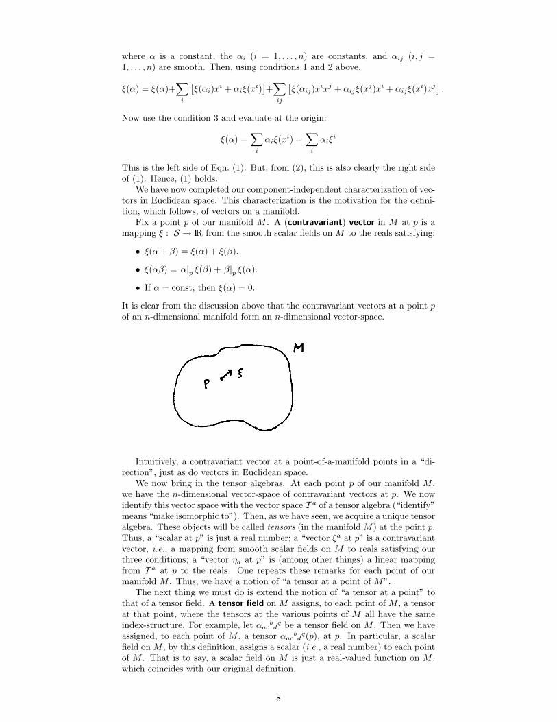
Fix a point p of our manifold M . A (contravariant) vector in M at p is amapping ξ : S → IR from the smooth scalar fields on M to the reals satisfying:

• ξ(α + β) = ξ(α) + ξ(β).

• ξ(αβ) = α|p ξ(β) + β|p ξ(α).

• If α = const, then ξ(α) = 0.

It is clear from the discussion above that the contravariant vectors at a point p

of an n-dimensional manifold form an n-dimensional vector-space.

Intuitively, a contravariant vector at a point-of-a-manifold points in a “di-rection”, just as do vectors in Euclidean space.

We now bring in the tensor algebras. At each point p of our manifold M ,we have the n-dimensional vector-space of contravariant vectors at p. We nowidentify this vector space with the vector space T a of a tensor algebra (“identify”means “make isomorphic to”). Then, as we have seen, we acquire a unique tensoralgebra. These objects will be called tensors (in the manifold M) at the point p.Thus, a “scalar at p” is just a real number; a “vector ξa at p” is a contravariantvector, i.e., a mapping from smooth scalar fields on M to reals satisfying ourthree conditions; a “vector ηa at p” is (among other things) a linear mappingfrom T a at p to the reals. One repeats these remarks for each point of ourmanifold M . Thus, we have a notion of “a tensor at a point of M”.

The next thing we must do is extend the notion of “a tensor at a point” tothat of a tensor field. A tensor field on M assigns, to each point of M , a tensorat that point, where the tensors at the various points of M all have the sameindex-structure. For example, let αac

bdq be a tensor field on M . Then we have

assigned, to each point of M , a tensor αacbdq(p), at p. In particular, a scalar

field on M , by this definition, assigns a scalar (i.e., a real number) to each pointof M . That is to say, a scalar field on M is just a real-valued function on M ,which coincides with our original definition.

8

We observe that the operations defined within a tensor algebra extend from“tensors at a point” to tensor fields. Thus, let αa

b and βab be tensor fields on

M . Their sum, written as αab + βa

b, is a tensor field on M which assigns, tothe point p of M , the sum of the tensors assigned to p by αa

b and βab. That

is, (αab + βa

b)(p) = αab(p) + βa

b(p). Similarly, outer product, contraction, andindex-substitution are well-defined operations on tensor fields. Furthermore, thevarious properties of tensors in a tensor algebra extend to properties of tensorfields. Thus, addition of tensor fields is associative and commutative. The zerotensor field (which assigns to each point the zero-tensor) is an additive identity.Outer products for tensor fields is associative and distributive. Contraction andindex-substitution commute with everything in sight, and so on.

We saw a few pages ago that the notion of a scalar field is not very useful:what is useful is that of a smooth scalar field. This is perhaps not surprising,since the heart of a manifold is its smoothness structure, and one might expectthat compatibility with that smoothness structure should be crucial. Sincescalar fields were rejected in favor of smooth scalar fields, it is natural to askwhether tensor fields can somehow be rejected in favor of smooth tensor fields.This is indeed possible: we now do it.

Consider a contravariant vector field ξa. Let α be any smooth scalar field.Then, for each point p of our manifold, ξa(p) is a contravariant vector at p.Hence, it assigns, to the smooth scalar field α a number. Keeping ξa and α

fixed, and repeating at each point p, we assign a real number to each point ofM . In other words, we obtain a scalar field on M . (This scalar field is, of course,just the directional derivative of α in the direction of the vector field ξa.) Wesay that our contravariant vector field on M can be regarded as a mapping fromsmooth scalar fields on M to scalar fields on M . We say that our contravariantvector field ξa on M is smooth if it assigns, to each smooth scalar field on M

a smooth-scalar field. Thus, we have extended the notion of smoothness fromscalar fields to contravariant vector fields. A vector field ηa will be called smoothif, for each smooth ξa (smoothness for these just defined above), ηaξa is smooth.Finally, a tensor field, e.g., κac

rsq, will be called smooth if κac

rsqξaηcλrω

sρq isa smooth scalar field for any smooth vector fields ξa, ηc, λr, ωs, ρq. Note theway that the notion of smoothness permeates the tensor fields, starting fromthe scalar fields. This sort of thing is common in differential-geometry. Wenow notice that all the tensor operations, applied to smooth tensor fields, yieldsmooth tensor fields.

By the last sentence of the previous paragraph, if one starts with only smoothtensor fields, one never gets anything but smooth fields. It turns out in practicethat it is just the smooth fields which are useful in physics. It is convenient,for this reason, not to have to always carry around the adjective “smooth”. Weshall henceforth omit it. When we say “tensor field”, we mean “smooth tensorfield” unless otherwise specified.

As we shall see shortly, manifolds and tensor fields are remarkably well-suitedfor the description of the arena in which physics takes place, and of the physicsitself, respectively.

9

4. Derivative Operators

What is so great about smoothness? What was gained by our restricting consid-eration to smooth tensor fields? In the case of scalar fields, what we gained byrequiring smoothness was the ability to take (directional) derivatives. This ob-servation (together with the connotation of the word “smooth”) suggests that itshould be possible—and perhaps useful—to introduce the concept of the deriv-ative of a (smooth) tensor field.

We can think of an n-dimensional manifold as similar to an n-dimensionalsurface. Thus, there are n directions in which one can move from a givenpoint. That is, given a tensor field, there are n directions in which one can takethe derivative of that tensor field. These remarks suggest that the operation“taking a derivative” should increase the number of indices of a tensor fieldby one. There is a more explicit way of seeing this. Let α be a scalar field.What should “the derivative of α” look like (as regards index-structure)? Itwould be right, somehow, if the derivative of α had one lowered index, e.g., if itlooked something like ∇aα, for then ξa∇aα, for any contravariant vector fieldξa, would naturally represent the directional derivative of α by ξa. The indexon the “derivative operator” ∇a provides a place to park the index of ξa, i.e., itreflects the freedom in the direction in which the derivative can be taken. Thus,it seems reasonable, as a first try, to try define the “derivative operator” as anoperator, with one down index, which acts on tensor fields. Having made thisobservation, it would be difficult to wind up with any definition for a derivativeoperator other than that which follows.

A derivative operator, ∇a, is a mapping from (smooth) tensor fields to(smooth) tensor fields, which adds one lowered index, and which satisfies thefollowing conditions:

1. The derivatives of the sum of two tensor fields is the sum of the derivatives.For example,

∇a(αrcq + βr

cq) = ∇a(αrcq) + ∇a(βr

cq).

2. The derivative of the outer-product satisfies the Leibniz rule. For example,

∇a(µucdνqv) = µu

cd∇aνqv + νqv∇aµu

cd.

3. The derivative operation commutes with contraction and index substitu-tion. For example, if β = αa

a and γca

b = ∇cαa

b, then ∇cβ = γca

a, andsimilarly for index substitution.

4. For any scalar field α and contravariant vector field ξa the scalar fieldξa∇aα is just the directional derivative.

5. Two derivative operations, applied to a scalar field, commute. That is,∇a∇bα = ∇b∇aα. (Derivatives will not commute, in general, applied totensor fields with more indices.)

Except possibly for the last, these are all natural-looking “derivative-like”conditions. It is easy to define things. What is usually more difficult is to showthat these things exist, and to discover to what extent they are unique. We nowask these questions for derivative operators.

Every manifold one is ever likely to meet possesses a derivative operator.(Precisely, a manifold possesses at least one derivative operator if and only ifit is paracompact.) In fact, it is a nontrivial job just to construct an exampleof a manifold which does not have any derivative operators. We shall hence-forth deal only with manifolds which have at least one derivative operator. (Infact, this restriction will not be needed in any formal sense, but only to makediscussions easier. We shall use the assumed existence of a derivative operator

10

in three cases: to define Lie derivatives, exterior derivatives, and the derivativeoperator defined by a metric. Lie and exterior derivatives exist whether or notderivative operators exist. That the existence of a metric implies the existenceof a derivative operator follows by a comparatively simple argument.)

A more interesting question is this: how unique are derivative operators?It turns out that derivative operators are never unique, but that the non-uniqueness can be expressed in a very simple way. We now proceed to explainthis remark in more detail.

Suppose we had two derivative operators on the manifold M , ∇a and ∇′

a.How are they related? We first consider the difference between their actions on ascalar field: ∇′

aα−∇aα. To draw conclusions about this expression, we contractit with an arbitrary contravariant vector field ξa, to obtain ξa∇′

aα−ξa∇aα. Thisis the difference between two scalar fields. But, by condition 4, in the definitionof a derivative operator, these two scalar fields are the same. So, the difference iszero. That is to say, ξa(∇′

aα−∇aα) vanishes for any ξa. Hence, ∇′

aα−∇aα = 0.That is, ∇′

aα = ∇aα. In words, any two derivative operators have, by condition4, the same action on scalar fields.

We next compare the actions of our two derivative operators on contravariantvector fields. Consider ∇′

aξb − ∇aξb. We cannot conclude, as above, that thisvanishes. However, it is true that this expression is linear in ξb. This followsfrom the following calculation

(∇′

a −∇a)(αξb + ηb)

= ∇′

a(αξb) −∇a(αξb) + ∇′

a(ηb) −∇a(ηb)

= ξb∇′

a(α) + α∇′

a(ξb) − ξb∇a(α) − α∇a(ξb) + (∇′

a −∇a)ηb

= α(∇′

a −∇a)ξb + (∇′

a −∇a)ηb

where, in the last step, we have used the fact that two derivative operatorscoincide on scalar fields. Hence, there is some tensor field Cm

ab such that

∇′

aξb −∇aξb = −Cbacξ

c (3)

for all ξa. In short, derivative operators needn’t be the same on contravariantvector fields, but their difference is expressible simply in terms of a certain tensorfield.

Next, vector fields with one down index (covariant vector fields). Contract∇′

aηb−∇aηb with an arbitrary ξb, and use the properties of derivative operators:

ξb(∇′

aηb −∇aηb) = ∇′

a(ηbξb) − ηb∇

′

aξb −∇aξbηb + ηb∇aξb

= −ηb(∇′

aξb −∇aξb)

= −ηb(−Cbacξ

c)

= +ηmCmabξ

b.

Since ξb is arbitrary, we have

∇′

aξb −∇aξb = ηmCmab (4)

Thus, the actions of our derivative operators on covariant vector fields also differin a simple way, and, furthermore, the same tensor Cm

ab as for contravariantvector fields comes into play.

We next derive, from the fifth property of derivative operators, a certainproperty of this Cm

ab. Let α be any scalar field. Then

∇′

a∇′

bα −∇a∇bα = ∇′

a∇bα −∇a∇bα

= (∇′

a −∇a)∇bα = Cmab∇mα

where, in the first step, we have used the fact that all derivative operatorscoincide on scalars. Now, the left side of this equation remains invariant if “a”

11

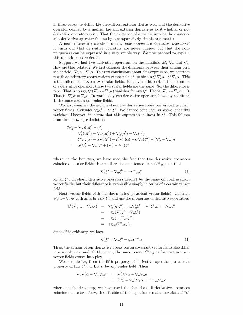
and “b” are switched. So, the right side must. But this holds for all scalar fieldsα, and so

Cmab = Cm

ba (5)

What remains is to extend (3) and (4) to general tensor fields. This isdone as follows. We wish to evaluate, say, (∇′

a − ∇a)αcdrs

u. We contract itwith vectors ξcηdµrνsλ

u. We now differentiate by parts, just as we did in thecalculation preceding Eqn. (4). The result is to shift the derivative operatorsto the vectors. Now use (3) and (4) to get rid of the derivative operators infavor of the Cm

ab. Finally, use the fact that the vectors are arbitrary—so theycan be removed. The result (which, with a little thought, can be seen withoutactually doing the calculation) is

(∇′

a −∇a)αcdrs

u = Cmacαmd

rsu + Cm

adαcmrs

u

−Cramαcd

msu − Cs

amαcdrm

u + Cmauαcd

rsm (6)

Note the form of the right hand of Eqn. (6). There appears a term correspondingto each index of αcd

rsu. Raised indices are treated just like ξb is in (3), while

lowered indices are treated just like ηb is in (4). Thus, Eqns. (3) and (4), whichare now special cases of (6), also make it easy to remember (6). Note also thatthe fact that all derivative operators coincide on scalar fields is a special case ofEqn. (6): no indices leads to no terms on the right.

We conclude that, given two derivative operators, ∇a and ∇′

a, there is a ten-sor field Cm

ab satisfying (5) such that the actions of these derivative operatorsare related by Eqn. (6). A converse is immediate. Suppose we have a derivativeoperator ∇a, and suppose we choose any (smooth) tensor field Cm

ab satisfyingEqn. (5). Then we can define a new operation, ∇′

a, on tensor fields by Eqn. (6).(for (6) can be interpreted now as giving the action of ∇′

a on any tensor field).It is immediate that this ∇′

a, so defined, satisfies the five conditions for a deriv-ative operator. Thus, a derivative operator together with a Cm

ab satisfying (5)defines another derivative operator.

In short, derivative operators are never unique, but we have good controlover the non-uniqueness.

12

GEOMETRICAL QUANTUM MECHANICSRobert Geroch (University of Chicago, 1974)TEXed for posterity by a grad student from an nth-generationphotocopy of the original set of lecture notes. (Aug 1994)

Part II.

Mechanics

5. Configuration Space

The things in the physical world in which we shall be interested will be calledsystems. It is difficult, and probably futile, to try to formulate with any precisionwhat a system is. Roughly speaking, a system is a collection of things (e.g.,objects, particles, fields) under study which, in some sense, do not interact withthe rest of the universe. This splitting of the universe into separate systems onesingles out for individual study is certainly arbitrary to some extent—that isto say, it is probably subject to what is fashionable in physics, and the modeof splitting probably changes as physics evolves. Nonetheless, we have to studysomething, and the things we study we call systems.

Examples of systems:

1. A free, point particle in Euclidean space.

2. A three-dimensional harmonic oscillator. That is, a point particle inEuclidean space, subject to a force directed towards the origin, and havingstrength proportional to the distance of the particle from the origin.

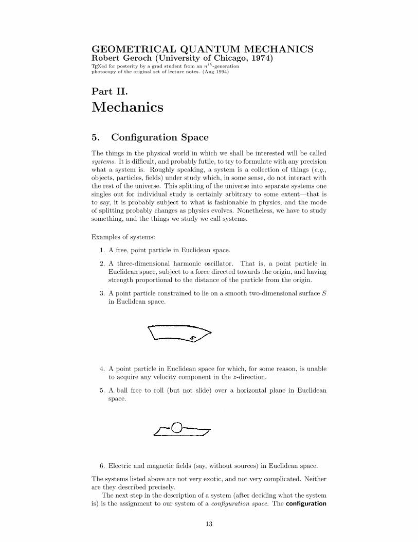
3. A point particle constrained to lie on a smooth two-dimensional surface S

in Euclidean space.

4. A point particle in Euclidean space for which, for some reason, is unableto acquire any velocity component in the z-direction.

5. A ball free to roll (but not slide) over a horizontal plane in Euclideanspace.

6. Electric and magnetic fields (say, without sources) in Euclidean space.

The systems listed above are not very exotic, and not very complicated. Neitherare they described precisely.

The next step in the description of a system (after deciding what the systemis) is the assignment to our system of a configuration space. The configuration

13

space, C, is supposed to be a manifold, the points of which represent “config-urations” of the system. There appears to be no definite rule, given an actualphysical system (e.g., a Swiss watch), for deciding what its space of config-urations, C, should be. Apparently, this is essentially an art. For a simplemechanical system, the configurations are normally distinguished by what canbe seen in an instantaneous photograph. Thus, in examples (1) and (2) above,one would normally choose for the set C the set of “locations of the particle”,i.e., the set of points in Euclidean 3-space. In example (3), one could, I sup-pose, also choose for C the set of points of Euclidean space. But that isn’t aparticularly good choice. One should instead, choose the “locations actuallyavailable to the particle”, i.e., the set of points on the surface S. It is notuncommon, in examples such as (3) above, to first make the “wrong” choicefor configuration space, i.e., to first choose Euclidean space. One then correctsoneself: he realizes that only certain of these configurations, namely, those on S,are actually available to the particle. This process—first choosing “too large”a configuration space, and then imposing restrictions—is called that of intro-ducing holonomic constraints. It is my view that much is gained—and nothinglost—by being careful in the beginning. We shall be careful and, thus, we shallbe able to avoid what are called holonomic constraints.

Configuration space is, as stated above, to be more than just a set of points—it is to be a manifold. That is to say, the set of configurations must be endowedwith a smoothness structure, i.e., with a collection of charts satisfying our fourconditions for a manifold. Here, again, there appears to be no prescription, givena physical system and having decided what its set of configurations is to be, todetermine the manifold structure. There is genuine content in this choice ofsmoothness structure: it, for example, tells us when two configuration are to beregarded as “close”. In examples (1) and (2) above, one would naturally choosefor the manifold structure on C the natural structure on Euclidean space. Thatis, in these examples, one would choose for C the manifold IR3. In example (3),one would select charts appropriate to the embedding of S in Euclidean space.That is, in this example, C would be a 2-dimensional manifold (e.g., a sphere,torus, plane, etc., depending on what S is).

Note that the first two examples are essentially different physical systems,although they have the same configuration space.

Example (4) provides an illustration of these issues. Let us first choosefor the set C the set of points in Euclidean space. What should we choosefor the manifold structure? On the one hand, we could just choose the naturalmanifold structure on Euclidean space. Then C would be IR3. There is, however,another reasonable option. A particle in this example remains in the samez = constant plane all its life. Perhaps, then, we should regard each such planeas a separate “piece” of configuration space. Thus, perhaps we should endowC with the following manifold structure: C is the (disjoint) union of an infinitestack of 2-planes (each labeled by its z value). For this choice, C would betwo-dimensional. For these two choices, we have the same set C, but differentsmoothness structures. There is even a third point of view. One could claimthat the system hasn’t been specified with enough care: that one should alsobe told the z-plane in which the particle beings. This additional information isto be regarded as part of the statement of what the system is. Then, of course,one would choose for C that one plane, i.e., C would be IR2 (since the onlyconfigurations available to the particle need be included in C). Thus, one couldreasonably argue for any of the three configuration spaces for example (4): IR3,the disjoint union of an uncountable collection of IR2’s, or a simple IR2. Mytaste leans mildly toward the second of these three choices.

To specify the “configuration of the system” in example (5), one must statewhere (on the plane) the sphere is, and the orientation of the sphere in space.“Where the plane is” would be represented by a point on the manifold IR2, andthe orientation (which could be described by the rotation necessary to obtain

14

the desired orientation from some fixed orientation) by a point on the manifoldO3 (pp 3). Thus, a natural choice for the configuration space in this examplewould be the product of manifolds IR2 × O3. We shall shortly define preciselythe product of manifolds.)

Example (6) is a bit tricky. We are dealing, here, with vector fields ~E

and ~B in Euclidean space, both of which have vanishing divergence. Here, thedifficulty in giving a prescription for selecting configuration space becomes moreclear. Perhaps the best one can do is try various possibilities for configurationspace, and see which one works best. The one which has been found to workbest is this: choose for C the set of all vector fields ~B in Euclidean space whichhave vanishing divergence. (Holonomic constraint types would say this: choose

first all vector fields ~B, and then restrict to the ones which have vanishingdivergence.) This is the set C; what is the smoothness structure? It turns outthat the only reasonable choice makes C what is called an infinite-dimensionalmanifold. We will not deal here with infinite-dimensional manifolds (becauseof technical complications). Hence, we shall not be able to deal in detail withexample (6).

We summarize: reasonable people could disagree, given a physical system, onwhat configuration space is appropriate. For most systems, however, one choiceis particularly natural, and so we shall allow to speak of the configuration spaceC of a system.

The dimension of the configuration space of a system is called the number

of degrees of freedom of the system.As times marches on, our system evolves, i.e., it passes from one instant of

time to the next, through various configurations. The mathematical descriptionof this situation is via the notion of a curve. A curve on a manifold M is amapping γ : IR → M , where IR is the reals. That is, for each real numbert, γ(t) is a point of M . So, as t sweeps through IR, γ(t) describes our curve.A notion more useful is that of smooth curves, where smoothness for curvesis defined in terms of smooth scalar fields. Let α be a smooth scalar field, soα : M → R. Then α. Then α γ is a mapping from IR to IR, intuitively, “thefunction α evaluated, in terms of t, along the curve”. We say that the curveγ is smooth if, for every smooth scalar field α, α γ (one real function of onevariable) is C∞. Thus, the evolution of our system is described by a smoothcurve γ, with parameter T representing time, on the configuration space C.Thus, whereas examples (1) and (2) have the same configuration space, theactual curves giving the evolution are different in the two examples.

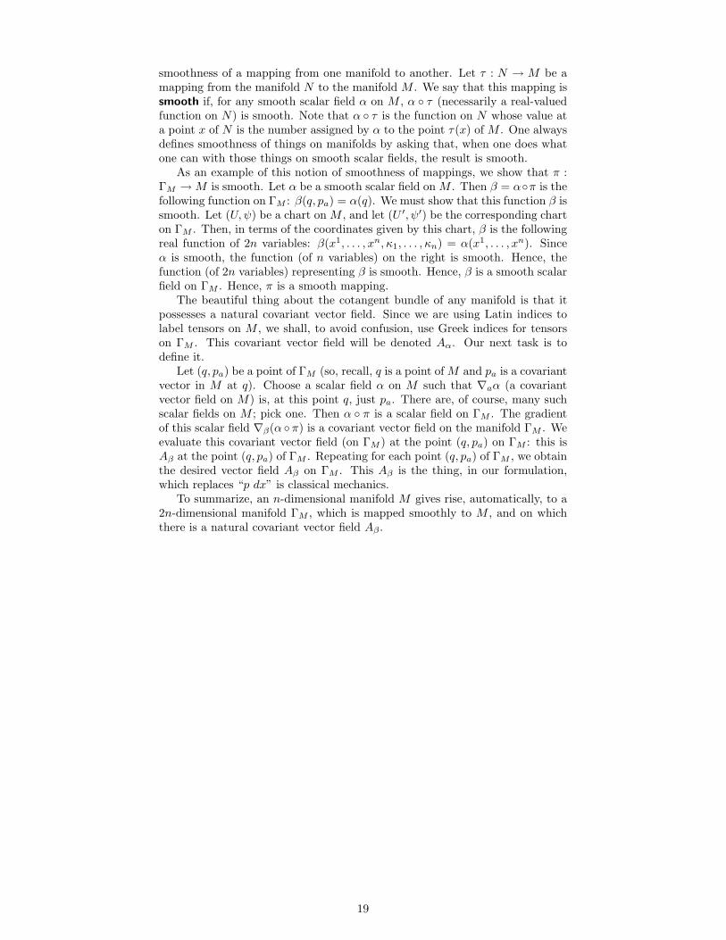
We now need some more mathematics: the notion of the tangent vector toa curve. Let γ be a curve on M . Fix a number t0, and set p = γ(t0). Now letα be a scalar field on M , and consider the number

d

dtα(γ(t))

∣

∣

∣

∣

t0

.

Geometrically, this is the rate of change of the function α, with respect to t,along the curve, evaluated at t0. It is immediate from the properties of thederivative (of functions of one variable) that this mapping from scalar fields onM to the reals satisfies the three conditions on page 8. Hence, this mappingdefines a contravariant vector γa at p. This vector is called the tangent vector

to the curve γ at the point γ(t0). Geometrically, the tangent vector is tangentto the curve, and is large when the curve “covers a lot of M for each incrementof t”.

15

We now return to our system, its configuration space C, and some curve γ

giving the evolution of the system. The tangent vector to this curve at γ(t0) iscalled the velocity of the system at time t0, written va. This just generalizesthe notion of the velocity, e.g., of a particle moving in Euclidean space. Notethat an evolving system, by our description, defines, at each moment of time, aconfiguration and a velocity.

As an illustration of the notion of velocity, we describe the set-up for La-grangian mechanics. Let C be the configuration space for a system. The set ofall pairs (q, va), where q is a point of C and va is a contravariant vector at q

is called the tangent bundle of C. (This is technically not quite correct. Thetangent bundle of a manifold is actually another manifold, having the dimensiontwice that of the original manifold. The set of pairs (q, va) above is actuallyjust the underlying point-set of the tangent bundle.) The starting point forLagrangian mechanics is the introduction of a certain function L(q, va) on thetangent bundle of configuration space. This real-valued function is called theLagrangian of the system. One sometimes writes the Lagrangian as L(x, ∂x).

Are all points of the configuration space accessible to the system? In essen-tially all cases the answer is yes. In fact, that the answer be yes is one goodcriterion to use in selecting configuration space. Are all points of the tangentbundle accessible to the system? (More precisely, is it true that, given anypoint (q, va) of the tangent bundle, there exists a curve in configuration space,describing a possible evolution of the system, such that the curve passes throughq and there has tangent vector va?) For many examples, the answer is yes, butit could be no.

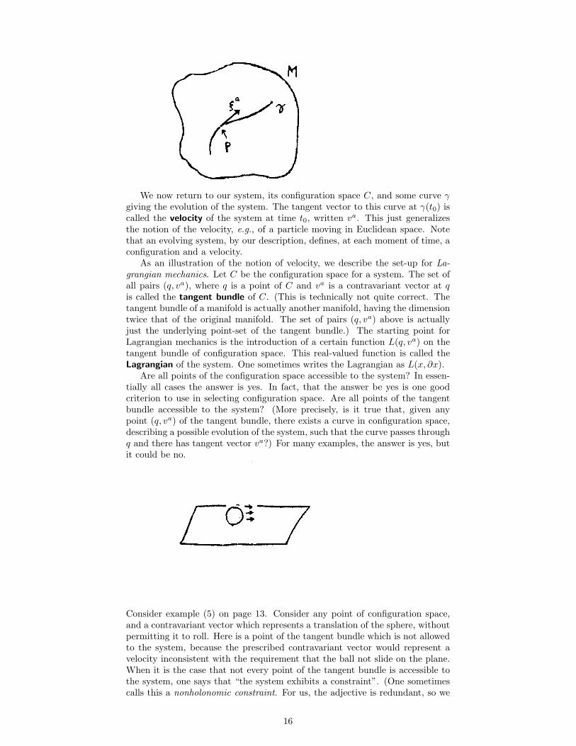
Consider example (5) on page 13. Consider any point of configuration space,and a contravariant vector which represents a translation of the sphere, withoutpermitting it to roll. Here is a point of the tangent bundle which is not allowedto the system, because the prescribed contravariant vector would represent avelocity inconsistent with the requirement that the ball not slide on the plane.When it is the case that not every point of the tangent bundle is accessible tothe system, one says that “the system exhibits a constraint”. (One sometimescalls this a nonholonomic constraint. For us, the adjective is redundant, so we

16

will not use it.) Thus, for example, for our three choices of the configurationspace for example (4), the first has a constraint and the other two do not.There is certainly a sense in which the phrase “has a constraint” represents aproperty of the system itself more than a property of our description of thesystem. It appears to be difficult to make this remark precise. Does the pointof the tangent bundle occupied by the system at one instant of time determineuniquely the future evolution of the system? (More precisely, do two curves,describing a possible evolution of the system, which pass through the samepoint of C for a given time t, and which there have the same tangent vector,necessarily coincide?) Again, examples suggest an answer yes, and this mightbe taken as a criterion for a good choice of configuration space. Again, thisproperty is a rather complicated mixture of an aspect of Nature and an aspectwe impose on Nature by our mode of description.

Suppose we have two systems, S1 and S2, and that we decide to regard themas a single system? (Note that nothing has happened physically: we just lookat things differently.) If C1 and C2 are the configuration spaces of our systems,what should we choose for the configuration space of the combined system? Theanswer is C = C1 × C2, a product of manifolds. We now define this. As a set,C consists of all pairs (p1, p2), where p1 is a point of C1 and p2 is a point ofC2. We introduce charts. Let (U1, ψ1) be a chart on C1, and (U2, ψ2) a charton C2. Consider the chart on C with U = U1 × U2, and, for (p1, p2) in U ,ψ(p1, p2) = (ψ1(p1), ψ2(p2)). (This last expression is an (n1 + n2)-tuple, wheren1 and n2 are the dimensions of C1 and C2, respectively.) The collection ofall charts of C compatible with these makes C a manifold. The dimension ofC is, of course, n1 + n2. Thus, for example, the product of the manifold IR1

and the manifold IR1 is the manifold IR2; The product of IR1 and S1 is thecylinder; The product of S1 and S1 is the torus. Thus, the combination ofsystems is represented, within our description, by the product of configurationspace manifolds.

17

6. The Cotangent Bundle

It is convenient to interrupt briefly our study of mechanics at this point tointroduce a little mathematics.

Let M be an n-dimensional manifold. We define, from M , a new 2n-dimensional manifold ΓM called the cotangent bundle of M . As a point-set,ΓM consists of all pairs (q, pa), where q is a point of M and pa is a covariantvector in M at the point q. (It is not difficult to see, already at this point,why ΓM will turn out to be 2n-dimensional. It takes n dimensions to “locate”q in M , and, having chosen q, n more dimensions to locate pa. (Recall thatthe vector space of covariant vectors at a point of an n-dimensional manifoldis n dimensional.)) What remains is to introduce a collection of charts on thisset ΓM , and to verify that this collection of charts satisfies our four conditionsfor a manifold. Let (U,ψ) be any chart on M , so U is a subset of M and ψ, amapping from U to IRn. We associate, with this chart, a certain chart (U ′, ψ′)(so U ′ will be a subset of ΓM and ψ′ a mapping from U ′ to IR2n) on the set ΓM .For U ′ we choose the collection of all pairs (q, pa) with q in U . Then, for (q, pa)in U ′, we set ψ′(q, pa) = (ψ(q), κ1, . . . , κn) where κ1, . . . , κn are the n numberssuch that

pa = κ1∇ax1 + · · · + κn∇axn

where the right hand side is evaluated at q.We now observe that these charts on ΓM are all compatible with each other,

and that they cover ΓM . The collection of all charts on ΓM compatible withthese makes ΓM a manifold, of dimension 2n.

We repeat this construction in words. A chart on M labels points of M byn-tuples of real numbers. A point of ΓM is a pair (q, pa), where pa is a covariantvector at the point q of M . Half the information needed to specify a point ofΓM , namely q, is already labeled by n numbers, namely, the n numbers ψ(q).For the other half, namely pa, we observe that the gradients of the n coordinatefunctions define, at each point of U (in M), n covariant vectors which spanthe space of covariant vectors at that point. Hence, we can label pa by the n

numbers giving the expression for pa, as a linear combination of the gradientsof the coordinate functions. In this way, we obtain suitable charts on M .

There is a natural mapping, which we write π, from ΓM to M . It is definedby π(q, pa) = q. In words, π is the mapping which “forgets” what the covariantvector pa is, but remembers the point q of M . A picture of this mapping, is thaton the right. Each point q of M is located below a vertical line in ΓM whichrepresents all points of the form (q, pa). Thus, in terms of this picture, π is themapping which sends each point of ΓM straight down to a point of M . It isimmediate, for example, that π is always onto, and that it is one-to-one if andonly if M is zero-dimensional.

This π is our first example of a mapping from one manifold to another.It turns out that some such mappings are more interesting than others. Theinteresting ones are the ones we shall call smooth. Our next task is to define

18

smoothness of a mapping from one manifold to another. Let τ : N → M be amapping from the manifold N to the manifold M . We say that this mapping issmooth if, for any smooth scalar field α on M , α τ (necessarily a real-valuedfunction on N) is smooth. Note that α τ is the function on N whose value ata point x of N is the number assigned by α to the point τ(x) of M . One alwaysdefines smoothness of things on manifolds by asking that, when one does whatone can with those things on smooth scalar fields, the result is smooth.

As an example of this notion of smoothness of mappings, we show that π :ΓM → M is smooth. Let α be a smooth scalar field on M . Then β = απ is thefollowing function on ΓM : β(q, pa) = α(q). We must show that this function β issmooth. Let (U,ψ) be a chart on M , and let (U ′, ψ′) be the corresponding charton ΓM . Then, in terms of the coordinates given by this chart, β is the followingreal function of 2n variables: β(x1, . . . , xn, κ1, . . . , κn) = α(x1, . . . , xn). Sinceα is smooth, the function (of n variables) on the right is smooth. Hence, thefunction (of 2n variables) representing β is smooth. Hence, β is a smooth scalarfield on ΓM . Hence, π is a smooth mapping.

The beautiful thing about the cotangent bundle of any manifold is that itpossesses a natural covariant vector field. Since we are using Latin indices tolabel tensors on M , we shall, to avoid confusion, use Greek indices for tensorson ΓM . This covariant vector field will be denoted Aα. Our next task is todefine it.

Let (q, pa) be a point of ΓM (so, recall, q is a point of M and pa is a covariantvector in M at q). Choose a scalar field α on M such that ∇aα (a covariantvector field on M) is, at this point q, just pa. There are, of course, many suchscalar fields on M ; pick one. Then α π is a scalar field on ΓM . The gradientof this scalar field ∇β(α π) is a covariant vector field on the manifold ΓM . Weevaluate this covariant vector field (on ΓM ) at the point (q, pa) on ΓM : this isAβ at the point (q, pa) of ΓM . Repeating for each point (q, pa) of ΓM , we obtainthe desired vector field Aβ on ΓM . This Aβ is the thing, in our formulation,which replaces “p dx” is classical mechanics.

To summarize, an n-dimensional manifold M gives rise, automatically, to a2n-dimensional manifold ΓM , which is mapped smoothly to M , and on whichthere is a natural covariant vector field Aβ .

19

7. Symplectic Manifolds

As in the previous section, let M be a manifold, and let ΓM be the cotangentbundle of M . Then, as we have seen, there appears on ΓM a certain vector fieldAβ . The curl of this vector field

Ωαβ = ∇αAβ −∇βAα (7)

is called the symplectic tensor field of ΓM . Which derivative operator should weuse in (7)? Fortunately, this is not a decision we have to face, for the right handside of (7) is independent of the derivative operator used. This is immediatefrom (6):

∇′

αAβ −∇′

βAα = CµαβAµ

where, in the last step we have used (5). The right hand side of (7) (except forthe factor of two) is called the exterior derivative in differential-geometry.

The symplectic field will play a central role in our study of mechanics. Thepurpose of this section is to discuss its properties.

The most direct way of getting a quick feeling for the symplectic field is toexpress it in terms of chart. We first do this. Consider a chart on M , writingthe coordinates (x1, . . . , xn). Then, as we saw in the previous section, we obtaina chart on ΓM , with coordinates (x1, . . . , xn, κ1, . . . , κn). Now fix a point (q, pa)of ΓM , and let the coordinates of this point, with respect to our chart above,be (x1, . . . , xn, κ1, . . . , κn). We first express Aβ , at the point (q, pa), in termsof this chart on ΓM . To do this, we just use the definition of Aβ . Consider ascalar field α on M which, expressed in terms of our chart on M takes the form

κ1(x1 − x1) + . . . + κn(xn − xn). (8)

It is immediate from the definition of the κ’s (pp 18), that ∇aα, evaluatedat q, is just pa. Furthermore, because of what π does, the scalar field α π,expressed in terms of our chart on ΓM , is also given by (8). Hence, Aβ |(q,p) =∇β(α π)|(q,p) = (κ1∇βx1 + . . . + κn∇βxn)|(q,p). Since the point (q, pa) wasarbitrary (except that it had to be in our chart on ΓM ), we have

Aβ = κ1∇βx1 + . . . + κn∇βxn. (9)

It is eqn. (9) which suggests we interpret Aβ as “p dx”.We now wish, similarly, to write the symplectic field in terms of these co-

ordinates. This is easy: substitute (9) into (7). Doing this (and using the factthat derivative operators commute when applied to a scalar field), we obtainimmediately

Ωαβ = (∇ακ1)(∇βx1)− (∇αx1)(∇βκ1)+ . . .+(∇ακn)(∇βxn)− (∇αxn)(∇βκn)(10)

This is the desired formula. In intuitive terms, (10) states that Ωαβ has “q-p”components, and “p-q” components, of opposite sign, and that all “q-q” and“p-p” components of Ωαβ vanish.

Finally, we introduce three fundamental properties of the symplectic field:

1. Ωαβ is antisymmetric, i.e., Ωαβ = −Ωβα. This is immediate from thedefinition (7).

2. Ωαβ is invertible, i.e., there exists a (unique) antisymmetric tensor fieldΩαβ such that ΩαγΩβγ = δα

β , where δαβ , the unit tensor, is defined by

the property δαβξα = ξβ for all ξα. (Invertibility for tensors is the tensor

analog of invertibility for matrices.) This property follows, for example,from the explicit expression (10).

3. The curl of Ωβγ vanishes, i.e.,

∇[αΩβγ] = 0 (11)

20

Here, and hereafter, square brackets, surrounding tensor indices, mean “writethe expression with the enclosed indices in all possible orders, affixing a plussign to those that are an even permutation of the original order, and a minussign to those an odd permutation, and, finally, divide by the number of terms”.Thus, in detail, the left hand side of (11) means 1

6 (∇αΩβγ +∇βΩγα +∇γΩαβ −∇αΩγβ −∇βΩαγ −∇γΩβα). The left hand side of (11) is in fact independent ofthe choice of derivative operator, an assertion proven exactly, as we proved thesame assertion for (7). Finally, that (11) is indeed true can be seen, for example,by substituting (10). (Actually, (11) is a consequence of (7). ∇[α∇βAγ] = 0 forany Aγ . To prove this, note that it is true that when Aγ = µ∇γV , and thatany Aγ can be expressed as a sum of such terms of this form.)

More generally, a symplectic manifold is a manifold (necessarily even dimen-sional) on which there is specified a tensor field Ωαβ having the three propertiesabove.

21

8. Phase Space

We return to mechanics. Let C be the configuration space of a system. Thecotangent bundle of C, ΓC , is called the phase space of the system. It was aconsequence of our manner of introducing configuration space that our system,at any instant of time, occupies a particular point of configuration space. Itwill emerge shortly that our system may also be considered to occupy, at eachinstant, a point of phase space. That is to say, our system will “possess”, at eachinstant, a pair (q, pa), where pa is a vector at point q of C. We shall continueto call q the configuration of the system. The covariant vector pa at q will becalled the momentum of the system.

Why does one proceed in this way? At first glance, one might think thatthe most natural thing to do would be to stay in configuration space. Points ofconfiguration space have “concrete physical significance—they represent actualphysical configurations of the actual physical system”. Thus, the physics wouldsomehow be closer to the surface in the mathematics if one could carry outthe entire description directly in terms of the configuration space. However,a technical difficulty arises. As we pointed out in Sect. 5, knowing only thepresent configuration of a system does not suffice to determine what the systemwill do in the future. Roughly speaking, the configuration is half the necessaryinformation. One might, therefore, think of going to the tangent bundle, ofdescribing a system in terms of its configuration q and velocity va. Velocity isalso, in a sense, “concrete”, for one can look at a system (for a short span oftime) and determine its velocity. Thus, by going to the tangent bundle, we couldwork with objects having direct physical significance, and, at the same time, dealwith the 2n variables (q, va) necessary to determine the future behavior of thesystem.

In short, the tangent bundle seems ideal. Why, then, does one choose thecotangent bundle, the phase space, for the description of our system? Theanswer is not very satisfactory: because one has, on the cotangent bundle, thesymplectic field. This field—this additional structure—seems to be necessary towrite the equations which describe mechanics. We shall see that the symplecticfield appears in almost every equation. There is nothing on the tangent bundleanalogous to the symplectic field. The price one pays for the use of this fieldis a more tenuous connection between the mathematics and the actual physics.Suppose, for example, that we have an actual physical system, and that we haveassigned to it some configuration space C. The system is set into action, andwe are permitted to watch the system. We thus obtain a curve in configurationspace. What is the momentum of this system at some instant of time? Thereis no definite way to tell (and, in fact, as we shall see later, there is someambiguity in this assignment). In a sentence, the momentum of a system isa pure kinematical quantity. On the other hand, the cotangent bundle (phasespace) has the same dimension as the tangent bundle. We replace a concretething, velocity, by a more abstract thing, momentum, in order to acquire thesymplectic field for use in equations. What is unsatisfying is that it is not clearwhy Nature prefers additional structure over a direct physical interpretation.

Points of phase space will be called states of the system. Thus, to give thestate of a system, one must specify its configuration and momentum.

22

9. The Hamiltonian

The configuration space concerns kinematics—what can happen. The phasespace is an introduction to the present section, in which we discuss dynamics—what actually does happen.

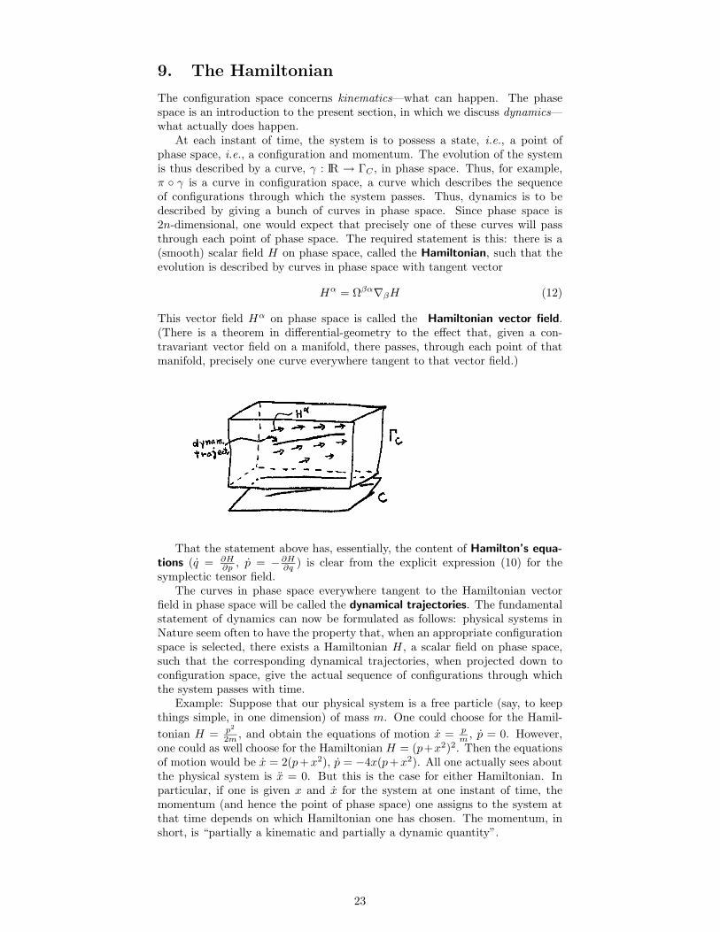
At each instant of time, the system is to possess a state, i.e., a point ofphase space, i.e., a configuration and momentum. The evolution of the systemis thus described by a curve, γ : IR → ΓC , in phase space. Thus, for example,π γ is a curve in configuration space, a curve which describes the sequenceof configurations through which the system passes. Thus, dynamics is to bedescribed by giving a bunch of curves in phase space. Since phase space is2n-dimensional, one would expect that precisely one of these curves will passthrough each point of phase space. The required statement is this: there is a(smooth) scalar field H on phase space, called the Hamiltonian, such that theevolution is described by curves in phase space with tangent vector

Hα = Ωβα∇βH (12)

This vector field Hα on phase space is called the Hamiltonian vector field.(There is a theorem in differential-geometry to the effect that, given a con-travariant vector field on a manifold, there passes, through each point of thatmanifold, precisely one curve everywhere tangent to that vector field.)

That the statement above has, essentially, the content of Hamilton’s equa-

tions (q = ∂H∂p

, p = −∂H∂q

) is clear from the explicit expression (10) for thesymplectic tensor field.

The curves in phase space everywhere tangent to the Hamiltonian vectorfield in phase space will be called the dynamical trajectories. The fundamentalstatement of dynamics can now be formulated as follows: physical systems inNature seem often to have the property that, when an appropriate configurationspace is selected, there exists a Hamiltonian H, a scalar field on phase space,such that the corresponding dynamical trajectories, when projected down toconfiguration space, give the actual sequence of configurations through whichthe system passes with time.

Example: Suppose that our physical system is a free particle (say, to keepthings simple, in one dimension) of mass m. One could choose for the Hamil-

tonian H = p2

2m, and obtain the equations of motion x = p

m, p = 0. However,

one could as well choose for the Hamiltonian H = (p+x2)2. Then the equationsof motion would be x = 2(p+x2), p = −4x(p+x2). All one actually sees aboutthe physical system is x = 0. But this is the case for either Hamiltonian. Inparticular, if one is given x and x for the system at one instant of time, themomentum (and hence the point of phase space) one assigns to the system atthat time depends on which Hamiltonian one has chosen. The momentum, inshort, is “partially a kinematic and partially a dynamic quantity”.

23

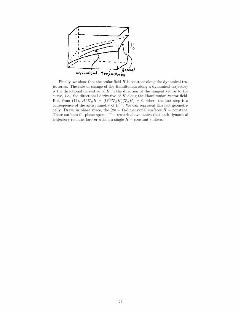
Finally, we show that the scalar field H is constant along the dynamical tra-jectories. The rate of change of the Hamiltonian along a dynamical trajectoryis the directional derivative of H in the direction of the tangent vector to thecurve, i.e., the directional derivative of H along the Hamiltonian vector field.But, from (12), Hα∇αH = (Ωβα∇βH)(∇αH) = 0, where the last step is aconsequence of the antisymmetry of Ωβα. We can represent this fact geometri-cally. Draw, in phase space, the (2n − 1)-dimensional surfaces H = constant.These surfaces fill phase space. The remark above states that each dynamicaltrajectory remains forever within a single H = constant surface.

24

10. Observables; Poisson Bracket

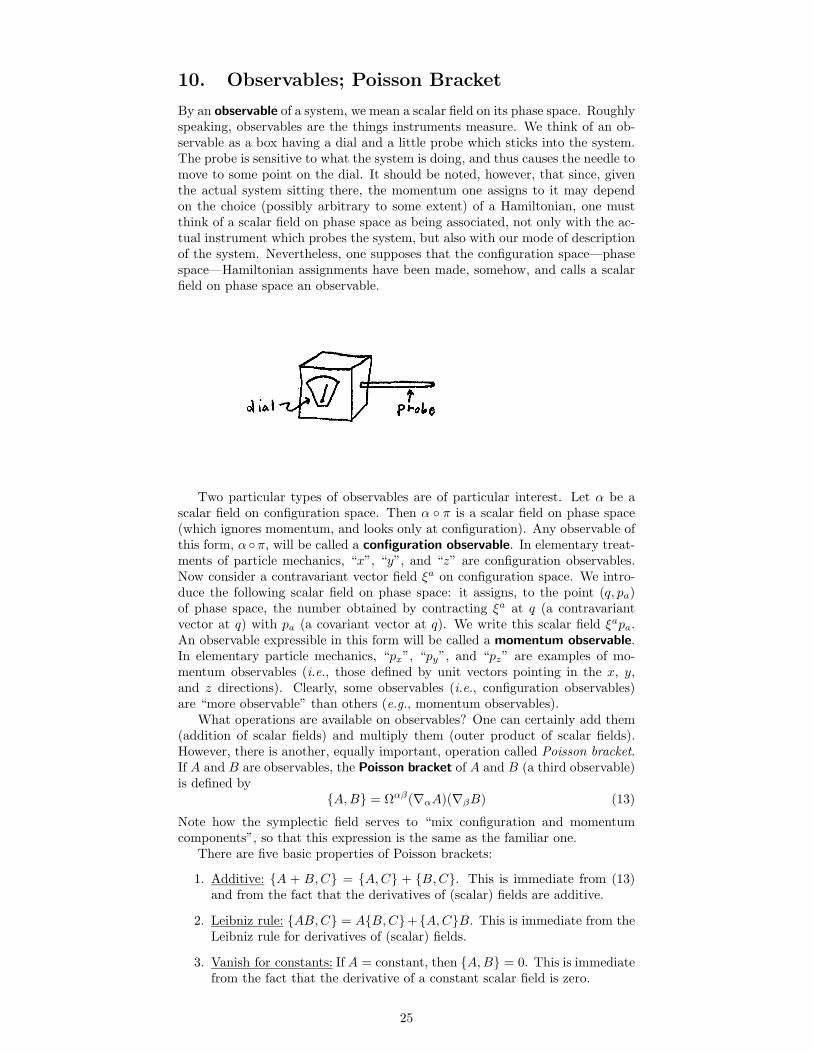
By an observable of a system, we mean a scalar field on its phase space. Roughlyspeaking, observables are the things instruments measure. We think of an ob-servable as a box having a dial and a little probe which sticks into the system.The probe is sensitive to what the system is doing, and thus causes the needle tomove to some point on the dial. It should be noted, however, that since, giventhe actual system sitting there, the momentum one assigns to it may dependon the choice (possibly arbitrary to some extent) of a Hamiltonian, one mustthink of a scalar field on phase space as being associated, not only with the ac-tual instrument which probes the system, but also with our mode of descriptionof the system. Nevertheless, one supposes that the configuration space—phasespace—Hamiltonian assignments have been made, somehow, and calls a scalarfield on phase space an observable.

Two particular types of observables are of particular interest. Let α be ascalar field on configuration space. Then α π is a scalar field on phase space(which ignores momentum, and looks only at configuration). Any observable ofthis form, α π, will be called a configuration observable. In elementary treat-ments of particle mechanics, “x”, “y”, and “z” are configuration observables.Now consider a contravariant vector field ξa on configuration space. We intro-duce the following scalar field on phase space: it assigns, to the point (q, pa)of phase space, the number obtained by contracting ξa at q (a contravariantvector at q) with pa (a covariant vector at q). We write this scalar field ξapa.An observable expressible in this form will be called a momentum observable.In elementary particle mechanics, “px”, “py”, and “pz” are examples of mo-mentum observables (i.e., those defined by unit vectors pointing in the x, y,and z directions). Clearly, some observables (i.e., configuration observables)are “more observable” than others (e.g., momentum observables).

What operations are available on observables? One can certainly add them(addition of scalar fields) and multiply them (outer product of scalar fields).However, there is another, equally important, operation called Poisson bracket.If A and B are observables, the Poisson bracket of A and B (a third observable)is defined by

A,B = Ωαβ(∇αA)(∇βB) (13)

Note how the symplectic field serves to “mix configuration and momentumcomponents”, so that this expression is the same as the familiar one.

There are five basic properties of Poisson brackets:

1. Additive: A + B,C = A,C + B,C. This is immediate from (13)and from the fact that the derivatives of (scalar) fields are additive.

2. Leibniz rule: AB,C = AB,C+A,CB. This is immediate from theLeibniz rule for derivatives of (scalar) fields.

3. Vanish for constants: If A = constant, then A,B = 0. This is immediatefrom the fact that the derivative of a constant scalar field is zero.

25

4. Antisymmetry: A,B = −B,A. This is immediate from (13) and the

fact that Ωαβ is antisymmetric.

5. Jacobi identity: A, B,C+B, C,A+C, A,B = 0. This is notso immediate. We have

A, B,C = Ωαβ(∇αA)(∇β [Ωγδ(∇γB)(∇δC) ] )

= Ωαβ [∇βΩγδ](∇αA)(∇γB)(∇δC)

+ΩαβΩγδ∇αA([∇β∇γB]∇δC + ∇γB[∇β∇δC])(14)

where, in the first step, we have substituted (13), and, in the second,we have expanded using the Leibniz rule for a derivative operator. Nowsuppose we add the right side of (14) to itself three times, switching, eachtime, the order of A, B, and C as described by the Jacobi identity. Thenthe second term on the far right in (14) will cancel with itself. Hence, theJacobi identity will be proven if we can show

Ωβ[α∇βΩγδ] = 0 (15)

because this fact would suffice to kill off the first term on the far right in(14). Since Ωαβ is invertible, (15) is equivalent to

ΩµαΩνγΩσδΩβ[α∇βΩγδ] = 0 (16)

Now differentiate by parts (i.e., use the Leibniz rule for derivative opera-tors):

ΩµαΩνγΩσδΩβα∇βΩγδ

= ΩµαΩνγΩβα∇β(ΩσδΩγδ) − ΩµαΩνγΩβαΩγδ∇βΩσδ

= +∇µΩσν

Finally, using the fact that ∇[αΩβγ] = 0, we obtain (15), and hence theJacobi identity.

The five properties of the Poisson bracket are easy to remember: the firstthree are properties of the derivative of scalar fields, the last two are propertiesof the symplectic field.

Finally, we derive the well-known equation for the rate of change with timeof an observable. Let A be an observable. Then the time rate of change of A

(along a dynamical trajectory) is (by definition of tangent vector) the directionalderivative of A in the direction of the tangent vector to this dynamical trajectory.But this tangent vector is the Hamiltonian vector field. Hence,

A = Hα∇αA = Ωβα(∇βH)(∇αA) = H,A (17)

Note, in particular, that, if we replace “A” by “H” in (17), we obtain, byantisymmetry of the Poisson bracket, H = 0. We have already seen this.

26

11. Canonical Transformations

We begin with a little mathematics. Let M and N be manifolds and let ψ :M → N be a mapping. We say that this ψ is a diffeomorphism if

1. ψ is a smooth mapping,

2. ψ−1, a mapping from N to M , exists (i.e., ψ is one-to-one and onto) andis also a smooth mapping.

Intuitively, a diffeomorphism between M and N makes “M and N identicalmanifolds”. Diffeomorphisms are to manifolds as isomorphisms are to vectorspaces, or homeomorphisms are to topological spaces.

The remark above suggests that a diffeomorphism from M to N should beprepared to carry tensor fields from M to N and back. This in fact is the case.Let α be a scalar field on M . Then α ψ−1 is a scalar field on N . It is sort ofthe “image” on N of α on M ; we write this scalar field ψ(α). We now knowhow to carry scalar fields from M to N . Since tensor fields are built up in termsof scalar fields, it should now be possible to carry tensor fields from M to N .Indeed, consider the following equations:

ψ(ξa∇aα) = ψ(ξa)∇aψ(α) (18)

ψ(ξaηa) = ψ(ξa)ψ(ηa) (19)

ψ(T acrs

dξaηcλrωsκd) = ψ(T a

crs

d)ψ(ξa)ψ(ηc)ψ(λr)ψ(ωs)ψ(κd) (20)

Eqns. (18), (19), and (20) are trying to say that tensor operations commutewith the action of ψ. But we wish to use them as the definition of ψ. Eqn. (18)defines ψ(ξa), i.e., it defines a mapping from contravariant vector fields on M

to contravariant vector fields on N . In words, the definition (18) is this: if ξa

is a contravariant vector field on M , ψ(ξa) is that contravariant vector on N

which, applied (via directional derivative) to a scalar field ψ(α) on N , yields thesame result as that of applying ξa to α (on M), and carrying the result over (viaψ) to N . In short, (18) requires that the operation “directional derivative” beinvariant under the pushing of fields from M to N . Similarly, (19) defines ψ(ηa),i.e., (19) defines a mapping from covariant vector fields on M to covariant vectorfields on N . This definition amounts to requiring that contraction be invariantunder the “pushing action” of ψ. Finally, (20) defines a mapping from arbitrarytensor fields on M to fields on N .

In short, a diffeomorphism from one manifold to another provides a mech-anism for carrying tensor fields from the first manifold to the second. Thismechanism is completely and uniquely determined by the following properties:on scalar fields, it is the obvious thing, and it commutes with all tensor opera-tions.

Now consider a system, with configuration space C, phase space ΓC , sym-plectic structure Ωαβ , and Hamiltonian H. A diffeomorphism ψ : ΓC → ΓC

from phase space to itself which leaves invariant the symplectic field,

ψ(Ωαβ) = Ωαβ (21)

is called a canonical transformation. That is to say, canonical transformationsare mappings from phase space to itself which preserve all of the structure ofinterest there (smoothness, symplectic). Note that canonical transformationsneed not leave the Hamiltonian invariant. When this is the case, i.e., when

ψ(H) = H (22)

the canonical transformation will be called a symmetry. For a moment, re-gard the phase space, and symplectic field as representing “kinematics”, and

27

these things, together with the Hamiltonian, as representing “dynamics”. Thenthe following sentence is both a motivation for, and a summary of, the defini-tions above: canonical transformations are to kinematics as symmetries are todynamics as isomorphisms are to vector spaces.

Because they are difficult to manipulate, one seldom uses canonical trans-formations in practice. Instead, one introduces what are called infinitesimalcanonical transformations. In order to define infinitesimal canonical transfor-mations, we must, again, introduce a few properties of manifolds.

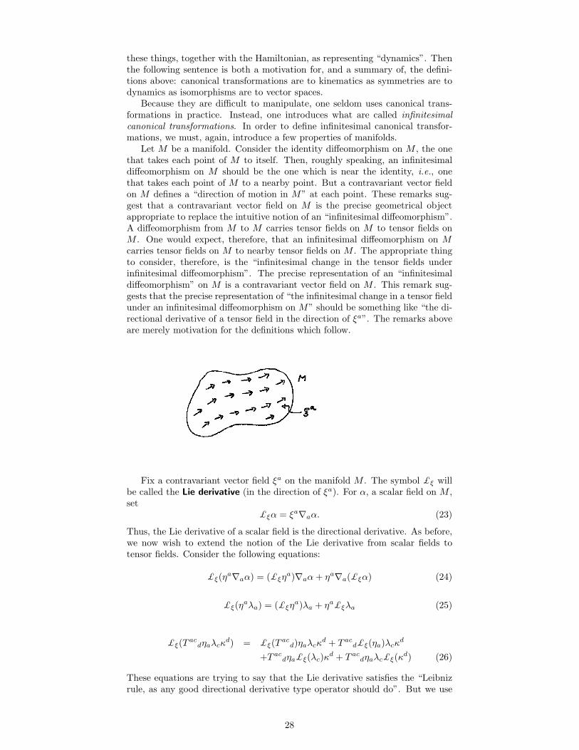
Let M be a manifold. Consider the identity diffeomorphism on M , the onethat takes each point of M to itself. Then, roughly speaking, an infinitesimaldiffeomorphism on M should be the one which is near the identity, i.e., onethat takes each point of M to a nearby point. But a contravariant vector fieldon M defines a “direction of motion in M” at each point. These remarks sug-gest that a contravariant vector field on M is the precise geometrical objectappropriate to replace the intuitive notion of an “infinitesimal diffeomorphism”.A diffeomorphism from M to M carries tensor fields on M to tensor fields onM . One would expect, therefore, that an infinitesimal diffeomorphism on M

carries tensor fields on M to nearby tensor fields on M . The appropriate thingto consider, therefore, is the “infinitesimal change in the tensor fields underinfinitesimal diffeomorphism”. The precise representation of an “infinitesimaldiffeomorphism” on M is a contravariant vector field on M . This remark sug-gests that the precise representation of “the infinitesimal change in a tensor fieldunder an infinitesimal diffeomorphism on M” should be something like “the di-rectional derivative of a tensor field in the direction of ξa”. The remarks aboveare merely motivation for the definitions which follow.

Fix a contravariant vector field ξa on the manifold M . The symbol £ξ willbe called the Lie derivative (in the direction of ξa). For α, a scalar field on M ,set

£ξα = ξa∇aα. (23)

Thus, the Lie derivative of a scalar field is the directional derivative. As before,we now wish to extend the notion of the Lie derivative from scalar fields totensor fields. Consider the following equations:

£ξ(ηa∇aα) = (£ξη

a)∇aα + ηa∇a(£ξα) (24)

£ξ(ηaλa) = (£ξη

a)λa + ηa£ξλa (25)

£ξ(Tac

dηaλcκd) = £ξ(T

acd)ηaλcκ

d + T acd£ξ(ηa)λcκ

d

+T acdηa£ξ(λc)κ

d + T acdηaλc£ξ(κ

d) (26)

These equations are trying to say that the Lie derivative satisfies the “Leibnizrule, as any good directional derivative type operator should do”. But we use

28

them as definitions. Eqn. (24) is the definition of the Lie derivative of a con-travariant vector field (ηa) on M ; Eqn. (25) the definition of the Lie derivative ofa covariant vector field on M ; Eqn. (26) the definition of the Lie derivative of anarbitrary tensor field on M . To summarize, the Lie derivative, “the directionalderivative generalized to tensor fields”, is completely and uniquely character-ized by the following properties: on scalar fields, it is the obvious thing, and itsatisfies Leibniz-type rules.

One actually uses in practice, not the definitions above for the Lie derivative,but more explicit expressions we now derive. We have

ξb∇b(ηa∇aα) = £ξη

a(∇aα) + ηa∇a(ξb∇bα)

(ξb∇bηa)∇aα + ξbηa∇b∇aα = (£ξη

a)∇aα + (ηa∇aξb)∇bα + ηaξb∇a∇bα

(ξb∇bηa)∇aα = (£ξη

a)∇aα + (ηa∇aξb)∇bα

where the first equation results from using (23) in (21), the second equationresults from expanding using the Leibniz rule (for a derivative operator), andthe third equation results from the fact that derivatives commute on scalarfields. Thus, since α is arbitrary in the last equation above, we have

£ξηa = ξb∇bη

a − ηb∇bξa (27)

We now, similarly, use (23) and (27) in (25)

ξb∇b(ηaλa) = (ξb∇bη

a − ηb∇bξa)λa + ηa£ξλa

(ξb∇bηa)∇cα + ξbηa∇b∇aα = (£ξη

a)∇aα + (ηa∇aξb)∇bα + ηaξb∇a∇bα

(ξb∇bηa)∇aα = (£ξη

a)∇aα + (ηa∇aξb)∇bα

Since ηa is arbitrary,£ξλa = ξb∇bλa + λb∇aξb (28)

Finally, using (27) and (28) in (26), we obtain, in precisely the same wayabove,

£ξTab

cd = ξm∇mT abcd − Tmb

cd∇mξa − T amcd∇mξb

+T abmd∇cξ

m + T abcm∇dξ

m (29)

We could just as well have defined the Lie derivative operation by (29). (Notethat (23), (27), and (28) are just special cases, and that (24), (25), and (26)follow immediately from (29).) Eqn. (29) is easily the most useful expressionfor the Lie derivative. Finally, we note that the right hand side of (29) is infact independent of the choice of derivative operator. This is obvious from ourdefinition, but can also be checked directly from (6).

We now again return to our system, with its configuration space, phase space,symplectic structure, and Hamiltonian. An infinitesimal canonical transforma-

tion on the system is a contravariant vector field ξa on phase space, ΓC , suchthat

£ξΩαβ = 0 (30)

An infinitesimal symmetry is an infinitesimal canonical transformation ξa which,in addition, satisfies

£ξH = 0 (31)

Everything in this section so far, except for (29) and these two definitions, canbe regarded as motivation.

There is a crucial formula, which simplifies the discussion of infinitesimalcanonical transformations, namely,

3ξγ∇[αΩβγ] − £ξΩαβ − 2∇[α(Ωβ]γξγ) = 0 (32)

29

To prove (32), we simply expand it

ξγ∇αΩβγ + ξγ∇βΩγα + ξγ∇γΩαβ

−ξγ∇γΩαβ − Ωγβ∇αξγ − Ωαγ∇βξγ

−∇α(Ωβγξγ) + ∇β(Ωαγξγ) = 0

The first term of (32) gives the first three terms above, the second term of(32) the next three terms, and the last term of (32) the last two terms. But theexpansion above holds (the third term cancels the fourth, the first, fifth, andseventh cancel, and the second, sixth, and eighth cancel). Hence (32) is true.

Since the curl of the symplectic field vanishes (Eqn. 11), (32) becomes

£ξΩαβ + 2∇[α(Ωβ]γξγ) = 0 (33)

Thus, ξα is an infinitesimal canonical transformation if and only if the curl ofΩβγξγ vanishes. But (at least, locally) the curl of a covariant vector field ona manifold vanishes if and only if it is a gradient. Thus, ξα is an infinitesimalcanonical transformation if and only if Ωβγξγ = ∇βA for some scalar field A onphase space. Contracting this equation with Ωβα, we find: ξα is an infinitesimalcanonical transformation if and only if ξα = Ωβα∇βA for some A. This A

is called the generator (or generating function) of the infinitesimal canonicaltransformation.

Thus, observables generate infinitesimal canonical transformations. It shouldalso be clear why one often says that “the evolution of the system is the unfoldingof a sequence of infinitesimal canonical transformations”. (We would say: “TheHamiltonian vector field is an infinitesimal canonical transformation.”)

Thus, infinitesimal canonical transformations can be described in terms ofscalar fields on phase space rather than vector fields (an enormous simplifica-tion). What condition must an observable A satisfy in order that the infinitesi-mal canonical transformation it generates be an infinitesimal symmetry? This iseasy to answer. We ask that the Lie derivative of H in the direction of Ωβα∇βA

vanish. That is to say, we ask that (Ωβα∇βA)(∇αH) = 0. That is to say, weask that the Poisson bracket, A,H = 0. But, from (17), this is precisely thestatement that A be constant along each dynamical trajectory, i.e., that A bea constant of the motion. To summarize, we have shown that every constantof the motion generates an infinitesimal symmetry, and that, conversely, everysymmetry is generated by a constant of the motion.

30

12. Algebraic Observables

Recall that the first step in the description of the system was the assignment tothat system of a configuration space. This configuration space then led to phasespace with its symplectic structure. Note, however, that essentially all of thenotions of mechanics relate directly to phase space rather than configurationspace. That is to say, the primary purpose in introducing configuration spacehas been to obtain phase space. In fact, one could just as well have treatedmechanics as follows:

A system is described by a certain symplectic manifold, called phase space,on which there is a certain scalar field, called the Hamiltonian. One then hasdynamical trajectories, Poisson brackets, canonical transformations, etc.

The present section is devoted to certain constructions which use, in an essentialway, the presence of configuration space.

In sect. 10, we introduced configuration and momentum observables. Wewish to generalize this notion. Consider a tensor field Ra1···ar , with r indices,on configuration space, and suppose that this tensor field is symmetric. (Thatis, suppose Ra1···ar = R(a1···ar), where round brackets, surrounding a collectionof tensor indices, mean “add the expression to all expressions obtained by chang-ing the order of the surrounded indices, and divide by the number of terms”.)We associate, with this tensor field, an observable. Let (q, pa) be a point ofphase space. Then, Ra1···ar (q)pa1

· · · paris a number. Thus, we have assigned

a number to each point of phase space, i.e., we have defined an observable. Weshall write this observable Ra1···arpa1

· · · paror sometimes as O(R). For r = 0

(i.e., when Ra1···ar has no indices), we obtain a configuration variable; for r = 1,a momentum observable. Note, however, that we also obtain observables whichare quadratic, cubic, etc., in the momenta.

Our goal is to express, in terms of the tensor fields, the results on variousoperations on these observables.

Evidently, one can add these totally symmetric tensor fields (i.e., Ra1···ar

and Sa1···as) when they have the same number of indices (i.e., when r = s).There is also a product. If Ra1···ar and Sa1···as are two such fields, we definetheir product, written R∩S (indices suppressed), by R(a1···arSar+1···ar+s). Notethat the number of indices in the product is r + s. Obviously, the product isalso associative and commutative, and distributive over addition. Finally, wedefine a bracket relation on such tensor fields. Let [R,S] (indices suppressed)be the tensor field

rRma1···ar−1∇mSar···ar+s−1 − sSma1···as−1∇mRas···ar+s−1 (34)

First note, from (6), that this expression is independent of the choice ofderivative operator. Next, note that the bracket is antisymmetric, additive,and satisfies the Leibniz rule: [R,S] = −[S,R], [R + S, T ] = [R, T ] + [S, T ],[R∩S, T ] = R∩ [S, T ]+ [R, T ]∩S. It is also true (and it can be verified directlyfrom (34)) that this bracket relation satisfies the Jacobi identity: [[R,S], T ] +[[S, T ], R] + [[T,R], S] = 0. Finally, note that, when r = 1, (i.e., when R is avector), our bracket is just the Lie derivative [R,S] = £RS.

We now claim: the three operations (sum, product, bracket) introducedabove on symmetric tensor fields on configuration space correspond preciselyto the three operations (sum, product, Poisson bracket) on the correspondingobservables. That is to say,

O(R + S) = O(R) + O(S) (35)

O(R ∩ S) = O(R)O(S) (36)

O([R,S]) = O(R), O(S) (37)

31

We first note that (35) and (36) are obvious. To prove (37), one first checks,from (10), that it is valid when only configuration and momentum observablesare permitted. But any tensor field can be written as a sum of outer productsof vectors. Inserting such sums in (37), using the Leibniz rule (on the left, forthe bracket; on the right, for the Poisson bracket) and the fact that (37) holdsfor vectors, we obtain (37) in general. This proves our assertion.

Thus, all the operations on observables yields algebraic observables (i.e.,those obtained from tensor fields on configuration space) when applied to alge-braic observables. In fact, nearly every observable one normally deals with inmechanics is algebraic. An example follows.

Consider the Hamiltonian H = gabpapb+Aapa+V , where gab, Aa, and V arefields on configuration space (with, of course, gab symmetric). The first term, forexample, could be the Hamiltonian of a free particle in Euclidean space, wheregab is the usual metric of Euclidean space. The first and third terms could bethe Hamiltonian of a particle in a potential (V ). The first and second termscould be the Hamiltonian of a charged particle (where Aa is a vector potentialfor the magnetic field). There appear, in fact, to be very few, if any, systemswhose Hamiltonian cannot be put into this form. Let us ask when a momentumobservable, ξapa, is a constant of motion for this Hamiltonian. The condition isthat the Poisson bracket of the Hamiltonian and the observable vanish. Thus,we require that ξ, g = 0, ξ,A = 0, ξ, V = 0. That is to say, we require

£ξgab = 0, £ξA

b = 0, £ξV = 0.

But this is just the statement that the “infinitesimal diffeomorphism” on con-figuration space generated by ξa leave invariant the various tensor fields (onconfiguration space) which go into the Hamiltonian.

Suppose our system is a free particle, so Aa = 0 and V = 0. Then, ξapa is aconstant of the motion whenever £ξg

ab = 0, where gab is the metric of Euclideanspace. There are six such vector fields on Euclidean space, representing trans-lations and rotations. The constants of motion associated with translations arewhat are usually called momenta. The constants of motion associated with therotations are what are usually called angular momenta. Now suppose we intro-duce a potential V , and ask which of our constants of motion remain constantsof the motion. It is precisely those which also satisfy £ξV = ξa∇aV = 0. Inother words, it is the symmetries of Euclidean space which also leave invariantthe potential. If, for example, V is spherically symmetric, there will be threesuch vector fields, ξa

1 , ξa2 , and ξa

3 (namely, those which represent rotations aboutthe origin of spherical symmetry of V ). Set J = ξa

1 ∩ ξa1 + ξa

2 ∩ ξa2 + ξa

3 ∩ ξa3 ,

a symmetric, second-rank tensor field on configuration space. By the Jacobiidentity, O(J) is also a constant of the motion (a quadratic one). This constantof the motion is called the squared angular momentum (for a spherically sym-metric system). The introduction of an Aa destroys, in general, these constantsof the motion—unless, of course, the Aa happens to also be invariant under thecorresponding infinitesimal diffeomorphism on configuration space.

Finally, note that constants of the motion remain constants of the motionunder addition, product, and Poisson brackets. This is true, in particular, ofalgebraic constants of the motion.

32

GEOMETRICAL QUANTUM MECHANICSRobert Geroch (University of Chicago, 1974)TEXed for posterity by a grad student from an nth-generationphotocopy of the original set of lecture notes. (Aug 1994)

Part III.

Quantum Mechanics

13. Introduction

Mechanics is pretty, tidy, and natural looking. It suffers, however, from oneserious flaw: Nature does not seem to behave that way. Specifically, quantummechanics has been found to represent a more accurate description of Naturethan classical mechanics. Roughly speaking, quantum mechanics is a “smearedout version of classical mechanics, where the amount of smearing is governedby a certain constant, Planck’s constant h.” This last statement is, even as a“roughly speaking”, somewhat unsatisfactory. It suggests that the principles ofquantum mechanics are somehow to be imposed on a classically defined system,that quantum mechanics is some sort of thin veneer over classical mechanics.Thus, one often speaks of “quantizing” a classical system. (The situation isperhaps analogous to that in which one first treats matter as a continuum,and then “atomizes” it.) Systems, apparently, “really are” quantum systems—classical mechanics is merely a simplified approximation for the limit in whichone is insensitive to the “smearing”. Nonetheless, it is common, presumablybecause classical mechanics makes good contact with everyday life, to regardquantum mechanics as some sort of correction to classical mechanics.

Our goal is to quantize the system discussed in part II, i.e., to write downthe quantum description of various systems, and check that this descriptionreduces, in an appropriate limit, to the classical description. It would perhapsbe more logical, as the above remark suggests, to do part III before part II.We have artificially reversed the order to provide motivation: part II can bemotivated from everyday life, and part III can be motivated from part II.

There are at least three essentially equivalent formulations of quantum me-chanics: Schrodinger, Heisenberg, and algebraic. Essentially equivalent formu-lations, however, need not necessarily be of equal value: one may give betterinsight, be more readily adapted to other contexts, or suggest exotic general-izations, than another. The view is not uncommon that the Schrodinger for-mulation of quantum mechanics is less natural than the others. The reason isthat the Schrodinger formulation seems to fit badly with the principle of rela-tivity. Nonetheless, the Schrodinger formulation does tie in nicely with classicalmechanics, and so we shall begin with this point of view.

Let us, for the moment, regard classical mechanics as consisting of states, ob-servables, and dynamics. The states, of course, are the points of phase space, theobservables scalar fields on phase space. We can regard the states and observ-ables as the kinematics. The dynamics consists of the Hamiltonian dynamicaltrajectories, etc.

Each of these three classical notions has an analog in quantum mechanics.The space of states in classical mechanics is to be replaced by a corresponding(although different) space of states in quantum mechanics. In either case, thesystem is to be regarded as possessing, at each instant of time, one of its pos-sible states. Dynamics plays essentially the same role in quantum mechanicsas in classical mechanics: it is the means by which one describes the successivestates through which a system passes with time. It is with the observables,however, that a significant departure between classical and quantum mechan-

33

ics, apparently, takes place. Classically, an observable assigns a number to eachstate—a feature one might expect to be characteristic of what one means by a“measuring instrument”. It might seem reasonable, therefore, to suppose thatobservables also in quantum mechanics will have this same characteristic prop-erty. However, observables emerge initially in quantum mechanics as mappingsfrom states to states. This mathematical feature is presumably a reflection ofthe following physical fact: observations on a classical system can be performedwith negligible effect on the system observed, while this is not the case for aquantum system. In other words, the mere assignment of a number to eachstate is not enough information to define a quantum observable; one must alsogive information regarding the state into which the system will be thrown by thisact of observation. This “extra information” is carried by having observablesmap states to states rather than to real numbers.

34

14. Densities. Integrals.

The things which can be integrated over a manifold, it turns out, are, not scalarfields, but things called scalar densities. Scalar densities, in turn, represent aspecial case of tensor densities. We introduce here the appropriate definitionsand properties.

Let M be an n-dimensional manifold. An alternating tensor, ǫa1···an , at apoint of M is an n-index contravariant tensor at that point which is antisym-metric, i.e., which reverses sign under interchange of any two of its indices, i.e.,which satisfies ǫ[a1···an] = ǫa1···an . If ǫ and ǫ′ are two alternating tensors at thesame point, with the second nonzero, then there exists a number α such thatǫa1···an = αǫ′

a1···an . (Proof: Choose a basis v1a, . . . , vna, for the covariant vectorsat the point, and note that, by antisymmetry, an alternating tensor is completelyand uniquely determined by the value of the number ǫa1···anv1a1

· · · vnan.) Thus,

the alternating tensors at a point of a manifold form a one-dimensional vectorspace. An alternating tensor field is an n-index, contravariant, antisymmetrictensor field on M , i.e., an assignment (smoothly) of an alternating tensor toeach point of M .

Fix a real number s. A tensor density, e.g., T pbc

w, at a point of M is amapping from alternating tensors ǫa1···an at that point to tensors T p

bcw(ǫ) at

that point such thatT p

bcw(αǫ) = (α)sT p

bcw(ǫ) (38)

for any real number α. The number s is called the weight of the tensor density.Since any two alternating tensors are proportional, (38) implies that a knowledgeof T p

bcw(ǫ) for one nonzero alternating tensor ǫa1···an determines T p

bcw(ǫ) for all

ǫ, and hence, determines the tensor density T pbc

w. Thus, a choice of alternatingtensor at a point defines a one-to-one correspondence between tensor densitiesat that point and tensors at that point. Roughly speaking, a tensor densityis a tensor having certain “scaling behavior” with alternating tensors. Note,from (38), that a tensor density of weight zero is independent of the alternatingtensor. That is to say, tensor densities of weight zero are just ordinary tensors.

Example: Let κa1···anbe a tensor at a point of M . For any alternating

tensor ǫa1···an at this point, set φ(ǫ) = κa1···anǫa1···an . Thus, we have defined a

mapping from alternating tensors at a point to scalars at that point (i.e., to realnumbers). It is immediate that this mapping satisfies (38) with s = 1. Hence,φ(ǫ) is a scalar density of weight +1. More generally, since tensor densities ofweight +1 define, via (38), linear mappings from alternating tensors to tensors,every tensor density of weight +1 can be represented, as above, by a tensor.Similarly, λa1···anb1···bn

ǫa1···anǫb1···bn is a scalar density of weight +2. It is nowclear that every tensor density of positive integral weight can be representedas a tensor. Now let ηa1···an be a nonzero alternating tensor at a point of M .Then, for ǫa1···an another alternating tensor at that point, set χ(ǫ) = α, where α

is the number such that ηa1···an = αǫa1···an . Clearly, this χ(ǫ) (a mapping fromalternating tensors to scalars) is a scalar density of weight −1. Thus, a nonzeroalternating tensor defines a scalar density of weight −1. Similarly, every tensordensity of negative integral weight can be represented by a tensor. The purposeof introducing tensor densities is to enable us to deal with non-integral weights.

A tensor density field on M is a (smooth) assignment of a tensor densityto each point of M , where the weight is the same for each point of M . (Here,of course, “smooth” means that a smooth tensor field results from a smoothalternating tensor field.)

Which of our tensor operations are applicable to tensor density fields? LetT a

cd and T ′acd be tensor density fields, and, for any alternating tensor ǫ, set

(T acd + T ′a

cd)(ǫ) = T acd(ǫ) + T ′a

cd(ǫ). Now let T and T ′ have weights s ands′, respectively. Then, clearly, the right hand side of this equation is a tensordensity (i.e., the right hand side satisfies (38)) only when s = s′. Thus, thesum of two tensor density fields is defined precisely when they have the same

35

weight (and, of course, the same index structure). The weight of the sum isthe weight of each addend. Similarly, (e.g., (T a

cdWpq)(ǫ) = T acd(ǫ)Wpq(ǫ)),

the outer product of any two tensor density fields is defined. The weight ofthe product is the sum of the weights of the factors. (Note that, for weightzero, i.e., for ordinary tensor fields, these operations reduce to ordinary sumand outer product.) Finally, index substitution and contraction are defined inthe obvious way for tensor densities, and, when applied, yield a density of thesame weight. In short, except for the provision that addition is defined onlybetween densities having the same weight, all operations on tensors extend tooperations on tensor densities.

Fix a derivative operator ∇a on M , so this ∇a acts on tensor fields. Wewish to extend this action to tensor densities. Let ǫa1···an be an alternatingtensor field on M . Then ∇aǫa1···an = λaǫa1···an for some covariant vector fieldλa. (Proof: the left hand side of this equation is antisymmetric in a1, · · · , an.But two alternating tensors are proportional.) We now define the derivative ofa tensor density, e.g., T b

cd, by

(∇aT bcd)(ǫ) = ∇a(T b

cd(ǫ)) − sλaT bcd(ǫ) (39)

where s is the weight of T bcd. That is to say, ∇aT b

cd is to be the tensordensity field whose action on any alternating tensor field ǫ is given by theright hand side of (39). We must check that the right hand side of (39) in-deed satisfies (38). To this end, let ǫ′a1···an = αǫa1···an . Then ∇a(ǫ′a1···an) =∇a(αǫa1···an) = α∇a(ǫa1···an) + (∇aα)ǫa1···an . Hence, λ′

a = λa + α−1(∇aα). Wethen have, for the right side of (39),

∇a(T bcd(ǫ

′)) − sλ′

aT bcd(ǫ

′) = ∇a(T bcd(αǫ)) − s(λa + α−1(∇aα))T b

cd(αǫ)

= ∇a(αsT bcd(ǫ)) − s(λa + α−1(∇aα))αsT b

cd(ǫ)

= [αs∇a(T bcd(ǫ)) + (sαs−1(∇aα))T b

cd(ǫ)]

−sλaαsT bcd(ǫ) − sαs−1(∇aα)T b

cd(ǫ)

= αs∇a(T bcd(ǫ)) − sλa(αs)T b

cd(ǫ)

= αs[∇a(T bcd(ǫ)) − sλaT b

cd(ǫ)]

Thus, (39) indeed defines a tensor density field of weight s. To summarize, aderivative operator on tensor fields extends, via (39), to an operator on tensordensity fields, where taking the derivative does not change the weight. Note,from (39), that a derivative operator on tensor density fields is additive andsatisfies the Leibniz rule.

My nth-generation copyof this page had unread-able sections. So, thispage is my attempt to re-construct the content. Ihope that I have main-tained the style of the pre-sentation and that I didnot introduce any errors.(Please check!)

Now suppose that we have two derivative operators, ∇a and ∇′

a, on M ,related via (6). We wish to find the expression, analogous to (6), relating theactions of these operators on tensor densities. Let ǫa1···an be an alternatingtensor field on M . Then, from (6), ∇′

a(ǫa1···an) = ∇a(ǫa1···an) − Cmamǫa1···an .

That is to say, λ′

a = λa − Cmam. Then, (39) implies (∇′

aT bcd − ∇aT b

cd)(ǫ) =(∇′

a −∇a)T bcd(ǫ) + sCm

amT bcd(ǫ). Since, using (6), we know how (∇′

a −∇a)acts on a tensor T b

cd(ǫ), we can expand the first term on the right hand side toobtain (∇′

aT bcd−∇aT b

cd)(ǫ) = −CbamTm

cd(ǫ)+CmacT

bmd(ǫ)+Cm

adTbcm(ǫ)+

sCmamT b

cd(ǫ). Thus, the generalization of (6) is

(∇′

aT bcd −∇aT b

cd) = −CbamTm

cd + CmacT

bmd + Cm

adTbcm

+sCmamT b

cd (40)

In short, things about tensor fields carry over with appropriate (and minor)modifications to things about tensor density fields.

36

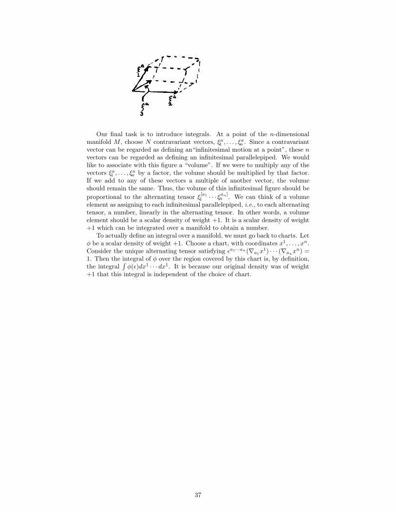
Our final task is to introduce integrals. At a point of the n-dimensionalmanifold M , choose N contravariant vectors, ξa

1 , . . . , ξan . Since a contravariant

vector can be regarded as defining an“infinitesimal motion at a point”, these n

vectors can be regarded as defining an infinitesimal parallelepiped. We wouldlike to associate with this figure a “volume”. If we were to multiply any of thevectors ξa

1 , . . . , ξan by a factor, the volume should be multiplied by that factor.

If we add to any of these vectors a multiple of another vector, the volumeshould remain the same. Thus, the volume of this infinitesimal figure should be

proportional to the alternating tensor ξ[a1

1 · · · ξan]n . We can think of a volume

element as assigning to each infinitesimal parallelepiped, i.e., to each alternatingtensor, a number, linearly in the alternating tensor. In other words, a volumeelement should be a scalar density of weight +1. It is a scalar density of weight+1 which can be integrated over a manifold to obtain a number.

To actually define an integral over a manifold, we must go back to charts. Letφ be a scalar density of weight +1. Choose a chart, with coordinates x1, . . . , xn.Consider the unique alternating tensor satisfying ǫa1···an(∇a1

x1) · · · (∇anxn) =

1. Then the integral of φ over the region covered by this chart is, by definition,the integral

∫

φ(ǫ)dx1 · · · dx1. It is because our original density was of weight+1 that this integral is independent of the choice of chart.

37

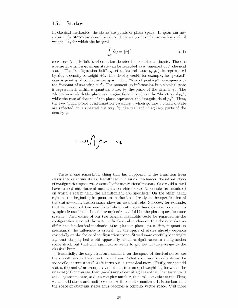
15. States

In classical mechanics, the states are points of phase space. In quantum me-chanics, the states are complex-valued densities ψ on configuration space C, ofweight + 1

2 , for which the integral∫

C

ψψ = ‖ψ‖2 (41)

converges (i.e., is finite), where a bar denotes the complex conjugate. There isa sense in which a quantum state can be regarded as a “smeared out” classicalstate. The “configuration half”, q, of a classical state (q, pa), is representedby ψψ, a density of weight +1. The density could, for example, be “peaked”near a point q of configuration space. The “lack of peaking” corresponds tothe “amount of smearing out”. The momentum information in a classical stateis represented, within a quantum state, by the phase of the density ψ. The“direction in which the phase is changing fastest” replaces the “direction of pa”,while the rate of change of the phase represents the “magnitude of pa”. Thus,the two “point pieces of information”, q and pa, which go into a classical stateare reflected, in a smeared out way, by the real and imaginary parts of thedensity ψ.

There is one remarkable thing that has happened in the transition fromclassical to quantum states. Recall that, in classical mechanics, the introductionof configuration space was essentially for motivational reasons. One could as wellhave carried out classical mechanics on phase space (a symplectic manifold)on which a scalar field, the Hamiltonian, was specified. On the other hand,right at the beginning in quantum mechanics—already in the specification ofthe states—configuration space plays an essential role. Suppose, for example,that we produced two manifolds whose cotangent bundles were identical assymplectic manifolds. Let this symplectic manifold be the phase space for somesystem. Then either of our two original manifolds could be regarded as theconfiguration space of the system. In classical mechanics, this choice makes nodifference, for classical mechanics takes place on phase space. But, in quantummechanics, the difference is crucial, for the space of states already dependsessentially on the choice of configuration space. Stated more carefully, one mightsay that the physical world apparently attaches significance to configurationspace itself, but that this significance seems to get lost in the passage to theclassical limit.

Essentially, the only structure available on the space of classical states arethe smoothness and symplectic structures. What structure is available on thespace of quantum states? As it turns out, a great deal more. Firstly, we can addstates, if ψ and ψ′ are complex-valued densities on C of weight + 1

2 for which theintegral (41) converges, then ψ+ψ′ (sum of densities) is another. Furthermore, ifψ is a quantum state, and κ a complex number, then κψ is another state. Thus,we can add states and multiply them with complex numbers. It is obvious thatthe space of quantum states thus becomes a complex vector space. Still more

38

structure comes from (40). Given two states, ψ and ψ′, we define their inner

product, a complex number, by

〈ψ′ |ψ 〉 =

∫

C

ψ′ψ (42)

It is clear that the inner product satisfies the following properties:

1. 〈ψ |ψ′ + κψ′′ 〉 = 〈ψ |ψ′ 〉 + κ〈ψ |ψ′′ 〉

2. 〈ψ |ψ′ 〉 = 〈ψ′ |ψ 〉

3. 〈ψ |ψ 〉 ≥ 0, equality holding when and only when ψ = 0

More generally, an inner product space is a complex vector space on whichan inner product is defined, satisfying conditions (1), (2) and (3) above. Thus,the space of quantum states is an inner product space. An inner product spacewhich is complete (in an appropriate sense) is called a Hilbert space. The innerproduct spaces which occur in quantum mechanics are almost never complete.However, there exists a procedure for “completing” an inner product space toobtain a Hilbert space. Thus, one sometimes regards the states of a quantumsystem as residing in a Hilbert space (i.e., by suitably completing our space ofstates above). It makes essentially no difference in practice whether one chooseto work in the inner product or the Hilbert space. Primarily to avoid having tointroduce the technical construction of completing, we shall remain in the innerproduct space.

It is natural to ask why the very rich structure of the states of an actualsystem (i.e., the quantum states) become lost in the passage to the classicallimit. This is not at all clear (to me) except for the remark that, for somereason, superposition is lost in the classical limit.

39

16. Observables

We now introduce observables in quantum mechanics. It is convenient to beginsummarizing some mathematics.

Let H be an inner product space. A mapping O : H → H which is linear(i.e., which satisfies O(ψ + κψ′) = O(ψ) + κO(ψ′) for all elements ψ, ψ′ of Hand complex numbers κ) is called an operator on H. Actually, it is convenientto slightly broaden this definition. A subspace D of H will be said to be dense

if, given any element ψ of H and any number ǫ > 0, there is an element ψ′

of D such that ‖ψ − ψ′‖ ≤ ǫ. (Intuitively, a dense subset possesses elementsarbitrarily close to any element of H.) We shall also call linear mappings from adense subspace D of H to H operators. (This is a technical point, necessitatedby the fact that most of the operators we shall need are only defined, in anyreasonable way, on a dense subspace of an inner product space.) An operatorwill be called self-adjoint if, whenever both ψ and ψ′ are in the dense subspaceon which the operator is defined, 〈ψ′ |Oψ 〉 = 〈Oψ′ |ψ 〉.

An observable in quantum mechanics is a self-adjoint operator on the innerproduct space of states.

Of particular interest are observables which have a direct connection withclassical observables. Ideally, one would like to formulate a rule for passingfrom any classical observable (a scalar field on phase space) to a correspondingquantum observable. One has, however, no reason to expect that such a rulewill exist—and, apparently, none does. In fact, it is difficult to think, offhand,of any way whatever to pass from a scalar field on phase space to an operatoron the space of certain densities on configuration space. From a purely math-ematical point of view, it is perhaps surprising that any classical observableshave quantum analogues. Perhaps one should ask for less—ask only that thealgebraic observables go over to quantum mechanics. But, at this stage, eventhis appears to be impossible. It turns out that the classical observables whichdo have simple and unambiguous quantum versions are the configuration andmomentum observables.

Let α be a scalar field on configuration space. Then, as we have seen,α may also be regarded as a scalar field on phase space, i.e., as a classicalobservable. We now define a corresponding quantum observable: Q(α)ψ =αψ. That is to say, Q(α) is the operator on the inner product space of stateswhich, acting on a typical state ψ yields the state obtained by multiplying ψ

(a density on C of weight + 12 ) by α (a density on C of weight 0). The result

is another state, so Q(α) is a mapping from states to states. These operatorsQ(α) will be called configuration observables: they are directly analogous toconfiguration observables in classical mechanics. Note that each Q(α) is self-adjoint: 〈ψ′ |Q(α)ψ 〉 =

∫

ψ′(αψ) =∫ ¯(αψ′)ψ = 〈Q(α)ψ′ |ψ 〉.

The momentum observables are slightly more subtle. Let ξa by a vectorfield on configuration space, so ξapa is a classical momentum observable. Wewish to write down a corresponding quantum observable. The standard rulefor this transition is that of “replacing the classical momentum pa by ( h

i)∇a”.

Thus, one might expect that the appropriate quantum operator is that whoseaction on a state ψ yields ( h

i)ξa∇aψ. However, there are two difficulties with

this choice. Firstly, the operator is not self-adjoint. Indeed,

∫

ψ′(( hi)ξa∇aψ) −

∫

¯(

( hi)ξa∇aψ′

)

ψ = ( hi)

∫

(

ψ′ξa∇aψ + (ξa∇aψ′)ψ)

= ( hi)

∫

(

∇a(ψ′ψξa) − ψ′ψ∇aξa)

= −( hi)

∫

ψ′ψ∇aξa

But the right hand side is not in general zero. Even more serious is the fact that

40

the expression ( hi)ξa∇aψ is not independent of the choice of derivative operator.

In fact, we have from (40)

ξa∇′

aψ − ξa∇aψ =1

2ξaCm

amψ 6= 0.

It is a remarkable fact that a single change in our operator suffices to correctboth of these difficulties. For ξa, a vector field on configuration space, we definean operator, P (ξ), with the following action on a typical state ψ:

P (ξ)ψ = ( hi)(ξa∇aψ + 1

2ψ∇aξa) (43)

It is immediate from the above that the second term on the right in (43) makesthis operator self-adjoint, and, at the same time, produces an operator inde-pendent of the choice of derivative operator. (This last property is vital, for wehave, on configuration space, no preferred derivative operator.) The quantumobservables P (ξ) will be called momentum observables. (Note that the usualangular momentum operators in quantum mechanics are also, by our definition,momentum observables.) The quantum momentum observables are, of course,analogous to the classical momentum observables.

There are three fundamental sets of equations satisfied by these configurationand momentum observables. The first, and easiest, are linearity in the argument:

Q(α + β) = Q(α) + Q(β) (44)

P (ξ + η) = P (ξ) + P (η) (45)

These properties are immediate from the definitions. The second set of equationsare two anti-commutator relations. For A and B operators, we define the anti-

commutator by A,B = AB+BA. We have, immediately from the definition,that Q(α)Q(β) = Q(αβ). Hence,

Q(α), Q(β) = 2Q(αβ) (46)

The anti-commutator between configuration and momentum observables alsotakes a simple form. For ψ a state, we have

P (ξ), Q(α)ψ = P (ξ) (Q(α)ψ) + Q(α) (P (ξ)ψ)

= P (ξ)(αψ) + α( hi)(ξa∇aψ + 1

2ψ∇aξa)

= ( hi)(

(ξa∇a(αψ) + 12 (αψ)∇aξa) + α(ξa∇aψ + 1

2ψ∇aξa))

= ( hi) (ξa(∇aα)ψ + 2αξa∇aψ + αψ∇aξa)

= ( hi) (2αξa∇aψ + ψ∇a(αξa))

= 2( hi)(

αξa∇aψ + 12ψ∇a(αξa)

)

= 2P (αξ)ψ

Hence, since ψ is arbitrary,

P (ξ), Q(α) = 2P (αξ) (47)

Finally, we derive the three (canonical) commutation relations. For A andB operators, we set [A,B] = AB−BA. It is immediate from the definition that

[Q(α), Q(β)] = 0 (48)

Furthermore, we have

[P (ξ), Q(α)]ψ = P (ξ) (Q(α)ψ) − Q(α) (P (ξ)ψ)

= P (ξ)(αψ) − α( hi)(ξa∇aψ + 1

2ψ∇aξa)

= ( hi)(

(ξa∇a(αψ) + 12 (αψ)∇aξa) − α(ξa∇aψ + 1

2ψ∇aξa))

= ( hi) (ξa(∇aα)ψ)

= ( hi)Q(ξa∇aα)ψ

whence[P (ξ), Q(α)] = ( h

i)Q(ξa∇aα) (49)

41

My nth-generation copyof this page had unread-able sections. So, thispage is my attempt to re-construct the content. Ihope that I have main-tained the style of the pre-sentation and that I didnot introduce any errors.(Please check!)

Finally, we obtain the commutation relations for the momentum observables:

[P (ξ), P (η)]ψ

= P (ξ) [P (η)ψ] − P (η) [P (ξ)ψ]

= P (ξ)( hi)[ηb∇bψ + 1

2ψ∇bηb] − P (η)( h

i)[ξb∇bψ + 1

2ψ∇bξb]

= ( hi)[

ξa∇a(( hi)[ηb∇bψ + 1

2ψ∇bηb]) + 1

2 ( hi)[ηb∇bψ + 1

2ψ∇bηb](∇aξa)

]

−( hi)[

ηa∇a(( hi)[ξb∇bψ + 1

2ψ∇bξb]) + 1

2 ( hi)[ξb∇bψ + 1

2ψ∇bξb](∇aηa)

]

= ( hi)2

[

ξa∇a(ηb∇bψ) + 12ξa∇a(ψ∇bη

b) + 12 (ηb∇bψ)∇aξa + 1

2 ( 12ψ∇bη

b)∇aξa

− ηa∇a(ξb∇bψ) − 12ηa∇a(ψ∇bξ

b) − 12 (ξb∇bψ)∇aηa − 1

2 ( 12ψ∇bξ

b)∇aηa]

= ( hi)2

[

(ξa∇aηb − ηa∇aξb)∇bψ + (ξaηb − ηaξb)∇a∇bψ

+[12ψξa∇a(∇bηb) + 1

2ξa(∇aψ)∇bηb] + 1

2 (ηb∇bψ)∇aξa

−[ 12ψηa∇a(∇bξb) + 1

2ηa(∇aψ)∇bξb] − 1

2 (ξb∇bψ)∇aηa]

= ( hi)2

[

(ξa∇aηb − ηa∇aξb)∇bψ + (ξaηb − ηaξb)∇a∇bψ

+ 12ψ[ξa∇a∇bη

b − ηa∇a∇bξb]

]

= ( hi)2

[

(ξa∇aηb − ηa∇aξb)∇bψ + (ξaηb − ηaξb)∇a∇bψ

+ 12ψ[ξa∇a∇bη

b − ηa∇a∇bξb] − 1

2ψ[ξa∇b∇aηb − ηa∇b∇aξb]

+ 12ψ[ξa∇b∇aηb − ηa∇b∇aξb]

]

= ( hi)2

[

(ξa∇aηb − ηa∇aξb)∇bψ + (ξaηb − ηaξb)∇a∇bψ

+ψ[ξa∇[a∇b]ηb − ηa∇[a∇b]ξ

b]

+ 12ψ[∇b(ξ

a∇aηb) − (∇bξa)(∇aηb) −∇b(η

a∇aξb) + (∇bηa)(∇aξb)]

]

= ( hi)2

[

(ξa∇aηb − ηa∇aξb)∇bψ + 12ψ∇b(ξ

a∇aηb − ηa∇aξb)

+(ξaηb − ηaξb)∇a∇bψ + ψ[ξa∇[a∇b]ηb − ηa∇[a∇b]ξ

b]]

= ( hi)2

[

( hi)−1P (£ξη)ψ

+(ξaηb − ηaξb)∇a∇bψ + ψ[ξa∇[a∇b]ηb − ηa∇[a∇b]ξ

b]]

= ( hi)P (£ξη)ψ + ( h

i)2ψ−1∇a∇b(ψ

2ξ[aηb])

where we have used the identity that

ψ−1∇a∇b(ψ2ξ[aηb]) = ψ−1[∇[a∇b](ψ

2ξaηb)]

= ψ−1[ψ2∇[a∇b](ξaηb) + ξaηb∇[a∇b](ψ

2)]

= ψ−1[ψ2(ξa∇[a∇b]ηb + ηb∇[a∇b]ξ

a) + ξaηb(2ψ∇[a∇b]ψ)]

= ψ−1[ψ2(ξa∇[a∇b]ηb − ηa∇[a∇b]ξ

b) + ξaηb(2ψ∇[a∇b]ψ)]

= ψ(ξa∇[a∇b]ηb − ηa∇[a∇b]ξ

b) + 2ξ[aηb]∇a∇bψ

= ψ(ξa∇[a∇b]ηb − ηa∇[a∇b]ξ

b) + (ξaηb − ηaξb)∇a∇bψ

The final result[P (ξ), P (η)] = ( h

i)P (£ξη) (50)

will follow from the calculation above if we show that the last term on thefar right side [i.e., ( h

i)2ψ−1∇a∇b(ψ

2ξ[aηb])] vanishes. Setting F ab = F [ab] =

ψ2ξ[aηb], we have, for an arbitrary scalar field α

∫

α∇a∇bFab = −

∫

(∇aα)∇bFab =

∫

F ab∇a∇bα =

∫

F ab∇[a∇b]α = 0

where we have integrated twice by parts. Hence, ∇a∇bFab = 0, and our result,

(50), follows.

42

Eqns. (48), (49), (50) are called the canonical commutation relations. Notethat, in each case, the commutator of the observables is ( h

i) times the Poisson

bracket of the corresponding classical observables. It is interesting that thequantum observables manage to encompass, in the commutation relations, twofeatures of the classical observables. Firstly, the commutators all contain afactor of h on the right. Thus, in the classical limit (h → 0), the observablescommute, just as do classical observables (where product is outer product). Onthe other hand, the Poisson bracket of classical observables is also reflected inthe commutators.

The fundamental properties of the configuration and momentum observablesare given by Eqns. (44)-(50). These operators and properties are incorporated,in a somewhat peculiar way, into the standard formulation of Schrodinger quan-tum mechanics. Consider, for example, a free particle. One introduces config-uration observables Qx, Qy, and Qz, obtained from the scalar fields x, y, andz on Euclidean space (configuration space). These commute with each other.From (44) and (46), configuration observables associated with any scalar fieldwhich is a polynomial in x, y, z can be constructed as combinations of theobservables Qx, Qy, and Qz. One introduces momentum observables Px, Py,and Pz, defined by unit vector fields in the x, y, and z directions, respectively.Using (45) and (47), the momentum observable associated with any vector fieldin Euclidean space whose Euclidean components are polynomials in x, y, andz can be constructed from Qx, Qy, Qz, Px, Py, Pz. Thus, using (44)-(47), onerecovers essentially (i.e., insofar as polynomials are “essentially all functions”)all of the configuration and momentum observables in terms of just six. Onthese six observables, the canonical commutation relations are imposed. These,of course, are just (48)-(50) in the special cases. Since all other observables areexpressed in terms of these six, the commutation relations on the six suffice toobtain all commutation relations. Our formulae (48)-(50) are just these “gen-eral commutation relations for all configuration and momentum observables”.In short, instead of many observables, subject to (44)-(50), one uses (44)-(47)to reduce to six observables, on which (48)-(50) are imposed. The advantageof our formulation, in my view, is that one avoids making special choices (ofwhich six observables are to be given special status), and treats everything on asimple, one-shot basis. For examples, the angular momentum commutators forthe free particle are special cases of (50).

43

17. Higher Order Observables

The introduction of configuration and momentum observables works out remark-ably well. The definitions are simple and natural, and the resulting operatorssatisfy every condition one could reasonably ask for. One is led by this successto try to carry over into quantum mechanics classical observables which arequadratic, cubic, etc. in momentum. This we attempt, unsuccessfully, in thepresent section.

First note that it is easy to construct observables which involve second, third,etc. derivatives of ψ. For example, let ξa be a vector field on configuration space.Then P (ξ)P (ξ) is an observable whose explicit action, from (43), is

P (ξ)P (ξ)ψ = ( hi)2

[

ξaξb∇a∇bψ + (ξa∇bξb + ξb∇bξ

a)∇aψ

+(12ξa∇a(∇bξ

b) + 14 (∇bξ

b)2)ψ]

More generally, any anti-commutator of observables is an observable. It wouldbe natural to regard P (ξ), P (η) as the quantum observable T abpapb, whereT ab = ξ(aηb). (That is to say, we suitably generalize (46) and (47).) Unfortu-nately, a problem arises. Let λ be any scalar field on configuration space C whichvanishes nowhere (so λ−1 exists). Then it is also true that T ab = (λ−1ξ(a)(ληb)).However, using (46)-(50), it is easily checked in general P (λ−1ξ), P (λη) 6=P (ξ), P (η). More generally, suppose we are given a quadratic classical ob-servable, T abpapb. One can always write T ab as a sum of symmetrized outerproducts of vector fields. One would like to call the corresponding sum of anti-commutators of momentum observables the quantum version of the classicalobservable T abpapb. However, as illustrated above, the resulting quantum ob-servable will in general depend on the decomposition chosen for T ab. In short,we fail, in this way, to associate with classical observables which are quadratic,cubic, etc. in momentum corresponding (unique) quantum observables.

Let T abpapb be a classical observable. We proceed, in a more direct way,to try to associate with this a quantum observable. Clearly, the most generalcandidate is

α(T ab)∇a∇bψ + β(∇aT ab)∇bψ + γ(∇a∇bTab)ψ (51)

where α, β, and γ are real numbers. In order to be acceptable, this candidatemust, at least, satisfy two conditions: it must be self-adjoint, and it must beindependent of the choice of derivative operator.

My nth-generation copyof this page had unread-able sections. So, thispage is my attempt to re-construct the content. Ihope that I have main-tained the style of the pre-sentation and that I didnot introduce any errors.(Please check!)

We ask what α, β, and γ must be in order that each of these conditions, inturn, be satisfied. Evidently, we have

∫

ψ′[α(T ab)∇a∇bψ + β(∇aT ab)∇bψ + γ(∇a∇bTab)ψ]

=

∫

[−α∇a(ψ′T ab)∇bψ + βψ′(∇aT ab)∇bψ + γψ′(∇a∇bTab)ψ]

=

∫

[−α(T ab(∇aψ′)∇bψ + ψ′(∇aT ab)∇bψ)

+βψ′(∇aT ab)∇bψ + γψ′ψ(∇a∇bTab)]

=

∫

[−αT ab(∇aψ′)∇bψ + (β − α)ψ′(∇aT ab)∇bψ + γψ′ψ(∇a∇bTab)]

where, in the first step, we have integrated by parts, and, in the third step, weused the symmetry of T ab. Hence, a necessary and sufficient condition that T

be self-adjoint is that α = β. To investigate behavior under change in the choiceof derivative operator, we use (40):

44

α(T ab)∇′

a∇′

bψ + β(∇′

aT ab)∇′

bψ + γ(∇′

a∇′

bTab)ψ

= αT ab∇′

a(∇bψ + 12Cm

bmψ)

+β(∇aT ab − CaamTmb − Cb

amT am)(∇bψ + 12Cp

bpψ)

+γ(∇′

a(∇bTab − Ca

bmTmb − CbbmT am))ψ

= αT ab(∇a∇bψ + Cmab∇mψ)

+ 12αT ab(Cm

bm(∇aψ + 12Cn

anψ) + (∇′

aCmbm)ψ)

+β(∇aT ab − CaamTmb − Cb

amT am)∇bψ

+ 12β(∇aT ab − Ca

amTmb − CbamT am)Cp

bpψ

+γ(∇a∇bTab − Ca

am∇bTmb)ψ + γ(−∇′

a(CabmTmb + Cb

bmT am))ψ

= αT ab∇a∇bψ + β(∇aT ab)∇bψ + γ(∇a∇bTab)ψ

+αT abCmab∇mψ + 1

2αT abCmbm∇aψ

+(12 )2αT abCm

bmCnanψ + 1

2αT ab(∇′

aCmbm)ψ

−βCaamTmb∇bψ − βCb

amT am∇bψ

+ 12β(∇aT ab − Ca

amTmb − CbamT am)Cp

bpψ

−γ(Caam∇bT

mb + ∇′

a(CabmTmb + Cb

bmT am))ψ

= αT ab∇a∇bψ + β(∇aT ab)∇bψ + γ(∇a∇bTab)ψ

+(∇aψ)((12α − β)T abCm

bm + (α − β)TmbCamb)

+(ψ)(

12αT ab( 1

2CmbmCn

an + ∇′

aCmbm)

+ 12β(∇aT ab − Ca

amTmb − CbamT am)Cp

bp

−γ(Caam∇bT

mb + ∇′

a(CabmTmb + Cb

bmT am)))

My nth-generation copyof this page had unread-able sections. So, thispage is my attempt to re-construct the content. Ihope that I have main-tained the style of the pre-sentation and that I didnot introduce any errors.(Please check!)

It is immediate from this expression that our operator is independent of thechoice of derivative operator precisely when α = β = γ = 0, i.e., when andonly when we have the zero operator. This failure is, of course, just a moresophisticated version of our earlier failure.

Thus, we reach the conclusion that it is only the configuration and momen-tum observables which go over naturally from classical to quantum mechanics.But, as we remarked earlier, what is perhaps surprising is, not that some classi-cal observables have no quantum analogs, but that any at all do. Nevertheless,one is led to ask why the cut-off occurs between linearity and quadratic-ness inmomentum. (Mathematically, it is because different derivative operators onlystart to become really different after the second derivative.) There is, however,a more direct reason.

Recall that every classical observable generates an infinitesimal canonicaltransformation. Let us call a canonical transformation “configuration spacepreserving” if it has the following property: two points of phase space asso-ciated with the same point of configuration space (e.g., (q, pa) and (q, p′a)) aretaken, by the canonical transformation, to points of phase space which again havethis property. Note that a classical observable is a configuration observable ifand only if it assumes the same value on two points of phase space associatedwith the same point of configuration space. Thus, a canonical transformationis configuration space preserving if and only if it takes configuration observ-ables to configuration observables. The infinitesimal version of this statement isthis: the infinitesimal canonical transformation generated by an observable is tobe regarded as configuration space preserving when and only when the Poissonbracket of that observable with any configuration observable is a configurationobservable. But now (37) implies (immediately) that the only observables whichgenerate infinitesimal canonical transformations which are configuration space

45

preserving are the configuration and momentum observables. Thus, these clas-sical observables play a special role.

What is so special about things which are configuration space preserving?Recall that quantum mechanics, as opposed to classical mechanics, requires, notjust phase space, but also configuration space itself. Classical observables which“disrupt” configuration space (i.e., whose infinitesimal canonical transforma-tions are not configuration space preserving) might be expected to be awkwardin quantum mechanics. Indeed, as we have found, they are awkward; they donot seem to carry over from classical to quantum mechanics.

46

18. The Hamiltonian. Dynamics

We now wish to describe the passage of our quantum system, with time, fromone state to another. In classical mechanics, this description is carried out byintroducing a certain observable H, the Hamiltonian. This H then defines thedynamical trajectories, which describe the dynamics. Thus, the most obviousway to proceed is to first to try to replace the classical observable H by somesort of analogous quantum observable.

We are confronted immediately by a serious problem. We have seen inSect. 17 that it is only the configuration and momentum observables whichgo over directly from classical to quantum mechanics. However, the classicalHamiltonian is almost never a configuration or momentum observable. In fact,it is almost always the case that the Hamiltonian contains quadratic terms inthe momenta, i.e., that H takes the form

H = gabpapb + Aapa + V (52)

Such a classical observable, by Sect. 17, does not go over in the obvious way toa quantum observable.

Fortunately, a remarkably simple result intervenes to save the situation. Itis this: On a manifold M , let gab be a symmetric (i.e., gab = g(ab)) tensor fieldwhich is invertible (i.e., for which there exists a field gab such that gamgbm =δa

b). Then, there exists one and only one derivative operator ∇a on M suchthat ∇agbc = 0. Proof: Let ∇′

a be any derivative operator on M . We then have,from (6),

∇agbc = ∇′

agbc + Cbamgmc + Cc

amgbm (53)

We must first show that there is one and only one tensor field Cabc on M such

that the right hand side of (53) vanishes. Indeed, there is one, namely,

Cabc = −gbm∇cg

am − gcm∇bgam + gamgbpgcq∇mgpq (54)

as can be checked by substituting (54) into the right hand side of (53). Supposeboth Ca

bc and Cabc caused the right side of (53) to vanish. Then, setting

Kabc = gam(Cmbc − Cm

bc) we have Kabc = Ka(bc), and, from the vanishing ofthe right side of (53), Kabc = −Kbac. Using alternatively the first and secondof these facts, we have

Kabc = Kacb = −Kcab = −Kcba = Kbca = Kbac = −Kabc

whence Kabc = 0, whence Cabc = Ca

bc. This completes the proof.The idea is to use this result to convert the classical Hamiltonian (52) into

a quantum observable. In order to do this, we must assume that the gab in (52)is invertible. (This condition is certainly satisfied for all the usual systems onetreats in quantum mechanics.) Thus, if the classical Hamiltonian contains a termquadratic in momentum (together, possibly, with terms linear in momentum andindependent of momentum), and if the coefficient of that term, gab, is invertible,we can introduce the corresponding quantum operator

Hψ = ( hi)2gab∇a∇bψ + ( h

i)(Aa∇aψ + 1

2ψ∇aAa) + V ψ (55)

where ∇a in (55) is the unique derivative operator defined by gab (i.e., such that∇cg

ab = 0). We needn’t be concerned with whether or not the right side of (55)is independent of derivative operator (it isn’t), because the classical Hamiltonianprefers one derivative operator. Note that since ∇agbc = 0, the first term on theright in (55) is the same as ( h

i)2∇a(gab∇bψ), and the same as ( h

i)2∇a∇b(g

abψ).(In more conventional language, with this choice of derivative operator, there isno factor ordering problem.) That is to say, if T ab in (51) is replaced by gab, thelast two terms on the right vanish. It is now immediate that from the discussionfollowing (51) that the operator (55) is self-adjoint.

47

Thus, if the classical Hamiltonian is of the form (52), with gab invertible,we can introduce a unique corresponding quantum Hamiltonian (55). As far asI am aware, it is only when the classical Hamiltonian satisfies these conditionsthat one can “quantize” a classical system. Perhaps one should take the point ofview that systems (i.e., quantum theory) operate only within this regime. Whatis then somewhat mysterious is why it should be that, when one passes to theclassical limit, the description has a very natural generalization (i.e., to Hamil-tonians other than (52)) which is completely lost within quantum mechanicsitself. Alternatively, one could take the following view. In quantum mechanics,there is a Hamiltonian observable, which is of finite differential order. A systemdescribed by such a Hamiltonian can, in the classical limit, be described by aclassical Hamiltonian algebraic in the momenta. It just happens that it is onlywhen the original quantum Hamiltonian was of second differential order thatone can pass uniquely back from classical to the quantum description. But, apriori, one might not have expected to be able to pass from the classical descrip-tion, uniquely, to the quantum description in any case. It just happens that,in the quadratic case, no essential information gets lost in the classical limit.(Nature, however, tries to confuse use by making most quantum Hamiltoniansof second differentiable order, so we get used to the idea that we should be ableto recover the quantum description from its classical limit.)

A useful simplification becomes available in the presence of the Hamil-tonian (55). We claim: there are just two alternating tensors (differing onlyin sign) satisfying:

ga1b1 · · · ganbnǫa1...anǫb1...bn = n!

That the left side of this equation is nonzero for any nonzero alternating tensorfollows from the fact that gab is invertible. (This is the tensor statement of thefact from matrix algebra that an invertible matrix has nonzero determinant.)But any multiple of an alternating tensor is an alternating tensor: hence, thereexists an alternating tensor satisfying the above. That there are just two, differ-ing in sign, follows from the fact that, if ǫ and αǫ satisfy the above, then α2 = 1,whence α = ±1. Thus, our claim is proved. We can use this preferred alter-nating tensor (pick one) to reduce density fields to tensor fields. Thus, insteadof a density ψ (a mapping from alternating tensors to scalars), we can evaluatethis ψ on our preferred alternating tensor ǫa1...an , to obtain a complex scalarfield ψ(ǫ). Similarly, all tensor densities can be “evaluated on ǫ” to yield tensorfields. Note, furthermore, that, taking the derivative of the equation above,using the derivative operator defined by gab, we obtain ∇aǫa1...an = 0. Hence,λa = 0 in (39). That is to say, if we use the derivative operator defined bygab, and evaluate tensor densities on the preferred alternating tensor to obtaintensor fields, we can replace derivatives of such densities by derivatives of thecorresponding tensor fields. (In other words, the operations “evaluate on thepreferred alternating tensor” and “take the derivative by the preferred derivativeoperator” commute.)

Our final task is to write down the equation describing the dynamics of oursystem. At each time t, the system is to be in some state, ψ(t), where ψ(t) is(by the previous paragraph) a complex scalar field on configuration space C, foreach t. The dynamical equation, called Schrodinger’s equation, is

− ( hi)

d

dtψ = Hψ (56)

This gives the time rate of change of ψ in terms of ψ at one instant of time.Hence, (56) determines ψ(t) for all t, given ψ(t0) at one fixed time, t0.

48

19. Higher Order Observables—Revisited

We have seen in Sect. 17 that classical observables which are of order quadraticor higher in momentum do not lead to quantum observables. The difficultywas this: no expression could be found for the quantum observable which wasindependent of the choice of derivative operator. But, in Sect. 18, we observedthat the presence of a (classical) Hamiltonian quadratic in momentum leads,among other things, to a natural, unique derivative operator. Thus releasedfrom what was the primary difficulty in Sect. 17, we return to the question ofthat section.

We begin with the quadratic case. Let T abpapb be a classical observable.Then, using the unique derivative operator defined by the Hamiltonian, wehave the following corresponding quantum observable

12 ( h

i)2[T ab∇a∇b + (∇a∇bT

ab) + γ(∇bTab)∇a] (57)

where γ is any real number. This operator is self-adjoint for all γ, but, of course,is independent of the choice of ∇a for no γ. In short, one has, in the presenceof a preferred derivative operator, a one-parameter family of candidates for thequantum version of the observable T abpapb. It is clear that this situation contin-ues into higher-order observables. A classical observable of quadratic or higherorder in momentum leads, in the presence of a preferred derivative operator, toa family of “corresponding” quantum observables depending on some arbitraryconstant parameters.

Thus, one before had no quantum versions of higher-order classical observ-ables —one now has many. It is natural, in such a situation, to attempt toimpose some additional conditions on our quantum observables in order to ob-tain uniqueness. There is a natural such condition: one could require that( h

i) times Poisson bracket of classical observables correspond to the commu-

tator of the corresponding quantum observables. Consider, for example, theclassical observables T abpapb and ξapa, with Poisson bracket (2Tm(a∇mξb) −ξm∇mT ab)papb (Sect. 12). The corresponding quantum observables are tobe (57) and ( h

i)(ξa∇a + 1

2∇aξa). We ask that the commutator of these two

observables be ( hi) times the operator obtained by replacing T ab in (57) by

(2Tm(a∇mξb) − ξm∇mT ab). The problem is to choose the constant γ in (57)so that this will be the case. The result of this straightforward and tediouscalculation is that no choice of γ does the job. There is, apparently, no wayto assign quantum versions to algebraic classical observables, in the presenceof a preferred derivative operator, so that commutators correspond to Poissonbrackets.

Having made this observation, we next observe that it is the answer to whatis perhaps a somewhat artificial question. This question of the relation betweenclassical and quantum observables can be reformulated as follows. On a manifoldC, a differential operator consists of (∇a, T a1...as , T a1...as−1 , . . . , T a, T ), where∇a is a derivative operator on C, and the T ’s are symmetric tensor fields on C.The integer s (if T a1...as is nonzero) is the order of the differential operator. Wecan regard differential operators as acting on scalar densities ψ of weight + 1

2 asfollows:

( hi)s[T a1...as∇a1

. . .∇as+ · · · + T a∇a + T ]ψ (58)

Now suppose, in (58), that we rewrite this expression in terms of some otherderivative operator ∇′

a, related to ∇a via Cabc (Eqn. 40). Then (58) becomes

( hi)s[T ′a1...as∇′

a1. . .∇′

as+ · · · + T ′a∇′

a + T ′]ψ (59)

where each T ′a...c is expressed in terms of the T ’s, Cabc, and ∇a. But (59) is to

be regarded as the action of the differential operator (∇′

a, T ′a1...as , T ′a1...as−1 , . . . ,

T ′a, T ′) on ψ. We regard these two differential operators as equivalent. (Moreprecisely, a differential operator is an equivalence class of objects (∇a, T a1...as ,

49

T a1...as−1 , . . . , T a, T ), where two such objects are equivalent if their actions,(58), on any density ψ of weight + 1

2 , are identical.)The quantum observables include self-adjoint differential operators. The

classical limit of the quantum observable (58) is, of course, T a1...aspa1· · · pas

.Thus, the quantum theory itself has no difficulty in any case with observables.There are many of them lying around, including, presumably, a Hamiltonianobservable (possibly quadratic, but also possibly some other order in momen-tum). We, however, insist on asking about the possibilities for recovering vari-ous quantum observables from their classical limit. The situation then becomesquite complicated. Nature, however, doesn’t care whether or not quantum ob-servables are recoverable from classical limits.

50

20. Heisenberg Formulation

What we have been discussing so far is called the Schrodinger formulation ofquantum mechanics. There is a second, more natural but essentially equiva-lent mathematically, formulation called the Heisenberg formulation of quantummechanics. We now introduce it.

It is convenient, in order to illustrate what is involved here, to first returnto classical mechanics. Recall that the states in classical mechanics were thepoints of phase space ΓC , while the observables were scalar fields on phasespace. That is to say, the observables were real-valued functions on the spaceof states. We may call this the Schrodinger formulation of classical mechanics.By contrast, the Heisenberg formulation of classical mechanics would be this.The states would be the dynamical trajectories on phase space, i.e., the curvesγ(t) on phase space, labeled by the time t, whose tangent at each point isthe Hamiltonian vector field evaluated at that point. Thus, in the Schrodingerformulation of classical mechanics, the system possesses a state (a point of phasespace) at each instant of time: as time marches on, the state changes. In theHeisenberg formulation, a system has one state (a dynamical trajectory), notat each instant of time, but once and for all. Although the system evolves, italways retains the same state, in the Heisenberg formulation. One summarizesthe state of affairs by saying that, in the Schrodinger formulation, the state ofthe system depends on time, while in the Heisenberg formulation, the state isindependent of time.

In the Schrodinger formulation of classical mechanics, an observable is areal-valued function on the space of (Schrodinger) states. Similarly, in theHeisenberg formulation, an observable is a real-valued function on the spaceof (Heisenberg) states. One could, of course, make the space of Heisenbergstates into a manifold, so the Heisenberg observables would functions on thismanifold. It is convenient, however, to proceed in a slightly different way. Let A

be a Schrodinger observable, so A is a scalar field on phase space. We introducea Heisenberg observable, O(A, t0), which depends both on A and a choice oftime, t0. This observable is defined as follows: it assigns to the Heisenberg stateγ(t) (a dynamical trajectory) the number A(γ(t0)). That is to say, O(A, t0)assigns to the Heisenberg state γ(t) the number assigned by the Schrodingerobservable A to the Schrodinger state γ(t0). Thus, a single Schrodinger observ-able leads to a one-parameter family O(A, t) (labeled by the parameter t) ofHeisenberg observables.

To summarize, a Heisenberg state is a certain one-parameter (labeled by t)family of Schrodinger states. Whereas the Schrodinger state of a system changeswith time (as the system evolves), the Heisenberg state does not change withtime. In either case, the observables are real-valued functions on the space ofstates. Each Schrodinger observable leads to a one-parameter family (labeledby t) of Heisenberg observables.

Since the Heisenberg observables which arise from Schrodinger observablesdepend on the parameter t, it is natural to ask for their rate of change withrespect to t. Intuitively, the difference between O(A, t0 + ∆t0) and O(A, t0),acting on a state γ(t), is the difference between A evaluated at the point γ(t0 +∆t0) and the point γ(t0) of phase space. But the Hamiltonian vector field is thetangent vector to a dynamical trajectory. It is immediate, therefore, from (17)that

d

dtO(A, t) = O([H,A], t) (60)

This equation describes the time-dependence of Heisenberg observables whicharise from Schrodinger observables. It also shows, for example, that O(H, t) isindependent of t.

Of course, the “reformulation” of classical mechanics above adds practicallynothing to the content if classical mechanics. It is of interest because it provides

51

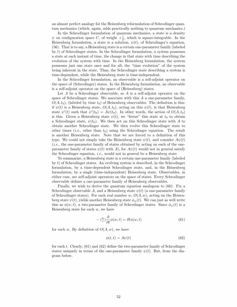
an almost perfect analogy for the Heisenberg reformulation of Schrodinger quan-tum mechanics (which, again, adds practically nothing to quantum mechanics.)

In the Schrodinger formulation of quantum mechanics, a state is a densityψ on configuration space C, of weight + 1

2 , which is square-integrable. In theHeisenberg formulation, a state is a solution, ψ(t), of Schrodinger’s equation,(56). That is to say, a Heisenberg state is a certain one-parameter family (labeledby t) of Schrodinger states. In the Schrodinger formulation, a system possessesa state at each instant of time, the change in that state with time describing theevolution of the system with time. In the Heisenberg formulation, the systempossesses just one state once and for all, the “time evolution” of the systembeing inherent in the state. Thus, the Schrodinger state describing a system istime-dependent, while the Heisenberg state is time-independent.

In the Schrodinger formulation, an observable is a self-adjoint operator onthe space of (Schrodinger) states. In the Heisenberg formulation, an observableis a self-adjoint operator on the space of (Heisenberg) states.

Let A be a Schrodinger observable, so A is a self-adjoint operator on thespace of Schrodinger states. We associate with this A a one-parameter family,O(A, t0), (labeled by time t0) of Heisenberg observables. The definition is this:if ψ(t) is a Heisenberg state, O(A, t0), acting on this ψ(t), is that Heisenbergstate ψ′(t) such that ψ′(t0) = Aψ(t0). In other words, the action of O(A, t0)is this. Given a Heisenberg state ψ(t), we “freeze” this state at t0 to obtaina Schrodinger state, ψ(t0). We then act on this Schrodinger state with A toobtain another Schrodinger state. We then evolve this Schrodinger state toother times (i.e., other than t0) using the Schrodinger equation. The resultis another Heisenberg state. Note that we are forced to a definition of thistype. We could not simply take the Heisenberg state ψ(t), and consider Aψ(t)(i.e., the one-parameter family of states obtained by acting on each of the one-parameter family of states ψ(t) with A), for Aψ(t) would not in general satisfythe Schrodinger equation, i.e., would not in general be a Heisenberg state.

To summarize, a Heisenberg state is a certain one-parameter family (labeledby t) of Schrodinger states. An evolving system is described, in the Schrodingerformulation, by a time-dependent Schrodinger state, and, in the Heisenbergformulation, by a single (time-independent) Heisenberg state. Observables, ineither case, are self-adjoint operators on the space of states. Every Schrodingerobservable defines a one-parameter family of Heisenberg observables.

Finally, we wish to derive the quantum equation analogous to (60). Fix aSchrodinger observable A, and a Heisenberg state ψ(t) (a one-parameter familyof Schrodinger states). For each real number w, O(A,w), acting on the Heisen-berg state ψ(t), yields another Heisenberg state φw(t). We can just as well writethis as φ(w, t), a two-parameter family of Schrodinger states. Since φw(t) is aHeisenberg state for each w, we have

− ( hi)

∂

∂tφ(w, t) = Hφ(w, t) (61)

for each w. By definition of O(A,w), we have

φ(t, t) = Aψ(t) (62)

for each t. Clearly, (61) and (62) define the two-parameter family of Schrodingerstates uniquely in terms of the one-parameter family ψ(t). But, from the dia-gram below,

52

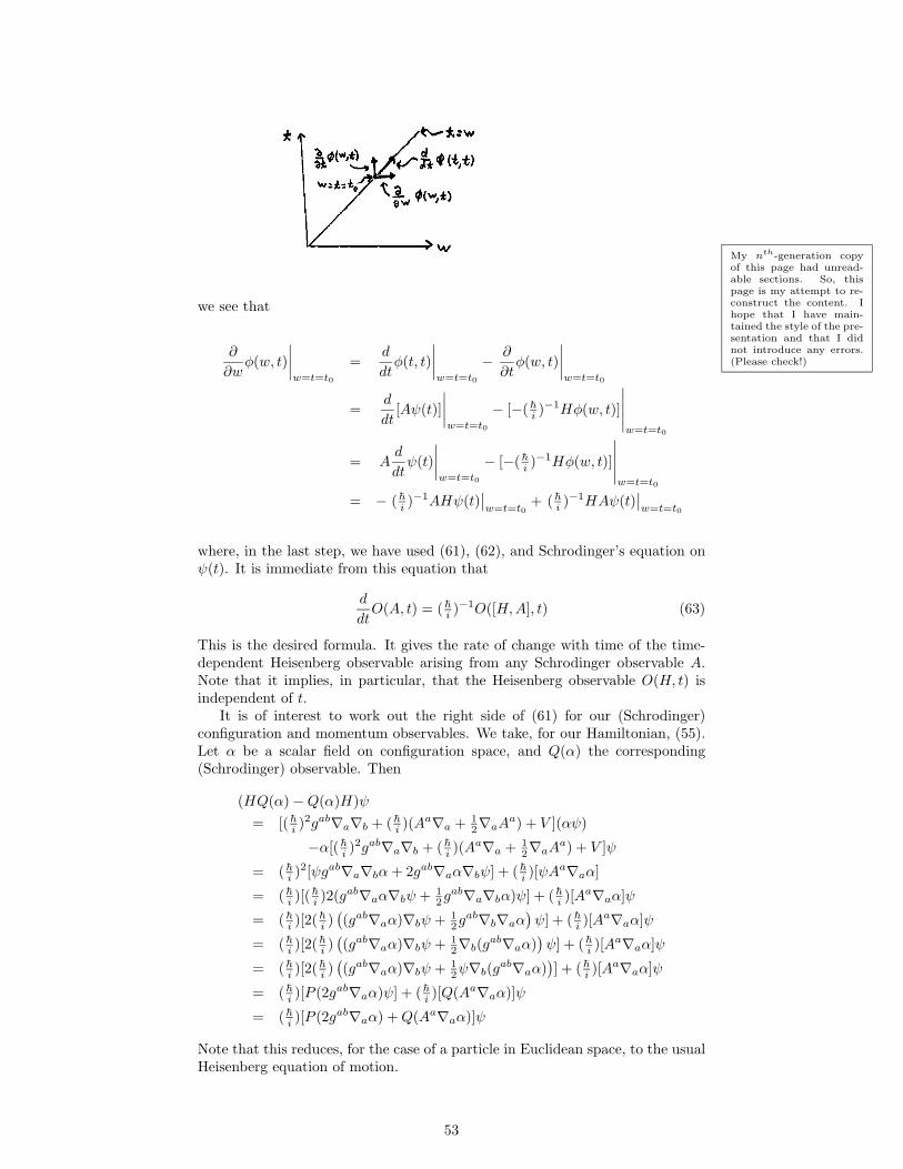
we see that

My nth-generation copyof this page had unread-able sections. So, thispage is my attempt to re-construct the content. Ihope that I have main-tained the style of the pre-sentation and that I didnot introduce any errors.(Please check!)

∂

∂wφ(w, t)

∣

∣

∣

∣

w=t=t0

=d

dtφ(t, t)

∣

∣

∣

∣

w=t=t0

−∂

∂tφ(w, t)

∣

∣

∣

∣

w=t=t0

=d

dt[Aψ(t)]

∣

∣

∣

∣

w=t=t0

− [−( hi)−1Hφ(w, t)]

∣

∣

∣

∣

∣

w=t=t0

= Ad

dtψ(t)

∣

∣

∣

∣

w=t=t0

− [−( hi)−1Hφ(w, t)]

∣

∣

∣

∣

∣

w=t=t0

= − ( hi)−1AHψ(t)

∣

∣

w=t=t0+ ( h

i)−1HAψ(t)

∣

∣

w=t=t0

where, in the last step, we have used (61), (62), and Schrodinger’s equation onψ(t). It is immediate from this equation that

d

dtO(A, t) = ( h

i)−1O([H,A], t) (63)

This is the desired formula. It gives the rate of change with time of the time-dependent Heisenberg observable arising from any Schrodinger observable A.Note that it implies, in particular, that the Heisenberg observable O(H, t) isindependent of t.

It is of interest to work out the right side of (61) for our (Schrodinger)configuration and momentum observables. We take, for our Hamiltonian, (55).Let α be a scalar field on configuration space, and Q(α) the corresponding(Schrodinger) observable. Then

(HQ(α) − Q(α)H)ψ

= [( hi)2gab∇a∇b + ( h

i)(Aa∇a + 1

2∇aAa) + V ](αψ)

−α[( hi)2gab∇a∇b + ( h

i)(Aa∇a + 1

2∇aAa) + V ]ψ

= ( hi)2[ψgab∇a∇bα + 2gab∇aα∇bψ] + ( h

i)[ψAa∇aα]

= ( hi)[( h

i)2(gab∇aα∇bψ + 1

2gab∇a∇bα)ψ] + ( hi)[Aa∇aα]ψ

= ( hi)[2( h

i)(

(gab∇aα)∇bψ + 12gab∇b∇aα

)

ψ] + ( hi)[Aa∇aα]ψ

= ( hi)[2( h

i)(

(gab∇aα)∇bψ + 12∇b(g

ab∇aα))

ψ] + ( hi)[Aa∇aα]ψ

= ( hi)[2( h

i)(

(gab∇aα)∇bψ + 12ψ∇b(g

ab∇aα))

] + ( hi)[Aa∇aα]ψ

= ( hi)[P (2gab∇aα)ψ] + ( h

i)[Q(Aa∇aα)]ψ

= ( hi)[P (2gab∇aα) + Q(Aa∇aα)]ψ

Note that this reduces, for the case of a particle in Euclidean space, to the usualHeisenberg equation of motion.

53

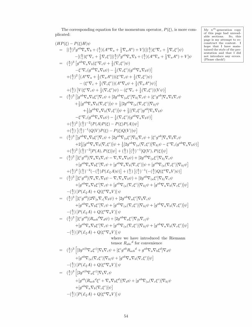
My nth-generation copyof this page had unread-able sections. So, thispage is my attempt to re-construct the content. Ihope that I have main-tained the style of the pre-sentation and that I didnot introduce any errors.(Please check!)

The corresponding equation for the momentum operator, P (ξ), is more com-plicated:

(HP (ξ) − P (ξ)H)ψ

= [( hi)2gab∇a∇b + ( h

i)(Aa∇a + 1

2∇aAa) + V ]([( hi)ξc∇c + 1

2∇cξc]ψ)

−[( hi)ξc∇c + 1

2∇cξc][( h

i)2gab∇a∇b + ( h

i)(Aa∇a + 1

2∇aAa) + V ]ψ

= ( hi)3

[

gab∇a∇b(ξc∇cψ + 1

2 (∇cξc)ψ)

−ξc∇c(gab∇a∇bψ) − 1

2 (∇cξc)(gab∇a∇bψ)

]

+( hi)2

[

(Aa∇a + 12 (∇aAa))(ξc∇cψ + 1

2 (∇cξc)ψ)

− (ξc∇c + 12 (∇cξ

c))(Aa∇aψ + 12 (∇aAa)ψ)

]

+( hi)[

V (ξc∇cψ + 12 (∇cξ

c)ψ) − (ξc∇c + 12 (∇cξ

c))(V ψ)]

= ( hi)3

[

[gab∇a∇bξc]∇cψ + [2gab∇(aξc]∇b)∇cψ + [ξcgab]∇a∇b∇cψ

+ 12 [gab∇a∇b(∇cξ

c)]ψ + 12 [2gab∇(a(∇cξ

c)]∇b)ψ

+ 12 [gab∇a∇b(∇cξ

c)]ψ + 12 [(∇cξ

c)gab]∇a∇bψ

−ξc∇c(gab∇a∇bψ) − 1

2 (∇cξc)(gab∇a∇bψ)

]

+( hi)2

[

( hi)−2(P (A)P (ξ) − P (ξ)P (A))ψ

]

+( hi)[

( hi)−1(Q(V )P (ξ) − P (ξ)Q(V ))ψ

]

= ( hi)3

[

[gab∇a∇bξc]∇cψ + [2gab∇(aξc]∇b)∇cψ + [ξcgab]∇a∇b∇cψ

+2 12 [gab∇a∇b(∇cξ

c)]ψ + 12 [2gab∇(a(∇cξ

c)]∇b)ψ − ξc∇c(gab∇a∇bψ)

]

+( hi)2

[

( hi)−2[P (A), P (ξ)]ψ

]

+ ( hi)[

( hi)−1[Q(V ), P (ξ)]ψ

]

= ( hi)3

[

[ξcgab](∇a∇b∇cψ −∇c∇a∇bψ) + [2gab∇(aξc]∇b)∇cψ

+[gab∇a∇bξc]∇cψ + [gab∇a∇b(∇cξ

c)]ψ + [gab∇(a(∇cξc)]∇b)ψ

]

+( hi)2

[

( hi)−2(−( h

i)P (£ξA)ψ)

]

+ ( hi)[

( hi)−1(−( h

i)Q(ξa∇aV )ψ)

]

= ( hi)3

[

[ξcgab](∇a∇c∇bψ −∇c∇a∇bψ) + [2gab∇(aξc]∇b)∇cψ

+[gab∇a∇bξc]∇cψ + [gab∇(a(∇cξ

c)]∇b)ψ + [gab∇a∇b(∇cξc)]ψ

]

−( hi) [P (£ξA) + Q(ξa∇aV )] ψ

= ( hi)3

[

[ξcgab](2∇[a∇c]∇bψ) + [2gab∇aξc]∇b∇cψ

+[gab∇a∇bξc]∇cψ + [gab∇(a(∇cξ

c)]∇b)ψ + [gab∇a∇b(∇cξc)]ψ

]

−( hi) [P (£ξA) + Q(ξa∇aV )] ψ

= ( hi)3

[

[ξcgab](Racbd∇dψ) + [2gab∇aξc]∇(b∇c)ψ

+[gab∇a∇bξc]∇cψ + [gab∇(a(∇cξ

c)]∇b)ψ + [gab∇a∇b(∇cξc)]ψ

]

−( hi) [P (£ξA) + Q(ξa∇aV )] ψ

where we have introduced the Riemanntensor Rabc

d for convenience

= ( hi)3

[

[2ga(b∇aξc)]∇b∇cψ + [ξcgabRacbd + gab∇a∇bξ

d]∇dψ

+[gab∇(a(∇cξc)]∇b)ψ + [gab∇a∇b(∇cξ

c)]ψ]

−( hi) [P (£ξA) + Q(ξa∇aV )] ψ

= ( hi)3

[

[2ga(b∇aξc)]∇b∇cψ

+[gab(Racbdξc + ∇a∇bξ

d)]∇dψ + [gab∇(a(∇cξc)]∇b)ψ

+[gab∇a∇b(∇cξc)]ψ

]

−( hi) [P (£ξA) + Q(ξa∇aV )] ψ

54

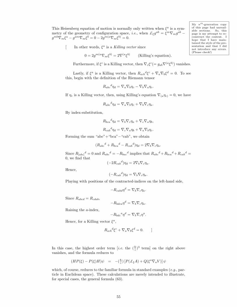
This Heisenberg equation of motion is normally only written when ξa is a sym-metry of the geometry of configuration space, i.e., when £ξg

ab = ξm∇mgab −gmb∇mξa − gam∇mξb = 0 − 2gm(a∇mξb) = 0.

My nth-generation copyof this page had unread-able sections. So, thispage is my attempt to re-construct the content. Ihope that I have main-tained the style of the pre-sentation and that I didnot introduce any errors.(Please check!)

[ In other words, ξa is a Killing vector since

0 = 2gm(a∇mξb) = 2∇(aξb) (Killing’s equation).

Furthermore, if ξc is a Killing vector, then ∇cξc(= gab∇

(aξb)) vanishes.

Lastly, if ξa is a Killing vector, then Racbdξc + ∇a∇bξ

d = 0. To seethis, begin with the definition of the Riemann tensor

Rabcdηd = ∇a∇bηc −∇b∇aηc.

If ηc is a Killing vector, then, using Killing’s equation ∇(aηc) = 0, we have

Rabcdηd = ∇a∇bηc + ∇b∇cηa.

By index-substitution,

Rbcadηd = ∇b∇cηa + ∇c∇aηb,

Rcabdηd = ∇c∇aηb + ∇a∇bηc.

Forming the sum “abc”+“bca”−“cab”, we obtain

(Rabcd + Rbca

d − Rcabd)ηd = 2∇b∇cηa.

Since R[abc]d = 0 and Rabc

d = −Rbacd implies that Rabc

d +Rbcad +Rcab

d =0, we find that

(−2Rcabd)ηd = 2∇b∇cηa.

Hence,(−Rcab

d)ηd = ∇b∇cηa.

Playing with positions of the contracted-indices on the left-hand side,

−Rcabdηd = ∇b∇cηa.

Since Rabcd = Rcdab,−Rbdcaηd = ∇b∇cηa.

Raising the a-index,−Rbdc

aηd = ∇b∇cηa.

Hence, for a Killing vector ξa,

Racbdξc + ∇a∇bξ

d = 0. ]

In this case, the highest order term [i.e. the ( hi)3 term] on the right above

vanishes, and the formula reduces to

(HP (ξ) − P (ξ)H)ψ = −( hi) [P (£ξA) + Q(ξa∇aV )] ψ

which, of course, reduces to the familiar formula in standard examples (e.g., par-ticle in Euclidean space). These calculations are merely intended to illustrate,for special cases, the general formula (63).

55

21. The Role of Observables. (Classical Me-chanics)

Our approach heretofore has been to introduce the states before the observ-ables. Thus, in classical mechanics, observables were functions on the space ofstates; in quantum mechanics, operators on the space of states—in both cases,observables were defined in terms of their relationship with states. It is naturalto proceed in this way, for one thinks of a system as possessing a state (indepen-dently of any observations which might be made on it), with the observationsrepresenting things which are applied to these states to give us informationabout the state. One could, however, imagine an alternative point of view. Onecould regard states, not as attributes of a system somehow handed down fromabove, but rather as something which must be determined by means of observa-tions. In other words, one could take a more observer-oriented point of view, inwhich the things which involve us observers directly—the observables—play thefundamental role. This point of view would be reflected within the mathemat-ical formulation by a formalism in which the observables are introduced as thefundamental objects, and the states only as subsidiary objects defined in termsof the observables. As an example, we first carry out such a reformulation forclassical mechanics.

We suppose that we are given some system to study. We have some mech-anism (e.g., hitting with a stick) by which we can cause our system to changestate, so we can experiment with various states. We are to be furnished, fur-thermore, with an enormous basket full of observables, where we think of anobservable as a box from which there protrudes a probe (which can be broughtin contact with the system), and which has a meter (which reads some valuewhen the system is in interaction with the observable). Our job is to introduce adescription of what is going on in terms of the meter readings of the observables.

One first, by trial and error, makes the following basic observation: if, to thesystem, observable A, then B, and then A are applied in quick succession (sothe system does not evolve appreciably between observables), then the readingsobtained for the two A observations coincide. We interpret this to mean thatthe application of our observables does not disturb the state of the system (i.e.,the application of B leaves invariant the A-reading, for all As, and hence leavesthe state alone). It follows that the application of several observables in quicksuccession is independent of the order in which the observables are applied.

Two observables, A and A′, will be said to be equivalent if they always givethe same result, applied to our system (more precisely, if the application of A

and A′ in quick succession yields the same reading on the two meters). We writeequivalence of observables with an equals sign.

We lose nothing in generality, yet simplify the discussion, by assuming thatour basket of observables has three properties. A constant observable is onewhose meter reading is always the same number (no matter what the systemis doing). We assume that, for each real number, there is in our collection ofobservables a constant observable which always yields that number. (If someconstant observable were missing from our collection, it would be easy to con-struct one to add to the collection. Just take an empty box, and paint on ita dial and needle always reading, for example, “3”.) Now let A and B be twoobservables. We define a new observable, obtained by applying A and B to thesystem in quick succession, and adding the readings on the two meters. Thisnew observable, called the sum of observables A and B, will be written A + B.Similarly, the product of two observables, AB, is another observable. We nowassume that our collection of observables contains, along with any two observ-ables, both their sum and their product. (If some sum, e.g., A+B, were missingfrom the collection, we could always construct, from A and B, A + B and addit to our collection). Note that addition and multiplication of observables sat-

56

isfy the same commutative, associative, and distributive laws that addition andmultiplication of real numbers do.

An algebra A is a vector space on which one or more bilinear products isdefined. (Thus, let A be a vector space on which products AB, A × B, and[A,B] are defined, satisfying (A+ cB)C = AC + cBC, A(B + cC) = AB + cAC,for c a number, and A, B, C in A, and similarly for the other two products.Then A is an algebra.)

The discussion above can now be summarized by the statement that wemight as well assume that our collection A of observables forms an algebra(with just one product, which is also associative and commutative).

A state is to be characterized in terms of what the observables have to sayabout it. That is to say, a state is a mapping σ : A → IR, from our algebra ofobservables to the reals, satisfying the following conditions:

1. If C is the constant observable with value c, then σ(C) = c.

2. If A and B are observables, then σ(A + B) = σ(A) + σ(B).

3. If A and B are observables, then σ(AB) = σ(A)σ(B).

These three conditions, of course, reflect the operational meaning of constantobservables, addition of observables, and multiplication of observables.

This is nearly the end of the story. From the algebra of observables, oneintroduces the states. We have still to ask, however, whether or not we obtain,in this way, the “correct” collection of states. The answer depends on whetheror not we have enough observables in our original collection A. For example,if A consisted of just the constant observables, then we would obtain, by theconstruction above, just one state. Suppose, however, that all observables wereincluded in our collection. Since we “really know” that our system has a phasespace, and the observables are scalar fields on phase space, this amounts to theassumption that for every scalar field on phase space there is an instrumentwhich measures that scalar field. We can then ask: does our construction aboveyield the correct collection of states? First note that every point of phase spacedoes indeed define a mapping from observables to the reals (namely, evaluationof the scalar field at the point). Hence, every point of phase space does definea state according to our construction. What needs to be shown is that noadditional states—no points of phase space—have been introduced. This is aconsequence of the following:

Theorem. Let M be a manifold, and let A be the algebra of scalar fields onM . Let σ : A → IR satisfy the three conditions above for a state. Then thereexists a point p of M such that σ(A) = A(p) for every A in A.

“proof”: the only proof I know requires the Whitney embedding theorem, astandard but rather technical result in differential geometry. Since a proof inthe special case M = IRn illustrates the essential idea, and since a proof inthis special case, together with the embedding theorem, yields easily a proof ingeneral, we shall assume M = IRn.

Let σ be a mapping as above, and consider the scalar fields x1, . . . , xn on M .Set x1 = σ(x1), . . . , xn = σ(xn). Let p the point with coordinates (x1, . . . , xn).Then, for f any scalar field on M , we can write f = f + f1(x

1 − x1) + · · · +

fn(xn − xn), where f is a constant scalar field, and f1, . . . , fn are scalar fields.

Then σ(f) = σ(f) + σ(f1)(σ(x1)− σ(x1)) + · · ·+ σ(fn)(σ(xn)− σ(xn)) = σ(f),

where, in the last step, we have used that σ(xi) = xi = σ(xi). Thus, σ(f) =σ(f) = f = f(p), completing the proof.

Thus, if we have all the observables in our original collection, we can con-struct the space of states as above, and indeed obtain precisely the correct spaceof states. A similar conclusion holds even if original algebra includes fewer ob-servables. For example, it easy to check, using the same methods above, that,

57

if A is the algebra of algebraic observables, then we obtain the correct space ofstates. Note, furthermore, that, if A includes all the configuration and momen-tum observables, then, since A is an algebra, A necessarily includes all algebraicobservables. Then, so long as A includes all configuration and momentum ob-servables, precisely the correct space of states emerges from the constructionabove.

58

22. The Role of Observables. (Quantum Me-chanics)

Ideally, one would now like to repeat, for quantum mechanics, what we didin the previous section for classical mechanics. That is to say, one would liketo introduce a collection of observables (measuring instruments) on a quantumsystem, subject to some physically reasonably conditions regarding the action ofthe instruments on the system, and then define the states in terms of the observ-ables. In this way, one might expect both to obtain a more operational settingfor quantum mechanics, and to provide more direct physical interpretations forcertain objects which appear in the mathematical formalism of quantum me-chanics. It appears, however, that certain difficulties intervene to prevent asimple and direct treatment of quantum mechanics along these lines. In thissection, we discuss these difficulties.

We must first consider the mechanism by which observables act on states.Within the formalism of quantum mechanics, an observable is a self-adjointoperator on the space of states. What we must do is relate the mathematicalaction of this operator to the physical action of the observing instrument on thestate. There are, apparently, two possible such relationships.

1. Active observables. One wishes to apply to the state the observable as-sociated with the self-adjoint operator A. The meter on the instrumentreads an eigenvalue of A, i.e., a number such that Aψ = aψ for somenonzero state ψ. During the observation, the system suddenly changes itsstate so that, after an observation yielding the value a, the system is inthe corresponding eigenstate (i.e., the ψ above). Even though the initialstate ψ, as well as the self-adjoint operator A, are known, the final stateinto which the system passes is not uniquely determined. Rather, what isdetermined is the probabilities for the various eigenvalue-eigenstate pairs.

2. Passive observables. The application, to the state ψ, of the observableassociated with the self-adjoint operator A yields (as the reading of theinstrument) the expectation value of A in our state, i.e., the real number〈ψ |Aψ 〉. The effect of this measurement on the state of the system canbe made arbitrarily small.

I believe that it is true to say that, given A, one can construct measuringinstruments, of either the active or the passive type, corresponding to A. Themeasuring instruments we introduced in classical mechanics were passive, al-though one could, of course, have introduced also active instruments (whichwould change the state of the system). Of course, one could, if it should turnout to be convenient, simply require that the instrument he uses be of one orthe other type. In particular, one often treats quantum mechanics using onlyactive instruments. The possibilities for defining states in terms of observablesdepend on which type of observing instruments one chooses to use. We shallconsider the results of using both types.

The disadvantage of using active instruments is that they interfere, in asignificant and uncontrollable way, with the state being observed. In fact, theoriginal state is for all practical purposes destroyed by the making of a singleactive observation. However, a vestige of the original does survive in that theoriginal state determines the probability distribution for the various possibleeigenvalues which could emerge from the observation. Unfortunately, a singleobservation on a single system yields, not a probability distribution, but a singleeigenvalue. It is clearly impossible to describe a state in terms of observations onthat state in the presence of this strong interference of the observing instrumentwith state itself.

There is, however, a method for avoiding at least certain of these difficulties.Let us imagine that we have been given a method for preparing the system so

59

as to be in a given state. We then make up an infinite collection of copies of ouroriginal of copies of our original system, all in the same state. This collectionis called an ensemble. One now imagines applying observing instruments, notto a single system (in the single state), but to an ensemble. This is done bymaking the observation on some infinite sub-collection of the systems formingthe ensemble, leaving, at the same time, an infinite collection of systems in theensemble unobserved. (For example, one could observe every other system inthe ensemble.) For each system observed, one records the number (eigenvalue)determined by the observing instrument. The observed systems can then bediscarded (their states having been ruined). There remains, however, an infi-nite collection of systems which have not been disturbed, i.e., an ensemble forfurther study. Thus, by introducing ensembles rather than states, one avoidsthe difficulties associated with the interference of observations with the state ofthe system. One must pay for this device, however, in that one must, in a sense,already know what the states are, for, to prepare an ensemble, one must havein hand a repeatable prescription for putting the system in a given state.

In any case, the information we obtain by applying an observable to anensemble is a probability measure on the real line (i.e., a positive measure suchthat the total measure of the line is one).

Thus, one would attempt to proceed as follows. One would introduce analgebra of (active) observables. States would be defined as mappings from thisalgebra to probability measures on the real line, such that the mapping satisfycertain conditions. One would then have to show that the correct space ofstates is obtained in this way. Unfortunately, it appears to be very difficult tomake such a program work, in the sense that one finds suitable structure onthe observables and suitable additional conditions for the definition of a state,such that the structure and conditions can be motivated physically, and suchthat the resulting collection of states agrees with the space of states of quantummechanics.

It is perhaps not too surprising that the use of active observables shouldlead to difficulties. The program of defining states in terms of observables worksextremely well in classical mechanics, and in that case the observables are inevery sense passive. One would naturally expect that the passive observableswould be the most natural to use also in quantum mechanics.

Let us attempt, then, to describe states in terms of expectation values forself-adjoint operators, i.e., in terms of passive observables. It is perhaps notunreasonable to ask that included in our collection of observables be all config-uration and momentum observables. We begin with a mathematical question:does knowledge of the numbers 〈ψ |Q(α)ψ 〉 and 〈ψ |P (ξ)ψ 〉 for all α and ξa

determine ψ? If not, our goal is hopeless; if so, we can ask how this determi-nation comes about. Set ψ = φeiλ, where φ and λ are real scalar fields. (Forsimplicity, we take ψ as a scalar field.) Then

〈ψ |Q(α)ψ 〉 =

∫

(φeiλ)αφeiλ =

∫

φ2α (64)

〈ψ |P (ξ)ψ 〉 =

∫

(φeiλ)( hi)(ξa∇a + 1

2∇aξa)φeiλ

=

∫

( hi)φe−iλ(eiλξa∇aφ + iφeiλξa∇aλ + 1

2φeiλ∇aξa)

=

∫

( hi)φξa∇aφ +

∫

hφ2ξa∇aλ +

∫

12 ( h

i)φ2∇aξa

=

∫

12 ( h

i)(2φξa∇aφ + φ2∇aξa) +

∫

hφ2ξa∇aλ

=

∫

12 ( h

i)∇a(φ2ξa) +

∫

hφ2ξa∇aλ

60

=

∫

hφ2ξa∇aλ

= h〈ψ |Q(ξa∇aλ)ψ 〉 (65)

Knowledge of the expectation value of Q(α) for all α determines, by (64), φ.Then the expectation value of P (ξ) for all ξa determines, by (65), ∇aλ, andhence λ up to a constant. Thus, ψ = φeiλ is determined up to an overall phase(which is all the wave function is ever determined up to, anyway). Our programshould, in principle, succeed.

Denote by Q the collection of all (passive) configuration observables, andby P the collection of all (passive) momentum observables. One knows, opera-tionally, how to multiply an element of Q or an element of P by a real number,and how to add two elements of Q or two elements of P. Thus, each of Q, Phas the structure of a vector space. A state is to consist of linear mappingsσ : Q → IR and σ : P → IR. We wish to impose additional conditions on thesemappings in order that σ(α) = 〈ψ |Q(α)ψ 〉 and σ(ξ) = 〈ψ |P (ξ)ψ 〉 for somestate ψ. It follows from the linearity of σ that there exist scalar and vector fieldsµ and µa on configuration space such that

σ(α) =

∫

αµ (66)

σ(ξ) =

∫

ξaµa (67)

for all α and ξa. (We should, more precisely, allow µ and µa to be distributionson configuration space. Thus, for example, a scalar distribution is normallydefined as a linear mapping from scalar fields on a manifold to reals. In orderto avoid technical complications, however, we shall restrict consideration to thecase when µ and µa are ordinary tensor fields.) We wish to define φ by φ2 = µ,and for this we need µ ≥ 0. We can state this condition in terms of our operatorsas follows: if α ≥ 0, then σ(α) ≥ 0. We wish to define λ by hφ2∇aλ = µa,which requires that φ−2µa be a gradient. This condition is equivalent to therequirement that, whenever ξa is such that ∇a(φ2ξa) = 0, σ(ξ) = 0, i.e., to therequirement that whenever ξa is such that σ(ξa∇aα) = 0 for all α, σ(ξ) = 0.With these two conditions, we can recover φ and λ, and hence the state ψ = φeiλ,from the mappings σ.

To summarize, we introduce two vector spaces, Q and P, of observables. Astate is then defined as a pair of linear mappings, σ : Q → IR and σ : P → IR,satisfying two conditions:

1. If α ≥ 0, then σ(α) ≥ 0.

2. If σ(ξa∇aα) = 0 for all α, then σ(ξ) = 0.

Then, roughly speaking, for every such state there is a unique wave functionψ on configuration space such that σ(α) =

∫

ψαψ and σ(ξ) =∫

ψ( hi)(ξa∇a +

12∇aξa)ψ.

Note that our two conditions in the definition of a state are indeed satisfiedin the classical case. (Classically, the second condition amounts essentially tothe statement that vector fields are defined as derivations on scalar fields, so thezero derivation defines the zero vector field). Why were we able to avoid explicitmention of such conditions in the classical case? The reason is that we were ablethere to introduce a far stronger condition in the definition of states, namely,the product condition: σ(AB) = σ(A)σ(B). One might imagine, therefore,that matters could be simplified in the quantum case by the introduction ofa similar product condition. Of course, it is easy, operationally, to introducethe product of two (passive, quantum) observables. Given instruments whichmeasure A and B, one constructs an instrument which measures first A andthen B, and multiplies. (Since passive observables do not affect the states, this

61

construction is independent of order.) The difficulty, however, is this: if A andB are self-adjoint operators, then, in general,

〈ψ |Aψ 〉〈ψ |Bψ 〉 6= ψABψ (68)

The left hand side is the number associated with the “product observable” con-structed above. The right side is the expectation value associated with theproduct of operators. In short, the operational procedure of taking products ofobservables does not correspond to the mathematical procedure of taking prod-ucts of operators. The incorporation of operational products into our quantumobservables thus adds essentially nothing new.

Thus, we indeed obtain a formulation of quantum mechanics in which statesare described in terms of (passive) observables. Although the two conditions werequire in the definition of a state (that σ(α) ≥ 0 if α ≥ 0, and that σ(ξ) = 0if σ(ξa∇aα) = 0 for all α) are perhaps not terribly unnatural physically, thesecond certainly seems rather artificial. One could easily invent other conditionsof the same general type which are not imposed. There is, however, another—perhaps even more unpleasant—feature of this formulation. In the classical case,we could think of our observables as measuring instruments, instruments whichwe knew how to apply to our system, but about which no further informationwas required. This is not at all the case for our quantum observables. Firstly, weneed to know which instruments measure configuration and which momentumobservables. That is to say, each instrument must have, inscribed on its side,either “Q” or “P”. In fact, we need, for the construction of states above, muchmore than this. We also need to know, for each instrument which measuresa configuration observable, which scalar field α on configuration space this in-strument measures (the expectation value of), and, for each instrument whichmeasures a momentum observable, which vector field ξa is observed. This ad-ditional information is necessary in order that the construction of states can becarried out. On the other hand, no operational procedure is given for obtainingthis additional information, e.g., no procedure for discovering what an instru-ment measures by taking it apart. In fact, the introduction of such observablesrequires already a knowledge of what configuration space is—but configurationspace determines already the quantum states.

To summarize, because the measurement process in quantum mechanics isapparently more subtle than that in classical mechanics, the simple formulationof classical mechanics in terms of observables apparently does not carry over ina natural and equally simple way into quantum mechanics.

62

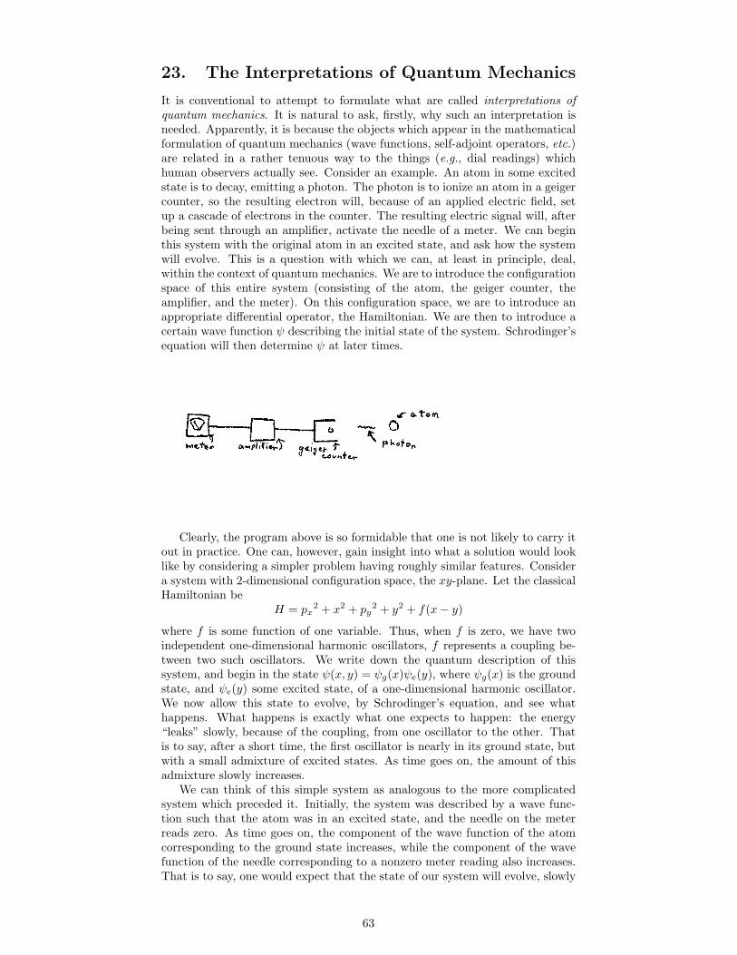
23. The Interpretations of Quantum Mechanics

It is conventional to attempt to formulate what are called interpretations ofquantum mechanics. It is natural to ask, firstly, why such an interpretation isneeded. Apparently, it is because the objects which appear in the mathematicalformulation of quantum mechanics (wave functions, self-adjoint operators, etc.)are related in a rather tenuous way to the things (e.g., dial readings) whichhuman observers actually see. Consider an example. An atom in some excitedstate is to decay, emitting a photon. The photon is to ionize an atom in a geigercounter, so the resulting electron will, because of an applied electric field, setup a cascade of electrons in the counter. The resulting electric signal will, afterbeing sent through an amplifier, activate the needle of a meter. We can beginthis system with the original atom in an excited state, and ask how the systemwill evolve. This is a question with which we can, at least in principle, deal,within the context of quantum mechanics. We are to introduce the configurationspace of this entire system (consisting of the atom, the geiger counter, theamplifier, and the meter). On this configuration space, we are to introduce anappropriate differential operator, the Hamiltonian. We are then to introduce acertain wave function ψ describing the initial state of the system. Schrodinger’sequation will then determine ψ at later times.

Clearly, the program above is so formidable that one is not likely to carry itout in practice. One can, however, gain insight into what a solution would looklike by considering a simpler problem having roughly similar features. Considera system with 2-dimensional configuration space, the xy-plane. Let the classicalHamiltonian be

H = px2 + x2 + py

2 + y2 + f(x − y)

where f is some function of one variable. Thus, when f is zero, we have twoindependent one-dimensional harmonic oscillators, f represents a coupling be-tween two such oscillators. We write down the quantum description of thissystem, and begin in the state ψ(x, y) = ψg(x)ψe(y), where ψg(x) is the groundstate, and ψe(y) some excited state, of a one-dimensional harmonic oscillator.We now allow this state to evolve, by Schrodinger’s equation, and see whathappens. What happens is exactly what one expects to happen: the energy“leaks” slowly, because of the coupling, from one oscillator to the other. Thatis to say, after a short time, the first oscillator is nearly in its ground state, butwith a small admixture of excited states. As time goes on, the amount of thisadmixture slowly increases.

We can think of this simple system as analogous to the more complicatedsystem which preceded it. Initially, the system was described by a wave func-tion such that the atom was in an excited state, and the needle on the meterreads zero. As time goes on, the component of the wave function of the atomcorresponding to the ground state increases, while the component of the wavefunction of the needle corresponding to a nonzero meter reading also increases.That is to say, one would expect that the state of our system will evolve, slowly

63

and continuously, from one in which the atom is excited and the meter readszero, to one in which the atom has decayed and the meter reads nonzero.

On the other hand, one can actually buy, e.g., from Sears, a geiger counter,amplifier, meter, and excited atom. One sets up the experiment, and watchesthe needle as the system evolves. What one actually sees, of course, is that theneedle remains at zero for a while, then jumps to some value. One often saysthat, at the instant the needle jumped, the atom decayed, and the photon wasreceived by the geiger counter, amplified, and recorded by the meter.

We now have two descriptions of this experiment. In one, via the formalismof quantum mechanics, the wave function of the needle continuously evolves fromthat corresponding to a zero reading to that corresponding to a finite reading.In the other, via direct observation, the needle is seen, not in some “smeared outstate”, half reading zero and half something else, but is rather seen to remain atzero for a while then jump suddenly. The problem of interpretation, as it bearson this example, is to somehow bring together these two descriptions. Thatis to say, the problem of interpretation is to make more sharp the relationshipbetween the objects which appear in the formalism of quantum mechanics andthe things observers actually see.

It is not at all uncommon in physics (perhaps it is even characteristic!)that the objects at the center of the mathematical description are not thefirst and most obvious things observers see. Special relativity is a good ex-ample. Fundamental in the mathematical description of special relativity arethe events (instantaneous occurrences at a point), which are assembled into thefour-dimensional space-time manifold. Yet, although each of us lives (ignoringgravity) in the four-dimensional space-time manifold of special relativity, we donot experience any four-dimensional manifold stretching out before us. Instead,we experience three-dimensional space, and the passage of time. Why, then,does one not feel a need to acquire an “interpretation” of special relativity?

It is my impression that an interpretation is as necessary in special relativityas in quantum mechanics, but that, in the case of the former, an interpretationis available and widely accepted, so that its role as an interpretation normallygoes unemphasized. This interpretation is that each of us (our past, present, andfuture) is represented by a world-line in space-time, that what we experience islight rays reaching our world-line from distant events, objects whose world-linesmeet ours, etc. Within this framework—a framework in which the observer isincorporated directly—one can, in some sense, account for what we as observersactually see.

It is perhaps not the whole truth to say that those experiences for whichspecial relativity might give account are in fact accounted for by special rela-tivity. It is, for example, not so easy to account, within special relativity, forthe fact that one cannot go back and actively experience his past. However,one perhaps takes the point of view that these finer details are somehow to bedescribed in terms of the detailed physics of what goes on in the brain. Onemight also say, based on this discussion of special relativity, that the purposeof an interpretation is, not really to explain anything, but rather to put one atease while he works within the mathematical formalism.

We return to quantum mechanics. As discussed above, there is a sense inwhich quantum mechanics is inadequate. On the other hand, there is certainlya sense in which quantum mechanics is far more than adequate: it makes beau-tiful and accurate predictions in remarkable agreement with Nature. One wouldtherefore not like to change in a substantive way the structure of quantum me-chanics, e.g., change its mathematical formalism. What one would like to do isto look at quantum mechanics from a different point of view, or at least uttersome reassuring words about it, so that the apparent inadequacy seems lessserious. That is to say, what one would like to do is formulate an interpretationof quantum mechanics.

64

24. The Copenhagen Interpretation

The most widely accepted interpretation of quantum mechanics is what is calledthe Copenhagen interpretation.

The idea of the Copenhagen interpretation, as I understand it, is that quan-tum mechanics is fine as far as it goes, but that it does not go far enough. Whatis missing is the relationship between the wave function and what observers see.The Copenhagen interpretation attempts to provide this additional link.

One first notices that, if you ask an observer what it was that he actually saw,he will say “I saw the meter read 3.5.”, or “I saw the light go on.”, but never “Thewave function of the needle on the meter was the following superposition...”.Thus, this additional link is to somehow tie together quantum phenomena (i.e.,wave functions) and classical phenomena (i.e., points of configuration space).

Consider again the experiment on page 63. We wish to regard the meterclassically, and the original atom quantum mechanically. We therefore intro-duce a break at some point between the chain of instruments linking the atomto the meter, e.g., between the atom and the geiger counter. Everything upto the break (in the case, just the atom itself) will be treated quantum me-chanically, and everything beyond the break (in this case, the geiger counter,amplifier, and meter) will be treated classically. Put more formally, we intro-duce a classical phase space to describe the states of the meter-amplifier-geigercounter system, and a space of quantum states (i.e., complex functions on anappropriate configuration space) to describe the original atom.

The next step is to introduce a coupling of these two systems, across thebreak. This is done by assigning a self-adjoint operator A to the quantumsystem, and, at the same time, assigning a state of the classical system toeach eigenvalue of A. The prescription for making these assignments is notspecified by the interpretation, but the assignments are to be so made that, inthe end, one obtains an appropriate description of this measurement process.The essential assumption is that one can introduce a break in this chain ofinstruments, and describe the information flow across the break in terms ofa self-adjoint operator A on the quantum system, and states of the classicalsystem labeled by eigenvalues of A.

The break comes into play during what is called process of measurement.The following then takes place. The Schrodinger equation for the quantumsystem, and the Hamilton equation for the classical system are, for a moment,suspended. During this suspension the quantum system is thrown into an eigen-state of A, and, simultaneously, the classical system is thrown into the stateassociated with the corresponding eigenvalue of A. The process of measurementis thus a process of sudden change in state. In this way, the formalism of quan-tum mechanics is to be brought into contact with the (classical) things people,as observers, see.

The particular eigenstate of A into which the quantum state is thrown duringthe process of measurement is not specified precisely. Rather, what can bedetermined is the probability distribution for various of the probabilities. Thus,there is, in a sense, a loss of determinism in the Copenhagen interpretation,associated with the process of measurement. It is essentially at this point thatprobability is brought into quantum mechanics.

One might object to the interpretation above on, among others, the follow-ing grounds. No prescription has been given for where to introduce the breakbetween the quantum and classical systems. Thus, in our example, one could aswell have drawn the break between the geiger counter and amplifier, or betweenthe amplifier and meter. It is, so I understand, part of the lore of the Copen-hagen interpretation that the result (i.e., the resulting probability distributionfor the meter readings) is independent of this choice. It is not completely clearhow one formulates a precise statement along these lines, although indicationsare (e.g., from simple examples) that something of this general type is true.

65

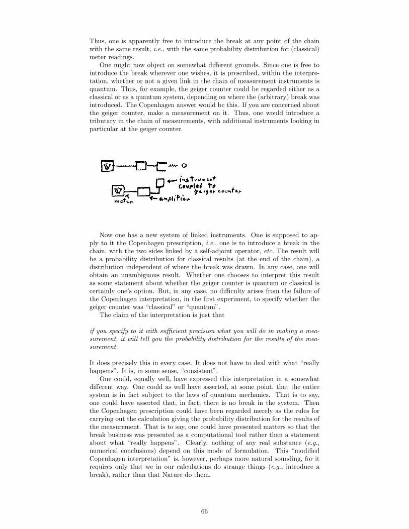
Thus, one is apparently free to introduce the break at any point of the chainwith the same result, i.e., with the same probability distribution for (classical)meter readings.

One might now object on somewhat different grounds. Since one is free tointroduce the break wherever one wishes, it is prescribed, within the interpre-tation, whether or not a given link in the chain of measurement instruments isquantum. Thus, for example, the geiger counter could be regarded either as aclassical or as a quantum system, depending on where the (arbitrary) break wasintroduced. The Copenhagen answer would be this. If you are concerned aboutthe geiger counter, make a measurement on it. Thus, one would introduce atributary in the chain of measurements, with additional instruments looking inparticular at the geiger counter.

Now one has a new system of linked instruments. One is supposed to ap-ply to it the Copenhagen prescription, i.e., one is to introduce a break in thechain, with the two sides linked by a self-adjoint operator, etc. The result willbe a probability distribution for classical results (at the end of the chain), adistribution independent of where the break was drawn. In any case, one willobtain an unambiguous result. Whether one chooses to interpret this resultas some statement about whether the geiger counter is quantum or classical iscertainly one’s option. But, in any case, no difficulty arises from the failure ofthe Copenhagen interpretation, in the first experiment, to specify whether thegeiger counter was “classical” or “quantum”.

The claim of the interpretation is just that

if you specify to it with sufficient precision what you will do in making a mea-surement, it will tell you the probability distribution for the results of the mea-surement.

It does precisely this in every case. It does not have to deal with what “reallyhappens”. It is, in some sense, “consistent”.

One could, equally well, have expressed this interpretation in a somewhatdifferent way. One could as well have asserted, at some point, that the entiresystem is in fact subject to the laws of quantum mechanics. That is to say,one could have asserted that, in fact, there is no break in the system. Thenthe Copenhagen prescription could have been regarded merely as the rules forcarrying out the calculation giving the probability distribution for the results ofthe measurement. That is to say, one could have presented matters so that thebreak business was presented as a computational tool rather than a statementabout what “really happens”. Clearly, nothing of any real substance (e.g.,numerical conclusions) depend on this mode of formulation. This “modifiedCopenhagen interpretation” is, however, perhaps more natural sounding, for itrequires only that we in our calculations do strange things (e.g., introduce abreak), rather than that Nature do them.

66

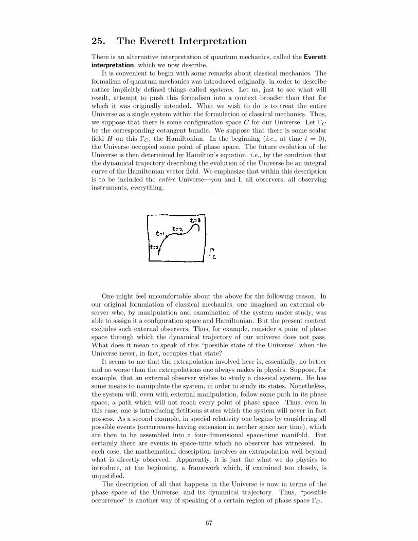
25. The Everett Interpretation

There is an alternative interpretation of quantum mechanics, called the Everett

interpretation, which we now describe.It is convenient to begin with some remarks about classical mechanics. The

formalism of quantum mechanics was introduced originally, in order to describerather implicitly defined things called systems. Let us, just to see what willresult, attempt to push this formalism into a context broader than that forwhich it was originally intended. What we wish to do is to treat the entireUniverse as a single system within the formulation of classical mechanics. Thus,we suppose that there is some configuration space C for our Universe. Let ΓC

be the corresponding cotangent bundle. We suppose that there is some scalarfield H on this ΓC , the Hamiltonian. In the beginning (i.e., at time t = 0),the Universe occupied some point of phase space. The future evolution of theUniverse is then determined by Hamilton’s equation, i.e., by the condition thatthe dynamical trajectory describing the evolution of the Universe be an integralcurve of the Hamiltonian vector field. We emphasize that within this descriptionis to be included the entire Universe—you and I, all observers, all observinginstruments, everything.

One might feel uncomfortable about the above for the following reason. Inour original formulation of classical mechanics, one imagined an external ob-server who, by manipulation and examination of the system under study, wasable to assign it a configuration space and Hamiltonian. But the present contextexcludes such external observers. Thus, for example, consider a point of phasespace through which the dynamical trajectory of our universe does not pass.What does it mean to speak of this “possible state of the Universe” when theUniverse never, in fact, occupies that state?

It seems to me that the extrapolation involved here is, essentially, no betterand no worse than the extrapolations one always makes in physics. Suppose, forexample, that an external observer wishes to study a classical system. He hassome means to manipulate the system, in order to study its states. Nonetheless,the system will, even with external manipulation, follow some path in its phasespace, a path which will not reach every point of phase space. Thus, even inthis case, one is introducing fictitious states which the system will never in factpossess. As a second example, in special relativity one begins by considering allpossible events (occurrences having extension in neither space nor time), whichare then to be assembled into a four-dimensional space-time manifold. Butcertainly there are events in space-time which no observer has witnessed. Ineach case, the mathematical description involves an extrapolation well beyondwhat is directly observed. Apparently, it is just the what we do physics tointroduce, at the beginning, a framework which, if examined too closely, isunjustified.

The description of all that happens in the Universe is now in terms of thephase space of the Universe, and its dynamical trajectory. Thus, “possibleoccurrence” is another way of speaking of a certain region of phase space ΓC .

67

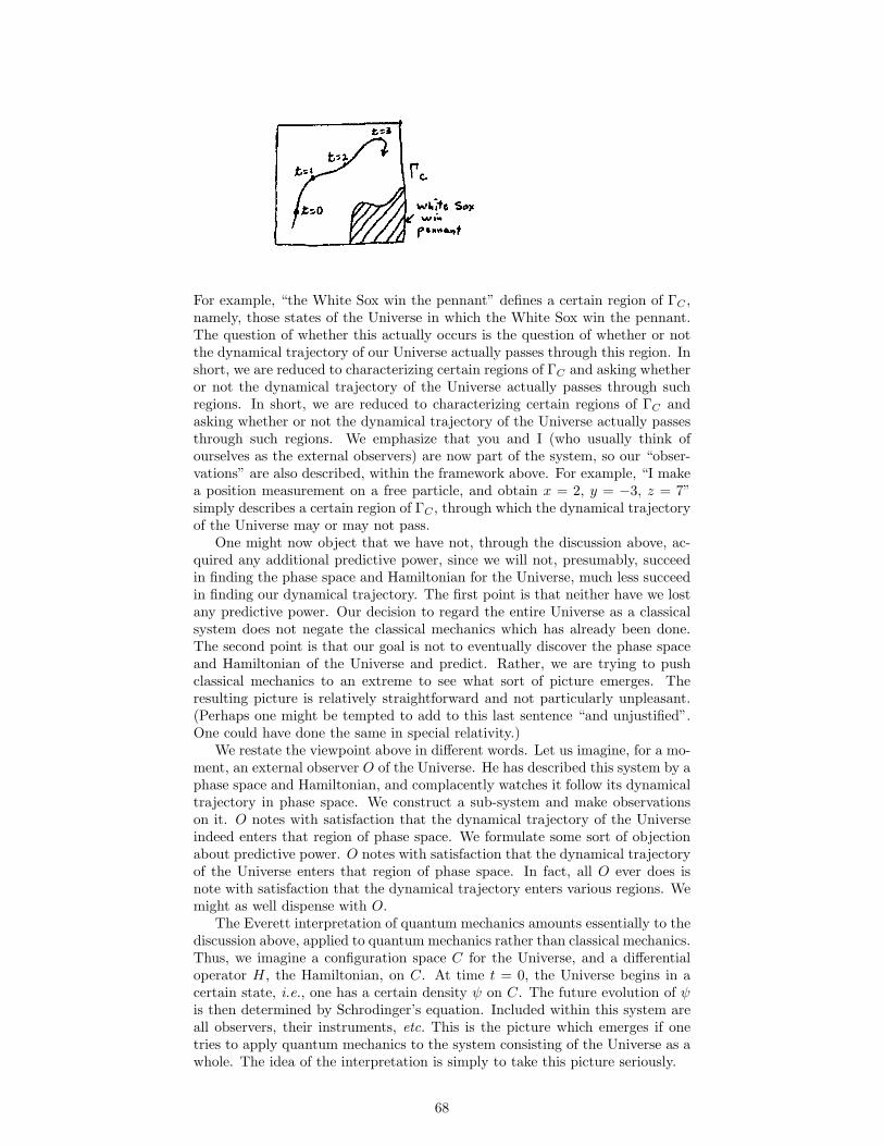
For example, “the White Sox win the pennant” defines a certain region of ΓC ,namely, those states of the Universe in which the White Sox win the pennant.The question of whether this actually occurs is the question of whether or notthe dynamical trajectory of our Universe actually passes through this region. Inshort, we are reduced to characterizing certain regions of ΓC and asking whetheror not the dynamical trajectory of the Universe actually passes through suchregions. In short, we are reduced to characterizing certain regions of ΓC andasking whether or not the dynamical trajectory of the Universe actually passesthrough such regions. We emphasize that you and I (who usually think ofourselves as the external observers) are now part of the system, so our “obser-vations” are also described, within the framework above. For example, “I makea position measurement on a free particle, and obtain x = 2, y = −3, z = 7”simply describes a certain region of ΓC , through which the dynamical trajectoryof the Universe may or may not pass.

One might now object that we have not, through the discussion above, ac-quired any additional predictive power, since we will not, presumably, succeedin finding the phase space and Hamiltonian for the Universe, much less succeedin finding our dynamical trajectory. The first point is that neither have we lostany predictive power. Our decision to regard the entire Universe as a classicalsystem does not negate the classical mechanics which has already been done.The second point is that our goal is not to eventually discover the phase spaceand Hamiltonian of the Universe and predict. Rather, we are trying to pushclassical mechanics to an extreme to see what sort of picture emerges. Theresulting picture is relatively straightforward and not particularly unpleasant.(Perhaps one might be tempted to add to this last sentence “and unjustified”.One could have done the same in special relativity.)

We restate the viewpoint above in different words. Let us imagine, for a mo-ment, an external observer O of the Universe. He has described this system by aphase space and Hamiltonian, and complacently watches it follow its dynamicaltrajectory in phase space. We construct a sub-system and make observationson it. O notes with satisfaction that the dynamical trajectory of the Universeindeed enters that region of phase space. We formulate some sort of objectionabout predictive power. O notes with satisfaction that the dynamical trajectoryof the Universe enters that region of phase space. In fact, all O ever does isnote with satisfaction that the dynamical trajectory enters various regions. Wemight as well dispense with O.

The Everett interpretation of quantum mechanics amounts essentially to thediscussion above, applied to quantum mechanics rather than classical mechanics.Thus, we imagine a configuration space C for the Universe, and a differentialoperator H, the Hamiltonian, on C. At time t = 0, the Universe begins in acertain state, i.e., one has a certain density ψ on C. The future evolution of ψ

is then determined by Schrodinger’s equation. Included within this system areall observers, their instruments, etc. This is the picture which emerges if onetries to apply quantum mechanics to the system consisting of the Universe as awhole. The idea of the interpretation is simply to take this picture seriously.

68

When referring to a system, one speaks of something happening in thatsystem, one normally means that some classical possibility has been realized.Suppose we watch a quantum system consisting of a geiger counter and atom,such that the photon resulting from the decay of the atom would be registered bythe geiger counter. Our description of this system would be by a wave functionwhich evolves by Schrodinger’s equation. The wave function may, as it evolves,become large or small for certain classical possibilities (i.e., in certain regionsof configuration space), but nothing ever “happens” in the classical sense. Thescheme above requires that we regard the Universe as a quantum system. Thus,from this viewpoint, nothing “happens” in the Universe (in the sense that noclassical possibilities are actually realized). In other words, since implicit inquantum mechanics is a wave function rather than the occurrence of classicalpossibilities, we are forced, if we are to regard the Universe as a quantum system,to deny the occurrence, in the Universe, of classical possibilities.

One might object, at this point, that this denial is in disagreement with oureveryday observations. We, apparently, do see classical possibilities “occur”. Ifwe watch the meter attached to the geiger counter, we do see, at some point,the needle jump. The response to this objection, from the present point ofview, is that this impression of ours is simply another manifestation of thewave function of the Universe. Suppose that we, as observers, were watchinga quantum system consisting of some rabbits, who have geiger counters andatoms, and who do various experiments. The rabbits may indeed formulatesome sort of quantum theory in which classical possibilities seem to actuallyoccur. We, however, would describe this system quite differently. We wouldsay that there is an evolving wave function on the configuration space of thesystem. Whatever impressions the rabbits get would simply be a manifestationof that wave function. Thus, from the present viewpoint, we regard our everydayimpression that classical possibilities actually occur as being a manifestation ofthe wave function of the Universe.

One could now formulate a second objection, that our impression that clas-sical possibilities actually occur is not being explained by this framework, in thesense that we are not shown in detail how this impression is represented by thewave function of the Universe. The point is that this is something we will not beable to explain without a great deal more information about how Humans areconstructed. But this is perhaps not so unpleasant, for there are many everydayhuman impressions which are not adequately described by physics, presumablybecause of a lack of information about the workings of people.

For example, we all observe that we cannot go back and actively re-liveour pasts. This observation presumably falls under special relativity. Yet itis difficult to construct some theorem in special relativity which reflects thisobservation. Our understanding of this everyday observation would presumablyimprove if we understood better the internal workings of people. Yet, one canget along quite well in special relativity without such an understanding. Asimilar point is to be made within the Everett interpretation. That peoplefeel that classical possibilities are actually realized simply reflects their internalconstruction (that, after all, is what we would say about the rabbits). It wouldbe nice to understand this matter better, but we have too little information,and no particular need, to do so at present.

In the Everett interpretation, no classical possibilities ever actually “occur”.Classical possibilities are reflected only in the wave function is a function on thespace of such possibilities (i.e., on configuration space).

In fact, this link between the formalism and what people actually experiencecan be made slightly stronger. Consider a region of the configuration space ofthe Universe in which the wave function is small. We can regard this regionas representing classical possibilities which “for all practical purposes, do notoccur”. Consider now the experiment pictured on page 63. Because of theHamiltonian, in the region of configuration space corresponding to the atom’s

69

having decayed and the needle on the meter reading zero, the wave function issmall. Thus, this classical possibility “for all practical purposes, does not occur”.Similarly, if we think of the region of the configuration space of the Universecorresponding to the White Sox winning the pennant, and my impression thatthey did not, then one could expect that the Hamiltonian of the Universe issuch that, in this region, the wave function is small. In short, one eliminates“a classical possibility occurs” as the link between the formalism and humanexperience. What replaces it is “in this region of configuration space, the wavefunction is small”. In other words, one must learn to make statements aboutthe Universe, not in the form “The following classical possibility ... occurs”, butrather in the form “In the following region of configuration space ... the wavefunction is small”. With a little practice, one can express himself equally wellin this way.

We consider an example. Suppose we have some ordinary quantum systemwhich contains a meter which, classically, can read either “A” or “B”. By, e.g.,the Copenhagen interpretation, we determine that “the probability of reading Ais 25%, while that of B is 75%”. We wish to express this idea within the Everettlanguage. The Copenhagen statement is to mean that, if this experiment wererepeated many times, A would occur 25% of the time. This would not do as anEverett statement, however, because it refers to classical possibilities actuallyoccurring.

We can, however, formulate this as follows: “In the region of configurationspace corresponding to 1,000,000 of these instruments side by side, with thenumber reading ‘A’ either less than 240,000 or greater than 260,000, the wavefunction is small.” Indeed, one would expect this to be the case. Suppose weconstruct a classical system which flips 1,000,000 pairs of coins, and records thenumber of times that both coins read heads. We quantize it, and ask what thewave function looks like after evolution through this process. One would, ofcourse, find that the wave function will be small in the region of configurationspace corresponding to “both heads” occurring less than 240,000 or more than260,000 times. In a similar way, one formulates other statements about theUniverse in terms of regions of configuration space in which the wave functionis asserted to be small. Note that, whereas probability enters the Copenhageninterpretation “externally”, it here enters though the internal structure of quan-tum mechanics itself.

In short, the Everett interpretation asks that one take quantum mechanics,as is, very seriously, and learns to live with the resulting picture. One gives upthe notion of certain classical possibilities being realized in favor of the introduc-tion of certain regions of configuration space in which the wave function is small.One carries out the same calculations, and transmits the same information, butin slightly different language. One obtains precisely the same description of theUniverse that would be obtained by some external observer O. This O, how-ever, would do nothing except look on with satisfaction as the wave functionof Universe evolves. We might as well dispense with him. One does not needa classical framework in which to anchor quantum mechanics: one can just letquantum mechanics drift on its own.

Finally, one might object: “All this seems awfully philosophical and ratherpointless.” Imagine yourself in the following situation. You wake up one morn-ing to discover that people always talk to each other by saying “In the regionof configuration space corresponding to ... the wave function is small.” That’sjust the way they always talk. You put up with this very confusing situationfor a few days, and finally can’t stand it anymore. You ask a friend to comein to see you. You say to him: “I want to reformulate quantum mechanics insuch a way that classical possibilities actually occur in the Universe. I want tointroduce smaller quantum systems, and observables, and breaks in the chainof instruments, on one side of which classical possibilities are actually realized.I want to modify, along these lines, the interface between quantum mechanics

70

and what human beings actually observe. It is true that, in this program, Icannot provide details of the internal workings of people, but this feature is alsocommon in other areas of physics.” After a pause, your friend replies: “All thisseems awfully philosophical and rather pointless.”

71