Geometry Shapes Propagation: Assessing the Presence and … · 2017-04-13 · Kroos et al. Geometry Shapes Propagation (de Tommaso et al., 2014). Starting in the visual cortex, CSD

ORIGINAL RESEARCHpublished: 02 February 2016

doi: 10.3389/fncom.2016.00006

Frontiers in Computational Neuroscience | www.frontiersin.org 1 February 2016 | Volume 10 | Article 6

Edited by:

Si Wu,

Beijing Normal University, China

Reviewed by:

Da-Hui Wang,

Beijing Normal University, China

Matthias H. Hennig,

University of Edinburgh, UK

*Correspondence:

Julia M. Kroos

[email protected]

Received: 14 July 2015

Accepted: 12 January 2016

Published: 02 February 2016

Citation:

Kroos JM, Diez I, Cortes JM,

Stramaglia S and Gerardo-Giorda L

(2016) Geometry Shapes

Propagation: Assessing the Presence

and Absence of Cortical Symmetries

through a Computational Model of

Cortical Spreading Depression.

Front. Comput. Neurosci. 10:6.

doi: 10.3389/fncom.2016.00006

Geometry Shapes Propagation:Assessing the Presence andAbsence of Cortical Symmetriesthrough a Computational Model ofCortical Spreading Depression

Julia M. Kroos 1*, Ibai Diez 2, Jesus M. Cortes 2, 3, 4, Sebastiano Stramaglia 1, 5 and

Luca Gerardo-Giorda

1 BCAM – Basque Center for Applied Mathematics, Bilbao, Spain, 2Computational Neuroimaging Group, Quantitative

Biomedicine Unit, Biocruces Health Research Institute, Cruces University Hospital, Barakaldo, Spain, 3 Ikerbasque, The

Basque Foundation for Science, Bilbao, Spain, 4Department of Cell Biology and Histology, University of the Basque Country,

Leioa, Spain, 5Dipartimento di Fisica, Center of Innovative Technologies for Signal Detection and Processing, Istituto

Nazionale di Fisica Nucleare Sezione di Bari, Università di Bari, Bari, Italy

Cortical spreading depression (CSD), a depolarization wave which originates in the visual

cortex and travels toward the frontal lobe, has been suggested to be one neural correlate

of aura migraine. To the date, little is known about the mechanisms which can trigger or

stop aura migraine. Here, to shed some light on this problem and, under the hypothesis

that CSD might mediate aura migraine, we aim to study different aspects favoring or

disfavoring the propagation of CSD. In particular, by using a computational neuronal

model distributed throughout a realistic cortical mesh, we study the role that the geometry

has in shaping CSD. Our results are two-fold: first, we found significant differences in

the propagation traveling patterns of CSD, both intra and inter-hemispherically, revealing

important asymmetries in the propagation profile. Second, we developed methods able

to identify brain regions featuring a peculiar behavior during CSD propagation. Our study

reveals dynamical aspects of CSD, which, if applied to subject-specific cortical geometry,

might shed some light on how to differentiate between healthy subjects and those

suffering migraine.

Keywords: cortical spreading depression, computational model, realistic cortical geometry, magnetic resonance

imaging, finite elements simulation, reaction diffusion

1. INTRODUCTION

Migraine is a prevailing disease within a 15% of the world’s population suffering from severeunilateral headache and nausea (Vos et al., 2012). About one third of migraine patientsexperience a migraine aura preceding the typical headache (Hadjikhani et al., 2001; Richterand Lehmenkühler, 2008). During this aura, patients undergo transitory perceptual, visualand/or auditory, disturbances. To the date, several studies and experiments suggest that apropagating depolarization wave on the cortex underlays migraine (see de Tommaso et al., 2014and references therein). This wave of intense excitation, named cortical spreading depression(CSD), causes a drastic failure of the brain homeostasis and is followed by a wave of inhibition

http://www.frontiersin.org/Computational_Neuroscience

http://www.frontiersin.org/Computational_Neuroscience/editorialboard




http://dx.doi.org/10.3389/fncom.2016.00006

http://crossmark.crossref.org/dialog/?doi=10.3389/fncom.2016.00006&domain=pdf&date_stamp=2016-02-02


http://www.frontiersin.org

http://www.frontiersin.org/Computational_Neuroscience/archive

https://creativecommons.org/licenses/by/4.0/

mailto:[email protected]

http://dx.doi.org/10.3389/fncom.2016.00006

http://journal.frontiersin.org/article/10.3389/fncom.2016.00006/abstract

http://loop.frontiersin.org/people/256142/overview





Kroos et al. Geometry Shapes Propagation

(de Tommaso et al., 2014). Starting in the visual cortex, CSDpropagates to the peripheral areas in a time-scale up to 20min (Leão, 1944, 1947). It is clear that wave propagations dodrastically depend on the propagation medium (Sanides, 1962).In addition, the cortex geometry is highly individual and, to ourknowledge, studies of CSD based on realistic (subject-specific)cortical geometries together with realistic neural modeling havenot been addressed so far.

Several mathematical models of CSD have been used in thepast, from reaction diffusion models to microscopic modelsaccounting for the cells’ connectivity. Based on the fact thatthe extracellular potassium concentration follows approximatelythe time-course of depolarized neurons and glia cells duringspreading depression (Kraio and Nicholson, 1978), Tuckwelland Miura propose a model for its wave propagation in1D heterogenous space. Including potassium and calciumfluxes, extracellular diffusion and active transport pumps ina Hodgkin-Huxley like system of equations, its numericalsimulations portray the basic qualitative properties of thespreading depression waves and account for the annihilationof two colliding waves (Tuckwell and Miura, 1978). Reggiaand Montgomery couple synaptic connectivity and extracellularpotassium uptake at a single cell level in a simplified 2D arrayrepresentation of the cortex (Reggia and Montgomery, 1996).They use a reaction diffusion equation to describe the potassiumchanges and project the simulated cortical activity onto the visualfield to mimic the corresponding visual pattern. The potassiumwave triggers irregular patches of highly activated areas on thevisual field, supporting the theory of CSD underlying migraineaura.

A few recent studies started to consider the effects of corticalgeometry on CSD propagation, at different levels of detail.Fissures and sulci of the cortex influence the propagation ofdepolarization waves and can stop the migraine in differentpositions depending on the patient. Pocci and collaboratorsstudied the effect of the cortical bending by using a reactiondiffusion equation to simulate a wave propagation in a 2Dduct containing a bend (Pocci et al., 2010). They show howsharp bends naturally block the wave propagation. Above acritical radius blocking can be achieved by changing the systemparameters, suggesting that adapted therapeutic agents couldstop migraine aura. In a personalized approach to migraine auratreatment, Dahlem and his collaborators propose to use theGaussian curvature of the cortex (computable from MRI data)to identify potential targets for neuromodulation (Dahlem et al.,2015). Applying a generic reaction diffusionmodel they highlightthe local effects of the curvature on a simple 2D geometry witha bump, and they track the propagation path of a stable wavesegment on a portion of the primary visual cortex obtained froman MRI scan.

Although these recent studies of CSD focused on personalizeddetails of the brain geometry, still a realistic neural modelingperspective that approaches the whole cortex is lacking. Ourgoal is to study the wave propagation on a whole 3D individualgeometry to identify symmetries and asymmetries in its behaviorand analyze regions with respect to their potential to play a keyrole in CSD episodes.

In particular, we formulate a mathematical model ofdistributed neural excitability, and simulate the propagationof depolarization waves on an individual cortical geometryreconstructed from magnetic resonance imaging (MRI). Theneural activity is described by a modification of the RogersMcCulloch variant of the FitzHugh-Nagumo model (Fitzhugh,1961; Rogers and McCulloch, 1994) for excitable cells, and adiffusion term is added to account for the wave propagation.In order to localize the brain regions affecting propagation,we consider the Brodmann anatomical atlas (Brodmann, 2006).In each simulation, the wave propagation originates in oneof the regions in the Brodmann atlas and we measurethe arrival times to all the remaining regions. The dataobtained from these simulations are post-processed to derivecomputable Quantities of Interest (QoI) that identify symmetriesand asymmetries in the propagation of the depolarizationwave.

2. MATERIALS AND METHODS

2.1. MRI AcquisitionWe are making use of one dataset already acquired and publishedin Diez et al. (2015). The work was approved by the EthicsCommittee at the Cruces University Hospital and consequentlyall the methods were carried out in accordance to approvedguidelines. We have considered here one data set correspondingto one healthy subject, male, age 28, and reanalyzed here bysimulating a computational model of CSD on the cortical mesh.Data was acquired with a Philips Achieva 1.5TNova scanner. Thecortical mesh was obtained from a high-resolution anatomicalMRI, acquired using a T1-weighted 3D sequence with thefollowing parameters: TR = 7.482 ms, TE = 3.425 ms; parallelimaging (SENSE) acceleration factor = 1.5; acquisition matrixsize = 256 x 256; FOV = 26 cm; slice thickness = 1.1 mm; 170contiguous sections.

2.2. Realistic Cortical GeometryThe cortical geometry we used in this study has beenreconstructed from a MRI scan with FreeSurfer imageanalysis suite, which is documented and freely available fordownload online at http://surfer.nmr.mgh.harvard.edu/. Thisprocessing includes removal of non-brain tissue using ahybrid watershed/surface deformation procedure (Ségonneet al., 2004), automated Talairach transformation, intensitynormalization, tessellation of the gray/white matter boundary,automated topology correction, and surface deformationfollowing intensity gradients to optimally place the gray/whiteand gray/cerebrospinal fluid borders at the location where thegreatest shift in intensity defines the transition to the othertissue class. For further details, see Fischl (2012) and referencestherein.

2.3. Brain Regions of InterestIn order to analyze the impact of the geometry on thedepolarization wave propagation, we consider a subdivision ofthe brain cortex into different regions of interest (ROIs). In


http://surfer.nmr.mgh.harvard.edu/





particular, we base our study on the anatomical subdivision ofeach hemisphere into 34 ROIs, which is a generalized versionof the Brodmann atlas (Brodmann, 2006) (included in theMRIcro software http://www.mricro.com). Such subdivision isavailable as online SupplementaryMaterial to this paper. Anothermore general classification of the cerebral cortex is based on acoarser topographical conventional subdivision into six lobes:the medial and lateral temporal lobes, occipital lobe, parietallobe, frontal lobe and cingulate cortex. Notice that although thisclassification is purely anatomical, it is well-known that differentlobes are associated to different brain functions (Kandel et al.,2000).

2.4. Neuron Modeling: A ComputationallyEfficient Fitzhugh-Nagumo DistributedModelA key property of neural cells is to produce an action potential(AP). It consists in a sudden variation in the transmembranepotential, called spike, followed by a recovering of the restingcondition through a refractory period, during which the cellcannot be excited. The Izhikevich’s model is a classical 2 variablemodel describing the spiking behavior of cortical neurons(Izhikevich, 2007). Its drawback is the lack of autonomousbehavior, as it needs a manual after-spike resetting of thevariables. Such drawback is overcome by the model proposedin Cressman et al. (2009) that features self-sustained spikingand recovery cycles. In this model the firing rate can bemodulated by acting on a parameter k0,∞ which representsthe concentration of potassium [K+] in the largest nearbyreservoir. Modulating the firing rate allows to reproduceboth resting and excited neuronal dynamics. In agreementwith previous computational studies (Cortes et al., 2012), weconsider neurons at rest to have a background firing rate of4 Hz while excited neurons fire with an average frequency of64 Hz.

With regard to computational considerations, first, becausethe time scale of the neural electrical activity is given inmilliseconds, to simulate a frequency of 64 Hz with a detailedneuronal model would prompt the use of an extremely smalltime step (0.1 ms). But, with respect the time scale of thewave propagation at the cortical level (around 20 min), thismakes the simulations to be computationally very expensive. Inorder to avoid unnecessarily heavy computations, we thereforedescribe the neuronal activity by deriving a slow variables modelfor the firing rate, where the state variable u(x, t) representsthe average firing rate of neurons at location x and time t(in seconds). Such model can thus be locally considered atemporal mean field model with respect to the finer scale of theaction potential. The model is inspired by the Rogers-McCullochvariant of the 2 variables FitzHugh-Nagumo model for excitablemedia (Fitzhugh, 1961). Such variant describes the all-or-nothing response of a single excited cell in a simplified manner(Rogers and McCulloch, 1994), and it exhibits autonomousbehavior, ensuring the robustness of its numerical simulation.We modify the Rogers-McCulloch model to adapt the restingvalue (4 Hz), the spike value (64 Hz) and the plateau length

in order to match the duration of the neuron excitation afterthe passage of the CSD (around 10 min, Porooshani et al.,2004).

Finally, a diffusion term accounts for the spatial propagationof the excitation. Thus, the complete model reads

∂u

∂t= − I(u,w)+ div(D∇u) (1)

I(u,w) = G(u− u0)

(1−

u

uth

) (1−

u

up

)+ η1(u− u0)w(2)

∂w

∂t= η2 (u− u0 − η3w) , (3)

where u(t) is the firing rate at time t ≥ 0, and w(t) is therecovery variable, uth and up are threshold and peak valuesfor u, u0 is the background firing rate and D ∈ R

3×3 isthe diffusion tensor (possibly anisotropic), while η1, η2, η3and G are parameters, whose values are given in Table 1. Theabove equation is a coupled PDE-ODE system for all points(t, x) in the computational domain (0,T) × �, � ⊂ R

3. Tohave a mathematically well posed problem, initial conditionsu(0, x),w(0, x) in �, and boundary conditions on ∂� haveto be imposed. If the computational domain is a 2D surface6 ⊂ R

3 the classical divergence and gradient operators arereplaced by their tangential counterparts div6 and∇6 . Boundaryconditions are not necessary if the surface 6 is closed, as inthe case of the reconstructed cortical geometry we described inSection 2.2.

2.5. Numerical ImplementationThe computational grid consists of a triangulation of thereconstructed cortex. The lack of axial symmetry in the brainresults in a mesh with 140.208 nodes and 280.412 triangles forthe left hemisphere, and a mesh with 139.953 nodes and 279.902triangles for the right hemisphere. Problem (1)–(3) is discretizedin space by P1 finite elements, while the time derivative isapproximated by finite differences. Let tn = n1t, for n =

0, ..,N = T/1t, be a discretization of the time interval (0,T):we denote with un and wn the approximation of u and w attime tn. We use an implicit-explicit (IMEX) scheme to advancefrom tn to tn+1: the recovery variable wn+1 is updated by solvingexplicitly (after linearization around un) Equation (3) in (0,1t)and plugged into the expression of I(u,w) for the computationof un+1. The overall procedure can be summarized asfollows

TABLE 1 | Model parameters.

Parameter Description Value

G 1.6

u0 Resting value 4

uth Threshold parameter 11.8

up Peak value 64

η1, η2, η3 2.9227, 2.e-4, 60


http://www.mricro.com





Given un and wn,

update: wn+1 =un − u0

η3+

(wn −

un − u0

η3

)exp (−η2η31t)

update: In+1 = I(un,wn+1) (4)

solve: Aun+1 = Mun − 1tMIn+1

where A: = M + 1tS, where M and S are the standardfinite elements mass and stiffness matrices (Quarteroni and Valli,1997). A detailed description of the derivation of this system andan explicit formulation of the matrices M and S is available asSupplementary Material.

2.6. Simulation ProtocolThe numerical simulations of Equations (1)–(3) are performedwith a self-developed code in Matlab (MathWorks Inc., Natick,MA) with a uniform time step of 1t = 0.01 min. For every timestep we solve the linear system in (5) with the conjugate gradientmethod, preconditioned by an incomplete Cholesky factorization(Saad, 2003). The diffusion tensor D = δ Id is isotropic withδ = 0.7174mm2s−1. This conductivity coefficient has been tunedto ensure that a wave is actually propagating across the cortex, at avelocity comparable with the one of the CSD. In general, smallerconductivities still trigger a propagating wave front. However,below a given threshold (δ ≤ 0.014mm2s−1) the refractoryperiod is no longer a unidirectional restriction due to the slowpropagation speed, allowing new patterns to emerge and spreadacross the cortex.

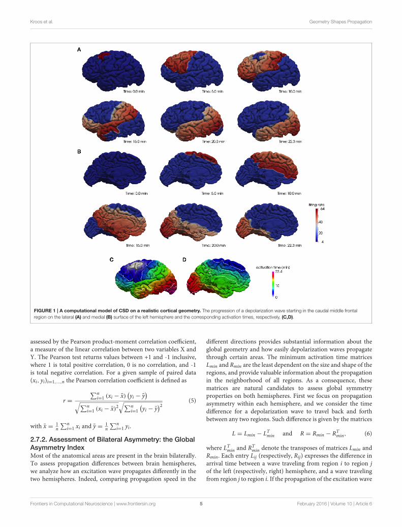
CSD is known to originate from the visual cortex, but to gaindeeper insight in the way the geometry shapes the propagation,we simulate, in both hemispheres, the spread of excitation wavesbetween all the regions of the anatomical classification. In eachsimulation, we consider as initial condition one fully depolarizedregion out of the 34 in the anatomical subdivision. Namely,we set u(0, x) = up for all x in the initially excited region,u(0, x) = u0 for all the remaining grid points and an initialuniform resting condition for the gating variable, w(0, x) = 0.Each simulation is run until all remaining regions have been fullyactivated. The arrival times of the depolarization wave in theremaining 33 regions are recorded. The only compartment thatis not considered as initially activated is the corpus callosum asit constitutes the intersection between the two hemispheres andobeys different rules for diffusion. In particular, high anisotropyvalues of white-matter tracts, as revealed by tensor diffusionimaging, yield a much larger diffusion within corpus callosumwith respect to other cortical areas. Our modeling strategy isindirectly accounting for this aspect: the mesh geometry withinthis region ismuch flatter in comparison with the other areas and,as a consequence, the simulated CSD propagation is faster.

As an illustration, we show in Figure 1 the progression ofthe depolarization wave starting from the caudal middle frontalregion and spreading across the whole cortex for the lateral (A)andmedial (B) surface of the left hemisphere. In Figures 1C,Dweplot the corresponding activation times of the whole hemisphere.

2.7. Quantities of InterestUsing the data obtained from the 34 numerical simulations perhemisphere, each one starting in a different Brodmann area, wecan introduce different ways to assess symmetry and asymmetryin the propagation, with the aim of identifying regions featuringa peculiar propagation behavior.

In any simulation, one region is initially activated, and werecord two values for each of the 33 remaining regions: theminimum and the maximum activation times. The minimumactivation time is the moment when the first point of the regionat hand gets excited, while the maximum activation time is themoment at which the last point of the region gets excited. Theminimum activation time for a given arrival region does notdepend on its shape or size, but only on the initially activatedregion and the portion of the cortex traveled by the wave betweenthe two areas. On the other hand, the maximum activation timeis also related to the shape and area of the arrival region. Thetwo recorded quantities allow to assess different aspects of thepropagation. The minimum activation time for a region providesinformation about the propagation behavior of its neighborhood.The maximum activation time is also accounting for the effect ofthe region’s geometry on the propagation.

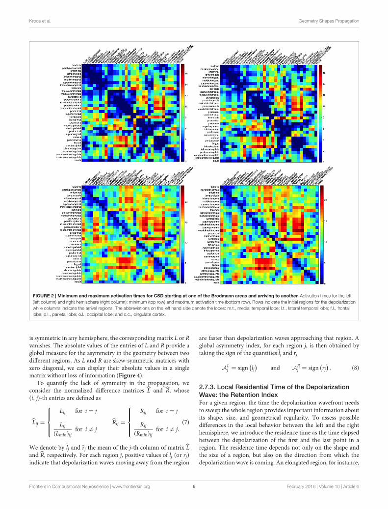
These quantities are collected into four 34 × 34 matrices,that we denote by Lmin, Lmax, Rmin, and Rmax, where L and Rrefer to the left and right hemisphere, respectively. In all of theabove matrices, rows represent the starting region of the wavepropagation, while columns the arrival region: as an example, the(i, j)-th element of Lmin represents the arrival time in region j ofa wave originated in region i.

The ordering of the regions in building such matrices playsa crucial role in the clustering of the results. Different sortingchoices, like the clustering of all regions with respect to theircentroids distances or the clustering with respect to the activationtimes, lead to different types of clustering. To emphasize thespatial connection between the regions, we chose to rearrangetheir ordering according to their affiliation to lobes. Regionsbelonging to one lobe are then clustered according to the mutualdistance of their centroids in the Euclidean norm. The minimumand maximum activation times for the left as well as for the righthemisphere are given in Figure 2.

Whatever the ordering of the regions, a lack of symmetryin the matrices Lmin and Rmin is a first clear indicator that thegeometry plays a role in shaping the propagation: if the cortexhad been spherical, an isotropic conductivity coefficient wouldhave resulted in both matrices being symmetric.

2.7.1. Correlation between Activation Times and

DistancesDespite the complex geometry of the cortex, a direct relationbetween the propagation time of wavefronts and the distancetraveled is expected. However, to further assess differencesbetween the left and right hemisphere, we explicitly relateactivation times with distances from the initially activated region.We consider the Euclidean distance between the centroids of tworegions as a proxy of the distance traveled by the wavefront.

The correlation between the distance of the centroids ofthe different regions and the different activation times can be






FIGURE 1 | A computational model of CSD on a realistic cortical geometry. The progression of a depolarization wave starting in the caudal middle frontal

region on the lateral (A) and medial (B) surface of the left hemisphere and the corresponding activation times, respectively, (C,D).

assessed by the Pearson product-moment correlation coefficient,a measure of the linear correlation between two variables X andY. The Pearson test returns values between +1 and -1 inclusive,where 1 is total positive correlation, 0 is no correlation, and -1is total negative correlation. For a given sample of paired data(xi, yi)i=1,...,n the Pearson correlation coefficient is defined as

r =

∑ni=1 (xi − x)

(yi − y

)√∑n

i=1 (xi − x)2√∑n

i=1

(yi − y

)2 (5)

with x = 1n

∑ni=1 xi and y = 1

n

∑ni=1 yi.

2.7.2. Assessment of Bilateral Asymmetry: the Global

Asymmetry IndexMost of the anatomical areas are present in the brain bilaterally.To assess propagation differences between brain hemispheres,we analyze how an excitation wave propagates differently in thetwo hemispheres. Indeed, comparing propagation speed in the

different directions provides substantial information about theglobal geometry and how easily depolarization waves propagatethrough certain areas. The minimum activation time matricesLmin and Rmin are the least dependent on the size and shape of theregions, and provide valuable information about the propagationin the neighborhood of all regions. As a consequence, thesematrices are natural candidates to assess global symmetryproperties on both hemispheres. First we focus on propagationasymmetry within each hemisphere, and we consider the timedifference for a depolarization wave to travel back and forthbetween any two regions. Such difference is given by the matrices

L = Lmin − LTmin and R = Rmin − RTmin, (6)

where LTmin and RTmin denote the transposes of matrices Lmin andRmin. Each entry Lij (respectively, Rij) expresses the difference inarrival time between a wave traveling from region i to region jof the left (respectively, right) hemisphere, and a wave travelingfrom region j to region i. If the propagation of the excitation wave






FIGURE 2 | Minimum and maximum activation times for CSD starting at one of the Brodmann areas and arriving to another. Activation times for the left

(left column) and right hemisphere (right column): minimum (top row) and maximum activation time (bottom row). Rows indicate the initial regions for the depolarization

while columns indicate the arrival regions. The abbreviations on the left hand side denote the lobes: m.t., medial temporal lobe; l.t., lateral temporal lobe; f.l., frontal

lobe; p.l., parietal lobe; o.l., occipital lobe; and c.c., cingulate cortex.

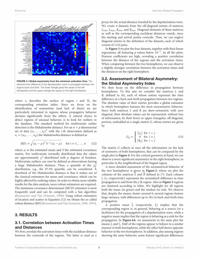
is symmetric in any hemisphere, the corresponding matrix L or Rvanishes. The absolute values of the entries of L and R provide aglobal measure for the asymmetry in the geometry between twodifferent regions. As L and R are skew-symmetric matrices withzero diagonal, we can display their absolute values in a singlematrix without loss of information (Figure 4).

To quantify the lack of symmetry in the propagation, weconsider the normalized difference matrices L and R, whose(i, j)-th entries are defined as

Lij =

Lij for i = j

Lij

(Lmin)ijfor i 6= j

Rij =

Rij for i = j

Rij

(Rmin)ijfor i 6= j.

(7)

We denote by lj and rj the mean of the j-th column of matrix Land R, respectively. For each region j, positive values of lj (or rj)indicate that depolarization waves moving away from the region

are faster than depolarization waves approaching that region. Aglobal asymmetry index, for each region j, is then obtained bytaking the sign of the quantities lj and rj

ALj = sign

(lj)

and ARj = sign

(rj). (8)

2.7.3. Local Residential Time of the Depolarization

Wave: the Retention IndexFor a given region, the time the depolarization wavefront needsto sweep the whole region provides important information aboutits shape, size, and geometrical regularity. To assess possibledifferences in the local behavior between the left and the righthemisphere, we introduce the residence time as the time elapsedbetween the depolarization of the first and the last point in aregion. The residence time depends not only on the shape andthe size of a region, but also on the direction from which thedepolarization wave is coming. An elongated region, for instance,






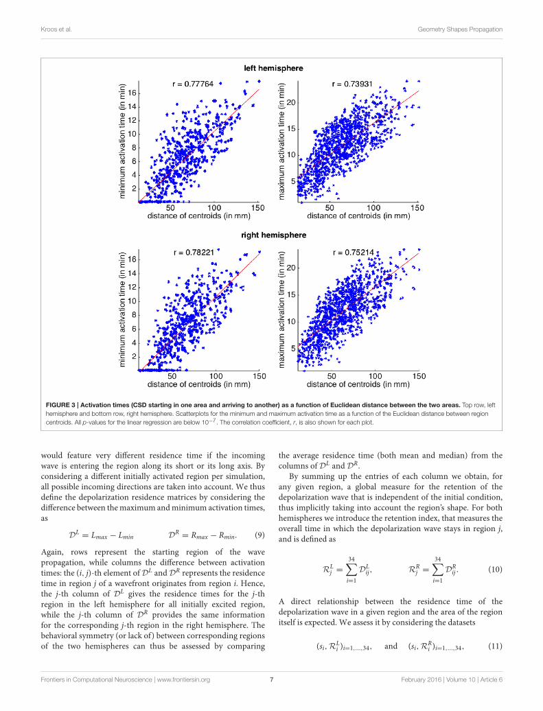
FIGURE 3 | Activation times (CSD starting in one area and arriving to another) as a function of Euclidean distance between the two areas. Top row, left

hemisphere and bottom row, right hemisphere. Scatterplots for the minimum and maximum activation time as a function of the Euclidean distance between region

centroids. All p-values for the linear regression are below 10−7. The correlation coefficient, r, is also shown for each plot.

would feature very different residence time if the incomingwave is entering the region along its short or its long axis. Byconsidering a different initially activated region per simulation,all possible incoming directions are taken into account. We thusdefine the depolarization residence matrices by considering thedifference between themaximum andminimum activation times,as

DL = Lmax − Lmin D

R = Rmax − Rmin. (9)

Again, rows represent the starting region of the wavepropagation, while columns the difference between activationtimes: the (i, j)-th element ofDL andDR represents the residencetime in region j of a wavefront originates from region i. Hence,the j-th column of DL gives the residence times for the j-thregion in the left hemisphere for all initially excited region,while the j-th column of DR provides the same informationfor the corresponding j-th region in the right hemisphere. Thebehavioral symmetry (or lack of) between corresponding regionsof the two hemispheres can thus be assessed by comparing

the average residence time (both mean and median) from thecolumns of DL and DR.

By summing up the entries of each column we obtain, forany given region, a global measure for the retention of thedepolarization wave that is independent of the initial condition,thus implicitly taking into account the region’s shape. For bothhemispheres we introduce the retention index, that measures theoverall time in which the depolarization wave stays in region j,and is defined as

RLj =

34∑

i=1

DLij, R

Rj =

34∑

i=1

DRij . (10)

A direct relationship between the residence time of thedepolarization wave in a given region and the area of the regionitself is expected. We assess it by considering the datasets

(si,RLi )i=1,...,34, and (si,R

Ri )i=1,...,34, (11)






FIGURE 4 | Global asymmetry from the minimum activation time. The

absolute time difference of the depolarization wave to propagate between two

regions back and forth. The lower triangle gives the values of the left

hemisphere and the upper triangle the values for the right hemisphere.

where si describes the surface of region i and Ri thecorresponding retention index. Since we focus on theidentification of symmetries (and lack of them) we areparticularly interested in regions whose propagative behaviordeviates significantly from the others. A natural choice todetect regions of unusual behavior, is to look for outliers inthe database. The standard method for multivariate outlierdetection is the Mahalonobis distance. For an n× p dimensionalset of data (x1, . . . , xn)

T with the i-th observation defined asxi = (xi1, . . . , xip) the Mahalonobis distance is defined as

MDi =

√(xi − µ)T S−1 (xi − µ) for i = 1, . . . , n (12)

where µ is the estimated mean and S the estimated covariancematrix. For multivariate normally distributed data the valuesare approximately χ2-distributed with p degrees of freedom.Multivariate outliers can now be defined as observations havinga large Mahalonobis distance. Thus, a quantile of the χ2

p

distribution, e.g., the 97.5% quantile, can be considered. Adrawback of the Mahalonobis distance is that it makes use ofthe classical estimators for mean and covariance, which can behighly affected by outlying values. In order to obtainmore reliableresults for the data analysis, more robust estimators are required.The minimum covariance determinant (MCD) estimator is mostfrequently used and can be computed with a fast algorithm(Rousseeuw and Van Driessen, 1999). Using robust estimatorsof location and scatter in Equation (12) we obtain the so calledrobust distance (RD) (Rousseeuw and Van Zomeren, 1990, 1991).

.

3. RESULTS

3.1. Correlation between Activation Timesand DistancesWe first correlate the activation times with the euclidean distancebetween the centroids of the regions. The latter is used as a

proxy for the actual distance traveled by the depolarization wave.We create 4 datasets from the off-diagonal entries of matricesLmin, Lmax, Rmin, and Rmax. Diagonal elements of these matricesas well as the corresponding euclidean distances vanish, sincethe starting and arrival points coincide. Thus, we can neglectdiagonal entries in the definition of the datasets, each of whichconsist of 1122 pairs.

In Figure 3we plot the four datasets, together with their linearregressions, all featuring p-values below 10−7. In all the plots,Pearson coefficients are high, revealing a positive correlationbetween the distance of the regions and the activation times.When comparing between the two hemispheres, we can observea slightly stronger correlation between the activation times andthe distances on the right hemisphere.

3.2. Assessment of Bilateral Asymmetry:the Global Asymmetry IndexWe then focus on the difference in propagation betweenhemispheres. To this aim we consider the matrices L andR, defined in (6), each of whose entries represent the timedifference in a back-and-forth propagation between two regions.The absolute value of their entries provides a global estimatorto which hemisphere features the most unsymmetric behavior.Since both matrices L and R are skew-symmetric with zerodiagonal, their absolute values can be represented, without lossof information, by their lower or upper triangular, off-diagonal,portion, embedded in a single matrix G, whose entries are givenby

Gij =

∣∣Lij∣∣ for i > j

0 for i = j∣∣Rij∣∣ for i < j

(13)

The matrix G collects at once all the information on the lackof symmetry of both hemispheres, that can be compared by thesingle plot in Figure 4. For the cortical geometry at hand, we canobserve a more significant asymmetry in the right hemisphere, inparticular in the neighborhood of the lingual region.

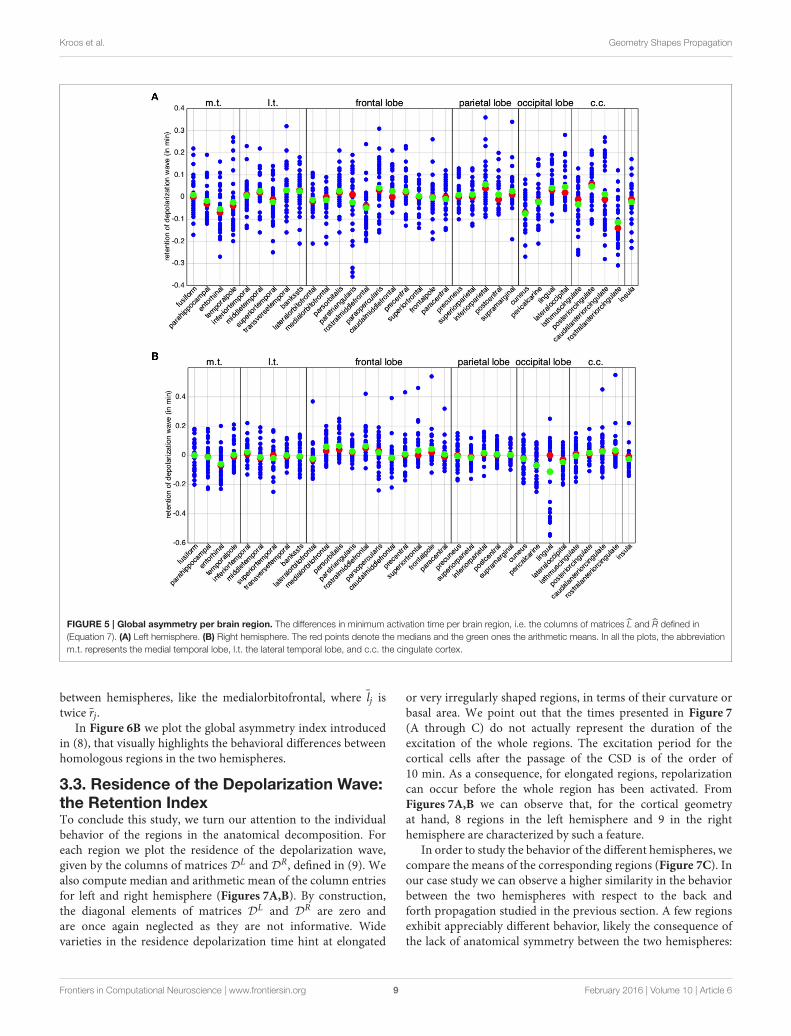
A more detailed assessment of the asymmetrical behavior ofthe two hemispheres is given in Figure 5, where we plot thecolumns of the matrices L and R defined in (7). Each columnlj (rj, respectively) represents the normalized difference in timepropagation to and from the j-th region. Also in Figure 5 regionsare clustered according to lobes. We highlight for all regionsboth the mean (in green) and the median (in red). We observethat, despite the means cluster around 0, several regions featurelarge variance, with differences up to 36 s in back-and-forth timepropagation.

A positive mean lj (respectively, rj) implies that thecorresponding region is, in general, behaving as a source (or afacilitator) for the propagation of a depolarization wave, while anegative mean implies that the region is behaving as a sink for thepropagation. In Figure 6A, we summarize in the same plot themeans lj and rj. Half of the regions appear to behave in a similarmanner in both hemispheres, while the other half shows oppositebehavior in the two hemispheres. In addition, also among regionsshowing the same behavior, some feature significant differences






FIGURE 5 | Global asymmetry per brain region. The differences in minimum activation time per brain region, i.e. the columns of matrices L and R defined in

(Equation 7). (A) Left hemisphere. (B) Right hemisphere. The red points denote the medians and the green ones the arithmetic means. In all the plots, the abbreviation

m.t. represents the medial temporal lobe, l.t. the lateral temporal lobe, and c.c. the cingulate cortex.

between hemispheres, like the medialorbitofrontal, where lj istwice rj.

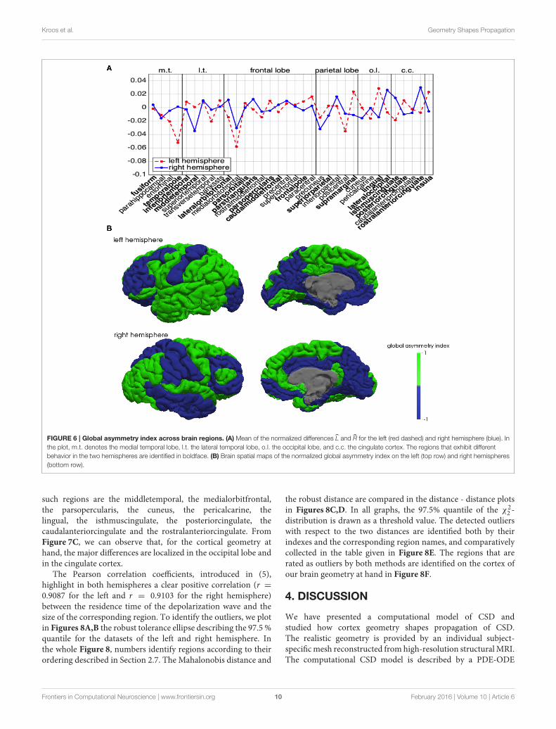
In Figure 6B we plot the global asymmetry index introducedin (8), that visually highlights the behavioral differences betweenhomologous regions in the two hemispheres.

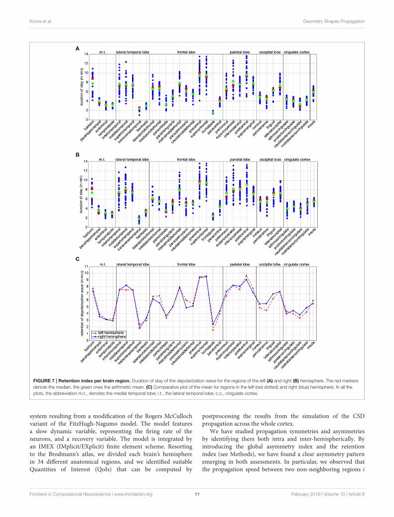
3.3. Residence of the Depolarization Wave:the Retention IndexTo conclude this study, we turn our attention to the individualbehavior of the regions in the anatomical decomposition. Foreach region we plot the residence of the depolarization wave,given by the columns of matrices DL and DR, defined in (9). Wealso compute median and arithmetic mean of the column entriesfor left and right hemisphere (Figures 7A,B). By construction,the diagonal elements of matrices DL and DR are zero andare once again neglected as they are not informative. Widevarieties in the residence depolarization time hint at elongated

or very irregularly shaped regions, in terms of their curvature orbasal area. We point out that the times presented in Figure 7

(A through C) do not actually represent the duration of theexcitation of the whole regions. The excitation period for thecortical cells after the passage of the CSD is of the order of10 min. As a consequence, for elongated regions, repolarizationcan occur before the whole region has been activated. FromFigures 7A,B we can observe that, for the cortical geometryat hand, 8 regions in the left hemisphere and 9 in the righthemisphere are characterized by such a feature.

In order to study the behavior of the different hemispheres, wecompare the means of the corresponding regions (Figure 7C). Inour case study we can observe a higher similarity in the behaviorbetween the two hemispheres with respect to the back andforth propagation studied in the previous section. A few regionsexhibit appreciably different behavior, likely the consequence ofthe lack of anatomical symmetry between the two hemispheres:






FIGURE 6 | Global asymmetry index across brain regions. (A) Mean of the normalized differences L and R for the left (red dashed) and right hemisphere (blue). In

the plot, m.t. denotes the medial temporal lobe, l.t. the lateral temporal lobe, o.l. the occipital lobe, and c.c. the cingulate cortex. The regions that exhibit different

behavior in the two hemispheres are identified in boldface. (B) Brain spatial maps of the normalized global asymmetry index on the left (top row) and right hemispheres

(bottom row).

such regions are the middletemporal, the medialorbitfrontal,the parsopercularis, the cuneus, the pericalcarine, thelingual, the isthmuscingulate, the posteriorcingulate, thecaudalanteriorcingulate and the rostralanteriorcingulate. FromFigure 7C, we can observe that, for the cortical geometry athand, the major differences are localized in the occipital lobe andin the cingulate cortex.

The Pearson correlation coefficients, introduced in (5),highlight in both hemispheres a clear positive correlation (r =

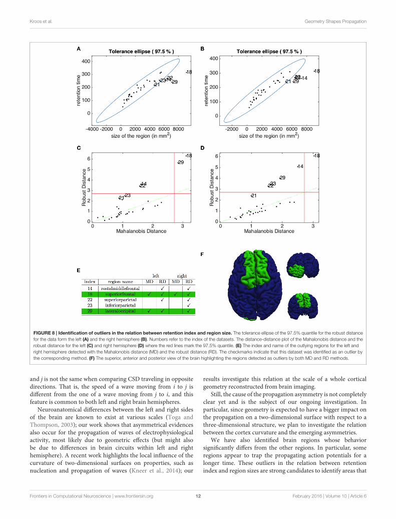
0.9087 for the left and r = 0.9103 for the right hemisphere)between the residence time of the depolarization wave and thesize of the corresponding region. To identify the outliers, we plotin Figures 8A,B the robust tolerance ellipse describing the 97.5 %quantile for the datasets of the left and right hemisphere. Inthe whole Figure 8, numbers identify regions according to theirordering described in Section 2.7. The Mahalonobis distance and

the robust distance are compared in the distance - distance plotsin Figures 8C,D. In all graphs, the 97.5% quantile of the χ2

2 -distribution is drawn as a threshold value. The detected outlierswith respect to the two distances are identified both by theirindexes and the corresponding region names, and comparativelycollected in the table given in Figure 8E. The regions that arerated as outliers by both methods are identified on the cortex ofour brain geometry at hand in Figure 8F.

4. DISCUSSION

We have presented a computational model of CSD andstudied how cortex geometry shapes propagation of CSD.The realistic geometry is provided by an individual subject-specificmesh reconstructed from high-resolution structuralMRI.The computational CSD model is described by a PDE-ODE






FIGURE 7 | Retention index per brain region. Duration of stay of the depolarization wave for the regions of the left (A) and right (B) hemisphere. The red markers

denote the median, the green ones the arithmetic mean. (C) Comparative plot of the mean for regions in the left (red dotted) and right (blue) hemisphere. In all the

plots, the abbreviation m.t., denotes the medial temporal lobe; l.t., the lateral temporal lobe; c.c., cingulate cortex.

system resulting from a modification of the Rogers McCullochvariant of the FitzHugh-Nagumo model. The model featuresa slow dynamic variable, representing the firing rate of theneurons, and a recovery variable. The model is integrated byan IMEX (IMplicit/EXplicit) finite element scheme. Resortingto the Brodmann’s atlas, we divided each brain’s hemispherein 34 different anatomical regions, and we identified suitableQuantities of Interest (QoIs) that can be computed by

postprocessing the results from the simulation of the CSDpropagation across the whole cortex.

We have studied propagation symmetries and asymmetriesby identifying them both intra and inter-hemispherically. Byintroducing the global asymmetry index and the retentionindex (see Methods), we have found a clear asymmetry patternemerging in both assessments. In particular, we observed thatthe propagation speed between two non-neighboring regions i






FIGURE 8 | Identification of outliers in the relation between retention index and region size. The tolerance ellipse of the 97.5% quantile for the robust distance

for the data form the left (A) and the right hemisphere (B). Numbers refer to the index of the datasets. The distance-distance plot of the Mahalonobis distance and the

robust distance for the left (C) and right hemisphere (D) where the red lines mark the 97.5% quantile. (E) The index and name of the outlying regions for the left and

right hemisphere detected with the Mahalonobis distance (MD) and the robust distance (RD). The checkmarks indicate that this dataset was identified as an outlier by

the corresponding method. (F) The superior, anterior and posterior view of the brain highlighting the regions detected as outliers by both MD and RD methods.

and j is not the same when comparing CSD traveling in oppositedirections. That is, the speed of a wave moving from i to j isdifferent from the one of a wave moving from j to i, and thisfeature is common to both left and right brain hemispheres.

Neuroanatomical differences between the left and right sidesof the brain are known to exist at various scales (Toga andThompson, 2003); our work shows that asymmetrical evidencesalso occur for the propagation of waves of electrophysiologicalactivity, most likely due to geometric effects (but might alsobe due to differences in brain circuits within left and righthemisphere). A recent work highlights the local influence of thecurvature of two-dimensional surfaces on properties, such asnucleation and propagation of waves (Kneer et al., 2014); our

results investigate this relation at the scale of a whole corticalgeometry reconstructed from brain imaging.

Still, the cause of the propagation asymmetry is not completelyclear yet and is the subject of our ongoing investigation. Inparticular, since geometry is expected to have a bigger impact onthe propagation on a two-dimensional surface with respect to athree-dimensional structure, we plan to investigate the relationbetween the cortex curvature and the emerging asymmetries.

We have also identified brain regions whose behaviorsignificantly differs from the other regions. In particular, someregions appear to trap the propagating action potentials for alonger time. These outliers in the relation between retentionindex and region sizes are strong candidates to identify areas that






may play a key role in the CSD propagation (and possibly beable to stop it). Such information would be relevant to designtherapies using stereotactic cortical neuromodulation, wheretarget structures for modulation have to be carefully selected,see, e.g., Dahlem et al. (2015). Implementing an individualizedcomputational model for CSD would improve the clinicaleffectiveness of these therapies.

In this paper we have modeled the diffusion tensor asisotropic, with all eigenvalues being equal to a constant δ.However, diffusion tensor imaging (DTI) provides, per a givenvoxel in the image, a more realistic (strongly anisotropic) tensorfor the diffusion of water molecules across white-matter tracts.We expect that more personalized conductivity values, takinginto account information from DTI data, can provide a betterinsight on the regions that are principally responsible for this lackof symmetrical behavior.

The model can benefit from the incorporation of otheringredients. An important limitation of our study is that thediffusion model does not account for long-range connections.Rather than adopting one of the many computational strategiesto model such features within a circuit (for instance, byadding random edges between far-separated mesh nodes), wepreferred to just focus on short-range connections associatedto excitatory connectivity. In addition, we have not modeledcortical inhibition, which is a well-known mechanism forcontrolling propagation of neuronal excitability in corticalcircuits. Incorporating inhibitory neurons and long-rangeconnections within the diffusion model will be of specialinterest for future research on CSD modeling. Indeed, long-range inhibitory connections have been found in several sensorycortices where they play a key role in stabilizing strong increasesof electrical activity. Notice that, the presence of inhibition, inaddition to make the model more realistic, will scale the diffusionconstants, making them several orders of magnitude higher inorder to produce CSD propagating at the macroscale with atime duration of about 20 min. Moreover, the incorporation ofshort-time synaptic plasticity, including synaptic depression andfacilitation (Markram and Tsodyks, 1996; Tsodyks and Markram,1997) makes neural connectivity to be activity-dependent, addingnew non-linearities into the model which might strongly affectthe stability of CSD propagation (Cortes et al., 2013). Finally,the use of a more detailed neuronal model, instead of the firingrate slow dynamics at the basis of our analysis, would allow to

study, at the cost of increased computational effort, the impactof channelopathies in favoring or countering the propagationof CSD.

To conclude, some words have to be said in relation to thedisease. Based on the evidence that CSD has been proposedto be a neural correlate of aura migraine, we have presented amethod that addresses dynamical features of CSD propagatingon a realistic (subject-specific) cortical geometry. Computationalmodels of migraine, in synergy with the analysis of alteredprocessing of sensory stimuli (de Tommaso et al., 2014), notonly provide further insight in this disease, but they are alsofundamental in constructing new interventional approaches. Thecortical data we used in this paper is coming from an healthybrain, and can provide a baseline for the QoIs that we identified.

Whether the results shown here remain valid or not, andasymmetries are enhanced when simulations are run on a meshcoming from a patient suffering from aura migraine, is for usan obligated matter for future research. The occurrence of largerdeviations from the baseline in unhealthy people, would makethe QoIs introduced in this paper able to discriminate healthyfrom unhealthy patients, and, at the same time, able to identifysubjects potentially susceptible of suffering from migraine aura.We expect further insight in this direction by the extensiveapplication of our analysis to a statistically significant sample ofpatients.

ACKNOWLEDGMENTS

This research is supported by Bizkaia Talent and EuropeanCommission through COFUND under the grant BRAhMS– Brain Aura Mathematical Simulation – (AYD-000-285),and also by the Basque Government through the BERC2014–2017 program and by Spanish Ministry of Economy andCompetitiveness MINECO: BCAM Severo Ochoa excellenceaccreditation SEV-2013-0323. JMC acknowledges financialsupport from Ikerbasque: The Basque Foundation for Scienceand Euskampus at UPV/EHU.

SUPPLEMENTARY MATERIAL

The Supplementary Material for this article can be foundonline at: http://journal.frontiersin.org/article/10.3389/fncom.2016.00006

REFERENCES

Brodmann, K. (2006). Brodmann’s Localisation in the Cerebral Cortex - The

Principles of Comparative Localisation in the Cerebral Cortex Based on

Cytoarchitectonics. New York, NY: Springer US.

Cortes, J. M., Desroches, M., Rodrigues, S., Veltze, R., Muñoz, M., and Sejnowski,

T. J. (2013). Short-term synaptic plasticity in the deterministic Tsodyks-

Markram model leads to unpredictable network dynamics. Proc. Natl. Acad.

Sci. U.S.A. 110, 16610–16615. doi: 10.1073/pnas.1316071110

Cortes, J. M., Marinazzo, D., Series, P., Oram, M. W., Sejnowski, T. J., and

van Rossum, M. C. (2012). The effect of neural adaptation on population

coding accuracy. J. Comput. Neurosci. 32, 387–402. doi: 10.1007/s10827-011-

0358-4

Cressman, J., Ullah, G., Ziburkus, J., Schiff, S., and Barreto, E. (2009). The influence

of sodium and potassium dynamics on excitability, seizure, and the stability of

persistent states: I. single neuron dynamics. J. Comput. Neurosci. 26, 159–170.

doi: 10.1007/s10827-008-0132-4

Dahlem, M. A., Schmidt, B., Bojak, I., Boie, S., Kneer, F., Hadjikhani, N., et al.

(2015). Cortical hot spots and labyrinths: why cortical neuromodulation for

episodic migraine with aura should be personalized. Front. Comput. Neurosci.

9:29. doi: 10.3389/fncom.2015.00029

de Tommaso, M., Ambrosini, A., Brighina, B., Coppola, G., Perrotta, A., Pierelli,

F., et al. (2014). Altered processing of sensory stimuli in patients with migraine.

Nat. Rev. Neurol. 10, 144–155. doi: 10.1038/nrneurol.2014.14

Diez, I., Bonifazi, P., Escudero, I., Mateos, B., Muñoz, M. A., Stramaglia,

S., et al. (2015). A novel brain partition highlights the modular skeleton


http://journal.frontiersin.org/article/10.3389/fncom.2016.00006





shared by structure and function. Sci. Rep. 5, 10532. doi: 10.1038/srep

10532

Fischl, B. (2012). Freesurfer. Neuroimage 62, 774–781. doi: 10.1016/j.neuroimage.

2012.01.021

Fitzhugh, R. (1961). Impulses and physiological states in theoretical models

of nerve membrane. Biophys. J. 1, 445–466. doi: 10.1016/S0006-3495(61)

86902-6

Hadjikhani, N., Sanchez Del Rio, M., Wu, O., Schwartz, D., Bakker, D., Fischl,

B., et al. (2001). Mechnisms of migraine aura revealed by functional mri

in human visual cortex. Proc. Natl. Acad. Sci. U.S.A. 98, 4687–4692. doi:

10.1073/pnas.071582498

Izhikevich, E. (2007). Dynamical Systems in Neuroscience: The Geometry of

Excitability and Bursting (Computational Neuroscience). Cambridge, MA: MIT

Press.

Kandel, E., Schwartz, J., and Jessell, T. (2000). Principles of Neural Science. New

York, NY: McGraw-Hill.

Kneer, F., Schöll, E., and Dahlem, M. A. (2014). Nucleation of reaction-

diffusion waves on curved surfaces. New J. Phys. 16:053010. doi: 10.1088/1367-

2630/16/5/053010

Kraio, R. P., and Nicholson, C. (1978). Extracellular ionic variations

during spreading depression. Neuroscience 3, 1045–1059. doi:

10.1016/0306-4522(78)90122-7

Leão, A. (1944). Spreading depression of activity in the cerebral cortex. J.

Neurophysiol. 7, 391–396.

Leão, A. (1947). Further observations on the spreading depression of activity in the

cerebral cortex. J. Neurophysiol. 10, 409–414.

Markram, H., and Tsodyks, M. (1996). Redistribution of synaptic efficacy between

neocortical pyramidal neurons. Nature 382, 807–810. doi: 10.1038/382807a0

Pocci, C., Moussa, A., Hubert, F., and Chapuisat, G. (2010). Numerical study

of the stopping of aura during migraine. Proc. ESAIM 30, 4–52. doi:

10.1051/proc/2010005

Porooshani, H., Porooshani, A., Gannon, L., and Kyle, G. (2004). Speed of

progression of migrainous visual aura measured by sequential field assessment.

Neuro Ophthalmol. 28, 101–105. doi: 10.1076/noph.28.2.101.23739

Quarteroni, A., and Valli, A. (1997). Numerical Approximation of Partial

Differential Equations, 2nd Edn. Berlin; Heidelberg: Springer-Verlag.

Reggia, J. A., and Montgomery, D. (1996). A computational model of visual

hallucinations in migraine. Comput. Biol. Med. 26, 133–141. doi: 10.1016/0010-

4825(95)00051-8

Richter, F., and Lehmenkühler, A. (2008). Cortical spreading depression (csd): a

neurophysiological correlate of migraine aura. Der Schmerz 22, 544–550. doi:

10.1007/s00482-008-0653-9

Rogers, J. M., and McCulloch, A. D. (1994). A collocation - galerkin finite element

model of cardiac action potential propagation. IEEE Trans Biomed Eng. 41,

743–757. doi: 10.1109/10.310090

Rousseeuw, P., and Van Driessen, K. (1999). A fast algorithm for the

minimum covariance determinant estimator. Technometrics 41, 212–223. doi:

10.1080/00401706.1999.10485670

Rousseeuw, P., and Van Zomeren, B. (1990). Unmasking multivariant

outliers and leverage points. J. Am. Stat. Assoc. 85, 633–639. doi:

10.1080/01621459.1990.10474920

Rousseeuw, P., and Van Zomeren, B. (1991). Robust Distances: Simulations and

Cutoff Values, Vol. 34. New York, NY: Springer-Verlag.

Saad, Y. (2003). Iterative Methods for Sparse Linear Systems, 2nd Edn. Philadelphia,

PA: Society for Industrial and Applied Mathematics.

Sanides, F. (1962). “Die architektonik des menschlichen stirnhirns,” in

Monographien aus dem Gesamtegebiete der Neurologie und Psychiatrie,

Vol. 98. eds M. Müller, H. Spatz, and P. Vogel (Berlin: Springer). doi:

10.1007/978-3-642-86210-6

Ségonne, F., Dale, A. M., Busa, E., Glessner, M., Salat, D., Hahn, H. K., et al. (2004).

A hybrid approach to the skull stripping problem in MRI. Neuroimage 22,

1060–1075. doi: 10.1016/j.neuroimage.2004.03.032

Toga, A. W., and Thompson, P. M. (2003). Mapping brain asymmetry. Nat. Rev.

Neurosci. 4, 37–48. doi: 10.1038/nrn1009

Tsodyks, M. V., and Markram, H. (1997). The neural code between neocortical

pyramidal neurons depends on neurotransmitter release probability. Proc. Natl.

Acad. Sci. U.S.A. 94, 719–723. doi: 10.1073/pnas.94.2.719

Tuckwell, H. C., and Miura, R. M. (1978). A mathematical model for spreading

cortical depression. Biophys. J. 23, 257–276. doi: 10.1016/S0006-3495(78)

85447-2

Vos, T., Flaxman, A. D., Naghavi, M., Lozano, R., Michaud, C., Ezzati, M., et al.

(2012). Years lived with disability (ylds) for 1160 sequelae of 289 diseases and

injuries 1990-2010: a systematic analysis for the global burden of disease study

2010. Lancet 380, 2163–2196. doi: 10.1016/S0140-6736(12)61729-2

Conflict of Interest Statement: The authors declare that the research was

conducted in the absence of any commercial or financial relationships that could

be construed as a potential conflict of interest.

The reviewer Dr Wang and handling Editor, Dr Wu declared their shared

affiliation, and the handling Editor states that the process nevertheless met the

standards of a fair and objective review.

Copyright © 2016 Kroos, Diez, Cortes, Stramaglia and Gerardo-Giorda. This is an

open-access article distributed under the terms of the Creative Commons Attribution

License (CC BY). The use, distribution or reproduction in other forums is permitted,

provided the original author(s) or licensor are credited and that the original

publication in this journal is cited, in accordance with accepted academic practice.

No use, distribution or reproduction is permitted which does not comply with these

terms.


http://creativecommons.org/licenses/by/4.0/








Documents

Geometry Shapes Propagation: Assessing the Presence and … · 2017-04-13 · Kroos et al. Geometry Shapes Propagation (de Tommaso et al., 2014). Starting in the visual cortex, CSD