Embed Size (px)
Citation preview

HAL Id: hal-00870603https://hal.archives-ouvertes.fr/hal-00870603
Preprint submitted on 7 Oct 2013
HAL is a multi-disciplinary open accessarchive for the deposit and dissemination of sci-entific research documents, whether they are pub-lished or not. The documents may come fromteaching and research institutions in France orabroad, or from public or private research centers.
L’archive ouverte pluridisciplinaire HAL, estdestinée au dépôt et à la diffusion de documentsscientifiques de niveau recherche, publiés ou non,émanant des établissements d’enseignement et derecherche français ou étrangers, des laboratoirespublics ou privés.
Shapes of polyhedra, mixed volumes, and hyperbolicgeometry
François Fillastre, Ivan Izmestiev
To cite this version:François Fillastre, Ivan Izmestiev. Shapes of polyhedra, mixed volumes, and hyperbolic geometry.2013. hal-00870603

SHAPES OF POLYHEDRA, MIXED VOLUMES, AND
HYPERBOLIC GEOMETRY
FRANCOIS FILLASTRE AND IVAN IZMESTIEV
Abstract. We are generalizing to higher dimensions the Bavard-Ghysconstruction of the hyperbolic metric on the space of polygons with fixeddirections of edges.
The space of convex d-dimensional polyhedra with fixed directionsof facet normals has a decomposition into type cones that correspondto different combinatorial types of polyhedra. This decomposition is asubfan of the secondary fan of a vector configuration and can be analyzedwith the help of Gale diagrams.
We construct a family of quadratic forms on each of the type conesusing the theory of mixed volumes. The Alexandrov-Fenchel inequalitiesensure that these forms have exactly one positive eigenvalue. This intro-duces a piecewise hyperbolic structure on the space of similarity classesof polyhedra with fixed directions of facet normals. We show that someof the dihedral angles on the boundary of the resulting cone-manifoldare equal to π
2.
Contents
Introduction 2Motivation 2Outline of the paper 2Related work 3Acknowledgements 31. Shapes of polyhedra 31.1. Normally equivalent polyhedra and type cones 31.2. Secondary fans 121.3. Examples 262. Mixed volumes 322.1. The examples, continued 322.2. Mixed volumes and quadratic forms 343. Hyperbolic geometry 393.1. From type cones to hyperbolic polyhedra 393.2. The examples, continued 403.3. Dihedral angles at the boundary 443.4. Cone angles in the interior 453.5. Questions 474. Related work 484.1. The first weight space and the discrete Christoffel problem 48
Date: September 30, 2013.Supported by the European Research Council under the European Union’s Seventh
Framework Programme (FP7/2007-2013)/ERC Grant agreement no. 247029-SDModels.
1
2 FRANCOIS FILLASTRE AND IVAN IZMESTIEV
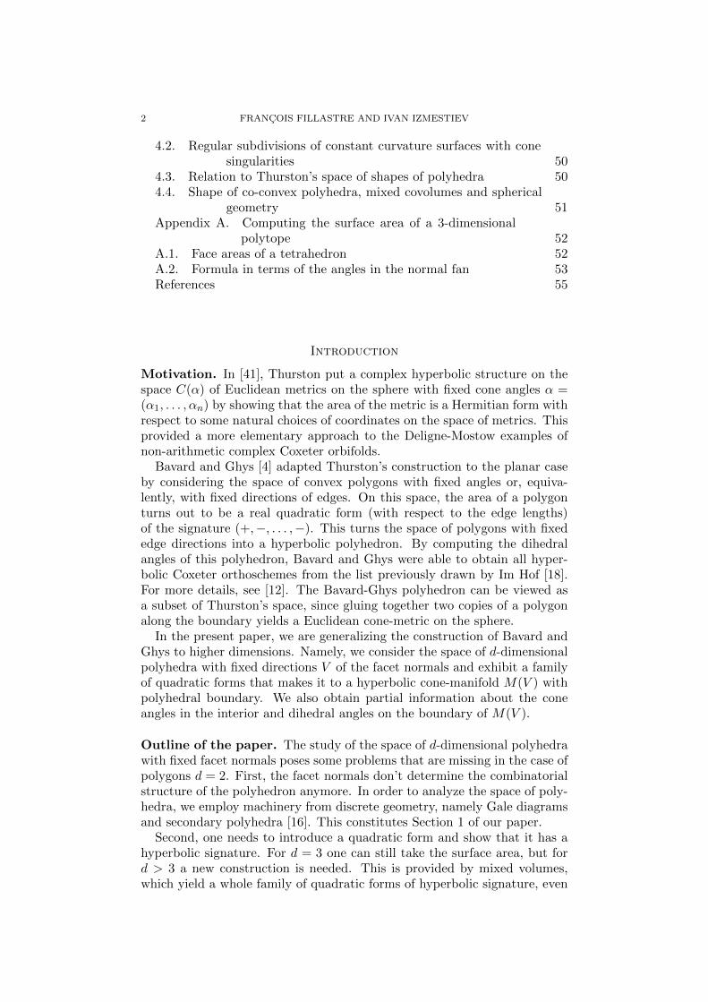
4.2. Regular subdivisions of constant curvature surfaces with conesingularities 50
4.3. Relation to Thurston’s space of shapes of polyhedra 504.4. Shape of co-convex polyhedra, mixed covolumes and spherical
geometry 51Appendix A. Computing the surface area of a 3-dimensional
polytope 52A.1. Face areas of a tetrahedron 52A.2. Formula in terms of the angles in the normal fan 53References 55
Introduction
Motivation. In [41], Thurston put a complex hyperbolic structure on thespace C(α) of Euclidean metrics on the sphere with fixed cone angles α =(α1, . . . , αn) by showing that the area of the metric is a Hermitian form withrespect to some natural choices of coordinates on the space of metrics. Thisprovided a more elementary approach to the Deligne-Mostow examples ofnon-arithmetic complex Coxeter orbifolds.
Bavard and Ghys [4] adapted Thurston’s construction to the planar caseby considering the space of convex polygons with fixed angles or, equiva-lently, with fixed directions of edges. On this space, the area of a polygonturns out to be a real quadratic form (with respect to the edge lengths)of the signature (+,−, . . . ,−). This turns the space of polygons with fixededge directions into a hyperbolic polyhedron. By computing the dihedralangles of this polyhedron, Bavard and Ghys were able to obtain all hyper-bolic Coxeter orthoschemes from the list previously drawn by Im Hof [18].For more details, see [12]. The Bavard-Ghys polyhedron can be viewed asa subset of Thurston’s space, since gluing together two copies of a polygonalong the boundary yields a Euclidean cone-metric on the sphere.
In the present paper, we are generalizing the construction of Bavard andGhys to higher dimensions. Namely, we consider the space of d-dimensionalpolyhedra with fixed directions V of the facet normals and exhibit a familyof quadratic forms that makes it to a hyperbolic cone-manifold M(V ) withpolyhedral boundary. We also obtain partial information about the coneangles in the interior and dihedral angles on the boundary of M(V ).
Outline of the paper. The study of the space of d-dimensional polyhedrawith fixed facet normals poses some problems that are missing in the case ofpolygons d = 2. First, the facet normals don’t determine the combinatorialstructure of the polyhedron anymore. In order to analyze the space of poly-hedra, we employ machinery from discrete geometry, namely Gale diagramsand secondary polyhedra [16]. This constitutes Section 1 of our paper.
Second, one needs to introduce a quadratic form and show that it has ahyperbolic signature. For d = 3 one can still take the surface area, but ford > 3 a new construction is needed. This is provided by mixed volumes,which yield a whole family of quadratic forms of hyperbolic signature, even

SHAPES OF POLYHEDRA, MIXED VOLUMES, AND HYPERBOLIC GEOMETRY 3
for d = 3. The signature of the quadratic form is ensured by the Alexandrov-Fenchel inequalities. This aspect is discussed in Section 2.
Finally, the dihedral angles are now more difficult to compute. Positiveand negative results in this direction are contained in Section 3.
Figure 1. The space of polyhedra with face normals parallelto those of a triangular bipyramid is a right-angled hyperbolichexagon.
All along the paper we are analyzing several examples. One of them isgiven by the space of 3-dimensional polyhedra with 6 faces whose normals areparallel to those of a triangular bipyramid, Figure 1 left. Translating eachface independently yields 6 different combinatorial types, and the space ofall polyhedra up to similarity forms a 2-dimensional polyhedral complex onFigure 1 middle. The surface area is a quadratic form of signature (+,−,−)on the space of polyhedra, which puts a hyperbolic metric on the complexmaking it a right-angled hyperbolic hexagon, Figure 1 right.
Related work. A different generalization (and dualization) of the Bavard-Ghys construction was given by Kapovich and Millson [22, 23] who consid-ered the space of polygonal lines in R3 with fixed edge lengths.
By Alexandrov’s theorem [2], every Euclidean metric with cone anglesαi < 2π is the intrinsic metric on the boundary of a unique convex polyhe-dron in R3. Thus Thurston’s space is the space of all convex polyhedra withfixed solid exterior angles at the vertices. A link between our constructionand that of Thurston is discussed in Section 4 that contains also a numberof other connections to discrete and hyperbolic geometry.
Acknowledgements. The authors thank Haruko Nishi, Arnau Padrol, Fran-cisco Santos, and Raman Sanyal for interesting discussions. Part of thiswork was done during the visit of the first author to FU Berlin and the visitof the second author to the university of Cergy-Pontoise. We thank bothinstitutions for hospitality.
1. Shapes of polyhedra
1.1. Normally equivalent polyhedra and type cones.
1.1.1. Convex polyhedra, polytopes, cones. A convex polyhedron P ⊂ Rdis an intersection of finitely many closed half-spaces. A bounded convexpolyhedron is called polytope; equivalently, a polytope is the convex hull offinitely many points.

4 FRANCOIS FILLASTRE AND IVAN IZMESTIEV
By aff(P ) we denote the affine hull of P , that is the smallest affine sub-space of Rd containing P . The dimension of a convex polyhedron is thedimension of its affine hull.
A hyperplane H is called a supporting hyperplane of a convex polyhedronP if H ∩ P 6= ∅ while P lies in one of the closed half-spaces boundedby H. The intersection P ∩ H is called a face of P (sometimes it makessense to consider ∅ and P as faces of P , too). Faces of dimensions 0, 1, anddimP−1 are called vertices, edges, and facets, respectively. A d-dimensionalpolytope is called simple, if each of its vertices belongs to exactly d facets(equivalently, to exactly d edges).
A convex polyhedral cone is the intersection of finitely many closed half-spaces whose boundary hyperplanes pass all through the origin. Equiva-lently, it is the positive hull
posw1, w2, . . . , wk :=
k∑i=1
λiwi | λi ≥ 0, i = 1, . . . , k
of finitely many vectors. A cone is called pointed, if it contains no linearsubspaces except for 0; equivalently, if it has 0 as a face. A cone C iscalled simplicial if it is the positive hull of k linearly independent vectors.In this case the intersection of C with an appropriately chosen hyperplaneis a (k − 1)-simplex.
See [10] or [45] for more details on polyhedra, cones, and fans.
1.1.2. Normal fans and normally equivalent polyhedra.
Definition 1.1. A fan ∆ in Rd is a collection of convex polyhedral conessuch that
1) if C ∈ ∆, and C ′ is a face of C, then C ′ ∈ ∆;2) if C1, C2 ∈ ∆, then C1 ∩ C2 is a face of both C1 and C2.
By ∆(k) we denote the collection of k-dimensional cones of the fan ∆.The support of a fan is the union of all of its cones:
supp(∆) :=⋃σ∈∆
σ
A fan ∆ is called complete if supp(∆) = Rd, and it is called pointed, re-spectively simplicial if all of its cones are pointed, respectively simplicial.Complete simplicial fans in Rd are in 1-1 correspondence with geodesic tri-angulations of Sd−1.
For every proper face F of a convex polyhedron P there is a supportinghyperplane through F . The set of outward normals to all such hyperplanesspans a convex polyhedral cone, the normal cone at F . Below is a moreformal definition.
Definition 1.2. Let P ⊂ Rd be a convex polyhedron, and let F be a non-empty face of P . The normal cone NF (P ) of P at F is defined as
NF (P ) := v ∈ Rd | maxx∈P〈v, x〉 = 〈v, p〉 ∀p ∈ F,

SHAPES OF POLYHEDRA, MIXED VOLUMES, AND HYPERBOLIC GEOMETRY 5
where 〈·, ·〉 is the standard scalar product in Rd. The normal fan of P is thecollection of all normal cones of P :
N (P ) := NF (P ) | F a proper face of P
Note that Definition 1.2 makes sense also when dimP < d. In this caseevery NF (P ) contains the linear subspace aff(P )⊥. The following are somesimple facts about the normal fan.
• supp(N (P )) is a convex polyhedral cone in Rn positively spanned bythe normals to the facets of P .• If F is a face of G, which is a face of P , then NG(P ) is a face ofNF (P ).• dimNF (P ) = d− dimF• P is a polytope ⇔ N (P ) is complete• dimP = d⇔ N (P ) is pointed• P is a simple d-polytope ⇔ N (P ) is complete and simplicial
Definition 1.3. Two convex polyhedra P,Q ⊂ Rd are called normally equiv-alent if they have the same normal fan:
P ' Q⇔ N (P ) = N (Q)
For a fan ∆, we denote by T (∆) the set of all convex polyhedra with thenormal fan ∆:
T (∆) := P | N (P ) = ∆,and by T (∆) the set of all such polyhedra modulo translation:
T (∆) := T (∆)/ ∼, where P ∼ P + x ∀x ∈ Rd
The set T (∆) is called the type cone of ∆.
The set T (∆) is a cone in the sense that scaling a convex polyhedron doesnot change its normal fan. Later we will see that the closure of T (∆) is infact a convex polyhedral cone.
Not every fan ∆ is the normal fan of some convex polyhedron, examplesare shown on Figure 13. If it is, that is T (∆) 6= ∅, then ∆ is called polytopal.
Normally equivalent polyhedra are also called “analogous” [1] or “stronglyisomorphic” [26, 29]. The term “normally equivalent” is used in [9].
1.1.3. Support numbers. Let P ⊂ Rd be a d-dimensional convex polyhedron.Then 1-dimensional cones of N (P ) correspond to facets of P . Denote by
V := (v1, . . . , vn) the collection of unit vectors that generateN (P )(1), and byFi the facet of P with the outward unit normal vi. Then P is the solution setof a system of linear inequalities 〈vi, x〉 ≤ hi, i = 1, . . . , n for some h ∈ Rn.We will express this as P = P (V, h), where
(1) P (V, h) := x ∈ Rd | V x ≤ h, V ∈ Rn×d, h ∈ Rn
Here, by abuse of notation, V denotes the n×d-matrix whose i-th row is vi.By a repeated abuse of notation, we will also write V = N (P )(1). Thus Vstands for any of the following objects:
• a collection of n rays in Rd starting at the origin;• a collection of n unit vectors in Rd;• an n× d-matrix with rows of norm 1.

6 FRANCOIS FILLASTRE AND IVAN IZMESTIEV
From ‖vi‖ = 1 it follows that hi is the signed distance from the coordinateorigin to the affine hull of Fi, see Figure 2. The numbers hi are called thesupport numbers of the polyhedron P , and h = (h1, . . . , hn) ∈ Rn the supportvector of P .
hj
hi
νj
νi
0
Figure 2. Support numbers: hi > 0, hj < 0.
For any pointed polytopal fan ∆, the support vector determines an em-bedding
T (∆)→ Rn, P (V, h) 7→ h,
where V = ∆(1). Due to
(2) P (V, h) + t = P (V, h+ V t)
the equivalence classes modulo translation correspond to points in Rn/ imV .Thus we have
T (∆) ⊂ Rn/ imV,
and T (∆) = π−1(T (∆)), where
π : Rn → Rn/ imV
is the canonical projection.
1.1.4. Support function.
Definition 1.4. Let P ⊂ Rd be a convex polyhedron. Its support functionis defined as
hP : supp(N (P ))→ RhP (v) := max
x∈P〈v, x〉
In particular, if P is a polytope, then hP is defined on the whole Rd.The support function is positively homogeneous and convex, that is hP (λv) =
λhP (v) for λ > 0, and
hP (λv + (1− λ)w) ≤ λhP (v) + (1− λ)hP (w)
for all λ ∈ [0, 1], v, w ∈ supp(N (P )). The support function can be de-fined for any closed convex set, and there is a 1-1 correspondence betweenclosed convex sets and positively homogeneous convex functions defined ona convex cone in Rd.
SHAPES OF POLYHEDRA, MIXED VOLUMES, AND HYPERBOLIC GEOMETRY 7
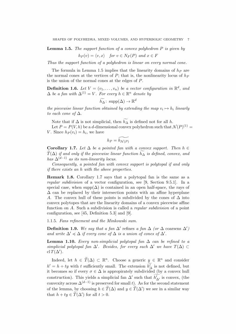
Lemma 1.5. The support function of a convex polyhedron P is given by
hP (v) = 〈v, x〉 for v ∈ NF (P ) and x ∈ FThus the support function of a polyhedron is linear on every normal cone.
The formula in Lemma 1.5 implies that the linearity domains of hP arethe normal cones at the vertices of P ; that is, the nonlinearity locus of hPis the union of the normal cones at the edges of P .
Definition 1.6. Let V = (v1, . . . , vn) be a vector configuration in Rd, and
∆ be a fan with ∆(1) = V . For every h ∈ Rn denote by
h∆ : supp(∆)→ Rd
the piecewise linear function obtained by extending the map vi 7→ hi linearlyto each cone of ∆.
Note that if ∆ is not simplicial, then h∆ is defined not for all h.Let P = P (V, h) be a d-dimensional convex polyhedron such thatN (P )(1) =
V . Since hP (vi) = hi, we have
hP = hN (P )
Corollary 1.7. Let ∆ be a pointed fan with a convex support. Then h ∈T (∆) if and only if the piecewise linear function h∆ is defined, convex, and
has ∆(d−1) as its non-linearity locus.Consequently, a pointed fan with convex support is polytopal if and only
if there exists an h with the above properties.
Remark 1.8. Corollary 1.7 says that a polytopal fan is the same as aregular subdivision of a vector configuration, see [9, Section 9.5.1]. In aspecial case, when supp(∆) is contained in an open half-space, the rays of∆ can be replaced by their intersection points with an affine hyperplaneA. The convex hull of these points is subdivided by the cones of ∆ intoconvex polytopes that are the linearity domains of a convex piecewise affinefunction on A. Such a subdivision is called a regular subdivision of a pointconfiguration, see [45, Definition 5.3] and [9].
1.1.5. Fans refinement and the Minkowski sum.
Definition 1.9. We say that a fan ∆′ refines a fan ∆ (or ∆ coarsens ∆′)and write ∆′ 4 ∆ if every cone of ∆ is a union of cones of ∆′.
Lemma 1.10. Every non-simplicial polytopal fan ∆ can be refined to asimplicial polytopal fan ∆′. Besides, for every such ∆′ we have T (∆) ⊂clT (∆′).
Indeed, let h ∈ T (∆) ⊂ Rn. Choose a generic y ∈ Rn and consider
h′ = h + ty with t sufficiently small. The extension h′∆ is not defined, butit becomes so if every σ ∈ ∆ is appropirately subdivided (by a convex hull
construction). This yields a simplicial fan ∆′ such that h′∆′ is convex, (the
convexity across ∆(d−1) is preserved for small t). As for the second statement
of the lemma, by choosing h ∈ T (∆) and y ∈ T (∆′) we see in a similar way
that h+ ty ∈ T (∆′) for all t > 0.

8 FRANCOIS FILLASTRE AND IVAN IZMESTIEV
The geometric picture behind this argument is that translating facetsof a non-simple polyhedron generically and by small amounts makes thepolyhedron simple without destroying any of its faces.
Definition 1.11. The Minkowski sum of two sets K,L ⊂ Rd is defined as
K + L := x+ y | x ∈ K, y ∈ L
The additive structure on the space of support vectors is related to theMinkowski addition. However, one should be careful when the summandsare not normally equivalent.
Definition 1.12. For two fans ∆1 and ∆2 with the same support denote by∆1 ∧∆2 their coarsest common refinement. Explicitely,
∆1 ∧∆2 = σ1 ∩ σ2 | σi ∈ ∆i, i = 1, 2
Lemma 1.13. Let P and Q be two convex polyhedra such that supp(N (P )) =supp(N (Q)). Then we have:
N (P +Q) = N (P ) ∧N (Q)
Fix V and denote P (h) := P (V, h). Lemma 1.13 implies that in general
P (h+ h′) 6= P (h) + P (h′),
because P (h)+P (h′) can have more facets than P (h+h′). See Figure 3 show-ing fragments of 3-dimensional polyhedra. (However, P (h + h′) ⊃ P (h) +P (h′) holds always.)
P (h+ h′) P (h) P (h′) P (h) + P (h′)
Figure 3. Minkowski addition does not always correspondto the addition of support numbers.
Instead, we have the following.
Lemma 1.14. The support function of the Minkowski sum of two convexbodies is the sum of their support functions:
hK+L = hK + hL
Corollary 1.15. If N (P (h)) 4 N (P (h′)), then P (h) + P (h′) = P (h+ h′).
We also clearly have hλK = λhK and P (λh) = λP (h) for λ > 0. This isfalse for λ < 0. Taking differences of the support functions embeds the spaceof convex polytopes in the vector space of the so called virtual polytopes,see [28], [35].
A subset of a euclidean space is called relatively open, if it is open as asubset of its affine hull. For example, an open half-line in R2 is relativelyopen.

SHAPES OF POLYHEDRA, MIXED VOLUMES, AND HYPERBOLIC GEOMETRY 9
Lemma 1.16. For every polytopal fan ∆, the type cone T (∆) is convex andrelatively open.
The convexity follows from
P (λh+ (1− λ)h′) = λP (h) + (1− λ)P (h′)
for N (P (h)) ' N (P (h′)) and λ ∈ [0, 1], and the relative openness from
h, h′ ∈ T (∆)⇒ h+ εh′ ∈ T (∆),
for ε sufficiently small, whether positive or negative.
1.1.6. Linear inequalities describing a type cone. Let P ⊂ Rd be a d-polytope
with the normal fan ∆. Then P = P (h) for h ∈ T (∆) (we omit V = ∆(1)
from the notation P (V, h)). For every cone σ ∈ ∆ let Fσ(h) be the face ofP (h) with the normal cone σ.
If σ ∈ ∆(d−1), then Fσ(h) is an edge; denote its length by
`∆σ (h) := vol1(Fσ(h))
Of course, all functions `∆σ : T (∆)→ R descend through π : Rn → Rn/ imVto functions on T (∆). However, the proofs of the lemmas in this section
are better written in terms of h than π(h). Due to T (∆) = π(T (∆)) thestatements of the lemmas are easily translated in terms of T (∆).
Lemma 1.17. 1) For every σ ∈ ∆(d−1) and h ∈ T (∆), we have
`∆σ (h) = ‖ grad(hP |ρ1)− grad(hP |ρ2)‖,
where ρ1, ρ2 ∈ ∆(d) are the two full-dimensional cones having σ astheir facet, and hP is the support function of the polytope P = P (h).
2) `∆σ : T (∆)→ R extends to a linear function on span(T (∆)).
Proof. Denote by eσ the unit vector orthogonal to aff(σ) and directed fromρi2 into ρi1 . Then we have
(3) p1 − p2 = `∆σ eσ,
where p1 and p2 are vertices of P with normal cones ρ1 and ρ2, respectively.By Lemma 1.5 we have
hP (v) = 〈v, pα〉 ∀v ∈ ρα, α = 1, 2
and therefore pα = grad(hP |ρα). Substituting this into (3) proves the firstpart of the lemma.
For the second part, choose among the unit length generators of ∆(1)
linearly independent vectors
vj1 , . . . , vjd−1∈ σ
Choose also vi1 ∈ ρ1 \ σ and vi2 ∈ ρ2 \ σ. Then the function hP |ρα , α = 1, 2,is uniquely determined by its values hj1 , . . . , hjd−1
, hiα .
As every set of d+ 1 vectors in Rd is linearly dependent, we have
(4) λ1vi1 + λ2vi1 + µ1vj1 + · · ·+ µd−1vjd−1= 0
for some λα, µβ ∈ R. Besides, λ1, λ2 6= 0. By definition of the supportfunction we have
hi1 = 〈vi1 , p1〉, hjβ = 〈vjβ , p1〉 = 〈vjβ , p2〉, hi2 = 〈vi2 , p2〉

10 FRANCOIS FILLASTRE AND IVAN IZMESTIEV
It follows that
λ1hi1 + λ2hi1 + µ1hj1 + · · ·+ µd−1hjd−1
= λ1〈vi1 , p1〉+ λ2〈vi2 , p2〉+
d−1∑β=1
µjβ 〈vi2 , p2〉
= λ1〈vi1 , p1 − p2〉By substituting (3) we obtain
`∆σ =1
λ1〈vi1 , eσ〉(λ1hi1 + λ2hi1 + µ1hj1 + · · ·+ µd−1hjd−1
),
which shows that `∆σ : T (∆)→ R is a restriction of a linear function.
Remark 1.18. The function `∆σ can be computed as follows. Choose a flagof faces
P ⊃ F1 ⊃ . . . ⊃ Fd−1 = Fσ,
where dimFi = d− i. Project 0 orthogonally to aff(F1). Then the supportnumbers of F1, with respect to the projection of 0, can be written as linearfunctions of the support numbers of P (the coefficients are trigonometricfunctions of the dihedral angles between F1 and adjacent facets). Repeat thisby expressing the support numbers of F2 as linear functions of the supportnumbers of F1, and so on. At the end we obtain the support numbers ofFd−1 (there are two of them, as Fd−1 is a segment) as linear functions of thesupport numbers of P . But the length of Fd−1 is just the sum of these twonumbers.
For d = 3, this computation is done in Appendix A.2.
Note that if ∆ is not simplicial, then we might have several differentchoices for viα , vjβ in the proof of Lemma 1.17, and hence several formulas
for `∆σ in terms of hi. This is due to the fact that, for a non-simplicial ∆,
the set T (∆) does not span the space Rn of support vectors. Thus different
linear functions on Rn have the same restrictions to span(T (∆)).
Lemma 1.19. Let ∆ be a complete pointed polytopal fan with |∆(1)| = n.
1) If ∆ is simplicial, then we have
span(T (∆)) = R∆(1),
2) If ∆ is not simplicial, then
span(T (∆)) = h ∈ R∆(1) | `∆′σ′ (h) = 0 for all σ′ ∈ ∆′(d−1) such that
relintσ′ ⊂ relint ρ for some ρ ∈ ∆(d),where ∆′ is any simplicial refinement of ∆.
Proof. If h ∈ T (∆) for a simplicial ∆, then for every y ∈ Rn the piecewise
linear extension of h + ty with respect to ∆ is convex and has ∆(d−1) asits non-linearity locus, provided that t is sufficiently small. This proves thefirst part of the lemma.
If ∆ is not simplicial, then let us first show
(5) T (∆) ⊂ h ∈ Rn | `∆′σ′ (h) = 0,

SHAPES OF POLYHEDRA, MIXED VOLUMES, AND HYPERBOLIC GEOMETRY 11
with ∆′ and σ′ as in the statement of the lemma. Let h ∈ T (∆). Then
the support function hP = h∆ is linear on ρ, since ρ is a normal cone ofP (h). On the other hand, let ρ′1, ρ
′2 ∈ ∆′ be the d-cones adjacent to σ′. As
ρ′1, ρ′2 ⊂ ρ, we have grad(hP |ρ′1) = grad(hP |ρ′2). As h ∈ cl T (∆′) by Lemma
1.10, the value `∆′
σ′ (h) for h ∈ T (∆) is given by the same formula as for
h ∈ T (∆′). Thus by the first part of Lemma 1.17 we have `∆′
σ′ (h) = 0.
In the other direction, let h ∈ T (∆) and y ∈ ker `∆′
σ′ for all σ′ as in thelemma. We claim that then h + ty ∈ T (∆) for t sufficiently small. Thiswould mean that
h ∈ Rn | `∆′σ′ (h) = 0 ⊂ span(T (∆)),
and thus, together with (5), imply the second part of the lemma. So, take
any ρ ∈ ∆(d) and consider the piecewise linear extension of y with respectto the subdivision of ρ induced by ∆′. This extension is in fact linear, sinceit is linear across all (d − 1)-cones of ∆′ whose relative interiors lie in ρ.This shows that the extension y∆ exists. For t small, the piecewise linearextension of h+ty with respect to ∆ is convex and has the same non-linearity
locus as h∆. Hence h+ ty ∈ T (∆), and we are done.
Remark 1.20. For d = 3, the condition on σ′ in the second part ofLemma 1.19 can be replaced by σ′ /∈ ∆. This is not so for d > 3: ifthe cone σ ∈ ∆(d−1) is not simplicial, then it gets subdivided into simplicialcones σ′i ∈ ∆′(d−1). We thus have σ′i /∈ ∆. However, the correspondingedge lengths are not zero. In fact, the edges Fσ′i(h), which are different for
h ∈ T (∆′), become one edge Fσ(h) for h ∈ T (∆). This means that for
h ∈ T (∆) we have
`∆′
σ′i(h) = `∆
′
σ′j(h)
for any σ′i, σ′j ⊂ σ. Thus these linear equations hold also on span(T (∆)).
However, they don’t enter the description of span(T (∆)) given in the secondpart of Lemma 1.19, as they follow from the other ones (this simply followsfrom the statement of the lemma).
Lemma 1.21. Let ∆ be a complete pointed fan in Rd.If ∆ is simplicial, then T (∆) is the solution set of the following system of
linear inequalities:
T (∆) = h ∈ Rn | `∆σ (h) > 0 for all σ ∈ ∆(d−1)
If ∆ is not simplicial, then T (∆) is the solution set of the following systemof linear equations and inequalities:
T (∆) = h ∈ Rn | `∆σ (h) > 0 for all σ ∈ ∆(d−1), and
`∆′
σ′ (h) = 0 for all σ′ ∈ ∆′(d−1) such that
relintσ′ ⊂ relint ρ for some ρ ∈ ∆(d),
where ∆′ is any simplicial fan that refines ∆.In particular, the closure clT (∆) of the type cone is a convex polyhedral
cone in Rn/ imV .

12 FRANCOIS FILLASTRE AND IVAN IZMESTIEV
Note that the function `∆σ (h) is well-defined only on span(T (∆)). Due
to Lemma 1.19, the above description of T (∆) in the non-simplicial case isunambiguous.
Proof. First, let ∆ be simplicial. Then the inequality `∆σ (h) > 0 just means
that the piecewise linear function h∆ is strictly convex across the (d − 1)-cone σ. It follows that these inequalities are necessary and sufficient for h
to belong to T (∆).Second, let ∆ be non-simplicial. Then, similarly to the proof of Lemma
1.19, the equations `∆′
σ′ (h) = 0 ensure that the linear extension h∆ exists.
And, as in the simplicial case, `∆σ (h) > 0 is equivalent to the strict convexityof this function across σ. The lemma is proved.
1.2. Secondary fans. Everywhere in this section V = (v1, . . . , vn) is alinearly spanning vector configuration in Rd. As usual, V will also stand forthe n× d matrix with rows vi.
1.2.1. The compatibility and the irredundancy domains. As in Section 1.1.3,for an h ∈ Rn denote by P (h) the solution set of the system V x ≤ h. It canhappen that the set P (h) is empty; and even when it is non-empty, it canhappen that some of the inequalities 〈vi, x〉 ≤ hi can be removed withoutchanging P (h). This leads us to consider the following two subsets of Rn.
co(V ) := h ∈ Rn | V x ≤ h is compatible,that is all those h for which P (h) 6= ∅.
ir(V ) := h ∈ Rn | V x ≤ h is compatible and irredundant,where irredundant means that removing any inequality from the systemmakes the solution set bigger.
As in the case with a type cone and a lifted type cone, equation (2)
implies that both co(V ) and ir(V ) are invariant under translation by V t forany t ∈ Rd. Therefore it suffices to study their quotients under the map
(6) π : Rn → Rn/ imV
Definition 1.22. Let V ∈ Rn×d be of rank d. The set
co(V ) := co(V )/ imV
is called the compatibility domain, and the set
ir(V ) := ir(V )/ imV
the irredundancy domain for V , respectively. Further, we denote by clir(V )the closure of ir(V ).
For every polytopal fan ∆ with ∆(1) = V we have T (∆) ⊂ ir(V ), andwe will later see that type cones decompose the interior of ir(V ). Moreover,this can be extended to a subdivision of co(V ), the so called secondary fan.
Most of the material presented here can be found in [26, 27, 5, 6, 9]. Thenotation ir was introduced in [26], meaning “inner region”, but in some laterworks of the same author the terminology was changed to the “irredundancydomain”.

SHAPES OF POLYHEDRA, MIXED VOLUMES, AND HYPERBOLIC GEOMETRY 13
1.2.2. Gale duality, linear dependencies and evaluations. For the moment,we don’t require all vi to have norm 1 (in fact, we even allow vi = 0 orvi = vj for i 6= j).
Definition 1.23. Choose a linear isomorphism Rn/ imV ∼= Rn−d and de-note by V > the matrix representation of the projection (6):
Rd V−→ Rn V >−→ Rn−d
Then the Gale transform or Gale diagram of (v1, . . . , vn) is the collectionof n vectors (v1, . . . , vn) that form the rows of the n× (n− d)-matrix V .
Lemma 1.24. The vector configuration (v1, . . . , vn) is well-defined up to alinear transformation of Rn−d. Besides, if (v1, . . . , vn) is a Gale diagram for(v1, . . . , vn), then also (v1, . . . , vn) is a Gale diagram of (v1, . . . , vn).
Indeed, the uniqueness up to a linear transformation follows from thefreedom in the choice of the isomorphism Rn/ imV ∼= Rn−d. The involutivityof the Gale transform follows by transposing the short exact sequence inDefinition 1.23. It allows also to call the vector configuration (vi) Gale dualto (vi).
Remark 1.25. If V contains the vectors of the standard basis of Rd, thenits Gale dual is very easy to compute:
V =
(EdA
)⇒ V =
(−A>En−d
),
where Ek denotes the k × k-unit matrix.
As an immediate consequence of Definition 1.23 we have
(7) kerV > = im V
The elements of kerV > are the linear dependencies between the vectors(v1, . . . , vn):
λ ∈ kerV > ⇔n∑i=1
λivi = 0,
while the elements of im V are the evaluations of linear functionals on(v1, . . . , vn):
λ ∈ im V ⇔ λi = 〈µ, vi〉 for some µ ∈ Rn−d
Therefore (7) can be phrased as “dependencies of V equal evaluations on V ”.Of course, the same holds with V and V exchanged.
In the next lemma, the rank of a vector configuration means the dimensionof its linear span, so that a rank d configuration is the same as a linearlyspanning configuration. We also use the notation [n] := 1, . . . , n, and forany subset I ⊂ [n] we denote by VI the vector configuration (vi | i ∈ I).
Lemma 1.26. Let V = (v1, . . . , vn) be a rank d configuration of n vectorsin Rd, and let V be its Gale dual.
1) The vector configuration V is positively spanning if and only if thereis µ ∈ Rn−d such that 〈µ, vi〉 > 0 for all i ∈ [n].

14 FRANCOIS FILLASTRE AND IVAN IZMESTIEV
2) Subconfiguration VI is linearly independent if and only if the subcon-figuration V[n]\I has full rank. In particular, VI is a basis of Rd if and
only if V[n]\I is a basis of Rn−d.3) Configuration V contains a zero vector vi = 0 if and only if the
subconfiguration V \vi has rank d−1. In particular, if V is positivelyspanning, then vi 6= 0 for all i.
4) Configuration V contains two collinear vectors vi = cvj (one or bothof which may be zero) if and only if the subconfiguration V \ vi, vjhas rank at most d− 1.
Proof. A configuration V is positively spanning if and only if it has rank dand is positively dependent:
(8) rkV = d,n∑i=1
λivi = 0 so that λi > 0 for all i
Indeed, if (8) holds, then every linear combination of vi can be made positiveby adding a positive multiple of
∑i λivi, so that rkV = d implies that V is
positively spanning. For the inverse implication, express −v1 as a positivelinear combination of vi. On the other hand, by the dependence-evaluationduality (7) a positive dependence of V corresponds to a linear functionalpositively evaluating on V . This proves the first part of the lemma.
The subconfiguration VI is linearly dependent if and only if there is λ ∈Rn, λ 6= 0 such that
n∑i=1
λivi = 0 and λi = 0 for i /∈ I
By the dependence-evaluation duality this is equivalent to the existence ofa non-zero linear functional on Rn−d that vanishes on all vi for i 6= I, whichis equivalent to rk V[n]\I < n− d. This proves the second part of the lemma.
The third part follows from the second: vi = 0 is equivalent to the setvi being linearly dependent, and if rkV = d, then rk(V \ vi) ≥ d − 1.Also, if rk(V \ vi) = d− 1, then −vi /∈ pos(V ).
The fourth part is a direct consequence of the second.
Let V ∈ Rn×d be a vector configuration such that its Gale diagram(v1, . . . , vn) contains no zero vectors (a necessary and sufficient conditionfor this is given in part 3 of Lemma 1.26). The affine Gale diagram is con-structed by choosing an affine hyperplane A ⊂ Rn−d non-parallel to each ofvi and scaling each vi so that
pi = αivi ∈ A
Besides, a point pi is colored black if αi > 0, and white if αi < 0.An affine Gale diagram determines the vector configuration V up to inde-
pendent positive scalings of vi. Indeed, the point pi together with its colordetermines vi up to a positive scaling; and positive scaling vi 7→ βivi of Vcorresponds to positive scaling vi 7→ β−1
i vi of V .
Remark 1.27. By part 1 of Lemma 1.26, a positively spanning vectorconfiguration has an affine Gale diagram consisting of black points only.

SHAPES OF POLYHEDRA, MIXED VOLUMES, AND HYPERBOLIC GEOMETRY 15
By the dependencies-evaluations duality (7), if∑n
i=1 vi = 0, then thevectors vi lie already in an affine hyperplane.
Example 1.28. Let V = (e1, e2, e3,−e1,−e2,−e3) be a configuration of sixvectors in R3. Its Gale dual is V = (e1, e2, e3, e1, e2, e3). The correspondingaffine Gale diagram is shown on Figure 4.
v1
v2
v3
v4
v5
v6
v1 = v4
v2 = v5
v3 = v6
Figure 4. A vector configuration and its affine Gale diagram.
For more details on Gale duality, see [10, 9, 45].
1.2.3. Positive circuits and co(V ).
Definition 1.29. A subset C ⊂ [n] is called a circuit of a vector configura-tion V = (v1, . . . , vn), if VC = (vi | i ∈ C) is an inclusion-minimal linearlydependent subset of V .
An inclusion-minimal linearly dependent set is one that is linearly depen-dent, while each of its proper subsets is not.
The minimality condition implies that a linear dependence λC ⊂ RC be-tween vectors of a circuit C is unique up to a scaling, and that all coefficientsλCi are nonzero. In particular, it makes sense to speak about the signs ofthe coefficients (up to a simultaneous change of all signs).
A circuit C is called positive, if all coefficients of the corresponding lineardependence can be chosen positive:∑
i∈CλCi vi = 0, where λCi > 0 ∀i ∈ C
By the dependence-evaluation duality (7), to a positive circuit C there cor-responds a linear functional µC ∈ Rn−d such that
〈µC , vi〉
> 0, if i ∈ C,= 0, if i /∈ C
Namely, we have λC = V µC . Since V has full rank, µC is well-defined up toa scaling. Besides, the minimality of C implies that V[n]\C is a maximal non-
spanning subconfiguration of V . Such subconfigurations are called cocircuits.We thus have
C is a circuit for V ⇔ [n] \ C is a cocircuit for V
(See also the second part of Lemma 1.26.)

16 FRANCOIS FILLASTRE AND IVAN IZMESTIEV
Theorem 1.30. Let (v1, . . . , vn) be a linearly spanning vector configurationin Rd. Then the compatibility domain co(V ) is a convex polyhedral cone inRn−d. The compatibility domain and its lift co(V ) to Rn can be described inthe following ways.
(9a) co(V ) = Rn+ + imV, where Rn+ = (h1, . . . , hn) | hi ≥ 0 ∀i
(9b) co(V ) = posv1, . . . , vn, where V is the Gale dual of V
(9c) co(V ) =h ∈ Rn | 〈λC , h〉 ≥ 0 for all positive circuits C
(9d) co(V ) =
y ∈ Rn−d | 〈µC , y〉 ≥ 0 for all positive circuits C
Here λC ∈ RC+ are the coefficients of the linear dependence, and µC ∈ Rn−dis the linear functional associated with the circuit C.
Moreover, V is positively spanning if and only if co(V ) is pointed.
Proof. Equation (9a) follows from
x ∈ P (h)⇔ 0 ∈ P (h− V x)⇔ h− V x ∈ Rn+Thus P (h) 6= ∅ if and only if h ∈ Rn+ + imV .
(9a)⇒ (9b): By definition of V we have π(ei) = vi, where ei is a standardbasis vector of Rn. Hence
co(V ) = π(co(V )) = π(Rn+) = pos(v1, . . . , vn)
(9b)⇒ (9d): Represent the cone pos(v1, . . . , vn) as an intersection of half-spaces whose boundary hyperplanes pass through the origin. It suffices totake only those half-spaces whose boundaries are spanned by a subconfig-uration of V . But every such half-space corresponds to a linear functionalvanishing on a maximal non-spanning subset of V and positive otherwise.This yields the representation (9d).
(9d) ⇒ (9c): Due to co(V ) = π−1(co(V )) we have
co(V ) = h ∈ Rn | 〈µC , π(h)〉 ≥ 0Since V : Rn−d → Rn is the adjoint of π and λC = V µC , this corresponds tothe description (9c).
Finally, by Lemma 1.26 V is positively spanning if and only if thereexists a linear functional on Rn−d taking on vi only positive values, whichis equivalent to pos(V ) being pointed.
Note that if pos(V ) is pointed, then V has no positive circuits, and hencethe description (9d) yields co(V ) = Rn−d. This is in full accordance with thedualization of the last statement of the theorem: V is positively spanning ifand only if pos(v1, . . . , vn) is pointed.
Remark 1.31. Parts (9a) and (9b) of Theorem 1.30 are due to McMullen,[26]. See also [9, Theorem 4.1.39].
Equation (9c) can be seen as a version of Farkas Lemma, [45, Chapter 1].Still another interpretation of (9c) is in terms of the support function of
P (h). We have P (h) 6= ∅ if and only if there exists a convex positively
homogeneous function h : Rd → R such that h(vi) ≤ hi. The epigraph

SHAPES OF POLYHEDRA, MIXED VOLUMES, AND HYPERBOLIC GEOMETRY 17
of h is a convex cone containing all points (vi, hi). If we have λ(h) ≥ 0for all positive circuits, then conv(vi, hi) “lies above” 0, and thereforepos(vi, hi) is the epigraph of a convex function.
1.2.4. Hyperbolic circuits and ir(V ). From now on we assume vi 6= 0 andvi 6= λvj for λ > 0.
Our main goal here is to prove an analog of Theorem 1.30 for the spaceir(V ). For this, we need some preliminary work.
Recall that P (h) = x ∈ Rd | V x ≤ h and that h ∈ co(V )⇔ P (h) 6= ∅.Denote
Fi(h) := x ∈ P (h) | 〈vi, x〉 = hi
Lemma 1.32. If h ∈ ir(V ), then Fi(h) 6= ∅.
Proof. By definition, the i-th inequality in V x ≤ h is irredundant if andonly if there exist xout ∈ Rd such that
〈vi, xout〉 > hi, 〈vj , xout〉 ≤ hj ∀j 6= i
Pick xin ∈ P (h). Then for an appropriate convex combination of xin andxout we have 〈vi, x〉 = hi and 〈vj , x〉 ≤ hj for all j 6= i. Thus Fi(h) 6= ∅ andthe lemma is proved.
Remark 1.33. The inverse of Lemma (1.32) does not hold. If Fi(h) 6= ∅and dimFi(h) < dimP (h) − 1, then the i-th inequality is still redundant.Even worse, the i-th inequality can be redundant also when dimFi(h) =dimP (h) − 1, although for this dimP (h) < d is necessary. A concreteexample is the polytope in R2 given by
y ≤ 0, −y ≤ 0, −x ≤ 0, x+ y ≤ 1, x− y ≤ 1
This is a segment with the endpoints (0, 0) and (1, 0), and we have F4 =F5 = (1, 0), which is a facet of P . Nevertheless, both the fourth and thefifth inequalities are redundant.
Note that in the last example removing both redundant inequalities atonce makes the solution set larger. Thus an inclusion-minimal irredundantsubsystem is in general not unique.
The life becomes easier, if we restrict our attention either to the interiorint ir(V ) or to the closure clir(V ) of the irredundancy domain. Note thatthey are the images under the map (6) of the interior and of the closure of
ir(V ), respectively.
Lemma 1.34. We have
(10a) int co(V ) = π(h) | dimP (h) = d
(10b) int ir(V ) = π(h) | dimP (h) = d, dimFi(h) = d− 1 ∀i
(10c) clir(V ) = π(h) | Fi(h) 6= ∅ ∀i
Proof. From (9a) we have int co(V ) = int(Rn+ + imV ). It follows that
h ∈ int co(V )⇔ ∃x : h− V x ∈ intRn+ ⇔ x | V x < h 6= ∅Since x | V x < h = intP (h), and intP (h) 6= ∅⇔ dimP (h) = d, we have(10a).

18 FRANCOIS FILLASTRE AND IVAN IZMESTIEV
Let h ∈ int ir(V ). Since ir(V ) ⊂ co(V ), we have int ir(V ) ⊂ int co(V ), andthus dimP (h) = d. Since every d-dimensional convex polyhedron in Rd isthe intersection of the half-spaces determined by its facets [45, Chapter 2],the i-th inequality is irredundant only if dimFi(h) = d − 1. Thus the lefthand side in (10b) is a subset of the right hand side.
Let us prove that the right hand side of (10b) is a subset of the left handside. First, the right hand side is a subset of ir(V ). Indeed, if dimFi(h) =d − 1, then in a neigborhood of x ∈ relintFi(h) there are points for whichall inequalities in V x ≤ h hold except the i-th, that is the i-th inequalityis irredundant. Further, any small change of h preserves the propertiesdimP (h) = d and dimFi(h) = d − 1, and thus the right hand side is asubset of int ir(V ).
By Lemma 1.32, ir(V ) is a subset of the right hand side of (10c). Sincethe right hand side is closed, it contains also clir(V ). To prove the inverseinclusion, let us show that any h such that Fi(h) 6= ∅ lies in the closure ofint ir(V ). Indeed, for any ε > 0 put h′ = h+ ε1, where 1 = (1, . . . , 1). Thenfor any x ∈ Fi(h) we have
〈vi, x+ εvi〉 = 〈vi, x〉+ ε = hi + ε
〈vj , x+ εvi〉 = 〈vj , x〉+ ε〈vi, vj〉 < hj + ε
(where we assume ‖vi‖ = 1 for all i). It follows that x + εvi ∈ Fi(h′) andthat dimFi(h
′) = d− 1 for all i. Thus h′ ∈ int ir(V ). This proves (10c).
Lemma 1.35. If (v1, . . . , vn) are different unit vectors, then 1 ∈ int ir(V ).In particular, int ir(V ) is non-empty.
The proof is similar to that of the last part of Lemma 1.34: we havevi ∈ Fi(1) and, since 〈vi, vj〉 < 1, we have dimFi(1) = d− 1. The polytopeP (1) is circumscribed about the unit sphere. Its normal fan is related tothe Delaunay tessellation, see Section 4.2.
Note that the assumption ‖vi‖ = 1 is not too restrictive: scaling all vectorsvi by positive factors scales the support numbers hi correspondingly. In thecontext of Gale duality, if vi is replaced by λivi, then it suffices to replacevi by λ−1
i vi.Two more definitions will be needed.
Definition 1.36. Let W = (w1, . . . , wn) be a vector configuration in Rm,where we allow wi = wj for i 6= j. The k-core corek(W ) of W consists ofall y ∈ Rm such that any linear functional that takes a non-negative valueon y takes a non-negative value on at least k entries of W .
(The k-core is also called the set of vectors of depth k, see [44].)If wi 6= 0 for all i, then the 1-core is the positive hull:
core1(W ) = pos(W )
Similarly, the 2-core can be expressed as
core2(W ) =
n⋂i=1
pos(W \ wi)
For example, if for every wi there is a j 6= i such that wj = wi, thencore2(W ) = core1(W ) = pos(W ).

SHAPES OF POLYHEDRA, MIXED VOLUMES, AND HYPERBOLIC GEOMETRY 19
Definition 1.37. A circuit C of a vector configuration V is called hyper-bolic, if one of the coefficients of the corresponding linear dependence ispositive, while the rest are negative. Equivalently, a hyperbolic circuit is anindex subset C = p(C) ∪ C− such that
(11) vp(C) =∑i∈C−
λC−
i vi, where λC−
i > 0 ∀i ∈ C−
and every proper subset of VC = vi | i ∈ C is linearly independent.
A hyperbolic circuit of cardinality 2 consists of two non-zero vectors viand vj such that vi = λvj for λ > 0. In this case any of the indices i and jcan be declared to be p(C). As we assumed at the beginning of this sectionvi 6= λvj for λ > 0, every hyperbolic circuit has cardinality at least 3, andthus the positive index p(C) is well-defined.
Equation (11) means that we are scaling the coefficients of every hyper-bolic circuit C so that
λCp(C) = 1, λCi =
−λC−i , if i ∈ C−
0, if i /∈ C
Due to the dependence-evaluation duality (see (26) and the two equationsfollowing it), to every hyperbolic circuit there corresponds a unique vectorµC ∈ Rn−d such that
〈µC , vp(C)〉 = 1, 〈µC , vi〉 =
−λC−i , if i ∈ C−
0, if i /∈ p(C) ∪ C−
Theorem 1.38. Let (v1, . . . , vn) be a linearly spanning vector configurationin Rd such that
vi 6= 0 ∀i and vi 6= λvj ∀i 6= j
Then the closure clir(V ) of the irredundancy domain is a convex polyhedral
cone in Rn. The set clir(V ) and its lift clir(V ) to Rn can be described in thefollowing ways.
(12a) clir(V ) =
n⋂i=1
(R[n]\i+ + imV ),
where R[n]\i+ = (h1, . . . , hn) | hi = 0, hj ≥ 0 ∀j 6= i.
(12b) clir(V ) =n⋂i=1
pos(V \ vi) = core2(V )
(12c) clir(V ) = h ∈ Rn | 〈λC , h〉 ≥ 0 for all positive circuits C, and
hp(C) ≤ 〈λC−, h〉 for all hyperbolic circuits C
(12d) clir(V ) = y ∈ Rn−d | 〈µC , y〉 ≥ 0 for all positive circuits C, and
〈µC , y〉 ≤ 0 for all hyperbolic circuits C
Moreover, if V is positively spanning, then ir(V ) is pointed.

20 FRANCOIS FILLASTRE AND IVAN IZMESTIEV
Proof. From the definition of Fi(h) it follows that
x ∈ Fi(h)⇔ h− V x ∈ R[n]\i+
Therefore
Fi(h) 6= ∅ ∀i⇔ h ∈n⋂i=1
(R[n]\i+ + imV )
Since clir(V ) = h | Fi(h) 6= ∅ ∀i, we have (12a).
(12a) ⇒ (12b): Since R[n]\i+ is the positive hull of all basis vectors except
ei, we have π(R[n]\i+ ) = pos(V \ vi) and hence
clir(V ) =n⋂i=1
π(R[n]\i+ ) =
n⋂i=1
pos(V \ vi),
(here ∩ and π commute because X + imV is a full preimage under π).
(12b) ⇒ (12c): By definition of irredundancy, h ∈ ir(V ) if and only ifalong with the system V x ≤ h the following n systems:
(13) 〈vi, x〉 > hi, 〈vj , x〉 ≤ hj ∀j 6= i,
i = 1, . . . , n, are compatible. Consequently, h ∈ clir(V ) if and only if allsystems (13) are compatible when > is replaced by ≥. The system (13) can
be rewritten as V (i)x ≤ h(i), where
V (i) = (v1, . . . ,−vi, . . . , vn), h(i) = (h1, . . . ,−hi, . . . , hn)
According to the criterion (9c) of compatibility, we have to consider all
positive circuits of V (i). Each of them is either a positive circuit of V \ vior a hyperbolic circuit of V with i as the positive index. This yields thesystem of linear inequalities in (12c).
(12c) ⇒ (12d): This follows from λC = V µC for any circuit and from ourconvention for hyperbolic circuits, see the paragraph before the theorem.
Finally, if V is positively spanning, then by Theorem 1.30 the cone co(V )is pointed, and hence so is ir(V ) ⊂ co(V ).
Remark 1.39. Again, part (12c) of Theorem 1.38 can be interpreted interms of the support function. Due to (10c) we have
h ∈ clir(V )⇔ hi = h(vi),
where h is the support function of P (h) and ‖vi‖ = 1 is assumed. Since
h is convex, equality hi = h(vi) implies the inequality hi ≤∑
j∈C− λC−j hj
for every hyperbolic circuit C with p(C) = i. In the opposite direction, if
h /∈ clir(V ), then we have hi > h(vi) for some i. This yields a hyperboliccircuit C (where p(C) = i and C− are the indices of the extremal rays ofthe normal cone of P (h) containing vi in its relative interior) that violatesthe linear inequality in the second line of (12c).

SHAPES OF POLYHEDRA, MIXED VOLUMES, AND HYPERBOLIC GEOMETRY 21
1.2.5. Chambers and type cones. Let V = (v1, . . . , vn) be a positively span-ning configuration of n different unit vectors in Rd. By results of the previoussections, every polytope P (h) with outer facet normals vi is represented bya point y = π(h) ∈ Rn−d lying in the interior of the 2-core of the Gale dualconfiguration V = (v1, . . . , vn). We now want to describe how the relativeposition of y with respect to vi determines the combinatorics of the polytope.
By slightly modifying the notation, we will distinguish between the geo-metric normal fan N (P (h)) and the abstract fan ∆ isomorphic to N (P (h)).Here ∆ is a collection of subsets of [n] such that
σ ∈ ∆⇔ pos(Vσ) ∈ N (P (h)),
where as usual Vσ = vi | i ∈ σ.
Lemma 1.40. Let y = π(h) ∈ int core2(V ). Then
(14) pos(Vσ) ∈ N (P (h))⇔ y ∈ relint pos(V[n]\σ)
In other words, vi | i ∈ σ span a normal cone of P (h) if and only if π(h)lies in the relative interior of the cone spanned by vi | i /∈ σ.
Proof. Let Fσ(h) denote the face of P (h) with the normal cone pos(Vσ). Wehave
x ∈ relintFσ(h)⇔ 〈vi, x〉
= hi, if i ∈ σ< hi, if i /∈ σ
⇔ h− V x ∈ relintR[n]\σ+
By applying the projection π, we obtain
Fσ(h) 6= ∅⇔ y ∈ relint pos(V[n]\σ)
But Fσ(h) 6= ∅ is equivalent to pos(Vσ) ∈ N (P (h)), and we are done.
Lemma 1.40 allows to give a very concise description of the type cones ofthe vector configuration V .
Definition 1.41. Let W = (w1, . . . , wn) ⊂ Rm be a vector configuration.Two vectors y1 and y2 are said to lie in the same relatively open chamber,if for every I ⊂ [n] we have
y1 ∈ pos(WI)⇔ y2 ∈ pos(WI)
The closure of a relatively open chamber is called a chamber, and the col-lection of all chambers is called the chamber fan Ch(W ) of W .
Equivalently, a relatively open chamber is an inclusion-minimal intersec-tion of relative interiors of cones generated by W , and the chamber fan isthe coarsest common refinement of all cones pos(WI), I ⊂ [n].
Corollary 1.42. Let ∆ be a complete pointed fan with rays generated by V .Then T (∆) is a relatively open chamber in the chamber fan Ch(V ).
Indeed, two points y1, y2 ∈ Rn−d belong to the same type cone if andonly if the corresponding polytopes have the same normal fan. By Lemma1.40 this is equivalent to y1 and y2 belonging to the same collections ofrelatively open cones pos(VI). Since relatively open and closed cones arerelated through the ∪ and \ operations, this is equivalent to y1 and y2
belonging to the same collections of closed cones.

22 FRANCOIS FILLASTRE AND IVAN IZMESTIEV
Lemma 1.43. Let ∆ be a complete pointed fan with rays generated by V .Then
(15) T (∆) =⋂σ∈∆
relint pos(V[n]\σ) =⋂
ρ∈∆(d)
relint pos(V[n]\ρ)
In particular, the fan ∆ is polytopal if and only if the intersection on theright hand side is non-empty.
Proof. By Lemma 1.40, the left hand side of (15) is a subset of the middle.Clearly, the middle is a subset of the right hand side.
Let us show that the right hand side is a subset of the left hand side. Letπ(h) ∈ relint pos(V[n]\ρ) for all ρ ∈ ∆(d). Since for every i there is ρ ∈ ∆(d)
such that i ∈ ρ, we have⋂ρ∈∆(d)
relint pos(V[n]\ρ) ⊂n⋂i=1
int pos(V[n]\i) = int core2(V ) = int ir(V )
(here rk V[n]\i = n − d for all i allows to replace relint by the absoluteinterior). Hence by (10b) P (h) is a d-polytope with n facets having outernormals v1, . . . , vn and we are in a position to apply Lemma 1.40. It impliesthat pos(Vρ) ∈ N (P (h)) for all ρ ∈ ∆(d). Since the cones pos(Vρ) cover
Rd, the polytope P (h) has no other full-dimensional normal cones, and thusN (P (h)) = ∆.
Note that if the fan ∆ is simplicial, then we have |ρ| = d for all ρ ∈∆(d), and hence |[n] \ ρ| = n − d. According to Lemma 1.26, the vectorconfiguration V[n]\ρ is linearly independent, so that (15) represents T (∆) asa finite intersection of open simplicial d-cones.
Remark 1.44. Chambers of Ch(V ) contained in ∂ clir(V ) ∩ int co(V ) canbe identified with type cones T (∆) for complete pointed fans whose rays aregenerated by proper subsets of V . Chambers contained in int co(V )\clir(V )are linearly isomorphic to T (∆) × intRI+, where I ⊂ [n] is the index set ofredundant inequalities.
Chambers outside int ir(V ) can be studied using the operations of con-traction and deletion on vector configurations. It is easy to see that as aGale dual of V[n]\i (configuration obtained by deletion) one can take pro-
jections of vectors of V[n]\i along vi (configuration obtained by contraction).
According to that, the type cones T (∆) with ∆(1) generated by V[n]\i are the
chambers of the contracted Gale dual V[n]\i. The contraction can be seen as
a central projection in Rn−d from vi. This projection maps those chambersof Ch(V )∩∂ clir(V ) visible from vi to the chambers of Ch(V[n]\i)∩clir(V[n]\i).
Chambers on the boundary of co(V ) correspond to type cones of polytopesof dimension smaller than d. The facet normals of such a polytope P areobtained from V by contraction along vectors vi orthogonal to aff(P ).
Remark 1.45. The chambers fan Ch(V ) is polytopal. Namely, Lemma 1.13and the observation after Definition 1.41 implies that Ch(V ) is the normalfan of the Minkowski sum of representatives of all normal equivalence typeswith facet normals in V . The fan Ch(V ) is called the secondary fan of the

SHAPES OF POLYHEDRA, MIXED VOLUMES, AND HYPERBOLIC GEOMETRY 23
vector configuration V , and any polyhedron that has Ch(V ) as its normalfan is called a secondary polyhedron of V , [5, 6].
If the cone pos(V ) is pointed, then by Lemma 1.26 V is positively span-ning; thus a secondary polyhedron is compact and is called a secondarypolytope. The interest in secondary polytopes was aroused by their applica-tions in algebraic geometry, see the book [16] by Gel’fand, Kapranov, andZelevinsky.
Remark 1.46. Polytopes whose facet normals determine their normal equiv-alence class are called monotypic. For such polytopes,
clir(V ) = clT (∆),
for a unique polytopal fan ∆ with ∆(1) = V . For example, polygonsand polygonal prisms (including parallelepipeds) are monotypic. Monotypicpolytopes are studied in [31].
Remark 1.47. One can show that any convex polyhedral cone is combina-torially (and even affinely) isomorphic to a chamber of some chamber fanCh(W ). By duplicating each vector in W we obtain core2(W ) = pos(W ), sothat all chambers lie in the 2-core. It follows that every convex polyhedralcone can be realized as a type cone of some vector configuration.
Remark 1.48. When the vector configuration V is positively spanning,its Gale dual V can be represented by a point configuration in an affinehyperplane A ⊂ Rn−d, see the paragraphs preceding Remark 1.27. Thenthe linear functionals µ on Rn−d are replaced by affine functions on A, inparticular in the definition of the k-core.
1.2.6. Facets of clir(V ) and truncated polytopes. Recall that C ⊂ [n] is acircuit of V if and only if [n] \C is a cocircuit of V , that is the index set ofa maximal non-spanning subconfiguration. This subconfiguration spans ahyperplane which is the kernel of the linear functional µC , see the beginningof Section 1.2.3.
By (12d), every facet of clir(V ) = core2(V ) is determined by a positive ora hyperbolic circuit of V . The corresponding hyperplane in Rn−d spannedby V[n]\C has all of VC on one of its sides if C is positive, and separates vp(C)
from VC− if C is hyperbolic.Although every facet corresponds to a cocircuit, not every cocircuit (even
not every hyperbolic one) corresponds to a facet of core2(V ), as the followingexample shows.
Example 1.49. The point configuration on Figure 5, right has 3 positiveand 7 hyperbolic cocircuits. None of the positive cocircuits and only 3 ofthe hyperbolic cocircuits determine a facet of its 2-core.
This point configuration is the affine Gale dual of the five vectors in R2
shown on Figure 5, left. Thus the points of the shaded triangle on the rightparametrize the space of pentagons with normals as that on the left.
In the next example every positive and every hyperbolic cocircuit deter-mines a facet of the 2-core.
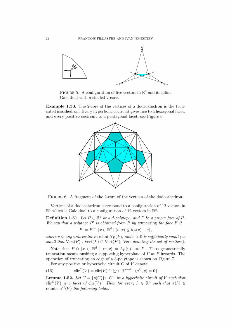
24 FRANCOIS FILLASTRE AND IVAN IZMESTIEV
Figure 5. A configuration of five vectors in R2 and its affineGale dual with a shaded 2-core.
Example 1.50. The 2-core of the vertices of a dodecahedron is the trun-cated icosahedron. Every hyperbolic cocircuit gives rise to a hexagonal facet,and every positive cocircuit to a pentagonal facet, see Figure 6.
Figure 6. A fragment of the 2-core of the vertices of the dodecahedron.
Vertices of a dodecahedron correspond to a configuration of 12 vectors inR4 which is Gale dual to a configuration of 12 vectors in R8.
Definition 1.51. Let P ⊂ Rd be a d-polytope, and F be a proper face of P .We say that a polytope P ′ is obtained from P by truncating the face F if
P ′ = P ∩ x ∈ Rd | 〈v, x〉 ≤ hP (v)− ε,where v is any unit vector in relintNF (P ), and ε > 0 is sufficiently small (sosmall that Vert(P ) \Vert(F ) ⊂ Vert(P ′), Vert denoting the set of vertices).
Note that P ∩ x ∈ Rd | 〈v, x〉 = hP (v) = F . Thus geometricallytruncation means pushing a supporting hyperplane of P at F inwards. Theoperation of truncating an edge of a 3-polytope is shown on Figure 7.
For any positive or hyperbolic circuit C of V denote
(16) clirC(V ) = clir(V ) ∩ y ∈ Rn−d | 〈µC , y〉 = 0Lemma 1.52. Let C = p(C) ∪ C− be a hyperbolic circuit of V such thatclirC(V ) is a facet of clir(V ). Then for every h ∈ Rn such that π(h) ∈relint clirC(V ) the following holds.

SHAPES OF POLYHEDRA, MIXED VOLUMES, AND HYPERBOLIC GEOMETRY 25
P P ′
F
Figure 7. Truncating an edge of a 3-polytope.
1) P (h) is a d-dimensional polytope with outer facet normals V[n]\p(C);2) pos(VC−) ∈ N (P (h));3) P (h− εep(C)) is obtained from P (h) by truncating the face FC−, pro-
vided that ε > 0 is sufficiently small.
Proof. It is easy to show that for a hyperbolic circuit C, relint clirC(V ) ⊂int co(V ). Thus h ∈ relint clirC(V ) implies dimP (h) = d.
Next, if dimP (h) = d, then dimFi(h) = d − 1 is equivalent to the com-patibility of the system
〈vi, x〉 = hi, 〈vj , x〉 < hj ∀j 6= i
which by a standard argument is equivalent to
(17) π(h) ∈ int pos(V[n]\i)
The assumption π(h) ∈ relint clirC(V ) implies that (17) holds for all i 6=p(C), bud doesn’t hold for i = p(C). Hence Fi(h) is a facet of P (h) iffi 6= p(C). This finishes the proof of part 1).
For part 2), observe that clirC(V ) ⊂ pos(V[n]\C), which implies
relint clirC(V ) ⊂ relint pos(V[n]\C)
Then the argument from the proof of Lemma 1.40 implies that pos(VC−)belongs to the normal fan.
Finally, the hyperbolic circuit relation (11) implies vp(C) ∈ relint pos(VC−).Thus by Definition 1.51 P (h− εep(C)) is obtained from P (h) by truncatingFC− .
Lemma 1.53. Let C1 and C2 be two hyperbolic circuits such that clirC1(V )and clirC2(V ) are two facets of clir(V ) intersecting along a codimension 2face of clir(V ). Then for every h ∈ Rn such that π(h) ∈ relint(clirC1(V ) ∩clirC2(V )) the following holds.
1) P (h) is a d-dimensional polytope with outer facet normals V[n]\p1,p2,where pi is the positive index of Ci, i = 1, 2;
2) if p1 /∈ C2 and p2 /∈ C1 (in particular, p1 6= p2), then pos(VC−i) ∈
N (P (h)) for i = 1, 2;3) under the assumptions
p1 /∈ C2, p2 /∈ C1, pos(VC−1 ∪C−2
) /∈ N (P (h))
the polytopes P (h− ε1ep1 − ε2ep2) for all sufficiently small ε1, ε2 > 0are obtained from P (h) by independentely truncating the faces FC−1and FC−2
.
Here truncations of two faces are called independent if the truncated partsare disjoint.

26 FRANCOIS FILLASTRE AND IVAN IZMESTIEV
Proof. The first part is similar to that of Lemma 1.52, if one notes that therelative interior of a codimension 2 face belongs to 2 faces only.
For the second part we have to prove
(18) relint(clirC1(V ) ∩ clirC2(V )) ⊂ relint pos(V[n]\Ci) for i = 1, 2
In other words, for two cones clirC1(V ) ⊂ pos(V[n]\C1) of the same dimen-
sion we have to show that the facet clirC1(V ) ∩ clirC2(V ) of the former isnot contained in a facet of the latter (and the same with indices 1 and 2 ex-changed). The ray R+vp2 is an extreme ray of pos V and, since p2 ∈ [n]\C1,
also of pos(V[n]\C1). Since R+vp2 and clirC1(V ) lie on different sides from
the facet clirC1(V ) ∩ clirC2(V ), this facet cannot be contained in a facet ofpos(V[n]\Ci), and we are done.
Finally, the third part is true because pos(VC−1 ∪C−2
) /∈ N (P (h)) implies
that the faces FC−1and FC−2
of P (h) are disjoint. Hence all small truncations
of those faces are independent. The lemma is proved.
1.3. Examples. In the following examples of vector configurations V we an-alyze the closure clir(V ) of the irredundancy domain and its decompositioninto type cones. We are using both the direct approach (“what happenswhen the facets of a polytope are translated”) and the more formal one,through Gale diagram, circuits, and the chamber fan.
1.3.1. Parallelepipeds with fixed face directions. Let (v1, v2, v3) be a basis ofR3, put vi+3 = −vi, i = 1, 2, 3, and consider the resulting configuration Vof six vectors in R3.
All polyhedra with facet normals V are normally equivalent: they areparallelepipeds with face normals ±vi. The normal fan ∆ is generated by ahyperplane arrangement spanned on the vectors v1, v2, v3.
The lifted type cone T (∆) consists of h ∈ R6 that satisfy
(19) h1 + h4 > 0, h2 + h5 > 0, h3 + h6 > 0
By identifying R6/ imV with h ∈ R6 | h4 = h5 = h6 = 0, we obtain
clT (∆) ∼= (h1, h2, h3) | hi ≥ 0, i = 1, 2, 3
The extreme rays of the cone clT (∆) correspond to degeneration of a paral-lelepiped into a segment parallel to one of the three vectors v1× v2, v2× v3,v3 × v1.
The Gale diagram of V has the property vi+3 = vi, i = 1, 2, 3. This fitstogether with the fact co(V ) = ir(V ): the second core of a vector configu-ration where each vector is repeated twice is its convex hull, see Definition1.36 and equation (12b). The facets of the cone (19) correspond to the threepositive circuits 1, 4, 2, 5, and 3, 6.
1.3.2. Polygons. Let α := (α1, . . . , αn) with 0 < αi < π be an n-tuple ofreal numbers such that
∑i αi = 2π. Let v1, . . . , vn ∈ R2 be unit vectors
such that the angle from vi to vi+1 equals αi+1 (of course, the indices aretaken modulo n). This determines a fan ∆ in R2. The fan is polytopal sincefor every collection of positive numbers a1, . . . , an such that
∑ni=1 aivi = 0
there is a convex polygon with edge lengths ai and edge normals vi. We will

SHAPES OF POLYHEDRA, MIXED VOLUMES, AND HYPERBOLIC GEOMETRY 27
denote T (∆) by T (α). Note that clT (α) is a pointed (n − 2)-dimensionalcone. To avoid dealing with trivial cases, below we assume n ≥ 5.
By Lemma 1.21, every facet of T (α) corresponds to vanishing of an edge:`i = 0. This is possible without making any other edges to disappear if andonly if αi + αi+1 ≤ π. It follows that clT (α) has n, n − 1 or n − 2 facets.Denote by Ti the facet `i = 0 of clT (α). If j /∈ i, i− 1, i + 1 then Ti andTj meet along a codimension 2 facet. Otherwise, Ti and Ti+1 meet if andonly if αi + αi+1 + αi+2 < π.
An extreme ray e of clT (α) corresponds to triangles with fixed edge nor-mals vi1 , vi2 , vi3 . This means that `j = 0 for all j /∈ i1, i2, i3 while `iα 6= 0.Thus e is contained in exactly n − 3 facets, and hence T (α) is simple. Itfollows that clT (α) is the cone over an (n − 3)-dimensional polytope thatis either a simplex, or truncated simplex, or doubly truncated simplex. See[4] for more details and the case of non-convex polygons.
In the Gale diagrams language, the cone clT (α) is the 2-core of the Galedual V . Figure 5 shows an example for n = 5, where this cone has threefacets.
1.3.3. Polygonal prisms. Embed R2 as a coordinate plane in R3 and add tothe vectors v1, . . . , vn ∈ R2 from the preceding example the third basis vectorand its inverse: vn+1 = e3 and vn+2 = −e3. This new vector configurationV + determines only one pointed fan, namely the normal fan of a prism overan n-gon. Denote this fan by ∆+, and its type cone by T+(α). Then wehave
(h, hn+1, hn+2) ∈ T+(α)⇔ h ∈ T (α) and hn+1 + hn+2 > 0
Thus T+(α) is a product of T (α) with a half-space. It follows that
T+(α) = T (α)× R+
The new extreme ray 0 × R+ corresponds to degeneration of the prisminto a segment parallel to e3.
The Gale diagram of V + lives in the space Rn−1 which is one dimensionhigher than that for V . It is easy to see that V + is obtained from V byadding two equal vectors vn+1 = vn+2 = en−1. It follows that the 2-core ofV ∪en−1, en−1 is the pyramid over the 2-core of V , which yields the sameresult as above.
1.3.4. Triangular bipyramid. Let u1, u2, u3 ∈ R2 be outward unit normalsto the edges of a regular triangle. Choose λ, µ > 0 such that λ2 + µ2 = 1and consider the following six vectors in R6:
(20)v1 = λu1 + µe3, v2 = λu2 + µe3, v3 = λu3 + µe3
v4 = λu1 − µe3, v5 = λu2 − µe3, v6 = λu3 − µe3
The 3-polytope V x ≤ 1 is a bipyramid over a triangle, see Figure 8. Theright half of the picture schematically shows the normal fan of the bipyramid(as a stereographic projection of the intersection of the normal fan with thesphere).
By translating the faces of the bipyramid, we can split its four-valentvertices into pairs of three-valent vertices. For the spherical section of thenormal fan this means subdividing quadrilaterals by their diagonals. Let

28 FRANCOIS FILLASTRE AND IVAN IZMESTIEV
v2
v3
v4
v5v1
v4v6
v3
v1
v6
Figure 8. The bipyramid over triangle and its normal fan.
us apply the Gale diagram technique to study the arrangement of the typecones that correspond to different combinatorial types.
Let V be the 6 × 3-matrix with rows vi. We have to find a 6 × 3-matrixV of rank 3 whose columns are orthogonal to those of V . The matrix V isunique up to a multiplication from the right with an element of GL(R, 3).Since the vectors v4, v5, v6 form a basis of R3, the vectors v1, v2, v3 must dothe same (see Lemma 1.26). Thus we may assume
v1 = (1, 0, 0), v2 = (0, 1, 0), v3 = (0, 0, 1)
The remaining entries of V can be easily determined from the orthogonalitycondition between the columns of V and V :
V =
λu1 µλu2 µλu3 µλu1 −µλu2 −µλu3 −µ
V =
1 0 00 1 00 0 1−1
323
23
23 −1
323
23
23 −1
3
Recall that the map
V > : Rn → Rn−d ∼= Rn/ imV
projects the space of support vectors h to its quotient by translations ofthe polytope P (h) (see equation (2) and Definition 1.23). We identify Rn−dwith a subspace of Rn via a right inverse ι of V >. In our case, we can putι(ei) = ei for i = 1, 2, 3, so that Rn−d = R3 is identified with the subspaceh4 = h5 = h6 = 0 of R6. Geometrically this corresponds to fixing the lowervertex of the bipyramid at the origin and varying only the heights h1, h2, h3.
The rows of V are the coordinates of six vectors forming the Gale diagramof V . Since all of them lie in the subspace h1 + h2 + h3 > 0, we can con-veniently draw the affine Gale diagram by intersecting the cones generatedby V with the affine hyperplane h1 + h2 + h3 = 1, see Figure 9, left. (By alucky coincidence, the vectors vi lie in this plane.)
Figure 9, right, shows the quotients co(V ) and ir(V ) of the compatibilitydomain and of the irredundancy domain. According to (9b), co(V ) is thepositive hull of V , which in the affine Gale diagram becomes the convex hull.According to (12b), ir(V ) is the 2-core of V , which is shown as a shadedhexagon on Figure 9.
It is also possible to interpret Figure 9, right, in terms of positive andhyperbolic circuits, see equations (9c) and (12c). The six positive circuits

SHAPES OF POLYHEDRA, MIXED VOLUMES, AND HYPERBOLIC GEOMETRY 29
v1 = (1, 0, 0)
v2 = (0, 1, 0)
v4 = (− 13 ,
23 ,
23 )
v5 = ( 23 ,−
13 ,
23 )
v3 = (0, 0, 1) v1
v2
v5
v6
v3
v6 = ( 23 ,
23 ,−
13 ) v4
Figure 9. The Gale diagram of the face normals of a tri-angular bipyramid (left); the compatibility and the irredun-dancy domains (right).
of the vector configuration V are obtained from
v1 + 2v2 + v4 + 2v6 = 0
by the action of the dihedral group. This particular circuit leads accordingto (9b) to the inequality h1 + 2h2 ≥ 0 in the h4 = h5 = h6 = 0 space, whichdetermines the half-space containing vectors v3 and v5 in its boundary. Theother five edges of the big hexagon on Figure 9 correspond to the other fivepositive circuits.
The lines bounding the irredundancy domain correspond to hyperboliccircuits (in this example, the inequalities in (12c) generated by the positivecircuits turn out to be redundant). For example, the line highlighted onFigure 9 corresponds to the circuit
(21) v1 = 2v2 + 2v3 + 3v4,
The principle “evaluations on V correspond to dependencies in V ” (see (7))allows to read off the signature of the circuit from the position of the line.Since the line separates v1 from v2, v3, and v4, the coefficient at v1 hasthe sign opposite to those at v2, v3, and v4; the points lying on the linecorrespond to zero coefficients.
In order to obtain the chamber fan of the vector configuration V , onehas to draw the diagonals v1v4, v2v5, and v3v6, in addition to those drawnalready on Figure 9. The chambers in the interior of the 2-core are the typecones of V . Figure 10 shows the subdivision of clir(V ) into chambers anddescribes the faces of one of the full-dimensional type cones.
For any point h ∈ clir(V ) (recall that we identified R3 with a subspaceof R6 by putting h4 = h5 = h6), the combinatorics of the correspondingpolytope can be read off from the diagram. By Lemma 1.40, the normalfan of P (h) contains the cone pos(VI) (equivalently, facets with normalsvi | i ∈ I intersect along a face) if and only if h lies in the relative interiorof the positive hull of V[6]\I . For example, since the type cone highlightedon Figure 10 lies in relint posv1, v2, v5, the corresponding fan ∆ containsthe cone spanned by v3, v4, v6. The normal fan corresponding to this type

30 FRANCOIS FILLASTRE AND IVAN IZMESTIEV
h1=h2
h2 =
h3
h 1=
2(h 2
+h 3
)
h3
=0
h1 ≥ h2 ≥ h3 ≥ 0
Figure 10. A type cone.
cone is shown in the center of the Figure 11. This normal fan is simplicial,since the type cone is full-dimensional (compare Lemma 1.19).
The other fans on Figure 11 are associated with the faces of the depictedtype cone. Note that the fans corresponding to boundary points of clir(V )aren’t using all of the vertices vi, compare Lemma 1.52.
1
2
4
5
63
Figure 11. The fans corresponding to the faces of a type cone.
Crossing from one fully-dimensional type cone to an adjacent one corre-sponds to a “flip”, see Figure 12. The edge F35 becomes replaced by theedge F26, compare the description of the faces of the type cones throughvanishing edge lengths, Lemma 1.21. From a different point of view, bound-aries between full-dimensional type cones correspond to (non-positive andnon-hyperbolic) circuits of the vector configuration V . A circuit of this formcorresponds to contracting an edge of the polytope, see equation (4). Thereare three such circuits:
v1 + v5 = v2 + v4, v2 + v6 = v3 + v5, v3 + v4 = v1 + v6,
and they correspond to the hyperplanes
h1 + h5 = h2 + h4, h2 + h6 = h3 + h5, h3 + h4 = h1 + h6,

SHAPES OF POLYHEDRA, MIXED VOLUMES, AND HYPERBOLIC GEOMETRY 31
or, in our picture to the lines
h1 = h2, h2 = h3, h3 = h1
v2
v3v4
v5
v6
v1
v2
v3v4
v5
v6
v1
v2
v3v4
v5
v6
v1
2, 3, 52 6
2, 3, 6
2, 5, 62 6
33, 5, 6
55
3
62
5
3
Figure 12. The flip 2, 3, 5, 3, 5, 6 2, 3, 6, 2, 5, 6.
The fan on Figure 13, left, is not polytopal. Indeed, since it containsposv1, v6, posv2, v4, and posv3, v5, the corresponding point π(h) mustlie in the intersection
relint posv2, v3, v4, v5 ∩ relint posv1, v3, v5, v6 ∩ relint posv1, v2, v4, v6,
which is empty. Similarly, the other two fans on Figure 13 are also non-polytopal. (One can also refer to Figure 11, where all, up to symmetry,polytopal fans with the 1-skeleton in V are shown.)
Figure 13. Examples of non-polytopal fans.

32 FRANCOIS FILLASTRE AND IVAN IZMESTIEV
2. Mixed volumes
2.1. The examples, continued. We continue the examples considered inSection 1.3. Motivated by the observation of Bavard and Ghys [4] thatthe area of convex polygons as a function of their support numbers hi is aquadratic form of hyperbolic signature, we are looking at the surface areaof 3-dimensional polytopes.
2.1.1. Parallelepipeds with fixed face directions. The surface area of the par-allelepiped x | 0 ≤ 〈x, vi〉 ≤ hi, i = 1, 2, 3 equals
area(h) =2
D(h1h2 + h2h3 + h3h1),
where D = |det(v1, v2, v3)|. This is a quadratic form of signature (+,−,−).
2.1.2. Polygons. The area of a polygon with support vector h ∈ T (α) ⊂ Rnequals
area(h) =1
2
∑i
hi`i(h),
where the edge length `i(h) is a linear function of h. Thus area(h) is aquadratic form. The associated symmetric bilinear form is
(22) area(h, k) =1
2
∑i
hi`i(k) =1
2
∑i
ki`i(h),
due to ∂ area(h)∂hi
= `i(h) that follows from a simple geometric argument.
The quadratic form area(h) has signature (+, 0, 0,−, . . . ,−). This canbe proved by induction on the number of edges of the polygon as in [4],or using the Minkowski inequality [37, p. 321] in the plane. See also [20,Lemma 2.14].
2.1.3. Polygonal prisms. Denote by area+(h+) the surface area of a prism(h, hn+1, hn+2) over the n-gon. Here vn+1 and vn+2 are as in Section 1.3.3.Then we have
area+(h+) = 2 area(h) + (hn+1 + hn+2) per(h)
= 2 area(h) + 2(hn+1 + hn+2) area(1, h)
with the associated symmetric bilinear form
area+(h+, k+) = 2 area(h, k)
+ (hn+1 + hn+2) area(1, k) + (kn+1 + kn+2) area(1, h)
The restriction of area+ to Rn is 2 area that by the above results hassignature (+, 0, 0,−, . . . ,−). The vector (0,−1, 1) belongs to the kernel ofarea+ (it corresponds to vertical translation). The vector (1,−1,−1) isorthogonal to Rn ⊂ Rn+2 with respect to area+, and is negative. Thisimplies that area+ has signature (+, 0, 0, 0,−, . . . ,−).

SHAPES OF POLYHEDRA, MIXED VOLUMES, AND HYPERBOLIC GEOMETRY 33
2.1.4. Triangular bipyramid. Let v1, . . . , v6 ∈ R3 be as in 1.3.4. The combi-natorics of a polyhedron P (h) with face normals (vi) depends on h. Let uscompute area(∂P (h)) for the type cone ∆ shaded on Figure 10.
The normal fan of P (h) (the triangulation in the center of Figure 11)shows that P (h) is a doubly truncated tetrahedron, see Figure 14. We have
P (h) = (Σ1 \ Σ2) \ Σ3,
whereΣ1 := x ∈ R3 | 〈vi, x〉 ≤ hi, i ∈ 2, 3, 4, 5Σ2 := x ∈ R3 | 〈vi, x〉 ≤ hi, i ∈ 2, 3, 4, 〈v1, x〉 ≥ h1Σ3 := x ∈ R3 | 〈vi, x〉 ≤ hi, i ∈ 3, 4, 5, 〈v6, x〉 ≥ h6
The surface area of a tetrahedron with fixed face normals is proportionalto the squared length of any of its edges, and the edge length is a linearfunction of the support vector. Thus we have
area(∂Σ1) = f21 (h),
for some linear function f1. We have f1(h) = 0 if and only if the hyperplanesHi, i ∈ 2, 3, 4, 5 pass through a common point, that is iff the system〈vi, x〉 = hi has a solution. Since v2 + 2v3 + 2v4 + v5 = 0, a solution existsif and only if h2 + 2h3 + 2h4 + h5 = 0. By restricting to h4 = h5 = h6 = 0as we have done in Section 1.3.4, we obtain
area(∂Σ1) = c1(h2 + 2h3)2
for some c1 > 0.
F6
F1
Σ3
Σ2
F4
F3
Figure 14. Representing P (h) as a truncated tetrahedron.
Next, observe that
area(∂Σ1 \ Σ2) = area(∂Σ1)− area(F2(Σ2))− area(F3(Σ2))
− area(F4(Σ2)) + area(F1(Σ2))
All quantities area(Fi(Σ2)) are proportional to the square of a linear functionf2(h) that vanishes when the tetrahedron Σ2 degenerates. Similarly to theprevious paragraph, using (21), we find f2(h) = h1 − 2h2 − 2h3 − 3h4, andhence
area(∂Σ1 \ Σ2) = c1(h2 + 2h3)2 − c2(h1 − 2h2 − 2h3)2

34 FRANCOIS FILLASTRE AND IVAN IZMESTIEV
Here c2 > 0 because the sum of areas of three faces of a tetrahedron is biggerthan the area of its fourth face.
Finally, cutting off the tetrahedron Σ3 yields
area(∂P (h)) = q∆(h) := c1f21 − c2f
22 − c3f
23 , c1, c2, c3 > 0,
where
f1(h) = h2 + 2h3, f2(h) = h1 − 2h2 − 2h3, f3(h) = h3.
Since f1, f2, f3 are linearly independent, quadratic form q∆(h) has signature(+,−,−).
2.2. Mixed volumes and quadratic forms.
2.2.1. Definition and basic properties of mixed volumes. Minkowski [32] hasshown that the volume behaves polylinearly with respect to the Minkowskiaddition and positive scaling. Namely, for any compact convex bodiesK1, . . . ,Km ⊂ Rd there exist real numbers ci1...id , 1 ≤ iα ≤ m such that
(23) vol(λ1K1 + · · ·+ λmKm) =∑iα∈[m]
ci1...idλi1 · · ·λid
holds for all λ1, . . . , λm ≥ 0. The coefficients ci1...id are uniquely determinedby the bodies Ki1 , . . . ,Kid if we require that they are symmetric with respectto permutations of indices: cϕI = cI for all ϕ ∈ Sm.
Definition 2.1. The coefficient ci1...id in (23) is called a mixed volume anddenoted by vol(Ki1 , . . . ,Kid).
Clearly, vol(K, . . . ,K) = K. For more details on mixed volumes, see [37,Chapter 5] and [10, Chapter IV].
Example 2.2. A special case of (23) is the Steiner formula
vol(K + ρB) =
d∑i=0
(d
i
)ρiWi(K)
where B is the unit ball. The coefficients Wi(K) = vol(K, . . . ,K︸ ︷︷ ︸d−i
, B, . . . , B︸ ︷︷ ︸i
)
are called quermassintegrals of K. We have W0(K) = vol(K), W1(K) =1d area(∂K), Wd(K) = vol(B). For a polytope P we have
Wi(P ) = cd,i∑
F∈Fd−i(P )
vold−i(F ) · |NF (P )|
for some constant cd,i independent of P , where the sum ranges over all(d − i)-faces of P and |NF (P )| denotes the angular measure of the normalcone NF (P ) ⊂ Rd.
The following properties of mixed volumes will be needed in the sequel.
• Mixed volume is multilinear with respect to the Minkowski addition:
vol(λK + µL,K) = λ vol(K,K) + µ vol(L,K) for λ, µ ≥ 0,
where K = (K1, . . . ,Kd−1).

SHAPES OF POLYHEDRA, MIXED VOLUMES, AND HYPERBOLIC GEOMETRY 35
• Mixed volume is monotone under inclusion: vol(K,K) ≥ vol(L,K) ifK ⊃ L. In particular,
(24) vol(K1, . . . ,Kd) ≥ 0
More precisely, we have the following [37, Theorem 5.1.7].
Theorem 2.3. The inequality in (24) is strict if and only if there are seg-ments si ⊂ Ki, i = 1, . . . , d with linearly independent directions.
In particular, the inequality (24) is strict if dimKi = d for all i.
2.2.2. Alexandrov-Fenchel inequalities and signatures of quadratic forms.Fix convex bodies K1, . . . ,Kd−2 ⊂ Rd and denote K := (K1, . . . ,Kd−2).Then the function
(25) volK : K 7→ vol(K,K,K)
on the set of convex bodies in Rd possesses the valuation property:
(26) volK(K ∪ L) + volK(K ∩ L) = volK(K) + volK(L),
provided that K ∪ L is convex. Besides, it is homogeneous of degree 2:
(27) volK(λK) = λ2 volK(K)
This follows quite easily from the corresponding properties of the volume,see [30].
Let ∆ be a complete polytopal fan in Rd. Due to the multilinearity ofthe mixed volume and compatibility of the Minkowski addition with the
linear structure of T (∆) (Corollary 1.15), the function volK on T (∆) is arestriction of a quadratic form.
Definition 2.4. Given a collection K = (K1, . . . ,Kd−2) of convex bodiesand a complete polytopal fan ∆, denote by qK,∆ the unique quadratic form
on span(T (∆)) such that
qK,∆(h) = vol(P (h), P (h),K) for h ∈ T (∆)
The following properties of qK,∆ are immediate.
• The kernel of qK,∆ contains imV and thus has dimension at least d.• If dimKi = d for all i = 1, . . . , d − 2, then qK,∆(h) > 0 for all
h ∈ T (∆).
The following theorem [1, 37] tells us more about the signature of q∆.
Theorem 2.5 (Alexandrov-Fenchel inequalities). The inequality
(28) vol(K,L,K)2 ≥ vol(K,K,K) vol(L,L,K)
holds for all compact convex bodies K,L,K1, . . . ,Kd−2.
Equation (28) basically says that the Gram matrix of the restriction of
qK,∆ to any 2-dimensional subspace spanned by two vectors from T (∆) hasa non-positive determinant. This is used in the proof of the following lemma(compare with [21, Appendix A.3]).
Lemma 2.6. Let K = (K1, . . . ,Kd−2) consist of d-dimensional convex bod-ies. Then for every polytopal fan ∆ the quadratic form qK,∆ has the followingproperties.

36 FRANCOIS FILLASTRE AND IVAN IZMESTIEV
1) The positive index of qK,∆ equals 1.2) We have dim ker qK,∆ = d if and only if the Alexandrov-Fenchel in-
equality for
K = P (h), L = P (h′), 0 6= h, h′ ∈ T (∆)
holds with equality only when h′ − λh ∈ imV for some λ.
Proof. Due to qK,∆(h) > 0 for all h ∈ T (∆), we have ind+(qK,∆) ≥ 1.If ind+(qK,∆) ≥ 2, then there exists a positive vector x in the orthogonalcomplement to h with respect to qK,∆. For a sufficiently small ε we have
h′ := h+ εx ∈ T (∆),
since T (∆) is relatively open, see Lemma 1.16. It follows that the restrictionof qK,∆ to span(h, x) = span(h, h′) is positive definite, and hence the Grammatrix of qK,∆ with respect to h, h′ has a positive determinant. Thus
qK,∆(h, h)qK,∆(h′, h′)− qK,∆(h, h′)2 > 0,
which contradicts the Alexandrov-Fenchel inequality. Hence ind+(qK,∆) = 1,and the first part of the lemma is proved.
For 0 6= h, h′ ∈ T (∆) the condition h′ − λh /∈ imV for all λ is equivalentto
(29) dimE = 2 and E ∩ imV = 0,where E = span(h, h′). Assume that dim ker qK,∆ = d, that is ker qK,∆ =imV . Then (29) implies that the restriction of qK,∆ to E is non-degenerate,thus the determinant of its Gram matrix doesn’t vanish. It follows that theAlexandrov-Fenchel inequality for h, h′ is strict.
In the opposite direction, if dim ker qK,∆ ≥ d+ 1, then
dim spanh, ker qK,∆ ≥ d+ 2,
which allows us to choose E ⊂ spanh, ker qK,∆ transversal to imV . Thenthe restriction of qK,∆ to E is degenerate, and representing E as span(h, h′)
for h′ ∈ T (∆), we see that the Alexandrov-Fenchel inequality for h, h′ holdswith equality. The lemma is proved.
2.2.3. Quadratic forms of nullity d. The condition h′ − λh ∈ imV meansthat K = P (h) and L = P (h′) are homothetic. But equality in (28) cantake place also for non-homothetic K and L.
Example 2.7. For d = 3, let K = Σ be a tetrahedron, and L = Σ \ Σ1 atruncated tetrahedron, where we assume that the common vertex of Σ andΣ1 lies at the coordinate origin. Then it can be shown (for example, withthe help of the support function) that
λK + µL = (λ+ µ)Σ \ µΣ1
See also Figure 15 for the 2-dimensional case.It follows that
vol(λK + µL) = (λ+ µ)3 vol(Σ)− µ3 vol(Σ1)
= λ3 vol(Σ) + 3λ2µ vol(Σ) + 3λµ2 vol(Σ) + µ3 vol(Σ \ Σ1),

SHAPES OF POLYHEDRA, MIXED VOLUMES, AND HYPERBOLIC GEOMETRY 37
Figure 15. Illustration for Example 2.7.
and hencevol(L,L,K) = vol(L,K,K) = vol(K)
Therefore vol(K,L,K)2 = vol(K,K,K) vol(L,L,K), although K and L arenot homothetic.
A complete characterization of the equality case in the Alexandrov-Fenchelinequality is still missing, see [37, Section 6.6], but there are some partialresults. Roughly speaking, if equality holds for some non-homothetic K andL, then their normal fans are more complicated than those of K1, . . . ,Kd−2.
Theorem 2.8. If K = (B, . . . , B), where B is the unit ball, and dimK =dimL = d, then the Alexandrov-Fenchel inequality (28) holds with equalityonly if K and L are homothetic.
This was proved by Kubota [25], see also [37, Theorem 6.6.2]. Moregenerally, Ki, i = 1, . . . , d− 2 may be any smooth convex bodies.
In view of Example 2.2, Theorem 2.8 implies
Corollary 2.9. For d = 3, the function h 7→ area(∂P (h)) restricted to any
type cone T (∆) is a quadratic form q∆ of signature (+, 0, 0, 0,−, . . . ,−).For d > 3, the (d− 2)-nd quermassintegral
h 7→∑
σ∈∆(d−2)
|σ| · area(Fσ)
restricted to any type cone T (∆) is a quadratic form q∆ of signature (+, d ·0,−, . . . ,−).
The form q∆ in this corollary is proportional to qK,∆, whereK = (B, . . . , B).The next result is a reformulation of [37, Theorem 6.6.20].
Theorem 2.10. Let K = K1, . . . ,Kd−2 be a collection of normally equiva-lent simple polytopes with the normal fan ∆0. Then the Alexandrov-Fenchelinequality (28) holds with equality if and only if after applying a suitablehomothety to K or L we have
hK(v) = hL(v) for all v ∈ ∆(2)0
Corollary 2.11. Let K = K1, . . . ,Kd−2 be a collection of normally equiv-alent simple polytopes with the normal fan ∆0. Then the quadratic form qK,∆
has signature (+, d · 0,−, . . . ,−) if ∆(1) ⊂ ∆(2)0 .

38 FRANCOIS FILLASTRE AND IVAN IZMESTIEV
In particular, the assumption of the Corollary 2.11 is fulfilled when ∆(1) =
∆(1)0 , that is when Ki and K = P (h) have the same sets of the outward facet
normals.
Corollary 2.12. Let V be a vector configuration in R3, and let h0 ∈int ir(V ). Then the weighted sum of face areas
h 7→n∑i=1
h0i area(Fi(h))
restricts on every type cone T (∆) with ∆(1) = V to a quadratic form ofsignature (+, 0, 0, 0,−, . . . ,−).
Proof. Since
vol(P (h), P (h), P (h0)) =1
3
n∑i=1
h0i area(Fi(h)),
(see [37, 10]), the quadratic form in the corollary is proportional to qP (h0),∆.
Polytopes P (h0) and P (h) have the same sets of face normals: ∆(1)0 =
∆(1) = V . If P (h0) is simple, then the remark after Corollary 2.11 applies.If P (h0) is not simple, then it can be made simple by truncating verticesthat have more than three adjacent edges. The quadratic form does notchange (similarly to Example 2.7), while the normal fan of K1 becomes onlyricher. Thus, by Corollary 2.11, the form has the right signature.
Example 2.13. We know (Lemma 1.35) that 1 ∈ int ir(V ). For h0 = 1the quadratic form in Corollary 2.12 is simply the surface area of P , thatis coincides with the quadratic form from the first part of Corollary 2.9.Geometrically, P (1) is the circumscribed polytope. We thus have
vol(P (h), P (h), P (1)) = vol(P (h), P (h), B),
which is another example of non-strict monotonicity of mixed volumes, com-pare Theorem 2.3 and the paragraph before it.
Remark 2.14. For every simplicial polytopal fan ∆ in Rd there exists ahomogeneous polynomial Z∆ of degree d such that
vol(P (h)) = Z∆(h) for all h ∈ T (∆)
The mixed volume of polytopes with the normal fan ∆ is given by thepolarization of the polynomial Z∆. (In fact, the existence of development(23) is usually proved through approximation of Ki by normally equivalentsimple polytopes.)
It follows that the quadratic form qK,∆ for K = (P (h0), . . . , P (h0)) withh0 ∈ ∆ is proportional to the Hessian of vol(P (h)) at h = h0. By Corollary2.11, this Hessian is non-degenerate modulo translations. This is relatedto the uniqueness part of the Minkowski problem for polytopes; besides,knowing the signature of the Hessian allows to prove the existence part.By duality, this is related to the infinitesimal rigidity of convex polytopes,[21, 20].

SHAPES OF POLYHEDRA, MIXED VOLUMES, AND HYPERBOLIC GEOMETRY 39
3. Hyperbolic geometry
3.1. From type cones to hyperbolic polyhedra. Let ∆ be a simplicialpolytopal fan with ∆(1) = V , and T (∆) be the corresponding type cone. LetK = (K1, . . . ,Kd−2) be a collection of convex bodies such that the quadraticform qK,∆ from Definition 2.4 has signature (+, d · 0,−, . . . ,−) (examples ofsuch K are given in Corollaries 2.9, 2.11, and 2.12). Since ker qK,∆ = imV ,the form qK,∆ descends from Rn to Rn/ imV . By an abuse of notation, thisform will also be denoted by qK,∆; its signature is (+,−, . . . ,−).
Thus qK,∆ is a Minkowski scalar product on Rn/ imV . The upper halfof the hyperboloid π(h) | qK,∆(h) = 1 becomes a model of the hyperbolic
space Hn−d−1. On the convex polyhedral cone clT (∆), the form qK,∆ takesnon-negative values, due to the non-negativity of mixed volumes. Thus
HK(∆) := clT (∆) ∩ π(h) | qK,∆(h) = 1(recall that π : Rn → Rn/ imV is the projection map) becomes a convexhyperbolic polyhedron. More exactly, HK(∆) is the convex hull of finitelymany points, some of which can be ideal.
An ideal vertex of HK(∆) corresponds to P (h) degenerating into a seg-ment (at least in the situations of Corollaries 2.9 and 2.12). Such a degen-eration is possible if and only if the orthogonal complement of the segmentis positively spanned by a subset of V .
A non-simplicial fan ∆ gives rise to a hyperbolic polyhedron HK(∆) ofdimension smaller than n − d − 1. If ∆′ 4 ∆, then HK(∆) is a face ofHK(∆′).
In general, the irreducibility domain ir(V ) is composed of several typecones, quadratic forms on which have different extensions to Rn: qK,∆ 6=qK,∆′ . However, at the common boundary points of the type cones theseforms coincide:
qK,∆(h) = qK,∆′(h) for h ∈ cl T (∆) ∩ cl T (∆′),
which follows, for example, from the continuity of the mixed volumes withrespect to the Hausdorff metric. Thus the closure of the irredundancy do-main clir(V ) becomes equipped with a piecewise hyperbolic metric. Denoteby
(30) MK(V ) :=⋃∆
HK(∆)
the corresponding metric space.Recall that the combinatorial structure of MK(V ) is that of the chamber
fan Ch(V ) intersected with clir(V ), and that clir(V ) = core2(V ), see Section1.2.5. (Strictly speaking, MK(V ) is combinatorially isomorphic to the cham-ber complex of the affine Gale diagram, intersected with the affine 2-core.)Besides, each facet of clir(V ) corresponds to a positive or hyperbolic circuitof V , see (12d) and (16). Let
MCK (V ) ∼= clirC(V ) ∩A
be the subset of MK(V ) that corresponds to the facet clirC(V ) under theisomorphism of polyhedral complexes
MK(V ) ∼= clir(V ) ∩A,

40 FRANCOIS FILLASTRE AND IVAN IZMESTIEV
where A is an affine hyperplane in Rn−d whose intersection with clir(V ) isbounded.
Let us now look at the polytopes HK(∆) and the metric space MK(V ) inour standard examples.
3.2. The examples, continued. In each of the examples below, the qua-dratic form q(h) (or q∆(h)) is the area of a polygon or the surface area ofa 3-dimensional polytope, already studied in Section 2.1. It is proportionalto qK,∆(h) with K = ∅ for polygons and K = B for 3-polytopes.
In the first three examples the vector configurations are monotypic (thereis only one full-dimensional type cone T (∆)), so that it suffices to studythe corresponding hyperbolic polytope H(∆). In the last example we haveseveral H(∆), and we are also studying the space (30) obtained by gluingthem together.
3.2.1. Parallelepipeds with fixed face directions form an ideal hyperbolic tri-angle. We identified R6/ imV with R3 = h4 = h5 = h6 = 0. Thecone clT (∆) = h ∈ R3 | hi ≥ 0, i = 1, 2, 3 is spanned by three vec-tors e1, e2, e3, which are light-like with respect to the quadratic formq(h) = 2
D (h1h2 + h2h3 + h3h1). Thus H(∆) is an ideal hyperbolic trian-gle.
3.2.2. Polygons. We have dimT (α) = n − 2, so that H(α) is an (n − 3)-dimensional hyperbolic polyhedron. Recall from Section 1.3.2 that the facetTi of the cone T (α) corresponds to vanishing of the i-th edge of the polygon:`i(h) = 0. At the same time, (22) implies area(ei, h) = 1
2`i(h). It followsthat aff(Ti) is orthogonal to ei with respect to the quadratic form q. In otherwords, the point corresponding to ei is polar dual to the corresponding facetHi of H(α). (This point lies in the de Sitter space, if Ti intersects the interiorof the light cone.) This leads to the following formula for the dihedral angleΘi−1i between Hi−1 and Hi:
cos2(Θi−1i) =sin(αi−1) sin(αi+1)
sin(αi−1 + αi) sin(αi + αi+1).
If j /∈ i − 1, i, i + 1, then this formula implies that Hi and Hj meetorthogonally. Thus H(α) is an orthoscheme. All hyperbolic orthoschemes(included truncated and doubly truncated) can be constructed this way.For example, H
(2π5 ,
2π5 ,
2π5 ,
2π5 ,
2π5
)is the regular right-angled hyperbolic
pentagon, see Figure 16. For more details, see [4, 12].The polyhedron H(α) contains a distinguished point I that corresponds
to a circumscribed polygon. In other words, I := (area(1))−1/21. Forfurther reference, we want to compute the hyperbolic distance from I tothe facet Hi of H(α). Let Ii be the orthogonal projection of I onto Hi. Asei is orthogonal to Hi, the polygon corresponding to Ii is obtained from acircumscribed polygon by moving its i-th edge until it disappears. Thus Iicorresponds to a circumscribed polygon with one edge less. In other words,its support vector is proportional to
1i := (1, . . . , 0, . . . , 1),
with the only zero at the i-th place.

SHAPES OF POLYHEDRA, MIXED VOLUMES, AND HYPERBOLIC GEOMETRY 41
P (h)
v1
v2
v3
H2
H3
H1
v5
v4
H5
H4
I
I2
Figure 16. The space of equiangular pentagons is the reg-ular right-angled hyperbolic pentagon.
Figure 17. The polygons P (1) and P (1i).
By standard hyperbolic geometry, we have
cosh dist(I, Ii) =area(1, 1i)√
area(1) area(1i)
By (22) area(1, 1i) is half of the perimeter of P (1i). Since P (1i) is cir-cumscribed about a unit circle, its perimeter equals 2 area(1i), so
(31) cosh dist(I, Ii) =
√area(1i)
area(1).
3.2.3. Polygonal prisms. Denote by H+(α) the hyperbolic polyhedron thatis the section of T+(α). Then H+(α) is a pyramid over H(α) with apex Athat corresponds to prisms degenerating into a segment. Since this degen-eration nullifies the surface area, A is an ideal point. In coordinates, A isgiven by the light-like vector (0, 1, 1) (proportional to (0, 0, 1) and (0, 1, 0)modulo imV ). The orthogonal projection of the apex A onto the hyper-plane hn+1 = hn+2 = 0 that contains the basis H(α) is a linear combinationof (0, 1, 1) and the normal (1,−1,−1) to that hyperplane. We obtain thevector (1, 0, 0). In other words, the orthogonal projection of the apex A isthe point I ∈ H(α) that corresponds to a circumscribed polygon.
Let us compute the dihedral angle ϕi between the facets convA,Hi andH(α) of the pyramid H+(α). Applying the hyperbolic Pythagorean theorem

42 FRANCOIS FILLASTRE AND IVAN IZMESTIEV
Iϕi
A
Figure 18. The space of prisms is the pyramid over thespace of polygons.
[40] to the triangle AIIi, we obtain from (31)
sinϕi =
√area(1)
area(1i).
The formulas for the other dihedral angles of H+(α) don’t look nice.
3.2.4. Triangular bipyramid. The space MK(V ) is glued from six quadrilat-erals as shown on Figure 10. Each of these quadrilaterals is equipped witha hyperbolic metric that arises from the corresponding quadratic form q∆.A priori, the hexagon on Figure 10 can become a hyperbolic 12-gon witha conic singularity at the point where all six quadrilaterals meet. Let usunderstand what is its shape in reality.
Consider the hyperbolic quadrilateral H(∆), where ∆ is the cone overthe quadrilateral shaded on Figure 10. The equations of the boundary hy-perplanes on Figure 10, right, can be rewritten in coordinates f1, f2, f3 asshown on Figure 19. Since
(32) q∆(h) = c1f21 − c2f
22 − c3f
23 ,
as was proved in Section 2.1.4, it follows that the quadrilateral H(∆) hasthree right angles. The same holds for all of the other type cones. For twoadjacent type cones, the two adjacent right angles sum up to π. It followsthat the union of all six quadrilaterals is a right-angled hyperbolic hexagon,possibly with a conic singularity in the interior.
f1+f2
=0
f 2=
0
f1 −
3f3 =
0
f3
=0
Figure 19. The hyperbolic quadrilateral corresponding tothe type cone.

SHAPES OF POLYHEDRA, MIXED VOLUMES, AND HYPERBOLIC GEOMETRY 43
To proceed further, one needs to know the coefficients c1, c2, c3 in (32).This can be done with the help of formulas from Appendix A.2, but in ourcase we can exploit the symmetry.
Let ∆′ be the type cone h1 ≥ h3 ≥ h2 sharing with ∆ the facet h2 = h3.A priori we have q∆ 6= q∆′ : indeed, the surface areas of polytopes withpairwise parallel faces but different combinatorial structure is in generalgiven by different quadratic forms. However, we claim that in our caseq∆′ = q∆.
The fans ∆ and ∆′ are related by a flip, see Figure 12. It follows that
q∆′(h) = area(∂P (h)) + area(F3(Σ)) + area(F5(Σ))
− area(F2(Σ))− area(F6(Σ)),
where Σ is the tetrahedron bounded by the planes H2, H3, H5, H6, see Fig-ure 20 and 21. On the other hand, we have v3 + v5 − v2 − v6 = 0, and−v3,−v5, v2, v6 are the outer unit normals to the faces of Σ. Together withthe Minkowski identity
∑area(Fi)vi = 0 this implies that area(F3(Σ)) +
area(F5(Σ))− area(F2(Σ))− area(F6(Σ)) = 0, and thus q∆′ = q∆.
Σ
Figure 20. The difference q∆′ − q∆ for fans related by a flip.
Figure 21. Changing a height of a convex polytope withcombinatorics ∆ until going outside T (∆), but keeping thecombinatorics ∆. The shaded edge has negative length (inthe sense of Lemma 1.17). Compare “butterfly moves” [41].
The same holds for any other pair of adjacent type cones. Thus for allh ∈ ir(V ) the surface area of P (h) is given by the same quadratic form q(h),independent of the combinatorics of P (h).
It follows that the right-angled hyperbolic hexagon ∪∆H(∆) has no conesingularity in the interior. By exploiting the symmetry of the vector config-uration further, it can be shown that the hexagon is equilateral and that the

44 FRANCOIS FILLASTRE AND IVAN IZMESTIEV
lines subdividing it into the type polygons are its axes of symmetry. Indeed,the maps
(h1, h2, h3) 7→ (h1, h3, h2), (h1, h2, h3) 7→(
2
3− h1,
2
3− h2,
2
3− h3
)send the hexagon to itself and preserve the value of q(h): the first mapcorresponds to reflection of P (h) in the coordinate xz-plane, the second oneto reflection in the xy-plane. Thus both maps are hyperbolic isometries. Itfollows that all of the type quadrilaterals are congruent and symmetric.
The invariance of the form q(h) under permutations of coordinates allowsus to quickly compute the coefficients ci in (32) up to a common factor.Namely, we have c1 = 3c2, c3 = 3c1, and
q(h) = c(−h21 − h2
2 − h23 + 4h1h2 + 4h2h3 + 4h3h1)
The factor c depends on the parameter λ in (20).
3.3. Dihedral angles at the boundary. Let C1 and C2 be positive orhyperbolic circuits determining two facets of clir(V ), and let MC1
K (V ) and
MC2K (V ) be the corresponding subcomplexes of ∂MK(V ), see Section 3.1.
If MC1K (V ) and MC2
K (V ) intersect along a codimension 2 (with respect toMK(V )) subcomplex, then one may ask what are the dihedral angles ofMK(V ) along this intersection. Note that the dihedral angles may be differ-
ent at different cells HK(∆) of MC1K (V ) ∩MC2
K (V ).
The following theorem describes a special case whenMC1K (V ) andMC2
K (V )intersect at a right angle. The proof generalizes an argument from [4].Example in Section 3.2.4 can serve as an illustration.
Theorem 3.1. Let C1, C2 ⊂ [n] be hyperbolic circuits with the positive in-dices p1 and p2 such that
|C1| = |C2| = d+ 1 and p1 /∈ C2, p2 /∈ C1
(in particular p1 6= p2) and such that clirC1(V ) and clirC2(V ) are facets ofclir(V ) intersecting along a codimension 2 face. Then the dihedral anglebetween the corresponding subsets of ∂MK(V ) equals π
2 at every point.
Proof. Let h0 be such that π(h0) ∈ relint(clirC1(V )∩clirC2(V )). By Lemma 1.53,the polytope P (h) has dimension d and outer normals V[n]\p1,p2. For a
generic choice of h0, the polytope P (h0) is simple. Since |C−1 | = |C−2 | = d,
the faces FC−1and FC−2
are two different vertices of P (h0). Also by Lemma
1.53, for all h ∈ ir(V ) sufficiently close to h0 the polytopes P (h) have thesame combinatorics. Namely, P (h) is obtained by an independent trunca-tion of the vertices FC−1
and FC−2of the polytope P (h0), where h − h0 =
ε1vp1 + ε2vp2 . Let ∆ be the corresponding complete simplicial fan. It suf-fices to compute the dihedral angle of the hyperbolic polytope HK(∆) atclirC1(V ) ∩ clirC2(V ).
We have
P (h) = P (h0) \ (Σ1 ∪ Σ2),

SHAPES OF POLYHEDRA, MIXED VOLUMES, AND HYPERBOLIC GEOMETRY 45
where Σi is a simplex with outward facet normals VC−i∪ −vpi, i = 1, 2,
Σ1 ∩ Σ2 = ∅. The valuation property (26) implies
(33) volK(P (h0)) = volK(P (h))− volK(Σ1)− volK(Σ2)
+ volK(Fp1(h0)) + volK(Fp2(h0)),
where Fpi is a common facet of P (h) and Σi. It follows that
(34) qK,∆(h0) = q(h[n]\p1,p2) + c1f21 (h) + c2f
22 (h),
where the quadratic form q on the right hand side doesn’t depend on hp1and hp2 , and
fi(h) = 〈λCi , h〉, i = 1, 2
is the linear function corresponding to the circuit Ci. Indeed, the linearmeasurements of both Σ1(h) and Fp1(h) are proportional to f1(h), and thusby homogeneity (27) both volK(Σ1(h)) and volK(Fp1(h)) are proportional tof2
1 (h).As the decomposition (34) is orthogonal, the hyperplanes
h | f1(h) = 0 and h | f2(h) = 0are orthogonal with respect to the quadratic form qK,∆. It follows that thecorresponding facets of clT (∆′) are orthogonal, and hence the dihedral angleof MK(V ) at π(h) equals π
2 .
Remark 3.2. The monotonicity of mixed volumes under inclusion impliesthat c1, c2 ≤ 0 in (34). Similarly to Section 2.1.4, this can be used todetermine the signature of the quadratic form qK,∆ if ∆ is the normal fanof a (multiply) truncated simplex.
3.4. Cone angles in the interior. In this section we provide an evidencethat the metric space MK(V ) is in general a cone-manifold, that is someof its interior codimension 2 strata can have total angles different from 2πaround them.
Let ∆, ∆(1) = V , be a polytopal fan in Rd all of whose cones are simplicialexcept for two, each of which is spanned by d+ 1 vectors in general position(non-positive circuits of full rank). Such a cone can be triangulated in twoways, and perturbations of h ∈ T (∆) allow to obtain any of the four com-binations of these two pairs of triangulations. This results in four simplicialfans that we denote by ∆00, ∆01, ∆10, and ∆11. For d = 3 we have twoquadrilaterals and subdivide each of them by a diagonal; it is reflected inthe face structure of P (h) by flipping two edges, see Figure 22, left.
Locally, the arrangement of the type cones T (∆ij) around T (∆) is thatof the intersections of half-spaces determined by linear functionals f1 and f2
on Rn. Here fi is proportional to the length of any edge in a triangulationof the i-th circuit, i = 1, 2. Denote by q the quadratic form qK,∆00 . Crossingthe hyperplane fi(h) = 0 changes the quadratic form by a multiple of f2
i , sothat we have the situation on Figure 22, right.
The total angle around HK(∆) in the metric space MK(V ) equals 2π ifone of the following conditions is fulfilled:
1) One of the coefficients c1 or c2 equals zero.2) The dihedral angle of HK(∆00) at HK(∆) equals π
2 .

46 FRANCOIS FILLASTRE AND IVAN IZMESTIEV
q + c1f21
q + c2f22 q + c1f
21 + c2f
22
q
Figure 22. Two independent flips.
Figure 23 shows how the geometry around T (∆) changes if we change thequadratic form q in two steps: first adding a summand in one half-space,then in the other. It indicates that if neither of the above conditions issatisfied, then the total angle around HK(∆) is different from 2π.
q + f21
'6= 2π
q + f21q
q q q + f22
q
q
Figure 23. Angles around a generic codimension 2 stratum.
Example 3.3. The normals of the triangular bipyramid produce six typecones on Figure 10. There is only one codimension 2 stratum, namely thepoint in the center, and it corresponds to vanishing of three edges ratherthan two. The symmetry can be broken by perturbing the Gale diagramV on Figure 9 (which is equivalent to perturbing the normal vectors ofthe bipyramid). Figure 24 shows the type cones arising from a genericperturbation.
Figure 24. Decomposition of ir(V ), with V obtained byperturbing the normals of a triangular bipyramid.
In the metric space MK(V ), the three intersection points on Figure 24 aresingular in general. Indeed, if the perturbation is small, then the angles ofthe polygons H(∆) at these points are close to π
3 or 2π3 . Thus the second of
the conditions of non-singularity above is not fulfilled. The first condition

SHAPES OF POLYHEDRA, MIXED VOLUMES, AND HYPERBOLIC GEOMETRY 47
means that crossing one of the 1-dimensional strata in the interior doesn’tchange the quadratic form q. As we have seen in Section 3.2.4, this isequivalent to the coefficient sum of the corresponding circuit being zero.For a generic perturbation this is not the case.
3.5. Questions. There is definitely more to say about the metric spaceMK(V ) in general.
Conjecture 3.4. The subsets MCK of ∂MK(V ) defined in Section 3.3 are
orthogonal to all singular strata. This would allow to call them facets ofMK(V ).
Let C1, C2 ⊂ [n] be two circuits of the vector configuration V , and let∆ be a polytopal fan that contains pos(VC1) and pos(VC2) and is otherwisesimplicial. In Section 3.4, we have shown that the angle around HK(∆) maybe different from 2π. The following conjecture suggests that the situation iseven worse.
Conjecture 3.5. Even if the circuits C1 and C2 are disjoint (and even ifthey are “sufficiently far apart”), the four dihedral angles at HK(∆) may bedifferent from π
2 . Moreover, these angles are not determined by local data.That is, changing a vector vi with i /∈ C1∪C2 can change the values of theseangles.
A generalization of the triangular bipyramid example is the configurationof the 2d vectors
(35) v±i = ui ± ed, i = 1, . . . , d,
where ui are normals to a regular simplex in Rd−1. The corresponding affineGale diagram has the properties v−i = −v+
i and∑
i vi = 0. It follows that
clir(V ) = pos(S ∩ −S),
where S is a (d− 1)-dimensional simplex with the barycenter at the coordi-nate origin. The case d = 3 was dealt with in Section 1.3.4. For d = 4 theGale diagram is formed by the vertices of a 3-cube, and clir(V ) is the coneover the octahedron. The corresponding secondary polytope is related to thepermutahedron, see [9, Section 6.2.1] where a similar point configuration isanalyzed.
Problem 3.6. For the vector configuration (35), describe the metric struc-ture of the space MK(V ) in the case when K = (B, . . . , B), that is thequadratic form is given by the (d− 2)-nd quermassintegral.
For example, d = 4 should yield the right-angled ideal octahedron.The hyperbolic polyhedron HK(∆) has an especially nice structure, if the
fan ∆ is obtained by a sequence of stellar subdivisions from the normal fan ofa tetrahedron. The corresponding polyhedron P (h) is a multiply truncatedtetrahedron, see Section 2.1.4.
Problem 3.7. Analyze the combinatorics and geometry of HK(∆), where∆ is a multiple stellar subdivision of the normal fan of a tetrahedron.
In the following two problems we assume K = (B, . . . , B) and d = 3, thusthe quadratic form is the surface area of a 3-dimensional polytope.

48 FRANCOIS FILLASTRE AND IVAN IZMESTIEV
Problem 3.8. What is M(V ) when V consists of normals to an octahedron?(The quadratic form seems to be independent of the choice of the type cone,thus M(V ) should be a 4-dimensional hyperbolic polytope with 8 facets.)
The same question when V consists of normals to a regular bipyramidover an n-gon.
Problem 3.9. Let ∆ be the normal fan of the dodecahedron. Describe thecorresponding hyperbolic 8-dimensional polyhedron H(∆) and compute itsdihedral angles.
Problem 3.10. Describe all vector configurations in R3 for which the sur-face area is given by a same quadratic form independent of a choice of atype cone.
A trivial class of examples are monotypic polyhedra, see Remark 1.46. Forvectors in general position, the necessary and sufficient condition is probablythat for all (2, 2)-circuits the sum of coefficients is zero.
Finally, inspired by the results of [4], we pose the following problem.
Problem 3.11. Describe some of the known or construct new examples ofhyperbolic Coxeter polyhedra that appear as HK(∆) or MK(V ).
Note that both HK(∆) and MK(V ) can belong to any combinatorial type,see Remark 1.47. It is more hard to determine the possible values of theirdihedral angles.
4. Related work
4.1. The first weight space and the discrete Christoffel problem.Here we explain the relation of Section 1.1.6 with the first weight space ofMcMullen [29]. Definitions and propositions below are taken from [29].
Let ∆ be a complete polytopal fan in Rd. Pick a cone τ ∈ ∆(d−2) andconsider all σ ∈ ∆(d−1) such that τ ⊂ σ. Denote by vσ/τ ∈ aff(σ) the innerunit normal to the facet τ of the cone σ, see Figure 25, left.
Lemma 4.1. For every h ∈ T (∆) and every τ ∈ ∆(d−2) the followingequality holds:
(36)∑σ:σ⊃τ
`σ(h)vσ/τ = 0
Proof. Indeed, vσ/τ is the outer unit normal to the edge Fσ(h) of the 2-faceFτ (h). Thus equation (36) follows from∑
σ:σ⊃τ`σ(h)eσ =
n∑i=1
(pi+1(h)− pi(h)) = 0,
where p1, . . . , pn, pn+1 = p1 are the vertices of the polygon Fτ (h) in a cyclicorder. Figure 25 illustrates the case d = 3.
Definition 4.2. A 1-weight on ∆ is a map σ 7→ aσ on the set of (d − 1)-cones of ∆ such that∑
σ:σ⊃τaσvσ/τ = 0 for all τ ∈ ∆(d−2)

SHAPES OF POLYHEDRA, MIXED VOLUMES, AND HYPERBOLIC GEOMETRY 49
σ
Fτ
τ
Fσ
0
vσ/τ
vσ/τ
Figure 25. The star of a (d−2)-cone τ ∈ N (P ) correspondsto a 2-face Fτ ⊂ P .
The set of all 1-weights is denoted by Ω1(∆). Denote by
Ω+1 (∆) := a ∈ Ω1(∆) | aσ > 0 for all σ
the set of positive 1-weights.
Since ∆ is polytopal, we have Ω+∆ 6= ∅. Besides, since Ω+
∆ is open in Ω∆,
we have aff(Ω+∆) = Ω∆.
Theorem 4.3. For any a ∈ Ω+1 (∆), there exists a convex polytope P ∈ T (∆)
with `σ(P ) = aσ. Moreover, P is unique up to translation.
Sketch of proof. Choose an arbitrary point in Rd as a vertex of P and followthe graph of P to construct the other vertices. The fan ∆ gives us thedirections of the edges, and the weight a gives their lengths. The weightcondition ensures that this construction is well defined. One needs to checkthat the result is a convex polytope with the normal fan ∆. This can bedone with the help of Lemma 1.17: the construction yields a conewise linearfunction h with the gradient jump across σ equal to aσ, the positivity of ais equivalent to the convexity of h, which thus becomes a support functionof a polytope with the normal fan ∆.
In terms of weights Lemma 1.21 has the following reformulation.
Lemma 4.4. The linear map
`∆ : span(T (∆))→ R∆(d−1)
is injective and has image Ω1(∆). Besides,
`∆(T (∆)) = Ω+1 (∆)
Remark 4.5. Theorem 4.3 is [29, Lemma 8.1]. It first appeared in [38](see also [17, Theorem 15.1.2]), in the context of decomposition of convexpolytopes into Minkowski sum.
An element of Ω+1 (∆) can be viewed as a Borelian measure on Sd−1. In
this context, Theorem 4.3 solves the polyhedral version of the Christoffelproblem (find a convex body with a given first area measure), and wasproved in [36], see also [37].
Theorem 4.3 appears as a part of [34, Theorem 15.5] that contains alsoother characterizations of T (∆).

50 FRANCOIS FILLASTRE AND IVAN IZMESTIEV
The space Ω1(∆) is the linear space of virtual polytopes with the “normalfan” ∆, consult Figure 21.
Remark 4.6. More generally, an r-weight on ∆ is a map a : ∆(d−r) → Rsuch that ∑
σ:σ⊃τaσvσ/τ = 0 for all τ ∈ ∆(d−r−1)
McMullen [29] defined product of weights (modelled on mixed volumes) thatgives rise to a graded algebra
Ω(∆) :=d⊕r=0
Ωr(∆)
He defined quadratic forms generalizing the form qK,∆ (see Definition 2.4)and proved a generalization of the signature theorem 2.11. This led him toa proof of the so called g-theorem for simple polytopes (previously provedin [39] using heavy machinery from algebraic geometry).
4.2. Regular subdivisions of constant curvature surfaces with conesingularities. A configuration V of unit vectors in Rd is a finite set ofpoints on the unit sphere Sd−1, and a polytopal fan ∆ with ∆(1) = Vyields a subdivision of Sd−1 with the vertex set V . If ∆ is a polytopal fan,then the corresponding subdivision is called regular. For every V there isa distinguished fan ∆V , the normal fan of the circumscribed polytope withvi as tangent points between the facets and the sphere. (Equivalently, thisis the central fan of the convex hull of V .) It is easy to show that thesubdivision corresponding to ∆V is the Delaunay subdivision of the spherewith the vertex set V . Here a Delaunay subdivision is one where every cell isan inscribed polygon and the circumcircle of every cell contains no verticesin its interior.
Delaunay subdivisions can be constructed for (Euclidean, spherical, orhyperbolic) surfaces with cone singularities. (In the spherical case there isa restriction on the metric, [15, Lemma 2.11].) As a vertex set V , one canchoose any finite set containing the cone points. In the Euclidean case theproof was sketched in [41, Proposition 3.1], and a more detailed treatmentwas given in [19, 8].
Assigning to every point vi ∈ V a weight wi ∈ R allows to define aweighted Delaunay subdivision ∆V (w) by requiring that the extension of themap vi 7→ wi, piecewise linear with respect to ∆V (w), is convex. CompareCorollary 1.7 and Remark 1.8, where the role of weights is played by thesupport numbers hi. The weighted Delaunay subdivision with equal weightsis the usual Delaunay subdivision.
Weighted Delaunay triangulations of Euclidean cone-surfaces were intro-duced in [7], and those of hyperbolic and spherical cone-surfaces in [14, 15].In the non-Euclidean case instead of piecewise linear extension one usesfunctions of a different sort.
4.3. Relation to Thurston’s space of shapes of polyhedra. Let P ⊂R3 be a simple polytope with n facets. From the Euler formula, it hass := 2n − 4 vertices. Then the metric on the boundary of P induced fromthe ambient Euclidean space is a Euclidean metric on the sphere S2 with

SHAPES OF POLYHEDRA, MIXED VOLUMES, AND HYPERBOLIC GEOMETRY 51
Figure 26. Cone angles of a simple polytope depend notonly on the facet normals but also on the combinatorics.
conical singularities of positive curvature. The cone angle around a vertexof P is the sum of the adjacent face angles.
Let us denote by C(α), where α = (α1, . . . , αs), the set of Euclideanmetrics on the sphere with (marked) cone singularities of angles αi, up toorientation-preserving similarity. If we fix a polytopal simplicial fan ∆, thenall polytopes from T (∆) have the same cone-angles. Thus we have a map
(37) T (∆)→ C(α)
Together with the combinatorics ∆, the induced metric determines the edgelengths of a polytope P (h) ∈ T (∆), and this determines the polytope ac-cording to Theorem 4.3. Therefore the map (37) is injective on any affineslice of the type cone T (∆).
The space C(α) can be endowed with a structure of a complex manifold ofdimension s− 3 as follows. Any m ∈ C(α) can be geodesically triangulatedso that the singularities are exactly the vertices of the triangulation. Afterfixing the position of a vertex and the direction of one of its adjacent edges,the triangulation can be developed in C. In this way, to each edge a com-plex number is associated, and it can be shown that certain s − 2 of thesenumbers suffice to recover the triangulation. Modulo scaling we have s− 3complex parameters. This gives a local chart for C(α) around m. Changesof charts corresponds to flip of the triangulation and are linear maps in thecoordinates. Any chart can be endowed with the restriction of a Hermitianform on Cs−2, which is given by the area of the Euclidean metrics (the sumof the area of each triangle). This makes C(α) to a complex hyperbolicmanifold of dimension s− 3. See [41] for details.
It follows that the interior of the hyperbolic polyhedron H(∆) associatedwith T (∆) (see Section 3.1) embeds isometrically in C(α):
intH(∆) ⊂ C(α)
Note that intH(∆) has real dimension s2 − 2, while C(α) has complex di-
mension s− 3.Also note that changing the type cone ∆ while preserving the set of facet
normals changes in general the collection of angles α, see Figure 26.
4.4. Shape of co-convex polyhedra, mixed covolumes and sphericalgeometry. The following definitions and results are from [24], restricted tothe polyhedral case.
Let C be a simple pointed convex polyhedral cone. A C-convex (or co-convex ) polyhedron P is a convex polyhedral subset of C such that x +

52 FRANCOIS FILLASTRE AND IVAN IZMESTIEV
C ⊂ P for all x ∈ P . If the volume of C \ P is finite, then it is called thecovolume of P . Multiplication by positive scalars and Minkowski additionare well-defined for C-convex polyhedra. This leads to the notion of themixed covolume for simple normally equivalent C-convex polyhedra. Asshown in [24], the mixed covolume satisfies the inverse Alexandrov-Fenchelinequalities.
It follows that certain quadratic forms associated with the covolume in theway described in Section 2.2.2 are positive definite. Thus, in the co-convexcase the types cones give rise to convex spherical polyhedra.
A different point of view on C-convex sets is presented in [13]. ViewRd as the Lorentzian Minkowski space (that does not change notions ofconvexity, polyhedrality or volume). Take a convex polyhedral cone C that isa fundamental domain for a cocompact action of a group of linear isometries(in other terms of a subgroup of the isometry group of the hyperbolic spaceHd−1). The case d = 2, that is a Lorentzian analog of the Bavard-Ghysconstruction [4] was analyzed in [11]. The case d = 3 is of a special interest,since the boundary of a C-convex polyhedron quotiented by the group actionis a closed surface of genus > 1, and the induced metric on it is a euclideanmetric with cone singularities of negative curvature. Spaces of such metricswere studied for example in [43, 42, 33]. The construction of the presentpaper would yield spherical convex polyhedra isometrically embedded inspaces of flat metrics on compact surfaces.
Appendix A. Computing the surface area of a 3-dimensionalpolytope
A.1. Face areas of a tetrahedron. Let P ⊂ R3 be a polytope whose facetnormals belong to a set V . Then area(∂P ) can be represented as a sum offace areas of certain tetrahedra with facet normals in the set V . Indeed,this is true for a truncated tetrahedron; any other combinatorial type canbe obtained by a sequence of flips, and a flip adds two faces of a tetrahedronand subtracts other two. For an illustration see Section 2.1.4. Lemma A.1below expresses the face areas of a tetrahedron in terms of its face normalsand support numbers.
Let v0, v1, v2, v3 be positively spanning vectors in R3. (We are not assum-ing them to have length 1.) There is a unique up to scaling positive lineardependency
λ0v0 + λ1v1 + λ2v2 + λ3v3 = 0, λi > 0 ∀iDenote by
∆0 := x ∈ R3 |〈v0, x〉 ≤ ‖v0‖,〈vi, x〉 ≤ 0 for i = 1, 2, 3
the tetrahedron with facet normals v0, v1, v2, v3 such that its altitude withrespect to the face F0 has length 1.
Lemma A.1. The face areas of ∆0 satisfy the following relations.
(38)area(F0)
‖v0‖:
area(F1)
‖v1‖:
area(F2)
‖v2‖:
area(F3)
‖v3‖= λ0 : λ1 : λ2 : λ3
= det(v1, v2, v3) : −det(v0, v2, v3) : det(v0, v1, v3) : −det(v0, v1, v2)

SHAPES OF POLYHEDRA, MIXED VOLUMES, AND HYPERBOLIC GEOMETRY 53
(39) area(F0) =‖v0‖3(det(v1, v2, v3))2
2|det(v0, v1, v2) det(v0, v2, v3) det(v0, v1, v3)|
Proof. Equation (38) follows from the Minkowski formula
area(F0)v0
‖v0‖+ area(F1)
v1
‖v1‖+ area(F2)
v2
‖v2‖+ area(F3)
v3
‖v3‖= 0
and from the elementary linear algebra.To prove (39), let e12 denote the vector along the edge F12 of ∆0, directed
towards the face F0. Then we have
e12 =‖v0‖(v1 × v2)
det(v0, v1, v2)
It is easy to show that (v1 × v2)× (v1 × v3) = det(v1, v2, v3)v1. This implies
det(v1 × v2, v2 × v3, v3 × v1) = (det(v1, v2, v3))2
Therefore
vol(∆0) =1
6|det(e12, e23, e31)| = ‖v0‖3(det(v1, v2, v3))2
6| det(v0, v1, v2) det(v0, v2, v3) det(v0, v1, v3)|
The formula for the area of F0 follows from vol(∆0) = 13h0 area(F0).
Formulas of Lemma A.1 imply the following formula for the area of theface F1:
area(F1)|h0=1 =‖v0‖2‖v1‖det(v1, v2, v3)
2 det(v2, v1, v0) det(v1, v3, v0)
In practice, if the coefficients λi of the linear dependency are known, it iseasier to compute one of the areas by the above formulas for F0 and F1, andthen the others using the proportions from the first part of the Lemma.
A.2. Formula in terms of the angles in the normal fan. Denote byq∆ the quadratic form in variables h1, . . . , hn that computes the area of apolyhedron with normal fan ∆. We have
q∆(h) =∑i,j
aijhihj ,
where aij 6= 0 if and only if i = j or faces Fi and Fj are adjacent (inother terms posvi, vj ∈ ∆). To determine the coefficients aij , computethe partial derivatives of q∆(h). We are using notations on Figure 27.
Let qi be the area of the i-th face. Then we have [7]
∂qj∂hi
=`ij
sinϕijfor i 6= j,
∂qi∂hi
= −∑j 6=i
`ij cotϕij ,
where `ij = hijk + hijl is the length of the ij-edge. Hence
∂q
∂hi=∑j 6=i
`ij1− cosϕij
sinϕij=∑j 6=i
`ij tanϕij2

54 FRANCOIS FILLASTRE AND IVAN IZMESTIEV
ϕij
ϕik
ϕil
ϕij,ik
ϕij,il
hi hj
h ijl
h ijk
hij
ϕij
ϕij,ik
Figure 27. Lengths and angles in a 3-dimensional polytope.
Differentiating again, we obtain
∂2q
∂hi∂hj=∂`ik∂hj
tanϕik2
+∂`il∂hj
tanϕil2
+∂`ij∂hj
tanϕij2
Using
hijk = hik cscϕij,ik − hij cotϕij,ik, hij = hj cscϕij − hi cotϕij
we compute
∂`ik∂hj
= cscϕij cscϕij,ik
∂`ij∂hj
= − cscϕij(cotϕij,ik + cotϕij,il)
Therefore
2aij =∂2q
∂hi∂hj= tan
ϕik2
cscϕij cscϕij,ik + tanϕil2
cscϕij cscϕij,il
− tanϕij2
cscϕij(cotϕij,ik + cotϕij,il)
2aii =∂2q
∂h2i
= −∑j 6=i
tanϕij2
cscϕij(cotϕji,jk + cotϕji,jl)
Example A.2. For a dodecahedron we have cosϕij = 1√5, cosϕij,ik =
√5−14 .
The coefficients of the quadratic form are
aij = tanϕij2
cscϕij(cscϕij,ik−cotϕij,ik), aii = −5 tanϕij2
cscϕij cotϕij,ik
Hence aij = C(1 − cosϕij,ik), aii = −5C cosϕij,ik andaijaii
= − 1√5. Up to
scaling, the quadratic form is thus equal
q(h) = −∑i
h2i +
2√5
∑i,j
hihj

SHAPES OF POLYHEDRA, MIXED VOLUMES, AND HYPERBOLIC GEOMETRY 55
References
[1] A. D. Alexandrov. On the theory of mixed volumes II. Mat. Sbornik, 44:1205–1238,1937. (Russian. English translation in [3]).
[2] A. D. Alexandrov. Existence of a convex polyhedron and of a convex surface with agiven metric. Mat. Sbornik, N. Ser., 11(53):15–65, 1942. (Russian. English summary).
[3] A. D. Alexandrov. Selected works. Part I, volume 4 of Classics of Soviet Mathematics.Gordon and Breach Publishers, Amsterdam, 1996. Selected scientific papers, Trans-lated from the Russian by P. S. V. Naidu, Edited and with a preface by Yu. G.Reshetnyak and S. S. Kutateladze.
[4] C. Bavard and E. Ghys. Polygones du plan et polyedres hyperboliques. Geom. Dedi-cata, 43(2):207–224, 1992.
[5] L. J. Billera, P. Filliman, and B. Sturmfels. Constructions and complexity of sec-ondary polytopes. Adv. Math., 83(2):155–179, 1990.
[6] L. J. Billera, I. M. Gel′fand, and B. Sturmfels. Duality and minors of secondarypolyhedra. J. Combin. Theory Ser. B, 57(2):258–268, 1993.
[7] A. I. Bobenko and I. Izmestiev. Alexandrov’s theorem, weighted Delaunay triangula-tions, and mixed volumes. Ann. Inst. Fourier (Grenoble), 58(2):447–505, 2008.
[8] A. I. Bobenko and B. A. Springborn. A discrete Laplace-Beltrami operator for sim-plicial surfaces. Discrete Comput. Geom., 38(4):740–756, 2007.
[9] J. A. De Loera, J. Rambau, and F. Santos. Triangulations, volume 25 of Algorithmsand Computation in Mathematics. Springer-Verlag, Berlin, 2010. Structures for algo-rithms and applications.
[10] G. Ewald. Combinatorial convexity and algebraic geometry, volume 168 of GraduateTexts in Mathematics. Springer-Verlag, New York, 1996.
[11] F. Fillastre. Polygons of the lorentzian plane and spherical simplexes.arXiv:1111.3511, to appear in Elemente Der Mathematik.
[12] F. Fillastre. From spaces of polygons to spaces of polyhedra following Bavard, Ghysand Thurston. Enseign. Math. (2), 57(1-2):23–56, 2011.
[13] F. Fillastre. Fuchsian convex bodies: basics of Brunn–Minkowski theory. Geom.Funct. Anal., 23(1):295–333, 2013.
[14] F. Fillastre and I. Izmestiev. Hyperbolic cusps with convex polyhedral boundary.Geom. Topol., 13(1):457–492, 2009.
[15] F. Fillastre and I. Izmestiev. Gauss images of hyperbolic cusps with convex polyhedralboundary. Trans. Amer. Math. Soc., 363(10):5481–5536, 2011.
[16] I. M. Gel′fand, M. M. Kapranov, and A. V. Zelevinsky. Discriminants, resultants, andmultidimensional determinants. Mathematics: Theory & Applications. BirkhauserBoston Inc., Boston, MA, 1994.
[17] B. Grunbaum. Convex polytopes, volume 221 of Graduate Texts in Mathematics.Springer-Verlag, New York, second edition, 2003. Prepared and with a preface byVolker Kaibel, Victor Klee and Gunter M. Ziegler.
[18] H.-C. Im Hof. Napier cycles and hyperbolic Coxeter groups. Bull. Soc. Math. Belg.Ser. A, 42(3):523–545, 1990. Algebra, groups and geometry.
[19] C. Indermitte, T. M. Liebling, M. Troyanov, and H. Clemencon. Voronoi diagramson piecewise flat surfaces and an application to biological growth. Theoret. Comput.Sci., 263(1-2):263–274, 2001. Combinatorics and computer science (Palaiseau, 1997).
[20] I. Izmestiev. Infinitesimal rigidity of convex polyhedra through the second derivativeof the Hilbert-Einstein functional. arXiv:1105.5066, to appear in Canad. J. Math.
[21] I. Izmestiev. The Colin de Verdiere number and graphs of polytopes. Israel J. Math.,178:427–444, 2010.
[22] M. Kapovich and J. Millson. On the moduli space of polygons in the Euclidean plane.J. Differential Geom., 42(2):430–464, 1995.
[23] M. Kapovich and J. J. Millson. The symplectic geometry of polygons in Euclideanspace. J. Differential Geom., 44(3):479–513, 1996.
[24] A. G. Khovanskii and V. Timorin. On the theory of coconvex bodies.arXiv:1308.1781.

56 FRANCOIS FILLASTRE AND IVAN IZMESTIEV
[25] T. Kubota. Uber die Eibereiche im n-dimensionalen Raume. Science Reports TohokuUniversity, 14(1):399–402, 1925.
[26] P. McMullen. Representations of polytopes and polyhedral sets. Geometriae Dedicata,2:83–99, 1973.
[27] P. McMullen. Transforms, diagrams and representations. In Contributions to geome-try (Proc. Geom. Sympos., Siegen, 1978), pages 92–130. Birkhauser, Basel, 1979.
[28] P. McMullen. The polytope algebra. Adv. Math., 78(1):76–130, 1989.[29] P. McMullen. Weights on polytopes. Discrete Comput. Geom., 15(4):363–388, 1996.[30] P. McMullen and R. Schneider. Valuations on convex bodies. In Convexity and its
applications, pages 170–247. Birkhauser, Basel, 1983.[31] P. McMullen, R. Schneider, and G. C. Shephard. Monotypic polytopes and their
intersection properties. Geometriae Dedicata, 3:99–129, 1974.[32] H. Minkowski. Volumen und Oberflache. Math. Ann., 57:447 – 495, 1903.[33] H. Nishi and K. Ohshika. A pseudo-metric on moduli space of hyperelliptic curves.
Josai Mathematical Monographs, 5:51–59, 2012.[34] A. Postnikov, V. Reiner, and L. Williams. Faces of generalized permutohedra. Doc.
Math., 13:207–273, 2008.[35] A. V. Pukhlikov and A. G. Khovanskiı. Finitely additive measures of virtual polyhe-
dra. Algebra i Analiz, 4(2):161–185, 1992.[36] R. Schneider. Das Christoffel-Problem fur Polytope. Geometriae Dedicata, 6(1):81–
85, 1977.[37] R. Schneider. Convex bodies: the Brunn-Minkowski theory, volume 44 of Encyclopedia
of Mathematics and its Applications. Cambridge University Press, Cambridge, 1993.[38] G. C. Shephard. Decomposable convex polyhedra. Mathematika, 10:89–95, 1963.[39] R. Stanley. The number of faces of a simplicial convex polytope. Adv. Math., 35:236–
238, 1980.[40] W. P. Thurston. Three-dimensional geometry and topology. Vol. 1, volume 35 of
Princeton Mathematical Series. Princeton University Press, Princeton, NJ, 1997.Edited by Silvio Levy.
[41] W. P. Thurston. Shapes of polyhedra and triangulations of the sphere. In The Epsteinbirthday schrift, volume 1 of Geom. Topol. Monogr., pages 511–549. Geom. Topol.Publ., Coventry, 1998.
[42] M. Troyanov. On the moduli space of singular Euclidean surfaces. In Handbook ofTeichmuller theory. Vol. I, volume 11 of IRMA Lect. Math. Theor. Phys., pages507–540. Eur. Math. Soc., Zurich, 2007.
[43] W. A. Veech. Flat surfaces. Amer. J. Math., 115(3):589–689, 1993.[44] U. Wagner. k-sets and k-facets. In Surveys on discrete and computational geometry,
volume 453 of Contemp. Math., pages 443–513. Amer. Math. Soc., Providence, RI,2008.
[45] G. M. Ziegler. Lectures on polytopes, volume 152 of Graduate Texts in Mathematics.Springer-Verlag, New York, 1995.
University of Cergy-Pontoise, UMR CNRS 8088, departement of mathemat-ics, F-95000 Cergy-Pontoise, FRANCE
E-mail address: [email protected]
Institut fur Mathematik, Freie Universitat Berlin, Arnimallee 2, D-14195Berlin, GERMANY
E-mail address: [email protected]


![Polyhedra: Eye Candy to Feed the Mind · 2017. 7. 1. · coated. My interest in these polyhedra continues. I have begun another series of shapes made in this way. References [1] Stacy](https://img.pdfslide.net/doc/110x75/61411e6183382e045471e18a/polyhedra-eye-candy-to-feed-the-2017-7-1-coated-my-interest-in-these-polyhedra.jpg)