Geophysical Inversion for Mineral Exploration: a … · Geophysical Inversion for Mineral Exploration: ... mining house. The latter has since ... method depends upon existing geological

Geophysical Inversion for Mineral Exploration: a Decade of Progress in Theory and Practice

Oldenburg, D. W. [1], Pratt, D. A. [2] _________________________ 1. Geophysical Inversion Facility, University of British Columbia, Vancouver, Canada 2. Encom Technology, Sydney, Australia

ABSTRACT

Developments in instrumentation, data collection, computer performance, and visualization have been catalysts for significant advances in modelling and inversion of geophysical data. Forward modelling, which is fundamental to intuitive geological understanding and practical inversion methods, has progressed from representations using simple 3D models to whole earth models using voxels and discrete surfaces. Inversion has achieved widespread acceptance as a valid interpretation tool and major progress has been made by integrating geological models as constraints for both voxel and multi-body parametric methods. As a consequence, potential field, IP and electromagnetic inversion methods have become an essential part of most mineral exploration programs. In this paper we summarize some of the progress made over the last decade for each of these data types. Inversion applications are divided into three categories: (a) Type I (discrete body), (b) Type II (pure property) and (c) Type III (lithologic). Potential field inversions are the most advanced and thus most commonly used. 3D DC resistivity and IP inversions are becoming more prevalent. 3D EM inversions, in both time and frequency domains, are just emerging. Inversion examples are drawn from a number of groups and over different geological targets. However, we make extensive use of the geophysical data set from San Nicolas, since 3D inversions of all data types have been carried out there. The paper is essentially non-mathematical but we have incorporated some generic detail regarding how the inversions are carried out and the computations needed. We conclude the paper with our views on where research will be focused for the next decade and also provide our assessment of the challenges that the industry must address to make maximum use of inversion methodologies.

INTRODUCTION

Geological goals for geophysical surveys in mineral exploration may be used to identify potential targets, to understand the larger scale stratigraphy and structure in which a deposit might be located, or delineate finer scale detail in an existing deposit. At the survey planning stage, indicative petrophysical properties are identified and forward modelling may be used to simulate the proposed survey. Once the data are acquired, maps and images of the data may answer the geological question of interest. This can be the case if an anomalous target body is buried in a simple host medium. The images may reveal the location of the anomaly and perhaps some indication of depth of burial and lateral extent. Such instances whereby the exploration target can be directly inferred from a geophysical data image are becoming less common.

More generally, the target deposit is buried within a complex geologic structure and the contribution of the other units masks the sought response. In such cases direct visual interpretation of the target location is difficult or impossible. The data thus need

to be "inverted" to recover a distribution of the relevant physical property that can explain the observations.

The last decade has seen great strides made in our ability to invert various types of geophysical data. The advances have been fostered by developments in mathematical optimization, visualization, and computing power. In this paper we outline some of this progress and bring the reader up to date with the state-of-the-art and the state-of-the-practice inversion in mineral exploration.

Industry Practice

How is inversion being used in routine exploration versus isolated research projects and what are the shortcomings of this practice? We begin with a snapshot of practice in Australia at the beginning of the decade and then present examples of significant advances that have been achieved in the last 10 years.

Dentith (2003) published a book on the geophysical signatures of South Australian mineral deposits which represents a snapshot of geophysics in Australia at the beginning of the decade. The quality of this publication is excellent and out of the

Plenary Session: The Leading Edge_________________________________________________________________________________________

Paper 5

___________________________________________________________________________

In "Proceedings of Exploration 07: Fifth Decennial International Conference on Mineral Exploration" edited by B. Milkereit, 2007, p. 61-95

21 case histories shown, only nine use geophysical inversion to illustrate significant outcomes.

The distribution of authors and their employers also makes an interesting story with the broadest use of inversion being applied by one Australian major explorer and one mid-tier mining house. The latter has since been taken over and the geophysical group disbanded. In the remaining publications, the results were produced largely by academic or consulting organisations where the inversion methods were heavily skewed towards unconstrained 2D IP inversion.

The use of high resolution aeromagnetic surveys feature heavily in all the articles, but there is only one minor reference to magnetic inversion. A 3D unconstrained gravity inversion is used to illustrate the modelling of a major mineral discovery exhibiting high density contrasts with the surrounding host rocks. CSAMT and MT inversions are discussed in two of the articles.

Many of the examples used in our paper represent outcomes from advanced research projects by exploration companies and research organisations, while other examples reflect routine use of inversion technology within the mineral exploration industry. The advanced projects are used to illustrate what is possible with geophysical inversion using tools that are generally available to the industry.

Synopsis

We begin by dividing inversion applications into three categories: (a) Type I (Discrete body inversion where a few parameters are sought), (b) Type II (Pure property inversion where a voxel (cell) representation of the earth is invoked) and (c) Type III (Lithologic inversion where the earth is characterized by specific rock units). In practise it is useful to extend the Type III definition somewhat so that this category includes inversion algorithms that make explicit use of geological models, rock types and associated physical properties, irrespective of how that information is actually brought into the inversion algorithm. Potential field inversion is the most advanced and we present examples in all three inversion categories. In doing so we also outline some of the computational procedures required to obtain a solution. DC resistivity and IP inversion are addressed, followed by frequency and time domain EM data. The paper concludes with commentary about where the next decade can take us, both in research and application, and also some recommendations to industry.

GEOPHYSICAL INVERSION BACKGROUND

In a typical inverse problem we are provided with observations, some estimate of their uncertainties, and a relationship that enables us to compute the predicted data for any model, m. The model represents the spatial distribution of a physical property such as density or conductivity. Our goal is to find the m which gave rise to the observations. As such, the predicted data, dpred, should be "close" to the observations, dobs, but this requires that properties of the noise are estimated. From the perspective of the

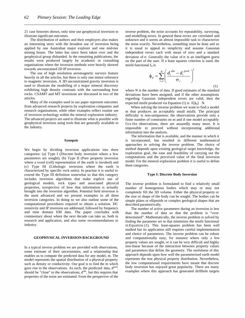
inverse problem, the noise accounts for repeatability, surveying, and modelling errors. In general these errors are correlated and unknown and it seems an almost impossible task to characterize the noise exactly. Nevertheless, something must be done and so it is usual to appeal to simplicity and assume Gaussian independent errors each with mean of zero and a standard deviation of s. Generally the value of s is an intelligent guess on the part of the user. If a least squares criterion is used, the misfit functional fd is

å=

÷÷ø

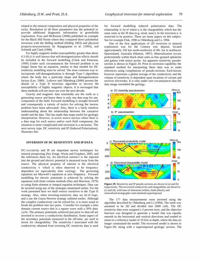
öççè

æ -=

N

i i

pred

i

obs

id

dd

1

2

sf

(1)

where N is the number of data. If good estimates of the standard deviations have been assigned, and if the other assumptions regarding Gaussian independent errors are valid, then the expected misfit produced via Equation (1) is E[fd] Ν .

When solving the inverse problem we want to find a model m that produces an acceptably small misfit. The principal difficulty is non-uniqueness: the observations provide only a finite number of constraints on m and if one model acceptably f i ts the observations, there are assuredly many more. It is impossible to proceed without incorporating additional information into the analysis.

The information that is available, and the manner in which it is incorporated, has resulted in different mathematical approaches to solving the inverse problem. The choice of method depends upon existing geological target knowledge, the exploration goal, the ease and feasibility of carrying out the computations and the perceived value of the final inversion model. For the mineral exploration problem it is useful to define three categories.

Type I: Discrete Body Inversion

The inverse problem is formulated to find a relatively small number of homogenous bodies which may or may not completely fill the 3D volume. Either the physical property or the size or shape of the body can be sought. The bodies can be simple plates or ellipsoids or complex geological shapes that are described parametrically.

The number of active parameters during an inversion is less than the number of data so that the problem is “over-determined”. Mathematically, the inverse problem is solved by finding the parameter set m that minimizes the misfit functional in Equation (1). This least-squares problem has been well studied but its application still requires careful implementation and choice of parameters. The inverse problem can be robust and computationally easy, for instance where only a few property values are sought, or it can be very difficult and highly non-linear because of the interaction between property values and parameters that define the geometry. The usefulness of this approach depends upon how well the parameterized earth model represents the true physical property distribution. Nevertheless, the low computational requirements have meant that discrete body inversion has enjoyed great popularity. There are many examples where this approach has generated drillhole targets

Plenary Session: The Leading Edge_________________________________________________________________________________________62

and provided important geological information. We present some in this paper.

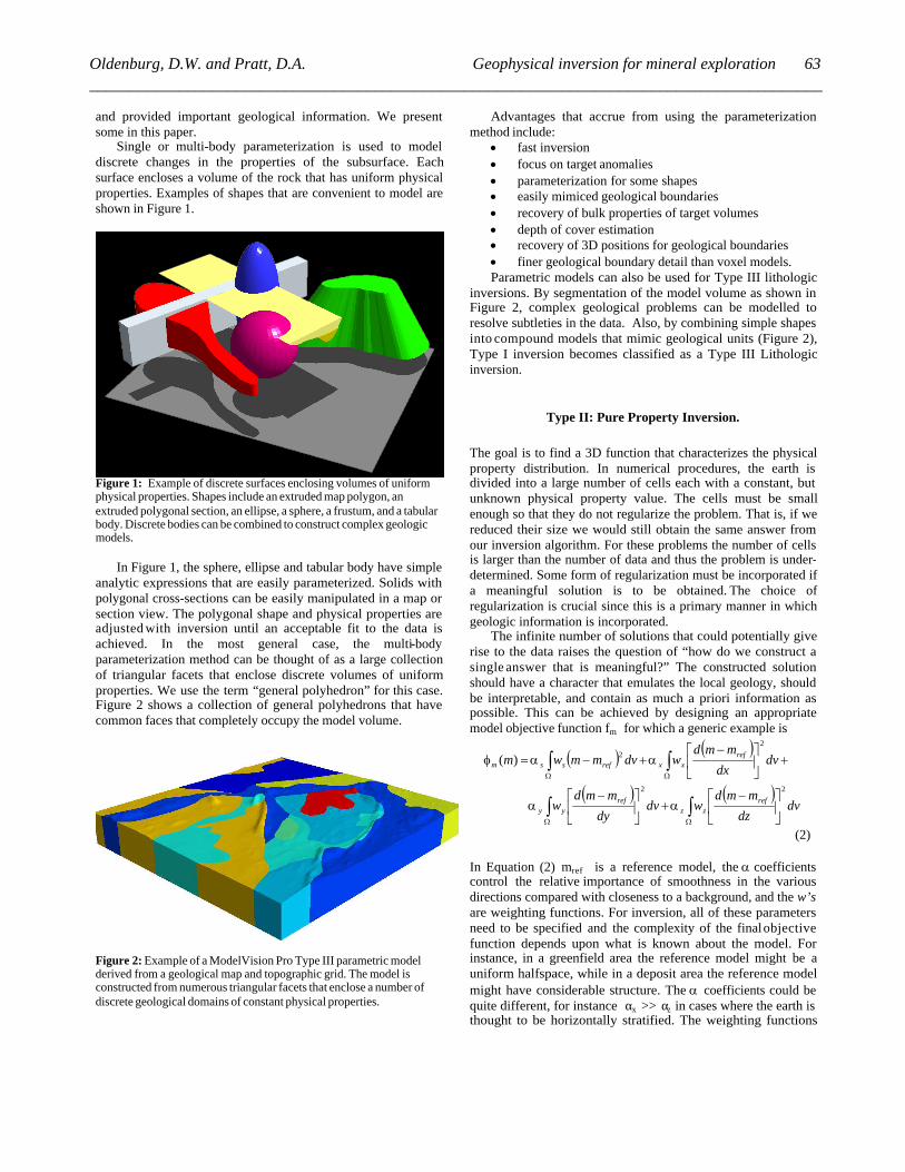
Single or multi-body parameterization is used to model discrete changes in the properties of the subsurface. Each surface encloses a volume of the rock that has uniform physical properties. Examples of shapes that are convenient to model are shown in Figure 1.

Figure 1: Example of discrete surfaces enclosing volumes of uniform physical properties. Shapes include an extruded map polygon, an extruded polygonal section, an ellipse, a sphere, a frustum, and a tabular body. Discrete bodies can be combined to construct complex geologic models.

In Figure 1, the sphere, ellipse and tabular body have simple analytic expressions that are easily parameterized. Solids with polygonal cross-sections can be easily manipulated in a map or section view. The polygonal shape and physical properties are adjusted with inversion until an acceptable fit to the data is achieved. In the most general case, the multi-body parameterization method can be thought of as a large collection of triangular facets that enclose discrete volumes of uniform properties. We use the term “general polyhedron” for this case. Figure 2 shows a collection of general polyhedrons that have common faces that completely occupy the model volume.

Figure 2: Example of a ModelVision Pro Type III parametric model derived from a geological map and topographic grid. The model is constructed from numerous triangular facets that enclose a number of discrete geological domains of constant physical properties.

Advantages that accrue from using the parameterization method include:

· fast inversion · focus on target anomalies · parameterization for some shapes · easily mimiced geological boundaries · recovery of bulk properties of target volumes · depth of cover estimation · recovery of 3D positions for geological boundaries · finer geological boundary detail than voxel models. Parametric models can also be used for Type III lithologic

inversions. By segmentation of the model volume as shown in Figure 2, complex geological problems can be modelled to resolve subtleties in the data. Also, by combining simple shapes into compound models that mimic geological units (Figure 2), Type I inversion becomes classified as a Type III Lithologic inversion.

Type II: Pure Property Inversion.

The goal is to find a 3D function that characterizes the physical property distribution. In numerical procedures, the earth is divided into a large number of cells each with a constant, but unknown physical property value. The cells must be small enough so that they do not regularize the problem. That is, if we reduced their size we would still obtain the same answer from our inversion algorithm. For these problems the number of cells is larger than the number of data and thus the problem is under-determined. Some form of regularization must be incorporated if a meaningful solution is to be obtained. The choice of regularization is crucial since this is a primary manner in which geologic information is incorporated.

The infinite number of solutions that could potentially give rise to the data raises the question of “how do we construct a single answer that is meaningful?” The constructed solution should have a character that emulates the local geology, should be interpretable, and contain as much a priori information as possible. This can be achieved by designing an appropriate model objective function fm for which a generic example is

( ) ( )

( ) ( )òò

òò

WW

WW

úû

ùêë

é -+ú

û

ùêë

é -

+úû

ùêë

é -+-=

dvdz

mmdwdv

dy

mmdw

dvdx

mmdwdvmmwm

ref

zz

ref

yy

ref

xxrefssm

22

2

2)(

aa

aaf

(2)

In Equation (2) mref is a reference model, the a coefficients control the relative importance of smoothness in the various directions compared with closeness to a background, and the w’s are weighting functions. For inversion, all of these parameters need to be specified and the complexity of the final objective function depends upon what is known about the model. For instance, in a greenfield area the reference model might be a uniform halfspace, while in a deposit area the reference model might have considerable structure. The a coefficients could be quite different, for instance αx >> αz in cases where the earth is thought to be horizontally stratified. The weighting functions

Oldenburg, D.W. and Pratt, D.A. Geophysical inversion for mineral exploration __________________________________________________________________________________________

63

can also be used to help honour prior information at various locations in the recovered model. The task of constructing a good model objective function is non-trivial. Nevertheless, it is a crucial part of the problem since the character and some of the structure observed in the final model will arise from the details about fm

The inverse problem is formulated as an optimization problem where we minimize

f(m)=fd(m)+bf

m(m)

(3)

In Equation (3) b is a trade-off parameter or Tikhonov parameter (Tikhonov and Arsenin, 1977) that is adjusted throughout the inversion so that, upon completion, a model with a desired misfit is achieved. To solve the problem numerically, the earth volume is divided into a number of cells each of which has a constant, but unknown, value of the physical property. The model objective function and forward modelling equations are discretized using the gridded earth volume and the total objective function to be minimized is

( ) ( ) 22

)()( refmobs

d mmWdmFWm -+-= bf

(4) where W dWm are matrices and F is the forward modelling operator. The objective function is differentiated to generate gradient equations which are subsequently solved. Numerous methodologies are possible but typically a Gauss-Newton procedure is implemented. The solution is achieved iteratively and at each iteration, a perturbation dm is found by solving

( ) )()()( mgmWWmJmJ m

T

mT -=+ db

(5) where J is the sensitivity whose elements are J ij = δdi/δmj and g(m) is the gradient. (See Nocedal and Wright 1999, or Boyd and Vandenberghe, 2004 for extensive background on numerical optimization).

The Gauss-Newton methodology is general and can be applied to different geophysical surveys to recover physical properties in one, two, and three dimensions. It can also form the numerical procedure for estimating parameters in Type I or Type III inversions.

Implementing the inversion procedure outlined above is straight-forward, but it requires care. First, the misfit objective functional needs to be chosen and thus an estimate of the standard deviation of each datum needs to be supplied. An important aspect is to assign the right relative error for various data. The unknown scaling factor controlling the overall magnitude can often be extracted from the inversion algorithm itself. Second, the model objective function must be specified and this requires assembling prior knowledge about the model. The third essential item pertains to the selection of the trade-off parameter. When Equation (3) is minimized for a specific b it produces a model that has a quantifiable misfit and model norm. The optimization can be carried out for many values of b t o

produce the Tikhonov, or trade-off, curve that is shown schematically in Figure 3.

Figure 3: A typical trade-off curve is shown, the dashed line indicates the desired misfit.

The Tikhonov curve typically has the shape of an "L". If the

data errors were properly estimated then the point on the curve that corresponds to ΦdN would be a good choice. However, if the data errors have not been properly estimated then some other point on the curve should be selected. On the left hand side of this curve, which corresponds to large β, it is possible to obtain a significant decrease in the misfit without greatly increasing the model norm. In this area of the curve we are fitting geophysical signal. The right hand portion of the curve shows that the model norm (i.e. structure) increases significantly with only a small decrease in misfit. In this realm we are fitting the noise. So we want to be somewhere near the kink of this curve. Automated methods, L-curve (Hanson, 1998) and GCV (Vogel, 2001), exist to find these solutions. Background about these items and other aspects of Type II inversions can be found in the tutorial paper by Oldenburg and Li, 2005.

The acceptance of Type II inversions has been tied to computing performance. In the early 1990s when this technology was emerging, large problems, characterized by a few thousand cells, were taking 12 hours to invert. Basically that meant only one or two runs per day. Since the inversion needed to be rerun a number of times, with modified error assignments and different objective functions, this was initially an impediment. However, as computational power increased, so did the acceptance of the technology.

There are three computational roadblocks for the inversion: (a) forward modelling; (b) calculation of a large sensitivity matrix; and (c) solving a large system of equations. However, as computer power progressed, it soon became possible to carry out inversions in 3D. If there are M model parameters to be solved, then the Gauss-Newton equations are of size M´M. Going from 2D to 3D results in a large increase in matrix size and hence computation time. An array of mathematical tools, like Conjugate Gradient solvers with effective pre-conditioners, and wavelet compression schemes to solve a reduced matrix (Li and


Oldenburg, 2003) played an important role in the technology transition.

Research in this area has concentrated upon: developing algorithms that can work with progressively larger problems, inverting more complicated data sets like frequency and time domain EM data, and modifying algorithms to incorporate physical and geologic constraints. Essentially these algorithms are transitioning towards carrying out Type III inversions.

Type III: Lithologic Inversion

The inverse problem is formulated in the geologic domain and the relationship between rock units and physical properties must be well understood. Each cell in the model has a particular rock type attached to it and the cells completely fill the volume. A “cell” could be a small rectangular unit as employed in a Type II problem, a larger discrete body as in Type I, or a combination of the two. Parameters can be location of boundaries and/or rock type. The problems can be over-determined or under-determined and solutions can be obtained either by deterministic or statistical procedures.

We note that the above classifications are mainly provided as a framework rather than a way to categorize different inversion algorithms. Many existing algorithms have the potential to be implemented in more than one category. For instance, VPmg (Fullagar 2004) can alter the location of an interface, or it can find a smooth distribution of properties within a defined geologic unit, so it has elements of both Type I and Type II inversions, and depending upon its implementation, can be considered to carry out a Type III inversion. Similarly, the existence of reference models and bound constraints can allow the UBC-GIF inversions to operate in a Type II or Type III mode. Also, ModelVision (Pratt et al. 2007) can be thought of as a hybrid that incorporates aspects of Type I and Type III methodologies. Other formulations, such as the geostatistical inversions in GeoModeller (Guillen et al. 2004) and stylized inversion in QuickMag (Pratt et al. 2001) are more directly formulated as a Type III inversion.

The important message is that all practitioners share a similar goal of trying to extract a geologically meaningful interpretation from the geophysical data. Since all require input of a priori information, invariably there will be similarities in functionality. Which procedure is adopted depends upon the geological domain, geological resolution, precision, labour cost, computation time and interactivity. The sizes of problems can vary from finding a few tens of parameters (a simple Type I problem) to finding millions of parameters (in a Type II or Type III problem). Computation times are commensurate with this and can vary from a few seconds to days.

Research on Type I inversions has focused on extending the use of simple model shapes to emulate complex geological model problems that are suited to the detailed investigation of mineral deposits. Type I algorithms are generally suited to interactive user-guided inversions of an anomaly complex, but not direct inversion of a complete survey (Pratt, Foss and Roberts, 2006). The Type I methods are excellent for mapping sharp contrasts in physical properties such as formation boundaries, dykes, folded volcanic units, diapirs and plutons.

The inversion is normally applied on a piece-wise basis by focussing on individual anomaly complexes.

Discrete Body and Voxel Model Comparison

Type II methods are well suited to inversion of continuous property changes associated with mineralization and alteration events and continuous mapping of physical properties over large areas. Before launching into examples of inversion we make a few comments about resolution in Type I and Type II parameterizations.

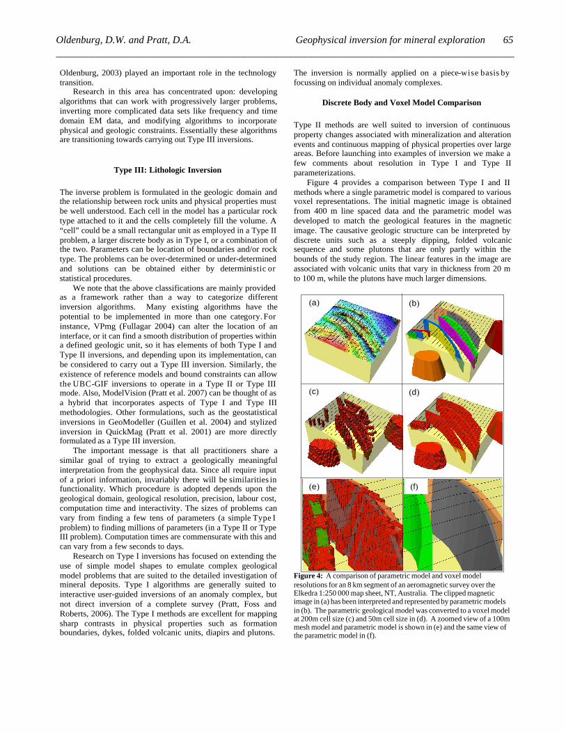
Figure 4 provides a comparison between Type I and II methods where a single parametric model is compared to various voxel representations. The initial magnetic image is obtained from 400 m line spaced data and the parametric model was developed to match the geological features in the magnetic image. The causative geologic structure can be interpreted by discrete units such as a steeply dipping, folded volcanic sequence and some plutons that are only partly within the bounds of the study region. The linear features in the image are associated with volcanic units that vary in thickness from 20 m to 100 m, while the plutons have much larger dimensions.

Figure 4: A comparison of parametric model and voxel model resolutions for an 8 km segment of an aeromagnetic survey over the Elkedra 1:250 000 map sheet, NT, Australia. The clipped magnetic image in (a) has been interpreted and represented by parametric models in (b). The parametric geological model was converted to a voxel model at 200m cell size (c) and 50m cell size in (d). A zoomed view of a 100m mesh model and parametric model is shown in (e) and the same view of the parametric model in (f).

(a) (b)

(c) (d)

(e) (f)


65

The image in Figure 4b can be thought of as a high resolution image of the earth. If the parameterization is correct, then this degree of resolution might represent reality. In effect, resolution has been imparted to the image via the parameterization. Type II inversions generally look more diffuse because there is no regularization imposed by the discretization of the volume; structure that is different from a background is a consequence of the data and geophysical data do not intrinsically possess high resolution. Nevertheless, to see how the primary geological features in a parametric model would appear if the earth were discretized with different cell sizes, we show the results of using 200, 100 and 50 m cells. At 200 m, much of the detail is lost and it is not until the mesh size is reduced to 50 m is there a reasonable representation of the geological detail.

At 200 m voxel size, the number of cells in the model is 115,500 and at 50 m the number of cells grows to 1,848,000 if a regular structured mesh is used. An adaptive mesh, say with VPmg, can provide better resolution at interfaces with fewer cells.

In this paper we attempt to provide examples of how these three types of inversion have been applied over the last decade. We detail our own developments in this field and draw on the work of others to illustrate the rich set of inversion options that are now available to assist in discovery and delineation of mineral deposits.

INVERSION OF POTENTIAL FIELD DATA

Inversion of potential field data has advanced rapidly over the last 10 years as explorers attempt to extract more value from their surveys. The outstanding breakthrough in airborne gravity gradiometry at the mid-point of the decade has also been a strong catalyst for developing large scale inversions of this new generation of survey. The aeromagnetic method, however is still the most widely used geophysical survey for mineral exploration as it provides economical, high resolution and deep investigation of large areas. When outcrop is sparse and drilling is limited, the aeromagnetic image is the surrogate geological map. It is however, becoming more frequent for potential field data to be inverted. In the following discourse we provide practical examples of how the three inversion types have been used for different styles of the exploration problem.

Type I: Discrete Body Inversion

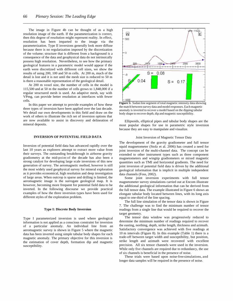
Type I parameterized inversion is used where geological information is not applied as a conscious constraint for inversion of a particular anomaly. An individual line from an aeromagnetic survey is shown in Figure 5 where the magnetic data has been inverted using simple tabular body shapes for each magnetic anomaly. The primary objective for this inversion is the estimation of cover depth, formation dip and magnetic susceptibility.

Figure 5: Sudan line segment of total magnetic intensity data showing the match between survey data and model responses. Each magnetic anomaly is inverted to recover a model based on the dipping tabular body shape to recover depth, dip and magnetic susceptibility.

Ellipsoids, elliptical pipes and tabular body shapes are the most popular shapes for use in parametric style inversion because they are easy to manipulate and visualize.

Joint Inversion of Magnetic Tensor Data

The development of the gravity gradiometer and full tensor squid magnetometer (Stolz et al. 2006) has created a need for joint inversion of the multi-channel data. The concept can be extended to other instrument types such as three component magnetometers and wingtip gradiometers or mixed magnetic quantities such as TMI and horizontal gradients. The need for joint inversion of potential field data is driven by the additional geological information that is implicit in multiple independent data channels (Foss, 2002).

Some joint inversion experiments with full tensor magnetometer survey simulations carried out at Encom illustrate the additional geological information that can be derived from the full tensor data. The example illustrated in Figure 6 shows an elongate tabular body located between lines, with its long axis equal to one-third of the line spacing.

The full line simulation of the tensor data is shown in Figure 7. The challenge was to find the minimum number of tensor readings from a single line that would be required to recover the target geometry.

The tensor data window was progressively reduced to determine the minimum number of readings required to recover the easting, northing, depth, strike length, thickness and azimuth. Satisfactory convergence was achieved with five readings at 10 m intervals (Figure 8). In this example (Table 1) there is a trade-off between target width and susceptibility, but position, strike length and azimuth were recovered with excellent precision. All six tensor channels were used in the inversion. While only five channels are required due to redundancy, the use of six channels is beneficial in the presence of noise.

These trials were based upon noise-free simulations, and longer data samples will be required in the presence of noise.


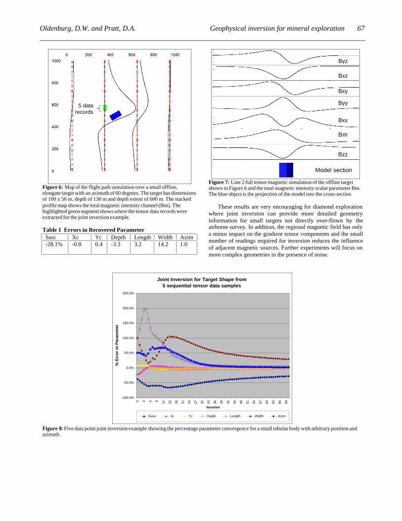
Figure 6: Map of the flight path simulation over a small offline, elongate target with an azimuth of 60 degrees. The target has dimensions of 100 x 50 m, depth of 130 m and depth extent of 600 m. The stacked profile map shows the total magnetic intensity channel (Bm). The highlighted green segment shows where the tensor data records were extracted for the joint inversion example.

Table 1 Errors in Recovered Parameter Susc Xc Yc Depth Length Width Azim -28.1% -0.8 0.4 -3.3 3.2 14.2 1.0

Figure 7: Line 2 full tensor magnetic simulation of the offline target shown in Figure 6 and the total magnetic intensity scalar parameter Bm. The blue object is the projection of the model into the cross-section

These results are very encouraging for diamond exploration

where joint inversion can provide more detailed geometry information for small targets not directly over-flown by the airborne survey. In addition, the regional magnetic field has only a minor impact on the gradient tensor components and the small number of readings required for inversion reduces the influence of adjacent magnetic sources. Further experiments will focus on more complex geometries in the presence of noise.

Joint Inversion for Target Shape from

5 sequential tensor data samples

-100.0%

-50.0%

0.0%

50.0%

100.0%

150.0%

200.0%

250.0%

0 3 6 9

12

15

18

21

24

27

30

33

36

39

42

45

48

51

54

57

60

63

66

69

Iteration

% E

rro

r in

Pa

ram

ete

r

Susc Xc Yc Depth Length Width Azim

Figure 8: Five data point joint inversion example showing the percentage parameter convergence for a small tabular body with arbitrary position and azimuth.

Byz

Bxz

Bxy

Byy

Bxx

Bm

Bzz

Model section

5 data records


67

Type II: Pure Property Inversion

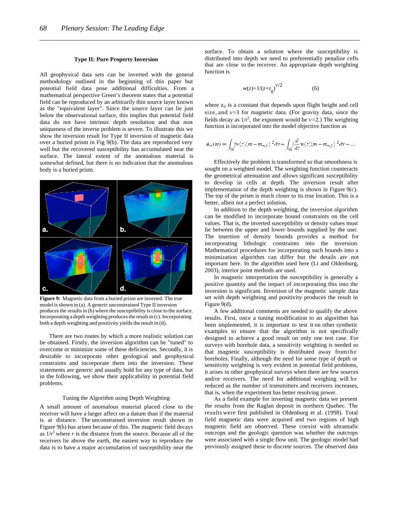
All geophysical data sets can be inverted with the general methodology outlined in the beginning of this paper but potential field data pose additional difficulties. From a mathematical perspective Green’s theorem states that a potential field can be reproduced by an arbitrarily thin source layer known as the "equivalent layer". Since the source layer can lie just below the observational surface, this implies that potential field data do not have intrinsic depth resolution and that non-uniqueness of the inverse problem is severe. To illustrate this we show the inversion result for Type II inversion of magnetic data over a buried prism in Fig 9(b). The data are reproduced very well but the recovered susceptibility has accumulated near the surface. The lateral extent of the anomalous material is somewhat defined, but there is no indication that the anomalous body is a buried prism.

Figure 9: Magnetic data from a buried prism are inverted. The true model is shown in (a). A generic unconstrained Type II inversion produces the results in (b) where the susceptibility is close to the surface. Incorporating a depth weighting produces the result in (c). Incorporating both a depth weighting and positivity yields the result in (d).

There are two routes by which a more realistic solution can be obtained. Firstly, the inversion algorithm can be "tuned" to overcome or minimize some of these deficiencies. Secondly, it is desirable to incorporate other geological and geophysical constraints and incorporate them into the inversion. These statements are generic and usually hold for any type of data, but in the following, we show their applicability in potential field problems.

Tuning the Algorithm using Depth Weighting

A small amount of anomalous material placed close to the receiver will have a larger affect on a datum than if the material is at distance. The unconstrained inversion result shown in Figure 9(b) has arisen because of this. The magnetic field decays as 1/r3 where r is the distance from the source. Because all of the receivers lie above the earth, the easiest way to reproduce the data is to have a major accumulation of susceptibility near the

surface. To obtain a solution where the susceptibility is distributed into depth we need to preferentially penalize cells that are close to the receiver. An appropriate depth weighting function is

w(z)=1/(z+z0)n/2

(6)

where z0 is a constant that depends upon flight height and cell size, and n=3 for magnetic data. (For gravity data, since the fields decay as 1/r2, the exponent would be n=2.) The weighting function is incorporated into the model objective function as

Effectively the problem is transformed so that smoothness is sought on a weighted model. The weighting function counteracts the geometrical attenuation and allows significant susceptibility to develop in cells at depth. The inversion result after implementation of the depth weighting is shown in Figure 9(c). The top of the prism is much closer to its true location. This is a better, albeit not a perfect solution.

In addition to the depth weighting, the inversion algorithm can be modified to incorporate bound constraints on the cell values. That is, the inverted susceptibility or density values must lie between the upper and lower bounds supplied by the user. The insertion of density bounds provides a method for incorporating lithologic constraints into the inversion. Mathematical procedures for incorporating such bounds into a minimization algorithm can differ but the details are not important here. In the algorithm used here (Li and Oldenburg, 2003), interior point methods are used.

In magnetic interpretation the susceptibility is generally a positive quantity and the impact of incorporating this into the inversion is significant. Inversion of the magnetic sample data set with depth weighting and positivity produces the result in Figure 9(d).

A few additional comments are needed to qualify the above results. First, once a tuning modification to an algorithm has been implemented, it is important to test it on other synthetic examples to ensure that the algorithm is not specifically designed to achieve a good result on only one test case. For surveys with borehole data, a sensitivity weighting is needed so that magnetic susceptibility is distributed away from the boreholes. Finally, although the need for some type of depth or sensitivity weighting is very evident in potential field problems, it arises in other geophysical surveys when there are few sources and/or receivers. The need for additional weighing will be reduced as the number of transmitters and receivers increases, that is, when the experiment has better resolving power.

As a field example for inverting magnetic data we present the results from the Raglan deposit in northern Quebec. The results were first published in Oldenburg et al. (1998). Total field magnetic data were acquired and two regions of high magnetic field are observed. These coexist with ultramafic outcrops and the geologic question was whether the outcrops were associated with a single flow unit. The geologic model had previously assigned these to discrete sources. The observed data


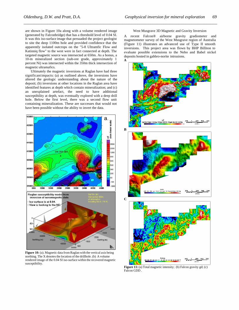
are shown in Figure 10a along with a volume rendered image (generated by Falconbridge) that has a threshold level of 0.04 SI. It was this iso-surface image that persuaded the project geologist to site the deep 1100m hole and provided confidence that the apparently isolated outcrops on the "5-8 Ultramfic Flow and Katinniq flow" to the west were in fact connected at depth. The targeted magnetic source was intersected at 650m. As a bonus, a 10-m mineralized section (sub-ore grade, approximately 1 percent Ni) was intersected within the 350m thick intersection of magnetic ultramafics.

Ultimately the magnetic inversions at Raglan have had three significant impacts: (a) as outlined above, the inversions have altered the geologic understanding about the nature of the deposit; (b) inversions at other locations in the Raglan area have identified features at depth which contain mineralization; and (c) an unexplained artefact, the need to have additional susceptibility at depth, was eventually explored with a deep drill hole. Below the first level, there was a second flow unit containing mineralization. These are successes that would not have been possible without the ability to invert the data.

Figure 10: (a). Magnetic data from Raglan with the vertical axis being northing. The X denotes the location of the drillhole. (b) A volume rendered image of the 0.04 SI iso-surface within the recovered magnetic susceptibility.

West Musgrave 3D Magnetic and Gravity Inversion

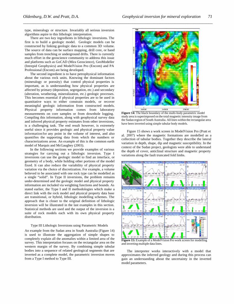
A recent Falcon® airborne gravity gradiometer and magnetometer survey of the West Musgrave region of Australia (Figure 11) illustrates an advanced use of Type II smooth inversions. This project area was flown by BHP Billiton to evaluate possible extensions to the Nebo and Babel nickel deposits hosted in gabbro-norite intrusions. A

B

C

Figure 11: (a) Total magnetic intensity; (b) Falcon gravity gd; (c) Falcon GDD .


69

While not disclosing specifics of their inversion methodologies, BHP Billiton does invert the Falcon data directly from the line data and allows the inversion process to minimise the noise that is inherent in the system. Figure 12 shows an example inversion of the gravity data in a region around the known deposits.

The method was then applied to the complete survey area in Figure 11 using both the Falcon® gravity gradiometer and magnetic data inversions. The anomalous density and magnetic susceptibility were used to define potential petrophysical property classes as illustrated in Figure 13. By clustering the joint density and susceptibility values, (Figure 13) they are able to isolate anomalous regions that might otherwise be missed by manual analysis of the volumes. A

B

Figure 12: (a) area of detailed gravity gradient (GDD) data covering the Nebo and Babel deposits (b) The clustered density distributions derived from 3D smooth inversion. Blue clusters are high density and brown clusters are low density.

This work parallels that by Phillips (2002) where regional gravity and magnetic data over the San Nicolas area were inverted individually and volumes that exhibited high density and susceptibility were isolated. Of the five regions identified, one was the San Nicolas deposit, two were areas of known mineralization, and one unit was a known non-mineralized geologic unit. A

B

Figure 13: (a) This cluster diagram was used to isolate specific density and magnetic susceptibility regions. Clustered density and magnetic susceptibility distributions are mapped across the complete survey (b) Only the most anomalous density and magnetic susceptibility values are displayed in the image where pink = high density and orange = high susceptibility.

Type III: Lithologic Inversions

Generic inversions can be of value but the non-uniqueness can be reduced by incorporating constraints on the physical properties and other geophysical and geologic information. Moreover, geologic answers are best formulated in terms of rock


type, mineralogy or structure. Invariably all serious inversion algorithms aspire to this lithologic interpretation.

There are two key ingredients in lithologic inversions. The first is to build a geologic model. Geologic models can be constructed by linking geologic data to a common 3D volume. The source of data can be surface mapping, drill core, or hand samples from trenching or underground drifts. There is currently much effort in the geoscience community to address this issue and platforms such as GoCAD (Mira Geoscience), GeoModeller (Intrepid Geophysics) and ModelVision Pro (Encom) and PA Professional (Encom) are being developed.

The second ingredient is to have petrophysical information about the various rock units. Knowing the dominant factors (mineralogy or porosity) that control physical properties is important, as is understanding how physical properties are affected by primary (deposition, segregation, etc.) and secondary (alteration, weathering, mineralization, etc.) geologic processes. This becomes essential if physical properties are to be used in quantitative ways to either constrain models, or recover meaningful geologic information from constructed models. Physical property information comes from laboratory measurements on core samples or from downhole logging. Compiling this information, along with geophysical survey data and inferred physical property estimates from other inversions, is a challenging task. The end result however, is extremely useful since it provides geologic and physical property value information for any point in the volume of interest, and also quantifies the supporting data from which the numbers or characterizations arose. An example of this is the common earth model of Marquis and McGaughey (2003).

In the following sections we provide examples of various strategies for carrying out a lithologic inversion. Type I inversions can use the geologic model to find an interface, or geometry of a body, while holding other portions of the model fixed. It can also reduce the variability of physical property variation via the choice of discretization. For example, a volume believed to be associated with one rock type can be modelled as a single “solid”. In Type II inversions, the problem remains under-determined and the geologic model and physical property information are included via weighting functions and bounds. As stated earlier, the Type I and II methodologies which make a direct link with the rock model and physical property data base are transitional, or hybrid, lithologic modelling schemes. The approach that is closer to the original definition of lithologic inversion will be illustrated in the last examples in this section. Statistical methods are used and the output of the inversion is a suite of rock models each with its own physical property distribution.

Type III Lithologic Inversions using Parametric Models

An example from the Sudan area in South Australia (Figure 14) is used to illustrate the aggregation of simple shapes to completely explain all the anomalies within a limited area of the survey. This interpretation focuses on the rectangular area on the western margin of the survey. By combining simple tabular bodies into a sequence of related geological segments that are inverted as a complete model, the parametric inversion moves from a Type I method to Type III.

Figure 14: The black boundary of the multi-body parametric model study area is superimposed on the total magnetic intensity image from the Sudan region of South Australia. All lines within the rectangular area have been inverted using simple tabular body models.

Figure 15 shows a work screen in ModelVision Pro (Pratt et al. 2007) where the magnetic formations are modelled as a collection of tabular bodies. Together they describe the lateral variation in depth, shape, dip and magnetic susceptibility. In the context of the Sudan project, geologists were able to understand the depth of cover, anticlinal structure and magnetic property variations along the fault truncated fold limbs.

Figure 15: Example of a ModelVision Pro work screen for modelling and inverting multiple data lines.

The interpreter works interactively with a model that approximates the inferred geology and during this process can gain an understanding about the uncertainty in the inverted model parameters.


71

Type III Stylized 3D Inversion

Pratt et al. (2001) introduced stylized inversion as a method for direct interpretation of discrete magnetic anomalies. The method provides the user with the controls for rapid testing of different geological styles for a given target anomaly without the need for manual construction of the model. In this context a geological style refers to the shape of the geological model and distribution of physical properties. The concept was designed to provide the user with rapid feedback on geological questions while interpreting a magnetic survey.

The stylized method uses regularized inversion with a trade-off between the quality of the data mismatch and the quality of the geological model style. This principle is illustrated in Figure 3 except the horizontal axis is the quality of the geological match and the vertical axis is the quality of the data match. The objective is to locate the solution that provides the best data match with the best geological match. The solution occurs at the corner of the L -type curve. The interpreter is able to test different plausible geological styles for each given magnetic anomaly.

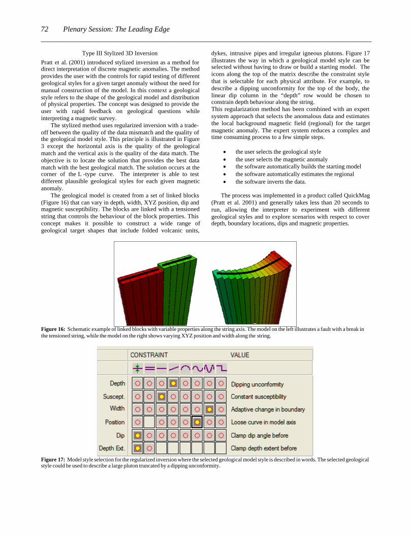
The geological model is created from a set of linked blocks (Figure 16) that can vary in depth, width, XYZ position, dip and magnetic susceptibility. The blocks are linked with a tensioned string that controls the behaviour of the block properties. This concept makes it possible to construct a wide range of geological target shapes that include folded volcanic units,

dykes, intrusive pipes and irregular igneous plutons. Figure 17 illustrates the way in which a geological model style can be selected without having to draw or build a starting model. The icons along the top of the matrix describe the constraint style that is selectable for each physical attribute. For example, to describe a dipping unconformity for the top of the body, the linear dip column in the “depth” row would be chosen to constrain depth behaviour along the string. This regularization method has been combined with an expert system approach that selects the anomalous data and estimates the local background magnetic field (regional) for the target magnetic anomaly. The expert system reduces a complex and time consuming process to a few simple steps.

· the user selects the geological style · the user selects the magnetic anomaly · the software automatically builds the starting model · the software automatically estimates the regional · the software inverts the data.

The process was implemented in a product called QuickMag

(Pratt et al. 2001) and generally takes less than 20 seconds to run, allowing the interpreter to experiment with different geological styles and to explore scenarios with respect to cover depth, boundary locations, dips and magnetic properties.

Figure 16: Schematic example of linked blocks with variable properties along the string axis. The model on the left illustrates a fault with a break in the tensioned string, while the model on the right shows varying XYZ position and width along the string.

Figure 17: Model style selection for the regularized inversion where the selected geological model style is described in words. The selected geological style could be used to describe a large pluton truncated by a dipping unconformity.


Stylized Inversion Example for San Nicolas

San Nicolas is a Cu-Zn massive sulphide deposit located in central Mexico in the state of Zacatecas. The deposit is a continuous, but geometrically complex, body of sulphides which is covered by 175-250 m of variable composition overburden. The local geology is also complex and contains numerous sedimentary and volcanic units. Numerous geophysical surveys have been carried out over the deposit and extensive drilling has been completed. As such, San Nicolas makes a good geophysical test site. We make use of it here and in a number of other locations in this paper.

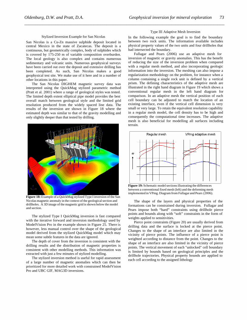
The San Nicolas DIGHEM magnetic survey data was interpreted using the QuickMag stylized parametric method (Pratt et al. 2001) where a range of geological styles was tested. The limited depth extent elliptical pipe model provides the best overall match between geological style and the limited grid resolution produced from the widely spaced line data. The results of the inversion are shown in Figure 18 where the estimated depth was similar to that of the gravity modelling and only slightly deeper than that tested by drilling.

Figure 18: Example of a QuickMag stylized Type I inversion of the San Nicolas magnetic anomaly in the context of the geological section and drillholes. A 3D image of the magnetic grid is shown below the model and section.

The stylized Type I QuickMag inversion is fast compared with the iterative forward and inversion methodology used by ModelVision Pro in the example shown in Figure 25. There is however, less manual control over the shape of the geological model derived from the stylized QuickMag model which may mean some subtle features in the data are ignored.

The depth of cover from the inversion is consistent with the drilling results and the distribution of magnetic properties is consistent with other modelling methods. This information was extracted with just a few minutes of stylized modelling.

The stylized inversion method is useful for rapid assessment of a large number of magnetic anomalies which can then be prioritized for more detailed work with constrained ModelVision Pro and UBC GIF, MAG3D inversions.

Type III Adaptive Mesh Inversion

In the following example the goal is to find the boundary between two rock units. The information available includes physical property values of the two units and four drillholes that had intersected the boundary.

Fullagar and Pears (2006) use an adaptive mesh for inversion of magnetic or gravity anomalies. This has the benefit of reducing the size of the inversion problem when compared with a regular mesh method, and also incorporating geologic information into the inversion. The meshing can also impose a regularization methodology on the problem, for instance when a column containing a single rock unit is defined by a vertical prism. The defining characteristics of the adaptive mesh are illustrated in the right hand diagram in Figure 19 which shows a conventional regular mesh in the left hand diagram for comparison. In an adaptive mesh the vertical position of each cell boundary can be adjusted to match the location of an existing interface, even if the vertical cell dimension is very small or very large. To retain the equivalent resolution capability in a regular mesh model, the cell density has to be high and consequently the computational time increases. The adaptive mesh is also beneficial for modelling all surfaces including terrain.

Figure 19: Schematic model sections illustrating the differences between a conventional fixed mesh (left) and the deforming mesh implemented in VPmg. Diagram from Fullagar and Pears (2006).

The shape of the layers and physical properties of the formations can be constrained during inversion. Fullagar and Pears impose both “hard” constraints using drillhole pierce points and bounds along with “soft” constraints in the form of weights applied to sensitivities.

Pierce point constraints (Figure 20) are usually derived from drilling data and the surface is locked at the pierce point. Changes to the shape of an interface are also limited in the vicinity of pierce points. The influence of a pierce point is weighted according to distance from the point. Changes to the shape of an interface are also limited in the vicinity of pierce points. The vertical movement of each "unlocked" cell boundary is limited by bounds based on geological principles and the drillhole trajectories. Physical property bounds are applied to each cell according to the assigned lithology


73

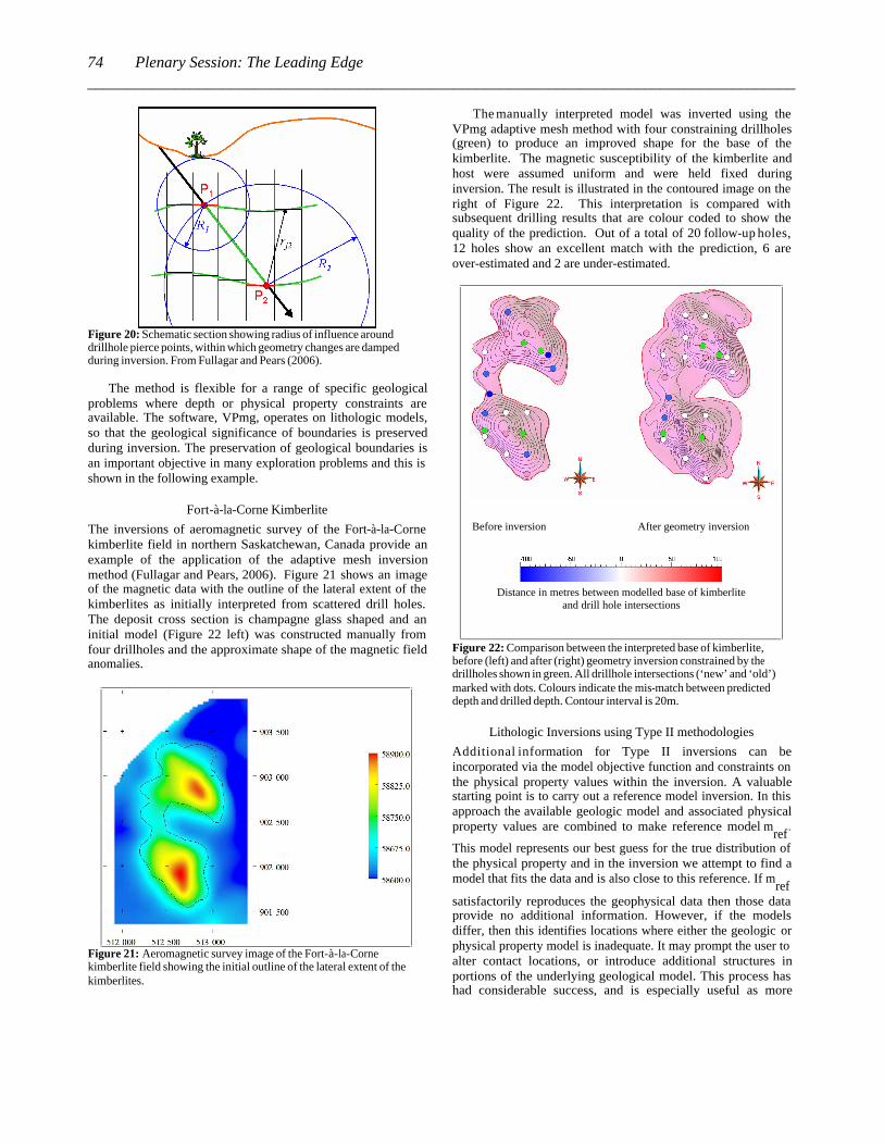
Figure 20: Schematic section showing radius of influence around drillhole pierce points, within which geometry changes are damped during inversion. From Fullagar and Pears (2006).

The method is flexible for a range of specific geological

problems where depth or physical property constraints are available. The software, VPmg, operates on lithologic models, so that the geological significance of boundaries is preserved during inversion. The preservation of geological boundaries is an important objective in many exploration problems and this is shown in the following example.

Fort-à-la-Corne Kimberlite

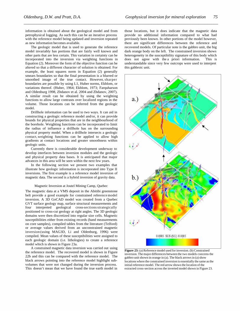
The inversions of aeromagnetic survey of the Fort-à-la-Corne kimberlite field in northern Saskatchewan, Canada provide an example of the application of the adaptive mesh inversion method (Fullagar and Pears, 2006). Figure 21 shows an image of the magnetic data with the outline of the lateral extent of the kimberlites as initially interpreted from scattered drill holes. The deposit cross section is champagne glass shaped and an initial model (Figure 22 left) was constructed manually from four drillholes and the approximate shape of the magnetic field anomalies.

Figure 21: Aeromagnetic survey image of the Fort-à-la-Corne kimberlite field showing the initial outline of the lateral extent of the kimberlites.

The manually interpreted model was inverted using the VPmg adaptive mesh method with four constraining drillholes (green) to produce an improved shape for the base of the kimberlite. The magnetic susceptibility of the kimberlite and host were assumed uniform and were held fixed during inversion. The result is illustrated in the contoured image on the right of Figure 22. This interpretation is compared with subsequent drilling results that are colour coded to show the quality of the prediction. Out of a total of 20 follow-up holes, 12 holes show an excellent match with the prediction, 6 are over-estimated and 2 are under-estimated.

Before inversion After geometry inversion

Distance in metres between modelled base of kimberlite and drill hole intersections

Figure 22: Comparison between the interpreted base of kimberlite, before (left) and after (right) geometry inversion constrained by the drillholes shown in green. All drillhole intersections (‘new’ and ‘old’) marked with dots. Colours indicate the mis-match between predicted depth and drilled depth. Contour interval is 20m.

Lithologic Inversions using Type II methodologies

Additional information for Type II inversions can be incorporated via the model objective function and constraints on the physical property values within the inversion. A valuable starting point is to carry out a reference model inversion. In this approach the available geologic model and associated physical property values are combined to make reference model m

ref.

This model represents our best guess for the true distribution of the physical property and in the inversion we attempt to find a model that fits the data and is also close to this reference. If m

ref

satisfactorily reproduces the geophysical data then those data provide no additional information. However, if the models differ, then this identifies locations where either the geologic or physical property model is inadequate. It may prompt the user to alter contact locations, or introduce additional structures in portions of the underlying geological model. This process has had considerable success, and is especially useful as more


information is obtained about the geological model and from petrophysical logging. As such this can be an iterative process with the reference model being updated and inversion repeated as new information becomes available.

The geologic model that is used to generate the reference model invariably has portions that are fairly well known and other parts that are less certain. This variation in certainty can be incorporated into the inversion via weighting functions in Equation (2). Moreover the form of the objective function can be altered so that a different character of solution is obtained. For example, the least squares norm in Equation (2) generally smears boundaries so that the final presentation is a blurred or smoothed image of the true contact. However, sharper boundaries are possible by using L1, Huber norms, Ekblom, or variations thereof. (Huber, 1964; Ekblom, 1973; Farquharson and Oldenburg 1998, Zhdanov et al. 2004 and Zhdanov, 2007). A similar result can be obtained by using the weighting functions to allow large contrasts over localized regions in the volume. Those locations can be inferred from the geologic model.

Drillhole information can be used to two ways. It can aid in constructing a geologic reference model and/or, it can provide bounds for physical properties that are in the neighbourhood of the borehole. Weighting functions can be incorporated to limit the radius of influence a drillhole has on the surrounding physical property model. When a drillhole intersects a geologic contact, weighting functions can be applied to allow high gradients at contact locations and greater smoothness within geologic units.

Currently there is considerable development underway to develop interfaces between inversion modules and the geologic and physical property data bases. It is anticipated that major advances in this area will be seen within the next few years.

In the following section we present two examples that illustrate how geologic information is incorporated into Type II inversions. The first example is a reference model inversion of magnetic data. The second is a hybrid inversion of gravity data.

Magnetic Inversion at Joutel Mining Camp, Quebec

The magnetic data at a VMS deposit in the Abitibi greenstone belt provide a good example for constrained reference model inversion. A 3D GoCAD model was created from a Quebec GVT surface geology map, surface structural measurements and four interpreted geological cross-sections strategically positioned to cross-cut geology at right angles. The 3D geologic domains were then discretized into regular size cells. Magnetic susceptibilities either from existing records (hand measurements on core samples), compiled tables from the literature (Telford) or average values derived from an unconstrained magnetic inversion (using MAG3D, Li and Oldenburg, 1996) were compiled. Mean values of these susceptibilities were assigned to each geologic domain (i.e. lithologies) to create a reference model which is shown in Figure 23a.

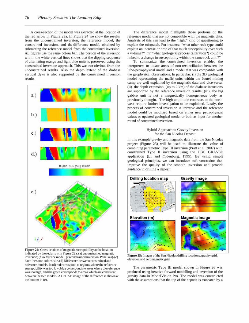
A constrained magnetic data inversion was carried out using the reference model. The recovered model is shown in Figure 22b and this can be compared with the reference model. The black arrows pointing into the reference model highlight sub-volumes that were not changed during the inversion process. This doesn’t mean that we have found the true earth model in

those locations, but it does indicate that the magnetic data provide no additional information compared to what had previously been known. In other portions of the model however, there are significant differences between the reference and recovered models. Of particular note is the gabbro unit, the big dark orange body on the left. The constrained inversion shows heterogeneity in the susceptibility signature of this body which does not agree with the a priori information. This is understandable since very few outcrops were used to interpret this gabbroic unit.

Figure 23: (a) Reference model used for inversion. (b) Constrained inversion. The major differences between the two models concerns the gabbro unit shown in orange in (a). The black arrows in (a) show locations where the constrained inversion is essentially the same as the initial reference model. The red arrow shows the location of the extracted cross-section across the inverted model shown in Figure 23.


75

A cross-section of the model was extracted at the location of the red arrow in Figure 23a. In Figure 24 we show the results from the unconstrained inversion, the reference model, the constrained inversion, and the difference model, obtained by subtracting the reference model from the constrained inversion. All figures use the same colour bar. The portion of the inversion within the white vertical lines shows that the dipping sequence of alternating orange and light blue units is preserved using the constrained inversion approach. This was not obvious from the unconstrained results. Also the depth extent of the diabase vertical dyke is also supported by the constrained inversion results

Figure 24: Cross-sections of magnetic susceptibility at the location indicated by the red arrow in Figure 22a. (a) unconstrained magnetic inversion; (b) reference model; (c) constrained inversion. Panels (a)-(c) have the same color scale. (d) Difference between constrained and reference models. In (d) red correspond to regions where the reference susceptibility was too low, blue corresponds to areas where the reference was too high, and the green corresponds to areas which are consistent between the two models. A GoCAD image of the difference is shown at the bottom in (e).

The difference model highlights those portions of the reference model that are not compatible with the magnetic data. Analysis of this can lead to the “right” kind of questioning to explain the mismatch. For instance, “what other rock type could explain an increase or drop of that much susceptibility over such a volume?” Or “what geological process (alteration?) could be linked to a change in susceptibility within the same rock unit ?”

To summarize, the constrained inversion enabled the interpreters to locate areas of non-reconciliation between the litho-petrophysical model and a model that was compatible with the geophysical observations. In particular: (i) the 3D geological model representing the mafic units within the Joutel mining camp are well explained by the magnetic data and vice-versa; (ii) the depth extension (up to 2 km) of the diabase intrusions are supported by the reference inversion results; (iii) the big gabbro unit is not a magnetically homogeneous body as previously thought. The high amplitude contrasts to the north west require further investigation to be explained. Lastly, the process of constrained inversion is iterative and the reference model could be modified based on either new petrophysical values or updated geological model or both as input for another round of constrained inversion.

Hybrid Approach to Gravity Inversion for the San Nicolas Deposit

In this example gravity and magnetic data from the San Nicolas project (Figure 25) will be used to illustrate the value of combining parametric Type III inversion (Pratt et al. 2007) with constrained Type II inversion using the UBC GRAV3D application (Li and Oldenburg, 1995). By using simple geological principles, we can introduce soft constraints that improve the quality of the smooth inversion and provide guidance in drilling a deposit.

Figure 25: Images of the San Nicolas drilling locations, gravity grid, elevation and aeromagnetic grid.

The parametric Type III model shown in Figure 26 was produced using iterative forward modelling and inversion of the gravity data in ModelVision Pro. The model was constructed with the assumptions that the top of the deposit is truncated by a


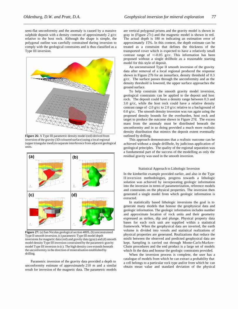
semi-flat unconformity and the anomaly is caused by a massive sulphide deposit with a density contrast of approximately 2 g/cc relative to the host rock. Although the shape is simple, the polygonal outline was carefully constrained during inversion to comply with the geological constraints and is thus classified as a Type III inversion.

Figure 26: A Type III parametric density model (red) derived from inversion of the gravity (3D coloured surface) using a local regional (upper triangular mesh) to separate interference from adjacent geological units.

Figure 27: (a) San Nicolas geological section 400S, (b) unconstrained Type II smooth inversion, (c) parametric Type III model depth inversions for magnetic data (red) and gravity data (gray) and (d) smooth model density Type III inversion constrained by the parametric gravity model Type III inversion in (c). The high density core extends beneath the unconformity in the direction of mineralisation established by drilling.

Parametric inversion of the gravity data provided a depth to

unconformity estimate of approximately 210 m and a similar result for inversion of the magnetic data. The parametric models

are vertical polygonal prisms and the gravity model is shown in gray in (Figure 27c) and the magnetic model is shown in red. The actual depth is 180 m indicating an estimation error of approximately 15%. In this context, the depth estimate can be treated as a constraint that defines the thickness of the transported cover which is expected to have a relatively small contrast range of +/-0.05 g/cc. This information has been proposed without a single drillhole as a reasonable starting model for this style of deposit.

An unconstrained Type II smooth inversion of the gravity data after removal of a local regional produced the response shown in Figure 27b for an isosurface, density threshold of 0.3 g/cc. The surface passes through the unconformity and as the density threshold is lowered, the upper surface approaches the ground surface.

To help constrain the smooth gravity model inversion, geological constraints can be applied to the deposit and host rock. The deposit could have a density range between 0.3 and 3.0 g/cc, while the host rock could have a relative density contrast range of -2.0 g/cc to 2.0 g/cc relative to a background of 0.0 g/cc. The smooth density inversion was run again using the proposed density bounds for the overburden, host rock and target to produce the outcome shown in Figure 27d. The excess mass from the anomaly must be distributed beneath the unconformity and in so doing provided a much more realistic density distribution that mimics the deposit extent eventually outlined by drilling.

This approach demonstrates that a realistic outcome can be achieved without a single drillhole, by judicious application of geological principles. The quality of the regional separation was a fundamental part of the success of the modelling as only the residual gravity was used in the smooth inversion.

Statistical Approach to Lithologic Inversion

In the kimberlite example provided earlier, and also in the Type II inversion methodologies, progress towards a lithologic solution was achieved by incorporating geologic information into the inversion in terms of parameterization, reference models and constraints on the physical properties. The inversion then generated a single model from which geologic information is extracted.

In statistically based lithologic inversions the goal is to generate many models that honour the geophysical data and geologic information. The geologic information includes number and approximate location of rock units and their geometry expressed as strikes, dip and plunge. Physical property data bases for each rock unit are supplied within a statistical framework. When the geophysical data are inverted, the earth volume is divided into voxels and statistical realizations of physical properties are generated. Realizations that reduce the misfit between the observed and predicted geophysical data are kept. Sampling is carried out through Monte-Carlo Markov-Chain procedures and the end product is a large set of models which fit the data and honour the geologic constraints provided.

When the inversion process is complete, the user has a catalogue of models from which he can extract a probability that a cell belongs to a particular rock type and/or from which he can obtain mean value and standard deviation of the physical


77

property of the cell. (For example, see Bosch, 1999, Bosch and McGaughey, 2001, Guillen et al, 2004 and Lane, Seikel and Guillen, 2006.) The methodology requires having a reasonably good geologic model in which the number of rock types and approximate locations are known as well as information about petrophysical properties of the rock units.

An advantage of this method is that it can easily include a broad range of constraints on the physical property values (for example bound constraints), and it lends itself to joint inversions of different geophysical data sets. The major disadvantage is that a very large number of models is needed to adequately sample model space. Often only a relatively small number of models can be generated within a reasonable time and these retain an historical link with the starting geologic model. It’s therefore difficult to be certain that an adequate solution has been found but the following example illustrates the capability. Geoscience Australia has implemented GeoModeller inversion to assist with the construction of large scale geological models (Lane et al. 2006). A case study from their work is presented in the section on Industry Practice.

Victorian Gold Fields

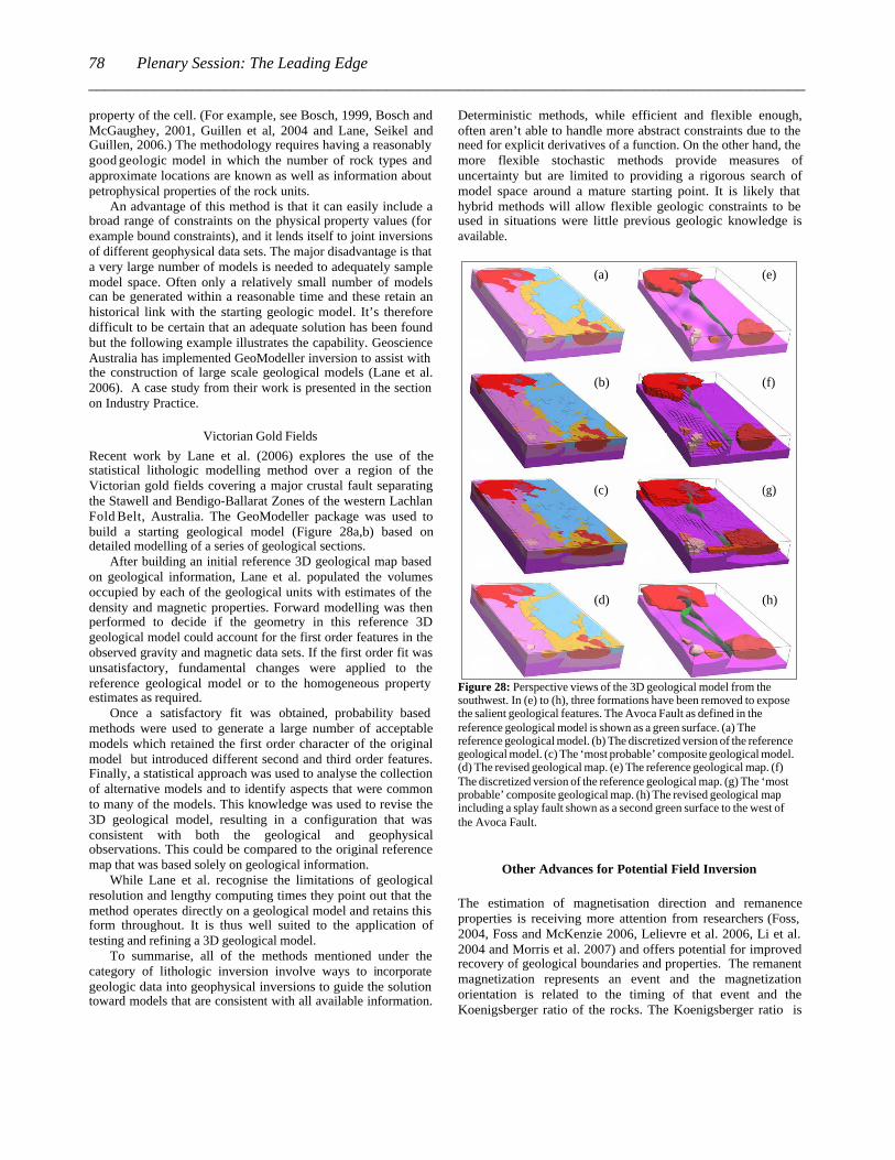
Recent work by Lane et al. (2006) explores the use of the statistical lithologic modelling method over a region of the Victorian gold fields covering a major crustal fault separating the Stawell and Bendigo-Ballarat Zones of the western Lachlan Fold Belt, Australia. The GeoModeller package was used to build a starting geological model (Figure 28a,b) based on detailed modelling of a series of geological sections.

After building an initial reference 3D geological map based on geological information, Lane et al. populated the volumes occupied by each of the geological units with estimates of the density and magnetic properties. Forward modelling was then performed to decide if the geometry in this reference 3D geological model could account for the first order features in the observed gravity and magnetic data sets. If the first order fit was unsatisfactory, fundamental changes were applied to the reference geological model or to the homogeneous property estimates as required.

Once a satisfactory fit was obtained, probability based methods were used to generate a large number of acceptable models which retained the first order character of the original model but introduced different second and third order features. Finally, a statistical approach was used to analyse the collection of alternative models and to identify aspects that were common to many of the models. This knowledge was used to revise the 3D geological model, resulting in a configuration that was consistent with both the geological and geophysical observations. This could be compared to the original reference map that was based solely on geological information.

While Lane et al. recognise the limitations of geological resolution and lengthy computing times they point out that the method operates directly on a geological model and retains this form throughout. It is thus well suited to the application of testing and refining a 3D geological model.

To summarise, all of the methods mentioned under the category of lithologic inversion involve ways to incorporate geologic data into geophysical inversions to guide the solution toward models that are consistent with all available information.

Deterministic methods, while efficient and flexible enough, often aren’t able to handle more abstract constraints due to the need for explicit derivatives of a function. On the other hand, the more flexible stochastic methods provide measures of uncertainty but are limited to providing a rigorous search of model space around a mature starting point. It is likely that hybrid methods will allow flexible geologic constraints to be used in situations were little previous geologic knowledge is available.

Figure 28: Perspective views of the 3D geological model from the southwest. In (e) to (h), three formations have been removed to expose the salient geological features. The Avoca Fault as defined in the reference geological model is shown as a green surface. (a) The reference geological model. (b) The discretized version of the reference geological model. (c) The ‘most probable’ composite geological model. (d) The revised geological map. (e) The reference geological map. (f) The discretized version of the reference geological map. (g) The ‘most probable’ composite geological map. (h) The revised geological map including a splay fault shown as a second green surface to the west of the Avoca Fault.

Other Advances for Potential Field Inversion

The estimation of magnetisation direction and remanence properties is receiving more attention from researchers (Foss, 2004, Foss and McKenzie 2006, Lelievre et al. 2006, Li et al. 2004 and Morris et al. 2007) and offers potential for improved recovery of geological boundaries and properties. The remanent magnetization represents an event and the magnetization orientation is related to the timing of that event and the Koenigsberger ratio of the rocks. The Koenigsberger ratio is

(a)

(b)

(c)

(d)

(e)

(f)

(g)

(h)


related to the mineral composition and physical properties of the rocks. Resolution of all three parameters has the potential to provide additional diagnostic information in greenfields exploration. Foss and McKenzie (2006) published an example for the Black Hill Norite where they compared direct polyhedral inversion with the Helbig method (Helbig 1963) and physical property measurements by Rajagopalan et al. (1993), and Schmidt and Clark (1998).

For highly magnetic bodies (susceptibility greater than about 0.3 SI) it is well known that self-demagnetization effects should be included in the forward modelling (Clark and Emerson, 1999). Under such circumstances the forward problem is no longer linear but an equation, similar to that needed for DC resistivity modelling must be solved. The most common way to incorporate self-demagnetization is through Type I algorithms where the body has a particular shape and demagnetization factors (Lee, 1980). Lelievre and Oldenburg (2006) present the details of a Type II inversion algorithm to recover the susceptibility of highly magnetic objects. It is envisaged that these methods will see more use over the next decade.

Gravity and magnetic data essentially use the earth as a generating source and hence there is only one data map for any component of the field. Forward modelling is straight forward and consequently a variety of tactics for solving the inverse problem have been advocated. Also, there is a fairly intuitive understanding about the relationship between the causative model and the data. This has made data maps useful for geologic interpretation. However, in active source surveys where there is a data map for each source and/or each field component, the situation is more complicated and inversion is a necessity. The next survey type, DC resistivity and IP (Induced Polarization), illustrates this.

INVERSION OF DC RESISTIVITY AND IP DATA

DC resistivity and IP are important survey techniques for mineral prospecting (See Zonge, Wynn and Urquhart, 2005, and the references there in). An electrical current I is the injected into the ground and electric potential is measured away from the source. The physical property of interest is the electrical conductivity s which is often observed to be frequency dependent (or equivalently time varying). The governing equations are Maxwell’s equations at zero frequency. Forward modelling for electric potentials is achieved by solving the equations with finite volume methods (Dey and Morrison, 1979) or using finite element or integral equation techniques. Data can be inverted using any of the strategies mentioned earlier. For the work presented here we shall restrict ourselves to the Type II strategy. Also, when inverting resistivity data we let m=logs, and a use the Gauss-Newton strategy outlined earlier. Although the complex conductivity can be solved for, it is more usual to break the problem into two parts. Consider for example a time domain current source that is a square wave with a 50% duty cycle. The primary potentials achieved just prior to shut-off are inverted to recover a conductivity distribution. Some aspect of the secondary potentials measured in the off-time, are used to invert for chargeability. The sensitivity J associated with the conductivity obtained from inverting DC resistivity data is used

for forward modelling induced polarization data. The relationship is Jh=d where h is the chargeability which has the same units as the IP data (e.g. mrad, msec). In the inversion h is restricted to be positive. There are many papers on this subject. See for example Fink, 1990 or Oldenburg and Li, 1994.

One of the first applications of 2D inversion to mineral exploration was for the Century zinc deposit, located approximately 250 km north-northwest of Mt. Isa in northwest Queensland, Australia (Mutton, 1997). Mineralization occurs preferentially within black shale units as fine-grained sphalerite and galena with minor pyrite. An apparent resistivity pseudo-section is shown in Figure 29. Prior to inversion capability the standard method for interpreting these data was to make inferences using compilations of pseudo-sections. Each datum however represents a global average of the conductivity and the volume of sensitivity is dependent upon locations of current and receiver electrodes. It is only under rare circumstances that the data image resembled the geology.

Figure 29: Resistivity and IP pseudo-sections are shown in (a) and (b) respectively. The recovered conductivity and chargeability are shown in (c) and (d), with base-of-limestone (white), faults (black), and mineralized stratigraphic units (dashed) superimposed.

The 177 data measurements were inverted using the algorithm described by Oldenburg and Li (1994). The earth was assumed to be 2D and divided into 2000 cells. The DC resistivity data were assigned a 3 percent error, and the objective function was designed to generate a model that was equally smooth in the horizontal and vertical directions and tended to return to a reference model of 10 Wm at depth, where the data no longer constrained the model. The recovered model is shown in Figure 29c along with a superimposed geologic section. The


79

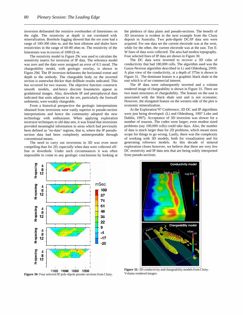
inversion delineated the resistive overburden of limestones on the right. The resistivity at depth is not correlated with mineralization. Borehole logging showed that the ore zone had a range of 100-300 ohm m, and the host siltstone and shales have resistivities in the range of 60-80 ohm-m. The resistivity of the limestones was in excess of 1000 W-m.

The resistivity model in Figure 29c was used to calculate the sensitivity matrix for inversion of IP data. The reference model was zero and the data were assigned an error of 0.5 mrad. The chargeability model, with geologic overlay, is shown in Figure 29d. The IP inversion delineates the horizontal extent and depth to the orebody. The chargeable body on the inverted section is somewhat thicker than drillhole results indicated. This has occurred for two reasons. The objective function constructs smooth models, and hence discrete boundaries appear as gradational images. Also, downhole IP and petrophysical data indicated that units adjacent to the ore, particularly the footwall sediments, were weakly chargeable.

From a historical perspective the geologic interpretations obtained from inversions were vastly superior to pseudo-section interpretations and hence the community adopted the new technology with enthusiasm. When applying exploration inversion techniques to old data sets, it was found that inversions provided meaningful information in areas which had previously been defined as "no-data" regions, that is, where the IP pseudo-section data had been completely uninterpretable through conventional means.

The need to carry out inversions in 3D was even more compelling than for 2D, especially when data were collected off-line or downhole. Under such circumstances it was often impossible to come to any geologic conclusions by looking at

the plethora of data plans and pseudo-sections. The benefit of 3D inversion is evident in the next example from the Cluny deposit in Australia. Two pole-dipole DC/IP data sets were acquired. For one data set the current electrode was at the west, while for the other, the current electrode was at the east. Ten E-W lines of data were collected. The area had modest topography. Four selected lines of IP data are shown in Figure 30.

The DC data were inverted to recover a 3D cube of conductivity that had 180,000 cells. The algorithm used was the Gauss-Newton algorithm described in Li and Oldenburg, 2000. A plan view of the conductivity, at a depth of 375m is shown in Figure 31. The dominant feature is a graphitic black shale in the east which is of no commercial interest.

The IP data were subsequently inverted and a volume rendered image of chargeability is shown in Figure 31. There are two main structures of chargeability. The feature on the east is associated with the black shale unit and is not economic. However, the elongated feature on the western side of the plot is economic mineralization.

At the Exploration’97 Conference, 3D DC and IP algorithms were just being developed. (Li and Oldenburg, 1997 Loke and Dahlin, 1997). Acceptance of 3D inversion was slower for a number of reasons. The codes were larger; even modest sized problems (say 100,000 cells) could take days. Also, the number of data is much larger than for 2D problems, which meant more scope for things to go wrong. Lastly, there was the complexity of working with 3D models, both for visualization and for generating reference models. As this decade of mineral exploration closes however, we believe that there are very few DC resistivity and IP data sets that are being solely interpreted from pseudo-sections.

Figure 30: Four selected IP pole-dipole pseudo-sections from Cluny.

Figure 31: 3D conductivity and chargeability models from Cluny. Volume rendered images.


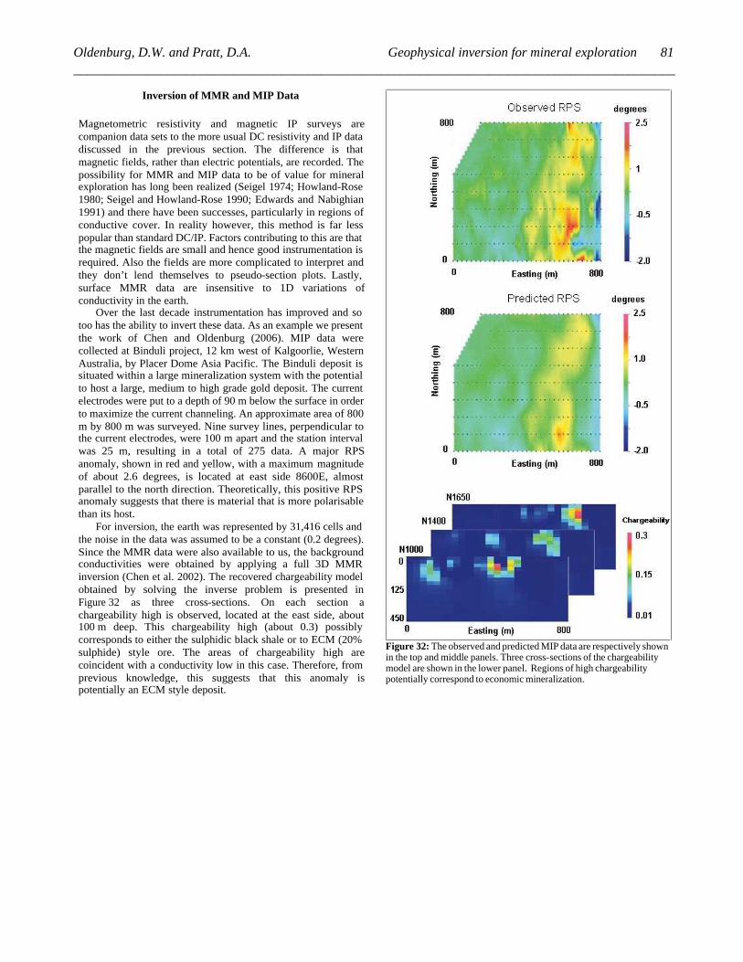
Inversion of MMR and MIP Data

Magnetometric resistivity and magnetic IP surveys are companion data sets to the more usual DC resistivity and IP data discussed in the previous section. The difference is that magnetic fields, rather than electric potentials, are recorded. The possibility for MMR and MIP data to be of value for mineral exploration has long been realized (Seigel 1974; Howland-Rose 1980; Seigel and Howland-Rose 1990; Edwards and Nabighian 1991) and there have been successes, particularly in regions of conductive cover. In reality however, this method is far less popular than standard DC/IP. Factors contributing to this are that the magnetic fields are small and hence good instrumentation is required. Also the fields are more complicated to interpret and they don’t lend themselves to pseudo-section plots. Lastly, surface MMR data are insensitive to 1D variations of conductivity in the earth.

Over the last decade instrumentation has improved and so too has the ability to invert these data. As an example we present the work of Chen and Oldenburg (2006). MIP data were collected at Binduli project, 12 km west of Kalgoorlie, Western Australia, by Placer Dome Asia Pacific. The Binduli deposit is situated within a large mineralization system with the potential to host a large, medium to high grade gold deposit. The current electrodes were put to a depth of 90 m below the surface in order to maximize the current channeling. An approximate area of 800 m by 800 m was surveyed. Nine survey lines, perpendicular to the current electrodes, were 100 m apart and the station interval was 25 m, resulting in a total of 275 data. A major RPS anomaly, shown in red and yellow, with a maximum magnitude of about 2.6 degrees, is located at east side 8600E, almost parallel to the north direction. Theoretically, this positive RPS anomaly suggests that there is material that is more polarisable than its host.

For inversion, the earth was represented by 31,416 cells and the noise in the data was assumed to be a constant (0.2 degrees). Since the MMR data were also available to us, the background conductivities were obtained by applying a full 3D MMR inversion (Chen et al. 2002). The recovered chargeability model obtained by solving the inverse problem is presented in Figure 32 as three cross-sections. On each section a chargeability high is observed, located at the east side, about 100 m deep. This chargeability high (about 0.3) possibly corresponds to either the sulphidic black shale or to ECM (20% sulphide) style ore. The areas of chargeability high are coincident with a conductivity low in this case. Therefore, from previous knowledge, this suggests that this anomaly is potentially an ECM style deposit.

Figure 32: The observed and predicted MIP data are respectively shown in the top and middle panels. Three cross-sections of the chargeability model are shown in the lower panel. Regions of high chargeability potentially correspond to economic mineralization.


81

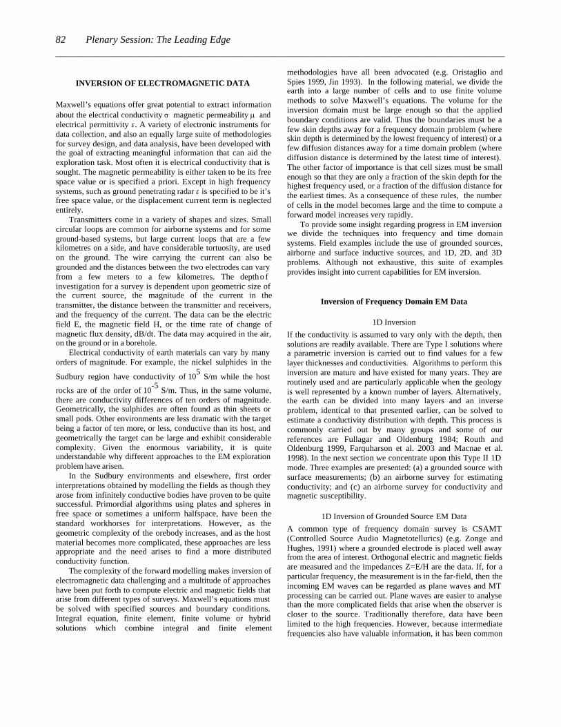
INVERSION OF ELECTROMAGNETIC DATA

Maxwell’s equations offer great potential to extract information about the electrical conductivity s magnetic permeability m and electrical permittivity ε. A variety of electronic instruments for data collection, and also an equally large suite of methodologies for survey design, and data analysis, have been developed with the goal of extracting meaningful information that can aid the exploration task. Most often it is electrical conductivity that is sought. The magnetic permeability is either taken to be its free space value or is specified a priori. Except in high frequency systems, such as ground penetrating radar ε is specified to be it’s free space value, or the displacement current term is neglected entirely.

Transmitters come in a variety of shapes and sizes. Small circular loops are common for airborne systems and for some ground-based systems, but large current loops that are a few kilometres on a side, and have considerable tortuosity, are used on the ground. The wire carrying the current can also be grounded and the distances between the two electrodes can vary from a few meters to a few kilometres. The depth o f investigation for a survey is dependent upon geometric size of the current source, the magnitude of the current in the transmitter, the distance between the transmitter and receivers, and the frequency of the current. The data can be the electric field E, the magnetic field H, or the time rate of change of magnetic flux density, dB/dt. The data may acquired in the air, on the ground or in a borehole.

Electrical conductivity of earth materials can vary by many orders of magnitude. For example, the nickel sulphides in the

Sudbury region have conductivity of 105 S/m while the host

rocks are of the order of 10-5

S/m. Thus, in the same volume, there are conductivity differences of ten orders of magnitude. Geometrically, the sulphides are often found as thin sheets or small pods. Other environments are less dramatic with the target being a factor of ten more, or less, conductive than its host, and geometrically the target can be large and exhibit considerable complexity. Given the enormous variability, it is quite understandable why different approaches to the EM exploration problem have arisen.

In the Sudbury environments and elsewhere, first order interpretations obtained by modelling the fields as though they arose from infinitely conductive bodies have proven to be quite successful. Primordial algorithms using plates and spheres in free space or sometimes a uniform halfspace, have been the standard workhorses for interpretations. However, as the geometric complexity of the orebody increases, and as the host material becomes more complicated, these approaches are less appropriate and the need arises to find a more distributed conductivity function.

The complexity of the forward modelling makes inversion of electromagnetic data challenging and a multitude of approaches have been put forth to compute electric and magnetic fields that arise from different types of surveys. Maxwell’s equations must be solved with specified sources and boundary conditions. Integral equation, finite element, finite volume or hybrid solutions which combine integral and finite element

methodologies have all been advocated (e.g. Oristaglio and Spies 1999, Jin 1993). In the following material, we divide the earth into a large number of cells and to use finite volume methods to solve Maxwell’s equations. The volume for the inversion domain must be large enough so that the applied boundary conditions are valid. Thus the boundaries must be a few skin depths away for a frequency domain problem (where skin depth is determined by the lowest frequency of interest) or a few diffusion distances away for a time domain problem (where diffusion distance is determined by the latest time of interest). The other factor of importance is that cell sizes must be small enough so that they are only a fraction of the skin depth for the highest frequency used, or a fraction of the diffusion distance for the earliest times. As a consequence of these rules, the number of cells in the model becomes large and the time to compute a forward model increases very rapidly.

To provide some insight regarding progress in EM inversion we divide the techniques into frequency and time domain systems. Field examples include the use of grounded sources, airborne and surface inductive sources, and 1D, 2D, and 3D problems. Although not exhaustive, this suite of examples provides insight into current capabilities for EM inversion.

Inversion of Frequency Domain EM Data

1D Inversion

If the conductivity is assumed to vary only with the depth, then solutions are readily available. There are Type I solutions where a parametric inversion is carried out to find values for a few layer thicknesses and conductivities. Algorithms to perform this inversion are mature and have existed for many years. They are routinely used and are particularly applicable when the geology is well represented by a known number of layers. Alternatively, the earth can be divided into many layers and an inverse problem, identical to that presented earlier, can be solved to estimate a conductivity distribution with depth. This process is commonly carried out by many groups and some of our references are Fullagar and Oldenburg 1984; Routh and Oldenburg 1999, Farquharson et al. 2003 and Macnae et al. 1998). In the next section we concentrate upon this Type II 1D mode. Three examples are presented: (a) a grounded source with surface measurements; (b) an airborne survey for estimating conductivity; and (c) an airborne survey for conductivity and magnetic susceptibility.

1D Inversion of Grounded Source EM Data

A common type of frequency domain survey is CSAMT (Controlled Source Audio Magnetotellurics) (e.g. Zonge and Hughes, 1991) where a grounded electrode is placed well away from the area of interest. Orthogonal electric and magnetic fields are measured and the impedances Z=E/H are the data. If, for a particular frequency, the measurement is in the far-field, then the incoming EM waves can be regarded as plane waves and MT processing can be carried out. Plane waves are easier to analyse than the more complicated fields that arise when the observer is closer to the source. Traditionally therefore, data have been limited to the high frequencies. However, because intermediate frequencies also have valuable information, it has been common


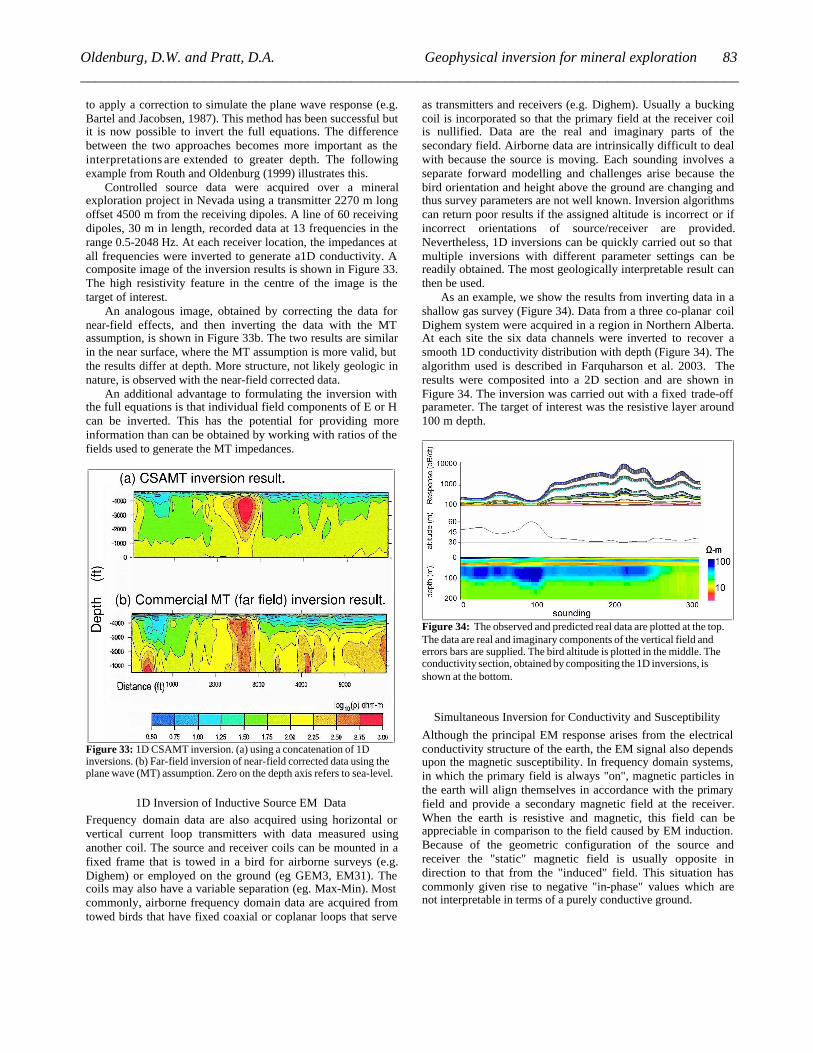
to apply a correction to simulate the plane wave response (e.g. Bartel and Jacobsen, 1987). This method has been successful but it is now possible to invert the full equations. The difference between the two approaches becomes more important as the interpretations are extended to greater depth. The following example from Routh and Oldenburg (1999) illustrates this.

Controlled source data were acquired over a mineral exploration project in Nevada using a transmitter 2270 m long offset 4500 m from the receiving dipoles. A line of 60 receiving dipoles, 30 m in length, recorded data at 13 frequencies in the range 0.5-2048 Hz. At each receiver location, the impedances at all frequencies were inverted to generate a1D conductivity. A composite image of the inversion results is shown in Figure 33. The high resistivity feature in the centre of the image is the target of interest.

An analogous image, obtained by correcting the data for near-field effects, and then inverting the data with the MT assumption, is shown in Figure 33b. The two results are similar in the near surface, where the MT assumption is more valid, but the results differ at depth. More structure, not likely geologic in nature, is observed with the near-field corrected data.

An additional advantage to formulating the inversion with the full equations is that individual field components of E or H can be inverted. This has the potential for providing more information than can be obtained by working with ratios of the fields used to generate the MT impedances.

Figure 33: 1D CSAMT inversion. (a) using a concatenation of 1D inversions. (b) Far-field inversion of near-field corrected data using the plane wave (MT) assumption. Zero on the depth axis refers to sea-level.

1D Inversion of Inductive Source EM Data

Frequency domain data are also acquired using horizontal or vertical current loop transmitters with data measured using another coil. The source and receiver coils can be mounted in a fixed frame that is towed in a bird for airborne surveys (e.g. Dighem) or employed on the ground (eg GEM3, EM31). The coils may also have a variable separation (eg. Max-Min). Most commonly, airborne frequency domain data are acquired from towed birds that have fixed coaxial or coplanar loops that serve

as transmitters and receivers (e.g. Dighem). Usually a bucking coil is incorporated so that the primary field at the receiver coil is nullified. Data are the real and imaginary parts of the secondary field. Airborne data are intrinsically difficult to deal with because the source is moving. Each sounding involves a separate forward modelling and challenges arise because the bird orientation and height above the ground are changing and thus survey parameters are not well known. Inversion algorithms can return poor results if the assigned altitude is incorrect or if incorrect orientations of source/receiver are provided. Nevertheless, 1D inversions can be quickly carried out so that multiple inversions with different parameter settings can be readily obtained. The most geologically interpretable result can then be used.

As an example, we show the results from inverting data in a shallow gas survey (Figure 34). Data from a three co-planar coil Dighem system were acquired in a region in Northern Alberta. At each site the six data channels were inverted to recover a smooth 1D conductivity distribution with depth (Figure 34). The algorithm used is described in Farquharson et al. 2003. The results were composited into a 2D section and are shown in Figure 34. The inversion was carried out with a fixed trade-off parameter. The target of interest was the resistive layer around 100 m depth.

Figure 34: The observed and predicted real data are plotted at the top. The data are real and imaginary components of the vertical field and errors bars are supplied. The bird altitude is plotted in the middle. The conductivity section, obtained by compositing the 1D inversions, is shown at the bottom.

Simultaneous Inversion for Conductivity and Susceptibility

Although the principal EM response arises from the electrical conductivity structure of the earth, the EM signal also depends upon the magnetic susceptibility. In frequency domain systems, in which the primary field is always "on", magnetic particles in the earth will align themselves in accordance with the primary field and provide a secondary magnetic field at the receiver. When the earth is resistive and magnetic, this field can be appreciable in comparison to the field caused by EM induction. Because of the geometric configuration of the source and receiver the "static" magnetic field is usually opposite in direction to that from the "induced" field. This situation has commonly given rise to negative "in-phase" values which are not interpretable in terms of a purely conductive ground.


83

The importance of magnetic susceptibility has long been recognized (e.g. Fraser, 1973, 1981) but most approaches have centred around finding a magnetic halfspace, or a layer over a halfspace, to account for the responses (e.g. Beard and Nyquist, 1998). However, it is possible to invert for magnetic susceptibility in the same way as electrical conductivity. Frequency domain EM data can be inverted to recover only susceptibility in those cases where the electrical conductivity is negligible, or to simultaneously recover conductivity and susceptibility (Zhang and Oldenburg 1999; Farquharson et al. 2003). Figure 35 shows a line of airborne data collected at Heathe Steele Stratmat in the Bathurst region. The region has highly conductive and magnetically susceptible massive sulphide deposits, and magnetically susceptible gabbro dikes. The flight line passes close to one of the massive sulphide deposits. Observations were made at 946 and 4575 Hz with a coaxial coil configuration and at 4175 Hz for a horizontal coplanar coil configuration. Transmitter and receiver coils were separated by about 7m and the bird height was about 40m. The observed and predicted data, and the 2D images of conductivity and susceptibility are shown in Figure 35 with the target body superimposed. Although there are clearly artefacts that arise because of imaging a 3D body with a 1D code, the inversion result has been quite useful in delineating the location of the sulphide.

Figure 35: Simultaneous conductivity and susceptibility 1D inversion of frequency domain airborne EM data. The top panel shows observed and predicted in-phase and quadrature-phase data. Note that some of the in-phase data are negative. Sections of conductivity and magnetic

susceptibility, obtained from compositing the 1D inversions, are shown in the lower panels. An image of the massive sulphide deposit is overlaid.

The inversion was performed on successive lines in the region and a 3D susceptibility model was generated. That model is shown in Figure 36 as a volume rendered image with a cutoff of 0.35 SI. The image can be compared with the 3D susceptibility obtained by inverting ground magnetic data. The volume rendered image is shown with a cutoff of 0.2 SI. The values of susceptibility in the model constructed from EM data are generally larger than those resulting from the inversion of magnetic data. Nevertheless there is good agreement between the features in the two models: the region of susceptibility encompassing the mineralized zone and the east-west trending susceptible zone in the southern part of the model that is thought to correspond to a gabbro dyke.

Figure 36: Comparison of magnetic susceptibility from 1D inversions of EM data with that produced from a 3D magnetic inversion

To summarize this section, the 1D inversion of frequency

domain data is well advanced. There are many algorithms that can invert fields from airborne or surface surveys to recover the electrical conductivity. It is also possible to recover information about magnetic susceptibility from these same measurements. The benefits for simultaneous inversion are two fold: (a) the quality of the recovered conductivity model is greatly increased and (b) the recovered susceptibility can be useful as an additional interpretation aid.

3D Inversion in the Frequency Domain EM Data

Although 1D inversions are useful, mineral exploration problems are inherently 3D and hence it is necessary to work in higher dimensions. Some work has been done in 2D. For


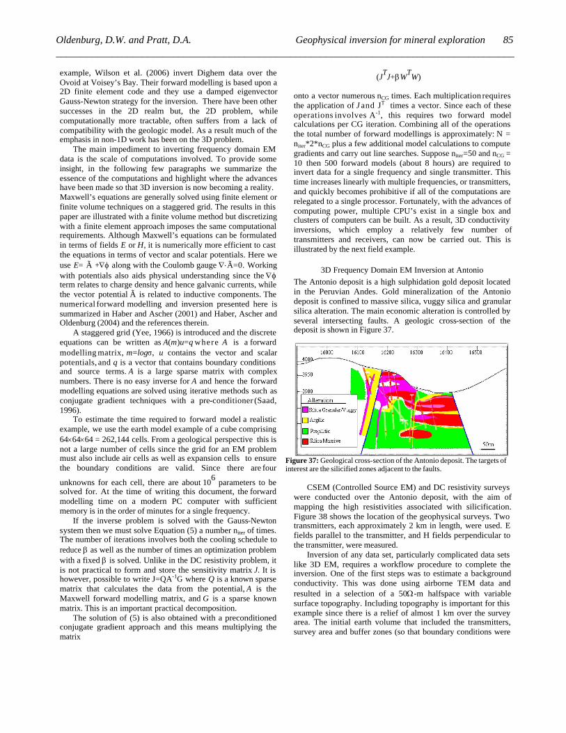
example, Wilson et al. (2006) invert Dighem data over the Ovoid at Voisey’s Bay. Their forward modelling is based upon a 2D finite element code and they use a damped eigenvector Gauss-Newton strategy for the inversion. There have been other successes in the 2D realm but, the 2D problem, while computationally more tractable, often suffers from a lack of compatibility with the geologic model. As a result much of the emphasis in non-1D work has been on the 3D problem.

The main impediment to inverting frequency domain EM data is the scale of computations involved. To provide some insight, in the following few paragraphs we summarize the essence of the computations and highlight where the advances have been made so that 3D inversion is now becoming a reality. Maxwell’s equations are generally solved using finite element or finite volume techniques on a staggered grid. The results in this paper are illustrated with a finite volume method but discretizing with a finite element approach imposes the same computational requirements. Although Maxwell’s equations can be formulated in terms of fields E or H, it is numerically more efficient to cast the equations in terms of vector and scalar potentials. Here we use E= Ã +Ñf along with the Coulomb gauge Ñ×Ã=0. Working with potentials also aids physical understanding since the Ñf term relates to charge density and hence galvanic currents, while the vector potential Ã is related to inductive components. The numerical forward modelling and inversion presented here is summarized in Haber and Ascher (2001) and Haber, Ascher and Oldenburg (2004) and the references therein.

A staggered grid (Yee, 1966) is introduced and the discrete equations can be written as A(m)u=q where A is a forward modelling matrix, m=logs, u contains the vector and scalar potentials, and q is a vector that contains boundary conditions and source terms. A is a large sparse matrix with complex numbers. There is no easy inverse for A and hence the forward modelling equations are solved using iterative methods such as conjugate gradient techniques with a pre-conditioner (Saad, 1996).

To estimate the time required to forward model a realistic example, we use the earth model example of a cube comprising 64´64´64 = 262,144 cells. From a geological perspective this is not a large number of cells since the grid for an EM problem must also include air cells as well as expansion cells to ensure the boundary conditions are valid. Since there are four

unknowns for each cell, there are about 106 parameters to be

solved for. At the time of writing this document, the forward modelling time on a modern PC computer with sufficient memory is in the order of minutes for a single frequency.

If the inverse problem is solved with the Gauss-Newton system then we must solve Equation (5) a number niter of times. The number of iterations involves both the cooling schedule to reduce b as well as the number of times an optimization problem with a fixed b is solved. Unlike in the DC resistivity problem, it is not practical to form and store the sensitivity matrix J. It is however, possible to write J=QA-1G where Q is a known sparse matrix that calculates the data from the potential, A is the Maxwell forward modelling matrix, and G is a sparse known matrix. This is an important practical decomposition.

The solution of (5) is also obtained with a preconditioned conjugate gradient approach and this means multiplying the matrix

(JT

J+bWTW)

onto a vector numerous nCG times. Each multiplication requires the application of J and JT times a vector. Since each of these operations involves A-1, this requires two forward model calculations per CG iteration. Combining all of the operations the total number of forward modellings is approximately: N = niter*2*nCG plus a few additional model calculations to compute gradients and carry out line searches. Suppose niter=50 and nCG = 10 then 500 forward models (about 8 hours) are required to invert data for a single frequency and single transmitter. This time increases linearly with multiple frequencies, or transmitters, and quickly becomes prohibitive if all of the computations are relegated to a single processor. Fortunately, with the advances of computing power, multiple CPU’s exist in a single box and clusters of computers can be built. As a result, 3D conductivity inversions, which employ a relatively few number of transmitters and receivers, can now be carried out. This is illustrated by the next field example.

3D Frequency Domain EM Inversion at Antonio

The Antonio deposit is a high sulphidation gold deposit located in the Peruvian Andes. Gold mineralization of the Antonio deposit is confined to massive silica, vuggy silica and granular silica alteration. The main economic alteration is controlled by several intersecting faults. A geologic cross-section of the deposit is shown in Figure 37.

Figure 37: Geological cross-section of the Antonio deposit. The targets of interest are the silicified zones adjacent to the faults.

CSEM (Controlled Source EM) and DC resistivity surveys

were conducted over the Antonio deposit, with the aim of mapping the high resistivities associated with silicification. Figure 38 shows the location of the geophysical surveys. Two transmitters, each approximately 2 km in length, were used. E fields parallel to the transmitter, and H fields perpendicular to the transmitter, were measured.

Inversion of any data set, particularly complicated data sets like 3D EM, requires a workflow procedure to complete the inversion. One of the first steps was to estimate a background conductivity. This was done using airborne TEM data and resulted in a selection of a 50W-m halfspace with variable surface topography. Including topography is important for this example since there is a relief of almost 1 km over the survey area. The initial earth volume that included the transmitters, survey area and buffer zones (so that boundary conditions were


85

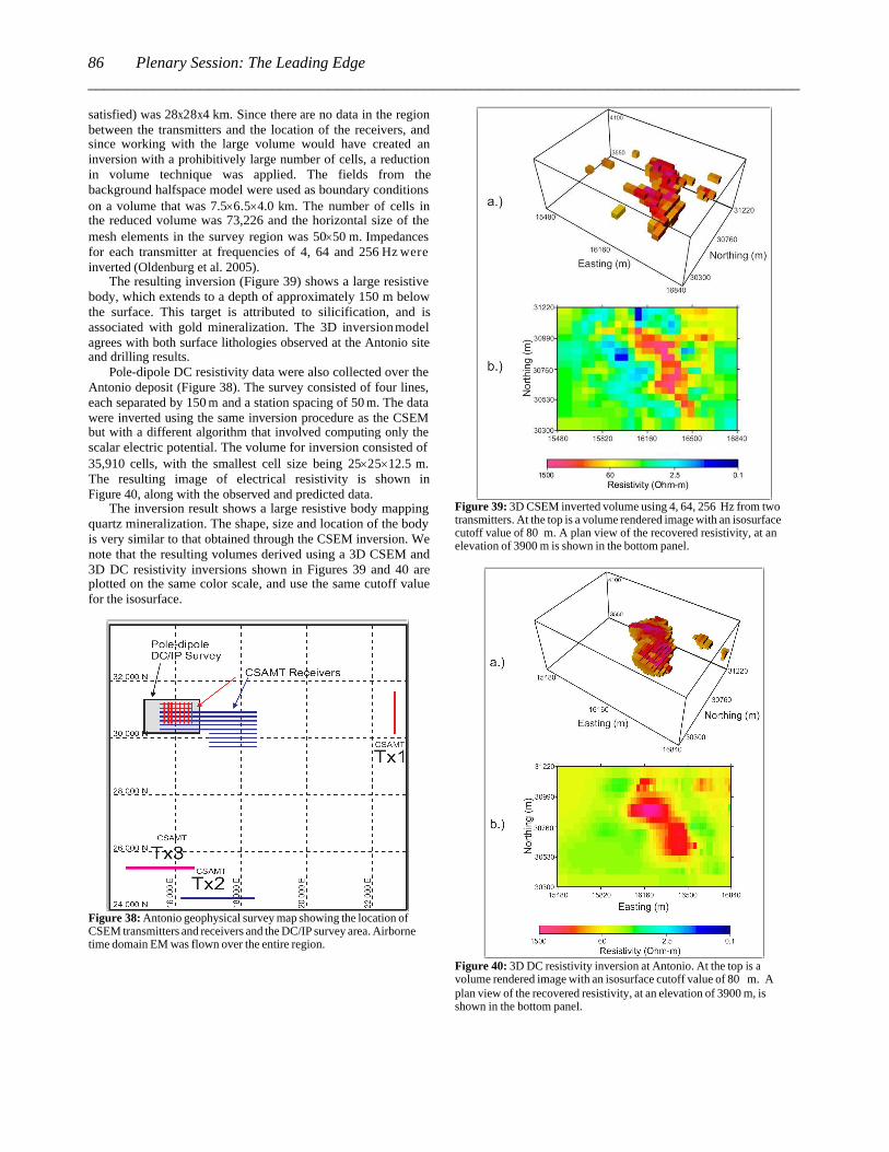
satisfied) was 28x28x4 km. Since there are no data in the region between the transmitters and the location of the receivers, and since working with the large volume would have created an inversion with a prohibitively large number of cells, a reduction in volume technique was applied. The fields from the background halfspace model were used as boundary conditions on a volume that was 7.5´6.5´4.0 km. The number of cells in the reduced volume was 73,226 and the horizontal size of the mesh elements in the survey region was 50´50 m. Impedances for each transmitter at frequencies of 4, 64 and 256 Hz were inverted (Oldenburg et al. 2005).

The resulting inversion (Figure 39) shows a large resistive body, which extends to a depth of approximately 150 m below the surface. This target is attributed to silicification, and is associated with gold mineralization. The 3D inversion model agrees with both surface lithologies observed at the Antonio site and drilling results.

Pole-dipole DC resistivity data were also collected over the Antonio deposit (Figure 38). The survey consisted of four lines, each separated by 150 m and a station spacing of 50 m. The data were inverted using the same inversion procedure as the CSEM but with a different algorithm that involved computing only the scalar electric potential. The volume for inversion consisted of 35,910 cells, with the smallest cell size being 25´25´12.5 m. The resulting image of electrical resistivity is shown in Figure 40, along with the observed and predicted data.

The inversion result shows a large resistive body mapping quartz mineralization. The shape, size and location of the body is very similar to that obtained through the CSEM inversion. We note that the resulting volumes derived using a 3D CSEM and 3D DC resistivity inversions shown in Figures 39 and 40 are plotted on the same color scale, and use the same cutoff value for the isosurface.

Figure 38: Antonio geophysical survey map showing the location of CSEM transmitters and receivers and the DC/IP survey area. Airborne time domain EM was flown over the entire region.

Figure 39: 3D CSEM inverted volume using 4, 64, 256 Hz from two transmitters. At the top is a volume rendered image with an isosurface cutoff value of 80 m. A plan view of the recovered resistivity, at an elevation of 3900 m is shown in the bottom panel.

Figure 40: 3D DC resistivity inversion at Antonio. At the top is a volume rendered image with an isosurface cutoff value of 80 m. A plan view of the recovered resistivity, at an elevation of 3900 m, is shown in the bottom panel.


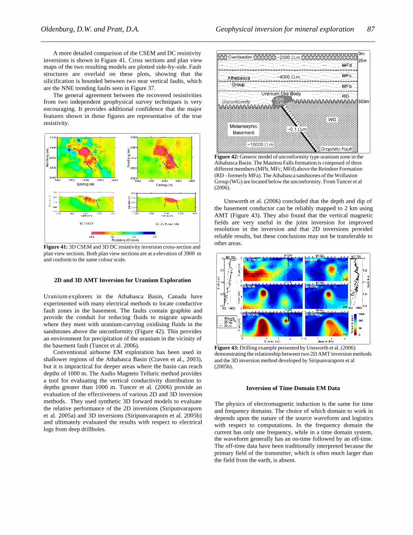
A more detailed comparison of the CSEM and DC resistivity inversions is shown in Figure 41. Cross sections and plan view maps of the two resulting models are plotted side-by-side. Fault structures are overlaid on these plots, showing that the silicification is bounded between two near vertical faults, which are the NNE trending faults seen in Figure 37.

The general agreement between the recovered resistivities from two independent geophysical survey techniques is very encouraging. It provides additional confidence that the major features shown in those figures are representative of the true resistivity.

Figure 41: 3D CSEM and 3D DC resistivity inversion cross-section and plan view sections. Both plan view sections are at a elevation of 3900 m and conform to the same colour scale.

2D and 3D AMT Inversion for Uranium Exploration

Uranium explorers in the Athabasca Basin, Canada have experimented with many electrical methods to locate conductive fault zones in the basement. The faults contain graphite and provide the conduit for reducing fluids to migrate upwards where they meet with uranium-carrying oxidising fluids in the sandstones above the unconformity (Figure 42). This provides an environment for precipitation of the uranium in the vicinity of the basement fault (Tuncer et al. 2006).

Conventional airborne EM exploration has been used in shallower regions of the Athabasca Basin (Craven et al., 2003), but it is impractical for deeper areas where the basin can reach depths of 1000 m. The Audio Magneto Telluric method provides a tool for evaluating the vertical conductivity distribution to depths greater than 1000 m. Tuncer et al. (2006) provide an evaluation of the effectiveness of various 2D and 3D inversion methods. They used synthetic 3D forward models to evaluate the relative performance of the 2D inversions (Siripunvaraporn et al. 2005a) and 3D inversions (Siripunvaraporn et al. 2005b) and ultimately evaluated the results with respect to electrical logs from deep drillholes.

Figure 42: Generic model of unconformity type uranium zone in the Athabasca Basin. The Manitou Falls formation is composed of three different members (MFb, MFc, MFd) above the Reindeer Formation (RD - formerly MFa). The Athabasca sandstones of the Wollaston Group (WG) are located below the unconformity. From Tuncer et al (2006).

Unsworth et al. (2006) concluded that the depth and dip of the basement conductor can be reliably mapped to 2 km using AMT (Figure 43). They also found that the vertical magnetic fields are very useful in the joint inversion for improved resolution in the inversion and that 2D inversions provided reliable results, but these conclusions may not be transferable to other areas.

Figure 43: Drilling example presented by Unsworth et al. (2006) demonstrating the relationship between two 2D AMT inversion methods and the 3D inversion method developed by Siripunvaraporn et al (2005b).

Inversion of Time Domain EM Data

The physics of electromagnetic induction is the same for time and frequency domains. The choice of which domain to work in depends upon the nature of the source waveform and logistics with respect to computations. In the frequency domain the current has only one frequency, while in a time domain system, the waveform generally has an on-time followed by an off-time. The off-time data have been traditionally interpreted because the primary field of the transmitter, which is often much larger than the field from the earth, is absent.


87

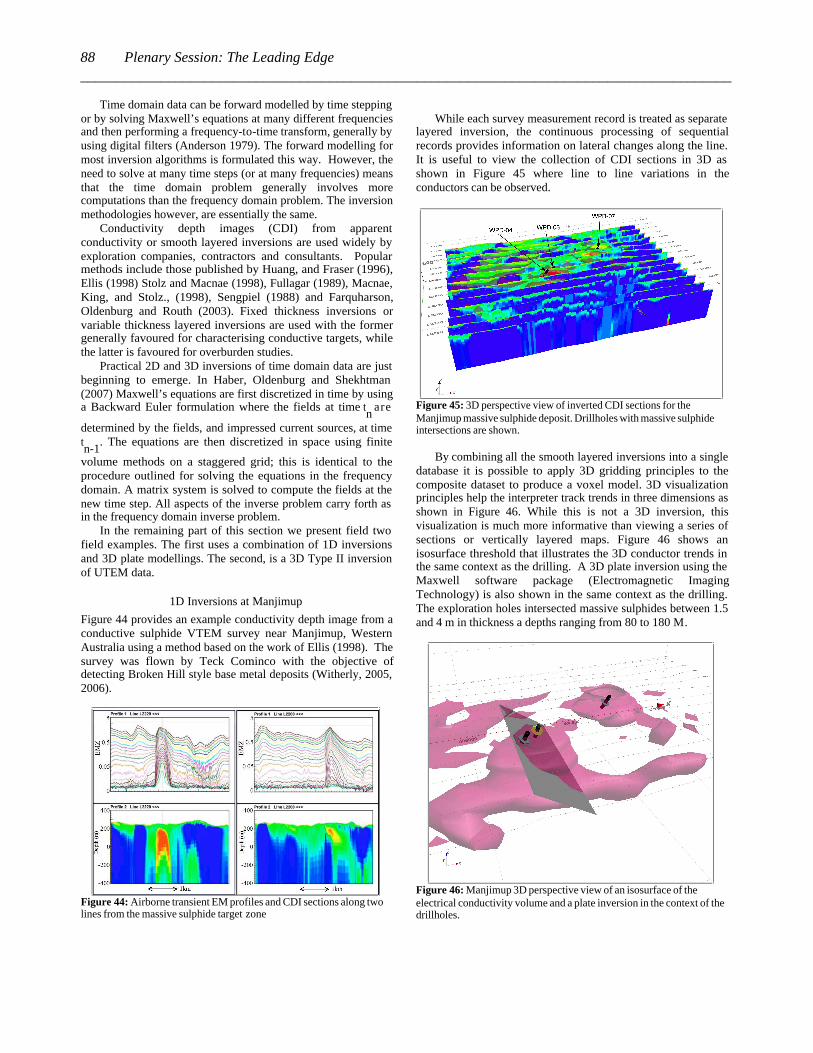
Time domain data can be forward modelled by time stepping or by solving Maxwell’s equations at many different frequencies and then performing a frequency-to-time transform, generally by using digital filters (Anderson 1979). The forward modelling for most inversion algorithms is formulated this way. However, the need to solve at many time steps (or at many frequencies) means that the time domain problem generally involves more computations than the frequency domain problem. The inversion methodologies however, are essentially the same.

Conductivity depth images (CDI) from apparent conductivity or smooth layered inversions are used widely by exploration companies, contractors and consultants. Popular methods include those published by Huang, and Fraser (1996), Ellis (1998) Stolz and Macnae (1998), Fullagar (1989), Macnae, King, and Stolz., (1998), Sengpiel (1988) and Farquharson, Oldenburg and Routh (2003). Fixed thickness inversions or variable thickness layered inversions are used with the former generally favoured for characterising conductive targets, while the latter is favoured for overburden studies.

Practical 2D and 3D inversions of time domain data are just beginning to emerge. In Haber, Oldenburg and Shekhtman (2007) Maxwell’s equations are first discretized in time by using a Backward Euler formulation where the fields at time t

n are

determined by the fields, and impressed current sources, at time tn-1

. The equations are then discretized in space using finite

volume methods on a staggered grid; this is identical to the procedure outlined for solving the equations in the frequency domain. A matrix system is solved to compute the fields at the new time step. All aspects of the inverse problem carry forth as in the frequency domain inverse problem.

In the remaining part of this section we present field two field examples. The first uses a combination of 1D inversions and 3D plate modellings. The second, is a 3D Type II inversion of UTEM data.

1D Inversions at Manjimup

Figure 44 provides an example conductivity depth image from a conductive sulphide VTEM survey near Manjimup, Western Australia using a method based on the work of Ellis (1998). The survey was flown by Teck Cominco with the objective of detecting Broken Hill style base metal deposits (Witherly, 2005, 2006).

Figure 44: Airborne transient EM profiles and CDI sections along two lines from the massive sulphide target zone

While each survey measurement record is treated as separate

layered inversion, the continuous processing of sequential records provides information on lateral changes along the line. It is useful to view the collection of CDI sections in 3D as shown in Figure 45 where line to line variations in the conductors can be observed.

Figure 45: 3D perspective view of inverted CDI sections for the Manjimup massive sulphide deposit. Drillholes with massive sulphide intersections are shown.

By combining all the smooth layered inversions into a single database it is possible to apply 3D gridding principles to the composite dataset to produce a voxel model. 3D visualization principles help the interpreter track trends in three dimensions as shown in Figure 46. While this is not a 3D inversion, this visualization is much more informative than viewing a series of sections or vertically layered maps. Figure 46 shows an isosurface threshold that illustrates the 3D conductor trends in the same context as the drilling. A 3D plate inversion using the Maxwell software package (Electromagnetic Imaging Technology) is also shown in the same context as the drilling. The exploration holes intersected massive sulphides between 1.5 and 4 m in thickness a depths ranging from 80 to 180 M.

Figure 46: Manjimup 3D perspective view of an isosurface of the electrical conductivity volume and a plate inversion in the context of the drillholes.


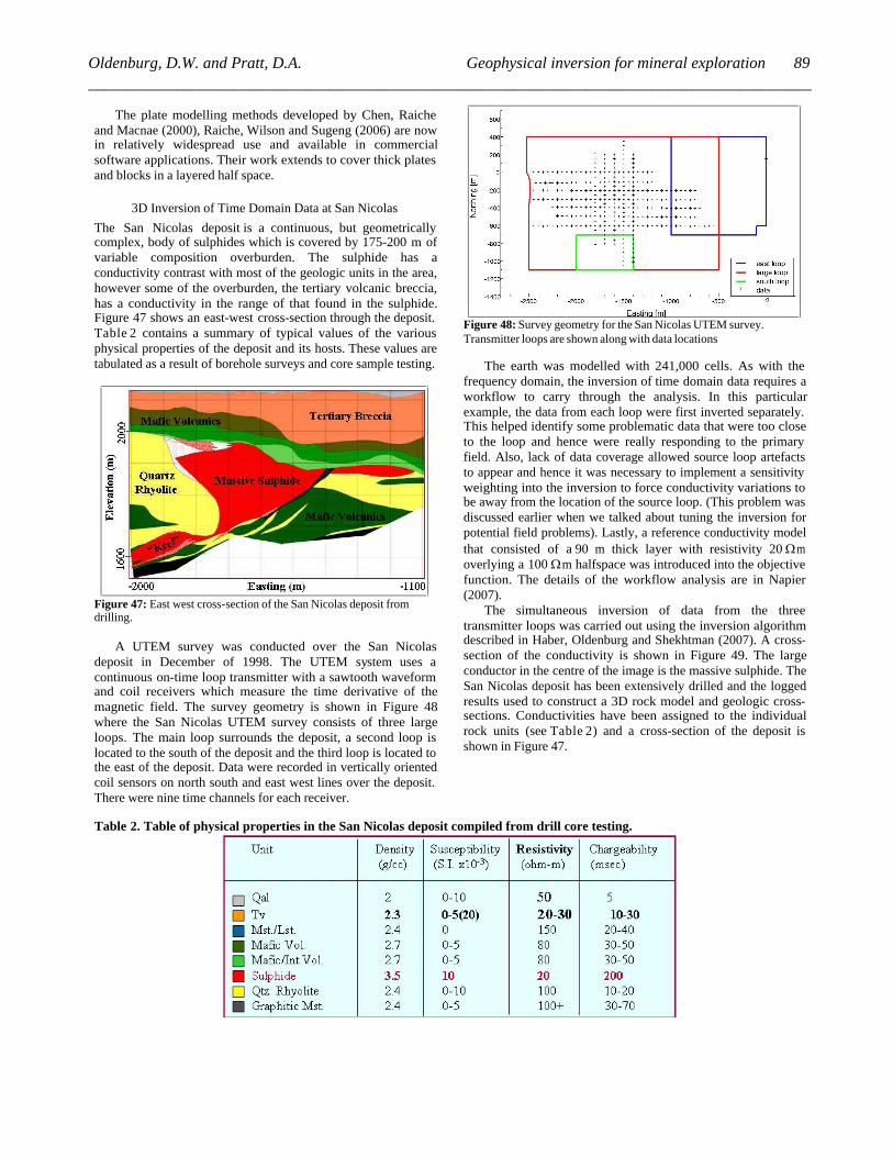
The plate modelling methods developed by Chen, Raiche and Macnae (2000), Raiche, Wilson and Sugeng (2006) are now in relatively widespread use and available in commercial software applications. Their work extends to cover thick plates and blocks in a layered half space.

3D Inversion of Time Domain Data at San Nicolas

The San Nicolas deposit is a continuous, but geometrically complex, body of sulphides which is covered by 175-200 m of variable composition overburden. The sulphide has a conductivity contrast with most of the geologic units in the area, however some of the overburden, the tertiary volcanic breccia, has a conductivity in the range of that found in the sulphide. Figure 47 shows an east-west cross-section through the deposit. Table 2 contains a summary of typical values of the various physical properties of the deposit and its hosts. These values are tabulated as a result of borehole surveys and core sample testing.

Figure 47: East west cross-section of the San Nicolas deposit from drilling.

A UTEM survey was conducted over the San Nicolas deposit in December of 1998. The UTEM system uses a continuous on-time loop transmitter with a sawtooth waveform and coil receivers which measure the time derivative of the magnetic field. The survey geometry is shown in Figure 48 where the San Nicolas UTEM survey consists of three large loops. The main loop surrounds the deposit, a second loop is located to the south of the deposit and the third loop is located to the east of the deposit. Data were recorded in vertically oriented coil sensors on north south and east west lines over the deposit. There were nine time channels for each receiver.

Figure 48: Survey geometry for the San Nicolas UTEM survey. Transmitter loops are shown along with data locations

The earth was modelled with 241,000 cells. As with the

frequency domain, the inversion of time domain data requires a workflow to carry through the analysis. In this particular example, the data from each loop were first inverted separately. This helped identify some problematic data that were too close to the loop and hence were really responding to the primary field. Also, lack of data coverage allowed source loop artefacts to appear and hence it was necessary to implement a sensitivity weighting into the inversion to force conductivity variations to be away from the location of the source loop. (This problem was discussed earlier when we talked about tuning the inversion for potential field problems). Lastly, a reference conductivity model that consisted of a 90 m thick layer with resistivity 20 Wm overlying a 100 Wm halfspace was introduced into the objective function. The details of the workflow analysis are in Napier (2007).

The simultaneous inversion of data from the three transmitter loops was carried out using the inversion algorithm described in Haber, Oldenburg and Shekhtman (2007). A cross-section of the conductivity is shown in Figure 49. The large conductor in the centre of the image is the massive sulphide. The San Nicolas deposit has been extensively drilled and the logged results used to construct a 3D rock model and geologic cross-sections. Conductivities have been assigned to the individual rock units (see Table 2) and a cross-section of the deposit is shown in Figure 47.

Table 2. Table of physical properties in the San Nicolas deposit compiled from drill core testing.


89

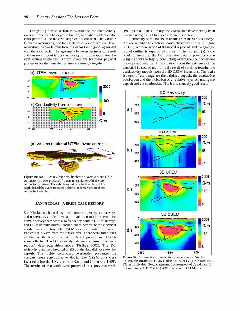
The geologic cross-section is overlaid on the conductivity inversion results. The depth to the top, and lateral extent of the main portion of the massive sulphide are outlined. The variable thickness overburden, and the existence of a more resistive layer separating the overburden from the deposit is in good agreement with the rock model. The agreement between the inversion result and the rock model is very encouraging. It also motivates the next section where results from inversions for many physical properties for the same deposit area are brought together.

Figure 49: (a) UTEM inversion results shown as a cross-section (b) a conductivity model produced from an interpolation of drill core conductivity testing. The solid lines indicate the boundary of the sulphide and the overburden (c) Volume rendered version of the conductivity model.

SAN NICOLAS - A BRIEF CASE HISTORY

San Nicolas has been the site of numerous geophysical surveys and it serves as an ideal test site. In addition to the UTEM time domain survey there were also frequency domain CSEM surveys and DC resistivity surveys carried out to determine the electrical conductivity structure. The CSEM survey consisted of a single transmitter 3.5 km from the survey area. There were three lines of data over the deposit area at which orthogonal E and H fields were collected. The DC resistivity data were acquired in a "real-section" data acquisition mode (Phillips 2002). The DC resistivity data were inverted in 3D but the data did not show the deposit. The highly conducting overburden prevented the currents from penetrating to depth. The CSEM data were inverted using the 1D algorithm (Routh and Oldenburg 1999). The results of that work were presented in a previous work

(Phillips et al. 2001). Finally, the CSEM data have recently been inverted using the 3D frequency domain inversion.

A summary of the inversion results from the various surveys that are sensitive to electrical conductivity are shown in Figure 50. Only a cross-section of the model is plotted, and the geologic model outline is superposed on each. The top plot (a) is the result of inverting the DC resistivity data. It provides some insight about the highly conducting overburden but otherwise conveys no meaningful information about the existence of the deposit. The second plot (b) is the result of stitching together the conductivity models from the 1D CSEM inversions. The main features of the image are the sulphide deposit, the conductive overburden and the indication of a resistive layer separating the deposit and the overburden. This is a reasonably good result.

Figure 50: Cross-section of conductivity models for San Nicolas deposit. Electrical conductivity models recovered by: (a) 3D inversion of DC resistivity data; (b) concatenating 1D inversions of CSEM data; (c) 3D inversion of UTEM data; (d) 3D inversions of CSEM data.


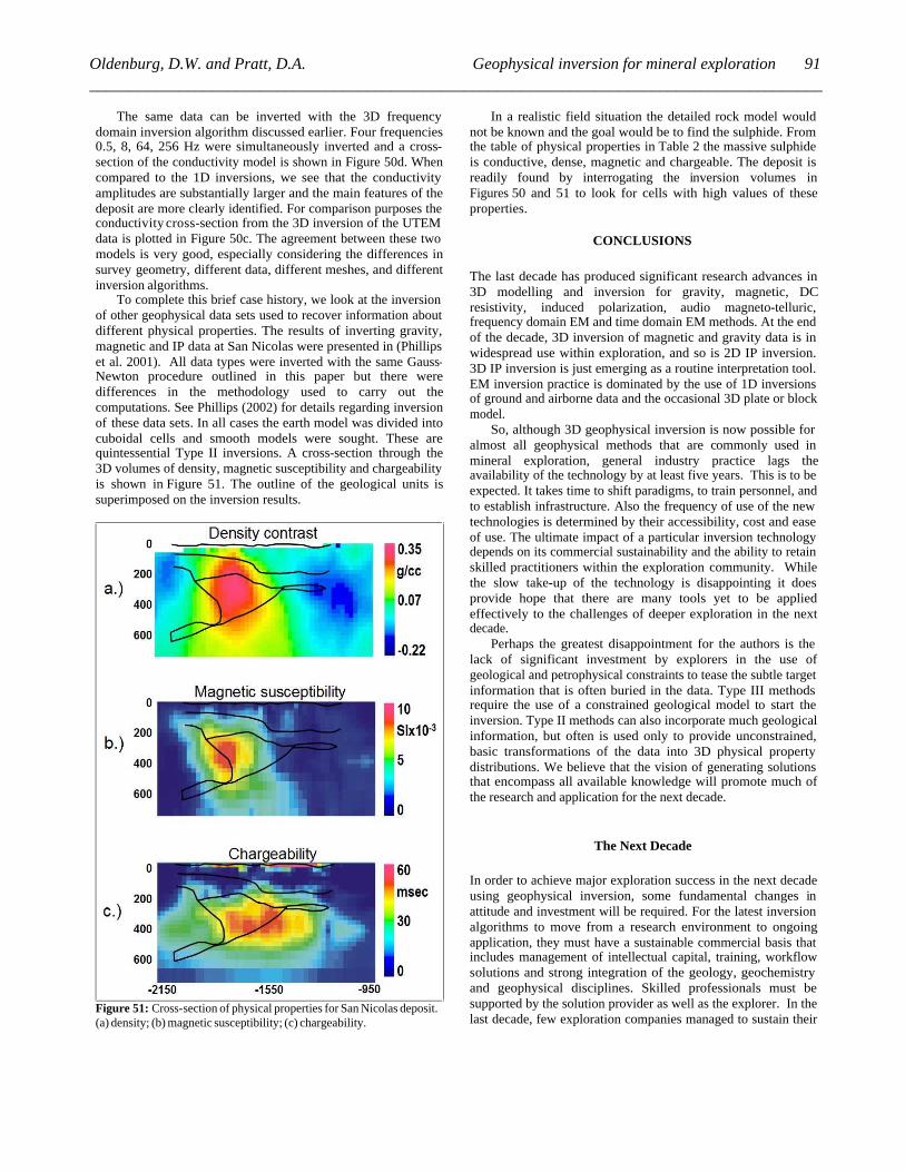
The same data can be inverted with the 3D frequency domain inversion algorithm discussed earlier. Four frequencies 0.5, 8, 64, 256 Hz were simultaneously inverted and a cross-section of the conductivity model is shown in Figure 50d. When compared to the 1D inversions, we see that the conductivity amplitudes are substantially larger and the main features of the deposit are more clearly identified. For comparison purposes the conductivity cross-section from the 3D inversion of the UTEM data is plotted in Figure 50c. The agreement between these two models is very good, especially considering the differences in survey geometry, different data, different meshes, and different inversion algorithms.

To complete this brief case history, we look at the inversion of other geophysical data sets used to recover information about different physical properties. The results of inverting gravity, magnetic and IP data at San Nicolas were presented in (Phillips et al. 2001). All data types were inverted with the same Gauss-Newton procedure outlined in this paper but there were differences in the methodology used to carry out the computations. See Phillips (2002) for details regarding inversion of these data sets. In all cases the earth model was divided into cuboidal cells and smooth models were sought. These are quintessential Type II inversions. A cross-section through the 3D volumes of density, magnetic susceptibility and chargeability is shown in Figure 51. The outline of the geological units is superimposed on the inversion results.

Figure 51: Cross-section of physical properties for San Nicolas deposit. (a) density; (b) magnetic susceptibility; (c) chargeability.

In a realistic field situation the detailed rock model would not be known and the goal would be to find the sulphide. From the table of physical properties in Table 2 the massive sulphide is conductive, dense, magnetic and chargeable. The deposit is readily found by interrogating the inversion volumes in Figures 50 and 51 to look for cells with high values of these properties.

CONCLUSIONS

The last decade has produced significant research advances in 3D modelling and inversion for gravity, magnetic, DC resistivity, induced polarization, audio magneto-telluric, frequency domain EM and time domain EM methods. At the end of the decade, 3D inversion of magnetic and gravity data is in widespread use within exploration, and so is 2D IP inversion. 3D IP inversion is just emerging as a routine interpretation tool. EM inversion practice is dominated by the use of 1D inversions of ground and airborne data and the occasional 3D plate or block model.

So, although 3D geophysical inversion is now possible for almost all geophysical methods that are commonly used in mineral exploration, general industry practice lags the availability of the technology by at least five years. This is to be expected. It takes time to shift paradigms, to train personnel, and to establish infrastructure. Also the frequency of use of the new technologies is determined by their accessibility, cost and ease of use. The ultimate impact of a particular inversion technology depends on its commercial sustainability and the ability to retain skilled practitioners within the exploration community. While the slow take-up of the technology is disappointing it does provide hope that there are many tools yet to be applied effectively to the challenges of deeper exploration in the next decade.

Perhaps the greatest disappointment for the authors is the lack of significant investment by explorers in the use of geological and petrophysical constraints to tease the subtle target information that is often buried in the data. Type III methods require the use of a constrained geological model to start the inversion. Type II methods can also incorporate much geological information, but often is used only to provide unconstrained, basic transformations of the data into 3D physical property distributions. We believe that the vision of generating solutions that encompass all available knowledge will promote much of the research and application for the next decade.

The Next Decade

In order to achieve major exploration success in the next decade using geophysical inversion, some fundamental changes in attitude and investment will be required. For the latest inversion algorithms to move from a research environment to ongoing application, they must have a sustainable commercial basis that includes management of intellectual capital, training, workflow solutions and strong integration of the geology, geochemistry and geophysical disciplines. Skilled professionals must be supported by the solution provider as well as the explorer. In the last decade, few exploration companies managed to sustain their


91

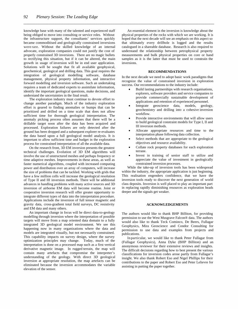
knowledge base with many of the talented and experienced staff being obliged to move into consulting or service roles. Without the infrastructure support, the consultants’ services quickly became commoditised and geologically constrained inversions were rare. Without the skilled knowledge of an internal advocate, exploration companies could not justify the cost of properly constrained 3D inversions. There are no magic bullets to rectifying this situation, but if it can be altered, the main growth in usage of inversion will be in end user application. Solutions will be sought that fit all available geophysical, geochemical, geological and drilling data. This goal requires the integration of geological modelling software, database management, physical property information, and interactive forward modelling and inversion software. Such an undertaking requires a team of dedicated experts to assimilate information, identify the important geological questions, make decisions, and understand the uncertainties in the final result.

The exploration industry must continue to devote effort to change another paradigm. Much of the industry exploration effort is geared to finding anomalies or bumps that can be prioritized and drilled on a time scale that does not allow sufficient time for thorough geological interpretation. The anomaly picking process often assumes that there will be a drillable target soon after the data has been acquired and processed. Exploration failures are only detected after the ground has been dropped and a subsequent explorer re-evaluates the data based upon a full geological model analysis. It is important to allow sufficient time and budget in the exploration process for constrained interpretation of all the available data.

On the research front, 3D EM inversion presents the greatest technical challenges. Evolution of 3D EM algorithms will involve the use of unstructured meshes and perhaps frequency or time adaptive meshes. Improvements in these areas, as well as faster numerical algorithms, coupled with increased computing power and distribution over an array of computers, will increase the size of problems that can be tackled. Working with grids that have a few million cells will increase the geological resolution of Type II and III inversion methods. There will be additional advances in handling problems with many active sources and 3D inversion of airborne EM data will become routine. Joint or cooperative inversion research will offer greater opportunity to integrate different types of data into the interpretation procedure. Applications include the inversion of full tensor magnetic and gravity data, cross-gradient total field surveys, DC resistivity and EM data and many others.

An important change in focus will be direct data-to-geology modelling through inversion where the interpretation of possible targets will move from a map oriented data domain to a fully integrated 3D geological model environment. We see this happening now in many organizations where the data and models are integrated visually, but not necessarily constrained. This capability impacts on survey design, where the survey optimization principles may change. Today, much of the interpretation is done on a processed map such as a first vertical derivative magnetic image. In rugged terrain, the map will contain many artefacts that compromise the interpreter’s understanding of the geology. With direct 3D geological inversion at appropriate resolution, the map artefacts can be eliminated because the inversion accommodates the variable elevation of the sensor.

An essential element in the inversion is knowledge about the physical properties of the rocks with which we are working. It is hoped that the next decade will see an emphasis on this aspect so that ultimately every drillhole is logged and the results catalogued in a shareable database. Research is also required to understand the relationship between petrophysical property measurements and bulk physical properties on core or hand samples as it is the latter that must be used to constrain the inversions.

RECOMMENDATIONS

In the next decade we need to adopt basic work paradigms that recognize the value of constrained inversion in exploration success. Our recommendations to the industry include:

· Build lasting partnerships with research organisations, explorers, software providers and service companies to provide commercially sustainable development of applications and retention of experienced personnel.

· Integrate geoscience data, models, geology, geochemistry and drilling into a cohesive inversion workflow.

· Provide interactive environments that will allow users to build geological constraint models for Type I, II and III inversion methods.

· Allocate appropriate resources and time to the interpretation phase following data collection.

· Select methods that are appropriate to the geological objectives and resource availability.

· Collate rock property databases for each exploration terrane.

· Invest in training of senior staff to utilize and appreciate the value of investment in geologically constrained inversion processes.

While the take-up of inversion tools has been widespread within the industry, the appropriate application is just beginning. This realisation engenders confidence, that we have the inversion tools ready to discover the next generation of world class deposits. Inversion is well placed to play an important part in replacing rapidly diminishing resources as exploration heads deeper and the signals get weaker.

ACKNOWLEDGEMENTS

The authors would like to thank BHP Billiton, for providing permission to use the West Musgrave Falcon® data. The authors would also like to thank Teck Cominco, De Beers, Fullagar Geophysics, Mira Geoscience and Condor Consulting for permission to use data and examples from projects and publications.

In particular, we would like to thank Peter Fullagar from (Fullagar Geophysics), Anna Dyke (BHP Billiton) and an anonymous reviewer for their extensive reviews and insights. The difficult decisions regarding how to best present the various classifications for inversion codes arose partly from Fullagar’s insight. We also thank Robert Eso and Nigel Phillips for their contributions to the paper and Robert Eso and Peter Lelievre for assisting in putting the paper together.


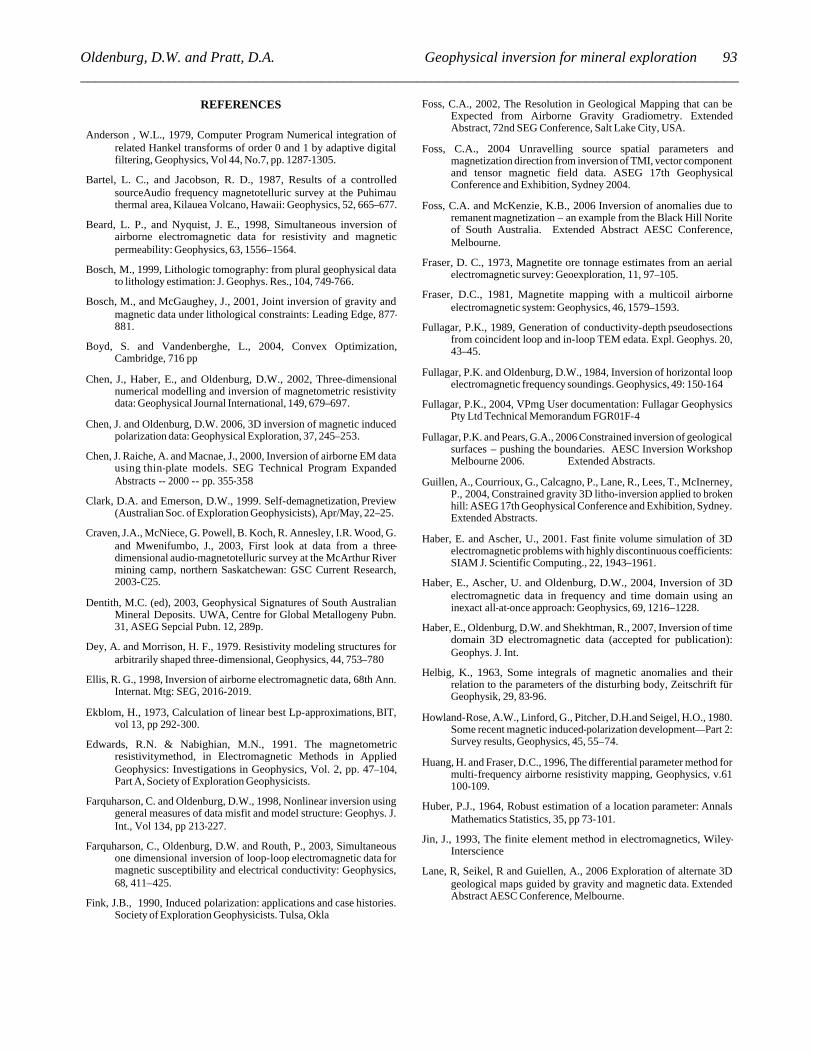
REFERENCES

Anderson , W.L., 1979, Computer Program Numerical integration of

related Hankel transforms of order 0 and 1 by adaptive digital filtering, Geophysics, Vol 44, No.7, pp. 1287-1305.

Bartel, L. C., and Jacobson, R. D., 1987, Results of a controlled sourceAudio frequency magnetotelluric survey at the Puhimau thermal area, Kilauea Volcano, Hawaii: Geophysics, 52, 665–677.

Beard, L. P., and Nyquist, J. E., 1998, Simultaneous inversion of airborne electromagnetic data for resistivity and magnetic permeability: Geophysics, 63, 1556–1564.

Bosch, M., 1999, Lithologic tomography: from plural geophysical data to lithology estimation: J. Geophys. Res., 104, 749-766.

Bosch, M., and McGaughey, J., 2001, Joint inversion of gravity and magnetic data under lithological constraints: Leading Edge, 877-881.

Boyd, S. and Vandenberghe, L., 2004, Convex Optimization, Cambridge, 716 pp

Chen, J., Haber, E., and Oldenburg, D.W., 2002, Three-dimensional numerical modelling and inversion of magnetometric resistivity data: Geophysical Journal International, 149, 679–697.

Chen, J. and Oldenburg, D.W. 2006, 3D inversion of magnetic induced polarization data: Geophysical Exploration, 37, 245–253.

Chen, J. Raiche, A. and Macnae, J., 2000, Inversion of airborne EM data using thin-plate models. SEG Technical Program Expanded Abstracts -- 2000 -- pp. 355-358

Clark, D.A. and Emerson, D.W., 1999. Self-demagnetization, Preview (Australian Soc. of Exploration Geophysicists), Apr/May, 22–25.

Craven, J.A., McNiece, G. Powell, B. Koch, R. Annesley, I.R. Wood, G. and Mwenifumbo, J., 2003, First look at data from a three-dimensional audio-magnetotelluric survey at the McArthur River mining camp, northern Saskatchewan: GSC Current Research, 2003-C25.

Dentith, M.C. (ed), 2003, Geophysical Signatures of South Australian Mineral Deposits. UWA, Centre for Global Metallogeny Pubn. 31, ASEG Sepcial Pubn. 12, 289p.

Dey, A. and Morrison, H. F., 1979. Resistivity modeling structures for arbitrarily shaped three-dimensional, Geophysics, 44, 753–780

Ellis, R. G., 1998, Inversion of airborne electromagnetic data, 68th Ann. Internat. Mtg: SEG, 2016-2019.

Ekblom, H., 1973, Calculation of linear best Lp-approximations, BIT, vol 13, pp 292-300.

Edwards, R.N. & Nabighian, M.N., 1991. The magnetometric resistivitymethod, in Electromagnetic Methods in Applied Geophysics: Investigations in Geophysics, Vol. 2, pp. 47–104, Part A, Society of Exploration Geophysicists.

Farquharson, C. and Oldenburg, D.W., 1998, Nonlinear inversion using general measures of data misfit and model structure: Geophys. J. Int., Vol 134, pp 213-227.

Farquharson, C., Oldenburg, D.W. and Routh, P., 2003, Simultaneous one dimensional inversion of loop-loop electromagnetic data for magnetic susceptibility and electrical conductivity: Geophysics, 68, 411–425.

Fink, J.B., 1990, Induced polarization: applications and case histories. Society of Exploration Geophysicists. Tulsa, Okla

Foss, C.A., 2002, The Resolution in Geological Mapping that can be Expected from Airborne Gravity Gradiometry. Extended Abstract, 72nd SEG Conference, Salt Lake City, USA.

Foss, C.A., 2004 Unravelling source spatial parameters and magnetization direction from inversion of TMI, vector component and tensor magnetic field data. ASEG 17th Geophysical Conference and Exhibition, Sydney 2004.

Foss, C.A. and McKenzie, K.B., 2006 Inversion of anomalies due to remanent magnetization – an example from the Black Hill Norite of South Australia. Extended Abstract AESC Conference, Melbourne.

Fraser, D. C., 1973, Magnetite ore tonnage estimates from an aerial electromagnetic survey: Geoexploration, 11, 97–105.

Fraser, D.C., 1981, Magnetite mapping with a multicoil airborne electromagnetic system: Geophysics, 46, 1579–1593.

Fullagar, P.K., 1989, Generation of conductivity-depth pseudosections from coincident loop and in-loop TEM edata. Expl. Geophys. 20, 43–45.

Fullagar, P.K. and Oldenburg, D.W., 1984, Inversion of horizontal loop electromagnetic frequency soundings. Geophysics, 49: 150-164

Fullagar, P.K., 2004, VPmg User documentation: Fullagar Geophysics Pty Ltd Technical Memorandum FGR01F-4

Fullagar, P.K. and Pears, G.A., 2006 Constrained inversion of geological surfaces – pushing the boundaries. AESC Inversion Workshop Melbourne 2006. Extended Abstracts.

Guillen, A., Courrioux, G., Calcagno, P., Lane, R., Lees, T., McInerney, P., 2004, Constrained gravity 3D litho-inversion applied to broken hill: ASEG 17th Geophysical Conference and Exhibition, Sydney. Extended Abstracts.

Haber, E. and Ascher, U., 2001. Fast finite volume simulation of 3D electromagnetic problems with highly discontinuous coefficients: SIAM J. Scientific Computing., 22, 1943–1961.

Haber, E., Ascher, U. and Oldenburg, D.W., 2004, Inversion of 3D electromagnetic data in frequency and time domain using an inexact all-at-once approach: Geophysics, 69, 1216–1228.

Haber, E., Oldenburg, D.W. and Shekhtman, R., 2007, Inversion of time domain 3D electromagnetic data (accepted for publication): Geophys. J. Int.

Helbig, K., 1963, Some integrals of magnetic anomalies and their relation to the parameters of the disturbing body, Zeitschrift für Geophysik, 29, 83-96.

Howland-Rose, A.W., Linford, G., Pitcher, D.H.and Seigel, H.O., 1980. Some recent magnetic induced-polarization development—Part 2: Survey results, Geophysics, 45, 55–74.

Huang, H. and Fraser, D.C., 1996, The differential parameter method for multi-frequency airborne resistivity mapping, Geophysics, v.61 100-109.

Huber, P.J., 1964, Robust estimation of a location parameter: Annals Mathematics Statistics, 35, pp 73-101.

Jin, J., 1993, The finite element method in electromagnetics, Wiley-Interscience

Lane, R, Seikel, R and Guiellen, A., 2006 Exploration of alternate 3D geological maps guided by gravity and magnetic data. Extended Abstract AESC Conference, Melbourne.


93

Lee, T.J., 1980, Rapid computation of magnetic anomalies with demagnetisation included for arbitrarily shaped magnetic bodies. Geophysical Jour. Royal Astronomical Soc., 60, 67-75.

Lelievre, P.G., Oldenburg, D.W. and Phillips, N., 2006, 3D magnetic inversion for total magnetization in areas with complicated remanence. SEG/New Orleans 2006 Annual Meeting.

Li, Y. and Oldenburg, D.W., 1995, 3D inversion of gravity data. SEG Technical Program Expanded Abstracts – 1995, 264-267

Li, Y., and Oldenburg, D.W., 1996, 3D inversion of magnetic data: Geophysics, 61, 394–408.

Li, Y., and Oldenburg D.W., 1997, 3D inversion of DC resisitivyt and IP data; extended abstract Exploration 97

Li, Y. and Oldenburg, D.W., 2000, 3D inversion of induced polarization data: Geophysics, 65, 1931–1945.

Li, Y. and Oldenburg, D.W., 2003, Fast inversion of large-scale magnetic data using wavelet transforms and logarithmic barrier method: Geophys. J. Int, 152, 251–265.

Li, Y., Shearer, S., Haney, M. and Dannemiller, N., 2004 Comprehensive approaches to the inversion of magnetic data with strong remanent magnetization. SEG Int'l Exposition and 74th Annual Meeting Denver, Colorado 10-15 October 2004.

Loke, M.H. and Dahlin, T., (1997) A combined Gauss-Newton and quasi-Newton inversion method for the inversion of apparent resistivity pseudosections, Procs. 3rd Meeting Environmental and Engineering Geophysics, Aarhus, Denmark, 8-11 September 1997, p 139-142.

Macnae, J.C., King, A., Stolz, E.M., 1998 Fast AEM data processing and inversion. Exploration Geophysics, v.29, No. 1 – 2 pp.163-169.

Marquis, R., B. D. and McGaughey, J., 2003, Quantitative geology using 3D common-earth modeling: PDAC extended abstract.

Morris, W.A.. Ugalde, H. and Thomson, V., 2007 Magnetic Remanence Mapping: Some Do’s and Some Don’ts!, KEGS PDAC Inversion Symposium.

Mutton, A. J., 1997, The application of geophysics during evaluation of the Century zinc deposit: 4th Decennial Internat. Conf. Min. Expl., Proceedings, 599–614.

Nocedal, J. and Wright, S.J., 1999, Numerical Optimization, Springer Series in Operations Research, Springer, .636 pp.

Napier, S., 2007, Practical inversion of 3D time domain electromagnetic data, MSc thesis, University of British Columbia.

Oldenburg, D.W. and Li, Y., 1994, Inversion of induced polarization data: Geophysics, 59, 1327–1341.

Oldenburg, D.W., Li, Y., Farquharson, C., Kowalczyk, P., Aravanis, T., King, A., and Watts, A., 1998, Applications of geophysical inversions in mineral exploration problems: The Leading Edge, 17, 461–465.

Oldenburg, D., Shehktman, R., Eso, R., Farquharson, C.G., Eaton, P., Anderson, B., Bolin, B., 2004, Closing the gap between research and practice in EM data interpretation. SEG Technical Program Expanded Abstracts, 2004. pp. 1179-1182.

Oldenburg, D. W., Eso, R., Napier, S. and Haber, E., 2005, Controlled source electromagnetic inversion for resource exploration: First Break, 23, 41–48.

Oldenburg, D.W. and Li, Y., 2005, Inversion for applied geophyscis: a tutorial. N e a r -surface geophysics, SEG investigations in geophysics series No 13, editor Dwain Butler, pp 89–150.

Oristaglio M., and Spies, B., 1999, Three-dimensional electromagnetics, Geophysical Developments No. 7, SEG Geophysical Development Series, Michael R. Cooper editor.

Phillips, N., 2002, Geophysical inversion in an integrated exploration program: examples from the San Nicolas deposit, MSc thesis, University of British Columbia

Phillips, N., Oldenburg, D.W. Chen, J. Li, L. and Routh, P., 2001, Cost effectiveness of geophysical inversion in mineral exploration: applications at San Nicolas.: The Leading Edge, 20, pp1351–1350.

Pratt, D.A., McKenzie, K.B., White, A.S., Foss, C.A., Shamin, A. and Shi, Z., 2001 A user guided expert system approach to 3D interpretation of magnetic anomalies. Extended Abstracts, ASEG 15th Geophysical Conference and Exhibition, Brisbane.

Pratt, D.A., Foss, C.A., Shi, Z, White,A.S., McKenzie, K.B, Gidley, P.R. and Mann,S., 2007, Encom ModelVision Pro, Encom AutoMag - the 3D workbench for magnetic and gravity interpretation, Reference Manual. Encom Technology, 504 p.

Pratt,D.A., Foss, C.A. and Roberts, S., 2006 User Guided Inversion & Visualisation of Interpretation Confidence. Extended Abstract AESC Conference, Melbourne.

Raiche, A., Wilson, G., and Sugeng, F., 2006, Practical 3D AEM inversion using thin-sheet models: Extended Abstracts, Australian Earth Science Convention, Melbourne VIC.

Rajagopalan, S., Schmidt, P.W. and Clark, D.A., 1993, Rock magnetism and geophysical interpretation of the Black Hill Norite, South Australia, Exploration Geophysics, 24, 209- 212.

Routh, P. and Oldenburg, D.W., 1999, Inversion of controlled source audio-frequency magnetotelluric data for a horizontally layered earth: Geophysics, 64, 1689–1697.

Saad,Y., 1996, Iterative methods for sparse linear systems, PWS Publishing, pp 447.

Schmidt, P.W., and Clark, D.A., 1998, The calculation of magnetic components and moments from TMI: A case study from the Tuckers igneous complex, Queensland, Exploration Geophysics, 29, 609-614.

Seigel, H.O., 1974, The magnetic induced polarization method: Geophysics, 39, 321–339.

Seigel, H.O., and Howland-Rose, A.W., 1990, Magnetic induced-polarization method: in Fink, J.B., Sternberg, B.K., McAlister, E.O., and Wieduwilt, W.G. (eds) , Induced polarization:Applications and case histories, Investigations in Geophysics, vol. 4, Society of Exploration Geophysicists, 23–56.

Siripunvaraporn W., Egbert, G. and Uyeshima, M., 2005, Interpretation of 2-D Magnetotelluric Profile Data with 3-D Inversion: Synthetic Examples, Geophys. Jour. Inter. , 160, 804-814.

Siripunvaraporn, W., Egbert, G., Lenbury, Y. and Uyeshima, M., 2005, Three-dimensional magnetotelluric inversion: data-space method: Physics of the Earth and Planetary Interiors, 150, 3–14.

Stolz, R., Zakosarenko, V., Schulz, M., Chwala, A., Fritzsch, L. Meyer, H.-G. and Köstlin, E. O., 2006, Magnetic full-tensor SQUID gradiometer system for geophysical applications


The Leading Edge, Volume 25, Issue 2, pp. 178-180.

Stolz, E.M. and Macnae, J., 1998, Evaluating EM waveforms by singular-value decomposition of exponential basis functions: Geophysics 63, 64-74)

Tikhonov, A.V., and Arsenin, V.Y., 1977, Solution of ill-posed problems: John Wiley and Sons, Inc.

Tuncer, V., Unsworth, M.J, Siripunvaraporn, W. and Craven, J.A., 2006, Audio-magnetotelluric exploration for unconformity uranium deposits in the Athabasca Basin, Saskatachewan, Canada. Extended Abstract, SEG/New Orleans 2006 Annual Meeting.

Unsworth, M. Tuncer, V., Siripunvaraporn, W. and Craven, J., 2006, Exploration for unconformity uranium deposits with audiomagnetotellurics. MS Power Point presentation, SEG/New Orleans 2006 Annual Meeting.

Vogel, C. R., 2001, Computational methods for inverse problems: Society of Industrial and Applied Mathematics, Frontiers in Applied Mathematics.

Wilson, G.A., R. A. and Sugeng, F., 2006, 2.5D inversion of airborne electromagnetic data: Extended Abstracts, AESC Conference, Melbourne 2006..

Witherly, K., 2005 VTEM Survey over the Wheatley project area Bridgetown, Western Australia Report (unpub.) for Teck Cominco Australia Pty. Ltd. February, 2005 Condor Consulting, Inc., Project 476

Witherly, K. 2006 Manjimup AEM Test Site. Report (unpub.) by Condor Consulting for Teck Cominco 13p.

Yee, K.S., 1966, Numerical solution of initial boundary value problems involving Maxwell’s equations in isotropic media: IEEE, AP-14, pp 302-307.

Zhang, Z. and D.W. Oldenburg, 1999, Simultaneous reconstruction of 1D susceptibility and conductivity from em data: Geophysics, 64, 33–47.

Zhdanov, M.S. , 2007, New advances in regularized inversion and imaging of gravity, magnetic and electromagnetic data. Extended Abstract for EGM International Workshop, Capri, Italy.

Zhdanov, M.S., Ellis, R., and Mukherje, S., 2004 Three-dimensional regularized focusing inversion of gravity gradient tensor component data. Geoph., v.69, (4), p. 925–937.

Zonge, K.L., Wynn, J., and Urquhart, S., 2005, Resistivity, induced polarization, and complex resistivity, Near-surface geophysics, SEG investigations in geophysics series No 13, editor Dwain Butler, pp 265–300.

Zonge, K. L., and Hughes, L. J., 1991, Controlled source audiofrequency magnetotellurics, in Nabighian, M. N., Ed., Electromagnetic methods in applied geophysics, 2: Soc. Expl. Geophysics.


95

Documents

Geophysical Inversion for Mineral Exploration: a … · Geophysical Inversion for Mineral Exploration: ... mining house. The latter has since ... method depends upon existing geological