Geophysical Journal InternationalGeophys. J. Int. (2016) 206, 1645–1651 doi: 10.1093/gji/ggw236Advance Access publication 2016 June 29GJI Seismology

Structure of the Los Angeles Basin from ambient noiseand receiver functions

Yiran Ma and Robert W. ClaytonSeismological Laboratory, California Institute of Technology, Pasadena, CA 91125, USA. E-mail: yrma@caltech.edu

Accepted 2016 June 20. Received 2016 June 18; in original form 2016 March 29

S U M M A R YA velocity (Vs) and structure model is derived for the Los Angeles Basin, California basedon ambient-noise surface wave and receiver-function analysis, using data from a low-cost,short-duration, dense broad-band survey (LASSIE) deployed across the basin. The shear wavevelocities show lateral variations at the Compton-Los Alamitos and the Whittier Faults. Thebasement beneath the Puente Hills–San Gabriel Valley shows an unusually high velocity(∼4.0 km s−1) and indicates the presence of schist. The structure of the model shows that thebasin is a maximum of 8 km deep along the profile and that the Moho rises to a depth of 17 kmunder the basin. The basin has a stretch factor of 2.6 in the centre grading to 1.3 at the edgesand is in approximate isostatic equilibrium.

Key words: Interferometry; Interface waves; Seismic tomography.

1 I N T RO D U C T I O N

The Los Angeles Basin is a Miocene-age pull-apart basin that wasformed by the passing of the Pacific-Juan de Fuca-North Amer-ica triple junction by southern California (Nicholson et al. 1994;Ingersoll & Rumelhart 1999). Ingersoll & Rumelhart (1999) haveproposed a three-stage model for its evolution, including transro-tation (18–12 Ma), transtension (12–6 Ma) and transpression (6–0Ma) episodes. The LA Basin has been extensively studied overthe last few decades because it is a significant oil-production area(Wright 1991), and because it is a major concern for the seismichazard evaluation for the area (Olsen 2000; Komatitsch et al. 2004).The basin is part of the seismic hazard because the sediments trapand amplify strong motion energy, and because of its size and depth,the basin is capable of enhancing waves in the 2–5 s range, whichis particularly dangerous for the high-rise buildings in the area. Nu-merical modeling of these phenomena requires an accurate model ofthe subsurface structure and velocities that define the Los AngelesBasin.

An initial unified model for the southern California region wasproduced by Magistrale et al. (2000) with a mixture of variousstudies such as receiver functions (RFs; Zhu & Kanamori 2000)and tomography (Hauksson 2000). The basin structure was basedon empirical rules applied to formation maps that were interpolatedfrom borehole data. Another approach was used in Suss & Shaw(2003), where they used P-wave velocity measurements determinedfrom stacking velocities from oil-company reflection surveys andsonic logs from boreholes, along with a basin shape model basedon gravity and borehole lithology observations (McCulloh 1960;Yerkes et al. 1965). These models have been combined and further

enhanced through the use of full waveform inversions (Tape et al.2009; Lee et al. 2014), leading to an updated unified model (Shawet al. 2015) including the CVM-H velocity model (currently 15.1.0version) and the CFM fault model. Fig. S1 in the Supporting In-formation shows the CVM-H model beneath the array. The shallowstructure (less than 10 km depth) shows significant lateral variation,while the deeper part is almost constant except for a slight dip onthe Moho.

In this paper, we add some additional constraints on the structureof the Los Angeles Basin and its shear wave velocities. This study isbased on a new survey that was done in the fall of 2014. It consistedof a relatively dense array of broad-band sensors that traversed thebasin from Long Beach, through Whittier to the southern part ofthe San Gabriel Valley. Fig. 1 shows the location of the experiment,which is named ‘Los Angeles Syncline Seismic Interferometry Ex-periment’ (LASSIE). It includes 73 three-component broad-bandstations, 51 of which are deployed in a line with ∼1 km interstationdistance. They were operational from 2014 September to Novem-ber, with average recording time of about 40 d. This survey is anexample of what can be done with a low-cost, short-duration, rapid-deployment style that may prove useful for conducting additionalsurveys to refine the basin model.

We use ambient-noise-derived surface waves and RFs to constructthe new model. Both are traditionally thought of as not being veryuseful in an urban environment where the cultural noise can beoverwhelming, and the basin reverberations can make it difficult toidentify the various phases in the RFs. However, as shown here, anexcellent signal can be obtained and the key is to have a dense arrayto use lateral continuity to distinguish the interface signals from thenoise.

C© The Authors 2016. Published by Oxford University Press on behalf of The Royal Astronomical Society. 1645

at California Institute of T

echnology on July 22, 2016http://gji.oxfordjournals.org/

Dow

nloaded from

1646 Y. Ma and R.W. Clayton

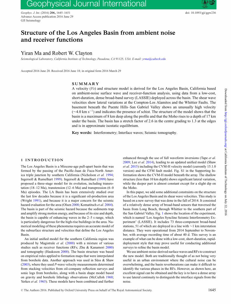
Figure 1. The LASSIE array. The yellow and red dots are LASSIE stations, and the black circles are SCSN stations. The green line denotes the location of the2-D profile (A–A′), and the distances from A are marked with blue crosses in 10 km intervals. The faults are shown in pink lines (Jennings & Bryant 2010).LA: Los Angeles, LAB: Los Angeles Basin, SGV: San Gabriel Valley, NIF: Newport-Inglewood Fault, C-LAF: Compton-Los Alamitos Fault, WF: WhittierFault. The Ps conversion points at 20 km depth are plotted for the two events used in the receiver functions (Fig. 2).

Table 1. Events with clear recordings. The top two events happened during most stations were in operation, andare used in the receiver-function analysis.

Time∗ Latitude (◦) Longitude (◦) Depth (km) Magnitude Backazimuth (◦) Distance (◦)

20141009021431 –32.1082 –110.811 16.54 7 173.231 66.007620141014035134 12.5262 –88.1225 40 7.3 120.746 34.591720140924111615 –23.8009 –66.6321 224 6.2 132.236 75.410920141101185722 –19.6903 –177.759 434 7.1 236.282 77.8924∗Time is in the format of YYYYMMDDHHMMSS.

2 R E C E I V E R F U N C T I O N S

Standard methods are used to retrieve and process the RFs (Ma& Clayton 2015). For each seismic event, the data are rotated toR-T-Z coordinates and filtered to a 1–50 s passband. An iterativetime-domain deconvolution (Ligorrıa & Ammon 1999) is used toretrieve the P-to-S RFs. A low-pass Gaussian filter is applied with aparameter of 2.5, which means the corresponding cut-off frequencyis ∼1.2 Hz and the pulse width in time domain is ∼1.0 s (see theSupporting Information). The events we used are within a 30◦–95◦ epicentral distance, and have magnitude no less than 6. Twoevents (Table 1) with clear recordings occurred while most stationswere in operation, and are used in the following processing. Theirapproximate Ps conversion points at 20 km depth are shown inFig. 1.

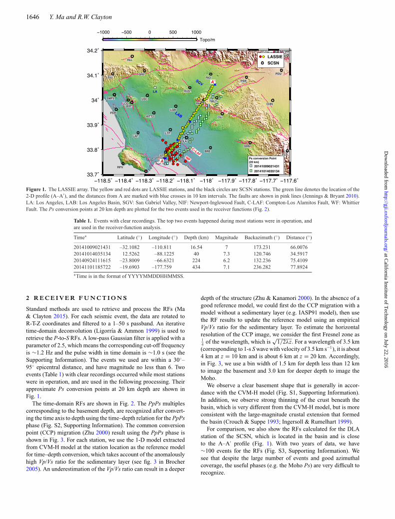
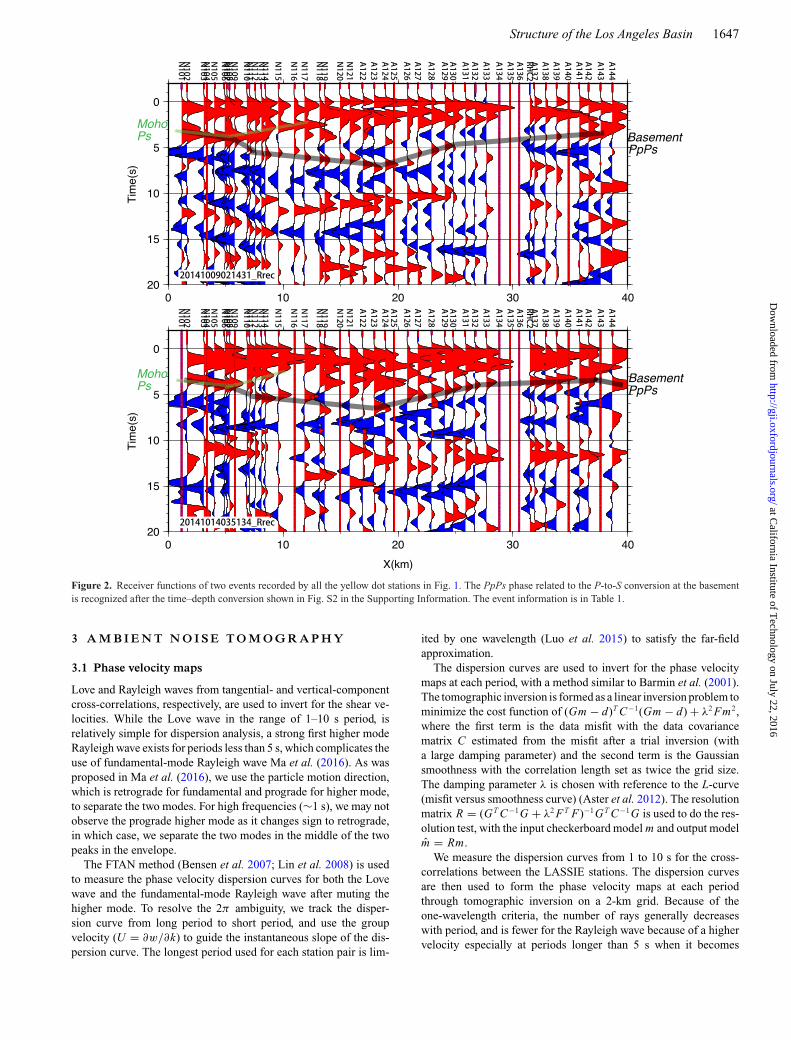
The time-domain RFs are shown in Fig. 2. The PpPs multiplescorresponding to the basement depth, are recognized after convert-ing the time axis to depth using the time–depth relation for the PpPsphase (Fig. S2, Supporting Information). The common conversionpoint (CCP) migration (Zhu 2000) result using the PpPs phase isshown in Fig. 3. For each station, we use the 1-D model extractedfrom CVM-H model at the station location as the reference modelfor time–depth conversion, which takes account of the anomalouslyhigh Vp/Vs ratio for the sedimentary layer (see fig. 3 in Brocher2005). An underestimation of the Vp/Vs ratio can result in a deeper

depth of the structure (Zhu & Kanamori 2000). In the absence of agood reference model, we could first do the CCP migration with amodel without a sedimentary layer (e.g. IASP91 model), then usethe RF results to update the reference model using an empiricalVp/Vs ratio for the sedimentary layer. To estimate the horizontalresolution of the CCP image, we consider the first Fresnel zone as14 of the wavelength, which is

√1/2λz. For a wavelength of 3.5 km

(corresponding to 1-s S wave with velocity of 3.5 km s−1), it is about4 km at z = 10 km and is about 6 km at z = 20 km. Accordingly,in Fig. 3, we use a bin width of 1.5 km for depth less than 12 kmto image the basement and 3.0 km for deeper depth to image theMoho.

We observe a clear basement shape that is generally in accor-dance with the CVM-H model (Fig. S1, Supporting Information).In addition, we observe strong thinning of the crust beneath thebasin, which is very different from the CVM-H model, but is moreconsistent with the large-magnitude crustal extension that formedthe basin (Crouch & Suppe 1993; Ingersoll & Rumelhart 1999).

For comparison, we also show the RFs calculated for the DLAstation of the SCSN, which is located in the basin and is closeto the A–A′ profile (Fig. 1). With two years of data, we have∼100 events for the RFs (Fig. S3, Supporting Information). Wesee that despite the large number of events and good azimuthalcoverage, the useful phases (e.g. the Moho Ps) are very difficult torecognize.

at California Institute of T

echnology on July 22, 2016http://gji.oxfordjournals.org/

Dow

nloaded from

Structure of the Los Angeles Basin 1647

Figure 2. Receiver functions of two events recorded by all the yellow dot stations in Fig. 1. The PpPs phase related to the P-to-S conversion at the basementis recognized after the time–depth conversion shown in Fig. S2 in the Supporting Information. The event information is in Table 1.

3 A M B I E N T N O I S E T O M O G R A P H Y

3.1 Phase velocity maps

Love and Rayleigh waves from tangential- and vertical-componentcross-correlations, respectively, are used to invert for the shear ve-locities. While the Love wave in the range of 1–10 s period, isrelatively simple for dispersion analysis, a strong first higher modeRayleigh wave exists for periods less than 5 s, which complicates theuse of fundamental-mode Rayleigh wave Ma et al. (2016). As wasproposed in Ma et al. (2016), we use the particle motion direction,which is retrograde for fundamental and prograde for higher mode,to separate the two modes. For high frequencies (∼1 s), we may notobserve the prograde higher mode as it changes sign to retrograde,in which case, we separate the two modes in the middle of the twopeaks in the envelope.

The FTAN method (Bensen et al. 2007; Lin et al. 2008) is usedto measure the phase velocity dispersion curves for both the Lovewave and the fundamental-mode Rayleigh wave after muting thehigher mode. To resolve the 2π ambiguity, we track the disper-sion curve from long period to short period, and use the groupvelocity (U = ∂w/∂k) to guide the instantaneous slope of the dis-persion curve. The longest period used for each station pair is lim-

ited by one wavelength (Luo et al. 2015) to satisfy the far-fieldapproximation.

The dispersion curves are used to invert for the phase velocitymaps at each period, with a method similar to Barmin et al. (2001).The tomographic inversion is formed as a linear inversion problem tominimize the cost function of (Gm − d)T C−1(Gm − d) + λ2 Fm2,where the first term is the data misfit with the data covariancematrix C estimated from the misfit after a trial inversion (witha large damping parameter) and the second term is the Gaussiansmoothness with the correlation length set as twice the grid size.The damping parameter λ is chosen with reference to the L-curve(misfit versus smoothness curve) (Aster et al. 2012). The resolutionmatrix R = (GT C−1G + λ2 F T F)−1GT C−1G is used to do the res-olution test, with the input checkerboard model m and output modelm = Rm.

We measure the dispersion curves from 1 to 10 s for the cross-correlations between the LASSIE stations. The dispersion curvesare then used to form the phase velocity maps at each periodthrough tomographic inversion on a 2-km grid. Because of theone-wavelength criteria, the number of rays generally decreaseswith period, and is fewer for the Rayleigh wave because of a highervelocity especially at periods longer than 5 s when it becomes

at California Institute of T

echnology on July 22, 2016http://gji.oxfordjournals.org/

Dow

nloaded from

1648 Y. Ma and R.W. Clayton

Figure 3. CCP migration with PpPs phase. The white lines delineate theinferred basement and Moho depths.

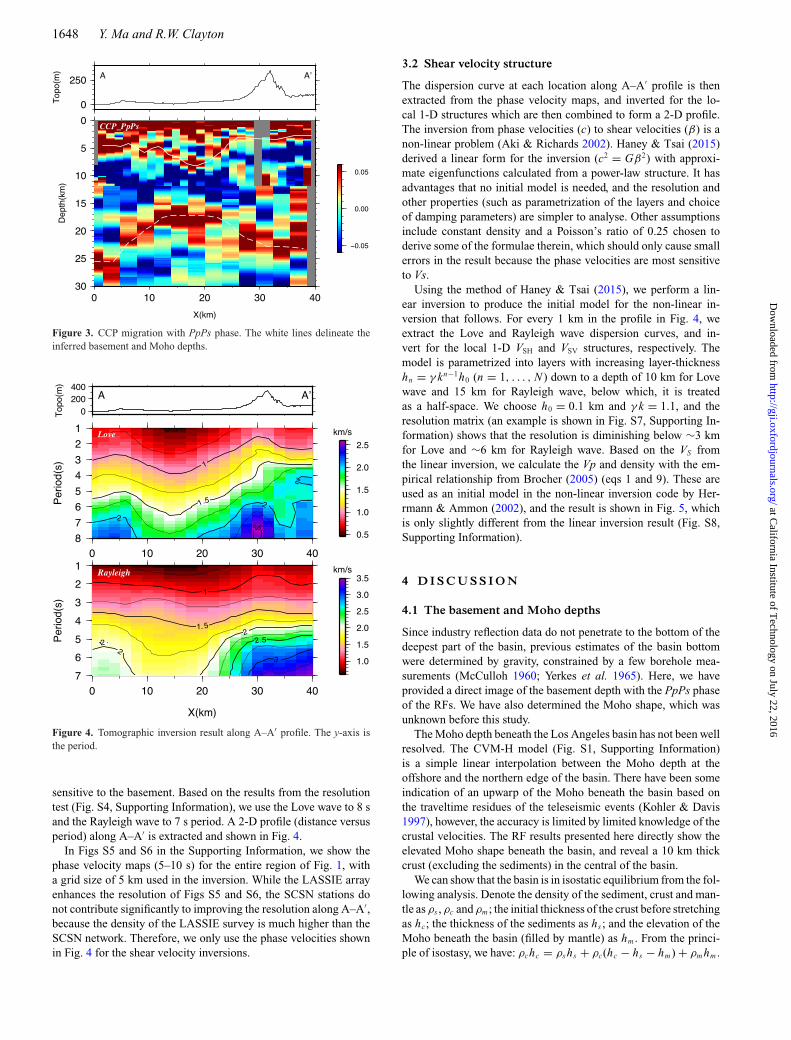
Figure 4. Tomographic inversion result along A–A′ profile. The y-axis isthe period.

sensitive to the basement. Based on the results from the resolutiontest (Fig. S4, Supporting Information), we use the Love wave to 8 sand the Rayleigh wave to 7 s period. A 2-D profile (distance versusperiod) along A–A′ is extracted and shown in Fig. 4.

In Figs S5 and S6 in the Supporting Information, we show thephase velocity maps (5–10 s) for the entire region of Fig. 1, witha grid size of 5 km used in the inversion. While the LASSIE arrayenhances the resolution of Figs S5 and S6, the SCSN stations donot contribute significantly to improving the resolution along A–A′,because the density of the LASSIE survey is much higher than theSCSN network. Therefore, we only use the phase velocities shownin Fig. 4 for the shear velocity inversions.

3.2 Shear velocity structure

The dispersion curve at each location along A–A′ profile is thenextracted from the phase velocity maps, and inverted for the lo-cal 1-D structures which are then combined to form a 2-D profile.The inversion from phase velocities (c) to shear velocities (β) is anon-linear problem (Aki & Richards 2002). Haney & Tsai (2015)derived a linear form for the inversion (c2 = Gβ2) with approxi-mate eigenfunctions calculated from a power-law structure. It hasadvantages that no initial model is needed, and the resolution andother properties (such as parametrization of the layers and choiceof damping parameters) are simpler to analyse. Other assumptionsinclude constant density and a Poisson’s ratio of 0.25 chosen toderive some of the formulae therein, which should only cause smallerrors in the result because the phase velocities are most sensitiveto Vs.

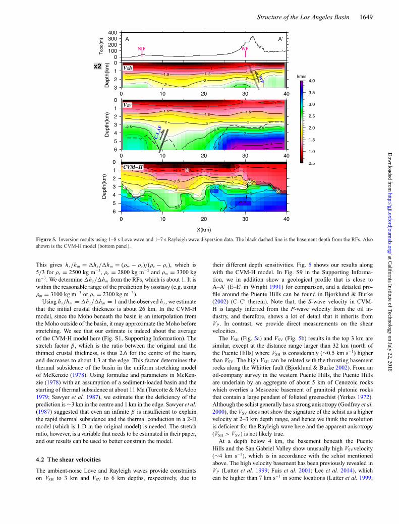
Using the method of Haney & Tsai (2015), we perform a lin-ear inversion to produce the initial model for the non-linear in-version that follows. For every 1 km in the profile in Fig. 4, weextract the Love and Rayleigh wave dispersion curves, and in-vert for the local 1-D VSH and VSV structures, respectively. Themodel is parametrized into layers with increasing layer-thicknesshn = γ kn−1h0 (n = 1, . . . , N ) down to a depth of 10 km for Lovewave and 15 km for Rayleigh wave, below which, it is treatedas a half-space. We choose h0 = 0.1 km and γ k = 1.1, and theresolution matrix (an example is shown in Fig. S7, Supporting In-formation) shows that the resolution is diminishing below ∼3 kmfor Love and ∼6 km for Rayleigh wave. Based on the VS fromthe linear inversion, we calculate the Vp and density with the em-pirical relationship from Brocher (2005) (eqs 1 and 9). These areused as an initial model in the non-linear inversion code by Her-rmann & Ammon (2002), and the result is shown in Fig. 5, whichis only slightly different from the linear inversion result (Fig. S8,Supporting Information).

4 D I S C U S S I O N

4.1 The basement and Moho depths

Since industry reflection data do not penetrate to the bottom of thedeepest part of the basin, previous estimates of the basin bottomwere determined by gravity, constrained by a few borehole mea-surements (McCulloh 1960; Yerkes et al. 1965). Here, we haveprovided a direct image of the basement depth with the PpPs phaseof the RFs. We have also determined the Moho shape, which wasunknown before this study.

The Moho depth beneath the Los Angeles basin has not been wellresolved. The CVM-H model (Fig. S1, Supporting Information)is a simple linear interpolation between the Moho depth at theoffshore and the northern edge of the basin. There have been someindication of an upwarp of the Moho beneath the basin based onthe traveltime residues of the teleseismic events (Kohler & Davis1997), however, the accuracy is limited by limited knowledge of thecrustal velocities. The RF results presented here directly show theelevated Moho shape beneath the basin, and reveal a 10 km thickcrust (excluding the sediments) in the central of the basin.

We can show that the basin is in isostatic equilibrium from the fol-lowing analysis. Denote the density of the sediment, crust and man-tle as ρs , ρc and ρm ; the initial thickness of the crust before stretchingas hc; the thickness of the sediments as hs ; and the elevation of theMoho beneath the basin (filled by mantle) as hm . From the princi-ple of isostasy, we have: ρchc = ρshs + ρc(hc − hs − hm) + ρmhm .

at California Institute of T

echnology on July 22, 2016http://gji.oxfordjournals.org/

Dow

nloaded from

Structure of the Los Angeles Basin 1649

Figure 5. Inversion results using 1–8 s Love wave and 1–7 s Rayleigh wave dispersion data. The black dashed line is the basement depth from the RFs. Alsoshown is the CVM-H model (bottom panel).

This gives hs/hm = �hs/�hm = (ρm − ρc)/(ρc − ρs), which is5/3 for ρs = 2500 kg m−3, ρc = 2800 kg m−3 and ρm = 3300 kgm−3. We determine �hs/�hm from the RFs, which is about 1. It iswithin the reasonable range of the prediction by isostasy (e.g. usingρm = 3100 kg m−3 or ρs = 2300 kg m−3).

Using hs/hm = �hs/�hm = 1 and the observed hs , we estimatethat the initial crustal thickness is about 26 km. In the CVM-Hmodel, since the Moho beneath the basin is an interpolation fromthe Moho outside of the basin, it may approximate the Moho beforestretching. We see that our estimate is indeed about the averageof the CVM-H model here (Fig. S1, Supporting Information). Thestretch factor β, which is the ratio between the original and thethinned crustal thickness, is thus 2.6 for the centre of the basin,and decreases to about 1.3 at the edge. This factor determines thethermal subsidence of the basin in the uniform stretching modelof McKenzie (1978). Using formulae and parameters in McKen-zie (1978) with an assumption of a sediment-loaded basin and thestarting of thermal subsidence at about 11 Ma (Turcotte & McAdoo1979; Sawyer et al. 1987), we estimate that the deficiency of theprediction is ∼3 km in the centre and 1 km in the edge. Sawyer et al.(1987) suggested that even an infinite β is insufficient to explainthe rapid thermal subsidence and the thermal conduction in a 2-Dmodel (which is 1-D in the original model) is needed. The stretchratio, however, is a variable that needs to be estimated in their paper,and our results can be used to better constrain the model.

4.2 The shear velocities

The ambient-noise Love and Rayleigh waves provide constraintson VSH to 3 km and VSV to 6 km depths, respectively, due to

their different depth sensitivities. Fig. 5 shows our results alongwith the CVM-H model. In Fig. S9 in the Supporting Informa-tion, we in addition show a geological profile that is close toA–A′ (E–E′ in Wright 1991) for comparison, and a detailed pro-file around the Puente Hills can be found in Bjorklund & Burke(2002) (C–C′ therein). Note that, the S-wave velocity in CVM-H is largely inferred from the P-wave velocity from the oil in-dustry, and therefore, shows a lot of detail that it inherits fromVP . In contrast, we provide direct measurements on the shearvelocities.

The VSH (Fig. 5a) and VSV (Fig. 5b) results in the top 3 km aresimilar, except at the distance range larger than 32 km (north ofthe Puente Hills) where VSH is considerably (∼0.5 km s−1) higherthan VSV. The high VSH can be related with the thrusting basementrocks along the Whittier fault (Bjorklund & Burke 2002). From anoil-company survey in the western Puente Hills, the Puente Hillsare underlain by an aggregate of about 5 km of Cenozoic rockswhich overlies a Mesozoic basement of granitoid plutonic rocksthat contain a large pendant of foliated greenschist (Yerkes 1972).Although the schist generally has a strong anisotropy (Godfrey et al.2000), the VSV does not show the signature of the schist as a highervelocity at 2–3 km depth range, and hence we think the resolutionis deficient for the Rayleigh wave here and the apparent anisotropy(VSH > VSV) is not likely true.

At a depth below 4 km, the basement beneath the PuenteHills and the San Gabriel Valley show unusually high VSVvelocity(∼4 km s−1), which is in accordance with the schist mentionedabove. The high velocity basement has been previously revealed inVP (Lutter et al. 1999; Fuis et al. 2001; Lee et al. 2014), whichcan be higher than 7 km s−1 in some locations (Lutter et al. 1999;

at California Institute of T

echnology on July 22, 2016http://gji.oxfordjournals.org/

Dow

nloaded from

1650 Y. Ma and R.W. Clayton

Lee et al. 2014) and have been interpreted as rocks of the PeninsulaRanges batholith (Lutter et al. 1999).

We also note the depression of the velocity contour in the 3–6 kmdepth range at 10 km distance. This coincides with the locationof the buried Compton-Los Alamitos fault in Wright (1991) (‘C-LAF’ in Fig. S9, Supporting Information). A small depression in thebasement depth at 10 km distance can also be observed in the CCP(Fig. 3) and depth-domain RFs (Fig. S2, Supporting Information).

5 C O N C LU S I O N S

We used data from a dense but short duration (∼1.5 month) arraythat was deployed across the LA Basin to image the structure ofthe basin. The basement and Moho depths are clearly delineatedby the PpPs phase in the RFs from two teleseismic events. Theshear velocities are inferred from the Love and Rayleigh waves thatemerge in the multicomponent cross-correlations.

An elevated Moho is imaged beneath the basin. From the edgeto the centre of the basin, the basement depth increase from about3–4 km to about 8 km and the crystalline crustal thickness decreasesfrom 20 to 10 km. It indicates a stretch factor increasing from 1.3to 2.6, with an estimated initial crustal thickness of 26 km fromisostasy.

The deep buried Compton-Los Alamitos fault is evident fromboth the VSV and the RF results, and the Whittier thrust fault isevident from the VSH profile. An unusually high (∼4.0 km s−1)shear velocity is observed in the basement beneath the Puente Hills–San Gabriel Valley, which shows the presence of the schist, and isdistinct from the basement to the south.

A C K N OW L E D G E M E N T S

We thank our partners in the LASSIE survey: Nodalseismic (DanHollis and Mitchell Barklage), USGS (Elizabeth Cochran), UCLA(Paul Davis) and CalPoly Pomona (J. Polet). This project waspartially supported by the USGS/Caltech Cooperative AgreementG14AC00109 and SCEC Project 15018.

R E F E R E N C E S

Aki, K. & Richards, P.G., 2002. Quantitative Seismology, University ScienceBooks.

Aster, R.C., Borchers, B. & Thurber, C.H., 2012. Parameter Estimation andInverse Problems, Academic Press.

Barmin, M.P., Ritzwoller, M.H. & Levshin, A.L., 2001. A fast and reliablemethod for surface wave tomography, Pure appl. Geophys., 158, 1351–1375.

Bensen, G.D., Ritzwoller, M.H., Barmin, M.P., Levshin, A.L., Lin, F.,Moschetti, M.P., Shapiro, N.M. & Yang, Y., 2007. Processing seismicambient noise data to obtain reliable broad-band surface wave dispersionmeasurements, Geophys. J. Int., 169, 1239–1260.

Bjorklund, T. & Burke, K., 2002. Four-dimensional analysis of the inversionof a half-graben to form the Whittier fold–fault system of the Los Angelesbasin, J. Struct. Geol., 24, 1369–1387.

Brocher, T.M., 2005. Empirical relations between elastic wavespeeds anddensity in the Earth’s crust, Bull. seism. Soc. Am., 95, 2081–2092.

Crouch, J.K. & Suppe, J., 1993. Late Cenozoic tectonic evolution of theLos Angeles basin and inner California borderland: a model for corecomplex-like crustal extension, Bull. geol. Soc. Am., 105, 1415–1434.

Fuis, G., Ryberg, T., Godfrey, N., Okaya, D. & Murphy, J., 2001. Crustalstructure and tectonics from the Los Angeles basin to the Mojave Desert,southern California, Geology, 29, 15–18.

Godfrey, N.J., Christensen, N.I. & Okaya, D.A., 2000. Anisotropy of schists:contribution of crustal anisotropy to active source seismic experimentsand shear wave splitting observations, J. geophys. Res., 105, 27 991–28 007.

Haney, M.M. & Tsai, V.C., 2015. Nonperturbational surface-wave inversion:a Dix-type relation for surface waves, Geophysics, 80, EN167–EN177.

Hauksson, E., 2000. Crustal structure and seismicity distribution adjacentto the Pacific and North America plate boundary in southern California,J. geophys. Res., 105, 13 875–13 903.

Herrmann, R. & Ammon, C., 2002. Computer Programs in Seismology:Surface Waves, Receiver Functions and Crustal Structure, St. Louis Uni-versity.

Ingersoll, R.V. & Rumelhart, P.E., 1999. Three-stage evolution of the LosAngeles basin, southern California, Geology, 27, 593–596.

Jennings, C.W. & Bryant, W.A., 2010. Fault activity map of California:California Geological Survey, Geologic Data Map Series No. 6, mapscale 1:750 000.

Kohler, M.D. & Davis, P.M., 1997. Crustal thickness variations in southernCalifornia from Los Angeles Region Seismic Experiment passive phaseteleseismic travel times, Bull. seism. Soc. Am., 87, 1330–1344.

Komatitsch, D., Liu, Q., Tromp, J., Suss, P., Stidham, C. & Shaw, J.H., 2004.Simulations of ground motion in the Los Angeles basin based upon thespectral-element method, Bull. seism. Soc. Am., 94, 187–206.

Lee, E.J., Chen, P., Jordan, T.H., Maechling, P.B., Denolle, M.A. & Beroza,G.C., 2014. Full-3-D tomography for crustal structure in Southern Cali-fornia based on the scattering-integral and the adjoint-wavefield methods,J. geophys. Res., 119, 6421–6451.

Ligorrıa, J.P. & Ammon, C.J., 1999. Iterative deconvolution and receiver-function estimation, Bull. seism. Soc. Am., 89, 1395–1400.

Lin, F.-C., Moschetti, M.P. & Ritzwoller, M.H., 2008. Surface wave to-mography of the western United States from ambient seismic noise:Rayleigh and Love wave phase velocity maps, Geophys. J. Int., 173,281–298.

Luo, Y., Yang, Y., Xu, Y., Xu, H., Zhao, K. & Wang, K., 2015. On the lim-itations of interstation distances in ambient noise tomography, Geophys.J. Int., 201, 652–661.

Lutter, W.J., Fuis, G.S., Thurber, C.H. & Murphy, J., 1999. Tomographic im-ages of the upper crust from the Los Angeles basin to the Mojave Desert,California: results from the Los Angeles Region Seismic Experiment,J. geophys. Res., 104, 25 543–25 565.

Ma, Y. & Clayton, R.W., 2015. Flat slab deformation caused by interplatesuction force, Geophys. Res. Lett. 42, 7064–7072.

Ma, Y., Clayton, R.W. & Li, D., 2016. Higher-mode ambient-noise Rayleighwaves in sedimentary basins, Geophys. J. Int., doi:10.1093/gji/ggw235.

Magistrale, H., Day, S., Clayton, R.W. & Graves, R., 2000. The SCECSouthern California reference three-dimensional seismic velocity modelversion 2, Bull. seism. Soc. Am., 90, S65–S76.

McCulloh, T.H., 1960. Gravity Variations and the Geology of the Los AngelesBasin of California, U.S. Geol. Surv. Prof. Paper 400-B, pp. 320–325.

McKenzie, D., 1978. Some remarks on the development of sedimentarybasins, Earth planet. Sci. Lett., 40, 25–32.

Nicholson, C., Sorlien, C.C., Atwater, T., Crowell, J.C. & Luyendyk, B.P.,1994. Microplate capture, rotation of the western Transverse Ranges,and initiation of the San Andreas transform as a low-angle fault system,Geology, 22, 491–495.

Olsen, K., 2000. Site amplification in the Los Angeles basin from three-dimensional modeling of ground motion, Bull. seism. Soc. Am., 90, S77–S94.

Sawyer, D.S., Hsui, A.T. & Toksoz, M.N., 1987. Extension, subsidence andthermal evolution of the Los Angeles Basin—a two-dimensional model,Tectonophysics, 133, 15–32.

Shaw, J.H. et al., 2015. Unified structural representation of the southernCalifornia crust and upper mantle, Earth planet. Sci. Lett., 415, 1–15.

Suss, M.P. & Shaw, J.H., 2003. P wave seismic velocity structure derivedfrom sonic logs and industry reflection data in the Los Angeles basin,California, J. geophys. Res., 108(B3), 2170, doi:10.1029/2001JB001628.

Tape, C., Liu, Q., Maggi, A. & Tromp, J., 2009. Adjoint tomography of thesouthern California crust, Science, 325, 988–992.

at California Institute of T

echnology on July 22, 2016http://gji.oxfordjournals.org/

Dow

nloaded from

Structure of the Los Angeles Basin 1651

Turcotte, D. & McAdoo, D., 1979. Thermal subsidence and petroleum gen-eration in the southwestern block of the Los Angeles Basin, California,J. geophys. Res., 84, 3460–3464.

Wright, T.L., 1991. Structural geology and tectonic evolution of the LosAngeles Basin, California, Act. Margin Basins, 52, 35–134.

Yerkes, R.F., 1972. Geology and Oil Resources of the Western Puente HillsArea, Southern California, U.S. Geol. Surv. Prof. Paper 420-C, pp. 1–63.

Yerkes, R.F., McCulloh, T.H., Schoellhamer, J. & Vedder, J.G., 1965. Ge-ology of the Los Angeles Basin, California: An Introduction, U.S. Geol.Surv. Prof. Paper 420-A, pp. 1–57.

Zhu, L., 2000. Crustal structure across the San Andreas Fault, southernCalifornia from teleseismic converted waves, Earth planet. Sci. Lett.,179, 183–190.

Zhu, L. & Kanamori, H., 2000. Moho depth variation in southern Californiafrom teleseismic receiver functions, J. geophys. Res., 105, 2969–2980.

S U P P O RT I N G I N F O R M AT I O N

Additional Supporting Information may be found in the online ver-sion of this paper:

Figure S1. CVM-H model along profile A–A′. The white linesdelineate the basement and Moho depths.Figure S2. The depth-axis RFs with time–depth conversion forPpPs phase. The ∼5 km offset in the structures on the two profilesare due to the different piercing points of the two events (Fig. 1),which is corrected in the CCP profile (Fig. 3).Figure S3. The time-axis RFs for DLA station. The events arearranged according to the backazimuths, and are divided by four

quadrants (red-pink dots). The coloured bar along the x-axis dividesthe quadrants.Figure S4. Love and Rayleigh wave tomography resolution test,using LASSIE stations only. Similar as the tomography results inFig. 4, the resolution test is performed at each period, and the resultsalong A–A′ profile are extracted and combined to show here.Figure S5. Love wave phase velocity maps and resolutions test from5 to 10 s, using both LASSIE and SCSN stations.Figure S6. Rayleigh wave phase velocity maps and resolutions testfrom 5 to 10 s, using both LASSIE and SCSN stations.Figure S7. The resolution matrix (estimated from the linear inver-sion in Fig. S8) for the 1-D inversion at x ≈ 0 km. The Love waveinversion has a good resolution until 3 km depth, and the Rayleighwave inversion has a good resolution until 6 km depth.Figure S8. (a) The linear inversion results using method by Haney& Tsai (2015). See the text for more detail. (b) The rms errorcompared with the non-linear inversion result in Fig. 5. The non-linear inversion results better fit the dispersion curves.Figure S9. A geological profile adapted from Wright (1991). Thered line shows the approximate range of A–A′.(http://gji.oxfordjournals.org/lookup/suppl/doi:10.1093/gji/ggw236/-/DC1).

Please note: Oxford University Press is not responsible for the con-tent or functionality of any supporting materials supplied by theauthors. Any queries (other than missing material) should be di-rected to the corresponding author for the paper.

at California Institute of T

echnology on July 22, 2016http://gji.oxfordjournals.org/

Dow

nloaded from