Embed Size (px)
Citation preview
A Tour of Geospatial Data
Analysis Tools in SAS Timothy B. Gravelle, Independent Statistical Consultant

Why think about space and place?
• Implicit in most data (e.g., a survey of Ontario
voters, bank branch IDs, etc.).
• Location and proximity/distance also have
explanatory power.
• E.g., proximity to/distance from:
– Geographic features (e.g., borders)
– Various sites (e.g., retail locations, energy
infrastructure).
• Business data, survey data, administrative
data come from somewhere…
2

… but we tend to do this…
3

… when we should be thinking like this
4
Source: Timothy B. Gravelle (2014) “Partisanship, Border Proximity, and Canadian Attitudes
toward North American Integration.” International Journal of Public Opinion Research, vol. 26
(forthcoming).

Challenges
• Many data analysis projects do not start out
with spatial analysis in mind (e.g., secondary
data analyses).
• Existing data may not contain precise location
data.
• But I’m not a GIS analyst! I don’t have/can’t
afford/don’t have time to learn GIS software!
5

Meeting these challenges – with SAS
• Obtaining and using spatial data
• Creating maps
• Geocoding business and survey data (that
may not have been intended to be geocoded
in the first place)
• Performing distance calculations
6

Spatial data everywhere
• Statistics Canada Census Cartographic
Boundary Files (CBFs) – provinces, MSAs,
federal electoral districts, tracts,
dissemination areas:https://www12.statcan.gc.ca/census-recensement/2011/geo/index-eng.cfm
• US Census Bureau TIGER/Line files – states,
CBSAs, states, counties, tracts, blocks,
ZCTAs:www.census.gov/geo/maps-data/data/tiger-line.html
• SAS also includes some basic maps.
7

Reading in spatial data:
PROC MAPIMPORT
• Reads in the main types of map shapefiles
used by GIS packages, both polygon and line
shapefiles.
• Ex.: reading in the Statistics Canada 2011
Census forward sortation area (FSA) polygon
shapefile:
PROC MAPIMPORT DATAFILE=
"C:\Census11\gfsa000b11a_e.shp"
OUT=map_0;
RUN;
8

9
Google Earth can be a source
of spatial data – e.g., the
Northern Gateway (Canada)
and Keystone XL (US)
pipelines (publicized by NGOs)

Reading in spatial data: Google Earth
(.kml) files
• As popular as these kinds of mapping tools
have become, there is no automatic way to
import their data into SAS.
• Coordinates are stored as in-stream data, so
they can be extracted with some clever DATA
step programming.
10
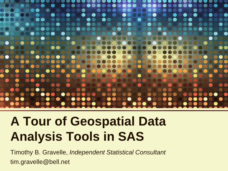
Reading in spatial data: Google Earth
(.kml) files
• Ex.: reading in the coordinates for the
proposed route of the Northern Gateway
pipeline (AB and BC):FILENAME ng "C:\NG\Northern Gateway path.kml";
DATA ng_0;
INFILE ng DSD dlm=', ' LRECL=32767 RECFM=n;
FORMAT LON LAT 20.16;
FORMAT LON LAT 20.16;
INPUT x $char1024. @;
strt=index(x,'<coordinates>')+14;
INPUT @strt @;
DO UNTIL(lon=.);
INPUT LON ?? LAT ?? ELEVATION ??;
IF LON ^= . THEN OUTPUT;
END;
KEEP LON LAT;
STOP;
RUN;11

12
Creating maps: PROC GMAP

Creating maps: PROC GMAP
• SAS makes it easy to create heat maps
(choropleth maps), plotting different levels of
a variable for different geographic areas.
• Ex.: a map of Boston showing the spatial
distribution of English language ability
(Statistics Without Borders project).
• A map was created by merging the census
tract TIGER/Line shapefile for Boston and
American Community Survey data:
13

Creating maps: PROC GMAP
FILENAME mapct "C:\SWB\tl_2010_25025_tract10.shp";
FILENAME langct "C:\SWB\ACS_10_5YR_B16001_with_ann.csv";
PROC MAPIMPORT DATAFILE=mapct OUT=map_0;
RUN;
DATA map_1 (DROP=COUNTY: STATE: NAME: INT: FUNC: MTFCC: );
SET map_0;
CT=INPUT(SUBSTR(GEOID10,6,6), 7.2); FORMAT CT 7.2;
IF (1601.01<=CT<=1606.99) OR (1701.00<=CT<=1708.99)
OR CT=9815.02 OR (1801.00<=CT<=1805.99) THEN DELETE;
/* DELETE CTs COMPRISING CHELSEA, REVERE & WINTHROP */
IF ALAND10>0;
/* DELETE CTs WITH NO LAND AREA */
RUN;
PROC SORT DATA=map_1;
BY CT;
RUN;
14

Creating maps: PROC GMAP
DATA lang_0;
INFILE langct FIRSTOBS=7 DSD DLM="," MISSOVER LRECL=32767;
LENGTH GEO_ID $ 20;
INPUT GEO_ID $ [...LOTS OF OTHER VARIABLES];
INFORMAT GEO_ID $20. VD1--mVD119 best12.;
FORMAT GEO_ID $20. VD1--mVD119 best12.;
DROP m: GEO_ID2 GEO_ID_DISPLAY;
CT=INPUT(SUBSTR(GEO_ID,15,6), 7.2); FORMAT CT 7.2;
IF (1601.01<=CT<=1606.99) OR (1701.00<=CT<=1708.99)
OR CT=9815.02 OR (1801.00<=CT<=1805.99) THEN DELETE;
/* DELETE CTs COMPRISING CHELSEA, REVERE & WINTHROP */
RUN;
DATA lang_1;
SET lang_0;
TOTAL_LTVW=SUM(VD5,VD8, [...] ,VD116,VD119);
/* GET THE TOTAL COUNT OF “LESS THAN VERY WELL”
ENGLISH SPEAKERS, ALL LANGUAGES */
RUN;
15

Creating maps: PROC GMAP
PROC SORT DATA=lang_1;
BY CT;
RUN;
FILENAME gout "C:\SWB\Boston Map 2012 08 14.png";
GOPTIONS RESET=ALL DEVICE=jpeg GSFNAME=gout YMAX=7.5in;
PROC GMAP MAP=map_1 DATA=lang_1;
ID CT;
CHORO TOTAL_LTVW /LEVELS=6 CDEFAULT=DARKGRAY;
LABEL TOTAL_LTVW=
"Count, Speak English ''Less than Very Well'')";
LEGEND1 ACROSS=3 DOWN=2;
RUN; QUIT;
16

17

Geocoding: PROC GEOCODE
• Refers to the appending of location (latitude-
longitude) information.
• SAS has well-developed built-in tools for US
data: ZIP, ZIP+4, address-based geocoding.
• Canadian and British geocoding was
introduced in SAS 9.4.
18
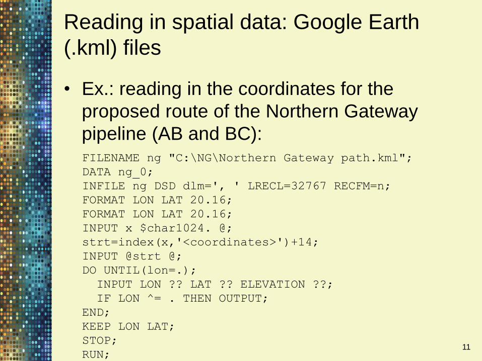
Geocoding: PROC GEOCODE
• Example – US survey data with ZIP codes in
dataset:
PROC GEOCODE DATA=data_1
METHOD=ZIP
OUT=data_2
LOOKUP=sashelp.zipcode
ADDRESSSTATEVAR=STATE
ADDRESSZIPVAR=ZIP
LOOKUPSTATEVAR=STATECODE
LOOKUPZIPVAR=ZIP
LOOKUPXVAR=X
LOOKUPYVAR=Y;
RUN;19

Geocoding: getting creative
• You may need to go beyond the built-in
capabilities of PROC GEOCODE – e.g.,
geocoding Canadian data using FSAs:
PROC MAPIMPORT DATAFILE=
"C:\Census11\gfsa000b11a_e.shp"
OUT=map_0;
RUN;
DATA map_1 (RENAME=(CFSAUID=FSA));
SET map_0;
RUN;
PROC SORT DATA=map_1;
BY FSA;
RUN;20

Geocoding: getting creative
%ANNOMAC;
%CENTROID(map_1, fsa_1, FSA, segonly=1);
DATA data_2;
LENGTH _MATCHED_ $ 50;
MERGE data_1 (IN=A) fsa_1;
BY FSA;
IF A=1;
IF X~=. AND Y~=. THEN _MATCHED_=
"Census 2011 FSA shapefile";
ELSE _MATCHED_="None";
RUN;
21

Dealing with map projections:
PROC GPROJECT
22
Source: Statistics Canada,
http://www12.statcan.gc.ca/census-recensement/
2011/ref/dict/figures/figure14-dict-eng.cfm

Dealing with map projections:
PROC GPROJECT
• One wrinkle is that SAS has no facility for
telling you if a shapefile is projected or not (or
which projection is being used).
• There functions in the sp and rgdal
packages in R to get this information.
• Ex.: “unprojecting” a map of the Kinder
Morgan Trans Mountain oil pipeline
expansion (originally in BC Albers projection):
PROC MAPIMPORT DATAFILE=
"C:\KM TM\KM_Pipeline_Expansion.shp"
OUT=tm_0b;
RUN;23

Dealing with map projections:
PROC GPROJECT
PROC GPROJECT DATA=tm_0b OUT=tm_1b
FROM="+proj=aea +lat_1=50 +lat_2=58.5
+lat_0=45 +lon_0=-126 +x_0=1000000 +y_0=0
+datum=WGS84 +units=m +no_defs +ellps=WGS84
+towgs84=0,0,0”
TO="+proj=longlat +datum=WGS84 +no_defs”;
ID SEGMENT;
RUN;
24

Dealing with map projections:
stepping out (momentarily) to R
library(sp)
library(rgdal)
setwd("C:/KM TM/")
map.1 <- readOGR(dsn = ".", "KM_Pipeline_Expansion")
map.1@proj4string
map.2 <- spTransform(map.1, CRS("+proj=longlat
+datum=WGS84"))
map.2@proj4string
25
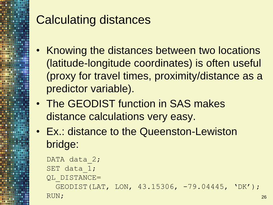
Calculating distances
• Knowing the distances between two locations
(latitude-longitude coordinates) is often useful
(proxy for travel times, proximity/distance as a
predictor variable).
• The GEODIST function in SAS makes
distance calculations very easy.
• Ex.: distance to the Queenston-Lewiston
bridge:
DATA data_2;
SET data_1;
QL_DISTANCE=
GEODIST(LAT, LON, 43.15306, -79.04445, ‘DK’);
RUN; 26

Calculating distances
• Calculating distances between large datasets
(e.g., a large survey dataset and a pipeline
route) is a little trickier.
• This can be done efficiently in PROC SQL
using a cross join (many-to-many join) and
then aggregating the data using record
(respondent) ID values.
27

Calculating distances
PROC SQL;
CREATE TABLE data_3a AS
SELECT D2.CASEID, D2.LAT, D2.LON,
GEODIST(D2.LAT, D2.LON, NG.LAT, NG.LON)
AS DISTANCE_PIPELINE,
LOG(GEODIST(D2.LAT, D2.LON, NG.LAT, NG.LON)+1)
AS LN_DISTANCE_PIPELINE
FROM data_2 AS D2
CROSS JOIN ng_1 AS NG
ORDER BY D2.CASEID, CALCULATED DISTANCE_PIPELINE
;
28

Calculating distances
CREATE TABLE data_3b AS
SELECT D3A.CASEID,
MEAN(D3A.LAT) AS LAT,
MEAN(D3A.LON) AS LON,
MIN(D3A.DISTANCE_PIPELINE)
AS DISTANCE_PIPELINE,
MIN(D3A.LN_DISTANCE_PIPELINE)
AS LN_DISTANCE_PIPELINE
FROM data_3a AS D3A
GROUP BY CASEID
ORDER BY CASEID
;
29

Calculating distances
CREATE TABLE data_3c AS
SELECT D2.*,
D3B.DISTANCE_PIPELINE,
D3B.LN_DISTANCE_PIPELINE
FROM data_2 AS D2
LEFT JOIN data_3b AS D3B
ON D2.CASEID=D3B.CASEID
ORDER BY D2.CASEID
;
QUIT;
30

Straight-line vs. road distances
• One might think that road distances/travel
time would be a better measure than straight-
line/“as the crow flies” distance (as calculated
using the GEODIST function).
• Empirical research comparing the two has
found them to be very strongly correlated
(r2 = 0.94) (Boscoe et al. 2012). They are
thus practically interchangeable.Source: Boscoe, Francis P., Kevin A. Henry and Michael S. Zdeb. 2012. “A Nationwide
Comparison of Driving Distance Versus Straight-Line Distance to Hospitals.” Professional
Geographer 64(2): 188–96.
31

Straight-line vs. road distances
• An alternative is to make repeated calls to a
map service (e.g., Google Maps) and extract
the travel distance/time from the result (see
Mike Zdeb’s TASS presentation, June 2012).
• This offers the prospect of greater accuracy
but becomes impractical very quickly with
thousands of records/respondents and
thousands of destination points.
• Seconds/minutes of run time for the PROC
SQL method vs. hours/days.
32

Wrap-up
• There are many ways to bring together
different sources of data with spatial data to
answer interesting questions.
• The world is awash in spatial data – much of
it free.
• You don’t need to be a trained GIS analyst to
get started (but it helps to be friends with
one).
• Nor do you need a full-fledged GIS platform –
base SAS and SAS/GRAPH have many
useful facilities.33

Wouldn’t it be nice...?
• If SAS could read in Google Earth .kml files,
either directly or via the XML Mapper?
• If PROC GMAP could handle multiple map
layers?
• If PROC MAPIMPORT or PROC GPROJECT
had the ability to output (to the output
window, log, or a SAS dataset) information on
map projection?
34