Embed Size (px)
Citation preview

Geostatistical Assessment of Sampling Designs for Portuguese
Bottom Trawl Surveys
Ernesto Jardim1 <[email protected]> and Paulo J. Ribeiro Jr2 <[email protected]>
27th April 2006
1Instituto Nacional de Investigação Agrária e das Pescas, Av. Brasilia, 1449-006, Lisboa, Portugal
Tel: +351 213 027 093
2Departamento de Estatística, Universidade Federal do Paraná, C.P. 19.081 CEP: 80.060-000, Curitiba, Paraná, Brasil
Abstract
New sampling designs for the Autumn Portuguese bottom trawl survey (ptBTS) were investigated to explore
alternative spatial configurations and possible increments on sample size. The currently used stratified random design
and five proposals of systematic based designs were assessed by a simulation study, adopting a geostatistical approach
based on likelihood methods of inference. The construction of the designs was based on “informal” method to reflect
the practical constraints of bottom trawl surveys. The proposed designs were a regular design with 28 locations (S28),
two regular designs with extra regular added locations with 44 (S44) and 47 (S47) locations, a design which overlaps
the regular and stratified random design currently used with 45 locations (S45) and an high density regular design with
108 locations (S108), used just as a benchmark. The designs were assessed by computing bias, relative bias, mean
square error and coverages of confidence intervals. Additionally a variance ratio statistic between each study designs
and a corresponding random design with the same sample size was computed to separate out the effects of different
sample sizes and spatial configurations. The best performance design was S45 with lower variance, higher coverage
for confidence intervals and lower variance ratio. This result can be explained by the fact that this design combines
good parameter estimation properties of the random designs with good prediction properties of regular designs. In
general coverages of confidence intervals where lower than the nominal 95% level reflecting an underestimation of
variance. Another interesting fact were the lower coverages of confidence intervals computed by sampling statistics
1

for the random designs, for increasing spatial correlation and sample size. This result illustrates that in the presence
of spatial correlation, sampling statistics will underestimate variances according to the combined effect of spatial
correlation and sampling density.
2

1 Introduction
Fisheries surveys are the most important sampling process to estimate fish abundance as they provide independent
information on the number and weight of fish that exist on a specific area and period. Moreover this information can
be disaggregated by several biological parameters like age, length, maturity status, etc. Like other sampling procedures
the quality of the data obtained depends in part on the sampling design used to estimate the variables of interest.
For the last 20 to 30 years, bottom trawl surveys (BTS) have been carried out in Western European waters using
design-based strategies (Anon. 2002, 2003). However, if one assumes that the number of fish in a specific location
is positively correlated with the number of fish in nearby locations, then a geostatistical model can be adopted for
estimation and prediction and a model-based approach can be considered to define and assess the sampling design. On
the other hand geostatistical principles are widely accepted and can be regarded as a natural choice for modelling fish
abundance (see e.g. Rivoirard et al. 2000; Anon. 2004).
Thompson (1992) contrasts design-based and model-based approaches considering that under the former one assumes
the values of the variable of interest are fixed and the selection probabilities for inference are introduced by the design,
whereas under the latter one consider the observed properties of interest as realisations of random variables and carries
out inference based on their joint probability distribution. Hansen et al. (1983) points the key difference between
the two strategies by stating that design-based inference does not need to assume a model for the population, the
random selection of the sample provides the necessary randomisation, while the model-based inference is made on
the basis of an assumed model for the population, and the randomisation supplied by nature is considered sufficient.
If the model is appropriate for the problem at hand there will be an efficiency gain in inference and prediction with
model-based approaches, however a model misspecification can produce inaccurate conclusions. In our context, with
experience accumulated over 20 years of bottom trawls surveys within the study area, there is a fairly good idea of the
characteristics of the population and the risk of assuming an unreasonable model should be small.
Portuguese bottom trawl surveys (ptBTS) have been carried out on the Portuguese continental waters since June 1979
on board the R/V Noruega, twice a year in Summer and Autumn. The main objectives of these surveys are: (i) to
estimate indices of abundance and biomass of the most important commercial species; (ii) to describe the spatial
distribution of the most important commercial species, (iii) to collect individual biological parameters as maturity,
sex-ratio, weight, food habits, etc. (SESITS 1999). The target species are hake (Merluccius merluccius), horse
mackerel (Trachurus trachurus), mackerel (Scomber scombrus), blue whiting (Micromessistius poutassou), megrims
(Lepidorhombus boscii and L. whiffiagonis), monkfish (Lophius budegassa and L. piscatorius) and Norway lobster
(Nephrops norvegicus). A Norwegian Campbell Trawl 1800/96 (NCT) with a codend of 20 mm mesh size, mean
vertical opening of 4.8 m and mean horizontal opening between wings of 15.6 m has been used (Anon. 2002).
3

Between 1979 and 1980, a stratified random sampling design with 15 strata was adopted. Those strata were designed
using depth and geographical areas. In 1981 the number of strata were revised to 36. In 1989 the sampling design was
reviewed and a new stratification was defined using 12 sectors along the Portuguese continental coast subdivided into
4 depth ranges: 20-100m, 101-200m, 201-500m and 501-750 m, with a total of 48 strata. Due to constraints in the
vessel time available the sample size was established in 97 locations, which were allocated equally splited to obtain
2 locations in each stratum. The locations’ coordinates were selected randomly constraint by the historical records of
clear tow positions and other information about the sea floor, avoiding places where the fishery engine was not able
to trawl. This sampling plan was kept fixed over the years. The tow duration until 2001 was 60 minutes and since
2002 was set in 30 minutes, based on an experiment that showed no significant differences in the mean abundance and
length distribution between the two tow duration.
The present work investigated proposals of new sampling designs for the Autumn Portuguese bottom trawl survey
(ptBTS). We aimed at explore new spatial configurations and possible increases on sample size, which could be
achieved by e.g. reducing the hauling time (from 1 hour to 1/2 hour). A simulation study was performed to compare the
stratified random design which is currently used against five proposals of systematic based designs, which we called
the study designs. A model based geostatistical approach (Diggle and Ribeiro 2006) was adopted using likelihood
based methods of inference and conditional simulations to estimate fish abundance on the study area.
Section 2 describes the framework for the simulation study starting with the model specifications followed by the
description of the sampling designs and the setup for the simulation study, conducted in five steps as described in
(Section 2.3). The results of the simulation study comparing the study designs are presented in Section 3 and the
findings are discussed in Section 4.
2 Methods
The survey area considered for this work corresponds to the Southwest of the Portuguese Continental EEZ (between
Setubal’s Canyon and S.Vicent Cape). Before any calculation the mercator projection was transformed into an or-
thonormal space by converting longitude by the cosine of the mean latitude (Rivoirard et al. 2000). At Portuguese
latitude (38-42o) 1olat ≈ 60nm. The area has ≈ 1250nm2 and the maximum distance between two locations was
≈ 81nm(1.35olat).
4
2.1 Geostatistical framework
Fish in a certain area interact with each other looking for food, reproductive conditions, etc. Therefore it is natural to
consider that the abundance of fish between spatial locations is positively correlated such that the correlation decays
with increasing separation distances. This conjecture justifies adopting the spatial model as defined in geostatistics (see
e.g. Cressie 1993, Part 1) to describe and obtain predictions of fish abundance over an area. This approach contrasts
with the sampling theory (see e.g. Cochran 1960) where the correlation between observations is not taken into account.
Additionally, within the geostatistical approach it is possible to estimate the abundance variance from systematic
designs and the parameters of the correlation function allows for the definition of different phenomena. Sampling
theory estimates would be obtained as the particular case, in the absence spatial correlation. Possible concerns includes
the extra complexity given by the model choice and eventual difficulties in estimating the model parameters.
The spatial model assumed here is a log-Gaussian geostatistical model. This is a particular case of the Box-Cox
Gaussian transformed class of models discussed in Christensen et al. (2001). The data consists of the pair of vectors
(x,y) with elements (xi,yi) : i = 1, ...,n, where xi denote the coordinates of a spatial location within a study region
A ⊂ R2 and yi is the measurement of the abundance at this location. Denoting by zi the logarithm of this measurement,
the Gaussian model for the vector of variables Z can be written as:
Z(x) = S(x)+ ε (1)
where S(x) is a stationary Gaussian process at locations x, with E[S(x)] = µ, Var[S(x)] = σ2 and an isotropic correlation
function ρ(h) = Corr[S(x),S(x′)], where h = ‖x− x′‖ is the Euclidean distance between the locations x and x′; and the
terms ε are assumed to be mutually independent and identically distributed Gau(0,τ2). For the correlation function
ρ(h) we adopted the exponential function with algebraic form ρ(h) = exp{−h/φ} where φ is the correlation range
parameter such that ρ(h) ' 0.05 when h = 3φ. Within the usual geostatistical jargon (Isaaks and Srivastava 1989)
τ2 +σ2 is the (total) sill, σ2 is the partial sill, τ2 is the nugget effect and 3φ is the practical range.
Hereafter we use the notation [·] for the distribution of the quantity indicated within the brackets. The adopted
model defines [log(Y )] ∼ MVGau(µ1,Σ), i.e [Y ] is multivariate log-Gaussian with covariance matrix Σ parametrised
by (σ2,φ,τ2). Parameter estimates can be obtained by maximising the log-likelihood for this model, given by:
l(µ,σ2,φ,τ2) = −n
∑i=1
log(yi)−0.5{n log(2π)+ log|Σ|+(zi −1)′Σ−1(zi −1)}. (2)
Likelihood based methods for geostatistical models are discussed in detail in Diggle and Ribeiro (2006). For spatial
prediction consider first the prediction target T (x0) = exp{S(x0)}, i.e. the value of the process in the original measure-
5
ment scale at a vector of spatial locations x0. Typically xo defines a grid over the study area. From the properties of
the model above the predictive distribution [T (x)|Y ] is log-Gaussian with mean µT and variance σ2T given by:
µT = exp{E[S(x0)]+0.5 Var[S(x0)]}
σ2T = exp{2 E[S(x0)]+Var[S(x0)]}(exp{Var[S(x0)]}−1)
with
E[S(x0)] = µ+Σ′0Σ−1(Z −1µ)
Cov[S(x0)] = Σ−Σ′0Σ−1Σ0
where Σ0 is a matrix of covariances between the the variables at prediction locations x0 and the data locations x
and Var[S(x0)] is given by the diagonal elements of Cov[S(x0)]. In practice, we replace the model parameters in the
expressions above are by their maximum likelihood estimates.
Under the model assumptions, [T |Y ] is multivariate log-Gaussian and it is therefore possible to make inferences not
only about prediction means and variances but also about other properties of interest. Although analytical expressions
can be obtained for some particular properties of interest, in general, we use conditional simulations to compute them.
Simulations from [T |Y ] are obtained by simulating from the multivariate Gaussian [S(x0)|Y ], and then exponentiating
the simulated values. Possible prediction targets can be denoted as functional F (S), for which inferences are obtained
by computing the quantity of interest on each of the conditional simulations. For instance, a functional of particular
interest in the present work was the global mean of the particular realisation of the stochastic process over the area,
which can be predicted by defining x0 as a grid over the area, obtaining the conditional simulations and computing the
mean value for each conditional simulation. More generally other quantities of possible interest as, for instance, the
percentage of the area for which the abundance is above a certain threshold, can be computed in a similar manner.
2.2 Sampling designs
In general, survey sampling design is about choosing the sample size n and the sample locations x from which data Y
can be used to predict any functional of the process. In the case of the ptBTS some particularities must be taken into
account: (i) the survey targets several species which may have different statistical and spatial behaviours; (ii) for each
species several variables are collected (weight, length, number, etc.); (iii) the sampling is destructive and replicates
can not be obtained; (iv) the variability of observed fish abundance is typically high, (v) the planned sampling design
6

may be unattained in practice due to unpredictable commercial fishing activity at the sampling area, bad sea conditions
and other possible operational constraints.
Optimal designs can be obtained formally, by defining a criteria and finding the set of sampling locations which min-
imises some sort of loss function, as e.g. discussed in Diggle and Lophaven 2006. On the other hand, designs can
be defined informally by arbitrarily defining locations which compromises between statistical principles and opera-
tional constraints. Both are valid for geostatiscal inference as described in Section 2.1 provided that the locations x
are fixed and stochastically independent of the observed variable Y . The above characteristics of the ptBTS makes it
very complex to set a suitable criteria to define a loss function to be minimized w.r.t. the designs. Additionally, costs
of a ship at sea are mainly day based and not haul based and increasing the sample sizes has to consider groups of
samples instead of the addition of individual points. Therefore, our approach was to construct the proposed designs
informally trying to accommodate: (i) historical information about hake and horse mackerel abundance distribution
(Anon. 2002; Jardim 2004), (ii) geostatistical principles about the estimation of correlation parameters (e.g. see Isaaks
and Srivastava 1989; Cressie 1993; Muller 2001) and (iii) operational constraints like known trawlable grounds and
minimum distance between hauls.
The study designs included the design currently adopted for this survey, named “ACTUAL” with 20 locations, and
five systematic based sampling designs. The systematic based designs were defined based on two possible increments
in the sample size: a ≈ 40% increment, which is expected to be achievable in practice by reducing haul time from 1
hour to 1/2 hour; and a ≈ 60% increment, which could be achieved in practice by adding to the previous increment an
allocation of higher sampling density to this area in order to cover the highest density of hake recruits historically found
within this zone. These designs are denoted by “S” followed by a number corresponding to the sample size. For the
former increment a regular design named “S28” was proposed and three designs were proposed for the latter: “S45”
overlaps the designs ACTUAL and S28, allowing direct comparison with the previous designs; “S44” and “S47” are
two infill designs (Diggle and Lophaven 2006) obtained by augmenting S28 with a set of locations positioned regularly
at smaller distances, aiming to better estimate the correlation parameter and, in particular, the noise-to-signal ratio.
S44 was built by defining a single denser sampling zone and S47 by adding three areas with denser sampling. A sixth
design “S108” was defined to be used as reference with twice the density of S28. A feature of these choices is the
possible confounding between the effect of sample sizes and spatial configuration. We circunvect this problem by
building six additional designs with the same sample size as the study designs and with locations randomly chosen
within the study area. We denote these by “R” followed by the number of corresponding locations. Each random
design contains all the locations of the previous one such that the results are comparable without effects of the random
allocation of the sampling locations. The study and corresponding random designs are shown in Figure 1.
7

2.3 Simulation study
The simulation study was carried out in five steps as follows.
Step 1 Define a set of study designs. The sampling designs described in Section 2.2 are denoted by Λd : d =
1, . . . ,12, with d = 1, . . . ,6 for the study designs and d = 7, . . . ,12 for the corresponding random designs,
respectively.
Step 2 Define a set of correlation parameters. Based on the analysis of historical data of hake and horse
mackerel spatial distribution and defining τ2REL = τ2/(τ2 + σ2), a set of model parameters θp : p =
1, ...,P was defined by all combinations of φ = {0.05,0.1,0.15,0.2,0.25,0.3,0.35,0.4}olat and τ2REL =
{0,0.1,0.2,0.3,0.4,0.5}. The values of σ2 are given by setting σ2 + τ2 = 1.
Step 3 Simulate data. For each parameter set θp we obtained S=200 simulations Yps : s = 1, . . . ,S from [Y ] on a
regular grid of 8781 locations under the model described in Section 2.1. Each simulation Yps approximates
a possible realisation of the process within the study area from which we computed the mean value µps.
For each Yps we extracted the data Ypds at the locations of the sampling designs Λd .
Step 4 Estimate correlation parameters. For each Ypds obtain maximum likelihood estimates (MLE’s) θpds of
the model parameter.
Step 5 Simulating from the predictive distribution. A prediction grid x0 with 1105 locations and the estimates
θpsd were used to obtain C=150 simulations Ypdsc : c = 1, . . . ,C of the conditional distribution [T (x0)|Y ]
which were averaged to produce ¯Ypdsc.
2.4 Analysis of simulation results
The simulation study requires maximum likelihood estimates for the model parameters which are obtained numeri-
cally. Therefore a set of summary statistics was computed in order to check the consistency of the results. We have
recorded rates of non-convergence of the minimization algorithm; estimates which coincides with the limiting values
imposed to the minimization algorithm (φ = 3 and τ2REL = 0.91); absence of spatial correlation (φ = 0) and values of
the parameter estimates which are considered atypical for the problem at hand (φ > 0.7 and τ2REL > 0.67).
The 48 parameters set (θp), 12 sampling designs (∆d), 200 data simulations (Ypsd) and 150 conditional simulations
(Ypsdc) produced 17.28 million estimates of abundance which were used to compare the designs. For each design
we have computed the estimator µpsd = C−1 ∑c¯Ypdsc of mean abundance µps which has variance Var(µpsd) = ¯ρAA +
∑ni ∑n
j wiw j ρi j − 2∑ni wi ¯ρiA, where ¯ρAA is the mean covariance within the area, estimated by the average covariance
8

between the prediction grid locations (x0); w are kriging weights; ρi j is the covariance between a pair of data locations;
and ¯ρiA is the average covariance between each data locations and the area discretized by the prediction grid x0 (Isaaks
and Srivastava 1989).
We used bias, relative bias, mean square error (MSE), confidence intervals coverage and ratio of variances to assess
the simulation results, comparing the estimates of the abundance provided by the study designs. For each design these
statistics were averaged over all the simulations (s) and parameter sets (p) or groups of parameters sets. Considering
the difference between the abundance estimates µpsd and simulated means µps, bias was computed by the difference,
relative bias was computed by the difference over the estimate µps and MSE was computed by the square of the
difference. For each estimate µpds a 95\% confidence interval for µps, given by CI(µpsd) = µpsd ± 1.96√
Var(µpsd),
was constructed and the coverage of the confidence intervals δ were computed by the proportion of the intervals which
contained the value of µps over all the simulations. This statistic was introduced to help assessing the quality of the
variance estimates. At least, we called ratio of variances a statistic ξ obtained by dividing the variance Var(µ psd)
of each study design by the random design with the same size. Notice that the single difference among each pair of
designs with the same size was the spatial configuration of the locations and ξ isolated this effect. Finally we used the
results from the six random designs to contrast sampling design based and geostatistical based estimates.
All the analysis were performed with the R software (R Development Core Team 2005) and the add-on packages geoR
(Ribeiro Jr. and Diggle 2001) and RandomFields (Schlather 2001).
3 Results
Table 1 summarises the analysis of historical data showing parameter estimates for a sequence of years. This aims to
gather information on reasonable values for the model parameters. Notice that units for φ are given in degrees and, for
the adopted exponential correlation model, the practical range is given by 3φ and also included in the Table (r) with
units in nautical miles. The values of τ2REL = 1 estimated in some years indicates an uncorrelated spatial process and
for such cases estimates of φ equals to zero. For most of the cases τ2REL was estimated as zero due to the lack of nearby
locations in the sampling plan and the behaviour of the exponential correlation function at short distances. Given that
there is no information in the data about the spatial correlation at distances smaller than the smallest separation distance
between a pair of location, this parameter can not be estimated properly and the results depend on the behaviour of the
correlation function near the origin.
Table 2 summarizes the checks of the results of the parameter estimates which were considered satisfactory and
coherent. The highest rate of lack of convergence was 0.6% for the designs ACTUAL and R20. Estimates of φ equals
to the upper limit imposed to the algorithm were, in the worst case, 0.9% for R28 and R47 and for τ2REL it was 1.2% for
9

R28 . In general there was a slight worst performance of the random designs but this is irrelevant for the objectives of
this study. Those simulations were not considered for subsequent analysis. Lack or weak spatial correlation given by
φ = 0 and/or τ2REL > 0.67 was found in about 35% of the simulations for the designs with fewer number of locations,
and this rate decreases as the sample size increases, down to below 10% for the largest designs. For both statistics
the study designs showed slightly higher values than the corresponding random designs. Identification of weakly
correlated spatial processes in part of the simulations was indeed expected to occur given the low values of φ (0.05
and 0.1) used in the simulations. The number of cases that presented atypical estimates for φ were slightly higher for
random designs, with a maximum of 2.6% for R44 and R45, but were considered to be within an acceptable range
given the high variability of the estimator.
Figure 2 shows square bias, variance and MSE obtained from the estimates of correlation parameters φ and τ2REL. For
τ2REL the majority of the designs presented similar patterns with a small contribution of bias to the MSE and increasing
values of MSE for higher true parameter values. The designs ACTUAL, S28 and R20 behaved differently with higher
values of bias at low values of τ2REL that pushed MSE to higher values. As an effect of the sample sizes, the absolute
values of MSE defines 3 groups composed by designs with 20 and 28 locations, designs with 44, 45 and 47 locations,
and designs with 108 locations; with decreasing values of MSE among them, respectively. MSE increases with the
increase of the true value of φ and its absolute value decreases slightly with the increasing sample sizes. All designs
presented a similar pattern with the variance contributing more than bias to the MSE. The study designs showed a
slightly higher relative contribution of the variance to MSE compared with the random designs.
Table 3 shows geostatistical abundance estimates (µ) and their bias, relative bias, variance, MSE and 95% confidence
interval coverage for both sets of designs. Additionally the table also shows statistics based on sampling theory
obtained for random designs. For subsequent analysis the designs S108 and R108 were regarded just as benchmarks
since they are unrealistic for practical implementation. Bias were quite small in all situations and can be considered
negligible with higher relative bias of 0.014 for S28. All random designs showed a negative bias whereas all study
designs showed a positive one. Variances estimated by study designs were lower than the ones for the corresponding
random designs. For random designs the variance decays with increasing sample sizes, whereas study designs behaved
differently with S45 presenting the lowest variance with greater differences between S44, S45 and S47 and R44, R45
and R47. The same is valid for MSE, since the bias were small, however with higher absolute values supporting
our claim that bias were not relevant for the purpose of this work. The coverages of confidence intervals (δ) were
lower than the nominal level of 95% excepted for S108 and R108, reflecting an underestimation of the variance.
Considering the designs individually it can be seen that ACTUAL, S28 and S45 showed a lower underestimation
than the equivalent random designs. To better investigate this Figure 3 presents values of δ splitted by three levels
of correlation (low={0.05, 0.1}, med={0.15, 0.20, 0.25}, high={0.3, 0.35, 0.4}). For geostatistical estimates the
10
coverages δ increases with higher true values of φ and larger sample sizes, whereas sampling statistics showed a
different pattern, with maximum values for R44 for low and medium correlation levels and for R28 for high correlation
levels. This behaviour is more noticeable for stronger spatial correlation, in particular, the largest designs showed lower
confidence interval coverage pointing for a more pronounced underestimation of the variance.
Logarithms of the variance ratios between corresponding “S” and “R” designs are presented in Table 3. Without
considering S108 for the reasons stated before, the best result was found for S45 (−0.208) and the worst for S28
(−0.108). This must be balanced by the fact that S45 showed a lower variance underestimation than R45, with the
opposite happening for S44/R44 and S47/R47, so, in reality, value of ξ is smaller for S45 than for S44 and S47.
4 Discussion
The choice of sampling designs for BTS is subject to several practical constraints and this has motivated the adoption
of informally defined designs which accommodated several sources of information like fishing grounds, haul duration,
previous knowledge of the spatial distribution of hake and horse mackerel, among others, which could not be incorpo-
rated into a design criteria in an objective way. The fact that this can generate designs with different sample sizes is a
drawback of this approach. However, implementing a systematic design on an irregular spatial domain is also likely to
provide designs with different sample sizes, depending on the starting location. Costs of hauling are relatively small
when compared with the fixed costs associated with a vessel’s working day and increasing sample sizes for a BTS
must consider sets of locations which can be sampled in one working day. For these reasons the different sample sizes
of each design are not just a feature of the adopted approach but also a result of the BTS particularities.
The confounding effects of sample size and spatial configuration of the proposed designs jeopardized the comparison
of their ability in estimating the abundance. To circunvect this limitation a methodology to compare designs with
different sample sizes and spatial configurations was required. To deal with this issue we’ve introduced a mean
abundance variance ratio statistic, between the study designs and a corresponding simulated random design with the
same sample size.
In fisheries science the main objective for the spatial analysis usually lies in predicting the distribution of the marine
resource, aiming, for instance, to define marine protected areas and to compute abundance indices for stock assessment
models (Anon. (2004)). For such situations the model parameters are not the focus of the study, but just a device to
better predict the abundance. Muller (2001) points that the optimality of spatial sampling designs depends on the
objectives, showing that ideal designs to estimate covariance parameters of the stochastic process are not the same
to predict the value of the stochastic process in a specific location and/or to estimate global abundance. We have not
11

compared the study designs with respect to the estimation of the covariance parameters provided that our main concern
was spatial prediction of abundance.
The choice of the parameter estimation method was a relevant issue in the context of this work. The absence of
a formal criteria to identify the “best” design naturally led to the use of geostatistical simulations to compare the
proposed designs. To carry out a simulation study it is useful to have an objective method capable of producing single
estimates of the model parameters. Within traditional geostatistical methods (e.g. Isaaks and Srivastava 1989; Cressie
1993; Rivoirard et al. 2000, Goovaerts (1997)), the estimation entangles subjective analyst’s intervention to define
some empirical variogram parameters such as lag interval, lag tolerance and estimator for the empirical variogram.
Likelihood based inference produces estimates of the covariance parameters without a subjective intervention of the
data analyst, allowing for automatization of the estimation process, which is suitable for simulation studies. For
the current work we have also used other methods such restricted maximum likelihood (REML) and weighted least
squares, but they have produced worse rates of convergence in the simulation study. In particular the REML presented
an high instability with a high frequency of atypical results for φ. An aspect of parameter estimation for geostatistical
models which is highlighted when using likelihood based methods is regarded to parameter identification due to
over-parametrized or poorly identifiable models (see e.g. Zhang (2004)). To avoid over parametrization we used a
log-transformation and the process was considered isotropic, avoiding the inclusion of three parameters on the model:
the box-cox transformation parameter (Box and Cox 1964) and the two anisotropy parameters, angle and ratio. The
choice of the log transformation was supported by the analysis of historical data and does not impact the comparison
of the designs, given that the relative performance of each design will not be affected by the transformation. A point
of concern with the log transformation was the existence of zero values which, in the analysis of the historical data,
were treated as measurement error and included in the analysis with a translation of the observed values, by adding a
small amount to all observations. However, it must be noted this is not always recommended and, in particular, if the
stock is concentrated on small schools that cause discontinuities on the spatial distribution, these transformations will
not produce satisfactory results. Concerning anisotropy, a complete simulation procedure was carried out considering
a fixed anisotropy angle on the north-south direction and an anisotropy ratio of 1, 1.5 or 2. As expected, the absolute
values obtained were different but the overall relative performance the designs was the same, supporting our decision
to report results only for the isotropic model.
Overall, maximum likelihood estimation of the model parameters was considered satisfactory and checks of the con-
sistence of simulation analysis did not reveal major problems with the parameters estimates showing the designs
performed equally well and with similar patterns on bias and MSE.
A major motivation for performing a simulation study was the possibility to use a wide range of covariance parameters,
reflecting different possible spatial behaviours which implicitly evaluates robustness. Furthermore, the results can be
12

retained for all species with a spatial behaviour covered by these parameters.
From a space-time modeling perspective, one of the most interesting analysis for fisheries science is the fluctuation of
the stochastic process over time contrasted with the specific realization in a particular time. Therefore the comparison
with the mean of the realisations (µps) was considered more relevant then to the mean of the underlying process (µ) for
the computation of bias and variability. The results showed higher bias for study designs when compared with random
designs, but in both cases showing low values which were considered negligible for the purposes of this work. This
conclusion was also supported by the fact that MSE showed a similar relative behaviour as variance.
Apart from the design S108, which was introduced as a benchmark and not suitable for implementation, the design
that performed better was S45 with lower variance, confidence interval coverage closer to the nominal level of 95%
and lower variance ratio (Table 3). One possible reason is the balance between good estimation properties given by the
random locations and good predictive properties given by the systematic locations, however the complexity of the BTS
objectives makes it impossible to find a full explanation for this results. A possible indicator of the predictive properties
is the average distance between the designs and the prediction grid locations, which reflects the extrapolation needed
to predict over a grid. We found that S45 had an average of 2.61nm whereas for S47 the value is 2.72nm, explaining
in part the S45 performance.
These results are in agreement with Diggle and Lophaven (2006) who showed that lattice plus closed pairs designs
(similar to S45) performed better than lattice plus in-fill designs (similar to S44 and S47) for accurate prediction of the
underlying spatial phenomenon. The combination of random and systematic designs like S45 is seldom considered in
practice and we are not aware of recommendations of such designs for BTS.
It was interesting to notice that most designs presented a coverage of confidence intervals below the nominal level of
95% revealing the variances were underestimated. It was not fully clear how to use such results to correct variance
estimation and further investigation is needed on the subject. Care must be taken when looking at variance ratios since
underestimated denominators will produce higher ratios which can mask the results. This was the case of S45 when
comparing to S47 and S44, supporting our conclusions about S45.
Another result of our work was the assessment of abundance estimates from random designs by sampling statistics,
the most common procedure for fisheries surveys (Anon. 2004), under the presence of spatial correlation. In such
conditions an increase in sample size may not provide a proportional increase in the quantity of information due to
the partial redundancy of information under spatial correlation. Results obtained for coverages of confidence intervals
illustrated this (Table 3 and Figure 3), with smaller coverages for larger sample sizes and higher spatial correlation,
reflecting an over estimation of the degrees of freedom. The overestimation of the degrees of freedom led to an under-
estimation of prediction standart errors producing the smaller coverages. These fundings support claims to consider
geostatistical methods to estimate fish abundance, such that correlation between locations is explicitly considered in
13

the analysis, and highlighting the importance of verifying the assumptions behing sampling theory before computing
the uncertainty of abundance estimates.
5 Acknowledgements
The authors would like to thank the scientific teams evolved in the Portuguese Bottom Trawl Surveys, in particular
the coordinator Fátima Cardador, and the comments by Manuela Azevedo. This work was carried out within the
IPIMAR’s project NeoMAv (QCA-3/MARE-FEDER, http://ipimar-iniap.ipimar.pt/neomav) and was co-financed by
project POCTI/MATH/44082/2002.
References
Anon. 2002. Report of the International Bottom Trawl Survey Working Group. International Council for the Exploita-
tion of the Sea (ICES), ICES CM 2002/D:03.
Anon. 2003. Report of the International Bottom Trawl Survey Working Group. International Council for the Exploita-
tion of the Sea (ICES), ICES CM 2003/D:05.
Anon. 2004. Report of the Workshop on Survey Design and Data Analysis. International Council for the Exploitation
of the Sea (ICES), ICES CM 2004/B:07.
Box, G., and Cox, D. 1964. An Analysis of Transformations. Journal of the Royal Statistical Society Series B 26:
211–243.
Christensen, O., Diggle, P., and Ribeiro Jr, P. 2001. Analysing positive-valued spatial data: the transformed gaussian
model. In GeoENV III - Geostatistics for Environmental Applications Edited by P. Monestiez, D. Allard, and
Froidevaux, Quantitative Geology and Geostatistics, vol. 11. Kluwer, pp. 287–298.
Cochran, W. 1960. Sampling Techniques. Statistics. John Wiley & Sons, INC, New York.
Cressie, N. 1993. Statistics for spatial data - Revised Edition. John Wiley and Sons, New York.
Diggle, P., and Ribeiro, P. 2006. Model-based Geostatistics. Springer, New York. In press.
Diggle, P. J., and Lophaven, S. 2006. Bayesian geostatistical design. Scandinavian Journal of Statistics 33: 55–64.
Goovaerts, P. 1997. Geostatistics for Natural Resources Evaluation. Oxford University Press, New York.
14

Hansen, M., Madow, W., and Tepping, B. 1983. An Evaluation of Model-Dependent and Probability-Sampling Infer-
ences in Sample Surveys. Journal of the American Statistical Association 78: 776–793.
Isaaks, E., and Srivastava, M. 1989. An Introduction to Applied Geostatistics. Oxford University Press, New York.
Jardim, E. 2004. Visualizing hake recruitment - a non-stationary process. In geoENV IV - Geostatistics for Environ-
mental Applications Edited by X. Sanchez-Vila, J. Carrera, and J. J. Gómez-Hernandéz, Quantitative Geology and
Geostatistics, vol. 13. Kluwer Academic Publishers, London, pp. 508–509.
Muller, W. 2001. Collecting Spatial Data - Optimum Design of Experiments for Random Fields. Contributions to
statistics, 2nd edn. Physica-Verlag, Heidelberg.
R Development Core Team 2005. R: A language and environment for statistical computing. R Foundation for Statis-
tical Computing, Vienna, Austria. ISBN 3-900051-07-0.
Ribeiro Jr., P., and Diggle, P. 2001. geoR: a package from geostatistical analysis. R-NEWS 1: 15–18.
Rivoirard, J., Simmonds, J., Foote, K., Fernandes, P., and Bez, N. 2000. Geostatistics for Estimating Fish Abundance.
Blackwell Science, London, England.
Schlather, M. 2001. Simulation and analysis of random fields. R News 1: 18–20.
Thompson, S. 1992. Sampling. Statistics. John Wiley & Sons, INC, New York.
Zhang, H. 2004. Inconsistent estimation and asymptotically equal interpolations in model-based geostatistics. Journal
of the American Statistical Association 99: 250 – 261.
15

Table 1: Exponential covariance function parameters (φ,τ2REL) and the geostatistical range (r) estimated yearly (1990-
2004) for hake and horse mackerel abundance. The values of φ are presented in degrees of latitude and range innautical miles. The maximum distance between pairs of locations was 63nm.
Hake Horse mackerelφ(olat) r(nm) τ2
REL φ(olat) r(nm) τ2REL
1990 0.05 9.1 0.01 0.42 76.4 0.001991 0.14 24.4 0.63 0.49 88.9 0.431992 0.00 0.0 1.00 0.22 39.3 0.051993 0.05 9.3 0.00 0.00 0.0 1.001995 0.05 8.8 0.00 0.08 14.4 0.001997 0.14 24.8 0.00 0.21 38.6 0.421998 0.02 3.4 0.00 0.09 16.5 0.001999 0.10 17.8 0.00 0.09 16.0 0.002000 0.03 4.6 0.00 0.16 29.5 0.002001 0.07 12.9 0.00 0.42 75.7 0.062002 0.00 0.0 1.00 0.05 8.9 0.002003 0.33 59.0 0.00 0.34 62.0 0.002004 0.09 15.4 0.00 0.09 17.0 0.00
Table 2: Statistics to provide simulation quality assessment (in percentages) for both design sets and all sample sizes:non-convergence of the minimization algorithm (non-conv); cases truncated by the limits imposed to the minimizationalgorithm (φ = 3 and τ2
REL = 0.91); uncorrelated cases (φ = 0); and atypical values of the correlation parameters(φ > 0.7 and τ2
REL > 0.67).
statistic design sample size20 28 44 45 47 108
non-conv study 0.6 0.5 0.2 0.2 0.2 0.1random 0.6 0.4 0.2 0.2 0.2 0.1
φ = 3 study 0.7 0.5 0.7 0.7 0.5 0.2random 0.6 0.9 0.8 0.8 0.9 0.1
τ2REL = 0.91 study 0.7 0.7 1.0 0.9 0.8 0.4
random 0.8 1.2 1.1 1.1 1.1 0.2φ = 0 study 36.3 33.0 20.7 20.6 18.0 5.3
random 32.8 28.5 18.1 17.2 16.2 3.3φ > 0.7 study 1.3 1.6 1.9 1.9 1.8 1.4
random 1.8 2.2 2.6 2.6 2.4 1.7τ2
REL > 0.67 study 38.5 35.8 24.2 24.7 21.8 10.0random 35.0 31.6 22.1 21.1 20.3 7.6
16

Table 3: Summary statistics per sets of sampling designs and sample size. Geostatistical abundance estimates (µ), bias(bias(µ)), relative bias (biasr(µ)), variance (var(µ)), mean square error (MSE) and 95% confidence interval coverage(δ(µ)). Mean log variance ratios per sampling design type (ξ) measures the relative log effect of the systematic baseddesigns configuration with relation to the random designs. The last six rows present the same statistics estimated forrandom designs by sampling statistics.
method statistic design number of locations20 28 44 45 47 108
geostatistics µ study 1.658 1.662 1.649 1.657 1.651 1.641random 1.631 1.624 1.625 1.624 1.625 1.625
bias(µ) study 0.025 0.030 0.016 0.026 0.019 0.008random -0.001 -0.008 -0.007 -0.009 -0.008 -0.007
biasr(µ) study 0.012 0.014 0.003 0.012 0.005 0.001random -0.004 -0.008 -0.005 -0.006 -0.005 -0.005
var(µ) study 0.136 0.108 0.092 0.086 0.089 0.081random 0.168 0.129 0.113 0.112 0.112 0.097
MSE(µ) study 0.272 0.196 0.164 0.144 0.154 0.104random 0.321 0.230 0.173 0.171 0.171 0.124
δ(µ) study 0.908 0.922 0.907 0.939 0.920 0.960random 0.895 0.909 0.937 0.934 0.934 0.954
ξ stu/rnd -0.128 -0.107 -0.150 -0.208 -0.179 -0.228sampling statistics Y random 1.615 1.619 1.618 1.616 1.618 1.622
bias(Y ) random -0.017 -0.014 -0.014 -0.017 -0.015 -0.010biasr(Y ) random -0.017 -0.014 -0.013 -0.014 -0.014 -0.006var(Y ) random 0.197 0.146 0.091 0.088 0.085 0.037
MSE(µ) random 4.133 4.238 4.109 4.083 4.090 4.073δ(Y ) random 0.900 0.910 0.908 0.900 0.896 0.840
17

Figure 1: Sampling designs and the study area (southwest of Portugal). Each plot shows the sample locations, thebathimetric isoline of 500m and 20m and the coast line. The sampling design name is presented on the top left cornerof the plots. The top row shows the study designs and the bottom row the random designs.
lon
lat
Sines500m
20m
ACTUAL(n=20)
37.0
37.4
37.8
38.2
lon
lat
Sines500m
20m
S28
−7.3 −7.1 −6.9
lon
lat
Sines500m
20m
S44
lon
lat
Sines500m
20m
S45
−7.3 −7.1 −6.9
lon
lat
Sines500m
20m
S47
lon
lat
Sines500m
20m
S108
−7.3 −7.1 −6.9
lon
lat
Sines500m
20m
R20
−7.3 −7.1 −6.9
lon
lat
Sines500m
20m
R28
lon
lat
Sines500m
20m
R44
−7.3 −7.1 −6.9
lon
lat
Sines500m
20m
R45
lon
lat
Sines500m
20m
R47
−7.3 −7.1 −6.9
lon
lat
Sines500m
20m
R108
37.0
37.4
37.8
38.2
18
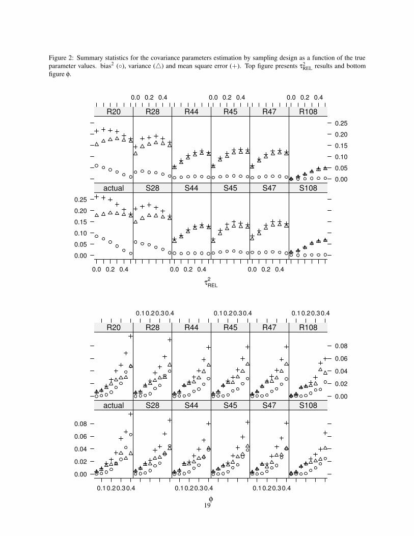
Figure 2: Summary statistics for the covariance parameters estimation by sampling design as a function of the trueparameter values. bias2 (◦), variance (4) and mean square error (+). Top figure presents τ2
REL results and bottomfigure φ.
τREL2
0.00
0.05
0.10
0.15
0.20
0.25
0.0 0.2 0.4
actual S28
0.0 0.2 0.4
S44 S45
0.0 0.2 0.4
S47 S108
R20
0.0 0.2 0.4
R28 R44
0.0 0.2 0.4
R45 R47
0.0 0.2 0.4
0.00
0.05
0.10
0.15
0.20
0.25
R108
φ
0.00
0.02
0.04
0.06
0.08
0.10.20.30.4
actual S28
0.10.20.30.4
S44 S45
0.10.20.30.4
S47 S108
R20
0.10.20.30.4
R28 R44
0.10.20.30.4
R45 R47
0.10.20.30.4
0.00
0.02
0.04
0.06
0.08
R108
19

Figure 3: Coverage of the confidence intervals (δ) for different φ levels (low = {0.05,0.1}, med{0.15,0.20,0.25}high = {0.30,0.35,0.40}) for estimates of abundance by sampling statistics for the random designs (+) and by geo-statistics for the study (o) and random designs (∗).
sample size
δ(µ~ )
0.80
0.85
0.90
0.95
20 28 44 45 47 108
** * * * *o o
o
oo
o
++
+ + ++
low0.80
0.85
0.90
0.95
* ** * *
*o
oo
o oo
+ + + + +
+
med0.80
0.85
0.90
0.95
* ** * *
*o
o oo
o
o
+ ++ + +
+
high
20