www.elsevier.com/locate/agrformet

Agricultural and Forest Meteorology 146 (2007) 173–188

Geostatistical modelling of air temperature in a mountainous

region of Northern Spain

Raquel Benavides a,*, Fernando Montes b, Agustın Rubio b, Koldo Osoro a

a SERIDA, Area de Sistemas de Produccion Animal, 33300 Villaviciosa, Asturias, Spainb Departamento de Silvopascicultura, Universidad Politecnica de Madrid, 28040 Madrid, Spain

Received 17 October 2006; received in revised form 23 May 2007; accepted 25 May 2007

Abstract

Air temperature is one of the most important factors affecting vegetation and controlling key ecological processes. Air

temperature models were compared in a mountainous region (Asturias in the North of Spain) derived from five geostatistical and

two regression models, using data for January (coolest month) and August (warmest month). The geostatistical models include the

ordinary kriging (OK), developed in the XY plane and in the X, Yand Z-axis (OKxyz), with zonal anisotropy in the Z-axis (variogram

fitting procedure developed in this study), and three techniques that introduce elevation as an explanatory variable: ordinary kriging

with external drift (OKED) and universal kriging, using the ordinary least squares (OLS) residuals to estimate the variogram (UK1)

or the generalised least squares (GLS) residuals (UK2). The OKED, UK1 and UK2 techniques were more satisfactory than OK in

terms of standard prediction error and mean absolute error, which were inferior by 1 8C, but OKxyz improved the results obtained

with those techniques. Moreover, OKxyz, OKED, UK1 and UK2 improved slightly the results of a regression model with UTM

coordinates and elevation data as independent variables in terms of bias (R1); whereas a complex regression model, which includes

altitude, latitude, distance to the sea and solar radiance as independent variables (R2), showed better results in terms of mean

absolute error, under 0.16 8C for both months. A second validation carried out with stations discarded for the interpolation showed a

greater similarity between the efficiency of R2 and the geostatistical techniques.

# 2007 Elsevier B.V. All rights reserved.

Keywords: Climate; Kriging; Mapping; Regression analysis; DEM

1. Introduction

Air temperature is one of the input variables for land

evaluation and characterisation systems, as well as

hydrological and ecological models. These models use

air temperature to drive processes such as evapotran-

spiration, soil decomposition, and plant productivity

(Dodson and Marks, 1997). Hence, forest management

and research need this climatic variable as a basis for

understanding many processes, as it is the main factor

* Corresponding author.

E-mail address: rbenavides@serida.org (R. Benavides).

0168-1923/$ – see front matter # 2007 Elsevier B.V. All rights reserved.

doi:10.1016/j.agrformet.2007.05.014

affecting vegetation distribution, in the sense that its

action is felt over wide areas of the earth’s surface (De

Phillips, 1951).

Air temperature is an important site characteristic

used in determining site suitability for agricultural and

forest crops (Hudson and Wackernagel, 1994), and it is

used in parameterizing the habitat of plant species

(Rubio et al., 2002; Sanchez-Palomares et al., 2003) and

in determining the patterns of vegetational zonation

(Richardson et al., 2004). Moreover, air temperature is a

factor related to plant productivity, as it is connected

with the length of the vegetative period and evapo-

transpiration. Different indexes have been developed for

relationships between components of climate and

R. Benavides et al. / Agricultural and Forest Meteorology 146 (2007) 173–188174

quantitative variables of vegetation communities. These

indexes are known as potential productivity indexes,

and they are reviewed in Serrada (1976), Hagglund

(1981) and Del Valle (2004). Finally, temperature can

be also considered as a limitation factor, and many

studies have been carried out with temperature as a

threshold for different processes, e.g. the minimum

temperature which may lead to lethal damage of tissue

or whole tree seedlings under different situations of

stand density, topography or soil preparation (Blennow,

1993, 1998).

Therefore, spatial modelling of climate variables,

such as air temperature, is of interest for forestry

science. However, these variables are not easy to obtain

because they appear as measurements at discrete points.

Consequently, many different methods have been

developed to generate regional maps from point data,

based on the continuity of temperature and its strong

dependency on elevation; on a global average,

temperature decreases around 0.65 8C/100 m in altitude

(Barry and Chorley, 1987; Gandullo, 1994; Lutgens and

Tarbuck, 1995), although this rate may vary with the

season and the geographic situation (Goodale et al.,

1998), and in relation to diurnal effects (Richardson

et al., 2004).

Different interpolation methods have been used to

model the spatial distribution of air temperature; the

most widely used being the inverse distance interpola-

tion weighting, Voronoi tessellation, regression analysis

or, more recently, geostatistical methods. Kurtzman and

Kadmon (1999) compared different methods (splines,

inverse distance weighting and multiple regression

analysis) for daily mean minimum and maximum

temperatures in Israel; Sanchez-Palomares et al. (1999)

developed maps of climate variables with polynomial

regressions based on the X and Y coordinates and

elevation in Spain. Relationships have been derived

between temperature and other topographic variables,

together with elevations, such as exposure, continen-

tality, latitude, and solar radiation. For example,

Goodale et al. (1998) and Ninyerola et al. (2000,

2005) used regression analysis and GIS techniques to

model different climate components in Ireland and

Spain, respectively. Marquınez et al. (2003) related

rainfalls in Asturias (Spain) with variables such as

distance to the sea and to the West (due to the

dominance of fronts from NW). Geostatistical techni-

ques have also been used: Lapen and Hayhoe (2003)

compared inverse distance weighting to geostatistical

methods (ordinary kriging (OK) and cokriging, and

ordinary kriging with external drift (OKED)) to

spatially model the seasonal and annual temperature

and total precipitation normals in the Great Lakes

(Ontario, Canada); Hudson and Wackernagel (1994)

mapped air temperature of Scotland using ordinary

kriging with external drift; and Ishida and Kawashima

(1993) used different kriging estimators, specially

cokriging estimators, to evaluate the usefulness of

these approaches in temperature modelling in Japan.

Approaches that include altitude (or depth) as a spatial

dimension (as ordinary kriging with Z anisotropy) have

been successfully applied for natural resources estima-

tion (Ayalew et al., 2002; Montes et al., 2005), but these

approaches have never been used for predicting climatic

variables.

Air temperature modelling in mountainous regions is

difficult and challenging (Li et al., 2005). Meteorolo-

gical stations are often spread sparsely, especially at

high elevation or in uninhabited areas (Rolland, 2002).

Thus, it is difficult to obtain precise climatic maps

(Carrega, 1995) because reconstruction of temperature

fields involves interpolating sparse data over large

distances (Dodson and Marks, 1997). The majority of

studies made in places with complex topography have

used regression models to obtain the lapse rates, with

elevation data as the unique independent variable

(Dodson and Marks, 1997; Rolland, 2002) or together

with others, such as slope, exposure or distance to the

sea (Carrega, 1995).

This study aimed to compare different geostatistical

approaches and regression models to spatially predict

mean air temperature in January (winter) and August

(summer) in a mountainous region of Northern Spain.

2. Material and methods

2.1. Study area

This comprised the Region of Asturias in Northern

Spain, covering an area of 10,604 km2. Its Northern

boundary is the Cantabrian Sea (with a coastline of

519 km), and the Southern natural border is the

Cantabrian Mountains (Fig. 1). This region is char-

acterised by a steep relief, with altitudes ranging from

sea level to 2648 m within only 40 km, and with 80% of

the land exceeding slopes of 20% and 34.5% of the

territory over 50% (SADEI, 2005).

2.2. Data

Mean air temperature data in January (coolest

month) and August (warmest month) were obtained

from 96 meteorology stations of the National Meteor-

ology Institute (INM) of the Spanish Government

R. Benavides et al. / Agricultural and Forest Meteorology 146 (2007) 173–188 175

Fig. 1. Location of the study area.

dispersed throughout Asturias. Most of them are located

in the central part of the region, which is relatively flat

and more populated, while a small number of stations

were in areas of complex topography in the South, West

and East of the region. Hence, the spatial distribution of

the selected stations in the study area was strongly

biased towards low elevations: about 85.9% of them are

situated below 600 m, around 9.4% between 600 and

1000 m, and only 4.7% over 1000 m. The biased

location of stations poses a problem in modelling

temperature because almost 20% of the territory is

located over 1000 m. For this reason, another 60

stations in surrounding regions, belonging to the INM,

were also considered to make up for the scarcity of data

in some areas. Counting these stations of nearby

provinces, the number of stations over 1000 m reached

24.7% of the total 156 stations (96 in Asturias and 60 in

nearby provinces).

A Digital Elevation Model (DEM) of Asturias was

used as ancillary data, with an accuracy of 90 m, and it

was obtained from the Department of Topography of the

Forest Engineering College (Polytechnic University of

Madrid). Prediction points have been obtained from this

DEM, and belong to a grid of 500 m � 500 m, totalling

42,438 prediction points with its respective UTM

coordinates and elevations. Thus, the accuracy of the

resulting models was a pixel size of 0.25 km2. Most air

temperature models use a pixel size of at least

1 km � 1 km (Hudson and Wackernagel, 1994; Dodson

and Marks, 1997; Goodale et al., 1998; Hayhoe and

Lapen, 2001). However, elevation and temperature can

vary dramatically within 1 km2, particularly in moun-

tainous regions, e.g. with a slope of 50%, 1 km means

an altitude difference of 500 m, which results in a

temperature difference of 3.25 8C (0.65 8C/100 m � 5).

Hence, in this study a smaller grid is chosen because of

the steep slopes found in Asturias. Furthermore, this

precision (500 m � 500 m) still brings an acceptable

volume of data in terms of computing-time and

capacity.

2.3. Filtering data

According to the definition of the World Meteor-

ological Organisation (WMO), data for a 30-year period

are recommended because they provide stable and

reproducible monthly means (Fliri, 1975; Gafta and

Pedrotti, 1996). Therefore, the mean temperatures used

in this study were assessed from 1970 to 2000 data sets.

Only 23 stations in August and 19 in January of the 156

stations had complete data series during that period of

time. In order to select more appropriate stations for this

study, two criteria were established for selection: (1)

those stations with recorded data in at least 15 years of

the series; and (2) those with data which had a Pearson

correlation coefficient with the stations with complete

data, of higher than 0.7. Only 77 stations in each month

fulfilled these requirements, including the complete

ones, so the air temperature models were built from the

August and January monthly means of these 77 stations

(Fig. 2).

A Homogeneity or Runs Test (Thom, 1966) was used

to determine whether the order of occurrence of two

values of the variable was random, and the results

showed that no temporal trends within the mean

temperature series existed.

Once the suitability of the sample length and

homogeneity had been checked, missing data during

the study period were estimated. This was achieved by

linear regression between stations with incomplete and

R. Benavides et al. / Agricultural and Forest Meteorology 146 (2007) 173–188176

Fig. 2. Location of the selected stations for mean temperature prediction (white) and stations used for data validation (black). Circles represent

stations with data for January and August; triangles represent stations only with January data; crosses represent stations only with August data.

complete data using the stepwise approach. This

method has the advantage that one variable selected

in one step can be eliminated in another step. The

estimated data comprised 19.61% of the total data used

in the interpolation methods.

2.4. Geostatistical methods

Geostatistics comprise a set of techniques and

estimators which use the spatial variability and

correlation of a continuous spaced-distributed phenom-

enon to predict at unsampled locations. They consist

generally of two steps: a preliminary data exploratory

and structural analysis of the information in order to

describe the spatial variability of the variable, and the

spatial prediction at unsampled points.

2.4.1. Spatial variance model: the variogram

The spatial autocorrelation was characterised

through the experimental semivariogram. The semivar-

iogram (usually abbreviated to variogram) measures the

average dissimilarity between data separated by a lag h.

It is calculated as half the average squared difference

between the components of data pairs (semivariance):

gðhÞ ¼ 1

2NðhÞXNðhÞa¼1

�zðuaÞ � zðua þ hÞ

�2

(1)

where N(h) is the number of pairs of data locations a

vector h apart, z(ua) and z(ua + h) are measurements at

locations ua and ua + h, respectively, which are con-

sidered as single realisations of the random function

Z(u) defined over the domain D of R2.

Then, the experimental variograms were modelled

using the spherical model (Goovaerts, 1999), to which a

nugget effect was added, and the Gaussian model

(Cressie, 1993).

The theoretical variogram model was fitted from the

experimental variogram using the minimum weighted

squares method (Cressie, 1993). The performance of the

fitted variogram at small scales, which are the most

important in the spatial prediction (Hudson and Wack-

ernagel, 1994), was checked by comparing the plots of the

theoretical model fitted and the experimental variogram.

2.4.2. Spatial prediction

2.4.2.1. Ordinary kriging in the XY plane (OK). The

ordinary kriging prediction of Z(u) at location ua is

given by the following equation:

z�ðuaÞ ¼Xn

i¼1

liðuaÞzðuiÞ (2)

where la(u) is the assigned weight for data z(ui) from

the n sampled locations, so that the estimation of error

variance (Eq. (3)) was minimised, under the constraint

of unbiasedness of the estimator (Eq. (4)).

s2E ¼ VarfZ�ðuaÞ � ZðuaÞg (3)

Xn

i¼1

li ¼ 1 (4)

Forest Meteorology 146 (2007) 173–188 177

2.4.2.2. Ordinary kriging in the X, Y and Z-axis with

zonal anisotropy on the Z-axis (OKxyz). As occurs

with depth in geosciences, when elevation is included in

the kriging system the directional variograms show

zonal anisotropy, i.e. the variogram for stations aligned

through the XY plane show different sill (the semivar-

iance value where the variogram gets stable) than for

stations located at different elevation (Z-axis).

When observations are available in all directions, as

usually occurs with geological surveys, the anisotropy

may be modelled directly from the directional experi-

mental variograms (Gringarten and Deutsch, 2001).

However, the terrain configuration impedes air tem-

perature observations aligned through the vertical

direction. Those pairs of stations forming an angle

with the horizontal greater than 1.758 were selected to

calculate the directional variogram for the Z-axis,

whereas those pairs of stations forming an angle with

the horizontal smaller than 0.758, and with elevation

difference no greater than 300 m, were selected to

calculate the XY variogram. For each lag, the vertical

component of the distance was averaged across all pairs

of observations, both in the XY plane and in the Z

direction variograms. The key step when dealing with

zonal anisotropy is to build a strictly negative definite

model (Rouhani and Myers, 1990; Myers and Journel,

1990). Both directional variograms were modelled as

the sum of an isotropic spherical variogram and a

Gaussian variogram for the Z-axis, which constitutes a

valid model (De Iaco et al., 2002):

gðdÞ ¼ gsphericalðx; y; zÞ þ gGaussianðzÞ (5)

Ordinary kriging was carried out calculating the sum

variogram for each pair of observations for each obser-

vation–prediction point.

2.4.2.3. Ordinary kriging with external drift (OKED).

The spatial prediction was carried out over the residuals

(d(u)) of a regression model of Z(u) as a function of the

explanatory variable Y(u):

zðuaÞ ¼ a0 þ a1yðuaÞ þ dðuaÞ (6)

The predicted values are the addition of the regression

estimates of Z(u) at each location and the residuals

estimated through ordinary kriging at each location.

2.4.2.4. Universal kriging (UK). Z(u) is given by the

following linear model of p known functions fk(u):

zðuaÞ ¼Xp

k¼0

bk f kðuaÞ þ dðuaÞ (7)

R. Benavides et al. / Agricultural and

Eq. (2) holds, and the unbiasedness condition becomes:

Xn

i¼1

li f j�1ðuiÞ ¼ f j�1ðuaÞ (8)

To obtain the li coefficients in Eq. (2) the error variance

given by Eq. (9) is minimised:

s2E ¼

�Xp

k¼0

bk f kðuaÞ þ dðuaÞ

�Xn

i¼1

�li

Xp

k¼0

bk f kðuiÞ��Xn

i¼1

lidðuiÞ�2

(9)

Two different procedures have been carried out to

estimate the variogram for UK. The first variogram

estimation (UK1) was based on the residuals of ordinary

least squares (OLS) bk estimates of Eq. (7) (which in

turn coincides with the variogram used in the OKED

method). Thereafter, the universal kriging estimator

will be carried out with these variogram’s parameters

to krige the values of the variable. Unfortunately, the

variogram computed with the OLS residuals yields a

biased estimator of the true variogram (Cressie, 1993).

The second procedure, referred to as UK2 and devel-

oped by Neuman and Jacobson (1984), consists of

iteratively fitting the variogram (starting with the var-

iogram based on the OLS residuals) and obtaining the

generalised least squares (GLS) estimates of the bk

coefficients through Eq. (10):

bGLS ¼ ðX0SðuÞ�1

X�1

X0SðuÞ�1Z (10)

where bGLS is the vector of the coefficients, X an

n � ( p + 1) matrix whose (a,j) element is f j�1(ua), Zthe column vector of the z(ua) values in the n sampled

locations and SðuÞ is the Var(Z) matrix based on the

parameters ðuÞ of the fitted variogram. The variogram

based on the GLS residuals does not solve the bias

problem, although this bias usually has little effect on

the spatial prediction (Cressie, 1993).

2.5. Regression models

The first regression model for the Iberian Peninsula

(R1) was developed by Sanchez-Palomares et al. (1999)

and it was based on stepwise multiple regression

analysis, which was carried out for each month and for

each of the 10 main basins previously described in the

Iberian Peninsula. The models of the mean temperature

for January (TJ) and for August (TA) presented these

forms for Asturias:

R. Benavides et al. / Agricultural and Forest Meteorology 146 (2007) 173–188178

TJ ¼ 2490:96� 5:66e

103

� �� 104:46

Y

105

� �þ 1:10

Y

105

� �2

TA ¼ � 2157:01� 4:05e

103

� �þ 0:89

X

105

� �þ 93:57

Y

105

� �� 0:11

X

105

� �2

� 1:01Y

105

� �2 (11)

Elevation (e) and UTM coordinates in metres (X is the

UTM coordinate in the x-axis, and Y in the y-axis).

The other used model (R2) was developed by

Ninyerola et al. (2005). In this model, together with

elevation (e) and UTM coordinates, in this case latitude

(L), they introduced new independent variables, thanks

to the Geographical Information Systems (GIS)

techniques. These were the continentality (C) measured

as the linear distance to the sea, the solar radiance

(obtained from a DEM and astronomical equations) (R),

and the geomorphology or curvature radius of the

terrain also derived from the Digital Elevation Model

and which was used to develop the continentality

variable. It presented the following expression:

T ¼ b0 þ b1eþ b2Lþ b3C þ b4R (12)

Then, a correction of the estimated residuals was

accomplished. Temperature values at the sampled

points are obtained directly from the Digital Climatic

Atlas of the Iberian Peninsula, available free on-line

(http://opengis.uab.es/wms/iberia/mms/index.htm).

2.6. Validation and techniques comparison

To compare the performance of the five geostatistical

methods, the results of the leave-one-out cross-

validation were analysed (Stone, 1974; Geisser,

1975), as well as the distribution of the prediction

errors in the estimation points. Besides, data from the

stations, which were rejected for the interpolation, were

also used to verify the goodness of our models, above all

in faraway locations.

The leave-one-out cross-validation or jackknifing is

a commonly applied method in geostatistics (Isaaks and

Srivastava, 1989; Cressie, 1993; Nalder and Ross, 1998)

because no reserved data are required for the data

validation. The number of sampled sites with climatic

data is usually not very large and they are sparse

throughout the study area, so all the sampled data are

used for the spatial prediction in order to improve the

precision of the predictions. The cross-validation

procedure was carried out as follows: each datum

was removed and predicted from its neighbours

(Z�aðuaÞ). Then, estimated and observed values were

compared. The normalised mean error or NME (E1) was

used to check whether the kriging prediction was

approximately unbiased (the NME should be approxi-

mately 0):

E1 ¼1

n

Xn

a¼1

�ðZðuaÞ � Z�aðuaÞÞ

s�aðuaÞ

�(13)

The normalised root mean squared error or NRMSE

(E2) was used to check whether the kriging prediction

error based on the fitted variogram was satisfactory, in

which case the NRMSE should be approximately 1:

E2 ¼�

1

n

Xn

a¼1

�ðZðuaÞ � Z�aðuaÞÞ

s�aðuaÞ

�2�1=2

(14)

Cross-validation only provides information on areas

associated with observed data (Robeson, 1994), so it

should not be used for confirmatory data analysis, such

as standard error estimation. Thus, the kriging standard

error (sOK(ua) and sUK(ua), given by Eqs. (15) and (16),

respectively) was assessed at the prediction points,

which quantifies the uncertainty in the predicted sur-

face.

s2OKðuaÞ ¼

Xn

i¼1

ligðua � uiÞ �1� 10G�1g

10G�11(15)

s2UKðuaÞ ¼ g0G�1g � ðx� X0G�1gÞðX0G�1XÞ

� ðx� X0G�1gÞ (16)

where 1 is the column matrix of ones, 10 the row matrix

of ones, g the column vector of the semivariogram

values between ua and ui (g(ua � ui)), G the matrix with

the (i,j)th (g(ui � uj)), x the vector of the pfk(ua) values

and X is the n � ( p + 1) matrix whose (a,j) element is

f j�1(ua).

For the geostatistical and the regression models the

mean error (ME) – M1 – and the mean absolute error

(MAE) – M2 – at the observed points were computed to

determine the accuracy of the different estimation

approaches:

M1 ¼1

n

Xn

a¼1

ðZðuaÞ � Z�aðuaÞÞ (17)

M2 ¼1

n

Xn

a¼1

jZðuaÞ � Z�aðuaÞj (18)

R. Benavides et al. / Agricultural and Forest Meteorology 146 (2007) 173–188 179

Stations not used for the spatial model, with at least 5

years data, were selected to carry out a validation over

an independent data set (52 stations in January and 51 in

August). The prediction error, ME and MAE were

calculated for the different techniques. Many of these

stations were located in areas with sparse data (Fig. 2),

and the proportion of these stations over 600 m

exceeded the proportion of those used in the interpola-

tion (42.3% for January and 43.1% for August).

Accordingly, the independent data set was used to check

the performance of the different prediction techniques

in areas with few observations or at high altitudes.

3. Results

3.1. Geostatistical models

The correlation between temperature (T) and

elevation (e) in the OLS regression model was negative

and significant at 0.01 level, two-tailed (r = �0.75 for

August temperatures and r = �0.93 for the mean

temperature of January). The OLS regression was the

following:

T J ¼ 90:85� 0:065eTA ¼ 196:99� 0:026e

The iterative approach used to fit the variogram and the

GLS estimates of the bk coefficients, Eq. (10), resulted

in b0 = 99.051 and b0 = 164.161 (the intercept) and

b1 = �0.077 and b1 = �0.009 (coefficient of the eleva-

tion variable) for January and August, respectively.

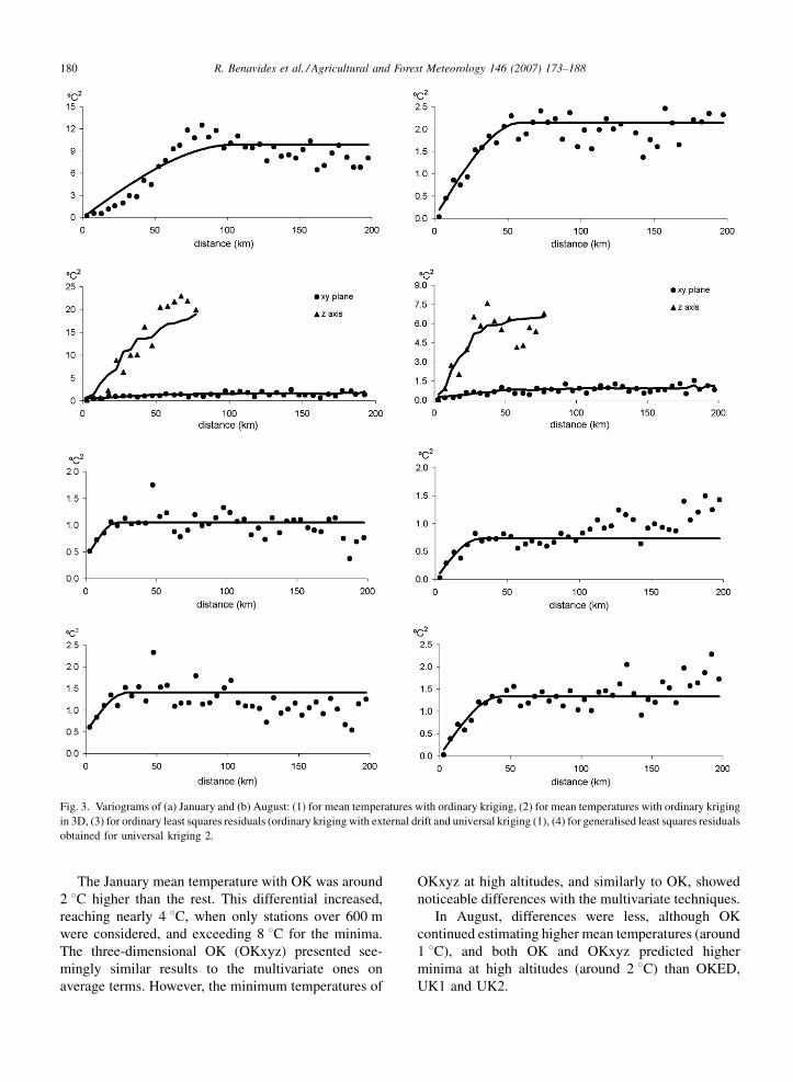
Fig. 3 shows the experimental variogram for the air

temperature and the spherical model fitted for OK, and

the directional variograms in the XY plane and Z-axis,

as well as the fitted spherical plus Gaussian model for

the OKxyz. The variogram for the OLS and the GLS

residuals and the fitted spherical models (for OKED

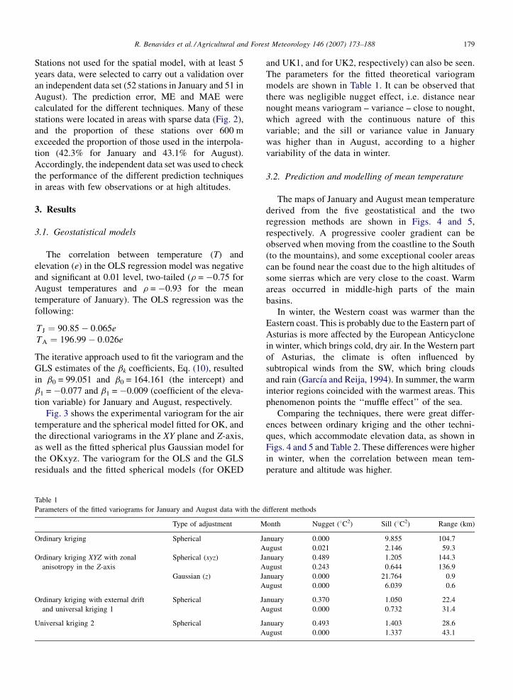
Table 1

Parameters of the fitted variograms for January and August data with the d

Type of adjustment M

Ordinary kriging Spherical J

A

Ordinary kriging XYZ with zonal

anisotropy in the Z-axis

Spherical (xyz) J

A

Gaussian (z) J

A

Ordinary kriging with external drift

and universal kriging 1

Spherical J

A

Universal kriging 2 Spherical J

A

and UK1, and for UK2, respectively) can also be seen.

The parameters for the fitted theoretical variogram

models are shown in Table 1. It can be observed that

there was negligible nugget effect, i.e. distance near

nought means variogram – variance – close to nought,

which agreed with the continuous nature of this

variable; and the sill or variance value in January

was higher than in August, according to a higher

variability of the data in winter.

3.2. Prediction and modelling of mean temperature

The maps of January and August mean temperature

derived from the five geostatistical and the two

regression methods are shown in Figs. 4 and 5,

respectively. A progressive cooler gradient can be

observed when moving from the coastline to the South

(to the mountains), and some exceptional cooler areas

can be found near the coast due to the high altitudes of

some sierras which are very close to the coast. Warm

areas occurred in middle-high parts of the main

basins.

In winter, the Western coast was warmer than the

Eastern coast. This is probably due to the Eastern part of

Asturias is more affected by the European Anticyclone

in winter, which brings cold, dry air. In the Western part

of Asturias, the climate is often influenced by

subtropical winds from the SW, which bring clouds

and rain (Garcıa and Reija, 1994). In summer, the warm

interior regions coincided with the warmest areas. This

phenomenon points the ‘‘muffle effect’’ of the sea.

Comparing the techniques, there were great differ-

ences between ordinary kriging and the other techni-

ques, which accommodate elevation data, as shown in

Figs. 4 and 5 and Table 2. These differences were higher

in winter, when the correlation between mean tem-

perature and altitude was higher.

ifferent methods

onth Nugget (8C2) Sill (8C2) Range (km)

anuary 0.000 9.855 104.7

ugust 0.021 2.146 59.3

anuary 0.489 1.205 144.3

ugust 0.243 0.644 136.9

anuary 0.000 21.764 0.9

ugust 0.000 6.039 0.6

anuary 0.370 1.050 22.4

ugust 0.000 0.732 31.4

anuary 0.493 1.403 28.6

ugust 0.000 1.337 43.1

R. Benavides et al. / Agricultural and Forest Meteorology 146 (2007) 173–188180

Fig. 3. Variograms of (a) January and (b) August: (1) for mean temperatures with ordinary kriging, (2) for mean temperatures with ordinary kriging

in 3D, (3) for ordinary least squares residuals (ordinary kriging with external drift and universal kriging (1), (4) for generalised least squares residuals

obtained for universal kriging 2.

The January mean temperature with OK was around

2 8C higher than the rest. This differential increased,

reaching nearly 4 8C, when only stations over 600 m

were considered, and exceeding 8 8C for the minima.

The three-dimensional OK (OKxyz) presented see-

mingly similar results to the multivariate ones on

average terms. However, the minimum temperatures of

OKxyz at high altitudes, and similarly to OK, showed

noticeable differences with the multivariate techniques.

In August, differences were less, although OK

continued estimating higher mean temperatures (around

1 8C), and both OK and OKxyz predicted higher

minima at high altitudes (around 2 8C) than OKED,

UK1 and UK2.

R. Benavides et al. / Agricultural and Forest Meteorology 146 (2007) 173–188 181

Table 2

Descriptive statistics of the predicted temperatures

January August

Stations

below 600 m

Stations equal

and over 600 m

All

stations

Stations

below 600 m

Stations equal

and over 600 m

All

stations

Ordinary kriging

Min (8C) 4.5 2.8 2.8 16.6 14.7 14.7

Max (8C) 10.0 9.3 10.0 20.6 20.5 20.6

Mean (8C) 8.1 6.1 7.1 19.0 18.6 18.8

S.D. (8C) 1.0 1.4 1.5 0.5 1.1 0.9

Ordinary kriging in 3D

Min (8C) 4.7 1.7 1.7 17.1 14.2 14.2

Max (8C) 9.4 7.5 9.4 20.2 18.7 20.2

Mean (8C) 7.5 3.6 5.7 18.8 16.4 17.7

S.D. (8C) 1.0 1.1 2.2 0.5 0.9 1.4

Ordinary kriging with external drift

Min (8C) 4.5 �6.7 �6.7 16.6 12.8 12.8

Max (8C) 9.9 6.5 9.9 20.6 19.8 20.6

Mean (8C) 7.3 2.7 5.1 18.9 17.2 18.1

S.D. (8C) 1.2 2.1 2.8 0.6 1.2 1.2

Universal kriging 1

Min (8C) 4.5 �6.3 �6.3 16.6 12.2 12.2

Max (8C) 9.9 6.7 9.9 20.6 19.7 20.6

Mean (8C) 7.3 2.8 5.2 18.9 17.0 18.0

S.D. (8C) 1.1 2.0 2.8 0.6 1.3 1.3

Universal kriging 2

Min (8C) 4.5 �6.1 �6.1 16.6 11.8 11.8

Max (8C) 9.9 6.7 9.9 20.6 19.6 20.6

Mean (8C) 7.3 2.9 5.2 18.8 16.9 17.9

S.D. (8C) 1.1 2.0 2.7 0.6 1.3 1.4

Regression model 1

Min (8C) 5.2 �5.1 �5.1 16.5 10.6 10.6

Max (8C) 9.4 5.7 9.4 20.0 18.1 20.0

Mean (8C) 7.3 3.0 5.3 18.3 16.0 17.3

S.D. (8C) 1.1 1.9 2.6 0.6 1.2 1.5

Regression model 2

Min (8C) 3.4 �5.0 �5.0 16.3 10.6 10.6

Max (8C) 10.3 8.0 10.3 21.0 19.9 21.0

Mean (8C) 7.3 3.3 5.4 18.6 16.4 17.6

S.D. (8C) 1.1 1.9 2.5 0.6 1.2 1.5

The first regression model is the one developed by Sanchez-Palomares et al. (1999) and the second one is the model developed by Ninyerola et al.

(2005).

The regression models estimated mean temperatures

similar to those of the multivariate spatial models in

January, although the minimum temperatures were

smoothed. In August, the regression models gave

slightly lower mean and minimum temperatures than

the multivariate spatial models.

3.3. Validation and kriging error distribution

Table 3 shows the NME and NRMSE resulting from

the cross-validation for the OK, OKxyz, OKED, UK1

and UK2 methods. The NME was approximately 0 for

every kriging technique, which indicated that air

R. Benavides et al. / Agricultural and Forest Meteorology 146 (2007) 173–188182

Fig. 4. Models of predicted mean air temperature in January: (a) ordinary kriging, (b) ordinary kriging in 3D, (c) ordinary kriging with external drift,

(d) universal kriging 1, (e) universal kriging 2, (f) Sanchez-Palomares’ regression model, (g) Ninyerola’s regression model.

Fig. 5. Models of predicted mean air temperature in August: (a) ordinary kriging, (b) ordinary kriging in 3D, (c) Ordinary kriging with external drift,

(d) universal kriging 1, (e) universal kriging 2, (f) Sanchez-Palomares’ regression model, (g) Ninyerola’s regression model.

Table 3

Normalised mean error (NME) and normalised root mean squared error (NRMSE) of the values inferred by cross-validation, for each technique (OK:

ordinary kriging; OKxyz: ordinary kriging in 3D; OKED: ordinary kriging with external drift, UK: universal kriging), and during January and

August

January August

OK OKxyz OKED UK1 UK2 OK OKxyz OKED UK1 UK2

NME 0.025 0.003 0.017 0.011 0.009 0.016 0.008 0.028 0.030 0.026

NRMSE 0.737 0.320 0.994 0.996 0.875 1.190 1.136 1.181 1.156 0.955

R. Benavides et al. / Agricultural and Forest Meteorology 146 (2007) 173–188 183

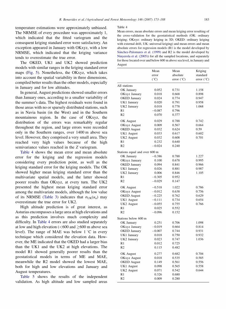
Table 4

Mean errors, mean absolute errors and mean kriging error resulting of

the cross-validation for the geostatistical methods (OK: ordinary

kriging; OKxyz: ordinary kriging in 3D; OKED: ordinary kriging

with external drift, UK: universal kriging) and mean errors and mean

absolute errors for regression models (R1 is the model developed by

Sanchez-Palomares et al. (1999) and R2 is the model developed by

Ninyerola et al. (2005)) for all the sampled locations, and separately

for those located over and below 600 m above sea level, in January and

August

Mean

error

(8C)

Mean

absolute

error (8C)

Kriging

standard

error (8C)

All stations

OK January 0.052 0.731 1.158

OKxyz January 0.018 0.668 0.898

OKED January 0.024 0.774 0.947

UK1 January 0.020 0.791 0.958

UK2 January 0.018 0.778 1.068

R1 �0.087 0.796

R2 0.070 0.377

OK August 0.029 0.788 0.742

OKxyz August 0.009 0.567 0.664

OKED August 0.032 0.624 0.59

UK1 August 0.033 0.617 0.602

UK2 August 0.032 0.608 0.701

R1 0.232 0.640

R2 �0.024 0.240

Stations equal and over 600 m

OK January �0.386 0.788 1.227

OKxyz January 0.100 0.678 0.995

OKED January 0.094 0.841 0.966

UK1 January 0.026 0.881 0.987

UK2 January 0.006 0.846 1.105

R1 �0.305 0.952

R2 �0.029 0.147

OK August �0.518 1.022 0.786

OKxyz August �0.012 0.638 0.756

OKED August �0.225 0.762 0.629

UK1 August �0.111 0.734 0.654

UK2 August �0.055 0.755 0.766

R1 0.025 0.552

R2 �0.096 0.152

Stations below 600 m

OK January 0.251 0.706 1.098

OKxyz January �0.019 0.664 0.814

OKED January �0.007 0.744 0.931

UK1 January 0.018 0.750 0.932

UK2 January 0.023 0.747 1.036

R1 0.012 0.725

R2 0.115 0.482

OK August 0.277 0.682 0.704

OKxyz August 0.018 0.535 0.585

OKED August 0.149 0.561 0.556

UK1 August 0.098 0.565 0.558

UK2 August 0.071 0.542 0.644

R1 0.326 0.680

R2 0.009 0.280

temperature estimations were approximately unbiased.

The NRMSE of every procedure was approximately 1,

which indicated that the fitted variogram and the

consequent kriging standard error were satisfactory. An

exception appeared in January with OKxyz, with a low

NRMSE, which indicated that the kriging variance

tends to overestimate the true error.

The OKED, UK1 and UK2 showed prediction

models with similar ranges in the kriging standard error

maps (Fig. 5). Nonetheless, the OKxyz, which takes

into account the spatial variability in three dimensions,

compiled better results than the other models, especially

in January and for low altitudes.

In general, August predictions showed smaller errors

than January ones, according to a smaller variability of

the summer’s data. The highest residuals were found in

those areas with no or sparsely distributed stations, such

as in Navia basin (in the West) and in the Southern

mountainous region. In the case of OKxyz, the

distribution of the errors was remarkably regular

throughout the region, and large errors were recorded

only in the Southern ranges, over 1400 m above sea

level. However, they comprised a very small area. They

reached very high values because of the high

semivariance values reached in the Z variogram.

Table 4 shows the mean error and mean absolute

error for the kriging and the regression models

considering every prediction point, as well as the

kriging standard error for the kriging models. The OK

showed higher mean kriging standard error than the

multivariate spatial models, and the latter showed

poorer results than OKxyz, at every turn. The UK2

presented the highest mean kriging standard error

among the multivariate models, although the low value

of its NRMSE (Table 3) indicates that sUK(ua) may

overestimate the true error for UK2.

High altitude prediction is of great interest, as

Asturias encompasses a large area at high elevations and

as this prediction involves much complexity and

difficulty. In Table 4 errors are also studied separately

at low and high elevation (<600 and �600 m above sea

level). The range of MAE was below 1 8C in every

technique which considered the elevation data. How-

ever, the ME indicated that the OKED had a larger bias

than the UK1 and the UK2 at high elevations. The

model R1 showed generally poorer results than the

geostatistical models in terms of ME and MAE,

meanwhile the R2 model showed the lowest MAE,

both for high and low elevations and January and

August temperatures.

Table 5 shows the results of the independent

validation. As high altitude and low sampled areas

R. Benavides et al. / Agricultural and Forest Meteorology 146 (2007) 173–188184

Table 5

Mean temperature, mean errors (ME), mean absolute errors (MAE), kriging standard error estimates (s), normalised mean error (NME) and

normalised root mean squared error (NRMSE) for the independent validation data set (OK: ordinary kriging; OKxyz: ordinary kriging in 3D; OKED:

ordinary kriging with external drift, UK: universal kriging, R1 is the model developed by Sanchez-Palomares et al. (1999) and R2 is the model

developed by Ninyerola et al. (2005)), in January and August

Temperature (8C) ME (8C) MAE (8C) s (8C) NME NRMSE

January

OK 6.3 �0.373 1.049 1.277 �0.276 1.283

OKxyz 5.7 0.178 0.863 0.835 0.119 1.124

OKED 5.8 0.120 0.866 0.953 0.104 1.116

UK1 5.8 0.107 0.862 0.959 0.064 1.119

UK2 5.8 0.074 0.856 1.076 0.183 1.118

R1 5.8 0.051 0.831

R2 5.7 0.188 0.867

August

OK 18.6 �0.348 1.041 0.830 �0.460 1.857

OKxyz 18.3 �0.082 0.771 0.428 �0.204 1.070

OKED 18.5 �0.244 0.897 0.649 �0.456 1.218

UK1 18.4 �0.213 0.888 0.652 �0.413 1.215

UK2 18.4 �0.197 0.884 0.768 �0.335 1.198

R1 18.1 0.146 0.879

R2 18.1 0.100 0.753

were relatively more frequent in the data set used for the

independent validation, the mean estimated tempera-

tures were lower than for the entire study area, and the

errors and biases were higher than for the cross-

validation. However, the MAE was smaller than 1 8Cfor all the interpolation techniques except for OK. The

R1 regression model showed smaller bias and MAE in

January than the other techniques, whereas the OKxyz

and R2 were the techniques which performed better in

August. It was remarkable that the difference between

the MAE made with R2 and the rest of techniques

disappeared. Even in January, we can see that R2

presented poorer results that the geostatistical perfor-

mances.

4. Discussion

Geostatistical techniques have been used to infer

reasonable models, from accuracy and time-capacity

computing points of view, of the mean air temperature

in January and August. Air temperature is one of the

main external factors affecting ecological processes.

The three analysed geostatistical methods that included

elevation as an auxiliary variable to estimate the

distribution of mean monthly air temperature, showed

similar patterns with reasonable estimation errors, as

well as error estimations, which indicates the adequacy

of the spatial models developed. Furthermore, a new

approach based on XYZ kriging with zonal anisotropy in

the Z direction has been applied with promising results.

The absence of an underlying deterministic relationship

between elevation and temperature constitutes the main

difference between this approach and the multivariate

geostatistical techniques and the regression models

analysed.

August predictions had generally smaller errors than

in January. This is in accordance with the higher

variability in January data and the higher variances

found in January variograms. This is similar to the trend

found by Rolland (2002), where the air temperature

interpolation error was higher in January than in July

(the warmest month in its study region). As previously

reported (Hudson and Wackernagel, 1994; Dodson and

Marks, 1997), correlations between temperature and

elevation may change seasonally, and were higher in

this study in January than in August. A similar trend

appeared in Israel (Kurtzman and Kadmon, 1999)

where the regression coefficient between the January

mean daily temperature and altitude reached R2 = 0.84,

meanwhile with June temperatures this coefficient was

R2 = 0.57. Besides, in Scotland (Hudson and Wack-

ernagel, 1994), mean temperature of July held the

weakest correlation coefficient with elevation of every

studied month (January, April, July and October),

because of the strong correlation with latitude in

summer.

Taking into account these correlation coefficients, it

is not surprising that the models inferred with the

elevation data brought about more accurate predictions,

because altitude plays a major part in climatic spatial

R. Benavides et al. / Agricultural and Forest Meteorology 146 (2007) 173–188 185

Fig. 6. Maps of the kriging (prediction) standard errors: (1) January, (2) August. (a) Ordinary kriging, (b) ordinary kriging in 3D, (c) ordinary kriging

with external drift, (d) universal kriging 1, (e) universal kriging 2.

changes in mountainous areas (Stoutjesdijk and Bark-

man, 1992). OKxyz, UKs and OKED improved the

temperature estimations made with OK. In Fig. 6 and in

Table 4, the kriging errors and mean errors at sampled

locations decreased when elevation was considered (on

average 15% in kriging error terms). This improvement

was greater in winter time (January) at high elevations

(�600 m). Recall that January temperatures showed

higher correlation with altitude data.

The impressive differences in the prediction maps

and the prediction errors between the OK and OKxyz

techniques show the importance of the variogram model

in the kriging prediction. In fact, the only difference

between both approaches was the variogram computing

method. With OKxyz, the kriging weights were

drastically reduced when the altitude difference

increased. Surprisingly, the prediction maps derived

through OKxyz were very similar to those derived from

the OKED, UK1, UK2 and the regression models,

which assumed a deterministic linear relationship

between temperature and elevation. However, the

highest point prediction errors were recorded with

the seemingly more accurate geostatistical technique,

the OKxyz, with figures around 5 8C in January, and

nearly 3 8C in August. In Fig. 6 these large prediction

errors encompassed a small area with only 6.7%

(January) and 4.8% (August) of the surface exceeding

the prediction error by 1 8C. Moreover, they matched up

with the highest elevations (over 1400 m), due to the

high altitude differences between the nearest stations.

UK2 showed larger kriging errors than the other

multivariate kriging methods (1.4 8C for both months),

which is in accordance with the highest variogram sill

value (Table 1). Nevertheless, sUK(ua) for UK2 may be

a more reliable estimator of the true kriging variance, as

the NRSME indicates. In fact, the variogram estimate

based on the OLS residuals had larger bias than the

estimate based on the GLS residuals (Cressie, 1993).

Conversely, although the OKED and the UK1

techniques were based on the residuals of the same

regression model, the UK1 included the elevation of the

prediction points and the sampled points in the kriging

system. Hence, UK1 must give more precise predicted

error estimates (as the NME and the NRMSE indicate)

than OKED, which does not incorporate the uncertainty

within the internal model.

R. Benavides et al. / Agricultural and Forest Meteorology 146 (2007) 173–188186

For stations at altitudes above 600 m, the MAE with

OK was similar to the MAE with OKED, UK1 and

UK2, but the ME indicated that OK estimates were

strongly biased towards higher temperatures (Tables 4

and 5), probably because of the non-homogeneous

altitudinal distribution of the stations. The inclusion of

the variability on the Z direction in the OKxyz seemed

to solve the bias problem, and this approach held the

best results in terms of MAE in both months. For the

high altitude stations, the UK2 showed a smaller bias,

specially in January, when the correlation between

elevation and temperature was higher. Conversely, the

OKED showed larger bias (mean error) than the other

multivariate kriging methods, towards lower tempera-

tures in January, and specially towards higher tempera-

tures in August, when the correlation between elevation

and temperature is lower. In fact, for August, the

absolute value of the coefficient in the regression model

was quite low, so the regression may overestimate high

altitude temperatures, whereas the ordinary kriging may

smooth the residuals at these altitudes. In January, it

seems to occur conversely. The biased August

temperature estimations with OKED were also corro-

borated by the independent validation.

The regression model with elevation as a unique

independent variable showed a strong bias towards low

temperatures at low altitudes in August and towards

high temperatures at high altitudes in January,

smoothing the extreme temperature values. The

decrease in efficiency of simple regression analysis

for assessing temperature with elevation was also

confirmed by Rolland (2002). The model developed by

Ninyerola et al. (2005), which included other variables

such as the distance to the sea or the curvature radius of

the terrain, showed much better performance in bias

terms and was the most precise in MAE terms,

particularly at higher elevations where MAE was under

0.16 8C for both months. Nonetheless, the R2 model

gave more biased estimations than OKxyz and UK2,

and its implementation was more complex than the rest

as it requires a solar radiance model and some GIS

development to derive the independent variables.

Surprisingly, the independent validation, that mainly

reflects the model’s performance in poorly sampled

areas, did not show better results for the regression

models than for the kriging techniques. In fact, all the

techniques except OK gave similar figures in terms of

MAE. When accounting for the bias, the UK2 and R1

techniques showed slightly better results in January,

when the correlation between elevation and temperature

was higher, whereas in August the OKxyz and R2

regression model gave the best results.

5. Conclusions

In spite of the scarce and irregularly distributed

number of sampled data, the models derived from

geostatistical techniques with elevation as an auxiliary

variable were quite accurate, especially the ordinary

kriging XYZ with zonal anisotropy in the Z direction.

The variogram fitting procedure of the OKxyz has been

developed in the frame of this research, and with the

same independent variables (UTM-coordinates and

elevation data) improved the regression models. These

techniques were satisfactory, since other predictive

models had lower predictive power (OK and R1) or they

mean a complex analysis such as R2, which required

technical resources that are not always available, and

more time and computing-capacity. Also, it has been

shown that predictions with R2 in places elsewhere do

not necessarily provide the best results. Future

directions of this research include the use of other

variables in the multivariate kriging methods, continu-

ing the trend followed by regression techniques, and the

use of geostatistical techniques to study the temporal

variability of ecological variables, a key aspect for

every natural resources management.

Acknowledgements

We want to thank Miguel Angel Alvarez, Director of

the Instituto de Recursos Naturales y Ordenacion del

Territorio (INDUROT), Asturias, for supplying the

temperature data set. We are also grateful to Dr. Grant

Douglas, Dr. Sonia Roig and Rocio Rosa for their

valuable comments on the manuscript. The research

was supported by a fellowship awarded to R. Benavides

from the Ministry of Education and Science of Spain, in

the context of project AGL2003-05342.

References

Ayalew, L., Reik, G., Busch, W., 2002. Characterizing weathered rock

masses—a geostatistical approach. Int. J. Rock Mech. Min. Sci.

39, 105–114.

Barry, R.G., Chorley, R.J., 1987. Atmosphere, Weather and Climate,

fifth ed. Methuen and Co., London, 459 pp.

Blennow, K., 1993. Frost in July in a coastal area of southern Sweden.

Weather 48, 217–222.

Blennow, K., 1998. Modelling minimum air temperature in par-

tially and clear felled forest. Agric. Forest Meteorol. 91, 223–

235.

Carrega, P., 1995. A method for reconstruction of mountain air

temperatures with automatic cartographic applications. Theor.

Appl. Climatol. 52, 69–84.

Cressie, N.A.C., 1993. Statistics for Spatial Data. Wiley, New York,

900 pp.

R. Benavides et al. / Agricultural and Forest Meteorology 146 (2007) 173–188 187

De Iaco, S., Myers, D.E., Posa, D., 2002. Nonseparable space-time

covariance models: some parametric families. Math. Geol. 34,

23–42.

De Phillips, A., 1951. Forest ecology and phytoclimatology (on line)

Unasylva 5 (1), available in: http://www.fao.org/documents/

show_cdr.asp?url_file=/docrep/x5358e/x5358e03.htm (Con-

sulted: March 2006).

del Valle, S., 2004. Determinacion con base ecologica de la Pro-

ductividad Potencial Forestal in la provincia de Santiago de

Estero, Argentina (Determination of the potential forest produc-

tivity in the province of Santiago de Estero, Argentina, with

ecological basis). Doctoral Thesis, Universidad Politecnica de

Madrid.

Dodson, R., Marks, D., 1997. Daily air temperature interpolated at

high spatial resolution over a large mountainous region. Climate

Res. 8, 1–20.

Fliri, F., 1975. Das Klima der Alpen in Raume von Tirol, Mono-

graphien zur Landskunde Tirols (The climate of the Alps in the

Tirol area. Monographics of Tirol geography). Folgen, Universitat

Wagner, Innsbruck, Munchen, 454 pp.

Gafta, D., Pedrotti, F., 1996. Fitoclima del Trentino-Alto-Adige

Sudtirol studi Trentini di scienze naturali (Phitoclimate of the

Trentino-Alto-South Tirol. Trentini studies of Natural Sciences).

Acta Biol 73, 55–100.

Gandullo, J.M., 1994. Climatologıa y ciencias del suelo (Climatology

and Soil Sciences). Fundacion Conde del Valle Salazar, ETSI

Montes, Madrid, 408 pp.

Garcıa, L., Reija, A., 1994. Tiempo y clima en Espana. Meteorologıa

de las Comunidades Autonomas (Weather and climate in Spain:

meteorology of the different autonomous communities). Dossat-

2000, Madrid, 410 pp.

Geisser, S., 1975. The predictive simple rause method with applica-

tions. J. Am. Stat. Assoc. 70, 320–328.

Goodale, C.L., Albert, J.D., Ollinger, S.V., 1998. Mapping monthly

precipitation, temperature and solar radiation for Ireland with

polynomial regression and digital elevation model. Climate

Res. 10, 35–49.

Goovaerts, P., 1999. Geostatistics in soil science: state-of-the-art and

perspectives. Geoderma 89, 1–45.

Gringarten, E., Deutsch, C.V., 2001. Variogram interpretation and

modeling. Math. Geol. 33, 507–534.

Hagglund, B., 1981. Evaluation of forest site productivity. Forest

Abstr. 42 (11), 515–527 (review article).

Hayhoe, H.N., Lapen, D.R., 2001. Spatially modelling temperature

normals in the Rocky Mountains with kriging and cokriging

estimators using ANN produced secondary information. In:

Proceedings II Conference of Artificial Intelligence, AMS, Annual

Meeting, Long Beach, CA.

Hudson, G., Wackernagel, H., 1994. Mapping temperature using

kriging with external drift: theory and example from Scotland.

Int. J. Climatol. 14, 77–91.

Isaaks, E.H., Srivastava, R.M., 1989. Applied Geostatistics. Oxford

University Press, New York, 561 pp.

Ishida, T., Kawashima, S., 1993. Use of cokriging to estimate surface

air temperature from elevation. Theor. Appl. Climatol. 47, 147–

157.

Kurtzman, D., Kadmon, R., 1999. Mapping of temperature variables

in Israel: a comparison of different interpolation methods. Climate

Res. 13, 33–43.

Lapen, D.R., Hayhoe, H.N., 2003. Spatial analysis of seasonal and

annual temperature and precipitations normals in Southern

Ontario, Canada. J. Great Lakes Res. 29 (4), 529–544.

Li, X., Cheng, G., Lu, L., 2005. Spatial analysis of air temperature in

Qinghai-Tibet Plateau. Arctic Antarct. Alpine Res. 37 (2), 246–

252.

Lutgens, F.K., Tarbuck, E.J., 1995. The Atmosphere: An Introduction

to Meteorology, sixth ed. Prentice-Hall, Englewood Cliffs, NJ,

462 pp.

Marquınez, J., Lastra, J., Garcıa, P., 2003. Estimation models for

precipitation in mountainous regions: the use of GIS and multi-

variate analysis. J. Hydrol. 270, 1–11.

Montes, F., Hernandez, M.J., Canellas, I., 2005. A geostatistical

approach to cork production sampling estimation in Quercus suber

forests. Can. J. Forest Res. 35, 2787–2796.

Myers, D.E., Journel, A., 1990. Variograms with zonal anisotropies

and non-invertible kriging systems. Math. Geol. 22, 779–785.

Nalder, I.A., Ross, W.W., 1998. Spatial interpolation of climatic

normals: test of a new method in Canadian boreal forest. Agric.

Forest Meteorol. 92, 211–225.

Neuman, S.P., Jacobson, E.A., 1984. Analysis of nonintrinsic spatial

variability by residual kriging with application to regional ground-

water levels. J. Int. Assoc. Math. Geol. 16, 499–521.

Ninyerola, M., Pons, X., Roure, J.M., 2000. A methodological

approach of climatological modelling of air temperature and pre-

cipitation through GIS techniques. Int. J. Climatol. 20, 1823–1841.

Ninyerola, M., Pons, X., Roure, J.M., 2005. Atlas climatico digital de

la Penınsula Iberica. Metodologıa y Aplicaciones en bioclimato-

logıa y geobotanica (Digital Climatic Atlas of the Iberian Penin-

sula. Methodology and Implementations in Bioclimatology and

Geobotanic) (on line) ISBN 932860-8-7. Universidad Autonoma

of Barcelona. Besllaterra. Available in: http://opengis.uab.es/wms/

iberia/mms/index.htm (Consulted: April 2006).

Richardson, A.D., Lee, X., Friedland, A.J., 2004. Microclimatology of

treeline spruce-fir forests in mountains of the northeastern United

States. Agric. Forest Meteorol. 125, 53–66.

Robeson, S.M., 1994. Influence of spatial interpolation and sampling

on estimates of terrestrial air temperature change. Climate Res. 4

(2), 119–126.

Rolland, C., 2002. Spatial and seasonal variations of air temperature

lapse rate in Alpine region. J. Climate (Am. Meteorol. Soc.) 16 (7),

1032–1046.

Rouhani, S., Myers, D.E., 1990. Problems in space-time kriging of

geohydrological data. Math. Geol. 22, 611–623.

Rubio, A., Sanchez, O., Gomez, V., Grana, D., Elena, R., Blanco, A.,

2002. Autoecologıa de los castanares de Castilla (Espana) (Auto-

ecology of chestnut tree forest in Castilla, Spain). Investigacion

Agraria: Sistemas de Recursos Forestales 11 (2), 373–393.

SADEI (Sociedad Asturiana de Estudios Economicos e Industriales),

2005. Superficie de Asturias segun estratos de pendiente

(Surface area of Asturias according to slopes ranges). Based on

the National Geographic Institute’s Source (on line), available in:

http://www.sadei.es/datos/cuadros%20tematicos/capitulo%20A/

4/A40004XXXXXa.xls (Consulted: August 2006).

Sanchez-Palomares, O., Sanchez-Serrano, F., Carretero, M. P., 1999.

Modelos y Cartografıa de estimaciones climaticas termopluvio-

metricas para la Espana peninsular (Models and Maps of the

climatic variables estimates in peninsular Spain). Ministerio de

Agricultura, Pesca y Alimentacion. Instituto Nacional de Inves-

tigacion y Tecnologıa Agraria y Alimentaria, Madrid, 192 pp.

Sanchez-Palomares, O., Rubio, A., Blanco, A., Elena, R., Gomez, V.,

2003. Autoecologıa parametrica de los hayedos de Castilla y Leon

(Parametric Autoecology of beech tree forest in Castilla y Leon).

Investigacion Agraria: Sistemas de Recursos Forestales 12 (1),

87–110.

R. Benavides et al. / Agricultural and Forest Meteorology 146 (2007) 173–188188

Serrada, R., 1976. Metodo para la evaluacion con base ecologica de la

productividad potencial de las masas forestales en grandes

regiones y su aplicacion a la Espana Peninsular (Methodology

for assessing the potential productivity of forest in large regions

and its application in peninsular Spain). Doctoral Thesis, Uni-

versidad Politecnica of Madrid.

Stone, M., 1974. Cross-validation choice and assessment of statistical

predictions. J. Royal Stat. Soc. B 36, 111–133.

Stoutjesdijk, P., Barkman, J.J., 1992. Microclimate, Vegetation and

Fauna. Opulus Press, Sweden, 216 pp.

Thom, H.C.S., 1966. Some Methods of Climatology Analysis.

W.O.M., 415, Technical Report 81, Geneve.