Getting Started with Excel 2000/2001/XP/Xexphysio/mvs110l/excel2000_XP.pdf · Getting Started with Excel 2000/2001/XP/X A Workshop Overview Excel is an excellent tool for data storage

Getting Started with Excel 2000/2001/XP/X A Workshop

Overview ........................................................................................................................ 2

Resizing Columns and Rows ....................................................................................... 3

Using the AutoFill Command ....................................................................................... 3

Using Formulas and Functions.................................................................................... 4 Using the AutoSum Command ................................................................................................... 4 Using the Paste Function Command........................................................................................... 5

Creating Charts ............................................................................................................. 6 Step 1: Chart Type ...................................................................................................................... 6 Step 2: Chart Source Data........................................................................................................... 6 Step 3: Chart Options.................................................................................................................. 7 Step 4: Chart Location ................................................................................................................ 7

Modifying Your Chart in Excel ..................................................................................... 8 Chart Menu ................................................................................................................................. 8 Double-Clicking Elements.......................................................................................................... 8 Chart Toolbar.............................................................................................................................. 8

Creating Overlapping Charts in Excel ......................................................................... 9 Creating a Custom Chart Type ................................................................................................... 9 Using the Paste Special Command ............................................................................................. 9

Formatting ................................................................................................................... 10 Formatting Cells ....................................................................................................................... 10 Formatting the Page .................................................................................................................. 10

Using Panes to Create Spreadsheet Headers........................................................... 10

Weighted Averages ..................................................................................................... 11 Defining a Named Area ............................................................................................................ 11 Substituting Letter Grades ........................................................................................................ 12

The Faculty Exploratory is located on the second floor of the Harlan Hatcher Graduate Library. [email protected] | http://www.lib.umich.edu/exploratory | (734) 647-7406.

rev: 5/23/03 1 of 12


Overview Excel is an excellent tool for data storage and analysis, whether it is for students’ information or statistical data for research. An Excel worksheet is made up of a series of columns (named with letters e.g. A, B, C…) and rows (named with numbers e.g. 1, 2, 3…), forming the cells.

When you open Excel, a blank workbook is automatically opened. A workbook is a file with one or more sheets; each worksheet is a “page” in the workbook where you enter and work with your data. Each workbook starts with three sheets, but you may add more sheets by going to the Insert menu option, then Worksheet. Each worksheet has a name tab at the lower left corner of the window, as shown below. To change the name of the worksheet double click on the tab, and then type the new name.

The term spreadsheet is a generic term for a worksheet.

To enter data, just click on the appropriate cell and start typing. When you type, the data goes into the currently selected cell, called the active cell. All the data you enter in the active cell appear on the formula bar. If you need to change the data, you can double-click on the cell to activate the cursor in the cell, or click in the formula bar and make the change there.

Formula bar

Worksheet’s name

Column headings

Active Cell

Row headings

Selection reference (column and row) displayed in the Name box

A tip that may help you to enter data more quickly is to use the Enter (Return on the Mac) and Tab keys to move from cell to cell. Enter (Return on the Mac) accepts your entry and moves the active cell down one, and the Tab accepts your entry and moves the active cell to the right. You can also use the arrow keys on the keyboard to move around the worksheet.

The Esc key or red X in the formula bar will abort your change.


rev: 5/23/03 2 of 12


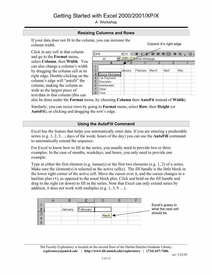
Resizing Columns and Rows If your data does not fit in the column, you can increase the column width. Column A’s right edge

Click in any cell in that column and go to the Format menu, select Column, then Width. You can also change a column’s width by dragging the column cell at its right edge. Double-clicking on the column’s edge will “autofit” the column, making the column as wide as the largest piece of text/data in that column (this can also be done under the Format menu, by choosing Column then AutoFit instead of Width).

Similarly, you can resize rows by going to Format menu, select Row, then Height (or AutoFit), or clicking and dragging the row’s edge.

Using the AutoFill Command Excel has the feature that helps you automatically enter data. If you are entering a predictable series (e.g. 1, 2, 3…; days of the week; hours of the day) you can use the AutoFill command to automatically extend the sequence.

For Excel to know how to fill in the series, you usually need to provide two or three examples. In the case of months, weekdays, and hours, you only need to provide one example.

Type in either the first element (e.g. January) or the first two elements (e.g. 1, 2) of a series. Make sure the element(s) is selected as the active cell(s). The fill handle is the little block in the lower right corner of the active cell. Move the cursor over it, and the cursor changes to a hairline plus (+), as opposed to the usual block plus. Click and hold on the fill handle and drag to the right (or down) to fill in the series. Note that Excel can only extend series by addition, it does not work with multiples (e.g. 1, 3, 9 …).

Excel’s guess to what the next cell should be.


rev: 5/23/03 3 of 12


Using Formulas and Functions Formulas in Excel are useful to perform various mathematical, statistical, and logical operations. You can type in a formula (though you have to be sure it’s exactly right) or you can use Excel’s preset formulas called functions. Excel can perform simple tasks like a calculator; for example, if you typed in =5*6 then pushed Enter/Return on the keyboard, what would appear in the cell would be 30. If you selected the cell again, though, you would see the formula =5*6. If you type in the formula, you must start with an equal sign, so Excel knows that the data in the cell is a formula. After the =, what comes next depends on what you’re trying to do. If you are multiplying numbers (like in the above example), you would just type in the appropriate numbers and mathematical symbol (* for multiply).

The power of Excel, however, is to do more complicated calculations, including calculations for the cell itself, no matter what the content (meaning, if the content of the cell changes from a 5 to a 6, for example) and more complex formulas (such as averages, sums, etc., beyond basic math). Just like a basic formula, you need to start with the equal sign. After that, you would put the function name, then the range of cells inside parentheses. For example: =SUM(B2:B5)

Using the AutoSum Command

Since sum is used so frequently in Excel, there is an icon on the toolbar for it. When you use the AutoSum command, Excel guesses what data you want to enter (usually a block of cells next to the cell where the formula is). To use the AutoSum, go to the cell where you want the summation result to appear, click on the AutoSum icon and verify if Excel’s guess is correct. If it is not correct, select the cells you wish to add to the formula by clicking on the first cell and dragging to the last one. Then press Enter/Return on the keyboard. The sum of the data of the selected range of cells will appear in the cell with the formula. If any of the values in this range of cells are changed, the cell with the summation formula will automatically update to reflect the new sum.

The AutoSum button is located on the Standard Toolbar


rev: 5/23/03 4 of 12


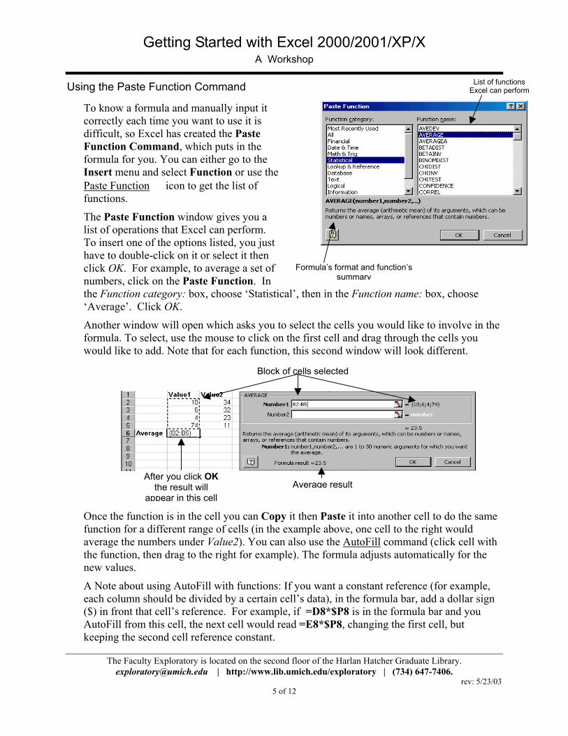
List of functions Excel can performUsing the Paste Function Command

To know a formula and manually input it correctly each time you want to use it is difficult, so Excel has created the Paste Function Command, which puts in the formula for you. You can either go to the Insert menu and select Function or use the Paste Function icon to get the list of functions.

Formula’s format and function’s summary

The Paste Function window gives you a list of operations that Excel can perform. To insert one of the options listed, you just have to double-click on it or select it then click OK. For example, to average a set of numbers, click on the Paste Function. In the Function category: box, choose ‘Statistical’, then in the Function name: box, choose ‘Average’. Click OK.

Another window will open which asks you to select the cells you would like to involve in the formula. To select, use the mouse to click on the first cell and drag through the cells you would like to add. Note that for each function, this second window will look different.

After you click OK the result will

appear in this cell Average result

Block of cells selected

Once the function is in the cell you can Copy it then Paste it into another cell to do the same function for a different range of cells (in the example above, one cell to the right would average the numbers under Value2). You can also use the AutoFill command (click cell with the function, then drag to the right for example). The formula adjusts automatically for the new values.

A Note about using AutoFill with functions: If you want a constant reference (for example, each column should be divided by a certain cell’s data), in the formula bar, add a dollar sign ($) in front that cell’s reference. For example, if =D8*$P8 is in the formula bar and you AutoFill from this cell, the next cell would read =E8*$P8, changing the first cell, but keeping the second cell reference constant.


rev: 5/23/03 5 of 12


Creating Charts To insert a Chart, go to the Insert menu, and then click on Chart… or click on the Chart Wizard icon ( ) in the toolbar. A Chart Wizard window will pop up and guide you through the creation of your chart.

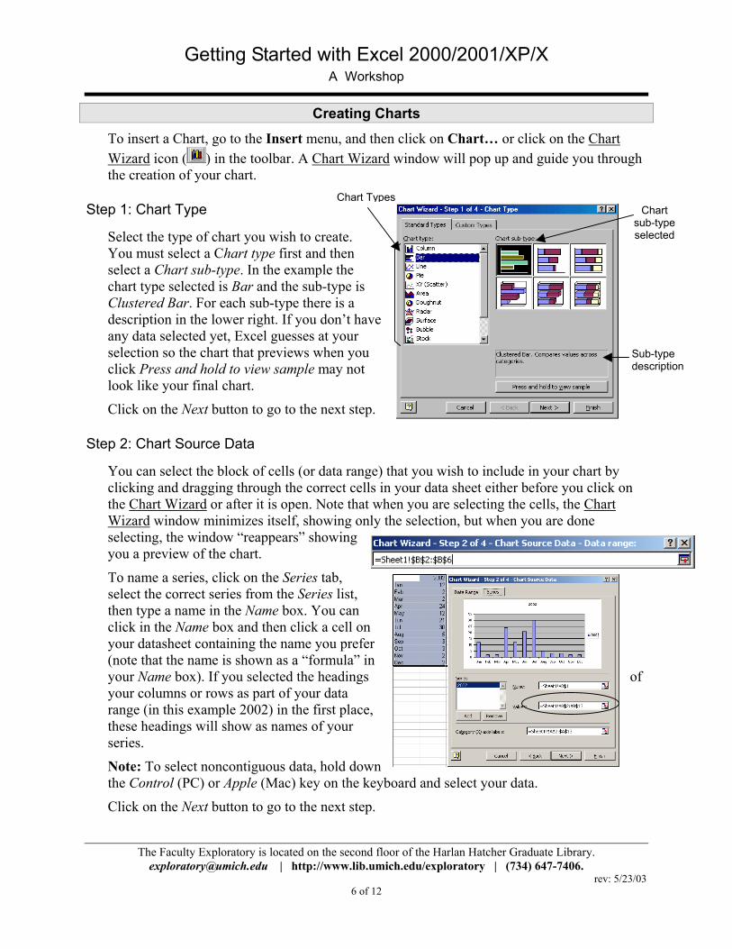
Chart TypesStep 1: Chart Type Chart

sub-type selected Select the type of chart you wish to create.

You must select a Chart type first and then select a Chart sub-type. In the example the chart type selected is Bar and the sub-type is Clustered Bar. For each sub-type there is a description in the lower right. If you don’t have any data selected yet, Excel guesses at your selection so the chart that previews wh n you click Press and hold to view sample m not look like your final chart.

Sub-type description

Click on the Next button to go to the ne

Step 2: Chart Source Data

You can select the block of cells (or daclicking and dragging through the corrthe Chart Wizard or after it is open. NoWizard window minimizes itself, showselecting, the window “reappears” shoyou a preview of the chart.

To name a series, click on the Series taselect the correct series from the Seriesthen type a name in the Name box. Yoclick in the Name box and then click ayour datasheet containing the name yo(note that the name is shown as a “formyour Name box). If you selected the heyour columns or rows as part of your drange (in this example 2002) in the firsthese headings will show as names of yseries.

Note: To select noncontiguous data, hothe Control (PC) or Apple (Mac) key o

Click on the Next button to go to the ne

The Faculty Exploratory is located on [email protected] | http://w

eay

xt step.

ta range) that you wish to include in your chart by ect cells in your data sheet either before you click on te that when you are selecting the cells, the Chart ing only the selection, but when you are done

wing

b, list,

u can cell on u prefer ula” in

adings of ata t place, our

ld down n the keyboard and select your data.

xt step.

e second floor of the Harlan Hatcher Graduate Library. ww.lib.umich.edu/exploratory | (734) 647-7406.

rev: 5/23/03 6 of 12


Step 3: Chart Options

There are six tabs with different formatting options. Note that a preview of your graph with the format changes is shown on the right side of this window.

• Titles: Add a title to your chart, and to either axis. These will display in the preview window

• Axes: Show or hide the values of either axis and format the values for the x-axis.

• Gridlines: Show or hide gridlines for both axes. Preview

• Legend: Show or hide the legend, and decide placement. In this preview, the legend is at the right of the chart.

• Data Labels: Show exact values in your chart from either axis.

• Data Table: Show your data along with the chart.

Go through all the tabs, and add/remove options to show the chart the way you want it. When you are finished, click on the Next button to go to the next step. Once you’ve created the chart, remember you can always come back and change anything by selecting the chart then going to the Chart menu and then Chart Options….

Step 4: Chart Location

Your chart can be inserted as an object in the datasheet or on a new sheet. If you want to use your chart in Word or PowerPoint, we find it works easier to put it on a new sheet.

Choose your location, naming the new sheet if appropriate, and click Finish.

Note that a Chart toolbar automatically pops up whenever you select your chart. This toolbar allows you to modify all the options you selected in the Chart Wizard, and other options such as Scale, Plot Area, and Category Axis.


rev: 5/23/03 7 of 12


Modifying Your Chart in Excel Sometimes you may not like the color scheme of your chart, you may want to add titles to your chart, or you may want to change the chart type. Depending on what you are trying to do, you can accomplish your goal in a few different ways.

Chart Menu

When your chart is selected, the Chart menu appears. From the Chart menu, you can change the chart type, the source data, the chart options, or the location (all explained in the previous section). In addition, you can add data (described in the next section) or change the dimensionality of your elements (3-D view).

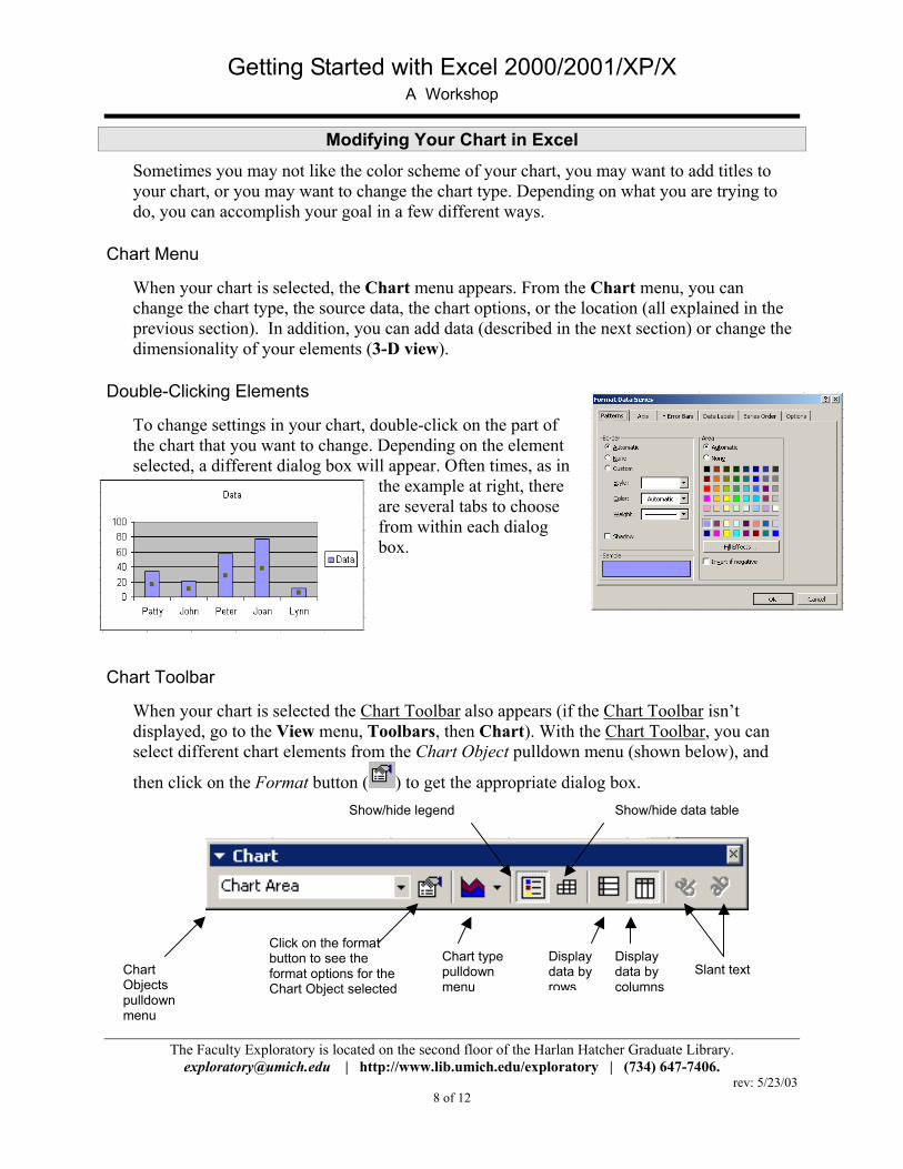
Double-Clicking Elements

To change settings in your chart, double-click on the part of the chart that you want to change. Depending on the element selected, a different dialog box will appear. Often times, as in

the example at right, there are several tabs to choose from within each dialog box.

Chart Toolbar

When your chart is selected the Chart Toolbar also appears (if the Chart Toolbar isn’t displayed, go to the View menu, Toolbars, then Chart). With the Chart Toolbar, you can select different chart elements from the Chart Object pulldown menu (shown below), and

then click on the Format button ( ) to get the appropriate dialog box.

Show/hide legend Show/hide data table

Chart type pulldown menu

Display data by rows

Display data by columns

Click on the format button to see the format options for the Chart Object selected

Chart Objects pulldown menu

Slant text


rev: 5/23/03 8 of 12


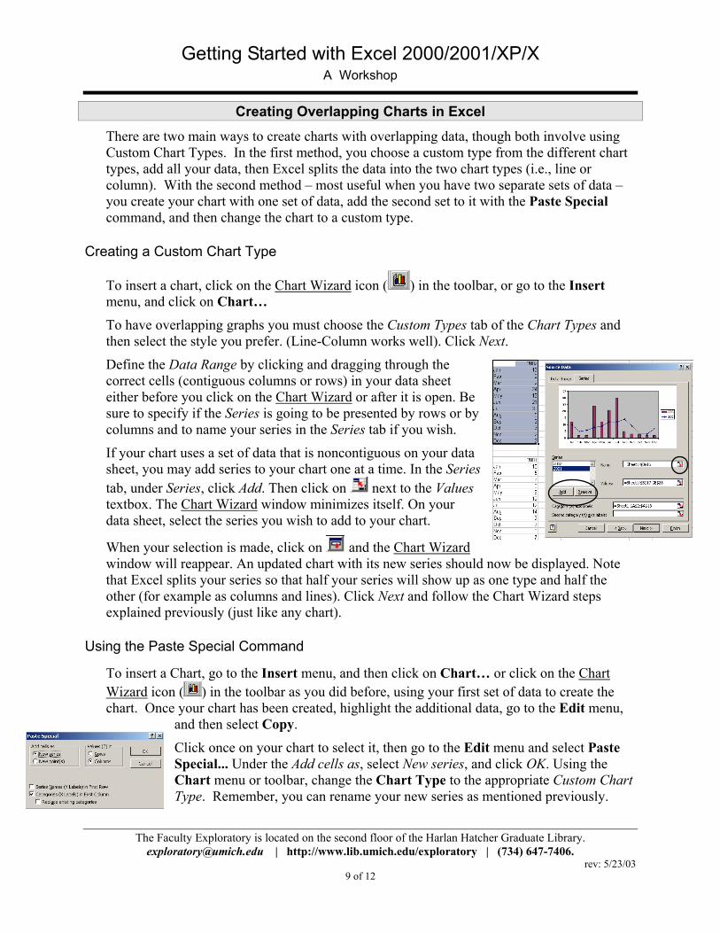
Creating Overlapping Charts in Excel There are two main ways to create charts with overlapping data, though both involve using Custom Chart Types. In the first method, you choose a custom type from the different chart types, add all your data, then Excel splits the data into the two chart types (i.e., line or column). With the second method – most useful when you have two separate sets of data – you create your chart with one set of data, add the second set to it with the Paste Special command, and then change the chart to a custom type.

Creating a Custom Chart Type

To insert a chart, click on the Chart Wizard icon ( ) in the toolbar, or go to the Insert menu, and click on Chart…

To have overlapping graphs you must choose the Custom Types tab of the Chart Types and then select the style you prefer. (Line-Column works well). Click Next.

Define the Data Range by clicking and dragging through the correct cells (contiguous columns or rows) in your data sheet either before you click on the Chart Wizard or after it is open. Be sure to specify if the Series is going to be presented by rows or by columns and to name your series in the Series tab if you wish.

If your chart uses a set of data that is noncontiguous on your data sheet, you may add series to your chart one at a time. In the Seriestab, under Series, click Add. Then click on

next to the Values

textbox. The Chart Wizard window minimizes itself. On your data sheet, select the series you wish to add to your chart.

When your selection is made, click on and the Chart Wizard window will reappear. An updated chart with its new series should now be displayed. Note that Excel splits your series so that half your series will show up as one type and half the other (for example as columns and lines). Click Next and follow the Chart Wizard steps explained previously (just like any chart).

Using the Paste Special Command

To insert a Chart, go to the Insert menu, and then click on Chart… or click on the Chart Wizard icon ( ) in the toolbar as you did before, using your first set of data to create the chart. Once your chart has been created, highlight the additional data, go to the Edit menu,

and then select Copy.

Click once on your chart to select it, then go to the Edit menu and select Paste Special... Under the Add cells as, select New series, and click OK. Using the Chart menu or toolbar, change the Chart Type to the appropriate Custom Chart Type. Remember, you can rename your new series as mentioned previously.


rev: 5/23/03 9 of 12


Formatting

Formatting Cells

Your spreadsheet cells may have several different formats. You can format the font, number, alignment, border, pattern, and protection by clicking selecting one or more cell and going to the Format menu, and then Cells… A window with a different tab for each type of format will appear. The different format options are:

• Number: Changes the format of the number. For example if the data in column A to should be currency, select the column, click on the Format menu, then Cells… Choose the Number tab, then select the Currency category.

• Alignment: Changes the alignment and orientation of the text. You can also choose to wrap text in a cell in this tab, or merge cells.

• Font: Changes the type of the font, its size and color.

• Border: Inserts borders around the select cell(s).

• Patterns: Changes the background color of the selected cell(s).

• Protection: Locks the cell(s)’ formula or hide it.

Formatting the Page

To add Headers and/or Footers, to change the margins or the page orientation or to print/not print gridlines, go to the File menu, select Page Setup, and then choose the appropriate tab.

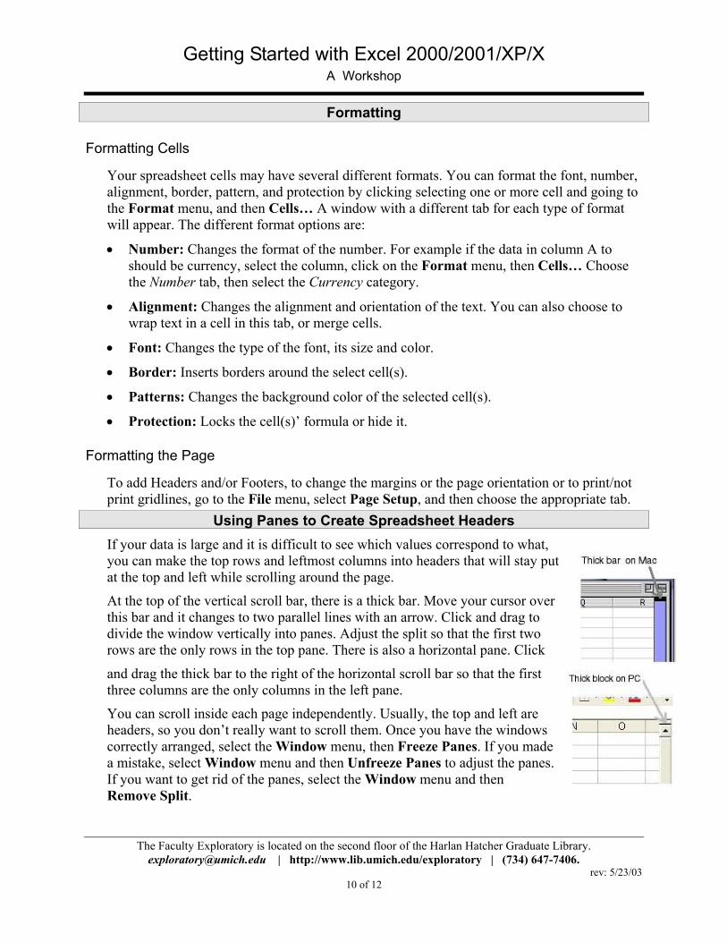
Using Panes to Create Spreadsheet Headers If your data is large and it is difficult to see which values correspond to what, you can make the top rows and leftmost columns into headers that will stay put at the top and left while scrolling around the page.

At the top of the vertical scroll bar, there is a thick bar. Move your cursor over this bar and it changes to two parallel lines with an arrow. Click and drag to divide the window vertically into panes. Adjust the split so that the first two rows are the only rows in the top pane. There is also a horizontal pane. Click

and drag the thick bar to the right of the horizontal scroll bar so that the first three columns are the only columns in the left pane.

You can scroll inside each page independently. Usually, the top and left are headers, so you don’t really want to scroll them. Once you have the windows correctly arranged, select the Window menu, then Freeze Panes. If you made a mistake, select Window menu and then Unfreeze Panes to adjust the panes. If you want to get rid of the panes, select the Window menu and then Remove Split.


rev: 5/23/03 10 of 12


Weighted Averages Suppose the final exam is 50% of the grade, and the homework and midterm are 25% each. To make a weighted average, each score is multiplied by the decimal equivalent of its weight, and the weighted scores are added up. The only restriction on a weighted average is that the weights must sum to 1 (or 100%). (Note for advanced users: The weighted sum formula can be entered by hand (e.g. ‘=0.25*q3+0.25*r3+0.5*s3’ for the first student).

Quick Reference: 1. Enter weights 2. Select and Name weights 3. Paste sumproduct function (see #4

below) a. Array 1 = first student's scores b. Array 2 = Weights

4. Click OK and autofill

We could enter those weights at the bottom of each column and then use Excel's function called sumproduct. However, if we use the fill command for the rest of the students, the cell references for the weights would also move. By defining a named area with the weights in it, we can reference those cells with a specific name and lock them in relationship to the students' scores.

Before we start, create a new column for the weighted averages for all of the students. This way we can compare the weighted averages with the non-weighted averages.

Defining a Named Area

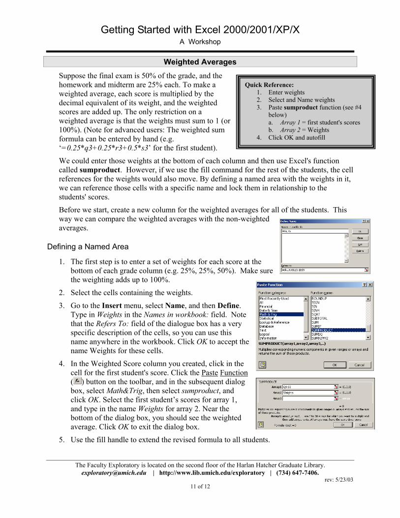
1. The first step is to enter a set of weights for each score at the bottom of each grade column (e.g. 25%, 25%, 50%). Make sure the weighting adds up to 100%.

2. Select the cells containing the weights.

3. Go to the Insert menu, select Name, and then Define. Type in Weights in the Names in workbook: field. Note that the Refers To: field of the dialogue box has a very specific description of the cells, so you can use this name anywhere in the workbook. Click OK to accept the name Weights for these cells.

4. In the Weighted Score column you created, click in the cell for the first student's score. Click the Paste Function ( ) button on the toolbar, and in the subsequent dialog box, select Math&Trig, then select sumproduct, and click OK. Select the first student’s scores for array 1, and type in the name Weights for array 2. Near the bottom of the dialog box, you should see the weighted average. Click OK to exit the dialog box.

5. Use the fill handle to extend the revised formula to all students.


rev: 5/23/03 11 of 12



rev: 5/23/03 12 of 12

Substituting Letter Grades Substituting Letter Grades Quick Reference:

5. Create Columns 6. Add Scale and Letter Grades 7. Select Scale and Letters and name

them (#6 below) 8. Paste vlookup function (see #7-10)

a. Look_up value = first students score e

b. Table_array = Scale b. Table_array = Scale c. Col_index_num = 2 c. Col_index_num = 2

9. Click OK and auto-fill formula 9. Click OK and auto-fill formula

Rather than entering letter grades by hand, Excel can do it for you. This also allows you to try different grading curves with a minimum of effort.

Rather than entering letter grades by hand, Excel can do it for you. This also allows you to try different grading curves with a minimum of effort. 1. Create column a column for the students called

Grade. 1. Create column a column for the students called

Grade. 2. Add two other headings for Scale and Letter

Grade. Under Scale, enter a straight scale by typing 0, 60, 70, 80, 90, down the column. For automatic grade assignment, you must start with the low score and increase as you go down.

2. Add two other headings for Scale and Letter Grade. Under Scale, enter a straight scale by typing 0, 60, 70, 80, 90, down the column. For automatic grade assignment, you must start with the low score and increase as you go down.

3. Under Letter Grade, enter ‘E’, ‘D’, ‘C’, ‘B’, ‘A’. 3. Under Letter Grade, enter ‘E’, ‘D’, ‘C’, ‘B’, ‘A’. 4. We want to use the same curve for all students (remember references are usually relative,

and will change when a formula is copied). Just like with the weights, we will refer to this curve by giving it a name so we won’t have to worry about the cell reference.

4. We want to use the same curve for all students (remember references are usually relative, and will change when a formula is copied). Just like with the weights, we will refer to this curve by giving it a name so we won’t have to worry about the cell reference.

5. Select the scale scores and the letter grades (but not the headings). 5. Select the scale scores and the letter grades (but not the headings). 6. Go to the Insert menu, then Name, and then Define. Type in the name ‘Scale’ as a

reference to the cells we selected. Click OK to accept the name. Now we’re ready to use that scale to assign grades.

6. Go to the Insert menu, then Name, and then Define. Type in the name ‘Scale’ as a reference to the cells we selected. Click OK to accept the name. Now we’re ready to use that scale to assign grades.

7. Go to the Grade column for the first student. Click on the Paste Function7. Go to the Grade column for the first student. Click on the Paste Function ( ) button. Select Lookup & Reference and then Vlookup (short for vertical table lookup). Click OK. 8. The vlookup function looks up a value in the first column of a table

(where the values in the first column are increasing) and returns the value in any column of the table. Click once in the lookup_value field; this is the

cumulative score we want to compare to the curve. Click on the Cum Score of the first student and it will now display that value in the lookup_value field.

9. Click in the table_array field. Type in ‘Scale’, which is the name of our table of grades. 10. Click in the col_index_num field; this is the column of the table that we want the lookup function to return. We want the letter grade, which is in the 2nd column, so put 2 in this field. 11. Note the range_lookup argument is not bold. That means it’s optional. 12. Click OK, and note whether the correct grade has been entered. 13. Use the fill handle to fill the formula in to the rest of the students. Note that we don’t have to worry about the reference to our scale because we used a name. You can change the curve to something else (e.g. 55, 65, 75, 85) and see how that influences the grades.

Documents

Getting Started with Excel 2000/2001/XP/Xexphysio/mvs110l/excel2000_XP.pdf · Getting Started with Excel 2000/2001/XP/X A Workshop Overview Excel is an excellent tool for data storage