Embed Size (px)
DESCRIPTION
Chemistry versus PhysicsChemical reactions near critical pointsAuthor: M. GittermanIn this book we attempt to trace the connection between chemical reactions and the physical forces of interaction manifested in critical phenomena.
Citation preview


Chemical Reactions Near Critical PointsPHYSICS
CHEMISTRYVERSUS

This page intentionally left blankThis page intentionally left blank

Chemical Reactions Near Critical PointsPHYSICS
CHEMISTRYVERSUS
N E W J E R S E Y • L O N D O N • S I N G A P O R E • B E I J I N G • S H A N G H A I • H O N G K O N G • TA I P E I • C H E N N A I
World Scientific
Moshe GittermanBar-Ilan University, Israel
British Library Cataloguing-in-Publication DataA catalogue record for this book is available from the British Library.
For photocopying of material in this volume, please pay a copying fee through the CopyrightClearance Center, Inc., 222 Rosewood Drive, Danvers, MA 01923, USA. In this case permission tophotocopy is not required from the publisher.
ISBN-13 978-981-4291-20-0ISBN-10 981-4291-20-X
All rights reserved. This book, or parts thereof, may not be reproduced in any form or by any means,electronic or mechanical, including photocopying, recording or any information storage and retrievalsystem now known or to be invented, without written permission from the Publisher.
Copyright © 2010 by World Scientific Publishing Co. Pte. Ltd.
Published by
World Scientific Publishing Co. Pte. Ltd.
5 Toh Tuck Link, Singapore 596224
USA office: 27 Warren Street, Suite 401-402, Hackensack, NJ 07601
UK office: 57 Shelton Street, Covent Garden, London WC2H 9HE
Printed in Singapore.
CHEMISTRY VERSUS PHYSICSChemical Reactions Near Critical Points
ZhangFang - Chemistry vs Physics.pmd 9/10/2009, 7:09 PM1
September 14, 2009 16:24 World Scientific Book - 9in x 6in General-nn
Preface
In this book we attempt to trace the connection between chemical reactions
and the physical forces of interaction manifested in critical phenomena.
The physical and chemical descriptions of matter are intimately related. In
fact, the division of forces into “physical” and “chemical” is arbitrary. It
is convenient [1] to distinguish between strong attractive (chemical) forces
leading to the formation of chemical species, and weak attractive (physical)
forces, called van der Waals forces. It should be remembered, therefore,
when one considers the “ideal” ternary mixture A, B and AmBn, that the
strong chemical bonding interaction between A and B atoms has already
been taken into account via the formation of the chemical complex AmBn,
and the term “ideal” only means that there are no “physical” forces present.
The growth of clusters in a metastable state is an example of the fuzzy
distinction between physical and chemical forces. In numerical simulations
a rather arbitrary decision has to be made whether a given particle belongs
to a “chemical” cluster.
The usefulness of a “chemical” approach to physical problems can be
seen from the mean-field theory of the phase transition on an Ising lattice
of non-stoichiometric AB alloys [2]. The temperature dependence of the
long-range and short-range order parameters is found from the “law of mass
action” for the appropriately chosen “chemical reaction.” The latter is the
exchange of position of an atom A from one sublattice and an atom B
from the second sublattice. The change of the interaction energy for such a
transition when both atoms are or are not nearest neighbors determines the
“constant of chemical reaction.” Such an approach allows one to avoid the
calculation of entropy provided that one is interested only in the value of
the critical temperature, rather than in the behavior of all thermodynamic
quantities, which are determined by the same classical critical indices in
v
September 14, 2009 16:24 World Scientific Book - 9in x 6in General-nn
vi Chemistry versus Physics: Chemical Reactions near Critical Points
all versions of mean-field theory. The latter example is, in fact, a special
case of chapter 15 in [3], where the typical “physical” process of diffusion
is considered as a “chemical reaction” in which some amount of substance
A passes from volume element a to b while a different amount of B passes
from b to a.
The “chemical” method, in which a given atom with all its neighbors is
considered as the basic group, gives better results than the Bragg-Williams
or Bethe-Peierls method. In the Bragg-Williams method, each atom is
exposed to the (self-consistent) average influence of all other atoms, whereas
in the Bethe-Peierls method, a pair of adjacent atoms is considered as the
basic group.
Even though the border between chemical and physical forces is arbi-
trary, one usually considers first the “physical” forces in the equation of
state, and then the “chemical” forces in the law of mass action based on
the non-ideal equation of state. I shall follow this approach.
One can also trace the common features of phase transitions and chem-
ical reactions by analyzing the time evolution of the state variables ψ de-
scribed by the equation
dψ/dt = F [ψ, λ] , (0.1)
where λ is the set of internal and external parameters, and F is a nonlinear
functional in ψ. In the case of a phase transition, Eq. (0.1) may be the
Landau-Ginzburg equation for the order parameter, while in the case of
a chemical reaction — the equation for the rate of reaction. The steady
state of the system is described by ψ0 (λ) which is the solution of equation
F[ψ0, λ
]= 0. For nonlinear F , more than one steady state solution is pos-
sible, and for some values of λ, at the so-called transition point, bifurcation
may occur, when a system goes from the original steady state to the new
steady state. Such a transition might be of first or second order in the case
of a phase transition, and, analogously, the hard or soft transition for a
chemical reaction.
I have kept this book as simple as possible, so that it will be useful
for a wide range of researchers, both physicists and chemists, as well as
teachers and students. No preliminary knowledge is assumed, other than
undergraduate courses in general physics and chemistry. In line with this
approach, I have favored a phenomenological presentation, thus avoiding
the details of both microscopic and numerical approaches. There are a
tremendous number of published articles devoted to this subject, and it
proved impossible to include many of them in this book of small size. I ask

September 14, 2009 16:24 World Scientific Book - 9in x 6in General-nn
Preface vii
the forgiveness of the authors whose publications were beyond the scope of
this book.
The organization of the book is as follows.
After the Introduction, Chapter 1 contains a short review of phase tran-
sitions and chemical reactions and their interconnection, which is needed
to understand the ensuing material. Chapter 2 is devoted to the specific
changes in a chemical reaction occurring near the critical point. The effect
of pressure and phase transformation on the equilibrium constant and rate
of reaction is the subject of Secs. 2.1–2.2. The hallmark of critical phenom-
ena — the slowing down of all processes — leads also to the slowing-down of
the rates of chemical reactions. This phenomenon is described in Sec. 2.3,
while the opposite peculiar phenomenon of speeding-up of a chemical re-
action near the critical point provides the subject matter for Sec. 2.4. It
is shown that all three types of behavior (slowing-down, speeding-up and
unchanged) are possible depending on the given experiment. In Sec. 2.5,
we consider another influence of criticality — the anomalies in chemical
equilibria including supercritical extraction. The appropriate experiments
are described in Sec. 2.6.
The reverse process — influence of chemistry on critical phenomena —
forms the content of Chapter 3, including the change in the critical param-
eters (Sec. 3.1), critical indices (Sec. 3.2), transport coefficients (Sec. 3.5)
and degree of dissociation (Sec. 3.3). Section 3.4 is devoted to the isotope
exchange reaction in near-critical systems.
Chapter 4 deals with the problem of the phase separation in reactive
systems. The occurrence of multiple solutions of the law of mass action
is described in Sec. 4.1. The mechanism of phase separation depends on
whether it starts from a metastable or a non-stable state. The former case,
where phase separation takes place through nucleation, and the spinodal
decomposition for the latter case are considered in Secs. 4.2 and 4.3, respec-
tively. Section 4.4 is devoted to the special case of a dissociation reaction
in a ternary mixture.
Chapter 5 contains a description of chemical reactions near some specific
regions of the phase diagram. An account of the supercritical fluids is given
in Sec. 5.1, while the vicinities of the azeotrope, melting and double critical
points are considered in Secs. 5.2, 5.3 and 5.4, respectively. The main ex-
perimental methods of analysis of near-critical fluids — sound propagation
and light scattering — are considered in Chapter 6. Finally, in Chapter 7
we present our conclusions.
September 14, 2009 16:24 World Scientific Book - 9in x 6in General-nn
Contents
Preface v
1. Criticality and Chemistry 1
1.1 Critical phenomena . . . . . . . . . . . . . . . . . . . . . . 1
1.2 Chemical reactions . . . . . . . . . . . . . . . . . . . . . . 8
1.3 Analogy between critical phenomena and the instability of
chemical reactions . . . . . . . . . . . . . . . . . . . . . . 12
2. Effect of Criticality on Chemical Reaction 15
2.1 The effect of pressure on the equilibrium constant and rate
of reaction . . . . . . . . . . . . . . . . . . . . . . . . . . . 15
2.2 Effect of phase transformations on chemistry . . . . . . . 17
2.3 Critical slowing-down of chemical reactions . . . . . . . . 19
2.4 Hydrodynamic equations of reactive binary mixture:
piston effect . . . . . . . . . . . . . . . . . . . . . . . . . . 25
2.4.1 Heterogeneous reactions in near-critical systems . 26
2.4.2 Dynamics of chemical reactions . . . . . . . . . . 27
2.4.3 Relaxation time of reactions . . . . . . . . . . . . 29
2.4.4 Hydrodynamic equations of a reactive binary
mixtures . . . . . . . . . . . . . . . . . . . . . . . 32
2.4.5 Hydrodynamic equations with statistically
independent variables . . . . . . . . . . . . . . . 38
2.5 Critical anomalies of chemical equilibria . . . . . . . . . . 46
2.6 Experiment . . . . . . . . . . . . . . . . . . . . . . . . . . 48
3. Effect of Chemistry on Critical Phenomena 53
ix
September 14, 2009 16:24 World Scientific Book - 9in x 6in General-nn
x Chemistry versus Physics: Chemical Reactions near Critical Points
3.1 Change of critical parameters due to a chemical reaction . 53
3.2 Modification of the critical indices . . . . . . . . . . . . . 55
3.3 Singularity in the degree of dissociation near a critical point 60
3.4 Isotope exchange reaction in near-critical systems . . . . . 62
3.5 Singularities of transport coefficients in reactive systems . 63
3.5.1 Mode-coupling analysis . . . . . . . . . . . . . . . 63
3.5.2 Renormalization group methods . . . . . . . . . . 65
4. Phase Separation in Reactive Systems 67
4.1 Multiple solutions of the law of mass action . . . . . . . . 67
4.2 Phase equilibrium in reactive binary mixtures quenched
into a metastable state . . . . . . . . . . . . . . . . . . . . 69
4.2.1 Thermodynamic analysis of reactive binary
mixtures . . . . . . . . . . . . . . . . . . . . . . . 69
4.2.2 Thermodynamic analysis of reactive ternary
mixtures . . . . . . . . . . . . . . . . . . . . . . . 72
4.2.3 Kinetics of phase separation . . . . . . . . . . . . 75
4.3 Phase equilibrium in reactive mixtures quenched into an
unstable state . . . . . . . . . . . . . . . . . . . . . . . . . 81
4.4 Thermodynamics of a three-component plasma with a
dissociative chemical reaction . . . . . . . . . . . . . . . . 89
5. Comments on the Geometry of the Phase Diagram of a
Reaction Mixture 93
5.1 Solubility in supercritical fluids . . . . . . . . . . . . . . . 93
5.2 Azeotropic points in reactive many-component systems . . 100
5.3 Melting point of reactive binary mixtures . . . . . . . . . 101
5.4 Double critical point . . . . . . . . . . . . . . . . . . . . . 105
6. Sound Propagation and Light Scattering in Chemically
Reactive Systems 111
6.1 Ultrasound attenuation in near-critical reactive mixtures . 111
6.2 Hydrodynamic analysis of the dispersion relation for sound
waves . . . . . . . . . . . . . . . . . . . . . . . . . . . . . 113
6.3 Light scattering from reactive systems . . . . . . . . . . . 118
6.4 Inhomogeneous structure of near-critical reactive systems 121
7. Conclusions 125

September 14, 2009 16:24 World Scientific Book - 9in x 6in General-nn
Contents xi
Bibliography 127
Index 135
September 11, 2009 10:7 World Scientific Book - 9in x 6in General-nn
Chapter 1
Criticality and Chemistry
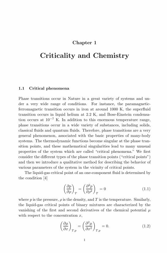
1.1 Critical phenomena
Phase transitions occur in Nature in a great variety of systems and un-der a very wide range of conditions. For instance, the paramagnetic-ferromagnetic transition occurs in iron at around 1000 K, the superfluidtransition occurs in liquid helium at 2.2 K, and Bose-Einstein condensa-tion occurs at 10−7 K. In addition to this enormous temperature range,phase transitions occur in a wide variety of substances, including solids,classical fluids and quantum fluids. Therefore, phase transitions are a verygeneral phenomenon, associated with the basic properties of many-bodysystems. The thermodynamic functions become singular at the phase tran-sition points, and these mathematical singularities lead to many unusualproperties of the system which are called “critical phenomena.” We firstconsider the different types of the phase transition points (“critical points”)and then we introduce a qualitative method for describing the behavior ofvarious parameters of the system in the vicinity of critical points.
The liquid-gas critical point of an one-component fluid is determined bythe condition [4] (
∂p
∂ρ
)T
=(∂2p
∂ρ2
)T
= 0 (1.1)
where p is the pressure, ρ is the density, and T is the temperature. Similarly,the liquid-gas critical points of binary mixtures are characterized by thevanishing of the first and second derivatives of the chemical potential µwith respect to the concentration x,(
∂µ
∂x
)T,p
=(∂2µ
∂x2
)T,p
= 0. (1.2)
1
September 11, 2009 10:7 World Scientific Book - 9in x 6in General-nn
2 Chemistry versus Physics: Chemical Reactions near Critical Points
Here µ = µ1/m1 − µ2/m2, where µ1, µ2 and m1, m2 are the chemicalpotentials and masses of the two components.
The close relation between (1.1) and (1.2) is evident from the equivalentform of Eq. (1.2), which can be rewritten as(
∂p
∂ρ
)T,µ
=(∂2p
∂ρ2
)T,µ
= 0. (1.3)
The critical conditions for a binary mixture (1.3) are the same as thosefor a pure system (1.1) when the chemical potential is kept constant. Anal-ogously, the critical points for an n-component mixture are determined bythe conditions (
∂p
∂ρ
)T,µ1,...,µn−1
=(∂2p
∂ρ2
)T,µ1,...,µn−1
= 0 (1.4)
where n− 1 chemical potentials are held constant.In addition to the above-mentioned thermodynamic peculiarities, relax-
ation processes slow down near the critical points resulting in singularitiesin the kinetic coefficients. An example is the slowing-down of diffusion nearthe critical points of a binary mixture. Nothing happens to the motion ofthe separate molecules when one approaches the critical point. It is the rateof equalization of the concentration gradients by diffusion which is reducednear the critical points. In fact, the excess concentration δx in some partof a system does not produce diffusion by itself. Usually a system has nodifficulty in “translating” the change in concentration into a change in thechemical potential δµ ∼ (∂µ/∂x) δx, which is the driving force for diffusion.However, near the critical point, according to (1.2), ∂µ/∂x is very small,and the system becomes indifferent to changes in concentration. This isthe simple physical explanation of the slowing-down of diffusion near thecritical point.
Since the states of a one-component system and a binary mixture are de-fined by the equations of state p = p (T, µ) and µ = µ (T, ρ, x) , respectively,Eqs. (1.1) and (1.2) define the isolated critical point for an one-componentsystem, and the line of critical points for a binary mixture. Another dis-tinction between one-component systems and binary mixtures is that thereare two types of critical points in the latter: the above considered liquid-gascritical points and liquid-liquid critical points, whereas two coexisting liq-uid phases are distinguished by different concentrations of the components.Both critical lines are defined by Eq. (1.2).
Different binary liquid mixtures show either concave-down or concave-up coexistence curves in a temperature-concentration phase diagram (at
September 11, 2009 10:7 World Scientific Book - 9in x 6in General-nn
Criticality and Chemistry 3
fixed pressure) or in a pressure-concentration phase diagram (at fixed tem-perature). The consolute point is an extremum in the phase diagram wherethe homogeneous liquid mixture first begins to separate into two immiscibleliquid layers. For the concave-down diagram, as for a methanol-heplan mix-ture, the minimum temperature above which the two liquids are misciblein all proportions is called the upper critical solution temperature (UCST).By contrast, for a concave-up diagram, such as the water-triethylamine so-lution, the maximum temperature below which the liquids are miscible inall proportions is called the lower critical solution temperature (LCST).Under the assumption of analyticity of the thermodynamic functions atthe critical points, one can obtain the general thermodynamic criterionfor the existence of UCST and LCST [3]. We will discuss this calculationin the next section when examinating the influence of chemical reactionson UCST and LCST. Here we will consider chemical reactions occurringbetween solutes near the critical points of the solvent.
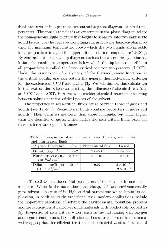
The properties of near-critical fluids range between those of gases andliquids (see Table 1). Near-critical fluids combine properties of gases andliquids. Their densities are lower than those of liquids, but much higherthan the densities of gases, which makes the near-critical fluids excellentsolvents for a variety of substances.
Table 1. Comparison of some physical properties of gases, liquidsand near-critical fluids.
Physical Properties Gas Near-critical fluid Liquid
Density (kg/m3) 0.6–2 200–500 600–1000
Kinematic viscosity 5–500 0.02–0.1 0.1–5(10−6m2/sec)
Diffusion coefficient 10–40 0.07 2 × 10⁻⁴–(10−6 m2/ sec) 2 × 10⁻³
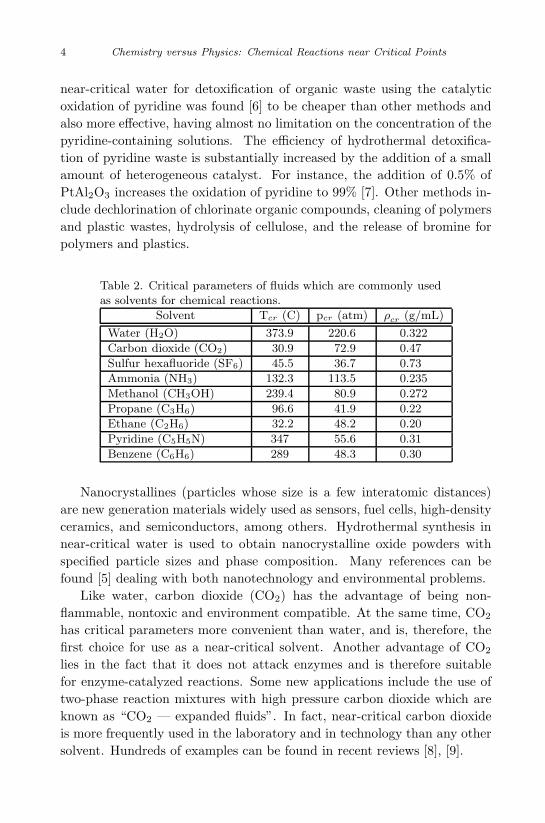
In Table 2 we list the critical parameters of the solvents in most com-mon use. Water is the most abundant, cheap, safe and environmentallypure solvent. In spite of its high critical parameters which limits its ap-plication, in addition to the traditional uses, modern applications includethe important problems of solving the environmental pollution problemand the fabrication of nanocrystalline materials with predictable properties[5]. Properties of near-critical water, such as the full mixing with oxygenand organic compounds, high diffusion and mass transfer coefficients, makewater appropriate for efficient treatment of industrial wastes. The use of
September 11, 2009 10:7 World Scientific Book - 9in x 6in General-nn
4 Chemistry versus Physics: Chemical Reactions near Critical Points
near-critical water for detoxification of organic waste using the catalyticoxidation of pyridine was found [6] to be cheaper than other methods andalso more effective, having almost no limitation on the concentration of thepyridine-containing solutions. The efficiency of hydrothermal detoxifica-tion of pyridine waste is substantially increased by the addition of a smallamount of heterogeneous catalyst. For instance, the addition of 0.5% ofPtAl2O3 increases the oxidation of pyridine to 99% [7]. Other methods in-clude dechlorination of chlorinate organic compounds, cleaning of polymersand plastic wastes, hydrolysis of cellulose, and the release of bromine forpolymers and plastics.
Table 2. Critical parameters of fluids which are commonly usedas solvents for chemical reactions.
Solvent Tcr (C) pcr (atm) ρcr (g/mL)
Water (H2O) 373.9 220.6 0.322
Carbon dioxide (CO2) 30.9 72.9 0.47
Sulfur hexafluoride (SF6) 45.5 36.7 0.73
Ammonia (NH3) 132.3 113.5 0.235
Methanol (CH3OH) 239.4 80.9 0.272
Propane (C3H6) 96.6 41.9 0.22
Ethane (C2H6) 32.2 48.2 0.20
Pyridine (C5H5N) 347 55.6 0.31
Benzene (C6H6) 289 48.3 0.30
Nanocrystallines (particles whose size is a few interatomic distances)are new generation materials widely used as sensors, fuel cells, high-densityceramics, and semiconductors, among others. Hydrothermal synthesis innear-critical water is used to obtain nanocrystalline oxide powders withspecified particle sizes and phase composition. Many references can befound [5] dealing with both nanotechnology and environmental problems.
Like water, carbon dioxide (CO2) has the advantage of being non-flammable, nontoxic and environment compatible. At the same time, CO2
has critical parameters more convenient than water, and is, therefore, thefirst choice for use as a near-critical solvent. Another advantage of CO2
lies in the fact that it does not attack enzymes and is therefore suitablefor enzyme-catalyzed reactions. Some new applications include the use oftwo-phase reaction mixtures with high pressure carbon dioxide which areknown as “CO2 — expanded fluids”. In fact, near-critical carbon dioxideis more frequently used in the laboratory and in technology than any othersolvent. Hundreds of examples can be found in recent reviews [8], [9].
September 11, 2009 10:7 World Scientific Book - 9in x 6in General-nn
Criticality and Chemistry 5
The infinite increase of the compressibility ρ−1 (∂ρ/∂p)T or (∂x/∂µ)T,p
as the critical point is approached, leads to a number of peculiarities in thebehavior of a substance near its critical point. The specific heat at constantpressure Cp and the expansion coefficient β = −ρ−1 (∂ρ/∂T )p also increasenear the critical point of a one-component system, as follows from Eq. (1.1)and the appropriate thermodynamic relations.
A sharp increase in the mean square fluctuations of the density (orconcentration) and of the integral of the correlation function gρρ followsfrom the well-known thermodynamic relations
(ρ (r) − ρ)2 ∼(∂ρ
∂p
)T
→∞;∫gρρd
3r ∼(∂ρ
∂p
)T
→∞. (1.5)
The large increase of the correlations between the positions of differentparticles is given by the second expression in (1.5), which is closely con-nected with the first expression. In other words, widely separated particleshave to be strongly correlated to cause great changes in density.
The correlation radius ξ, which characterizes the distance over whichcorrelations are significant, increases sharply near the critical temperatureTC ,
ξT→TC→∞. (1.6)
According to estimates from scattering experiments, ξ reaches 10−4− 10−5
cm near the critical point. Thus, the specific nature of the critical regionconsists of the appearance of a new characteristic distance ξ, satisfying thecondition
a << ξ << R (1.7)
where a is the average distance between particles and R is a characteristicmacroscopic length.
As an illustration of the crucial importance of the new characteristiclength ξ, let us consider the singular part of the transport coefficients nearthe critical point for a model fluid consisting of spheres with a characteristicradius ξ. Particles inside such spheres are strongly correlated, and we canassume that under the influence of an external force, they move togetherwith a mean velocity v and a mean free path ξ. One finds the followingresults [10]:
1. Diffusion coefficient [11]. When an external force F is applied, thespheres move according to Stoke’s law, F ∼ ηξv, where η is the viscosity,i.e., the mobility b ≡ v/F ∼ (ηξ)−1. Using the Einstein relationD = kBTb,
September 11, 2009 10:7 World Scientific Book - 9in x 6in General-nn
6 Chemistry versus Physics: Chemical Reactions near Critical Points
where D is the diffusion coefficient and kB is the Boltzmann constant, wehave D ∼ (ηξ)−1 or Dη ∼ ξ−1, a result confirmed by the more rigoroustheory and by experiment.
2. Heat conductivity. The usual arguments of molecular-kinetictheory give the heat flux q passing through unit area per unit time,q ∼ υn (ε1 − ε2) . Here, n is the total number of spheres, and ε1 − ε2 isthe difference in their energies on two sides of a selected area, arising fromthe temperature difference T1−T2 ∼ ξ∇T : ε1− ε2 ∼ V Cpξ∇T , where V isthe total volume of the spheres, so that nV = 1. Thus, q ∼ vCpξ∇T.One can find the velocity v from the estimate for the diffusion coeffi-cient given above: v ∼ D/ξ ∼ 1/ξ2η. Finally, the heat conductivityλ ∼ q/∇T ∼ vCpξ ∼ Cp/ηξ. This result is supported by more rigoroustheory and also by experiment.
The qualitative description of the singularity of the quantity a atthe critical point is given by the non-integer critical index x, wherea ∼ |T−TC |x. If x �= 0, this critical index is given by x = ln(a)/ ln |T −TC |,whereas if x = 0, there are two possibilities. In one case, a becomes constantat the critical point, with the possibility of different values of this constanton the two sides of the transition, which is called a jump singularity. In theother case, a exhibits a logarithmic singularity, a ∼ ln |T − TC |.
Although there are general properties which define the values of the crit-ical indices (dimension d of space, symmetry and the presence of long-rangeinteractions), according to the universality principle, these values are de-fined by the general statistical properties of the many-body system, ratherthan by the details of the microscopic interactions. This implies that dif-ferent isomorphic systems will have the same indices for the appropriateparameters. Using the language of fluids, the commonly accepted sym-bols α, β, γ, δ, η, and ν describe, respectively, the asymptotic behavior nearthe one-component liquid-gas critical point of the specific heat at constantvolume, order parameter (deviation of the density from its critical value),compressibility, pressure-density relation at the critical isotherm, the cor-relation function at the critical temperature, and the correlation length.Of these indices, one (β) is determined only below the critical temperatureand two (δ, η) exist only at the critical temperature. The remaining threeindices can be defined for temperatures above critical (α, γ, ν) as well asbelow (α′, γ′, ν′). According to scaling theory [12], α = α′, γ = γ′, ν = ν ′
and the following relations exist between critical indices: α + 2β + γ = 2,dν = 2− α, (2− η) ν = γ, and β (δ − 1) = γ.
September 11, 2009 10:7 World Scientific Book - 9in x 6in General-nn
Criticality and Chemistry 7
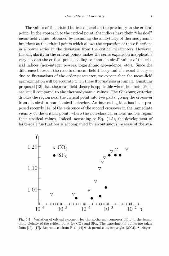
The values of the critical indices depend on the proximity to the criticalpoint. In the approach to the critical point, the indices have their “classical”mean-field values, obtained by assuming the analyticity of thermodynamicfunctions at the critical points which allows the expansion of these functionsin a power series in the deviation from the critical parameters. However,the singularity in the critical points makes the series expansion inapplicablevery close to the critical point, leading to “non-classical” values of the crit-ical indices (non-integer powers, logarithmic dependence, etc.). Since thedifference between the results of mean-field theory and the exact theory isdue to fluctuations of the order parameter, we expect that the mean-fieldapproximation will be accurate when these fluctuations are small. Ginzburgproposed [13] that the mean field theory is applicable when the fluctuationsare small compared to the thermodynamic values. The Ginzburg criteriondivides the region near the critical point into two parts, giving the crossoverfrom classical to non-classical behavior. An interesting idea has been pro-posed recently [14] of the existence of the second crossover in the immediatevicinity of the critical point, where the non-classical critical indices regaintheir classical values. Indeed, according to Eq. (1.5), the development oflarge-scale fluctuations is accompanied by a continuous increase of the sus-
Fig. 1.1 Variation of critical exponent for the isothermal compressibility in the imme-diate vicinity of the critical point for CO2 and SF6. The experimental points are takenfrom [16], [17]. Reproduced from Ref. [14] with permission, copyright (2002), Springer.

September 11, 2009 10:7 World Scientific Book - 9in x 6in General-nn
8 Chemistry versus Physics: Chemical Reactions near Critical Points
ceptibilities of the critical system, in particular, the susceptibility to variesexternal perturbations (gravitational and Coulomb fields, surface forces,shear stresses, turbulence, presence of boundaries). As a consequence, clas-sical mean-field behavior must be restored. This transition occurs in thedirection opposite to the Ginzburg criterion direction and defines the sec-ond crossover. Such behavior was found experimentally as early as 1974[15] by taking p− V − T measurements of very pure SF6 in the immediatevicinity (τ = T−TC
TC) of the critical point with 2 × 10⁻⁴K, ±0.01%, and
±0.02% accuracy, respectively in the temperature, dimensionless pressureand density.
As an example, we show [14] in Fig. 1.1 the crossover to the classicalvalue of the critical index of the isothermal compressibility in the immedi-ate vicinity of the critical point for CO2 and SF6. The author of [14] stateshis belief that the analogous second crossover has been seen in other ex-periments under the influence of gravity, impurities, and shear flows. Thisproblem certainly deserves further investigation.
1.2 Chemical reactions
The equilibrium numbers of particles of the different substances taking partin a chemical reaction are connected by the law of mass action. This lawresults from a relation between the chemical potentials µi of the variouscomponents [3]. Thus, for the reaction
∑νiAi = 0 , where Ai are the
chemical symbols of the reagents and νi are positive or negative integers,the equation for chemical equilibrium has the form
∑νiµi = 0. For the
simplest case of the isomerization reaction, the reaction equation and thelaw of mass action have the form A1 −A2 = 0 and µ1 = µ2, respectively.
Thus, binary mixtures undergoing a chemical reaction are characterizedby their concentration, as in a non-reactive mixture. However, accordingto the law of mass action, this concentration is a function of other ther-modynamic variables. Therefore, the number of thermodynamic degrees offreedom of a binary system undergoing a chemical reaction is the same asfor a non-reactive, one-component system.
Chemical reactions influence all properties of many-component systems.As an example, we shall show that the existence of the chemical reactionmay lead to the replacement of UCST by LCST and vice versa [18]. More-over, the Clapeyron-Clausius equation for a binary mixture is determinedby the chemical reaction, in addition to the latent heat and the volumedifference between the two phases.
September 11, 2009 10:7 World Scientific Book - 9in x 6in General-nn
Criticality and Chemistry 9
Consider a mole of a binary mixture which separates into two phases,B′ and B′′. The system can be described by four parameters, p, T, x′2, andx′′2 , which satisfy the following conditions:
µ′1 (T, p, x′2) = µ′′
1 (T, p, x′′2) ; µ′2 (T, p, x′2) = µ′′
2 (T, p, x′′2) . (1.8)
One can differentiate the equilibrium conditions (1.8) along the equilib-rium surface between B′ and B′′. Using simple thermodynamic relations,one obtains [3]
∆υ1dp−∆h1dT/T + x′2g′2xdx′2 − x′′2g′′2xdx
′′2 = 0,
∆υ2dp−∆h2dT/T + (1− x′′2 ) g′′2xdx′′2 −
(1− x�
2
)g′2xdx
′2 = 0 (1.9)
where υi and hi are the partial molar volume and enthalpy,
∆υi = υ′′i − υ′i; ∆hi = h′′i − h′i; g′2x ≡(∂2g′
∂x′22
)T,p
; g′′2x ≡(∂2g′′
∂x′′22
)T,p
.
(1.10)The partial derivatives of the intensive variables are given by Eq. (1.9)
at constant pressure (temperature) and at constant concentration [3]. How-ever, there is no need to consider these special sections of the coexis-tence surface when we deal with a reactive system. Indeed, for a reactionν1A1 � ν2A2, an additional restriction to (1.9) exists in the form of thelaw of mass action
ν1µ′1 + ν2µ
′2 = 0. (1.11)
Differentiating the latter equation along the equilibrium surface, yields
(ν1υ′1 + ν2υ
′2) dp− (ν1h
′1 + ν2h
′2) dT/T
+ [ν1x′2g
′2x − ν2 (1− x′2) g′2x] dx′2 = 0. (1.12)
Combining Eqs. (1.9) and (1.12) yields the slope of the equilibrium line ofa two-phase reactive binary mixture,
T
(∂p
∂T
)chem
=h′2x (∆x2)
2 − (2∆x2/n′) (ν1υ
′1 + ν2υ
′2)
υ′2x (∆x2)2 − (2∆x2/n′) (ν1h′1 + ν2h′2)
(1.13)
(∂T
∂x�
2
)chem
=2Tg′2x∆x2 + Tn′υ′2 (∆x2)
2 (ν1υ′1 + ν2υ
′2)
−1g′2x
h′2x (∆x2)2 − υ′2 (∆x2) (ν1h′1 + ν2h′2) (ν1υ′1 + ν2υ′2)
−1
(1.14)where n′ ≡ ν1x
′2 − ν2 (1− x′2) and h′ ≡ (1− x′2)h′1 + x�
2h′2; υ′ ≡
(1− x′2) υ′1+x′2υ′2 are the heat of reaction and the volume change of reactionin phase B′.
September 11, 2009 10:7 World Scientific Book - 9in x 6in General-nn
10 Chemistry versus Physics: Chemical Reactions near Critical Points
In the absence of a chemical reaction, all terms vanish, except the firstterm in the denominators and numerators of Eqs. (1.13) and (1.14 ), andthese terms reduce to the well-known form [3]
T
(∂p
∂T
)x′2
=h′2x
υ′2x
(1.15)
(∂T
∂x′2
)p
=2Tg′2x∆x2
h′2x (∆x2)2 . (1.16)
Equation (1.13) is the generalized form of the Clapeyron-Clausius equa-tion (1.15) for a reactive mixture, while Eq. (1.14) determines the criterionfor UCST and LCST. The latter can be obtained in the same way as for anonreactive mixture [3].
The “classical” expansion near the critical points g′2x ≈ 18g
′4x (∆x2)
2,yields (
∂T
∂x′2
)p
=Tg′4x (x′2 − x′′2 )
4h2x,cr. (1.17)
If x′′2 > x2,cr > x′2, then (∂x′2/∂T )p is positive if h2x,cr ≡(∂2h/∂x2
)cr
is negative. These signs define UCST. Analogously, LCST corresponds to(∂2h/∂x2
)cr> 0.
Performing a similar expansion near the single critical point of a reactivebinary mixture, one obtains from (1.13) and (1.14),
T
(∂p
∂T
)chem
∼ v1h1,cr + v2h2,cr
v1υ1,cr + v2υ2,cr(1.18)
(∂T
∂x′2
)chem
∼ Tg′4x (x′2 − x′′2 )(h2x,cr − υ2x,cr
v1h1,cr + v2h2,cr
v1υ1,cr + v2υ2,cr
)−1
∼ Tg′4x (x′2 − x′′2 )h2x,cr
(1− v1h1,cr + v2h2,cr
Tc (v1υ1,cr + v2υ2,cr)dTC/dp
)−1
.
(1.19)
Equation (1.15) was used in the last relation in (1.19). It follows from(1.19) that the existence of a chemical reaction may change the type ofcritical point (UCST to LCST and vice versa) if the last bracket in (1.19) isnegative. The ratio of the second derivatives υ2x,cr/h2x,cr can be replacedby the ratio of excess volume VE and excess enthalpy hE at the criticalpoint.
September 11, 2009 10:7 World Scientific Book - 9in x 6in General-nn
Criticality and Chemistry 11
Thus, a chemical reaction will change the nature of the critical point ifthe following (equivalent) inequalities are satisfied:
v1h1,cr + v2h2,cr
v1υ1,cr + v2υ2,cr
VE
hE> 1 or
v1h1,cr + v2h2,cr
v1υ1,cr + v2υ2,cr
1TC
dTC
dp> 1. (1.20)
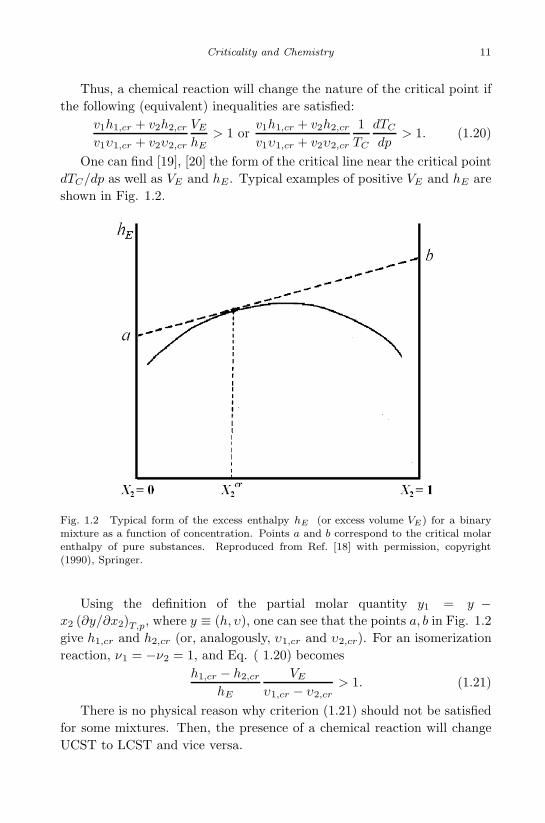
One can find [19], [20] the form of the critical line near the critical pointdTC/dp as well as VE and hE . Typical examples of positive VE and hE areshown in Fig. 1.2.
Fig. 1.2 Typical form of the excess enthalpy hE (or excess volume VE) for a binarymixture as a function of concentration. Points a and b correspond to the critical molarenthalpy of pure substances. Reproduced from Ref. [18] with permission, copyright(1990), Springer.
Using the definition of the partial molar quantity y1 = y −x2 (∂y/∂x2)T,p, where y ≡ (h, υ), one can see that the points a, b in Fig. 1.2give h1,cr and h2,cr (or, analogously, υ1,cr and υ2,cr). For an isomerizationreaction, ν1 = −ν2 = 1, and Eq. ( 1.20) becomes
h1,cr − h2,cr
hE
VE
υ1,cr − υ2,cr> 1. (1.21)
There is no physical reason why criterion (1.21) should not be satisfiedfor some mixtures. Then, the presence of a chemical reaction will changeUCST to LCST and vice versa.
September 11, 2009 10:7 World Scientific Book - 9in x 6in General-nn
12 Chemistry versus Physics: Chemical Reactions near Critical Points
1.3 Analogy between critical phenomena and the instabilityof chemical reactions
Critical phenomena describe the behavior of closed thermodynamic systemswhereas chemical reactions occur in the systems open to matter transportfrom the environment. The former are described by the well-known Gibbstechnique, but there is no universal approach to non-equilibrium chemicalreactions which are defined by the equation of the reaction rate. However,as already mentioned in the Introduction, there is a close analogy betweenthese two phenomena (in fact, article [21] is entitled “Chemical instabilitiesas critical phenomena”).
One distinguishes between phase transitions of first and second orders.First-order transitions involve a discontinuity in the state of the system,and, as a result, a discontinuity in the thermodynamic variables such asentropy, volume, internal energy (first derivatives of the thermodynamicpotential). In second-order phase transitions, these variables change con-tinuously while their derivatives, which are the second derivatives of thethermodynamic potentials (specific heat, thermal expansion, compressibil-ity), are discontinuous. Analogously, in the theory of instability of non-linear differential equations, which describe the rate of chemical reactions,one distinguishes between hard and soft transitions. These are similar innature to first-order and second-order phase transitions [22].
As an example, consider the following chemical reactions [23]
A+ 2Xk1
�k2
3X ; Ak3
�k4
X. (1.22)
These rate equations describe the conversion of the initial reactant A intoX by two parallel processes: a simple monomolecular degradation or anautocatalytic trimolecular reaction. Both these reactions are reversible withreaction constants ki, i = 1, . . . , 4. The system is open to interaction withan external reservoir of reactant A, so that the concentration of A remainsconstant. The macroscopic equation for the number of molecules X has thefollowing form
dX
dt= −k2X
3 + k1AX2 − k4X + k3A. (1.23)
The solution of Eq. (1.23) with the initial condition X(0) = X0 is(X −X1
X0 +X1
)k3−k2 ( X −X2
X0 −X2
)k1−k3 ( X −X3
X0 −X3
)k2−k1
= exp [−k2 (X1 −X2) (X2 −X3) (X3 −X1) t] (1.24)

September 11, 2009 10:7 World Scientific Book - 9in x 6in General-nn
Criticality and Chemistry 13
where X1, X2 and X3 are the three roots of
k2X3 − k1AX
2 + k4X − k3A = 0 (1.25)
with X3 ≥ X2 ≥ X1. The steady state solutions Xs of Eq. ( 1.24) are
Xs = X1 for X0 < X2;
Xs = X2 for X0 = X2; (1.26)
Xs = X3 for X0 > X2.
Stability analysis shows that the solution X2 is unstable with respect tosmall perturbations, whereas the solutionsX1 andX3 are stable. Moreover,it follows from Eq. (1.26) that hysteresis may occur as X is varied [23]. Thelast two results are typical of equilibrium phenomena which are describednear the liquid-gas critical point by the classical equation of state, say,the van der Waals equation of the form (1.25). This establishes the linkbetween first-order phase transitions in equilibrium systems and so-calledhard transitions in reactive systems.
As an example of different behavior, consider the chemical reaction
A+ C +X � A+ 2X ; X → Y +B (1.27)
where the second reverse reaction is neglected. The rate equation for thenumber of molecules X has the following form
dX
dt= −AX2 + (AC − 1)X (1.28)
or, introducing τ = At and λ = (AC − 1) /A,
dX
dτ= −X2 + λX. (1.29)
The solution of this equation has the typical features of second-orderphase transitions: the soft transition points Xs (λ) are continuous at thetransition point λ = 0, but the derivatives are not.
The foregoing equations have to be generalized to include fluctuationsfrom the steady state. No first-principle microscopic theory exists for fluctu-ations in reactive chemical systems. One usually uses a phenomenologicalmaster equation based on the macroscopic rate equations or a Langevinequation obtained by adding a stochastic term to the rate equations. Thedetails can be found in [22]. Here we bring a fascinating example of theinfluence of noise on the chemical reaction [24], which is illustrated bythe so-called ecological model. In this model, one considers two biologicalspecies with densities n1 (t) and n2 (t), which decrease with rates a1 and
September 11, 2009 10:7 World Scientific Book - 9in x 6in General-nn
14 Chemistry versus Physics: Chemical Reactions near Critical Points
a2 and compete with rates b1 and b2 for the same renewable food m. Thebirth-death equations for these species have the following form
dn1
dt= (b1m− a1)n1;
dn2
dt= (b2m− a2)n2. (1.30)
The amount of food decreases both naturally (at a rate c), and accordingto Eq. (1.30). Assume that the amount m of the food increases at rate q,i.e.,
dm
dt= q − cm− d1n1 − d2n2. (1.31)
Assume now that the species n1 is strong and species n2 is weak, whichoccurs when the ratio a1/b1 is smaller than both a2/b2 and q/c. Under theseconditions, the asymptotic t→∞ solutions of Eqs. (1.30) and (1.31) are
m =a1
b1; n2 = 0; n1 =
qb1 − ca1
b1d1(1.32)
which means that in the long run, the strong species survives and the weakspecies becomes extinct. The question arises regarding which changes canhelp the weak species to survive. One can easily see [24] that if one al-lows the food growth rate q to fluctuate in time (replacing q in Eq. (1.31)by q + f (t) with 〈f〉 = 0) or to allow the weak (but not the strong!)species to be mobile (adding the diffusive term D∇2n2 term in the secondof Eqs. (1.30)), the weak species will finally become extinct. This resultcan be formulated as the “ecological theorem”: the long-term coexistenceof two species relying on the same renewable resources is impossible. How-ever, it has been shown [24] that if both these factors occur together withnot-too-small food growth fluctuations, the corrected equations (1.30) and(1.31) have non-zero asymptotic solutions for both n1 and n2. This resulthas an important ecological interpretation. In a fluctuating environment,high mobility gives an evolutionary advantage that makes possible the co-existence of weak and strong species. The individuals of the mobile weakspecies survive since they can utilize the food growth rate fluctuations moreeffectively.
The effect outlined above, which is called a “noise-induced phase tran-sition” [25], also occurs in systems undergoing chemical reactions [24], aswell as in many other phenomena.
September 11, 2009 10:7 World Scientific Book - 9in x 6in General-nn
Chapter 2
Effect of Criticality on ChemicalReaction
2.1 The effect of pressure on the equilibrium constant andrate of reaction
Dozens of experimental results for different chemical reactions (solutes)occurring in different near-critical substances (solvents) have been reportedin the chemical literature. One such example is the tautomeric equilibriumin supercritical 1,1-difluoroethane [26], where the equilibrium rate constantincreased four-fold for a small pressure change of 4 MPa. Such a substantialincrease of the reaction rate by small variations of pressure has also beenfound [27] in styrene hydroformylation in supercritical CO2. One furtherexample is the decomposition reaction of 2,2-isobutyronitrile in mixed CO2-ethanol solvent [28], where a 70–80% increase of the reaction rate near thecritical point resulted from a small pressure change, whereas outside thecritical region, the reaction rate is nearly independent of pressure.
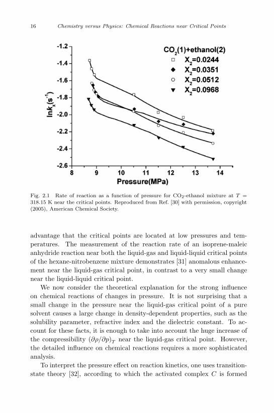
There are many experimental data concerning the Diels-Alder reaction[29], [30], one of the most interesting and useful reactions in organic chem-istry and often used for the synthesis of six-membered rings. The discover-ers of this reaction were awarded the Nobel Prize in Chemistry in 1950 “fortheir discovery and development of diene synthesis”. In Wikipedia thisreaction is considered the “Mona Lisa” of reactions in organic chemistrysince it requires very little energy to create very useful cyclohexane rings.The Deals-Alder reaction has been studied both near the liquid-gas criticalpoint of water, CO2 and SF6, as well as near the critical point of binarymixtures, such as CO2 + ethanol or CO2 + hexane. In Fig. 2.1, we show[30] the dramatic increase of the reaction rate of the CO2+ ethanol mixtureas the pressure approaches the critical point for composition.
From a technological point of view, the CO2 + ethanol mixture has the
15
September 11, 2009 10:7 World Scientific Book - 9in x 6in General-nn
16 Chemistry versus Physics: Chemical Reactions near Critical Points
Fig. 2.1 Rate of reaction as a function of pressure for CO2-ethanol mixture at T =318.15 K near the critical points. Reproduced from Ref. [30] with permission, copyright(2005), American Chemical Society.
advantage that the critical points are located at low pressures and tem-peratures. The measurement of the reaction rate of an isoprene-maleicanhydride reaction near both the liquid-gas and liquid-liquid critical pointsof the hexane-nitrobenzene mixture demonstrates [31] anomalous enhance-ment near the liquid-gas critical point, in contrast to a very small changenear the liquid-liquid critical point.
We now consider the theoretical explanation for the strong influenceon chemical reactions of changes in pressure. It is not surprising that asmall change in the pressure near the liquid-gas critical point of a puresolvent causes a large change in density-dependent properties, such as thesolubility parameter, refractive index and the dielectric constant. To ac-count for these facts, it is enough to take into account the huge increase ofthe compressibility (∂ρ/∂p)T near the liquid-gas critical point. However,the detailed influence on chemical reactions requires a more sophisticatedanalysis.
To interpret the pressure effect on reaction kinetics, one uses transition-state theory [32], according to which the activated complex C is formed
September 11, 2009 10:7 World Scientific Book - 9in x 6in General-nn
Effect of Criticality on Chemical Reaction 17
through the bimolecular reaction, expressed as
A+ B ←→ C → P (2.1)
where A and B are the reactants and P is the product. The pressuredependence of the rate constant K, expressed in mole fraction units, isgiven by
RT∂ lnK∂p
= −∆V ∗ ≡ VC − VA − VB (2.2)
where ∆V ∗ is the apparent activation volume created from the partial molarvolumes Vi of component i. Being negative, partial molar volumes dramat-ically increase upon approaching the critical points, peaking at values of−15, 000 cm3/gmol [33] compared with 5− 10 cm3/gmol far from the crit-ical point. The large values of the partial molar volumes near the criticalpoints of maximum compressibility are evident from the thermodynamicrelation
Vi = υkTn
(∂p
∂ni
)T,V,nj �=i
(2.3)
where kT is the isothermal compressibility of pure solvent, υ is the molarvolume of the solvent, ni is the number of moles of component i, and n isthe total number of moles of the mixture. Moreover, the limiting value Vcr
of the partial molar volumes at the critical point is path-dependent. Whenthe critical point is approached from above, the coexistence curve of thebinary mixture SF6 -CO2, Vcr = −230 cm3/gmol and along the isothermal-isochoric path Vcr = −40 cm3/gmol, whereas Vcr of pure SF6 equals 198cm3/gmol.
2.2 Effect of phase transformations on chemistry
One form of the interplay between chemical reactions and phase trans-formations is the change of a slow reaction in a liquid mixture in whichthe transition from the two-phase to the one-phase region results from thechange of composition during the reaction. The reaction rate was deter-mined [34] by measuring the heat production w (t) as a function of timewith a heat flow calorimeter. Thus, the chemical reaction itself serves asa probe for obtaining information about critical phenomena. There are anumber of requirements for the selection of a suitable chemical reaction:
1. It must start in the two-phase region and end in the one-phase regionor vice versa.
September 11, 2009 10:7 World Scientific Book - 9in x 6in General-nn
18 Chemistry versus Physics: Chemical Reactions near Critical Points
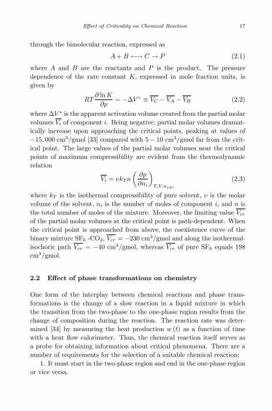
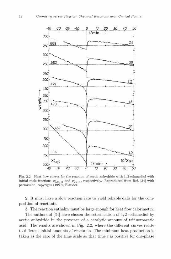
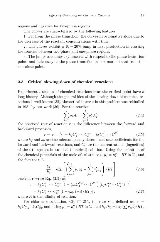
Fig. 2.2 Heat flow curves for the reaction of acetic anhydride with 1, 2-ethanediol withinitial mole fractions x0
AC2O and x0TF A, respectively. Reproduced from Ref. [34] with
permission, copyright (1989), Elsevier.
2. It must have a slow reaction rate to yield reliable data for the com-position of reactants.
3. The reaction enthalpy must be large enough for heat flow calorimetry.The authors of [34] have chosen the esterification of 1, 2 -ethanediol by
acetic anhydride in the presence of a catalytic amount of trifluoroaceticacid. The results are shown in Fig. 2.2, where the different curves relateto different initial amounts of reactants. The minimum heat production istaken as the zero of the time scale so that time t is positive for one-phase
September 11, 2009 10:7 World Scientific Book - 9in x 6in General-nn
Effect of Criticality on Chemical Reaction 19
regions and negative for two-phase regions.The curves are characterized by the following features:1. Far from the phase transition, the curves have negative slope due to
the decrease of the reactant concentrations with time.2. The curves exhibit a 10 − 20% jump in heat production in crossing
the frontier between two-phase and one-phase regions.3. The jumps are almost symmetric with respect to the phase transition
point, and fade away as the phase transition occurs more distant from theconsolute point.
2.3 Critical slowing-down of chemical reactions
Experimental studies of chemical reactions near the critical point have along history. Although the general idea of the slowing-down of chemical re-actions is well-known [35], theoretical interest in this problem was rekindledin 1981 by our work [36]. For the reaction
k∑i=1
νiAi =l∑
j=1
ν ′jA′j , (2.4)
the observed rate of reaction r is the difference between the forward andbackward processes,
r = −→r −←−r = kfCν11 · · ·Cνk
k − kbCν′1
1 · · ·Cν′l
l (2.5)where kf and kb are the microscopically determined rate coefficients for theforward and backward reactions, and Ci are the concentrations (fugacities)of the i-th species in an ideal (nonideal) solution. Using the definition ofthe chemical potentials of the mole of substance i, µi = µ0
i +RT lnCi, andthe fact that [3]
kf
kb= exp
k∑i=1
νiµ0i −
l∑j=1
ν′jµ0j
/RT
(2.6)
one can rewrite Eq. (2.5) asr = kfC
ν11 · · · Cνk
k
[1− (kbC
ν1′1 · · · Cνl′
l
)(kfC
ν11 · · ·Cνk
k )−1]
= kfCν11 · · ·Cνk
k [1− exp (−A/RT )] , (2.7)where A is the affinity of reaction.
For chlorine dissociation, Cl2 � 2Cl, the rate r is defined as r =kfCCl2−kbC
2Cl, and, using µi = µ0
i +RT lnCi, and kf/kb = exp∑νiµ
0i /RT ,
September 11, 2009 10:7 World Scientific Book - 9in x 6in General-nn
20 Chemistry versus Physics: Chemical Reactions near Critical Points
one gets
r = kfCCl2
[1− exp
(− A
RT
)]. (2.8)
Equation (2.8) implies that, in general, the rate of reaction r is a nonlin-ear function of A. However, at equilibrium, A = 0, and for small deviationsfrom equilibrium, A/RT << 1, Eq. (2.7) takes the following form,
r = LA = L
(∂A
∂ξ
)T, p
(ξ − ξeq
)+ · · · (2.9)
where L = kfCν11 · · · Cνk
k /RT . Therefore, for small deviations from equi-librium, at fixed temperature and pressure, one can restrict ourselves to thefirst term in the expansion of the affinity A (T, p, ξ) in terms of the extentof reaction ξ.
Another way to obtain Eq. (2.9) is to note that at equilibrium, wherethe extent of reaction is equal to ξeq, both dξ/dt and A vanish, and onegets
dξ
dt= L
(∂A
∂ξ
)T,p
(ξ − ξeq
). (2.10)
A detailed analysis of Eq. (2.10) has been performed [37]. Beforediscussing this work, one needs to recall some general thermodynamicideas. The thermodynamic state of a one-component, one-phase systemis determined by two variables, say, temperature and pressure. Similarly,the state of an n-component, one-phase system is determined by n+1 vari-ables. These could be the temperature T and the chemical potential of eachcomponent µi (i = 1, 2, . . . , n).
As a function of these “field” variables, the free energy G has the fol-lowing form
G = G (T, µ1...µn) . (2.11)
However, for a reactive system, the chemical potentials are not independent.According to the law of mass action in equilibrium,
A ≡n∑
i=1
νiµi = 0. (2.12)
The unconstrained free energy G can be written as
G (T, µ1...µn) = G (T, µ1...µn) + ξ
n∑i=1
νiµi (2.13)
September 11, 2009 10:7 World Scientific Book - 9in x 6in General-nn
Effect of Criticality on Chemical Reaction 21
where ξ is a Lagrange multiplier. By differentiating Eq. (2.13) with respectto µi, one obtains the particle number densities
ni = n0i + νiξ. (2.14)
Equation (2.14) implies that for a given system (with initial n0i ), the
change in ni is completely determined by the extent ξ of the reaction. Forgiven T and p, the latter quantity defines the trajectories of all possiblethermodynamic states of a system in n-dimensional phase space. However,the complete stability analysis, at given T and p, requires taking into ac-count all possible changes of ni coming both from n0
i and ξ in Eq. (2.14).In multicomponent systems, the stability with respect to diffusion is bro-ken before the thermal or mechanical stability. In terms of the Gibbs freeenergy G (T, p, n1...nn) , the condition for diffusion stability for given T andp has the form
d2G =∑i,j
dniµijdnj > 0; µij ≡ ∂µi/∂nj. (2.15)
One can easily show [3] that the matrix µij is semipositive, i.e., thedeterminant of the matrix µij vanishes, which means that the rank of µij
is equal to n − 1, and all the eigenvalues of µij but one are positive. LetN0
j be the eigenvector corresponding to eigenvalue zero,∑j
µijN0j = 0. (2.16)
Equation (2.16) is the Gibbs-Duhem relation, which has the simple phys-ical meaning of invariance with respect to proportional change of all particlenumbers. On substituting (2.14) into (2.15), one obtains
d2G =∑i,j
[dn0
iµijdn0j + 2dn0
iµijνjdξ + νiµijνj (dξ)2]> 0. (2.17)
The form q ≡ ∑i,j xiµijxj vanishes only when the determinant of thematrix µij vanishes (however, the opposite is not true, namely, for zerodeterminant of the matrix, q may remain positive). Therefore, the exis-tence of a chemical reaction does not change the stability conditions. Theequivalence of the stability conditions with respect to diffusion becomes evi-dent when one considers [3] these conditions as resulting from homogeneousand nonhomogeneous perturbations of an initially homogeneous system.
On the critical hypersurface, the expression (2.15) vanishes, i.e., newzero eigenvalues of µij appear which correspond to the eigenvector Nj sat-isfying ∑
j
µijNj = 0. (2.18)
September 11, 2009 10:7 World Scientific Book - 9in x 6in General-nn
22 Chemistry versus Physics: Chemical Reactions near Critical Points
Among all points on the critical hypersurface, those worthy of notice occurwhere the condition (2.15) is violated, and also∑
i,j
νiµijνj = 0. (2.19)
According to Eq. (2.17), this sum equals (dA/dξ)T,p, which, according toEq. (2.9), determines the slowing-down of chemical reactions.
Let us now return [37] to the main point — the comparison of Eqs.(2.16), (2.18), and (2.19), which shows that the condition (2.19) for criticalslowing-down will be satisfied if and only if
νi = αNi + βN0i (2.20)
where α and β are arbitrary constants. There are n − 2 constraints in(2.20), equal to the rank of the matrix µij on the critical hypersurface.Together with two critical conditions, they define n conditions on n + 1independent variables. Therefore, there is one free parameter, which isfixed by the law of mass action. As a result, slowing-down may appearonly at an isolated point on the critical hypersurface provided that allthe constraints are compatible. Each chemical reaction decreases by unitythe dimension of the critical hypersurface. For an n-component systemwith n− 1 chemical reactions (for example, a binary mixture with a singlechemical reaction), the only existing critical point will be where slowing-down occurs. For an n-component mixture with fewer than n− 1 chemicalreactions, the chemical instability point will be an isolated point on thecritical hypersurface, which makes experimental verification very difficult.However, in addition to a binary mixture with a single chemical reaction,slowing-down is also very probable [37] for reactions in multicomponentsystems involving the separation of slightly-dissolved substances from asolvent.
Another attack on the slowing-down problem is the general Griffiths-Wheeler method [38] of estimating the singularity of thermodynamic deriva-tives at the critical points. Indeed, according to Eq. (2.9), slowing-down isdetermined by the thermodynamic derivative (dA/dξ)T,p, and the questionarises whether this derivative has the singularity at the critical point. Grif-fiths and Wheeler [38] divide all thermodynamic variables into two classes:“fields”and “densities”. The fields (temperature, pressure, chemical poten-tials of the components) are the same in all phases coexisting in equilibrium,whereas the densities (volume, entropy, concentrations of chemical compo-nents, extents of reactions) have different values in each coexisting phase.The power of the singularity of the thermodynamic derivatives depends on
September 11, 2009 10:7 World Scientific Book - 9in x 6in General-nn
Effect of Criticality on Chemical Reaction 23
the type of variables which are kept constant under the given experimentalconditions [38]. When the experimental conditions are such that only fieldvariables are fixed, with no fixed density variables, then the derivative ofa field with respect to a density, such as (∂A/∂ξ)eq , will approach zeroas |T − Tcr|x with a “strong” critical index x of order unity. However, ifamong the fixed variables there is one density variable, the critical indexx is “weak” (of order 0.1). Finally, if two or more density variables arefixed, then x = 0, and the derivatives will be continuous. Applying theGriffiths-Wheeler rule to chemical reactions near the critical points, onehas to calculate the number of fixed densities. The latter will include allinert components which are not participating in any chemical reaction.
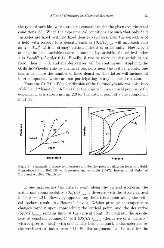
From the Griffiths-Wheeler division of the thermodynamic variables into“field” and “density”, it follows that the approach to a critical point is path-dependent, as is shown in Fig. 2.3 for the critical point of a one-componentfluid [39].
Fig. 2.3 Schematic pressure-temperature and density-pressure diagram for a pure fluid.Reproduced from Ref. [39] with permission, copyright (1987), International Union ofPure and Applied Chemistry.
If one approaches the critical point along the critical isotherm, theisothermal compressibility, (∂ρ/∂p)T=TC
, diverges with the strong criticalindex x = 1.24. However, approaching the critical point along the criti-cal isochore results in different behavior. Neither pressure or temperaturechanges rapidly upon approaching the critical point, and the derivative(∂p/∂T )υ=υC
remains finite at the critical point. By contrast, the specificheat at constant volume, Cv ≡ T (∂S/∂T )v=vcr
(derivative of a “density”with respect to “field” with one density held constant), is characterized bythe weak critical index x = 0.11. Similar arguments can be used for the
September 11, 2009 10:7 World Scientific Book - 9in x 6in General-nn
24 Chemistry versus Physics: Chemical Reactions near Critical Points
analysis of the thermodynamic variables near the critical points in many-component systems.
The preceding thermodynamic analysis is not complete, for the followingreason. Only homogeneous changes of the extent of reaction ξ are allowedby Eq. (2.9). However, if a system is large enough, the k -dependentchanges connected with sound, heat or diffusion modes become important[40]. Indeed, the relaxation rates of the latter processes will become smallerfor some small wavenumber k than the fixed k -independent rate of thechemical reaction. The general mean-field approach, which goes back to[35], is the straightforward generalization of (2.9). On the left-hand sideof the equation, instead of ξ, appears the column matrix of the density-type variables x, and instead of A, their conjugate fields appear (pressure-density, chemical potentials-concentrations, temperature-entropy, etc.)
iωx (k, ω) = L (k)X (k, ω) . (2.21)
The field variables X are related, in turn, to the density variables x bythe susceptibility matrix χ−1 byX (k, ω) = χ (k)−1
x (k, ω) (the constituentequation), leading to
iωx (k, ω) = L (k)χ (k)−1x (k, ω) ≡Mx (k, ω) . (2.22)
The matrix M = L (k)χ (k)−1 is the hydrodynamic matrix, which we willanalyze in detail when we consider the hydrodynamic equations for a reac-tive system.
As emphasized in [40], Eq. (2.21) shows that the relaxation of theextent of reaction ξ arises not only through the chemical processes (with
characteristic time τ ≡[L (∂A/∂ξ)eq
]−1
away from the critical point),but also through diffusion and heat conductivity (with characteristic times(Dk2
)−1 and(λk2/ρCp
)−1, respectively). Therefore, one must compare therelaxation times or characteristic lengths (inverse wavenumbers) in order todetermine which quantity should be considered constant. As we have seen,this is of crucial importance for the analysis of slowing-down processes.
Let us define two characteristic lengths by k−2C = Dτ and k−2
H =λτ/ρCp, where, generally, k−1
H >> k−1C . Values of the wavenumbers k fall
into three intervals: k < kH , kH < k < kC , and k > kC . In the first inter-val, the chemical reaction is more rapid than both heat conductivity anddiffusion, whereas in the third interval, diffusion dominates the chemicalrelaxation. Only for processes with wavenumbers located in the “window”between kH and kC is the relaxation dominated by chemistry. For typicalvalues of the heat conductivity, λ/ρCp = 0.1 cm2/s, the diffusion constant
September 11, 2009 10:7 World Scientific Book - 9in x 6in General-nn
Effect of Criticality on Chemical Reaction 25
D = 10−5 cm2/s, and for a reaction rate τ−1 = 120 Hz, we have kH = 103
cm−1 and kC = 105 cm−1. Therefore, light scattering experiments withk ≈ 104 cm−1 at different temperatures in the vicinity of the critical tem-perature provides evidence for the slowing-down of chemical reactions nearthe critical points.
Note that the “slowing-down” of the chemical reaction does not implythat the forward or backward reaction is slowed down. It is the measuredrate, which is the net difference between the forward and backward reac-tions, which is affected by criticality. In fact, condition (2.19), which is re-ally (∂A/∂ξ)T,p ≈ 0, means that the system becomes indifferent to changesin the species concentration. In equilibrium, when A = 0, the reaction isbalanced and the measured rate is zero. Usually, a change of ξ from ξeq
builds up an affinity A �= 0 which acts as a driving force to restore theequilibrium. However, due to the thermodynamic properties in the criticalregion, a change in ξ does not create a restoring force (i.e., affinity), andthe reaction continues to be balanced even though ξ �= ξeq. That is, therate continues to be zero. In other words, the physical explanation of theslowing-down of the chemical reaction is the same as the explanation of dif-fusion near the critical points of nonreactive systems, where the vanishingof diffusion does not mean that the individual particles are slowing-down.The only difference is that the chemical perturbation is homogeneous, incontrast to the inhomogeneous diffusion changes.
All the above considerations hold for a two-component mixture with asingle chemical reaction. If the system hasm reactants and n products, thenthere arem+n−2 conserved variables. If allm+n species in the system takepart in the reaction, then the reaction can slow-down strongly form+n < 3,weakly for m + n = 3, and not at all for m + n > 3. Therefore, for morecomplicated systems than a binary mixture, strong critical slowing-downis not likely to occur in the usual experimental situation. The additionalfactor which has to be taken into account in analyzing an experiment,is the path of approach to the critical point (at some fixed parameter(s),along the coexistence curve, etc.), since the behavior of the thermodynamicderivatives is path-dependent.
2.4 Hydrodynamic equations of reactive binary mixture:piston effect
The slowing-down of the dynamic processes near the liquid-gas criticalpoints, considered in the previous section, is the hallmark of critical phe-
September 11, 2009 10:7 World Scientific Book - 9in x 6in General-nn
26 Chemistry versus Physics: Chemical Reactions near Critical Points
nomena. It is precisely this fact which makes it so difficult to obtain reliableequilibrium experimental data near the critical points.
However, the very interesting phenomenon of the speeding-up of dy-namic processes in critical fluids at constant volume, as opposed to theirslowing-down, was predicted theoretically [41], and afterwards found ex-perimentally [42]. The usual experimental set-up is a fluid-filled closed cell.After changing the temperature at the bottom or around the cell, one waitsfor the establishment of thermal equilibrium inside the cell. The slow diffu-sive heat propagation is responsible for the critical slowing-down. However,fast thermal equilibrium is established through the thermo-acoustic effect[41], where the temperature change at the surface induces acoustic waveswhich lead to a fast change of the pressure, and hence, of the tempera-ture everywhere in the fluid. This is also called the “piston effect”, sincethe thermal boundary layer generated near the heated bottom of the cellproduces, like a piston, the pressure on the fluid restricted to a constantvolume.
The speeding-up of an interface reaction, which is immediately evidentfrom the piston effect, has been explained in [43]. There are also otherexplanations for the speeding-up of chemical reactions near critical pointsbased on specific properties, such as appearance of the soft modes in thevibrational spectrum of solids [44], reduction of the H-bond strength in wa-ter [45], and the solid-solvent clustering mechanism [46]. We shall considersome special examples.
2.4.1 Heterogeneous reactions in near-critical systems
The interface reaction that takes place in a supercritical phase may be citedas an illustration of an immediate influence of the piston effect on the fluxof matter at the interface, leading to the speeding-up of the chemical re-action [43], [47]. Such speeding-up manifests itself in the strong corrosionobserved in supercritical fluid containers [48]. Two factors — the sensitivityof solubility to the small changes of pressure, induced by the piston effect,and the supercritical hydrodynamics — affect the absorption-desorptionreaction taking place between a solid interface and an active component ina dilute binary supercritical mixture. The method of matched asymptoticexpansion has been used [43] for the solution of the simplified system ofone-dimensional hydrodynamic equations with a van der Waals equation ofstate and linear mixing rules. The asymptotic analysis shows the couplingbetween the piston effect and an interface reaction, which — for some ini-
September 11, 2009 10:7 World Scientific Book - 9in x 6in General-nn
Effect of Criticality on Chemical Reaction 27
tial conditions — leads to a strong increase of the flux of matter and theintensification of a reaction.
More detailed analysis has been performed [47]. The numerical solutionof the full hydrodynamic equations based on the finite volume approxima-tion has been carried out for a system involving a small amount of naphtha-lene dissolved in supercritical CO2 located between two infinite solid platesmade of pure solid naphthalene and able to absorb or desorb naphthalenefrom the fluid. The fluid is initially at rest. The temperature of one of theplates is then gradually increased while the other plate is kept at the initialtemperature. Due to the small amount of naphthalene in solution, for nu-merical simulation one can use the parameters of pure CO2. The results ofthe analysis show that there are three mechanisms for the increase of themass fractions of the naphthalene w at the solid interface:
1. The critical behavior of the solute solubility through the large valuesof (∂w/∂p)T , and (at the heated plate) of (∂w/∂T )p.
2. The strong compressibility of the supercritical fluid through thederivative (∂w/∂p)T , and the piston effect that results through the pressurevariation.
3. The strong dilatability expressed by the large derivative (∂w/∂T )pand through the density variation.
The piston effect, coupled with the critical behavior of the solute sol-ubility with respect to pressure, is the leading mechanism governing themass fraction of naphthalene at the isothermal plate [47]. Similar simu-lations have been performed with cooling, rather than heating one of theplates, and a similar phenomenon was observed: the strong decrease of thepressure caused by the piston effect leads to a strong decrease of the massfraction of naphthalene at the isothermal plate.
In the next section, we carry out a phenomenological analysis based onthe full hydrodynamic equations in a reactive mixture [49], [50].
2.4.2 Dynamics of chemical reactions
There are two different phenomenological ways to describe chemical reac-tions: the hydrodynamic approach, used by physicists and which we usehere, and the rate equations, used mostly by chemists.
We consider an isomerization reaction between two species which is de-scribed by the equation A � B. This simple example of a chemical reactioncan be easily generalized to more complex reactions. The question arises asto the choice of the thermodynamic variables which characterize the binary
September 11, 2009 10:7 World Scientific Book - 9in x 6in General-nn
28 Chemistry versus Physics: Chemical Reactions near Critical Points
mixture. A one-component thermodynamic system is characterized by twoparameters, such as pressure and temperature. For a binary mixture, onehas to add one additional parameter, such as the concentration ξ of one ofthe components, which will also describe a chemical reaction. Indeed, for bi-nary mixtures, the chemical potential µ, defined [4] as µ = µ1/m1−µ2/m2,where m1 and m2 are the molecular masses of the components, is propor-tional to the affinity A = µ1ν1 − µ2ν2 of the chemical reaction since thestoichiometric coefficients ν1, ν2 are inversely proportional to the molecularmasses of the species. Thus, one can choose the mass fraction of one com-ponent as the progressive variable ξ of a chemical reaction. The dynamicbehavior of a reactive binary mixture, described by the hydrodynamic equa-tions, will contain a fourth variable, which for an isotropic system can bechosen as div (v).
As discussed in the previous section, near equilibrium in the linear ap-proximation, one obtains
dξ
dt= −L0A = −L0
(dA
dξ
)eq
(ξ − ξeq
). (2.23)
The subscript eq means that the thermodynamic derivative is calcu-lated in equilibrium, and L0 is the Onsager coefficient. The quantity[Lo (∂A/∂ξ)eq
]−1
is the characteristic time of the chemical reaction de-scribed by the phenomenological equation (2.23). In real system, however,the chemical reaction occurs in some media, and the “chemical” mode in-teracts with other hydrodynamic modes, such as diffusive, viscous and heatconductive modes, i.e., one has to consider the entire system of hydro-dynamic equations. This requires calculating the “renormalized” Onsagercoefficient L due to the interaction with the hydrodynamic modes (“modecoupling”). In equilibrium statistical mechanics, there exists a general pro-cedure for calculating the thermodynamic quantities, which goes back toGibbs. No such systematic procedure exists in non-equilibrium statisti-cal mechanics. However, for non-equilibrium states that are not far fromequilibrium, some general formulae do exist which connect the kinetic coeffi-cients with long-wavelength limits of the correlation functions. The Onsagercoefficient plays a role analogous to that of transport coefficients in hydro-dynamics, and both are described by the Green-Mori-Zwanzig relations[51]–[53]. The “chemical” mode is characterized by the local interactionswhereas the pure hydrodynamic modes depend upon spatial gradients. Ina real fluid, there are couplings between different modes, and the Onsager
September 11, 2009 10:7 World Scientific Book - 9in x 6in General-nn
Effect of Criticality on Chemical Reaction 29
coefficient L is defined for small wavenumbers k, as the correlation func-tion of the changes of the concentration (∂ξ/∂t)chem due to the chemicalreaction [54],
L =1
κBT0
∞∫0
dt
⟨(∂ξ
∂t
)chem
(k, t)(∂ξ
∂t
)chem
(−k, 0)⟩. (2.24)
Equation (2.24) provides the connection between the phenomenologicalOnsager coefficient and the microscopic time correlation function. First ofall, let us check that in the absence of the hydrodynamic modes, when theaffinity A depends only on the concentration ξ rather than on all thermody-namic variables, the renormalized Onsager coefficient L, defined in (2.24),reduces to the “bare” Onsager coefficient L0. Indeed, the solution of Eq.(2.23) has the form
ξ − ξeq = exp
[−L0
(dA
dξ
)eq
t
]. (2.25)
Substituting (2.23) and (2.25) into (2.24) yields
L = L20
(dA
dξ
)2
eq
1κBT0
∞∫0
dt exp
[−L0
(dA
dξ
)eq
t
]〈ξ (k, 0) ξ (−k, 0)〉 .
(2.26)
Performing the integration over t in (2.26), and taking into account[4] that the equilibrium correlation function 〈ξ (k, 0) ξ (−k, 0)〉 equalsκBT0/ (dA/dξ)eq, one immediately obtains that L = L0, as requires fora purely chemical process. In the following section, we will consider the in-fluence of the hydrodynamic modes on the renormalized Onsager coefficient.
2.4.3 Relaxation time of reactions
Consider the isomerization reaction with c1 and c2 being the mass con-centrations of substances A and B, and γij are the transition rates fromcomponent i to component j. The change of the concentration of compo-nent A caused by gain and loss to component B, is described by
dc1dt
= γ21c2 − γ12c1 = γ21 − (γ12 + γ21) c1. (2.27)
For a closed system the total number of particles is constant, c1+c2 = 1,which has been used in Eq. (2.27). This equation contains the characteristic
September 11, 2009 10:7 World Scientific Book - 9in x 6in General-nn
30 Chemistry versus Physics: Chemical Reactions near Critical Points
time of the reaction r0 which depends on the rate constants γ12 and γ21 atequilibrium,
r0 =1
γ12 + γ21
. (2.28)
At equilibrium, dc1/dt = 0, and
γ12c01 = γ21c
02. (2.29)
The kinetic processes lead to the renormalization of this characteristic time,which is described by Eq. (2.24) with a slight change in the constantcoefficient,
r =1c01c
02
∞∫0
dt
⟨(∂c
∂t
)chem
(k, t)(∂c
∂t
)chem
(−k, 0)⟩. (2.30)
If a system is open, the particles are able to enter and leave. Then, theconcentrations depend both on chemical transformations and on diffusion,and their time dependence is described by the following equations [55],
∂c1/∂t = D1∇2c1 − γ12c1 + γ21c2,
∂c2/∂t = D2∇2c1 − γ21c2 + γ12c1.(2.31)
We use the Fourier and Laplace transforms in space and time, respec-tively,
ci (k, s) =∫∫
drdt exp (−ikr) exp (−st) ci (r, t) . (2.32)
The solutions of Eqs. (2.31) are
c1 (k, s) =
(s+ k2D1 + γ21
)c1 (k, 0) + γ21c2 (k, 0)∆
,
c2 (k, s) =
(s+ k2D2 + γ12
)c2 (k, 0) + γ12c1 (k, 0)∆
,
(2.33)
where
∆ = s2 + s[(D1 +D2) k2 + γ21 + γ12
]+ k2 (D1γ12 +D2γ21) + k4D1D2. (2.34)
Multiplying Eqs. (2.33) by c1 (−k, 0) and c2 (−k, 0) and averaging, oneobtains the expressions for the matrix elements 〈ci (k, s) cj (−k, 0)〉 , for
September 11, 2009 10:7 World Scientific Book - 9in x 6in General-nn
Effect of Criticality on Chemical Reaction 31
i, j = 1, 2, as functions of the equilibrium averages 〈ci (k, 0) cj (−k, 0)〉 . Forspecial systems, such as structurally similar isomers, for which D1 = D2 ≡D, one gets
〈c1 (k, s) c1 (−k, 0)〉
=
[s+ k2D + γ21
] 〈c1 (k, 0) c1 (−k, 0)〉+ γ21 〈c2 (k, 0) c1 (−k, 0)〉s2 + s
(γ+ + 2k2D
)+ k2γ+D + k4D2
, (2.35)
〈c2 (k, s) c2 (−k, 0)〉
=
[s+ k2D + γ12
] 〈c2 (k, 0) c2 (−k, 0)〉+ γ12 〈c1 (k, 0) c2 (−k, 0)〉s2 + s
(γ+ + 2k2D
)+ k2γ+D + k4D2
, (2.36)
〈c1 (k, s) c2 (−k, 0)〉
=
[s+ k2D + γ21
] 〈c1 (k, 0) c2 (−k, 0)〉+ γ21 〈c2 (k, 0) c2 (−k, 0)〉s2 + s
(γ+ + 2k2D
)+ k2γ+D + k4D2
, (2.37)
〈c2 (k, s) c1 (−k, 0)〉
=
[s+ k2D + γ12
] 〈c2 (k, 0) c1 (−k, 0)〉+ γ12 〈c1 (k, 0) c1 (−k, 0)〉s2 + s
(γ+ + 2k2D
)+ k2γ+D + k4D2
, (2.38)
where γ+ = γ21 + γ12.Equations (2.35)–(2.38) are simplified when both components are taken
to be ideal gases. Then, 〈ci (k, 0) cj (−k, 0)〉 = c0jδij , so that
〈c1 (k, s) c1 (−k, 0)〉
= c01s+ k2D + γ21
s2 + s (γ21 + γ12 + 2k2D) + k2γ+D + k4D2, (2.39)
〈c2 (k, s) c2 (−k, 0)〉
= c02
[s+ k2D + γ12
]s2 + s (γ21 + γ12 + 2k2D) + k2γ+D + k4D2
, (2.40)
〈c1 (k, s) c2 (−k, 0)〉
= c02γ21
s2 + s (γ21 + γ12 + 2k2D) + k2γ+D + k4D2, (2.41)
〈c2 (k, s) c1 (−k, 0)〉
= c01γ12
s2 + s (γ21 + γ12 + 2k2D) + k2γ+D + k4D2. (2.42)
September 11, 2009 10:7 World Scientific Book - 9in x 6in General-nn
32 Chemistry versus Physics: Chemical Reactions near Critical Points
Substituting into (2.30) the expression (∂c/dt)chem = γ21c2−γ12c1, oneobtains
r =1c01c
02
∞∫0
dt
∞∫0
ds exp (st) {γ212 〈c1 (k, s) c1 (−k, 0)〉
+ γ221 〈c2 (k, s) c2 (−k, 0)〉
− γ12γ21 [〈c1 (k, s) c2 (−k, 0)〉+ 〈c2 (k, s) c1 (−k, 0)〉]} (2.43)
which takes the following form after using Eqs. (2.39)–(2.42),
r =
(γ2
12c01 + γ2
21c02
)c01c
02
×∞∫0
dt
∞∫0
ds
(s+ k2D
)exp (st)
s2 + s(γ+ + 2k2D
)+ k2γ+D + k4D2
. (2.44)
To perform the inverse Laplace transformation on Eq. (2.44), one needsthe roots of the denominator,
s1 = −k2D; s2 = −k2D − γ+. (2.45)
Integrating over s yields
r =γ2
12c01 + γ2
21c02
c01c02 (γ12 + γ21)
∞∫0
exp[− (k2D + γ+
)t]dt
=γ2
12c01 + γ2
21c02
c01c02 (γ12 + γ21) (k2D + γ21 + γ12)
(2.46)
which can be rewritten by using Eq. (2.29),
r =1
(k2D + γ21 + γ12). (2.47)
For D = 0, this solution reduces to Eq. (2.28), as required.
2.4.4 Hydrodynamic equations of a reactive binary
mixtures
The hydrodynamic equations are the conservation laws of mass, momen-tum, concentration and energy. They are the continuity equation,
dρ
dt= −div (ρv) , (2.48)
September 11, 2009 10:7 World Scientific Book - 9in x 6in General-nn
Effect of Criticality on Chemical Reaction 33
the Navier-Stokes equation,
ρdvi
dt= − ∂
∂xjσij , (2.49)
the conservation of one of the components,
dξ
dt= −div (Jξ) , (2.50)
and the conservation of energy,
dQ
dt= ρT
dS
dt= −div (Jε) . (2.51)
Just as ρv in Eq. (2.48) represents the mass flux, the terms σij , Jξ, andJε in (2.49)–(2.51) describe the stress tensor, fluxes of mass of one of thecomponents and energy, respectively. The phenomenological forms of thesequantities, which include both hydrodynamic and chemical flows, are basedon the symmetry requirements for vectors J , v and scalars ρ, ξ, S and thechemical affinity A.
The well-known expressions for hydrodynamic fluxes are [4]
(σij)hydr = δijp+ η
[∂vi
∂xj+∂vj
∂xi− 2
3δijdiv (v)
]+ δijζdiv (v) , (2.52)
(Jξ)hydr = −Dgrad (ξ)−D[kT
Tgrad (T ) +
kp
pgrad (p)
], (2.53)
(Jε)hydr = −λgrad (T )−ρD(∂A
∂ξ
)p,T
[kT grad (ξ) +
kp
pgrad (p)
]. (2.54)
The variables appearing in (2.48)–(2.54) have obvious meaning. Thecoefficient kT defines the Dufour and Soret cross-effects, whereas kp/p is apurely thermodynamic quantity defined by
kp
p=
(∂A/∂p)T,ξ
(∂A/∂ξ)p,T
. (2.55)
For small deviations from chemical equilibrium, the constitutive equa-tion takes the form (
dξ
dt
)chem
= −L0A. (2.56)
The heat change in the chemical reaction is given by
λ =∆hC
(2.57)
September 11, 2009 10:7 World Scientific Book - 9in x 6in General-nn
34 Chemistry versus Physics: Chemical Reactions near Critical Points
where C is the heat capacity, and ∆h is the change of enthalpy per unitmass of reaction. The heat flux caused by the chemical reaction is(
dQ
dt
)chem
= λL0A. (2.58)
Since ∆h is proportional to A, the λLA term in Eq. (2.58) is proportionalto A2, and can therefore be neglected for small deviations from equilibrium,as is assumed when using the hydrodynamic theory.
The phenomenological relations (2.56) and (2.52)–(2.54) are based onsymmetry considerations which — in the presence of a chemical reaction —allow the appearance of an additional visco-reactive cross effects, describedby the L1 terms. This leads to the following generalization of Eqs. (2.56)and (2.52),
(dξ
dt
)chem
= −L0A− L1div (v) (2.59)
(σij)chem = δijL1A. (2.60)
Inserting (2.53), (2.59), and (2.60) into (2.49)–(2.51), yields fourlinearized hydrodynamic equations,
∂ρ
∂t= −ρ0div (v) (2.61)
ρ0
∂v
∂t= −grad (p)+ η∇2v+
(η3
+ ζ)grad (div (v))+ρ0L1grad (A) (2.62)
∂ξ
∂t= D∇2ξ +D
(kT
T∇2T +
kp
p∇2p
)− L0A− L1div (v) (2.63)
ρT∂S
∂t= λ∇2T + ρD
(∂A
∂ξ
)p,T
(kT∇2ξ +
kp
p∇2p
)(2.64)
where ρ, p, T and ξ are the deviations of density, pressure, temperature andthe mass fraction of one of the components from their equilibrium valuesdenoted by the subscript zero. The transport coefficients in Eqs. (2.61)–(2.64) are the shear viscosity η, the bulk viscosity ς, the heat-conductivityλ, the diffusion coefficient D, the thermal-diffusion coefficient kT , and thebaro-diffusion coefficient kp.
The rigorous treatment of the correlation functions, which, accordingto Eq. (2.24), define the renormalized Onsager coefficient L, requires thatallowance be made for the symmetry properties of the variables entering the
September 11, 2009 10:7 World Scientific Book - 9in x 6in General-nn
Effect of Criticality on Chemical Reaction 35
hydrodynamic equations (2.61)–(2.64). The quantity (∂ξ/∂t)chem and thevariable div (v) are odd functions under time reversal and even functionsunder parity [36], while the other variables are either even or odd underboth symmetry operations. However, these arguments are not relevant inthe following, since we use simplified models.
Using Eq. (2.61), one can omit div (v) from Eqs. (2.62 )–(2.63), whichgives
−∂2ρ
∂t2= −∇2p− 1
ρ0
(43η + ζ
)∇2 ∂ρ
∂t+ ρ0L1∇2A (2.65)
∂ξ
∂t= D∇2ξ +D
(kT
T∇2T +
kp
p∇2p
)− L0A+
L1
ρ0
∂ρ
∂t. (2.66)
To solve Eqs. (2.64)–(2.66), we express A, T and p in terms of the vari-ables ρ, ξ, S. In equilibrium, A = 0. For small deviations from equilibrium,
A =(∂A
∂ρ
)ξ,S
ρ+(∂A
∂S
)ρ,ξ
S +(∂A
∂ξ
)S,ρ
ξ. (2.67)
Our analysis is based on the assumption of local equilibrium, i.e.,
T = (∂T/∂ρ)ξ,S ρ+ (∂T/∂S)ρ,ξ S + (∂T/∂ξ)S,ρ ξ,
p = (∂p/∂ρ)ξ,S ρ+ (∂p/∂S)ρ,ξ S + (∂p/∂ξ)S,ρ ξ.(2.68)
Inserting (2.67) and (2.68) into (2.64)–(2.66) yields [56] a quite cumber-some system of three differential equations in three variables ρ, ξ, S. TheFourier and Laplace transforms in space and time, respectively, yield thefollowing solution of these equations,
ξ (k, s) =f1 (k, s) ξ (k, 0) + f2 (k, s) ρ (k, 0) + f3 (k, s)S (k, 0)
∆, (2.69)
ρ (k, s) =f4 (k, s) ξ (k, 0) + f5 (k, s) ρ (k, 0) + f6 (k, s)S (k, 0)
∆, (2.70)
S (k, s) =f7 (k, s) ξ (k, 0) + f8 (k, s) ρ (k, 0) + f9 (k, s)S (k, 0)
∆, (2.71)
September 11, 2009 10:7 World Scientific Book - 9in x 6in General-nn
36 Chemistry versus Physics: Chemical Reactions near Critical Points
where the determinant of the coefficients in the original equations, ∆, andthe functions fi (i = 1, . . . , 9) are cumbersome combinations of the thermo-dynamic variables and transport coefficients, which can be found in [56].
The complicated hydrodynamic equations can be simplified if one ne-glects the higher terms in k2. Performing the Fourier-Laplace transformsof Eqs. (2.65) and (2.66), written in the variables ρ and ξ, one gets
K1,ρρ (k, s) +K1,ξξ (k, s)
=[s− 1
ρ0
(43η + ζ
)k2
]ρ (k, 0) + ∂ρ (k, 0) /∂t,
K2,ρρ (k, s) +K2,ξξ (k, s) = ξ (k, 0)− (L1/ρ0) ρ (k, 0) , (2.72)
where one can set ∂ρ (k, 0) /∂t = 0, and
K1,ρ = s2 + k2
[(∂p
∂ρ
)ξ,S
+(
43γ + ζ
)s
ρ0
+ ρ0L1
(∂A
∂ρ
)ξ,S
], (2.73)
K1,ξ = k2
[(∂p
∂ξ
)ρ,S
+ ρ0L1
(∂A
∂ξ
)ρ,S
], (2.74)
K2,ρ = L0
(∂A
∂ρ
)ξ,S
+Dk2
(∂ξ
∂ρ
)ξ,S
− sL1
ρ0
, (2.75)
K2,ξ = s+ k2D + L0
(∂A
∂ξ
)ρ,S
. (2.76)
The solutions of Eqs. (2.72) are
ρ (k, s)
=
{K2,ξ
[s− 1
ρ0
(43η + ζ
)k2]−K1,ξ
L1ρ0
}ρ (k, 0)−K1,ξξ (k, 0)
K1,ρK2,ξ −K2,ρK1,ξ
(2.77)
ξ (k, s)
=K1,ρ
[ξ (k, 0)− L1
ρ0ρ (k, 0)
]−K2,ρ
[s− 1
ρ0
(43η + ζ
)k2]ρ (k, 0)
K1,ρK2,ξ −K2,ρK1,ξ.
(2.78)
To lowest order in k2, Eq. (2.77) takes the following form
September 11, 2009 10:7 World Scientific Book - 9in x 6in General-nn
Effect of Criticality on Chemical Reaction 37
ρ (k, s) = sρ (k, 0){s2 +
(sk2/ρ0
)(43γ + ζ
)+[(∂p/∂ρ)ξ,S + ρ0L1 (∂A/∂ρ)ξ,S
]k2
+[(∂p/∂ξ)ξ,S + ρ0L1∂A/∂ξξ,S
] [sL1/ρ0 − L0 (∂A/∂ξ)ρ,S
]×[s+ L0 (∂A/∂ξ)ρ,S
]−1
k2
}−1
≈ sρ (k, 0)
{[s+
(k2/2ρ0
)(43γ + ζ
)]2
+[(∂p/∂ρ)ξ,S + ρ0L1 (∂A/∂ρ)ξ,S
]k2}−1
. (2.79)
The inverse Laplace transform yields
ρ (k, t) = ρ (k, 0) exp[− 1
2ρ0
(43γ + ζ
)k2t
]
× cos
[(
∂p
∂ρ
)ξ,S
+ L1
(∂A
∂ρ
)ξ,S
]1/2
kt
. (2.80)
Analogously, to lowest order in k2, one gets from Eq. (2.78),
ξ (k, t)
=[ξ (k, 0)− L1
ρ0
ρ (k, 0)]
exp
[−(Dk2 + L0
(∂A
∂ξ
)ρ,S
)t
]. (2.81)
According to Eq. (2.24), the rate of the chemical reaction is defined bythe change of concentration (∂ξ/∂t)chem due to the chemical reaction. Inthe case under consideration, this change is given by the term −L0A inEq. (2.66). Using ξ and ρ as independent variables, one gets
L =(L2
0/kBT0
) ∫ ∞
0
dt 〈A (k, t)A (−k, 0)〉
=(L2
0/kBT0
)(∂A/∂ξ)2ρ,S
∫ ∞
0
dt[〈ξ (k, t) ξ (−k, 0)〉
+ (∂ξ/∂ρ)2A,S 〈ρ (k, t) ρ (−k, 0)〉− (∂ξ/∂ρ)A,S (〈ξ (k, t)ρ (−k, 0)〉+ 〈ρ (k, t) ξ (−k, 0)〉)]. (2.82)
September 11, 2009 10:7 World Scientific Book - 9in x 6in General-nn
38 Chemistry versus Physics: Chemical Reactions near Critical Points
The correlators in Eq. (2.82) can easily be found from Eqs. (2.80) and(2.81) as functions of equilibrium correlators
〈ρ (k, 0) ρ (−k, 0)〉 = κT0ρ20 (∂p/∂ρ)−1
ξ,S ,
〈ξ (k, 0) ξ (−k, 0)〉 = κT0 (∂A/∂ξ)−1ρ,S ,
〈ξ (k, 0) ρ (−k, 0)〉 = −κT0 (∂ρ/∂A)ξ,S .
(2.83)
Finally, one obtains
L = L20 (∂A/∂ξ)2p,S
L1
ρ0
[Dk2 + L0 (∂A/∂ξ)ρ,S ]−1
+(∂ξ
∂ρ
)A,S
2 (4η/3 + ζ) ρ0
(4η/3 + ζ)2 k2 + 4[(∂p/∂ρ)ξ,S + ρ0L1 (∂A/∂ρ)ξ,S
]
×[(∂ρ/∂A)ξ,S + ρ2
0 (∂ξ/∂ρ)A,S (∂ρ/∂p)ξ,S
] . (2.84)
2.4.5 Hydrodynamic equations with statistically
independent variables
The thermodynamic variables x1, x2, . . . , xn are statistically independentif their cross-averages 〈xixj〉 vanish for i �= j, so that the probability offluctuations is given by
P (δx1, δx2, . . . , δxn) =
exp[−A1
2(δx1)
2 − A2
2(δx2)
2 − · · · − An
2(δxn)2
](2.85)
with⟨(δxi)
2⟩
= A−1i .
For a one-component system, one can choose ρ, T or p, S as statisticallyindependent variables, since 〈δρδT 〉 = 〈δpδS〉 = 0. For a many-componentsystem, there are different possibilities for choosing the set of the hydrody-namic variables x1,x2, . . . , which characterize the state of a system. Usingwell-known thermodynamic formulae [4], one can verify that there are dif-ferent sets of statistically independent variables. We have chosen the massfraction x, the pressure p, div (v) and the variable φ = Cp,xT/T0−αT p/ρ0,
where αT is the isobaric thermal expansion and Cp,x is the specific heat at

September 11, 2009 10:7 World Scientific Book - 9in x 6in General-nn
Effect of Criticality on Chemical Reaction 39
constant pressure. Another possible set of statistically independent vari-ables is the mass fraction x, the pressure p, div (v) and the reduced entropyS1 = S − (∂S/∂x)p,T x, or the temperature T, the pressure p, div (v) andthe variable φ. Note that for a chemically reactive ternary mixture, it isconvenient [57] to use the reduced entropy and the reduced concentration,
S1 = S − (∂S/∂x)p,T x1; x = x1 − (∂x1/∂x2)p,T x2. (2.86)
After performing a Fourier transform, the set of linearized hydrody-namic equations can be written symbolically in the form
d
dtN (k, t) = −M (k, t)N (k, t) (2.87)
where N (k, s) is a column vector with n hydrodynamic variables (n = 4for the case discussed below), and the form of the n ∗ n matrix M(k, s) isdefined by the hydrodynamic equations. Solutions of Eqs. (2.87) have thefollowing form
Ni (k, s) = [detM (k, s)]−1∑
j
Pij (k, s)Nj (k) , (2.88)
where the Pij are algebraic functions. From Eq. (2.88), one gets the corre-lation functions
〈Nj (k, s)Nj (−k)〉 = Pij (k, s)det M (k, s)
⟨|Nj (k)|2
⟩, (2.89)
if all Nj are statistically independent.An expression for the time-dependent correlation function is obtained
by taking the inverse Laplace transform of Eq. (2.89),
〈Nj (k, t)Nj (−k)〉 =
⟨|Nj (k)|2
⟩2π
∞∫−∞
ds exp (st)Pij (k, s)detM (k, s)
. (2.90)
To perform the integration in (2.90), one has to find the roots ofdetM (k, s).
Neglecting the visco-reactive terms (setting L1 = 0 in Eqs. (2.62)–(2.63)), one can write the complete set of linearized hydrodynamic equa-tions in the variables p, x, and div (v) and the new variable φ = Cp,xT/T0−αT p/ρ0. This choice of hydrodynamic variables has been used for non-reactive mixtures [58] , and then extended to reactive mixtures [59], [60].These equations take the following form [60], [61](
∂ρ
∂x
)p,T
∂x
∂t+(∂ρ
∂p
)x,T
∂p
∂t+
T0
Cp,x
(∂ρ
∂T
)x,p
∂φ
∂t+ ρ0div (v) = 0
(2.91)
September 11, 2009 10:7 World Scientific Book - 9in x 6in General-nn
40 Chemistry versus Physics: Chemical Reactions near Critical Points
∂div (v)∂t
= −∇2p+(
43η + ς
)∇2div (v) ; (2.92)
∂x
dt= D∇2x+D
(kp
p0+
kTαT
ρ0Cp,x
)∇2p+D
kT
Cp,x∇2φ− L0A; (2.93)
ρ0T0 (∂φ/∂t)− ρ0kT (∂A/∂x)p,T (∂x/∂t)
−T0
[αT − ρ0 (∂S/∂p)x,T
](∂p/∂t)
= λ[(T0/Cp,x)∇2φ+
(TαT /ρ0
Cp,x
)∇2p]. (2.94)
The chemical term L0A appears in Eq. (2.93). Since the affinity A
vanishes at equilibrium, one can expand A in terms of x, p, and T ,
A =(∂A
∂x
)p,T
x+(∂A
∂p
)x,T
p+(∂A
∂T
)x,p
T. (2.95)
Substituting T = T0φ/Cp,x + T0αT p/ρ0Cp,x into Eq. (2.95) yields
L0A = L0 (∂A/∂x)p,T
[x− (∂x/∂p)T,A p
− (∂x/∂T )p,A (T0φ/Cp,x + T0αT p/ρ0Cp,x)]
= L0 (∂A/∂x)p,T
{x−
[(∂x/∂p)T,A + (∂x/∂T )p,A T0αT /ρ0Cp,x
]p
− (T0/Cp,x) (∂x/∂T )p,A φ}. (2.96)
Inserting (2.96) into (2.93) gives
∂x/dt =[D∇2 − L0 (∂A/∂x)p,T
]x
+{D (kp/p0 + kTαT /ρ0Cp,x)∇2
−L0
[(∂A/∂p)x,T + (∂A/∂T )x,p T0αT /ρ0Cp,x
]}p
+[DkT
Cp,x∇2 + (∂A/∂x)p,T (∂x/∂T )p,A T0L0/Cp,x
]φ. (2.97)
September 11, 2009 10:7 World Scientific Book - 9in x 6in General-nn
Effect of Criticality on Chemical Reaction 41
Finally, inserting (2.97) into (2.94) yields
∂φ/∂t = (∂A/∂x)p,T kT /T0
[D∇2 − L0 (∂A/∂x)p,T
]x
+{(λ/ρ0Cp,x)∇2 + kT /T0
[(DkT /Cp,x) (∂A/∂x)p,T ∇2
− (T0L0/Cp,x) (∂A/∂x)2p,T (∂x/∂T )p,A
]}φ
+{[αT /ρ0 − (∂S/∂p)x,T
](∂p/∂t) + (∂A/∂x)p,T kT /T0
×([D (kp/p0 + kTαT /ρ0Cp,x)∇2
]− L0
[(∂A/∂p)x,T
+ (∂A/∂T )x,p T0αT /ρ0Cp,x
])+(λT0αT /ρ0
Cp,x
)∇2}p. (2.98)
Equations (2.91), (2.92), (2.97) and (2.98) are the complete system of hy-drodynamic equations.
For a binary mixture without a chemical reaction (L0 = 0), the rootsof the determinant of the matrix M (k, t) and the appropriate correlationfunctions have been found to lowest order in k [61]. In many practical cases,there exist small parameters, such as
kλ
vsρ0Cp,x;
k (4η/3 + ζ)3vsρ0
;kD
vs. (2.99)
To lowest order in these parameters, setting the determinant of the 4×4matrix M (k, s) to zero yields two zeros and two sound modes with roots,s1,2 = ±ivsk. In the next higher-order approximation, there are two soundmodes and two entangled heat conductivity-diffusion modes [61],
s1,2 = ±ivsk − Γk2, (2.100)
s3,4 =k2
2
[λ/ρ0Cp,x +D + (DkT /T0Cp,x)2 (∂A/∂x)p,T
]± k
2
2
{[λ/ρ0Cp,x +D + (DkT /T0Cp,x)2 (∂A/∂x)p,T
]2− 4Dλ/ρ0Cp,x
}1/2
(2.101)
Γ =1
2ρ0
{43η + ζ + (Cp,A/Cv,x − 1)λ/Cp,x
−[(∂ρ/∂x)p,T +
kT
Cp,x(∂ρ/∂T )x,p (∂A/∂x)p,T
]2 D (∂p/∂ρ)x,T
ρ0 (∂A/∂x)p,T
}.
(2.102)
September 11, 2009 10:7 World Scientific Book - 9in x 6in General-nn
42 Chemistry versus Physics: Chemical Reactions near Critical Points
One can readily use the hydrodynamic equation including the chemicalterm (L0 �= 0) and perform the analogous calculations, but this procedureleads to very cumbersome expressions. Therefore, we consider the influenceof a chemical reaction for the simplified case of a non-compressible liquid(div (v) = 0), neglecting fluctuations of pressure (p = 0) [60]. The compli-cated matrix M (k, t) is then simplified, and the remaining hydrodynamicequations (2.97) and (2.98) have the following form
∂x
dt+ a11x+ a12φ = 0 (2.103)
∂φ
dt+ a21x+ a22φ = 0 (2.104)
where
a11 = Dk2 + L0
(∂A
∂x
)p,T
,
a12 = DkTk2/Cp,x − (L0T0/Cp,x)
(∂A
∂x
)p,T
(∂x
∂T
)p,A
,
a21 =(DkTk
2/T0
)(∂A∂x
)p,T
+ (kTL0/T0)(∂A
∂x
)2
p,T
,
a22 = λk2/ρ0Cp,x +
(k2
T /T0Cp,x
)(∂A∂x
)p,T
Dk2
− (kTL0/Cp,x)(∂A
∂x
)2
p,T
(∂x
∂T
)p,A
. (2.105)
It is convenient to express these elements by the characteristic times ofdiffusion τd, heat conductivity τh , and chemical reaction τ c, defined by
τd =(Dk2
)−1; τh =
(λ
ρ0Cp,xk2
)−1
; τ c =
[L0
(∂A
∂x
)p,T
]−1
. (2.106)
The matrix elements aij can then be rewritten,
a11 = τ−1d + τ−1
c ; a12 =kT
Cp,xτ−1
d −T0
Cp,x
(∂x
∂T
)p,A
τ−1c ,
a21 =kT
T0
(∂A
∂x
)p,T
τ−1d +
kT
T0
(∂A
∂x
)p,T
τ−1c ,
a22 = τ−1h +
k2T
T0Cp,x
(∂A
∂x
)p,T
τ−1d −
kT
Cp,x
(∂A
∂x
)p,T
(∂x
∂T
)p,A
τ−1c .
(2.107)
September 11, 2009 10:7 World Scientific Book - 9in x 6in General-nn
Effect of Criticality on Chemical Reaction 43
The determinant ∆ of the 2× 2 matrix M1 of Eqs. (2.103)–(2.104) hasthe following form
∆ = (a11 − s) (a22 − s)− a12a21. (2.108)
To solve Eqs. (2.103)–(2.104), one needs the roots s1 and s2 of ∆. Theinverse Laplace transforms of the solutions of Eqs. (2.103) and (2.104),yields
∞∫0
dt
∞∫0
ds exp (st) 〈x (k, t)x (−k, 0)〉 = (a22/s1s2) 〈x (k, 0)x (−k, 0)〉 ,
∞∫0
dt
∞∫0
ds exp (st) 〈φ (k, t)φ (−k, 0)〉 = (a11/s1s2) 〈φ (k, 0)φ (−k, 0)〉 ,
∞∫0
dt
∞∫0
ds exp (st) 〈x (k, t)φ (−k, 0)〉 = − (a12/s1s2) 〈φ (k, 0)φ (−k, 0)〉 ,
∞∫0
dt
∞∫0
ds exp (st) 〈φ (k, t)x (−k, 0)〉 = − (a21/s1s2) 〈x (k, 0)x (−k, 0)〉 .
(2.109)
The following calculations are analogous to those performed inEq. (2.82), but instead of variables ξ and ρ, we use now the statisticallyindependent variables x and φ. Using Eqs. (2.109), one obtains
L =(L2
0/κBT0
) ∫ ∞
0
dt 〈A (k, t)A (−k.0)〉
=1
s1s2κBT0τ2c
{[a21T0
Cp,x
(∂x
∂T
)p,A
+ a22
]〈x (k, 0)x (−k, 0)〉
+T0
Cp,x
(∂x
∂T
)p,A
[a12 +
a11T0
Cp,x
(∂x
∂T
)p,A
]〈φ (k, 0)φ (−k, 0)〉
}.
(2.110)
Substituting into Eq. (2.110) the equilibrium correlators
〈x (k, 0)x (−k.0)〉 = κBT0
(∂A/∂x)p,T
; 〈φ (k, 0)φ (−k.0)〉 = κBCp,ξ (2.111)
September 11, 2009 10:7 World Scientific Book - 9in x 6in General-nn
44 Chemistry versus Physics: Chemical Reactions near Critical Points
one gets
L =1
s1s2τ2c
{[a21T0
Cp,x
(∂x
∂T
)p,A
+ a22
](∂A/∂x)−1
p,T
+(∂x
∂T
)p,A
[a12 +
a11T0
Cp,x
(∂x
∂T
)p,A
]}. (2.112)
According to Eq. (2.108), the product of the roots s1s2 equals a11a22−a12a21. Substituting the latter into (2.112), and using Eq. (2.107), onefinally obtains
L =L0
τ c
1τh
+k2
T
τdT0Cp,x
(∂A
∂x
)p,T
[1 +
T0
kT
(∂x
∂T
)A,S
]2
×{
1τh
(1τd
+1τ c
)+
kT
τdτ cCp,x
[(∂S
∂x
)p,T
+kT
T0
(∂A
∂x
)p,T
]
×[1 +
T0
kT
(∂x
∂T
))A,S
]}−1
. (2.113)
The goal of our analysis was to find the mode coupling corrections tothe Onsager coefficient, which define the change of the characteristic timeof a chemical reaction τc = [L0 (∂A/∂ξ)]−1. Such “mode coupling” isexpressed by replacing the bare Onsager coefficient L0 by the renormalizedcoefficient L, so that the effective characteristic time of a chemical reactionis [L (∂A/∂ξ)]−1
. In the general case, such a calculation involves a verycumbersome analysis. To avoid this, we consider some special cases.
When one neglects the thermal variables, viscous, diffusive and chemicalmodes appear in Eq. (2.84),
L = L20
(∂A
∂ξ
)2
p,S
[L1/ρ0
Dk2 + L0 (∂A/∂ξ)ρ,S
+2(
43η + ζ
)ρ0 (∂ξ/∂ρ)A,S(
43η + ζ
)2k2 + 4ρ0L1 (∂A/∂ρ)ξ,S
]
×[(
∂ρ
∂A
)ξ,S
+ ρ20
(∂ξ
∂ρ
)A,S
(∂ρ
∂p
)ξ,S
]. (2.114)
Note that the diffusive mode appears in Eq. (2.114) because of theadditional phenomenological visco-reactive coefficient L1 introduced inEqs. (2.59)–(2.60).
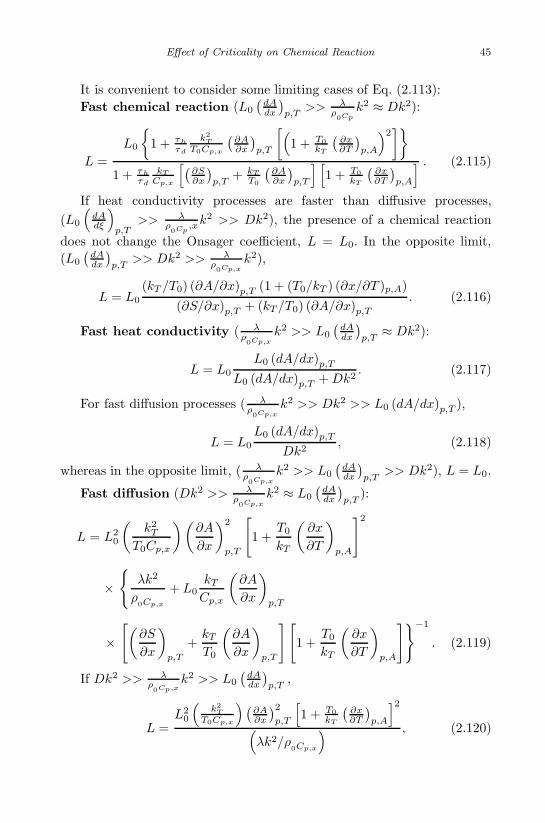
September 11, 2009 10:7 World Scientific Book - 9in x 6in General-nn
Effect of Criticality on Chemical Reaction 45
It is convenient to consider some limiting cases of Eq. (2.113):Fast chemical reaction (L0
(dAdx
)p,T
>> λρ0Cp
k2 ≈ Dk2):
L =L0
{1 + τh
τd
k2T
T0Cp,x
(∂A∂x
)p,T
[(1 + T0
kT
(∂x∂T
)p,A
)2]}
1 + τh
τd
kT
Cp,x
[(∂S∂x
)p,T
+ kT
T0
(∂A∂x
)p,T
] [1 + T0
kT
(∂x∂T
)p,A
] . (2.115)
If heat conductivity processes are faster than diffusive processes,(L0
(dAdξ
)p,T
>> λρ0Cp
,xk2 >> Dk2), the presence of a chemical reaction
does not change the Onsager coefficient, L = L0. In the opposite limit,(L0
(dAdx
)p,T
>> Dk2 >> λρ0Cp,x
k2),
L = L0
(kT /T0) (∂A/∂x)p,T (1 + (T0/kT ) (∂x/∂T )p,A)(∂S/∂x)p,T + (kT /T0) (∂A/∂x)p,T
. (2.116)
Fast heat conductivity ( λρ0Cp,x
k2 >> L0
(dAdx
)p,T≈ Dk2):
L = L0
L0 (dA/dx)p,T
L0 (dA/dx)p,T +Dk2. (2.117)
For fast diffusion processes ( λρ0Cp,x
k2 >> Dk2 >> L0 (dA/dx)p,T ),
L = L0
L0 (dA/dx)p,T
Dk2, (2.118)
whereas in the opposite limit, ( λρ0Cp,x
k2 >> L0
(dAdx
)p,T
>> Dk2), L = L0.
Fast diffusion (Dk2 >> λρ0Cp,x
k2 ≈ L0
(dAdx
)p,T
):
L = L20
(k2
T
T0Cp,x
)(∂A
∂x
)2
p,T
[1 +
T0
kT
(∂x
∂T
)p,A
]2
×{
λk2
ρ0Cp,x
+ L0kT
Cp,x
(∂A
∂x
)p,T
×[(
∂S
∂x
)p,T
+kT
T0
(∂A
∂x
)p,T
][1 +
T0
kT
(∂x
∂T
)p,A
]}−1
. (2.119)
If Dk2 >> λρ0Cp,x
k2 >> L0
(dAdx
)p,T
,
L =L2
0
(k2
T
T0Cp,x
) (∂A∂x
)2p,T
[1 + T0
kT
(∂x∂T
)p,A
]2(λk2/ρ
0Cp,x
) , (2.120)
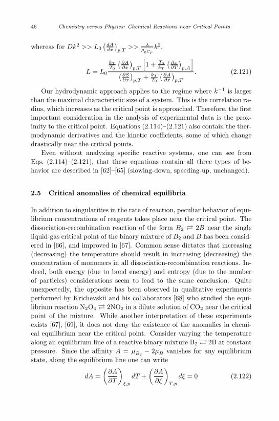
September 11, 2009 10:7 World Scientific Book - 9in x 6in General-nn
46 Chemistry versus Physics: Chemical Reactions near Critical Points
whereas for Dk2 >> L0
(dAdx
)p,T
>> λρ0Cp
k2,
L = L0
kT
T0
(∂A∂x
)p,T
[1 + T0
kT
(∂x∂T
)p,A
](
∂S∂x
)p,T
+ kT
T0
(∂A∂x
)p,T
. (2.121)
Our hydrodynamic approach applies to the regime where k−1 is largerthan the maximal characteristic size of a system. This is the correlation ra-dius, which increases as the critical point is approached. Therefore, the firstimportant consideration in the analysis of experimental data is the prox-imity to the critical point. Equations (2.114)–(2.121) also contain the ther-modynamic derivatives and the kinetic coefficients, some of which changedrastically near the critical points.
Even without analyzing specific reactive systems, one can see fromEqs. (2.114)–(2.121), that these equations contain all three types of be-havior are described in [62]–[65] (slowing-down, speeding-up, unchanged).
2.5 Critical anomalies of chemical equilibria
In addition to singularities in the rate of reaction, peculiar behavior of equi-librium concentrations of reagents takes place near the critical point. Thedissociation-recombination reaction of the form B2 � 2B near the singleliquid-gas critical point of the binary mixture of B2 and B has been consid-ered in [66], and improved in [67]. Common sense dictates that increasing(decreasing) the temperature should result in increasing (decreasing) theconcentration of monomers in all dissociation-recombination reactions. In-deed, both energy (due to bond energy) and entropy (due to the numberof particles) considerations seem to lead to the same conclusion. Quiteunexpectedly, the opposite has been observed in qualitative experimentsperformed by Krichevskii and his collaborators [68] who studied the equi-librium reaction N2O4 � 2NO2 in a dilute solution of CO2 near the criticalpoint of the mixture. While another interpretation of these experimentsexists [67], [69], it does not deny the existence of the anomalies in chemi-cal equilibrium near the critical point. Consider varying the temperaturealong an equilibrium line of a reactive binary mixture B2 � 2B at constantpressure. Since the affinity A = µB2
− 2µB vanishes for any equilibriumstate, along the equilibrium line one can write
dA =(∂A
∂T
)ξ,p
dT +(∂A
∂ξ
)T,p
dξ = 0 (2.122)
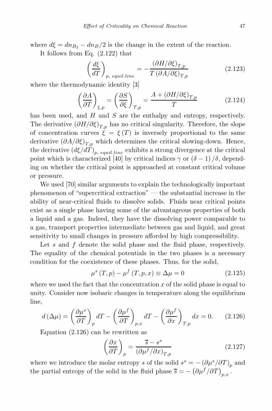
September 11, 2009 10:7 World Scientific Book - 9in x 6in General-nn
Effect of Criticality on Chemical Reaction 47
where dξ = dnB2 − dnB/2 is the change in the extent of the reaction.It follows from Eq. (2.122) that(
dξ
dT
)p, equil.line
= − (∂H/∂ξ)T,p
T (∂A/∂ξ)T,p
(2.123)
where the thermodynamic identity [3](∂A
∂T
)ξ,p
=(∂S
∂ξ
)T,p
=A+ (∂H/∂ξ)T,p
T(2.124)
has been used, and H and S are the enthalpy and entropy, respectively.The derivative (∂H/∂ξ)T,p has no critical singularity. Therefore, the slopeof concentration curves ξ = ξ (T ) is inversely proportional to the samederivative (∂A/∂ξ)T,p which determines the critical slowing-down. Hence,the derivative (dξ/dT )p, equil.line exhibits a strong divergence at the criticalpoint which is characterized [40] by critical indices γ or (δ − 1) /δ, depend-ing on whether the critical point is approached at constant critical volumeor pressure.
We used [70] similar arguments to explain the technologically importantphenomenon of “supercritical extraction” — the substantial increase in theability of near-critical fluids to dissolve solids. Fluids near critical pointsexist as a single phase having some of the advantageous properties of botha liquid and a gas. Indeed, they have the dissolving power comparable toa gas, transport properties intermediate between gas and liquid, and greatsensitivity to small changes in pressure afforded by high compressibility.
Let s and f denote the solid phase and the fluid phase, respectively.The equality of the chemical potentials in the two phases is a necessarycondition for the coexistence of these phases. Thus, for the solid,
µs (T, p)− µf (T, p, x) ≡ ∆µ = 0 (2.125)
where we used the fact that the concentration x of the solid phase is equal tounity. Consider now isobaric changes in temperature along the equilibriumline,
d (∆µ) =(∂µs
∂T
)p
dT −(∂µf
∂T
)p,x
dT −(∂µf
∂x
)T,p
dx = 0. (2.126)
Equation (2.126) can be rewritten as(∂x
∂T
)p
=s− ss
(∂µf/∂x)T,p
(2.127)
where we introduce the molar entropy s of the solid ss = − (∂µs/∂T )p andthe partial entropy of the solid in the fluid phase s = − (∂µf/∂T
)p,x
.
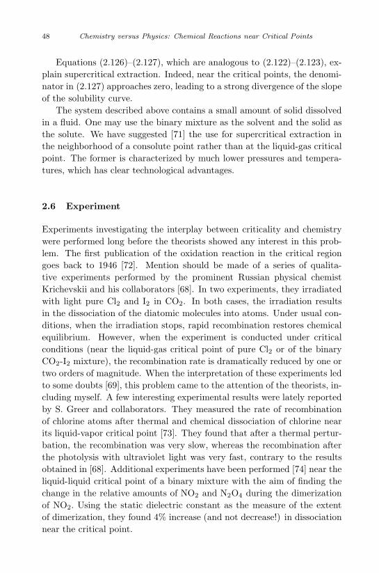
September 11, 2009 10:7 World Scientific Book - 9in x 6in General-nn
48 Chemistry versus Physics: Chemical Reactions near Critical Points
Equations (2.126)–(2.127), which are analogous to (2.122)–(2.123), ex-plain supercritical extraction. Indeed, near the critical points, the denomi-nator in (2.127) approaches zero, leading to a strong divergence of the slopeof the solubility curve.
The system described above contains a small amount of solid dissolvedin a fluid. One may use the binary mixture as the solvent and the solid asthe solute. We have suggested [71] the use for supercritical extraction inthe neighborhood of a consolute point rather than at the liquid-gas criticalpoint. The former is characterized by much lower pressures and tempera-tures, which has clear technological advantages.
2.6 Experiment
Experiments investigating the interplay between criticality and chemistrywere performed long before the theorists showed any interest in this prob-lem. The first publication of the oxidation reaction in the critical regiongoes back to 1946 [72]. Mention should be made of a series of qualita-tive experiments performed by the prominent Russian physical chemistKrichevskii and his collaborators [68]. In two experiments, they irradiatedwith light pure Cl2 and I2 in CO2. In both cases, the irradiation resultsin the dissociation of the diatomic molecules into atoms. Under usual con-ditions, when the irradiation stops, rapid recombination restores chemicalequilibrium. However, when the experiment is conducted under criticalconditions (near the liquid-gas critical point of pure Cl2 or of the binaryCO2-I2 mixture), the recombination rate is dramatically reduced by one ortwo orders of magnitude. When the interpretation of these experiments ledto some doubts [69], this problem came to the attention of the theorists, in-cluding myself. A few interesting experimental results were lately reportedby S. Greer and collaborators. They measured the rate of recombinationof chlorine atoms after thermal and chemical dissociation of chlorine nearits liquid-vapor critical point [73]. They found that after a thermal pertur-bation, the recombination was very slow, whereas the recombination afterthe photolysis with ultraviolet light was very fast, contrary to the resultsobtained in [68]. Additional experiments have been performed [74] near theliquid-liquid critical point of a binary mixture with the aim of finding thechange in the relative amounts of NO2 and N2O4 during the dimerizationof NO2. Using the static dielectric constant as the measure of the extentof dimerization, they found 4% increase (and not decrease!) in dissociationnear the critical point.
September 11, 2009 10:7 World Scientific Book - 9in x 6in General-nn
Effect of Criticality on Chemical Reaction 49
A review of early development in this field can be found in [75]. Specialattention should be paid to the Snyder and Eckert article: “Chemical kinet-ics at a critical point” [76], where, in contrast to the well-known “slowing-down”, they found “speeding-up” (increase by some 40%) of the reactionrate of the isoprene with maleic anhydride in the vicinity of the upper crit-ical solution point of two liquid-liquid mixtures (hexane-nitrobenzene andhexane-nitroethane). This result was obtained more than twenty years be-fore the theoretical idea of the “piston effect”, and authors proposed anexplanation related to the dilute solution of the reactants.
Extensive studies of the rate of chemical reactions in the vicinity of thecritical point were carry out by J. K. Baird and collaborators. In their 1998article [62], they described the measurement of the rate of five hydrolysisfirst-order reactions near the consolute point of three binary mixtures (tert-amyl chloride and tert-butyl chloride in isobutyric acid-water, 3-chloro-3-methylpentane and 4-methylbenzyl bromide in 2-butoxyethanol-water, tert-butyl bromide in triethylamine-water). All these reactions produce a strongelectrolyte, and the progress of the reaction was followed by measuringthe conductance in the vicinity of the lower and upper critical consolutepoints. All measurements showed a slowing-down effect within a few tenthsof a degree on either side of the consolute temperature, in agreement withprevious experiments. The measurement of 2-chloro-2-methylbutane nearthe critical point of the mixture isobutyric acid-water, has been repeated[63]. The more careful, later experiment (system was well-stirred in the two-phase region, and account was taken of the small shift ∆Tc = 0.2 K of thecritical temperature of the solvent due to the presence of the reactant) yieldsdifferent results. Above TC , the rate of reaction showed slowing-down,while below TC , in the two-phase region, the rate of reaction increasedupon approaching the critical point (“speeding-up” predicted by the “pistoneffect”). To check whether the speeding-up of the reaction rate is connectedwith the coexistence of two immiscible phases, the experiment was carriedout on 2-bromo-2-methylpropane in triethylamine-water, analogous to thatperformed in [63]. In contrast to isobutyric acid-water used in [63], thelatter mixture has a lower critical solution temperature. In spite of thisdifference, the results of the experiments were the same: slowing-downabove the critical temperature and speeding-up below, which means thatthe “speeding-up” effect is associated with the critical point and not withthe number of phases in the system.
Another improvement over the original experiments was that visual de-tection of critical opalescence to determine the critical temperature was
September 11, 2009 10:7 World Scientific Book - 9in x 6in General-nn
50 Chemistry versus Physics: Chemical Reactions near Critical Points
replaced by the association of the critical temperature with the tempera-ture of the onset of the sharp change in electrical conductivity when criticalopalescence occurs [64]. The authors measured the rate of the Menschutkinreaction between benzyl bromide and triethylamine near the consolute pointof triethylamine-water, which can be compared with the old measurements[76] of the Menshutkin reaction on ethyl iodide. For temperatures below TC ,
they could clearly see the critical slowing-down of the reaction rate show-ing the weak singularity, while above TC , a few measured points closest toTC gave a hint of speeding-up. These results agree with those obtainedearlier [76].
The next question investigated concerned the generality of the effectfound. In particular, does the effect exist for other types of reactions, say,of second-order, and not of first-order kinetics? To answer this question, theexperiment was performed [65] with the saponification of ethyl acetate bysodium hydroxide near the consolute point of the 2-butoxyethanol-water,which is known to exhibit [77] second-order kinetics. The experiment [65]shows slowing-down for temperatures below TC . For T > TC , the results ofthe experiment are not clear: one cannot a rule out speeding-up, but onlyfuture experiments will definitively answer this question.
An important comment has been emphasized in [62], [63] regarding thequantitative description of the slowing-down and speeding-up of the reac-tion rate. The rate of reaction is proportional to thermodynamic deriva-tive of the Gibbs free energy difference ∆G separating products from re-actance with respect to the extent of reaction ξ. As described in section2.1, the singularity x of this quantity, (∂∆G/∂ξ)a,b,... ∼ |(T − TC) /TC |x,at the critical point depends on number of fixed “density type” variablesa, b (entropy, volume, concentrations of the chemical components, extentof reaction). Namely, if one density is fixed, then one finds a “weak” sin-gularity (x = 0.11 or x = 0.33, depending on the thermodynamical pathapproaching the critical point — fixed pressure or temperature or along thecoexistence curve). For densities not held fixed, the singularity is “strong”(x = 1.24 or x = 4.9). Finally, for two or more fixed densities, x = 0 andthere is no singularity of the reaction rate at the critical point. In turn, thenumber of fixed densities, i.e., those which do not participate in at leastone chemical reaction, depends on the number of reactions occurring in thesystem. Estimating the number of reactions is not trivial, as seen fromthe following example [63]. One of the components of a solvent (isobutyricacid), which does not participate in the hydrolysis reaction, might never-theless react with the alcohols present in the system, thereby changing the
September 11, 2009 10:7 World Scientific Book - 9in x 6in General-nn
Effect of Criticality on Chemical Reaction 51
behavior of the reaction rate by changing the number of reactions and thenumber of densities held fixed.
In addition to conductance measurements, the same experimental groupused another method to analyzing the progress of a chemical reaction [78],namely, the measurement of the rate of appearance of a phase that is notcompletely miscible with a liquid mixture, such as the gas phase. Threereactions have been studied: 1) acetone dicarboxylic acid in aniline cat-alyzed decomposition of acetone dicarboxylic acid in isobutyric acid-water,2) benzene diazonium tetrafluoroborate in the decomposition of benzene di-azonium tetrafluoroborate in 2-butoxyethanol-water, 3) ethyl diazoacetatein the acid catalyzed decomposition of ethyl diazoacetate in isobutyric acid-water. In all cases, the critical point did not effect the rates of the reactions.
September 11, 2009 10:7 World Scientific Book - 9in x 6in General-nn
Chapter 3
Effect of Chemistry on CriticalPhenomena
3.1 Change of critical parameters due to a chemicalreaction
Chemical reactions near the critical points are routinely studied near theconsolute points of a binary mixture which plays the role of a solvent. Thepresence of a reactant, as well as impurities, pressure or electric field changesthe critical parameters of a binary mixture. There is only limited knowl-edge of the relationship between the shifts of the critical parameters whenthe perturbation is applied. For example, it is known [3] that an impuritywill cause a critical temperature shift equal to that of the critical compo-sition only when the solubilities in the two components are roughly equal.However, it was found that two different impurities (water [79] and acetone[80]), which have quite different solubilities in the two components of themethanol-cyclohexane mixture, induce equal relative shifts in critical tem-perature and composition, ∆TC/TC,0 = ∆xC/xC,0. The same relation hasbeen observed [81] in a wide range of systems (Fig. 3.1). These data havebeen obtained by isobaric measurements upon the addition of impurities.
There are different experimental ways of finding the critical parametersTC and pC of a system. The simplest, but less precise method is basedon visual detection of critical opalescence to determine the critical temper-ature. For ionic conductors, the critical temperature is identified by thesharp change in electrical conductivity [64]. Alternatively, one can use thedilatometric method of measuring the height of the liquid in the capillaryside-arm as a function of temperature. A change in the slope of this curveoccurs at the critical temperature [62]. Another method is the acoustictechnique, using the fact that the velocity of sound reaches a minimum atthe critical point [82]. Experiments show that the critical temperature TC
53
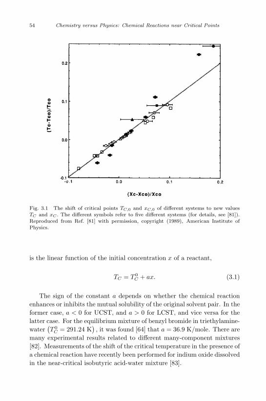
September 14, 2009 16:35 World Scientific Book - 9in x 6in General-nn
54 Chemistry versus Physics: Chemical Reactions near Critical Points
Fig. 3.1 The shift of critical points TC,0 and xC,0 of different systems to new valuesTC and xC . The different symbols refer to five different systems (for details, see [81]).Reproduced from Ref. [81] with permission, copyright (1989), American Institute ofPhysics.
is the linear function of the initial concentration x of a reactant,
TC = T 0C + ax. (3.1)
The sign of the constant a depends on whether the chemical reactionenhances or inhibits the mutual solubility of the original solvent pair. In theformer case, a < 0 for UCST, and a > 0 for LCST, and vice versa for thelatter case. For the equilibrium mixture of benzyl bromide in triethylamine-water
(T 0
C = 291.24 K), it was found [64] that a = 36.9 K/mole. There are
many experimental results related to different many-component mixtures[82]. Measurements of the shift of the critical temperature in the presence ofa chemical reaction have recently been performed for indium oxide dissolvedin the near-critical isobutyric acid-water mixture [83].
September 11, 2009 10:7 World Scientific Book - 9in x 6in General-nn
Effect of Chemistry on Critical Phenomena 55
3.2 Modification of the critical indices
In this section, we describe the changes in critical phenomena arising fromthe presence of chemical reactions. The singularities of the thermodynamicand kinetic quantities near the critical points are determined by the criticalindices. The calculations of these indices assumes the constancy of someintensive variables, say, pressure p or chemical potentials µ, whereas inpractice it is impossible, for example, to ensure the constancy of µ (one hasto vary the concentrations during the course of the experiment). Similarly,p remains practically unchanged near the liquid-liquid critical point sincethe experiment is carried out in the presence of saturated vapor. On theother hand, it is quite difficult to ensure the constancy of p near the liquid-gas critical point where a fluid is highly compressible.
In order to compare theoretical calculations for an ideal one-componentsystem with experimental data obtained for “real” systems, Fisher [84] de-veloped the theory of renormalization of critical indices. The main idea ofrenormalization can be explained by the following simple argument. Fora pure substance, mechanical stability is determined by (∂p/∂v)T < 0.The condition for diffusion stability in a binary mixture has the form(∂µ/∂x)T,p > 0, which, by a simple thermodynamic transformation, canbe rewritten as (∂p/∂v)T,µ < 0. Therefore, at constant chemical poten-tial µ, the critical behavior of a binary mixture, which is defined by thestability conditions, will be the same as that of a pure substance. Mul-ticomponent systems behave in an analogous manner, namely, the stabil-ity condition for a n-component mixture is determined by the condition(∂p/∂v)T,µ1...µn−1
< 0, where n− 1 chemical potentials are held constant.However, the critical parameters now depend on the variables µi, and inorder to obtain experimentally observable quantities which correspond toconstant concentration x, one has to pass from T (µ) to T (x). As a result,when one goes from a pure substance to a binary mixture, the critical indicesabove and below a critical point are multiplied by ± (1− α)−1 [84], whereα is the critical index of the specific heat at constant volume. The minussign refers to the specific heat at constant volume and the plus sign refersto all other critical indices. We have discussed [85] the renormalization ofthe critical indices associated with the presence of chemical reactions. Asan example, let us again consider a binary fluid mixture A1 −A2 with thesingle reaction ν1A1 + ν2A2 = 0 (say, the isomerization reaction). Thisequation means that the law of mass action is satisfied, i.e., one gets forthe extent of reaction A = ν1µ1 + ν2µ2 = 0, which, in turn, reduces by
September 11, 2009 10:7 World Scientific Book - 9in x 6in General-nn
56 Chemistry versus Physics: Chemical Reactions near Critical Points
one the number of thermodynamic degrees of freedom in a binary mixture.Therefore, the reactive binary system has an isolated critical point, and thecritical indices of this system are the same as those of a pure fluid,(
∂υ
∂p
)T,A=0
∼ Cp,A=0 ∼(T − TC
TC
)−γ
;
(∂v
∂p
)s,A=0
∼ Cv,A=0 ∼(T − TC
TC
)−α
, etc.
(3.2)
where υ = 1/ρ is the specific volume.It is interesting to compare (3.2) with the case of a frozen chemical
reaction (no catalyst added). The system considered is then a binary mix-ture with a liquid-gas critical line. The renormalized critical indices of suchsystems are well known [84]
Cp,ξ ∼(∂υ
∂p
)T,ξ
∼(
T−TC
TC
)−α/(1−α).
;
Cv,ξ ∼(∂υ
∂p
)s,ξ
∼(
T−TC
TC
)α/(1−α)
.
(3.3)
The correspondence between (3.2) and (3.3) becomes obvious from thethermodynamic relation [3]
Cp,A=0 = Cp,ξ − h2 (∂ξ/∂A)T,p (3.4)
where h is the heat of reaction. In fact, the asymptotic behavior of theleft-hand side of Eq. (3.4) on approaching a critical point is determined bythe second term on the right-hand side rather than by the first term, whichhas a weaker singularity.
The occurrence of a chemical reaction in the system under considerationmodifies the critical indices of the observable specific heats at constantvolume and constant pressure (or inverse velocity of sound) compared to asystem with a frozen chemical reaction. They are changed from α/ (1− α)and −α/ (1− α) to −α and −γ, respectively. For example, the specificheat at constant volume has a weak singularity at the critical point whena chemical reaction occurs, but a finite, cusped behavior in the absence ofa chemical reaction.
The singularities become weaker for many-component mixtures. A com-mon situation is that the solutes undergo various chemical transformationswhile the solvent does not. As an example, consider the critical systemcontaining a reactive binary mixture dissolved in some solvent. Due to theexistence of a neutral third component, the system has a line of critical
September 11, 2009 10:7 World Scientific Book - 9in x 6in General-nn
Effect of Chemistry on Critical Phenomena 57
points rather than an isolated critical point, as is the case for a reactivebinary mixture.
Let us consider the frozen chemical reaction. The singularities of thethermodynamic quantities in a ternary mixture at constant chemical po-tential µ0 of the solvent are similar to those of a binary mixture. Theliquid-liquid critical points depend only slightly on the pressure, so thatthe parameter RρC (dTC/dp) (ρC is the critical density) is very small. Thisparameter determines the region of renormalization [86]. Therefore, renor-malization is absent, as in the vicinity of the λ line in helium, and
Cp,ξ,µ0∼ Cυ,ξ,µ0
∼ φ (µ0)−α ; φ (µ0) ≡
T − TC (µ0)TC (µ0)
. (3.5)
However, measurements are taken at constant number of solvent particlesrather than at µ0 = const. According to renormalization, near the liquid-liquid critical points, one obtains
Cp,ξ,N0 ∼ Cυ,ξ,N0 ∼(T − TC
TC
)α/(1−α)
. (3.6)
Unlike the liquid-liquid critical point, there are two renormalizationsin the vicinity of liquid-gas critical point; the first occurs when passingfrom the binary to the ternary mixture, and the second renormalizationtakes place when passing from µ0 = const to N0 = const. In the region ofrenormalization of the ternary mixture, one gets
Cp,ξ,µ0∼ φ−α/(1−α); Cυ,ξ,µ0
∼ φα/(1−α) (3.7)
and for N0 = const,
Cp,ξ,N0 ∼ φα/(1−α); Cυ,ξ,N0 ∼ const. (3.8)
Comparing (3.6) and (3.8), one concludes that without a chemical reac-tion, cusp-like behavior exists for both specific heats near the liquid-liquidcritical points, but only for the specific heat at constant pressure near theliquid-gas critical points.
When a chemical reaction takes place, the singularities near the criticalpoints can be found from the thermodynamic relations, analogous to (3.4),
Cp,N0,A=0 = Cp,N0,ξ − T (∂ξ/∂A)T,p,N0(∂A/∂T )2p,N0,ξ
Cυ,N0,A=0 = Cυ,N0,ξ − T (∂ξ/∂A)υ,T,N0(∂A/∂T )2v,N0,ξ .
(3.9)
For both types of critical points, the singularities of thermodynamicquantities in a system undergoing a chemical reaction (A = 0) are deter-mined by the second term on the right-hand sides of Eqs. (3.9). The factor
September 11, 2009 10:7 World Scientific Book - 9in x 6in General-nn
58 Chemistry versus Physics: Chemical Reactions near Critical Points
∂A/∂T in the latter terms remains finite at the critical point, whereas thesecond factor has the following asymptotic behavior,
(∂ξ/∂A)T,p,µ0∼ φ−γ ; (∂ξ/∂A)υ,T,µ0
∼ φ−α (3.10)
and, after renormalization,
(∂ξ/∂A)T,p,N0∼(T − TC
TC
)− α/(1−α)
;
(∂ξ/∂A)υ,T,N0∼(T − TC
TC
)α/(1−α)
.
(3.11)
Therefore, for a system undergoing a chemical reaction, one obtains from(3.9) and (3.11),
Cp,N0,A=0 ∼(∂υ
∂p
)T,N0,A=0
∼ φ−α/(1−α);
Cυ,N0,A=0 ∼(∂υ
∂p
)v,N0,A=0
∼ φα/(1−α).
(3.12)
Comparing (3.6) and (3.8) with (3.12) yields that the existence of achemical reaction leads to a magnification of the singularities of the specificheats at constant pressure for both types of critical points, from cusp-likebehavior α/ (1− α) to a weak singularity −α/ (1− α). On the other hand,the specific heat at constant volume changes its asymptotic behavior fromconstant to cusp-like only near the liquid-gas critical point. In principle, onecan detect such a magnification experimentally. Experiments are slightlyeasier to perform near the liquid-liquid critical points, because these pointsusually occur at atmospheric pressure and room temperature.
Consider now the singularities of the dielectric constant ε and electri-cal conductivity σ at the critical point of reactive systems. These quan-tities can be obtained by choosing poorly conducting liquid mixtures fordielectric measurements and strongly conducting mixtures for conductivitymeasurements. One can also measure ε and σ simultaneously placing thefluid between two parallel plates or coaxial cylindrical electrodes with analternative current bridge. The fluid then acts in the bridge circuit as afrequency-dependent impedance with balanced capacity and resistive com-ponents [87]. Near the critical points, large fluctuations affect all ther-modynamic and kinetic properties including those which are characterizedby σ and ε. There are hundreds of experimental papers, of which we willdescribe only a few. Of special importance are chemical reactions in eco-logical clean near-critical water. At high temperature and pressure, water
September 11, 2009 10:7 World Scientific Book - 9in x 6in General-nn
Effect of Chemistry on Critical Phenomena 59
becomes self-ionized with a high conductivity, resembling molten salts [88].The special case is the dissociation of a weak acid in water near an acid-water liquid-liquid critical point,
HA+H2O � A−+H3O+. (3.13)Measurements of the conductivity as a function of temperature have
been performed near the liquid-liquid critical points for the systems isobu-tyric acid-water [89], [90] and phenol-water [90]. Different explanationshave been proposed for the anomaly in the conductivity near the criticalpoint [91]: 1) The anomaly is due to viscous drag of the acid anion [89]and, hence, according to the Stokes law, it is proportional to the inverseof the viscosity η, σ ∼ η−1 = τνzη = τ0.031, where τ = (T − TC) /TC , andν = 0.63, zη = 0.05 are the critical indices for the correlation length andviscosity, respectively; 2) The anomaly of σ is related to the anomaly in theproton-transfer rate [92], which, in turn [93], has the temperature depen-dence of the nearest-neighbor correlation function, σ ∼ τ1−α = τ0.89, whereα = 0.11 is the critical index for the heat capacity at constant pressureand composition; 3) A percolation model for conductivity leads [90] to ananomaly of the form σ ∼ τ2β = τ0.65, where β = 0.325 is the critical indexdescribing the coexistence curve; 4) The anomaly of σ is related to that ofthe extent of the acid dissociation [94], which leads [95] to σ ∼ τ1−α = τ0.89.
A detailed analysis of the experimental data obtained in [89], [90] hasbeen carried out [96], taking account of the background contribution dueto the normal temperature dependence of the dissociation constant anddue to the confluent critical singularity. The leading critical anomaly ofthe conductance was found to be characterized by a critical index 1 − α,consistent with its connection with an anomaly in the extent of the disso-ciation reaction and also for an anomaly in the proton-transfer rate.
The static dielectric constant for the dimerization reaction2NO2 � N2O4 has been measured [74] in a solvent mixture ofperfluoromethylcyclohexane-carbon tetrachloride near the liquid-liquid crit-ical point of the solvent. The appropriate choice of reaction (no dipolemoment for the N2O4 molecule, and a small moment for NO2) and of thesolvent (the components of low polarity make the “background” dipole mo-ment very small) assure the high precision of measurements. The dielectricconstant was found to have a 1−α anomaly near the critical point, the sameas the conductivity. For a mixture of polystyrene and diethyl malonate nearthe liquid-liquid critical point in the absence of chemical reactions, the di-electric constant was measured [97] as a function of frequency in the range20 KHz to 1 MHz. No anomaly was found in the dielectric relaxation time.
September 11, 2009 10:7 World Scientific Book - 9in x 6in General-nn
60 Chemistry versus Physics: Chemical Reactions near Critical Points
3.3 Singularity in the degree of dissociation near acritical point
At the end of the previous section, we considered the anomalies in elec-troconductivity near the critical point, which are caused by the scatteringof charged ions by strongly enhanced concentration fluctuations. However,apart from the anomalies of scattering processes, an additional factor hasto be taken into account, namely, the density of ions may have a singularitynear the critical point due to the chemical reaction [94]. Assume that thedissociation reaction
CD � C++D− (3.14)
occurs between the solutes CD, C+ and D− near the critical point of thesolvent E. The condition for chemical equilibrium has the following form,
A ≡ µCD − µC+ − µD− = 0. (3.15)
The constraint of electroneutrality
NC+ = ND− , (3.16)
permits one to write the differential of the Gibbs free energy in the form
dG = −SdT + V dp+ µEdNE + µCDdNCD − (µC+ + µD−) dNC+ . (3.17)
It is convenient [95] to express the thermodynamics in terms of the totalnumber N1 of moles of CD, both dissociated and undissociated, and of totalnumber N2 of moles of CD and E,
N1 = NCD +NC+ ; N2 = N1 +NE. (3.18)
It is also convenient to define intensive variables,
ξ =NC+
N2; χ =
N1
N2; g =
G
N2; υ =
V
N2; s =
S
N2. (3.19)
Using Eqs. (3.15)–(3.19), one may rewrite Eq. (3.17),
dg = −sdT + υdp−Adξ + (µCD − µE) dχ. (3.20)
Note that for a closed system, the variable χ remains constant, indepen-dent of the extent of reaction ξ. Usually the temperature changes during theexperiment while the pressure remains constant. The extent of reaction,i.e., the number of charges, is defined by the derivative (∂ξ/∂T )p,χ,A=0 .
This derivative is taken under the condition that two extensive (“field”)variables, p and A, and one intensive (“density”) variable χ are kept fixed.
September 11, 2009 10:7 World Scientific Book - 9in x 6in General-nn
Effect of Chemistry on Critical Phenomena 61
According to the general theory [38], this derivative has only a “weak”singularity at the critical point, defined by the critical index α = 0.12,(
∂ξ
∂T
)p,χ,A=0
≈(T − TC
TC
)−α
. (3.21)
Thus far, we have considered a one-phase system. Let us now considera ternary mixture (components 1, 2 and 3) existing in two phases, whichwe label α and β. The chemical reaction allowed is of the form 1 � 2 + 3.For example, this model describes a one-component system (say HI) nearits liquid-gas critical point (TC = 150 K for HI) dissociated into two species(2HI � H2+I2). The question is: How will the concentration of the reagentsvary near the critical point of a three-component system? For a smallequilibrium constant of reaction, we may neglect the small shift from thecritical point of a one-component system.
Denoting by µαi and µβ
i the chemical potentials of the i-th componentin each phase, one gets for the equilibrium state,
µα1 = µβ
1 ; µα2 = µβ
2 ; µα3 = µβ
3 . (3.22)
The condition of chemical equilibrium, similar to Eq. (3.15), has the form
µα1 − µα
2 − µα3 = 0. (3.23)
A similar condition in the second phase follows from (3.22), but does notproduce any additional restriction.
We are interested in equilibrium properties. Therefore, the thermody-namic path we choose is a displacement along the equilibrium line, keepingthe pressure constant,
d(µα
1 − µβ1
)= d
(µα
2 − µβ2
)= d
(µα
3 − µβ3
)= d (µα
1 − µα2 − µα
3 ) = 0. (3.24)
Choosing as independent variables the mole fractions of the first andthe second component in each phase, xα
1 , xα2 , x
β1 , x
β2 , and the temperature
T, one can rewrite Eqs. (3.24) in the following forms
µα11dx
α1 + µα
12dxα2 − µβ
11dxβ1 − µβ
12dxβ2 =
(µβ
1T − µα1T
)dT,
µα21dx
α1 + µα
22dxα2 − µβ
21dxβ1 − µβ
22dxβ2 =
(µβ
2T − µα2T
)dT,
µα31∂xdx
α1 + µα
32dxα2 − µβ
31dxβ1 − µβ
32dxβ2 =
(µβ
3T − µα3T
)dT,
(µα11 − µα
21 − µα31) dx
α1 + (µα
12 − µα22 − µα
32) dxα2 = − (µα
1T − µα2T − µα
3T ) dT
(3.25)
September 11, 2009 10:7 World Scientific Book - 9in x 6in General-nn
62 Chemistry versus Physics: Chemical Reactions near Critical Points
where (∂µα,β
i
∂xα,βj
)p,T,xi �=xj
≡ µα,βi,j ;
(∂µα,β
i
∂T
)p,xj
≡ µα,βi,T . (3.26)
Solutions of Eqs. (3.25) for dxα,βi /dT are(
dxα,βi
dT
)p,equil.
=∆α,β
i
∆(3.27)
where the subscript equil refers to the equilibrium line, ∆ is the 4 × 4determinant of Eqs. (3.25), and ∆α,β
i is the determinant with one of therows replaced by the row of coefficients from the right-hand side of Eqs.(3.25). Simple analysis shows [94] that ∆ has no singularities at the critical
point, whereas ∆α,βi is proportional to the factor µα,β
11 µα,β22 −
(µα,β
2
)2
which
can be rewritten as(∂µα,β
12 /∂x)
p,T,µ1(p,T,x1). The line of critical points is
thus determined by the vanishing of the next derivative of µα,β2 with respect
to x [3], which, having one “density” variable fixed, has a weak singularity(3.21) at the critical point. Then, the x-T curves have an infinite slope atthe critical points.
The coincidence of the final results for the two cases results from theelectroneutrality of the four-component mixture which makes it isomorphicto the three-component mixture. If the four-component mixture is com-prised of two phases, each phase can be described by two mole fractions,say x1 and x2, while x3 = x4 = (1− x1 − x2) /2. Therefore, the equilibriumequations will have the same form, Eq. (3.25), resulting in Eq. (3.21).
3.4 Isotope exchange reaction in near-critical systems
The results of experiments performed on isobutyric acid (CO2H) - deu-terium oxide (D2O) binary mixture are an example of the shift of criticalparameters and the modification of critical indices due to a chemical reac-tion. Peculiar to this system is the capability of the proton of the carboxylgroup of isobutyric acid to exchange with the deuteron of deuterium oxide(isotope exchange reaction). This reaction produces more than two species,and the concentrations of CO2H and D2O are not the same because of theisotope exchange reaction. The experiments include the visual observationof the phase separation and light scattering [98]. The results have beencompared with those for isobutyric acid-water (CO2H/H2O) and deuter-ated isobutyric acid-deuterium oxide (CO2D/D2O) systems. Appreciable
September 11, 2009 10:7 World Scientific Book - 9in x 6in General-nn
Effect of Chemistry on Critical Phenomena 63
amounts of additional species due to isotope exchange distort the coexis-tence curve, shifting the critical solution concentration xC away from theconcentration x0 where the maximum phase separation temperature Tmax
occurs. This makes the critical indices γ and ν of the correlation length
(ξ = ξ0
(T−TC
TC
)−γ
) and isothermal compressibility (k = k0
(T−TC
TC
)−ν
)in the one-phase region (T > TC) different from those of the coexistingtwo-phase region (T < TC). It was found that xC (mass fraction of isobu-tyric acid) equals 0.358 at TC = 44.90◦C, which differs from x0 = 0.310and Tmax = 45.11◦C. In the one-phase region, γ = 1.25, ν = 0.63 andξ0 = 3.13 A in agreement with the renormalization group results, whereasin the coexistence two-phase region, the critical indices appear to be renor-malized with γ = 1.39, ν = 0.76 and ξ0 = 0.6 A. As result of exchangeequilibria, CO2H/D2 O is effectively a three-component system in the co-existence two-phase region [98], and the renormalized critical indices arein agreement with those near the plait point of a ternary liquid mixtureethanol-water-chloroform [99]. An alternative explanation of these experi-ments is given in [100], [101].
3.5 Singularities of transport coefficients in reactivesystems
In order to determine the influence of a chemical reaction on the transportcoefficients, one can use the same mode-mode coupling analysis [102] usedin the previous chapter for finding the influence of criticality on the rate ofa chemical reaction. That is, one calculates the correlation functions which,in turn, define the change of the transport coefficients. A different way ofattacking this problem is by dynamic renormalization group methods [103],which we will briefly describe in the next section.
3.5.1 Mode-coupling analysis
Just as for the reaction rates, the transport coefficients (shear viscosity ηand diffusion coefficient D) can be written as time integrals of the correla-tions of appropriate fluxes, which, in turn, can be expanded in powers of thehydrodynamic variables. In calculating the critical corrections ∆η and ∆D,one neglects the small critical indices, thus assuming the Ornstein-Zernikeform for the susceptibility. The most significant contribution to ∆η is the
September 11, 2009 10:7 World Scientific Book - 9in x 6in General-nn
64 Chemistry versus Physics: Chemical Reactions near Critical Points
integral over wavenumber k of the form [36]
∆η ∼∫ k2
k1
dk
k + L. (3.28)
The upper limit k2 is related to an unimportant cutoff, and the lower limitk1, the inverse correlation length ξ−1, vanishes at the critical point. Whenthere is no reaction (Onsager coefficient L = 0), this integral diverges log-arithmically at the critical point. A more careful calculation of ∆η leadsto a weak power divergence rather than a logarithmic divergence. How-ever, when L �= 0, the integral (3.28) does not diverge. It follows that theviscosity in reactive systems remains finite at the critical point. Note thatif L is extremely small (extremely slow chemical reaction), then η growsupon approaching the critical point, but its growth is terminated when thecorrelation length becomes of order L−1.
The calculation of the mode-coupling corrections to the wavenum-ber (frequency)-dependent diffusion coefficient in reactive binary mixtures[102], [36] yields
∆D =κBT
6πρξX2η
[K (X)− βX3
Y 3K (Y )
](3.29)
where ξ is the correlation length, X = kξ, Y = X√δ/ (1 +X + δ), δ =
L/η, β = δ/ (1 + δ). The function K (X) is given by
K (X) =34[1 +X2 +
(X3 −X−1
)tan−1X
]. (3.30)
When L = 0, one regains the well-known result for non-reactive mixtures[102]. The influence of the chemical reaction on the diffusion coefficientcan easily be seen in the two limiting cases of low frequencies kξ < 1 (the“hydrodynamic” region) and high frequencies kξ > 1 (the “critical” region).
a) For kξ < 1, K (X) ∼ X2, and
∆D =κBT
6πρξη
(1− β1/2
). (3.31)
The usual result [102] η∆D ∼ ξ−1 is obtained, but with a renormalizedcoefficient. Because D = α (∂A/∂ξ)T,p , and since η is not divergent inreactive systems, α diverges like ξ.
b) For kξ > 1, K (X) ∼ (3π/8)X2, and
∆D =κBT k
16ρ (η + L). (3.32)
This result is similar to that obtained for a nonreactive binary mix-ture, except for the renormalization of the coefficient of k. Therefore, thediffusion coefficient in reactive systems still vanishes like ξ−1 but with amodified coefficient of proportionality due to the chemical reaction.
September 11, 2009 10:7 World Scientific Book - 9in x 6in General-nn
Effect of Chemistry on Critical Phenomena 65
3.5.2 Renormalization group methods
The hydrodynamic equations (2.61)–(2.64) are written for local space-averaged variables. The renormalization group technique allows one toaverage over increasingly large regions, thereby reducing the number ofeffective degrees of freedom of the system. Due to the divergence of thecorrelation length, such a procedure is of special importance near the crit-ical points, where the increasing number of degrees of freedom becomesimportant. Efficient computer programs have been developed for study-ing static critical phenomena [104], and they have been extended to coverdynamic critical phenomena as well [103].
The starting point is the identification of slow modes, whose relaxationtimes approach zero at small wavenumbers, and also (if the order parameteris not conserved) the order-parameter mode. Therefore, one has to assigneach system to the appropriate model A − H [103]. Such an identifica-tion also depends on the regimes of wavenumber which define the relativeimportance of the different modes.
The distinctive feature of reactive systems is the existence of a ho-mogeneous chemical mode, which converts the concentration into a non-conserved parameter. Milner and Martin [40] performed a renormalizationgroup analysis for a reactive binary mixture, improving the result of thelinear analysis of the critical slowing-down described in Sec. 2.1.
They found [40] that the critical slowing-down of a chemical reactionoccurs for kH < k < kC , where kC and kH are the inverse length scalesfor diffusion and heat conductivity. The slowing-down is governed by thestrong critical index γ+α+ ην 1.37 rather than by γ ≈ 1.26 obtained inthe linear theory.
September 11, 2009 10:7 World Scientific Book - 9in x 6in General-nn
Chapter 4
Phase Separation in Reactive Systems
4.1 Multiple solutions of the law of mass action
Thus far, we have considered single-phase reactive systems near their criti-cal point. Another interesting problem is phase separation in reactive sys-tems as compared to non-reactive systems. Will the presence of a chemicalreaction, induced, say, by a very small amount of catalyst, stimulate or re-strict the process of phase separation? In this chapter we will consider theseproblems, but we first have to consider the possibility of multiple solutionsof the law of mass action. Two (or more) coexisting phases which have thesame temperature and pressure are different in concentrations of differentcomponents and, therefore, in conducting chemical reactions. This meansthat the law of mass action has more than one solution for the concentrationat given temperature and pressure.
Let us clarify the possibility of multiple solutions of the law of massaction. The chemical potential of the i-th component can be written in thefollowing form
µi = µ0i (p, T ) + κBT ln (γi, xi) (4.1)
where the activity γi determines the deviation from the ideal system, forwhich γi = 1. Using (4.1), one can rewrite the law of mass action as
xν11 , xν2
2 , . . . , xνnn = Kid. (p, T ) γ−ν1
1 , γ−ν22 , . . . , γ−νn
n ≡ K. (4.2)
The chemical equilibrium constant for the ideal system Kid is deter-mined by the functions µ0
i in (4.1), i.e., by the properties of individualnon-reactive components, whereas for non-ideal systems, K also dependson the interactions among the components. For ideal systems, all γi = 1,and Eq. (4.2) has a single set of solutions x1, x2, . . . , xn. This was provedmany years ago [105] for isothermal-isochoric systems. Another proof was
67
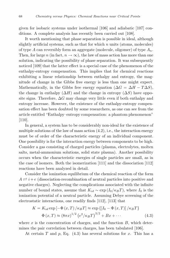
September 11, 2009 10:7 World Scientific Book - 9in x 6in General-nn
68 Chemistry versus Physics: Chemical Reactions near Critical Points
given for isobaric systems under isothermal [106] and adiabatic [107] con-ditions. A complete analysis has recently been carried out [108].
It worth mentioning that phase separation is possible in ideal, althoughslightly artificial systems, such as that for which n units (atoms, molecules)of type A can reversibly form an aggregate (molecule, oligomer) of type An.Then, for large n (in fact, n→∞), the law of mass action has more than onesolution, indicating the possibility of phase separation. It was subsequentlynoticed [109] that the latter effect is a special case of the phenomenon of theenthalpy-entropy compensation. This implies that for chemical reactionsexhibiting a linear relationship between enthalpy and entropy, the mag-nitude of change in the Gibbs free energy is less than one might expect.Mathematically, in the Gibbs free energy equation (∆G = ∆H − T∆S),the change in enthalpy (∆H) and the change in entropy (∆S) have oppo-site signs. Therefore, ∆G may change very little even if both enthalpy andentropy increase. However, the existence of the enthalpy-entropy compen-sation effect has been doubted by some researchers, as one can see from thearticle entitled “Enthalpy–entropy compensation: a phantom phenomenon”[110].
In general, a system has to be considerably non-ideal for the existence ofmultiple solutions of the law of mass action (4.2), i.e., the interaction energymust be of order of the characteristic energy of an individual component.One possibility is for the interaction energy between components to be high.Consider a gas consisting of charged particles (plasma, electrolytes, moltensalts, metal-ammonium solutions, solid state plasma). Another possibilityoccurs when the characteristic energies of single particles are small, as inthe case of isomers. Both the isomerization [111] and the dissociation [112]reactions have been analyzed in detail.
Consider the ionization equilibrium of the chemical reaction of the formA � i+ e (dissociation-recombination of neutral particles into positive andnegative charges). Neglecting the complications associated with the infinitenumber of bound states, assume that Kid ∼ exp (I0/κBT ), where I0 is theionization potential of a neutral particle. Assuming Debye screening of theelectrostatic interactions, one readily finds [112], [113] that
K = Kid exp [−Φ (x, T ) /κBT ] ≈ exp {[I0 − Φ (x, T )] /κBT }Φ (x, T ) ≈ (8πx)1/2 (
e2/κBT)3/2
+Bx+ · · · (4.3)
where x is the concentration of charges, and the function B, which deter-mines the pair correlation between charges, has been tabulated [106].
At certain T and p, Eq. (4.3) has several solutions for x. This has a
September 11, 2009 10:7 World Scientific Book - 9in x 6in General-nn
Phase Separation in Reactive Systems 69
simple physical meaning. The function Φ (x, T ) in ( 4.3) diminishes theionization potential I0 as a result of screening. Therefore, the phase withthe larger degree of ionization has higher energy and higher entropy. Hence,these two phases can have equal chemical potentials, and therefore, can co-exist. The chemical reaction proceeds in different ways in the two coexistingphases. Therefore, the appearance of multiple solutions of the law of massaction is a necessary condition for phase separation in reactive systems,where a chemical reaction proceeds in all phases.
4.2 Phase equilibrium in reactive binary mixtures quenchedinto a metastable state
4.2.1 Thermodynamic analysis of reactive binary mixtures
Let us assume that two components A1 and A2 participate in a chemicalreaction of the form ν1A1 ←→ ν2A2. The law of mass action for thisreaction is
A = ν1µ1 + ν2µ2 = 0 (4.4)
where A is the affinity of reaction. If the system separates into two phases,their temperatures, pressures and chemical potentials are equal
µi (p, T, x′) = µi (p, T, x′′) ; i = 1, 2 (4.5)
where x′ and x′′ denote the concentrations of one of the components in thetwo phases.
The kinetics of phase separation from O2 into two phase, described bypoints O3 and O4 in Fig. 4.1, proceeds in two clearly distinguishable stages.During the first stage, the system is located at point O2, “waiting” for theappearance of a significant number of critical nuclei due to fluctuations(the duration of this stage is usually called “the lifetime of the metastablestate”). At the end of this stage, the system starts to separate into twophases, and after some “completion” time, it reaches the two-phase statedescribed by the points O3 and O4.
The existence of a chemical reaction(s) increases the stability of ametastable state through the appearance of additional constraint(s). More-over, thermodynamic considerations give only necessary but not sufficientconditions for phase separation in reactive mixtures. Even when thermo-dynamics allows phase separation, it might be impossible from the kineticaspect. The latter can be achieved in two different ways. First, if the for-ward and backward reaction rates are different, with a preferred component
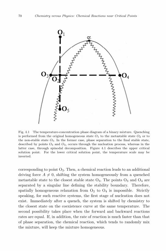
September 11, 2009 10:7 World Scientific Book - 9in x 6in General-nn
70 Chemistry versus Physics: Chemical Reactions near Critical Points
Fig. 4.1 The temperature-concentration phase diagram of a binary mixture. Quenchingis performed from the original homogeneous state O1 to the metastable state O2 or tothe non-stable state O5. In the former case, phase separation to the final stable state,described by points O3 and O4, occurs through the nucleation process, whereas in thelatter case, through spinodal decomposition. Figure 4.1 describes the upper criticalsolution point. For the lower critical solution point, the temperature scale may beinverted.
corresponding to point O3. Then, a chemical reaction leads to an additionaldriving force A �= 0, shifting the system homogeneously from a quenchedmetastable state to the closest stable state O3. The points O3 and O4 areseparated by a singular line defining the stability boundary. Therefore,spatially homogeneous relaxation from O2 to O4 is impossible. Strictlyspeaking, for such reactive systems, the first stage of nucleation does notexist. Immediately after a quench, the system is shifted by chemistry tothe closest state on the coexistence curve at the same temperature. Thesecond possibility takes place when the forward and backward reactionsrates are equal. If, in addition, the rate of reaction is much faster than thatof phase separation, the chemical reaction, which tends to randomly mixthe mixture, will keep the mixture homogeneous.
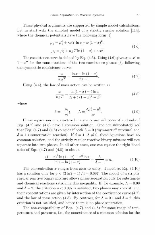
September 11, 2009 10:7 World Scientific Book - 9in x 6in General-nn
Phase Separation in Reactive Systems 71
These physical arguments are supported by simple model calculations.Let us start with the simplest model of a strictly regular solution [114],where the chemical potentials have the following form [3]
µ1 = µ01 + κBT lnx+ ω (1− x)2 ,
µ2 = µ02 + κBT ln (1− x) + ωx2.
(4.6)
The coexistence curve is defined by Eq. (4.5). Using (4.6) gives x ≡ x′ =1 − x′′ for the concentrations of the two coexistence phases [3], followingthe symmetric coexistence curve,
ω
κBT=
lnx− ln (1− x)2x− 1
. (4.7)
Using (4.4), the law of mass action can be written as
ω
κBT=
ln(1− x)− δ lnx
Λ + δ (1− x)2 − x2(4.8)
where
δ = −ν1
ν2; Λ =
δµ01 − µ0
2
ω. (4.9)
Phase separation in a reactive binary mixture will occur if and only ifEqs. (4.7) and (4.8) have a common solution. One can immediately seethat Eqs. (4.7) and (4.8) coincide if both Λ = 0 (“symmetric” mixture) andδ = 1 (isomerization reaction). If δ = 1, Λ �= 0, these equations have nocommon solution, and the strictly regular reactive binary mixture will notseparate into two phases. In all other cases, one can equate the right-handsides of Eqs. (4.7) and (4.8) to obtain
(1− x)2 ln (1− x) − x2 lnxlnx− ln (1− x) =
Λδ − 1
≡ q. (4.10)
The concentration x ranges from zero to unity. Therefore, Eq. (4.10)has a solution only for q < (2 ln 2− 1) /4 = 0.097. The model of a strictlyregular reactive binary mixture allows phase separation only for substancesand chemical reactions satisfying this inequality. If, for example, Λ = 0.09and δ = 2, the criterion q < 0.097 is satisfied, two phases may coexist, andtheir concentrations are given by intersection of the coexistence curve (4.7)and the law of mass action (4.8). By contrast, for Λ = 0.1 and δ = 2, thiscriterion is not satisfied, and hence there is no phase separation.
The non-compatibility of Eqs. (4.7) and (4.8) for some range of tem-peratures and pressures, i.e., the nonexistence of a common solution for the
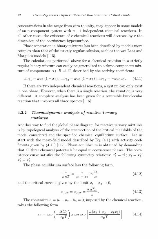
September 11, 2009 10:7 World Scientific Book - 9in x 6in General-nn
72 Chemistry versus Physics: Chemical Reactions near Critical Points
concentrations in the range from zero to unity, may appear in some modelsof an n-component system with n − 1 independent chemical reactions. Inall other cases, the existence of r chemical reactions will decrease by r thedimension of the coexistence hypersurface.
Phase separation in binary mixtures has been described by models morecomplex than that of the strictly regular solution, such as the van Laar andMargules models [115].
The calculations performed above for a chemical reaction in a strictlyregular binary mixture can easily be generalized to a three-component mix-ture of components A+ B � C, described by the activity coefficients
ln γ1 = ωx2 (1− x1) ; ln γ2 = ωx1 (1− x2) ; ln γ3 = −ωx1x2. (4.11)
If there are two independent chemical reactions, a system can only existin one phase. However, when there is a single reaction, the situation is verydifferent. A complete analysis has been given for a reversible bimolecularreaction that involves all three species [116].
4.2.2 Thermodynamic analysis of reactive ternary
mixtures
Another way to find the global phase diagram for reactive ternary mixturesis by topological analysis of the intersection of the critical manifolds of themodel considered and the specified chemical equilibrium surface. Let usstart with the mean-field model described by Eq. (4.1) with activity coef-ficients given by (4.11) [117]. Phase equilibrium is obtained by demandingthat all three chemical potentials be equal in coexistence phases. The coex-istence curve satisfies the following symmetry relations: x′1 = x′1; x
′2 = x′2;
x′3 = x′3.The phase equilibrium surface has the following form,
ω
κBT=
1x1 − x2
lnx1
x2(4.12)
and the critical curve is given by the limit x1 − x2 → 0,
x1,cr = x2,cr =κBTcr
ω. (4.13)
The constraint A = µ1−µ2−µ3 = 0, imposed by the chemical reaction,takes the following form
x3 = exp(−∆G0
κBT
)x1x2 exp
[ω (x1 + x2 − x1x2)
κBT
](4.14)
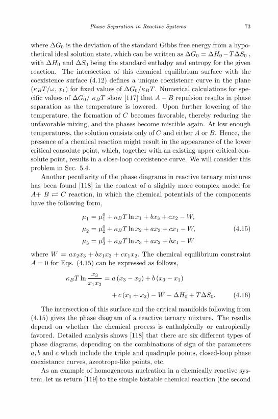
September 11, 2009 10:7 World Scientific Book - 9in x 6in General-nn
Phase Separation in Reactive Systems 73
where ∆G0 is the deviation of the standard Gibbs free energy from a hypo-thetical ideal solution state, which can be written as ∆G0 = ∆H0−T∆S0 ,
with ∆H0 and ∆S0 being the standard enthalpy and entropy for the givenreaction. The intersection of this chemical equilibrium surface with thecoexistence surface (4.12) defines a unique coexistence curve in the plane(κBT/ω, x1) for fixed values of ∆G0/κBT . Numerical calculations for spe-cific values of ∆G0/ κBT show [117] that A−B repulsion results in phaseseparation as the temperature is lowered. Upon further lowering of thetemperature, the formation of C becomes favorable, thereby reducing theunfavorable mixing, and the phases become miscible again. At low enoughtemperatures, the solution consists only of C and either A or B. Hence, thepresence of a chemical reaction might result in the appearance of the lowercritical consolute point, which, together with an existing upper critical con-solute point, results in a close-loop coexistence curve. We will consider thisproblem in Sec. 5.4.
Another peculiarity of the phase diagrams in reactive ternary mixtureshas been found [118] in the context of a slightly more complex model forA+ B � C reaction, in which the chemical potentials of the componentshave the following form,
µ1 = µ01 + κBT lnx1 + bx3 + cx2 −W,
µ2 = µ02 + κBT lnx2 + ax3 + cx1 −W,
µ3 = µ03 + κBT lnx3 + ax2 + bx1 −W
(4.15)
where W = ax2x3 + bx1x3 + cx1x2. The chemical equilibrium constraintA = 0 for Eqs. (4.15) can be expressed as follows,
κBT lnx3
x1x2= a (x3 − x2) + b (x3 − x1)
+ c (x1 + x2)−W −∆H0 + T∆S0. (4.16)
The intersection of this surface and the critical manifolds following from(4.15) gives the phase diagram of a reactive ternary mixture. The resultsdepend on whether the chemical process is enthalpically or entropicallyfavored. Detailed analysis shows [118] that there are six different types ofphase diagrams, depending on the combinations of sign of the parametersa, b and c which include the triple and quadruple points, closed-loop phasecoexistance curves, azeotrope-like points, etc.
As an example of homogeneous nucleation in a chemically reactive sys-tem, let us return [119] to the simple bistable chemical reaction (the second
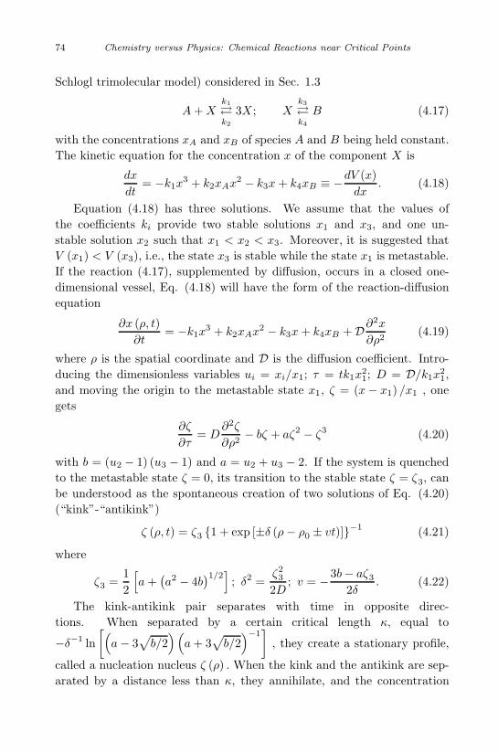
September 11, 2009 10:7 World Scientific Book - 9in x 6in General-nn
74 Chemistry versus Physics: Chemical Reactions near Critical Points
Schlogl trimolecular model) considered in Sec. 1.3
A+Xk1
�k2
3X ; Xk3
�k4
B (4.17)
with the concentrations xA and xB of species A and B being held constant.The kinetic equation for the concentration x of the component X is
dx
dt= −k1x
3 + k2xAx2 − k3x+ k4xB ≡ −dV (x)
dx. (4.18)
Equation (4.18) has three solutions. We assume that the values ofthe coefficients ki provide two stable solutions x1 and x3, and one un-stable solution x2 such that x1 < x2 < x3. Moreover, it is suggested thatV (x1) < V (x3), i.e., the state x3 is stable while the state x1 is metastable.If the reaction (4.17), supplemented by diffusion, occurs in a closed one-dimensional vessel, Eq. (4.18) will have the form of the reaction-diffusionequation
∂x (ρ, t)∂t
= −k1x3 + k2xAx
2 − k3x+ k4xB +D∂2x
∂ρ2(4.19)
where ρ is the spatial coordinate and D is the diffusion coefficient. Intro-ducing the dimensionless variables ui = xi/x1; τ = tk1x
21; D = D/k1x
21,
and moving the origin to the metastable state x1, ζ = (x− x1) /x1 , onegets
∂ζ
∂τ= D
∂2ζ
∂ρ2− bζ + aζ2 − ζ3 (4.20)
with b = (u2 − 1) (u3 − 1) and a = u2 + u3 − 2. If the system is quenchedto the metastable state ζ = 0, its transition to the stable state ζ = ζ3, canbe understood as the spontaneous creation of two solutions of Eq. (4.20)(“kink”-“antikink”)
ζ (ρ, t) = ζ3 {1 + exp [±δ (ρ− ρ0 ± vt)]}−1 (4.21)
where
ζ3 =12
[a+
(a2 − 4b
)1/2]; δ2 =
ζ23
2D; v = −3b− aζ3
2δ. (4.22)
The kink-antikink pair separates with time in opposite direc-tions. When separated by a certain critical length κ, equal to
−δ−1 ln[(a− 3
√b/2)(
a+ 3√b/2)−1
], they create a stationary profile,
called a nucleation nucleus ζ (ρ) . When the kink and the antikink are sep-arated by a distance less than κ, they annihilate, and the concentration

September 11, 2009 10:7 World Scientific Book - 9in x 6in General-nn
Phase Separation in Reactive Systems 75
profile returns to the homogeneous metastable state. When the separationbecomes greater than κ, the kink-antikink pair separates, and the systemevolves toward the homogeneous stable state. Equation (4.21) becomessimplified in the small-amplitude-nucleus limit, when κ → 0 , and the nu-cleation nucleus then becomes
ζ (ρ) =3ba
[1 + cosh (δρ)]−1 =3b2a
sech2
(δρ
2
). (4.23)
Thus far, we have discussed a deterministic system. The influence of ho-mogeneous external white noise and internal chemical fluctuations has beenconsidered [119] in the framework of the extended Kramers approach andthe multivariate master equation, respectively. The nucleation due to theinternal fluctuations is limited to a very narrow region near the transition,and it is difficult to observe this experimentally. The external noise maybe easily greater than the internal noise and, therefore, more important.In addition to the homogeneous nucleation initiated by the fluctuations(considered above), the important problem is non-homogeneous nucleationinitiated, say, by pieces of dust present in solutions.
4.2.3 Kinetics of phase separation
Let us first discuss non-reactive systems. All thermodynamic states withinthe coexistence curve shown by the solid line in Fig. 4.1 belong to two-phase states. Therefore, after a change in temperature (or pressure) frompoint O1 to O2, phase separation will occur and the system will consist oftwo phases described by the thermodynamic condition (4.5) and shown bypoints O3 and O4 in the figure. All states located within the coexistencecurve and close to it are the so-called metastable states. Although theenergy of these states is larger than that of the corresponding two-phasesystem, one needs a finite “push” to pass from the local minimum in energyto the deeper global minimum. Such a “push” is provided by the thermalfluctuations in density for a one-component system and in concentrationfor many-component mixtures. Therefore, these fluctuations are of crucialimportance for the analysis of the decay of a metastable state.
The change of the thermodynamic potential associated with the ap-pearance of the nucleus of the new phase (assumed, for simplicity, to bespherical with radius r) is equal to
∆G (r) = −∆µ43πr3 + 4πσr2 (4.24)
September 11, 2009 10:7 World Scientific Book - 9in x 6in General-nn
76 Chemistry versus Physics: Chemical Reactions near Critical Points
where ∆µ is the energy gain in a stable state compared to a metastablestate, and σ is the surface tension. The first (negative) term in (4.24)encourages phase separation while the second (positive) term prevents it. Itis clear from (4.24) that for small nuclei, ∆G > 0. That is, small nuclei tendto shrink because of their high surface-to-volume ratio. Only nuclei largerthan the critical size rC are energetically favorable. From ∆G/dr = 0, onefinds
rC =2σ∆µ
. (4.25)
The traditional phenomenological approach to the decay of a metastablestate of a pure substance is based on the distribution function W (r, t) ofnuclei of size r at time t. The continuity equation has the form,
∂W
∂t=
∂
∂r
[FW +D
∂W
∂r
]≡ −∂J
∂t(4.26)
where the flux J (r, t) of nuclei along the size axis is determined by twounknown functions F and W . One can reduce [120] the equation(s) of thecritical dynamics to the Langevin equation for the radius of nuclei witha known random force, which can be transformed to the Fokker-Planckequation (4.26) with functions F and D of the form
F (r) = D0
(1r− 1rC
); D (r) =
D0κBT
8πσr2(4.27)
where D0 is the diffusion coefficient far from the critical point.The nucleation process in a binary mixture can be described in analo-
gous fashion [121], [18]. The formation energy of a nucleus containing n1
atoms of component 1 and n2 atoms of component 2 is
∆G =(µ1,n − µ1
)n1 +
(µ2,n − µ2
)n2 + 4πσr2 (4.28)
where µ1 and µ2 are the chemical potentials of the components in thehomogeneous phase, and µ1,n and µ2,n are the corresponding quantities inthe nuclei. The size r of a nucleus is related to its structure by 4πr3/3 =υ1n1 + υ2n2, where υ1 and υ2 are the volumes per atom.
In contrast to a pure substance, the critical nucleus is defined not onlyby its size r, but also by the concentration x = n1/ (n1 + n2). Therefore,the height of the potential barrier is defined by ∂∆G/∂r = ∂∆G/∂x = 0,which gives the following relation between rC and xC of the critical nucleus,
rC = 2σxCυ1 + (1− xC) υ2
xC∆µ1 + (1− xC)∆µ2
(4.29)
September 11, 2009 10:7 World Scientific Book - 9in x 6in General-nn
Phase Separation in Reactive Systems 77
where ∆µi = µi,n − µi.Let us now consider reactive systems. The concentration x changes as
a result of a chemical reaction, which shifts the initial quenched state tothe closest equilibrium state on the coexistence curve. Each intermediatestate corresponds to a different radius of critical nucleus rC (t), increasingtoward the coexistence curve, where rC → ∞. Hence, one has to replacerC by rC (t) everywhere. The latter function can be found from Eq. (4.29)under the assumption of a quasi-static chemical shift. This shift is causedby a chemical reaction, and can be described in the linear approximationby
dx
dt= −x− x
′
τ(4.30)
where τ−1 is the rate of the chemical reaction.Inserting the solution of Eq. (4.30), x − x′ = (x0 − x′) exp
(− tτ
), into
Eq. (4.29), one obtains
rC (t) =2σ [x′′υ1 + (1− x′′) υ2]
κBT [x′′/x′ − (1− x′′) / (1− x′)] (x′ − x′′)≡ r0 exp (t/τ) (4.31)
where we used the coexistence condition (4.5), and retained only the leadinglogarithmic part of the chemical potentials.
The next step is to obtain the Fokker-Planck equation for the distri-bution function W (r, t, x) for nuclei of size r and composition x at timet. We make the approximation that all nuclei which are important forphase separation have the same composition x′′. Therefore, we may omitthe argument x in W (r, t, x). In other words, one assumes that a chemicalreaction brings the path leading to the saddle point closer to that of x = x′′.
Substituting (4.27) and (4.31) into the Fokker-Planck equation ( 4.26),one obtains
∂W
∂t=
∂
∂r
{D0
[1r− 1r0
exp(− tτ
)]W +
D0κBT
8πσr2∂W
∂r
}. (4.32)
To find the approximate solution of this complicated equation, we firstconsider a simplified version, which allows an exact solution. One replacesfunctions F (r) and D (r) in (4.27) by simpler functions which incorporatethe main property of (4.27). According to the physical picture, F (r) ispositive for r < rC and negative for r > rC . Therefore, we approximateF (r) by
F (r) = B (rC − r) . (4.33)
September 11, 2009 10:7 World Scientific Book - 9in x 6in General-nn
78 Chemistry versus Physics: Chemical Reactions near Critical Points
After choosing this form of F (r) , we are no longer free to choosethe second function D (r) . These two functions are not independent be-cause there is no flux in equilibrium, which, according to (4.26), leadsto Weq = exp
[− ∫ drF (r) /D (r)]. On the other hand, by definition,
W = exp (−∆G/kBT ), and, therefore,∫F (r)D (r)
dr =∆GkBT
(4.34)
where ∆G (r) and rC are given by (4.24) and (4.25). A simple calculationyields
D (r) =BkBTrC
8πσr≈ BkBT
8πσ. (4.35)
We keep only the largest term in r−rC in the last equality in (4.35). Using(4.33), (4.31) and (4.35), one obtains the simplified Fokker-Planck equation,
∂W
∂t=
∂
∂r
[B
(r0 exp
(t
τ
)− r)W
]+D0
∂2W
∂r2, (4.36)
where D0 = BkBT/8πσ. Equation (4.36) can be solved exactly by intro-ducing the characteristic function
W (K, t) =∫W (r, t) exp (iKr) dr. (4.37)
The original Fokker-Planck equation (4.26)–(4.27) is thus transformed intoa first-order linear partial differential equation for W (K, t) [122],
∂W
∂t−BK∂W
∂K= −
[D0K
2 + iKBr0 exp(t
τ)]W. (4.38)
To solve this equation, one uses the method of characteristics, withinitial condition
W (r, t = 0) = δ (r − ξ) (4.39)
where ξ is of order of a single molecule (there are no nuclei immediatelyafter a quench). Solving Eq. (4.38) and performing the inverse Fouriertransformation, one obtains the Gaussian distribution function
W (r, t) =1√
4π∆r2exp
[− (r − r)2
2∆r2
](4.40)
with mean value r and variance ∆r2 given by
r = ξ exp (Bt)− Br0τ−1 −B
[exp
(t
τ
)− exp (Bt)
],
∆r2 =D0
2B[exp (2Bt)− 1] . (4.41)
September 11, 2009 10:7 World Scientific Book - 9in x 6in General-nn
Phase Separation in Reactive Systems 79
Two characteristic times, B−1 and τ , are associated with transient pro-cesses and chemical reactions, respectively. However, the solution (4.40)diverges with time, so that Eq. (4.36) does not have a steady-state solu-tion. Hence, instead of the exact solution, one has to use the approximatesolution.
One can find [122] the appropriate solution of Eq. (4.36), but we preferto find the solution of the original equations (4.26) and (4.27), assum-ing that B−1 is very small [123]. This assumption permits us to neglecttransient processes, and, for B−1 < τ , restrict attention to those solu-tions of (4.36) which supply the quasi-static flux Jqss (t) independent onthe size of the nuclei. We consider the quasi-steady-state regime whichis established after the transients disappear. The quasi-steady-state so-lution Wqss [r, rC (t)] does not have an explicit time dependence, so that∂Wqss/∂t = 0, and the Fokker-Planck equation (4.32) can be rewritten as
D0
[1r− 1r0
exp(− tτ
)]Wqss +
D0κBT
8πσr2∂Wqss
∂r≡ Jqss
(t
τ
). (4.42)
The quasi-steady-state flux Jqss reduces to the steady-state flux Jss whenthe chemical reaction is absent,
Jqss
(t
τ= 0)
= Jss. (4.43)
There is no stationary state for the reactive system considered here.Therefore, one is forced to give a new definition to the lifetime of ametastable state in reactive systems. The simplest generalization is thetime required to produce one critical nucleus
Tch∫0
dt Jqss (t) = 1. (4.44)
For the time-independent case, Jqss is replaced by Jss, according to(4.43), and Tch is replaced by the lifetime of the metastable state in thenon-reactive system, T0 = J−1
ss .Let us now turn to the solution of Eq. (4.42). The boundary conditions
for this equation are determined by the requirements that the distributionof nuclei of minimal size ξ will be the equilibrium distribution, and the totalnumber of nuclei in the system is bounded,
Wqss (ξ) = Weq (ξ) ; Wqss (r →∞) = 0 (4.45)
where Weq corresponds to zero flux.
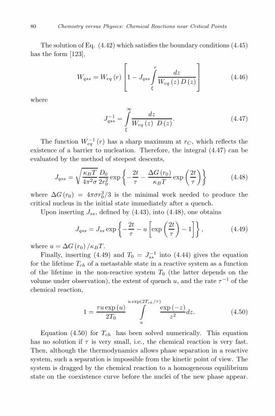
September 11, 2009 10:7 World Scientific Book - 9in x 6in General-nn
80 Chemistry versus Physics: Chemical Reactions near Critical Points
The solution of Eq. (4.42) which satisfies the boundary conditions (4.45)has the form [123],
Wqss = Weq (r)
1− Jqss
r∫ξ
dz
Weq (z)D (z)
(4.46)
where
J−1qss =
∞∫ξ
dz
Weq (z) D (z). (4.47)
The function W−1eq (r) has a sharp maximum at rC , which reflects the
existence of a barrier to nucleation. Therefore, the integral (4.47) can beevaluated by the method of steepest descents,
Jqss =
√κBT
4π2σ
D0
2r20exp
{−2tτ− ∆G (r0)
κBTexp
(2tτ
)}(4.48)
where ∆G (r0) = 4πσr30/3 is the minimal work needed to produce thecritical nucleus in the initial state immediately after a quench.
Upon inserting Jss, defined by (4.43), into (4.48), one obtains
Jqss = Jss exp{−2tτ− u
[exp
(2tτ
)− 1]}
, (4.49)
where u = ∆G (r0) /κBT .Finally, inserting (4.49) and T0 = J−1
ss into (4.44) gives the equationfor the lifetime Tch of a metastable state in a reactive system as a functionof the lifetime in the non-reactive system T0 (the latter depends on thevolume under observation), the extent of quench u, and the rate τ−1 of thechemical reaction,
1 =τu exp (u)
2T0
u exp(2Tch/τ)∫u
exp (−z)z2
dz. (4.50)
Equation (4.50) for Tch has been solved numerically. This equationhas no solution if τ is very small, i.e., the chemical reaction is very fast.Then, although the thermodynamics allows phase separation in a reactivesystem, such a separation is impossible from the kinetic point of view. Thesystem is dragged by the chemical reaction to a homogeneous equilibriumstate on the coexistence curve before the nuclei of the new phase appear.
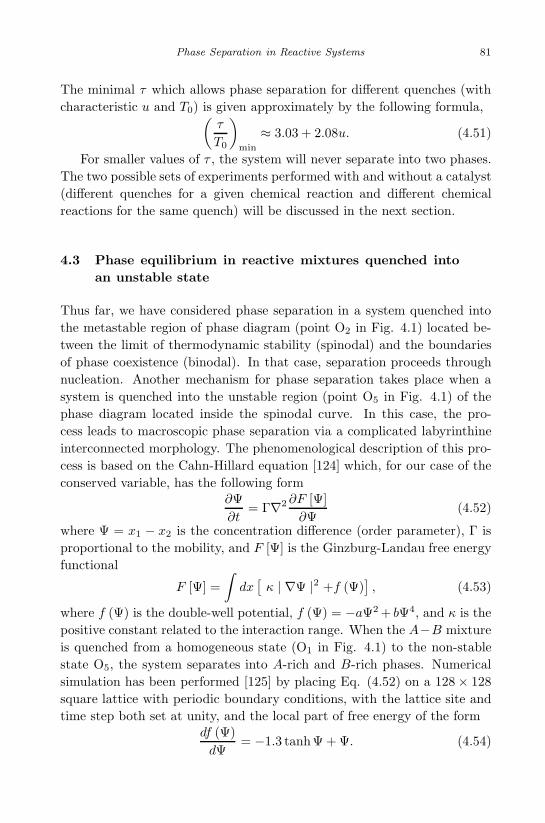
September 11, 2009 10:7 World Scientific Book - 9in x 6in General-nn
Phase Separation in Reactive Systems 81
The minimal τ which allows phase separation for different quenches (withcharacteristic u and T0) is given approximately by the following formula,(
τ
T0
)min
≈ 3.03 + 2.08u. (4.51)
For smaller values of τ , the system will never separate into two phases.The two possible sets of experiments performed with and without a catalyst(different quenches for a given chemical reaction and different chemicalreactions for the same quench) will be discussed in the next section.
4.3 Phase equilibrium in reactive mixtures quenched intoan unstable state
Thus far, we have considered phase separation in a system quenched intothe metastable region of phase diagram (point O2 in Fig. 4.1) located be-tween the limit of thermodynamic stability (spinodal) and the boundariesof phase coexistence (binodal). In that case, separation proceeds throughnucleation. Another mechanism for phase separation takes place when asystem is quenched into the unstable region (point O5 in Fig. 4.1) of thephase diagram located inside the spinodal curve. In this case, the pro-cess leads to macroscopic phase separation via a complicated labyrinthineinterconnected morphology. The phenomenological description of this pro-cess is based on the Cahn-Hillard equation [124] which, for our case of theconserved variable, has the following form
∂Ψ∂t
= Γ∇2 ∂F [Ψ]∂Ψ
(4.52)
where Ψ = x1 − x2 is the concentration difference (order parameter), Γ isproportional to the mobility, and F [Ψ] is the Ginzburg-Landau free energyfunctional
F [Ψ] =∫dx[κ | ∇Ψ |2 +f (Ψ)
], (4.53)
where f (Ψ) is the double-well potential, f (Ψ) = −aΨ2 + bΨ4, and κ is thepositive constant related to the interaction range. When the A−B mixtureis quenched from a homogeneous state (O1 in Fig. 4.1) to the non-stablestate O5, the system separates into A-rich and B-rich phases. Numericalsimulation has been performed [125] by placing Eq. (4.52) on a 128× 128square lattice with periodic boundary conditions, with the lattice site andtime step both set at unity, and the local part of free energy of the form
df (Ψ)dΨ
= −1.3 tanhΨ + Ψ. (4.54)
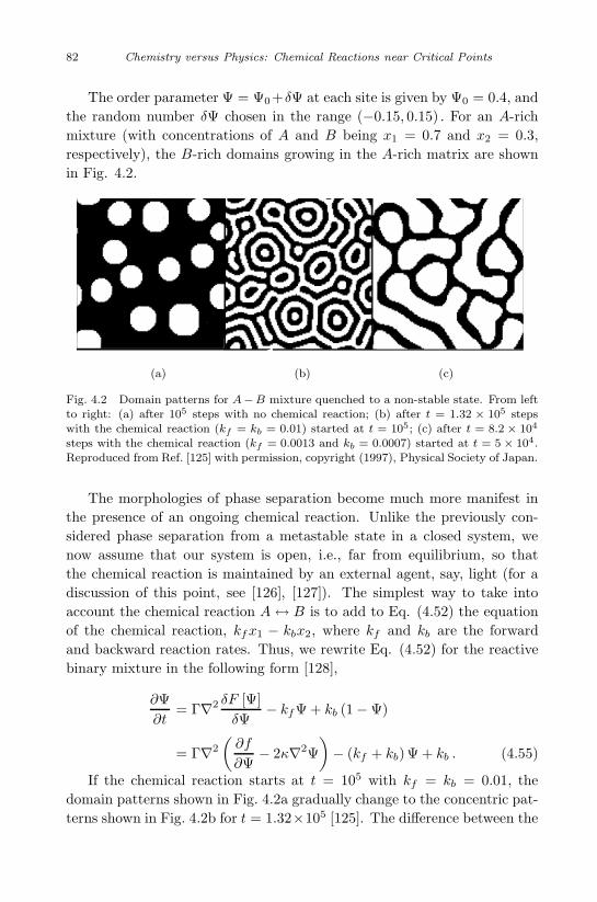
September 11, 2009 10:7 World Scientific Book - 9in x 6in General-nn
82 Chemistry versus Physics: Chemical Reactions near Critical Points
The order parameter Ψ = Ψ0+δΨ at each site is given by Ψ0 = 0.4, andthe random number δΨ chosen in the range (−0.15, 0.15) . For an A-richmixture (with concentrations of A and B being x1 = 0.7 and x2 = 0.3,respectively), the B-rich domains growing in the A-rich matrix are shownin Fig. 4.2.
(a) (b) (c)
Fig. 4.2 Domain patterns for A−B mixture quenched to a non-stable state. From leftto right: (a) after 105 steps with no chemical reaction; (b) after t = 1.32 × 10⁵ stepswith the chemical reaction (kf = kb = 0.01) started at t = 105; (c) after t = 8.2 × 10⁴
steps with the chemical reaction (kf = 0.0013 and kb = 0.0007) started at t = 5 × 10⁴.Reproduced from Ref. [125] with permission, copyright (1997), Physical Society of Japan.
The morphologies of phase separation become much more manifest inthe presence of an ongoing chemical reaction. Unlike the previously con-sidered phase separation from a metastable state in a closed system, wenow assume that our system is open, i.e., far from equilibrium, so thatthe chemical reaction is maintained by an external agent, say, light (for adiscussion of this point, see [126], [127]). The simplest way to take intoaccount the chemical reaction A↔ B is to add to Eq. (4.52) the equationof the chemical reaction, kfx1 − kbx2, where kf and kb are the forwardand backward reaction rates. Thus, we rewrite Eq. (4.52) for the reactivebinary mixture in the following form [128],
∂Ψ∂t
= Γ∇2 δF [Ψ]δΨ
− kfΨ + kb (1−Ψ)
= Γ∇2
(∂f
∂Ψ− 2κ∇2Ψ
)− (kf + kb)Ψ + kb . (4.55)
If the chemical reaction starts at t = 105 with kf = kb = 0.01, thedomain patterns shown in Fig. 4.2a gradually change to the concentric pat-terns shown in Fig. 4.2b for t = 1.32×10⁵ [125]. The difference between the
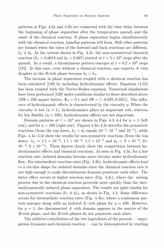
September 11, 2009 10:7 World Scientific Book - 9in x 6in General-nn
Phase Separation in Reactive Systems 83
patterns in Figs. 4.2a and 4.2b are connected with the time delay betweenthe beginning of phase separation after the temperature quench and theonset of the chemical reaction. If phase separation begins simultaneouslywith the chemical reaction, lamellar patterns will form. Still other patternsare formed when the rates of the forward and back reactions are different,kf �= kb. In the system shown in Fig. 4.2c, the non-symmetrical chemicalreaction (kf = 0.0013 and kb = 0.007) started at t = 5×10⁴ steps after thequench. As a result, a bicontinuous pattern emerges at t = 8.2× 10⁴ steps[125]. In this case, even without a chemical reaction, one expects A -richdroplets in the B-rich phase because kb > kf .
The increase in phase separation coupled with a chemical reaction hasbeen calculated [129] by including hydrodynamic effects. Equation (4.55)has been coupled with the Navier-Stokes equation. Numerical simulationshave been performed [129] under conditions similar to those described above(256 × 256 square lattice, Ψ0 = 0.1 and δΨ = (−0.025, 0.025)). The influ-ence of hydrodynamic effects is characterized by the viscosity η. When theviscosity is low (η = 1), hydrodynamics plays an important role, whereasfor low fluidity (η = 100), hydrodynamic effects are not important.
Domain patterns at t = 104 are shown in Figs. 4.3–4.4 for η = 1 (leftrow), and for η = 100 (right row). Figures 4.3a–4.3c describe the symmetricreactions (from the top down, kf = kb equals 10−4, 10−3 and 10−2), whileFigs. 4.4a–4.4c show the results for non-symmetric reactions (from the topdown: kf = 1.1 × 10⁻⁴; 1.1 × 10⁻³; 1.1 × 10⁻² and kb = 9 × 10⁻⁵; 9×10⁻⁴; 9 × 10⁻³). These figures clearly show the competition between hy-drodynamics effects and chemical reactions. As seen in Fig. 4.3a, for a lowreaction rate, isolated domains become more circular under hydrodynamicflow. For intermediate reaction rates (Fig. 4.3b), hydrodynamic effects leadto a circular shape for isolated domains since the chemical reaction rate isnot high enough to make discontinuous domains penetrate each other. Thelatter effect occurs at higher reaction rates (Fig. 4.3c), where the mixingprocess due to the chemical reaction proceeds more quickly than the ther-modynamically induced phase separation. The results are quite similar fornon-symmetric reactions (kf �= kb), as shown in Fig. 4.4. Some differenceoccurs for intermediate reaction rates (Fig. 4.4b), where a continuous pat-tern emerges along with an isolated A -rich phase for η = 100. However,for η = 1, the disconnected A -rich domain appears in the matrix of theB-rich phase, and the B-rich phases do not penetrate each other.
The additive contribution of the two ingredients of the process — segre-gation dynamics and chemical reaction — can be demonstrated by starting
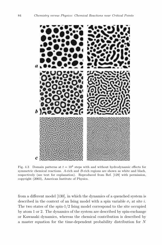
September 11, 2009 10:7 World Scientific Book - 9in x 6in General-nn
84 Chemistry versus Physics: Chemical Reactions near Critical Points
Fig. 4.3 Domain patterns at t = 104 steps with and without hydrodynamic effects forsymmetric chemical reactions. A-rich and B-rich regions are shown as white and black,respectively (see text for explanation). Reproduced from Ref. [129] with permission,copyright (2003), American Institute of Physics.
from a different model [130], in which the dynamics of a quenched system isdescribed in the context of an Ising model with a spin variable σi at site i.The two states of the spin-1/2 Ising model correspond to the site occupiedby atom 1 or 2. The dynamics of the system are described by spin-exchangeor Kawasaki dynamics, whereas the chemical contribution is described bya master equation for the time-dependent probability distribution for N
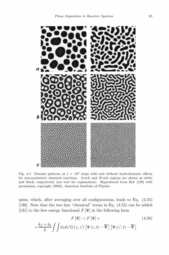
September 11, 2009 10:7 World Scientific Book - 9in x 6in General-nn
Phase Separation in Reactive Systems 85
Fig. 4.4 Domain patterns at t = 104 steps with and without hydrodynamic effectsfor non-symmetric chemical reactions. A-rich and B-rich regions are shown as whiteand black, respectively (see text for explanation). Reproduced from Ref. [129] withpermission, copyright (2003), American Institute of Physics
spins, which, after averaging over all configurations, leads to Eq. (4.55)[130]. Note that the two last “chemical” terms in Eq. (4.55) can be added[131] to the free energy functional F [Ψ] in the following form
F [Ψ]→ F [Ψ] + (4.56)
+kf + kb
2
∫ ∫dzdz′G (z, z′)
[Ψ (z, t)−Ψ
] [Ψ (z′, t)−Ψ
]
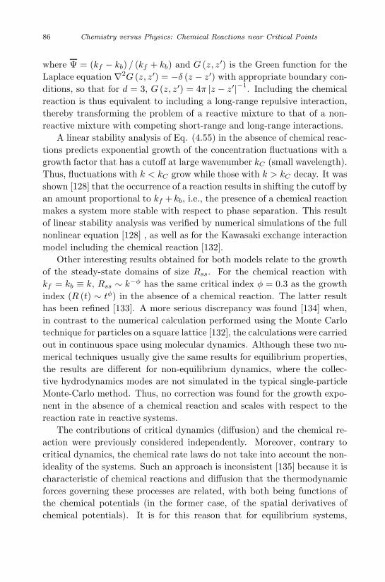
September 11, 2009 10:7 World Scientific Book - 9in x 6in General-nn
86 Chemistry versus Physics: Chemical Reactions near Critical Points
where Ψ = (kf − kb) / (kf + kb) and G (z, z′) is the Green function for theLaplace equation ∇2G (z, z′) = −δ (z − z′) with appropriate boundary con-ditions, so that for d = 3, G (z, z′) = 4π |z − z′|−1. Including the chemicalreaction is thus equivalent to including a long-range repulsive interaction,thereby transforming the problem of a reactive mixture to that of a non-reactive mixture with competing short-range and long-range interactions.
A linear stability analysis of Eq. (4.55) in the absence of chemical reac-tions predicts exponential growth of the concentration fluctuations with agrowth factor that has a cutoff at large wavenumber kC (small wavelength).Thus, fluctuations with k < kC grow while those with k > kC decay. It wasshown [128] that the occurrence of a reaction results in shifting the cutoff byan amount proportional to kf + kb, i.e., the presence of a chemical reactionmakes a system more stable with respect to phase separation. This resultof linear stability analysis was verified by numerical simulations of the fullnonlinear equation [128] , as well as for the Kawasaki exchange interactionmodel including the chemical reaction [132].
Other interesting results obtained for both models relate to the growthof the steady-state domains of size Rss. For the chemical reaction withkf = kb ≡ k, Rss ∼ k−φ has the same critical index φ = 0.3 as the growthindex (R (t) ∼ tφ) in the absence of a chemical reaction. The latter resulthas been refined [133]. A more serious discrepancy was found [134] when,in contrast to the numerical calculation performed using the Monte Carlotechnique for particles on a square lattice [132], the calculations were carriedout in continuous space using molecular dynamics. Although these two nu-merical techniques usually give the same results for equilibrium properties,the results are different for non-equilibrium dynamics, where the collec-tive hydrodynamics modes are not simulated in the typical single-particleMonte-Carlo method. Thus, no correction was found for the growth expo-nent in the absence of a chemical reaction and scales with respect to thereaction rate in reactive systems.
The contributions of critical dynamics (diffusion) and the chemical re-action were previously considered independently. Moreover, contrary tocritical dynamics, the chemical rate laws do not take into account the non-ideality of the systems. Such an approach is inconsistent [135] because it ischaracteristic of chemical reactions and diffusion that the thermodynamicforces governing these processes are related, with both being functions ofthe chemical potentials (in the former case, of the spatial derivatives ofchemical potentials). It is for this reason that for equilibrium systems,
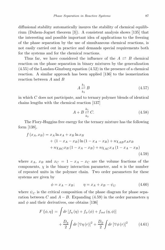
September 11, 2009 10:7 World Scientific Book - 9in x 6in General-nn
Phase Separation in Reactive Systems 87
diffusional stability automatically insures the stability of chemical equilib-rium (Duhem-Joguet theorem [3]). A consistent analysis shows [135] thatthe interesting and possible important idea of applications to the freezingof the phase separation by the use of simultaneous chemical reactions, isnot easily carried out in practice and demands special requirements bothfor the systems and for the chemical reactions.
Thus far, we have considered the influence of the A � B chemicalreaction on the phase separation in binary mixtures by the generalization(4.55) of the Landau-Ginzburg equation (4.52) in the presence of a chemicalreaction. A similar approach has been applied [136] to the isomerizationreaction between A and B
Ak1
�k2
B (4.57)
in which C does not participate, and to ternary polymer blends of identicalchains lengths with the chemical reaction [137]
A+Bk1
�k2
C. (4.58)
The Flory-Huggins free energy for the ternary mixture has the followingform [138],
f (xA, xB) = xA lnxA + xB lnxB
+ (1− xA − xB) ln (1− xA − xB) + nχABxAxB
+nχBCxB (1− xA − xB) + nχACxA (1− xA − xB)
(4.59)
where xA, xB and xC = 1 − xA − xC are the volume fractions of thecomponents, χ is the binary interaction parameter, and n is the numberof repeated units in the polymer chain. Two order parameters for thesesystems are given by
φ = xA − xB ; η = xA + xB − ψC (4.60)
where ψC is the critical composition of the phase diagram for phase sepa-ration between C and A−B. Expanding (4.59) in the order parameters ηand φ and their derivatives, one obtains [136]
F {φ, η} =∫dr [fη (η) + fφ (φ) + fint (η, φ)]
+Dη
2
∫dr [�η (r)]2 +
Dφ
2
∫dr [�φ (r)]2 (4.61)
September 11, 2009 10:7 World Scientific Book - 9in x 6in General-nn
88 Chemistry versus Physics: Chemical Reactions near Critical Points
where Dη and Dφ are phenomenological parameters related to the surfaceenergy, and
fη (η) = −12c1η
2 +14c2η
4
fφ (φ) = −12c3φ
2 +14c4φ
4
fint (η, φ) = c5ηφ− 12c6ηφ
2 +12c7η
2φ2
(4.62)
where the ci are functions of the coefficients χ and ψC (for details, see [136],[137]). The equation of motion for the order parameters η and φ (Landau-Ginzburg equations generalized to a chemically reactive ternary mixture)have a slightly different form for the chemical reactions (4.57) and (4.58).In the former case,
∂η
∂t= Mη�2 δF {φ, η}
δη,
∂φ
∂t= Mφ�2 δF {φ, η}
δφ− (k1 + k2)φ
− (k1 − k2) η − (k1 − k2)ψC (4.63)
whereas in the latter case,
∂η
∂t= Mη�2 δF{φ,η}
δη + 2k2ψC − 2k1xAxB,
∂φ
∂t= Mφ�2 δF{φ,η}
δφ ,
(4.64)
where Mφ and Mη are the mobility coefficients. For simplicity, the follow-ing forms of the functions fη (η) and fφ (φ) have been used in numericalsimulations,
dfη
dη= Aη tanh η − η; dfφ
dφ= Aφ tanhφ− φ (4.65)
where Aη and Aφ are phenomenological parameters which are inverselyproportional to temperature.
Numerical simulations show [136] that for the isomerization reaction(4.57), a difference between phase separation in a ternary mixture and ina binary mixture, related to the availability of the third inert component,leads to the existence of a multiple-phase transition. Otherwise, the dy-namics of phase separation in binary and ternary mixtures is quite similar.

September 11, 2009 10:7 World Scientific Book - 9in x 6in General-nn
Phase Separation in Reactive Systems 89
For reaction (4.58), the separation dynamics depends on the competitionbetween the chemical reaction and phase separation [137]. In the case of arelatively large reaction rate constant, the effect of a chemical reaction isdominant, phase separation between C and A − B is inhibited, and phaseseparation occurs between A and B. As the phase separation of A andB proceeds, C decomposes into A and B rapidly, resulting in the phasepattern of small amount of C distributed along the interface between A-rich and B-rich domains. As the reaction rate gradually decreases, theeffect of the chemical reaction diminishes. In the later stages of phaseseparation, the concentration of C increases as the rate constant of thechemical reaction decreases, and the C-rich phase changes from disperseddroplets to a continuous thin phase. In the next section, we consider thedissociation reaction which is a special type of chemical reaction in a ternarymixture.
4.4 Thermodynamics of a three-component plasma with adissociative chemical reaction
Order-disorder phase transitions and critical phenomena in electricallyneutral systems are due to the competition between repulsive and at-tractive forces. When charged particles appear due to the dissociation-recombination reaction, they give rise to new attractive forces (the Coulombinteraction between ions, which is, on average, an attractive interaction)and repulsive forces (say, the hard-core interaction at short distances).These new competing forces result in an additional first-order phase tran-sition in a three-component plasma with a critical point. The coexistingphases for a new phase transition resulting from the chemical reaction aredetermined by Eqs. (4.12) and (4.16). It has been proposed [85], [114] thatsuch arguments can be used to explain some experiments in metallic vaporsat high pressures and in metal-ammonia solutions.
Metal-ammonia solutions are a type of system in which a small increaseof the concentration of metal results in a huge increase of electroconduc-tivity, manifesting a transition from nonmetallic to metallic conductivity.Metallic vapors are another example of the latter behavior. The continuousdecrease in the density of metals with heating above the critical temperaturecauses the transition into the nonmetallic state and a significant decreaseof the electric conductivity.
The most general explanation of the nature of this transition was given
September 11, 2009 10:7 World Scientific Book - 9in x 6in General-nn
90 Chemistry versus Physics: Chemical Reactions near Critical Points
by Mott [139], who proposed the following elegant physical argument. Mottargued that changing the number density n of charges interacting by ascreened Coulomb interaction eliminates the bound states when aBn
−1/3 ≈0.25, and hence the system will become metallic. Here, aB is the Bohrradius in the medium. Despite the generality of the Mott criterion, not allmetal-nonmetal transitions can be explained in this way. Sometimes thetransition takes place at a density lower than that predicted by the Mottcriterion [140]; in other systems, there is more than one transition. Let usconsider two examples in more detail.
The liquid-gas critical point of mercury occurs at the densityρC = 5.77 g/cm3 (pC = 1670 Bar, TC = 1750 K). Afterwards, a metal-nonmetal transition takes place at ρ ≈ 9 g/cm3. It is generally accepted(see, however, [141]) that the latter transition is explained by the Mott cri-terion. However, a dielectric anomaly has been found [142] at the densityρ ≈ 3 g/cm3. This was interpreted as a transition from a weakly ionizedmercury plasma to a new inhomogeneous phase of charged droplets. Thistransition, probably of first order, occurs at densities much lower than thosegiven by Mott, and therefore requires an explanation.
The second example is even more conclusive. The heat capacity ofsodium-ammonia solution has been measured [143] for three different mo-lar fractions of metal (X = 0.045, 0.0462, and 0.0631). Starting at lowtemperatures, the heat capacity shows a jump across the liquid-gas sepa-ration curve of this mixture. Upon further heating, two additional jumpsin the heat capacity occur at two distinct temperatures above the criticaltemperature. The changes in slope of the electromotive force take placeat the same temperatures [144] providing additional evidence for a first-order phase transition above the liquid-gas critical point. Experimentalobservation of this new phase transition is very difficult because of the verysmall density differences between the two phases and the existence of slowdiffusion processes. The former requires extreme homogeneity of the tem-perature, and the latter results in very long relaxation times. We believethat these and other experimental problems prevent the observation of thisnew thermodynamic phase transition for other systems, while its existenceseems obvious for a broad class of systems. In addition to metal-ammoniasolutions, one can mention molten salts, weak electrolytes, solutions of met-als in their salts, electron-hole plasmas in optically excited semiconductors,etc.
A ternary mixture with an ionization reaction is another example ofphase separation in reactive systems [114]. Let us consider a system com-
September 11, 2009 10:7 World Scientific Book - 9in x 6in General-nn
Phase Separation in Reactive Systems 91
posed of neutral particles which are partially dissociated into positive andnegative charges. Assume that the Gibbs free energy has the followingform,
G = NAµA,0 +NIµI,0 +Neµe,0
+NAκBT lnxA + 2NIκBT lnxI +NII + µ0NIxαI (4.66)
where NA is the number of neutral particles, NI (Ne) is the number ofions (electrons), I is the ionization potential, and xA ≡ NA/ (NA + 2NI) =1− 2x. Electroneutrality requires that NI = Ne.
The first three terms in Eq. (4.66) describe the ideal gases of the par-ticles. The next two terms are the entropy, the sixth term describes theionization process, and the last term represents the interaction between thecharged particles. We will later make the Debye-Huckel approximation,
α =12; µ0 = − e3
3κBT
( p
2ε3π2
)1/2
. (4.67)
One can formulate the Debye-Huckel approximation using either theGibbs or the Helmholtz free energy. If one switches from one free energy tothe other by using the ideal gas equation of state in the correction term, theDebye-Huckel approximation is slightly different. We here use the Gibbsfree energy, and our equation (4.67) follows from Eqs. (94.1) and (75.14)of Landau and Lifshitz [4].
The chemical potentials of the neutral and charged particles can beeasily found from (4.66),
µA = µA,0 + κBT lnxA − αµ0xα+1,
µq ≡ µI + µe = µI,0 + µe,0
+ 2κBT lnx+ µ0
[(α+ 1)xα − 2αxα+1
]+ I.
(4.68)
In order to obtain the coexistence curve, one equates the chemical potentialsin the two phases, analogously to Eq. (4.5). Solving these two equationsfor αµ0/κBT yields
ln (1− 2x′)− ln (1− 2x′′)(x′)α+1 − (x′′)α+1
=2α (ln x′ − lnx′′)
2α[(x′)α+1 − (x′′)α+1
]− (α+ 1) [(x′)α − (x′′)α]
. (4.69)
One can easily verify that Eq. (4.69) gives the following relation betweenthe charge concentrations in the coexisting phases,
September 11, 2009 10:7 World Scientific Book - 9in x 6in General-nn
92 Chemistry versus Physics: Chemical Reactions near Critical Points
(x′
x′′
)α
=1− 2x′′
1− 2x′. (4.70)
For the Debye-Huckel interaction (4.67), the coexistence curve has thefollowing form,
x′ =[1− x′′ − (2− 3x′′)1/2 (x′′)1/2
]1/2
,
−[
e3
6 (κBT )2
]( p
2ε3π2
)1/2
=lnx′ − lnx′′
(x′)3/2 − (x′′)3/2. (4.71)
If the dissociation reaction A � I + e takes place, one has to add therestriction stemming from the law of mass action, µA − µI − µe = 0. Using(4.67) and (4.68), one can write the latter equation in the following form
µ0A − µ0
I − µ0e − I + κBT ln
1− 2xx2
+µ0
2
(3x1/2 − x3/2
)= 0. (4.72)
Neglecting the difference between the mass of atom and ion, we putµ0
A = µ0I . Furthermore, using the well-known expression for an ideal gas of
electrons, one obtains from (4.72),
ln
[p
κBT
(2π�
2
meκBT
)3/2]
+I
κBT− ln
(1− 2xx2
)
−[e3/6 (κBT )2
] ( p
2ε3π2
)1/2 (3x1/2 − x3/2
)= 0. (4.73)
Equation (4.73) gives the required restriction on the parameters of thecoexisting phases resulting from the chemical reaction. One has to findthe simultaneous solutions of Eqs. (4.71) and (4.73). Since one cannotsolve these equations analytically, one adopts the following approximateprocedure: for given I and ε, one starts from some x′, which gives x′′ andtwo equations for T and p (for details, see [114]).
September 11, 2009 10:7 World Scientific Book - 9in x 6in General-nn
Chapter 5
Comments on the Geometry of thePhase Diagram of a Reaction Mixture
5.1 Solubility in supercritical fluids
The properties of fluids slightly above their critical points (“supercriticalfluids”) came to the attention of researchers more than a century ago, be-cause of their many technological applications. These include supercriticalextraction [145], supercritical chromatography [146] , and the strong pres-sure (or temperature) effect on the reaction rate [26]. We concentrate hereon the phenomenon of enhanced solubility of solids in supercritical fluids(“supercritical extraction”) [70]. The technological advantages of this phe-nomenon have aroused great interest in the chemical engineering commu-nity. Indeed, this interest is reflected in the existence of a journal (Journalof Supercritical Fluids), books ([147], [148], among others), and hundredsof scientific and technological articles.
Figure 5.1 displays a typical example of the phenomenon. Depicted isthe mole fraction of naphthalene dissolved in ethylene as a function of thepressure for various fixed supercritical temperatures [149]. (The criticaltemperature and pressure of the solvent are 11◦C and 51.2 atm.) The sameeffect was found for many other substances. Figure 5.1 shows that for everyisotherm, there is a region of pressure where small changes in pressure resultin a huge increase in solubility. Moreover, the slope of this increase becomeslarger as T approaches TC .
The thermodynamic analysis of this phenomenon (similar to that per-formed in Sec. 2.5) must be appropriate to the experimental setup whichallows a solid to equilibrate with a supercritical fluid at a given temper-ature and pressure. Denote the fluid component (solvent) by subscript 1,and the solid component (solute) by subscript 2. Denoting the solid phaseby superscript s and the fluid phase by f, we have Xs
2 = 1, where X2 is
93
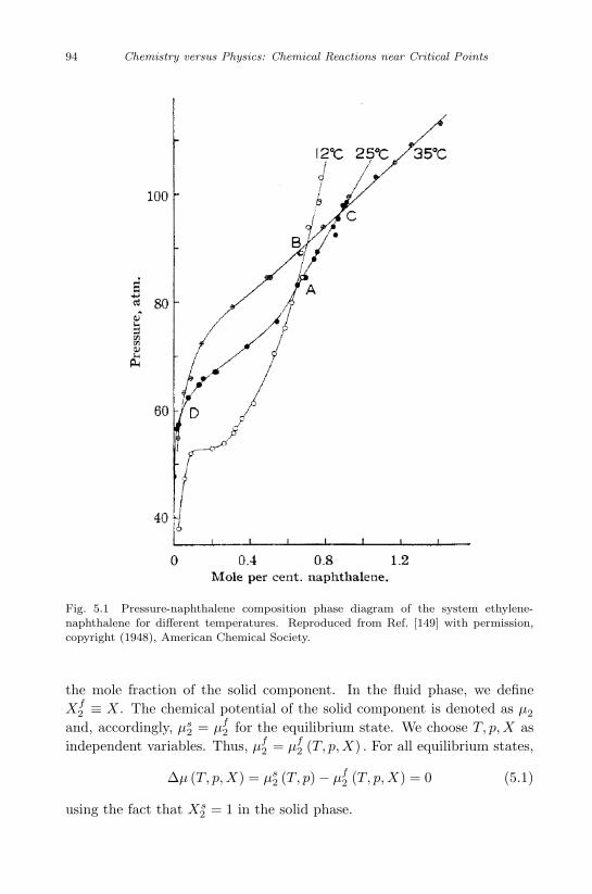
September 11, 2009 10:7 World Scientific Book - 9in x 6in General-nn
94 Chemistry versus Physics: Chemical Reactions near Critical Points
Fig. 5.1 Pressure-naphthalene composition phase diagram of the system ethylene-naphthalene for different temperatures. Reproduced from Ref. [149] with permission,copyright (1948), American Chemical Society.
the mole fraction of the solid component. In the fluid phase, we defineXf
2 ≡ X . The chemical potential of the solid component is denoted as µ2
and, accordingly, µs2 = µf
2 for the equilibrium state. We choose T, p,X asindependent variables. Thus, µf
2 = µf2 (T, p,X) . For all equilibrium states,
∆µ (T, p,X) = µs2 (T, p)− µf
2 (T, p,X) = 0 (5.1)
using the fact that Xs2 = 1 in the solid phase.
September 11, 2009 10:7 World Scientific Book - 9in x 6in General-nn
Comments on the Geometry of the Phase Diagram of a Reaction Mixture 95
Consider isothermal changes of pressure along the equilibrium line,
d [∆µ (T, p,X)] =(∂µs
2
∂p
)T
dp
−(∂µf
2
∂p
)T,X
dp−(∂µf
2
∂X
)T,p
dX = 0 (5.2)
Using the definition of the molar volume of the solid υs = (∂µs2/∂p)T and
of the partial volume of the solute in the fluid phase υ =(∂µf
2/∂p)
T,X,
one can rewrite Eq. (5.2) in the following form(∂X
∂p
)T,equil.line
=υs − υ(
∂µf2/∂X
)T,p
. (5.3)
This result is completely general, and will form the basis of the subse-quent analysis. One can already see from (5.3) that near the critical points,the denominator goes to zero, leading to the strong divergence of the left-hand side of this equation, which corresponds to the graphs shown in Fig.5.1.
It is instructive to examine Eq. (5.3) far from criticality. Using thewell-known form of the chemical potential of dilute solutions,
µf2 = µf
2,0 (T, p) +RT lnX, (5.4)
one obtains from (5.3),(∂ lnX∂p
)T,equil.line
=υs − υRT
. (5.5)
Far from criticality, the fluid mixture is ideal, and the partial volumeof the solute υ is much larger than its molar volume in the solid phase,υ >> υs. Therefore, (∂ lnX, ∂p)T,equil.line < 0, i.e., X decreases as pincreases. In addition,(
∂2 lnX∂p2
)T,equil.line
=1RT
[(∂υs
∂p
)T
−(∂υ
∂p
)T,X
](5.6)
because υ does not depend on X in this region of pressure. Therefore,the derivatives along the equilibrium line coincide with the derivatives at apoint. Since |(∂υs/∂p)T | <<
∣∣∣(∂υ/∂p)T,X
∣∣∣ (i.e., the solid compressibility isalmost zero), the equilibrium isothermal curve X (p) has positive curvaturefor low pressures. Since (∂υ/∂p)T,X is negative but much larger in absolutevalue than (∂υs/∂p)T , υ decreases with increasing pressure and a minimum
September 11, 2009 10:7 World Scientific Book - 9in x 6in General-nn
96 Chemistry versus Physics: Chemical Reactions near Critical Points
in the curve X (p) occures when υ = υs. From this point onward, X (p) isan increasing function unless it reaches the critical region.
Let us now return to the problem of solubility in the critical region.One can immediately see that the chemical potential of a solute in dilutesolutions cannot have the usual form (5.4) near the critical points, becauseone cannot satisfy Eq. (1.2) using the potential of the form (5.4). ln thissense [150], the critical dilute solution is not “dilute”! In deriving Eq.(5.4), it was assumed that one can neglect the interaction between soluteparticles because of the initial assumption that the solution is very weak.However, this is incorrect near the critical point because long-range corre-lations (1.5) cause the effective “interaction” between the solute particlesto be important even for dilute solutions.
Let us obtain the correct expression for the chemical potential µs ofa solute in a binary mixture (calculations for many-component mixturesare quite analogous). Differentiating the Gibbs-Duhem relation [3] υ =υ1X+υ2 (1−X) for the partial volumes υ1 and υ2, with respect to X, andeliminating υ2, yields
υ1 = υ + (1−X)(∂υ
∂X
)T,p
. (5.7)
However, the partial volume is related [3] to the chemical potential υ1 =(∂µs/∂p)T,x. Integrating the latter formula, and using (5.4) for the idealgas as a reference system, gives
µs (T, p,X) = RT lnX +∫ p
0
(υ1 − υid) dp. (5.8)
Differentiating (5.8) with respect to X yields(∂µs
∂X
)T,p
=RT
X+∫ p
0
∂υ1
∂Xdp
=RT
X+ (1−X)
∫ X
0
(∂2υ
∂X2
)(∂p
∂X
)dX. (5.9)
In the last equality in (5.9), we used the derivative of Eq. (5.7 ) and dp =(∂p/∂X)T,v dX , which follows from the equation of state p = p (T, υ,X).
Integration by parts and using simple thermodynamic transformationsenables one to rewrite Eq. (5.9) in the final form,(
∂µs
∂x
)T,p
=RT
X
+ (1−X)(∂p/∂X)2T,v
(∂p/∂υ)T,X
− (1−X)∫ v
0
(∂2p
∂X2
)T,v
dv. (5.10)
September 11, 2009 10:7 World Scientific Book - 9in x 6in General-nn
Comments on the Geometry of the Phase Diagram of a Reaction Mixture 97
In contrast to (5.4), Eq. (5.10) describes the critical line of a binary mix-ture, if one assumes that (∂p/∂υ)T,X and
(∂2p/∂υ2
)T,X
are proportionalto −X . The former condition leads to the cancellation of the singular-ity RT/X in (5.10), while the latter allows one to satisfy the condition(∂2µ/∂X2
)T,p
= 0.After this general comment, let us consider Eq. (5.3), and its form in
the critical region. We will show that (∂X/∂p)T,equil.line diverges at twodifferent critical points in the phase diagram, called the upper and lowercritical end point (UCEP and LCEP), leading to a marked dependence ofX on p in their respective critical regions.
We first rewrite Eq. (5.3) in the following form,
(∂X
∂p
)T,equil.line
=υs −
[υ − (1−X)
(∂p∂X
)T,v
(∂p∂υ
)−1
T,X
](
∂µf2
∂X
)T,p
(5.11)
where υ is the molar volume, and use has been made of υ = υ +(1−X) (∂υ/∂X)T,p and (∂υ/∂X)T,p = − (∂p/∂X)T,υ (∂p/∂υ)−1
T,X . Equa-tion (5.11) contains two “dangerous” derivatives. The derivative (∂p/∂υ)T
vanishes at the critical point of the pure fluid. On the other hand, thederivative
(∂µf
2/∂X)
T,pvanishes on the liquid-gas critical line of the bi-
nary mixture, which terminates at the pure-fluid critical point. However,the experimental setup considered here is special, and destroys the rele-vance of the critical line. Due to the contact between the fluid phase andthe solid phase, there is a constraint (5.1) on the chemical potential of thesolute in the fluid phase. This constraint decreases the number of degreesof freedom of the system, and the system has only isolated critical pointsrather than a critical line. These critical points can be found from a solutionof Eqs. (5.1) and (1.2) which define the critical line of a binary mixture.For typical phase diagrams, these two points are UCEP and LCEP [70]. Atthese two points, and nowhere else, the denominator of Eq. (5.11) vanishes.
It was found experimentally that the temperature TC of LCEP is lo-cated close to the critical temperature TC,0 of the pure, more volatile com-ponent. For example, (TC − TC,0) /TC,0 < 10−2 for all the solution of differ-ent compounds in ethylene [151]. Clearly, when (TC − TC,0) /TC,0 is small,we also expect X and (pC − pC,0) /pC,0 to be small. In such cases, we arefaced with a critical point of a mixture that is very dilute and, therefore, isclose to the critical point of the solvent, where (∂p/∂υ)T = 0. Comparingwith Eq. (5.11), we conclude that there are two reasons for the divergence
September 11, 2009 10:7 World Scientific Book - 9in x 6in General-nn
98 Chemistry versus Physics: Chemical Reactions near Critical Points
of (∂X/∂p) near the LCEP (both (∂p/∂υ) and (∂µ/∂X) tend to zero), butonly one reason for the divergence near the UCEP, where only (∂µ/∂X)goes to zero.
A qualitative analysis has been performed separately for LCEP andUCEP [70] under the assumption of analyticity at the critical points. An-other approach to supercritical extraction near UCEP and LCEP is basedon a scaling theory of the critical phenomena [152]. The slope of the solu-bility curve (5.3) is defined by the derivative
(∂µf
2/∂X)
T,p,(
∂µf2
∂X
)T,p
= aπ + bτγ + cXδ−1 (5.12)
where τ ≡ (T − TC) /TC , π ≡ (p− pC) /pC , and a, b, c are constants, whileγ and δ are the critical indices [152].
The temperature dependence of (5.12) is defined by the thermodynamicpath in approaching the critical point. The experiments were performed atvarying concentration. Therefore, it is natural to assume the smoothnessof the chemical potential of the solvent and the solute as a function ofpressure.
Integrating (5.12), one obtains
µf2 = aπX + bτγX +
c
δXδ + b1τ + c1π (5.13)
where b1 and c1 are constants.For the experimental thermodynamic path π = const, the compatibil-
ity between other variables will be of the form τ ∼ Xδ. Therefore, oneconcludes from (5.13) that asymptotically(
∂µf2
∂X
)T,p
∼ τ (δ−1)/δ. (5.14)
In Eq. (5.12), we neglect the second term having asymptotic behavior τγ
compared to the third term proportional to τ (δ−1)/δ, since [152] (δ − 1) /δ <γ. In the asymptotic regime, one keeps the term having the lowest powerof τ.
If the LCEP is close to the critical point of the pure solvent, anothersingularity appears in the slope of the solubility, that is due to the “weak”singularity of the partial molar volume
υ ∼ τ−α. (5.15)
Equation (5.15) has been verified experimentally [153].
September 11, 2009 10:7 World Scientific Book - 9in x 6in General-nn
Comments on the Geometry of the Phase Diagram of a Reaction Mixture 99
Our analysis shows that for p = pC and for different isotherms, theslope of solubility as a function on τ on the log-log scale is a straightline independent of the system considered, with the value of this slopedepending on the values of critical indices at different distances from thecritical point. A straight line with slope 1.05 seems to correspond to theexperiment results. However, we need more precise measurements.
From the large number of results related to supercritical fluids, we bringhere a partial list of possible applications of chemical reactions in super-critical fluids [154]–[156]. There are certain characteristic features of super-critical fluids which make these applications especially convenient, includingtheir ability to dissolve various components, in particular, solids, the strongtemperature and pressure dependence of the solubility, and the ability touse cheap inorganic fluids. Those who drink decaffeinated coffee and beerprobably know that considerable amounts of caffeine and hops are currentlyproduced by CO2 supercritical extraction. Among many applications in thefood and pharmaceutical industries, one can mention the extraction of oils,flowers and fragrances. The rapid motion through a nozzle of an expandedsupercritical fluid with dissolved solids leads to the formation of very smallmonodisperse particles of prescribed size and morphology, which is usefulin biotechnology and material science [157]. Other applications includeenhanced oil recovery with supercritical CO2 [158], wet-air oxidation of or-ganics in supercritical water [159], coal liquefaction in supercritical toluene[160], catalytic disproportionation of near-critical toluene [161], bitumenextraction from oil shale [162], activated carbon regeneration [163], andsupercritical chromatography [164]. Technological applications (metallur-gical, geochemical, geological) can be added to this list (see [165] for dozensof references).
The main interest in diffusion-controlled chemical reactions in super-critical fluids is associated with the large reaction rates, which are severalorder of magnitude higher than in normal fluids due to the small kinematicviscosity. Moreover, these rates can be strongly modified by a change ofthermodynamic parameters. Modern technology also uses another typesof chemical reactions, such as enzymatic reactions in supercritical CO2,oxidation of hazardous materials in supercritical water, and catalyzed het-erogeneous reactions.
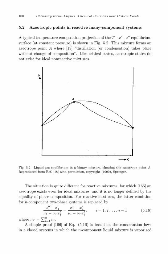
September 11, 2009 10:7 World Scientific Book - 9in x 6in General-nn
100 Chemistry versus Physics: Chemical Reactions near Critical Points
5.2 Azeotropic points in reactive many-component systems
A typical temperature-composition projection of the T−x′−x′′ equilibriumsurface (at constant pressure) is shown in Fig. 5.2. This mixture forms anazeotrope point A where [19] “distillation (or condensation) takes placewithout change of composition”. Like critical states, azeotropic states donot exist for ideal nonreactive mixtures.
Fig. 5.2 Liquid-gas equilibrium in a binary mixture, showing the azeotrope point A.Reproduced from Ref. [18] with permission, copyright (1990), Springer.
The situation is quite different for reactive mixtures, for which [166] anazeotrope exists even for ideal mixtures, and it is no longer defined by theequality of phase composition. For reactive mixtures, the latter conditionfor n-component two-phase systems is replaced by
x′′1 − x′1ν1 − νTx′1
=x′′i − x′iνi − νTx′i
; i = 1, 2, . . . , n− 1 (5.16)
where νT =∑n
i=1 νi.
A simple proof [166] of Eq. (5.16) is based on the conservation lawsin a closed systems in which the n-component liquid mixture is vaporized
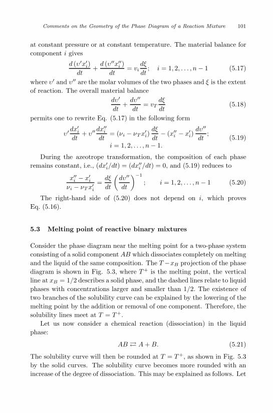
September 11, 2009 10:7 World Scientific Book - 9in x 6in General-nn
Comments on the Geometry of the Phase Diagram of a Reaction Mixture 101
at constant pressure or at constant temperature. The material balance forcomponent i gives
d (υ′x′i)dt
+d (υ′′x′′i )
dt= vi
dξ
dt; i = 1, 2, . . . , n− 1 (5.17)
where υ′ and υ′′ are the molar volumes of the two phases and ξ is the extentof reaction. The overall material balance
dυ′
dt+dυ′′
dt= vT
dξ
dt(5.18)
permits one to rewrite Eq. (5.17) in the following form
υ′dx′idt
+ υ′′dx′′idt
= (νi − νTx′i)dξ
dt− (x′′i − x′i)
dυ′′
dt;
i = 1, 2, . . . , n− 1.(5.19)
During the azeotrope transformation, the composition of each phaseremains constant, i.e., (dx′i/dt) = (dx′′i /dt) = 0, and (5.19) reduces to
x′′i − x′iνi − νTx′i
=dξ
dt
(dυ′′
dt
)−1
; i = 1, 2, . . . , n− 1 (5.20)
The right-hand side of (5.20) does not depend on i, which provesEq. (5.16).
5.3 Melting point of reactive binary mixtures
Consider the phase diagram near the melting point for a two-phase systemconsisting of a solid component AB which dissociates completely on meltingand the liquid of the same composition. The T −xB projection of the phasediagram is shown in Fig. 5.3, where T+ is the melting point, the verticalline at xB = 1/2 describes a solid phase, and the dashed lines relate to liquidphases with concentrations larger and smaller than 1/2. The existence oftwo branches of the solubility curve can be explained by the lowering of themelting point by the addition or removal of one component. Therefore, thesolubility lines meet at T = T+.
Let us now consider a chemical reaction (dissociation) in the liquidphase:
AB � A+B. (5.21)
The solubility curve will then be rounded at T = T+, as shown in Fig. 5.3by the solid curves. The solubility curve becomes more rounded with anincrease of the degree of dissociation. This may be explained as follows. Let
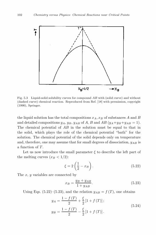
September 11, 2009 10:7 World Scientific Book - 9in x 6in General-nn
102 Chemistry versus Physics: Chemical Reactions near Critical Points
Fig. 5.3 Liquid-solid solubility curves for compound AB with (solid curve) and without(dashed curve) chemical reaction. Reproduced from Ref. [18] with permission, copyright(1990), Springer.
the liquid solution has the total compositions xA, xB of substances A and Band detailed compositions yA, yB, yAB of A, B and AB (yA+yB+yAB = 1).The chemical potential of AB in the solution must be equal to that inthe solid, which plays the role of the chemical potential “bath” for thesolution. The chemical potential of the solid depends only on temperatureand, therefore, one may assume that for small degrees of dissociation, yAB isa function of T .
Let us now introduce the small parameter ξ to describe the left part ofthe melting curves (xB < 1/2):
ξ = 2(
12− xB
). (5.22)
The x, y variables are connected by
xB =yB + yAB
1 + yAB. (5.23)
Using Eqs. (5.22)–(5.23), and the relation yAB = f (T ), one obtains
yA =1− f (T )
2+ξ
2[1 + f (T )] ;
yB =1− f (T )
2− ξ
2[1 + f (T )] .
(5.24)
September 11, 2009 10:7 World Scientific Book - 9in x 6in General-nn
Comments on the Geometry of the Phase Diagram of a Reaction Mixture 103
If dissociation is slight, than the solution is ideal. Therefore, one can writethe law of mass action for the reaction (5.21) as follows,
yAyB = K (T ) . (5.25)
Inserting (5.24) into (5.25), one can rewrite the latter in the form
ξ2 =[1− f (T )]2
[1 + f (T )]2− 4K (T )
[1 + f (T )]2≡ Q (T )2 −R (T )2 . (5.26)
At T = T+, ξ = 0, i.e., Q (T+) = R (T+) . Expanding Eq. (5.26) nearT = T+ yields
ξ2 = 2Q(T+) [(dR
dT
)−(dQ
dT
)]T=T+
(T+ − T )+ · · · . (5.27)
Equation (5.27) describes a melting line in the presence of a chemical reac-tion (solid curve in Fig. 5.3).
We now turn to the case of a nonreactive mixture. Then, K (T ) = 0 ,and the first term in the series expansion of Eq. (5.26) near T = T+ is ofsecond order,
ξ2 =(dQ
dT
)2
T=T+
(T+ − T )2 . (5.28)
In this case the melting lines (the dashed curves in Fig. 5.3) meet at a point.The reason for the difference between Eqs. (5.27) and (5.28) was ex-
plained back in 1892 [167]. If there were any appreciable dissociation of ABinto its constituents, then, in contrast to the non-dissociated solution, thesmall addition of either component will not change the equilibrium tem-perature. Therefore, the melting point is a true maximum of a solid curve[Eq. (5.27)] and not a kink [Eq. (5.28)].
Similar results are obtained from more general considerations, includ-ing the more complicated compounds AmBn [168] and the strictly regularsolution model [169] (instead of an ideal model).
Further development of these ideas has been carried out by Krichevskiiet al. [170], [171]. They considered the influence of a third componenton the thermodynamics of the three-phase equilibrium among a solid phase(compound ABm, a solvent B with a dissolved substance A), a liquid phase(solution saturated with this component and extremely dilute with respectto component C), and a gas phase (vapor of the pure solvent B with thecomponents A and C assumed to be nonvolatile).
For a non-dissociated system, the change in fugacity of the solvent B(which, for the low saturated vapor pressure, coincides with the partial
September 11, 2009 10:7 World Scientific Book - 9in x 6in General-nn
104 Chemistry versus Physics: Chemical Reactions near Critical Points
pressure) due to the addition of a small amount of C at constant pressureand temperature, is given by [172]
lnp
B,(ABC)
pB,(AB)
= −nC
nB(5.29)
where pB,(AB) and p
B,(ABC) are the partial pressures of the solvent in binaryand ternary solutions at the same temperature, and n is the number ofmoles of the components.
Let us now allow the chemical reaction (dissociation) in the solution,
ABm � A+mB. (5.30)
The chemical potential of the compound ABm in solution, which coexistswith a solid, is fixed and depends only on the temperature. The fugacity γof the nonvolatile component A can be replaced by the activity a. Therefore,the law of mass action for the reaction (5.30) can be written as
aAγmB = K (5.31)
or, in differential form,
d (ln aA) +m d ln (γB) = 0. (5.32)
Combining this equation with the Gibbs-Duhem equation [3]
nA d (ln aA) + nB d (ln aB) + nC d (ln aC) = 0 (5.33)
one obtains
d ln (γB) = −nCd (ln aC)nB −mnA
(5.34)
If the solution is very dilute with respect to C, one can replace the activityaC by the numbers of moles nC .
Integrating Eq. (5.34) yields
lnγ
B,(ABC)
γB,(AB)
= lnp
B,(ABC)
pB,(AB)
= − nC
nB,0 −mnA,0(5.35)
For the chemical reaction of the form (5.30), the difference nB −mnA
remains constant. Consequently, we replace nB and nA by the total numberof moles of the components nB,0 and nA,0 in both liquid and solid phases.
At m = 0, Eq. (5.35) reduces to Eq. (5.29). At the melting point in Fig.5.3 (drawn form = 1), where two branches of the solubility curves meet, thecompositions of the solid and liquid phases are equal, and the denominatorof Eq. (5.35) reduces to zero. Addition of component C to solution must
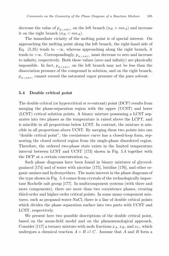
September 11, 2009 10:7 World Scientific Book - 9in x 6in General-nn
Comments on the Geometry of the Phase Diagram of a Reaction Mixture 105
decrease the value of pB,(ABC) on the left branch (nB > mnA) and increase
it on the right branch (nB < mnA).The immediate vicinity of the melting point is of special interest. On
approaching the melting point along the left branch, the right-hand side ofEq. (5.35) tends to −∞, whereas approaching along the right branch, ittends to +∞. Correspondingly, p
B,(ABC) must decrease to zero and increaseto infinity, respectively. Both these values (zero and infinity) are physicallyimpossible. In fact, p
B,(ABC) on the left branch may not be less than thedissociation pressure of the compound in solution, and on the right branch,p
B,(ABC) cannot exceed the saturated vapor pressure of the pure solvent.
5.4 Double critical point
The double critical (or hypercritical or re-entrant) point (DCP) results frommerging the phase-separation region with the upper (UCST) and lower(LCST) critical solution points. A binary mixture possessing a LCST sep-arates into two phases as the temperature is raised above the LCPT, andis miscible in all proportions below LCST. In contrast, the mixture is mis-cible in all proportions above UCST. By merging these two points into one“double critical point”, the coexistence curve has a closed-loop form, sep-arating the closed ordered region from the single-phase disordered region.Therefore, the ordered two-phase state exists in the limited temperatureinterval between LCST and UCST [173] shown in Fig. 5.4 together withthe DCP at a certain concentration x0.
Such phase diagrams have been found in binary mixtures of glycerol-guaiacol [174] and of water with nicotine [175], lutidine [176], and other or-ganic amines and hydroxyethers. The main interest in the phase diagrams ofthe type shown in Fig. 5.4 comes from crystals of the technologically impor-tant Rochelle salt group [177]. In multicomponent systems (with three andmore components), there are more than two coexistence phases, creatingthird-order and higher-order critical points. In some many-component mix-tures, such as propanol-water-NaCl, there is a line of double critical pointswhich divides the phase separation surface into two parts with UCST andLCST, respectively.
We present here two possible descriptions of the double critical point,based on the mean-field model and on the phenomenological approach.Consider [117] a ternary mixture with mole fractions xA, xB , and xC , whichundergoes a chemical reaction A + B � C. Assume that A and B form a
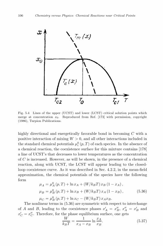
September 11, 2009 10:7 World Scientific Book - 9in x 6in General-nn
106 Chemistry versus Physics: Chemical Reactions near Critical Points
Fig. 5.4 Lines of the upper (UCST) and lower (LCST) critical solution points whichmerge at concentration x0. Reproduced from Ref. [173] with permission, copyright(1986), Turpion Publications.
highly directional and energetically favorable bond in becoming C with apositive interaction of mixing W > 0, and all other interactions included inthe standard chemical potentials µ0
i (p, T ) of each species. In the absence ofa chemical reaction, the coexistence surface for this mixture contains [178]a line of UCST’s that decreases to lower temperatures as the concentrationof C is increased. However, as will be shown, in the presence of a chemicalreaction, along with UCST, the LCST will appear leading to the closed-loop coexistence curve. As it was described in Sec. 4.2.2, in the mean-fieldapproximation, the chemical potentials of the species have the followingform
µA = µ0A (p, T ) + lnxA + (W/kBT )xB (1− xA) ,
µB = µ0B (p, T ) + lnxB + (W/kBT )xA (1− xB) ,
µC = µ0B (p, T ) + lnxC − (W/kBT )xAxB.
(5.36)
The nonlinear terms in (5.36) are symmetric with respect to interchangeof A and B, leading to the coexistence phases x′A = x′′B, x′′A = x′B andx′C = x′′C . Therefore, for the phase equilibrium surface, one gets
W
kBT=
1xA − xB
lnxA
xB. (5.37)
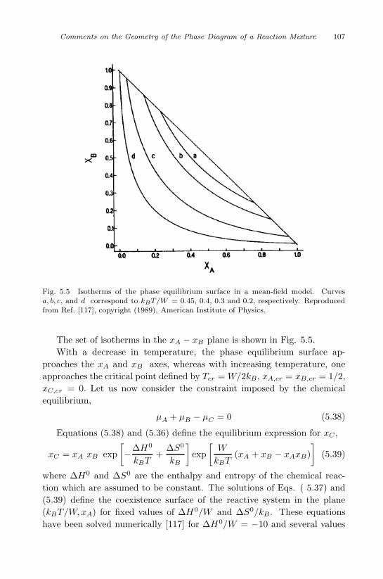
September 11, 2009 10:7 World Scientific Book - 9in x 6in General-nn
Comments on the Geometry of the Phase Diagram of a Reaction Mixture 107
Fig. 5.5 Isotherms of the phase equilibrium surface in a mean-field model. Curvesa, b, c, and d correspond to kBT/W = 0.45, 0.4, 0.3 and 0.2, respectively. Reproducedfrom Ref. [117], copyright (1989), American Institute of Physics.
The set of isotherms in the xA − xB plane is shown in Fig. 5.5.With a decrease in temperature, the phase equilibrium surface ap-
proaches the xA and xB axes, whereas with increasing temperature, oneapproaches the critical point defined by Tcr = W/2kB, xA,cr = xB,cr = 1/2,xC,cr = 0. Let us now consider the constraint imposed by the chemicalequilibrium,
µA + µB − µC = 0 (5.38)
Equations (5.38) and (5.36) define the equilibrium expression for xC ,
xC = xA xB exp[−∆H0
kBT+
∆S0
kB
]exp
[W
kBT(xA + xB − xAxB)
](5.39)
where ∆H0 and ∆S0 are the enthalpy and entropy of the chemical reac-tion which are assumed to be constant. The solutions of Eqs. ( 5.37) and(5.39) define the coexistence surface of the reactive system in the plane(kBT/W, xA) for fixed values of ∆H0/W and ∆S0/kB. These equationshave been solved numerically [117] for ∆H0/W = −10 and several values
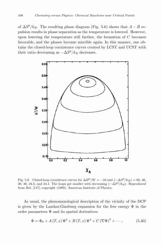
September 11, 2009 10:7 World Scientific Book - 9in x 6in General-nn
108 Chemistry versus Physics: Chemical Reactions near Critical Points
of ∆S0/kB. The resulting phase diagram (Fig. 5.6) shows that A − B re-pulsion results in phase separation as the temperature is lowered. However,upon lowering the temperature still further, the formation of C becomesfavorable, and the phases become miscible again. In this manner, one ob-tains the closed-loop coexistence curves created by LCST and UCST withtheir ratio decreasing as −∆S0/kB decreases.
Fig. 5.6 Closed-loop coexistence curves for ∆H0/W = −10 and(−∆S0/kB
)= 60, 40,
30, 26, 24.5, and 24.1. The loops get smaller with decreasing (−∆S0/kB). Reproducedfrom Ref. [117], copyright (1989), American Institute of Physics.
As usual, the phenomenological description of the vicinity of the DCPis given by the Landau-Ginzburg expansion for the free energy Φ in theorder parameters Ψ and its spatial derivatives:
Φ = Φ0 +A (T, x)Ψ2 +B (T, x)Ψ4 + C (∇Ψ)2 + · · · , (5.40)
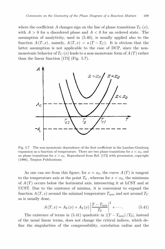
September 11, 2009 10:7 World Scientific Book - 9in x 6in General-nn
Comments on the Geometry of the Phase Diagram of a Reaction Mixture 109
where the coefficient A changes sign on the line of phase transitions TC (x),with A > 0 for a disordered phase and A < 0 for an ordered state. Theassumption of analyticity, used in (5.40), is usually applied also to thefunction A (T, x) , namely, A (T, x) = a (T − TC). It is obvious that thelatter assumption is not applicable to the case of DCP, since the non-monotonic behavior of TC (x) leads to a non-monotonic form ofA (T ) ratherthan the linear function [173] (Fig. 5.7).
Fig. 5.7 The non-monotonic dependence of the first coefficient in the Landau-Ginzburgexpansion as a function of temperature. There are two phase transitions for x < x0, andno phase transitions for x > x0. Reproduced from Ref. [173] with permission, copyright(1986), Turpion Publications.
As one can see from this figure, for x = x0, the curve A (T ) is tangentto the temperature axis at the point T0 , whereas for x < x0, the minimumof A (T ) occurs below the horizontal axis, intersecting it at LCST and atUCST. Due to the existence of minima, it is convenient to expand thefunction A (T, x) around the minimal temperature Tmin and not around TC
as is usually done,
A (T, x) = A0 (x) + A2 (x)∣∣∣∣T − Tmin
T0
∣∣∣∣2 + · · · . (5.41)
The existence of terms in (5.41) quadratic in |(T − Tmin) /T0|, insteadof the usual linear terms, does not change the critical indices, which de-fine the singularities of the compressibility, correlation radius and the
September 11, 2009 10:7 World Scientific Book - 9in x 6in General-nn
110 Chemistry versus Physics: Chemical Reactions near Critical Points
quantities related to them. However, the anomalies of the quantitiescontaining the derivatives of the coefficient A with respect to tempera-ture, decrease near the DCP. For example, the jump of the heat capacity∆C = −T∂2
(A2/2B
)/∂T 2 at LCST and UCST decreases proportional to
the square of the relative distance between these points. Indeed, a decreaseof several orders of magnitude in the anomalies of the heat capacity wasfound in all systems with the DCP. However, there are some discrepanciesbetween the theory and experiment [173] which makes specially interest-ing the microscopic description of the DCP and the close-loop coexistencecurves which have been carried out in the context of lattice-gas [179] anddecorated-lattice-gas [96] models.
It should be noted that the anomaly of the kinetic coefficients are alsodifferent from the usual critical point. For example, near DCP, the mea-surements of the shear viscosity of ternary mixtures of 3-methylpyridine,water and heavy water as a function of temperature show [180] that nearDCP, the exponent describing the power-law divergence in temperature ofthe viscosity nearly doubles as the concentration approaches the double-critical-point concentration. There are also experimental data describinglight scattering and sound propagation near the DCT [181]. However, weare unaware of any experiments of chemical reactions near DCP, which areof special interest.
September 11, 2009 10:7 World Scientific Book - 9in x 6in General-nn
Chapter 6
Sound Propagation and LightScattering in Chemically
Reactive Systems
6.1 Ultrasound attenuation in near-critical reactivemixtures
The idea of using the attenuation of sound to study the rate of dissociationof the reaction N2O4 � 2NO2 was proposed in 1920 by Albert Einstein[182]. The total attenuation per wavelength αλ near the critical point canbe written as
αλ = (αλ)cr + (αλ)chem , (6.1)
neglecting the small background contribution due to viscosity and thermalconductivity. Equation (6.1) contains the assumption of the additive contri-butions of (αλ)cr and (αλ)chem, which come from the critical fluctuationsand chemical reaction, respectively. The assumption of independence ofthese two contributions is based on the following picture [183]: the reactiontakes the system from equilibrium to the steady state, which afterwardswill relax to the initial equilibrium state with characteristic relaxation timeτ chem. The latter defines the sound attenuation due to a chemical reaction
(αλ)chem = A0ωτchem
1 + (ωτchem)2(6.2)
which depends on the nearness to the critical point, since τchem is propor-tional to the equilibrium derivative of the extent of reaction ξ with respectto the affinity A, τchem ∼ (∂ξ/∂A)eq [36].
The calculation of the critical contribution to the sound attenuation,expressed by the (αλ)cr term in Eq. (2.77 ), has been performed [184].This theory is based on an assumption going back to Laplace [185], whocorrected Newton calculation showing that the sound velocity in air shouldbe calculated using the adiabatic rather than the isothermal compressibil-ity. In line with this comment, it was assumed [184] that the change of
111
September 11, 2009 10:7 World Scientific Book - 9in x 6in General-nn
112 Chemistry versus Physics: Chemical Reactions near Critical Points
pressure caused by the propagating sound, produces a shift in the criticaltemperature, but not in the critical concentration. Neglecting the changesin concentration, we are left with two thermodynamic variables p and T ,or p and τ ≡ T − TC (p), where TC (p) is the pressure-temperature criticalline. Simple thermodynamic analysis shows [184] that the sound veloc-ity u remains constant at the critical point, u (T = TC) ≡ uC , with smallcorrections ∆u near the critical point,
u ≡ uC + ∆u = uC +g2u3
C
2TCCp(6.3)
where g = TC (∂S/∂p)λ-line V−1C is a dimensionless constant, and Cp is the
specific heat. The above analysis has been performed at non-zero frequencyω for an input pressure signal with time dependence exp (−iωt). Therefore,Eq. (6.3) determines the complex sound velocity u (ω) as a function of thecomplex specific heat Cp (ω). Dynamic scaling theory has been used to de-termine the frequency dependence of Cp (ω) from the known temperaturedependence of the thermodynamic heat capacity Cp. The function Cp (ω)can be divided into the noncritical frequency-independent background com-ponent C1 and the critical part C (ω), where Cp = C1 + C (0). The low-frequency expansion of Cp (ω) gives
C (ω) ≈ C (0) + ωC � (0) = C (0) (1 + iωτ ) (6.4)
where τ = −iC′1 (0) /C (0) is an effective mean relaxation time. Upon in-
serting (6.4) into (6.3) and assuming ωτ << 1, one obtains for the negativeimaginary part of the critical velocity Im (uC) (the sound attenuation perwavelength αcrλ),
αcrλ = C (0)u3
C
2TC
(g
Cp
)2
ωτ. (6.5)
The critical part of the specific heat C (0) , induced by concentrationfluctuations, has the following thermodynamic temperature dependence
C (0) ≈ t−α0 (6.6)
where α0 is the critical index and t = ∆T/TC = (T − TC) /TC is the re-duced temperature. The relaxation rate of concentration fluctuations ofwavenumber k is k2D, where the critical diffusion coefficient is D (ξ) =kBTC/6πηξ with ξ ≈ t−ν and η ≈ t−z0 . Therefore, the characteristic relax-ation time for the fluid is
γ (t) = 2Dξ−2 = γ0 (∆T )νz0 (6.7)
September 11, 2009 10:7 World Scientific Book - 9in x 6in General-nn
Sound Propagation and Light Scattering in Chemically Reactive Systems 113
where γ0 is constant. Equation (6.7) enables us to eliminate t in favour ofγ as the variable that indicates how close the system is to the critical point,
C (γ, ω = 0) = B
(γ0
γ
)α0/νz0
. (6.8)
According to the dynamic-scaling requirement [186], the dependence ofEq. (6.8) on γ disappears when, for γ < ω, γ is replaced by −iω so thatthe frequency-dependent specific heat at the critical point is
C (γ = 0, ω) = B
(γ0
−iω)α0/νz0
= B exp(iπα0
νz0
)(γ0
ω
)α0/νz0
. (6.9)
Replacing C (0) in Eq. (6.5) by the imaginary part of C (γ = 0, ω) , andusing α0 << νz0, one gets finally
αcrλ π2α0g2u2
CB
2TCC2p (Tc)
( γ0
2π
)α0/νz0
f−α0/νz0 (6.10)
where f = ω/2π is the frequency. Multiplying Eq. (6.10) by (uCf)−1
predicts a linear proportionality between αcrf−2 and f−1−α0/νz0 . Pre-
cisely this dependence had been observed in the measurements [184] ofthe sound attenuation in 3-methylpentane-nitroethane at various frequen-cies ranging from 16.5 to 165 MHz. Agreement between theory and ex-periment was also found for polypropylene-glycol and polyethylene-glycolmixtures [188], iso-butoxyethanol-water system [189], ethanol-dodecaneand methanol-cyclohexane mixtures [190], cyclohexane-nitroethane[191],methanol-hexane [192], and triethylamine-water, methanol-cyclohexane[193].
6.2 Hydrodynamic analysis of the dispersion relation forsound waves
Sound waves are oscillating movements of small amplitude, which give riseto small perturbations in the system. Therefore, one can use the linearizedhydrodynamic equations for the analysis of the sound velocity and attenua-tion coefficient in fluids. The linearized system of hydrodynamic equationsfor reactive systems was obtained in Chapter 2. We will here use the fol-lowing simplified version of these equations [194]
September 11, 2009 10:7 World Scientific Book - 9in x 6in General-nn
114 Chemistry versus Physics: Chemical Reactions near Critical Points
∂ρ
∂t= −ρ0div (v) (6.11)
ρ0
∂v
∂t= −grad (p) + η∇2v
+(η
3+ ζ)grad (div (v)) + ρ0L1grad (A) (6.12)
∂ξ
∂t= −L0A− L1div (v) (6.13)
A =(∂A
∂ρ
)ξ,S
ρ+(∂A
∂ξ
)ρ,S
ξ +(∂A
∂S
)ξ,ρ
S (6.14)
p =(∂p
∂ρ
)ξ,S
ρ+(∂p
∂ξ
)ρ,S
ξ +(∂p
∂S
)ξ,ρ
S (6.15)
T =(∂T
∂ρ
)ξ,S
ρ+(∂T
∂ξ
)ρ,S
ξ +(∂T
∂S
)ξ,ρ
S. (6.16)
In contrast to Eqs. (2.61)–(2.64), the independent variables in the aboveequations are the velocity v, the deviations from equilibrium values of en-tropy s, density ρ and extent of reaction ξ. Kinetic coefficients are takinginto account only in the Navier-Stokes equation (6.12).
To derive the dispersion law, we take the Fourier transform of the hy-drodynamic variables
X (K, ω) =∫d3r
∫dtx (r, t) exp (iωt− iKr) . (6.17)
The wave vector K is written K = k + iγ, where k is the propagationvector and γ is the attenuation coefficient.
After some additional simplifications [194], Eqs. (6.11)–(6.16) yield thefollowing expressions for k and γ
k =ω
C; γ =
ω2
2ρ0
G
C3(6.18)
where
C2 ≡ − 1ρ20
( ∂p∂υ
)ξ,S
+
(∂p∂ξ
)v,S
(∂ξ∂υ
)A,S
1 + ω2τ2
+ 2ρ0L1
(∂p
∂ξ
)υ,S
ω2τ2
1 + ω2τ2
](6.19)
September 11, 2009 10:7 World Scientific Book - 9in x 6in General-nn
Sound Propagation and Light Scattering in Chemically Reactive Systems 115
G ≡(∂p
∂ξ
)υ,S
[(∂ξ
∂υ
)A,s
τ
ρ0 (1 + ω2τ2)
+2τL1
1 + ω2τ2
]+
4η3
+ ζ (6.20)
and the relaxation time τ is given by
τ ≡[L0
(∂A
∂ξ
)υ,S
]−1
. (6.21)
Some limit cases of these general equations has been considered [194].This theory contains visco-reactive cross coefficients L1, which link the
chemical reaction to the momentum flow, which is important for a weakelectrolyte solution [194]. Now let us turn to the slightly different hydro-dynamic approach, which allows us to consider the vicinity of the criticalpoints without the L1 terms [195]. Starting from the same hydrodynamicequations obtained in Chapter 2, we replace them by the statistically in-dependent variables as it was done there. However, instead of variables ξ,p, div (v) and φ = Cp,xT/T0 − αT p/ρ0, we use the set ξ, p, div (v) andS1 = S − (∂S/∂ξ) ξ. The hydrodynamic equations (2.91)–(2.94) may thenbe rearranged to give
∂ρ
∂t= −ρ0div (v) (6.22)
ρ0
∂div (v)∂t
= −∇2p+(
43η + ζ
)∇2div (v) (6.23)
∂ξ
∂t= D
[∇2ξ +
kT
T0∇2T +
kp
p0∇2p
]
+1τT,p
[ξ −
(∂ξ
∂T
)p,A
T −(∂ξ
∂p
)T,A
p
](6.24)
∂S1
∂t=
λ
ρ0T0∇2T +D
kT
T0
(∂A
∂ξ
)T,p
[∇2ξ +
kp
p0∇2p
]
+D
(∂S
∂ξ
)p,T
[∇2ξ +
kT
T0∇2T +
kp
p0∇2p
](6.25)
September 11, 2009 10:7 World Scientific Book - 9in x 6in General-nn
116 Chemistry versus Physics: Chemical Reactions near Critical Points
where τT,p =[L (∂A/∂ξ)T,p
]−1
is the relaxation time, and all other nota-tion has been explained in Chapter 2.
Since only the fluctuations of concentration and entropy become anoma-lously large near the critical point, we may use the simplified macroscopicequations (6.24)–(6.25) in which the pressure is kept constant. Introduc-ing both normalized and statistically independent spatial Fourier transformvariables, one obtains
β1 (k, t) =(
ρ0
kBυCp,ξ
)1/2
S1 (k, t) ,
β2 (k, t) = ρ0
[ (∂A/∂ξ)T.p
kBTυ
]1/2
ξ (K, t) .
(6.26)
It is easy to show [195] that
d
dt
(β1 (K, t)β2 (K, t)
)= M
(β1 (K, t)β2 (K, t)
)(6.27)
where the 2× 2 matrix M is given by
M =
λK2
ρ0Cp,ξ
+γT
τT,p, kTD
√( ∂A
∂ξ )T.p
TCp,ξK2 − γ
1/2T
τT,p
kTD
√( ∂A
∂ξ )T.p
TCp,ξK2 − γ
1/2T
τT,p, DK2 + τ−1
T,p
(6.28)
and
γT ≡Cp,A − Cp,ξ
Cp,ξ. (6.29)
The non-diagonal elements of the matrix M are very small and may beneglected if the propagation number K satisfies the inequality
K >
Cp,A − Cp,ξ(λρ0−DCp,ξ
)τT,p
1/2
. (6.30)
Numerical estimates indicate that (6.30) is satisfied for K > 104 cm −1.The variables β1 (k, t) and β2 (k, t) are then effectively decoupled, and
〈ξ (K, t) ξ (−K, t)〉 = exp[−(DK2 + τ−1
T,p
)t]〈ξ (K) ξ (−K)〉 . (6.31)
The mode-coupling method has been used [102] in the analysis of thepropagation of sound in a non-reactive binary mixture near the critical
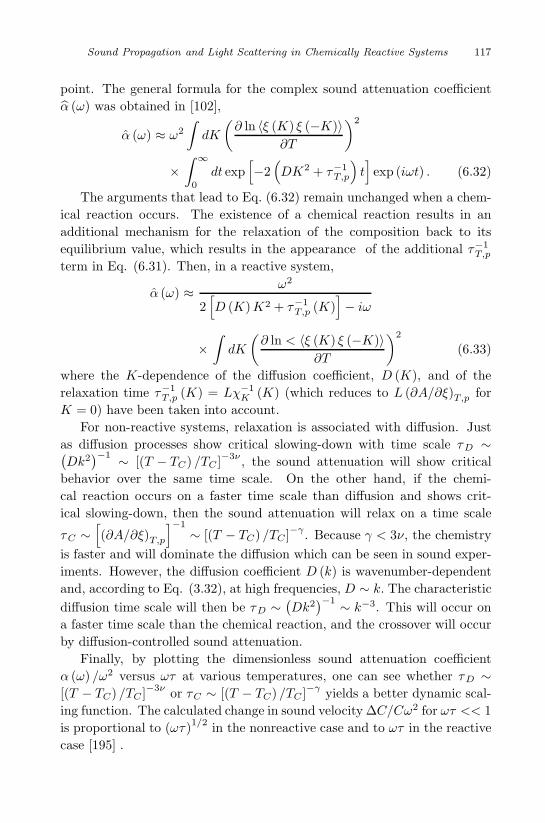
September 11, 2009 10:7 World Scientific Book - 9in x 6in General-nn
Sound Propagation and Light Scattering in Chemically Reactive Systems 117
point. The general formula for the complex sound attenuation coefficientα (ω) was obtained in [102],
α (ω) ≈ ω2
∫dK
(∂ ln 〈ξ (K) ξ (−K)〉
∂T
)2
×∫ ∞
0
dt exp[−2(DK2 + τ−1
T,p
)t]exp (iωt) . (6.32)
The arguments that lead to Eq. (6.32) remain unchanged when a chem-ical reaction occurs. The existence of a chemical reaction results in anadditional mechanism for the relaxation of the composition back to itsequilibrium value, which results in the appearance of the additional τ−1
T,p
term in Eq. (6.31). Then, in a reactive system,
α (ω) ≈ ω2
2[D (K)K2 + τ−1
T,p (K)]− iω
×∫dK
(∂ ln < 〈ξ (K) ξ (−K)〉
∂T
)2
(6.33)
where the K-dependence of the diffusion coefficient, D (K), and of therelaxation time τ−1
T,p (K) = Lχ−1K (K) (which reduces to L (∂A/∂ξ)T,p for
K = 0) have been taken into account.For non-reactive systems, relaxation is associated with diffusion. Just
as diffusion processes show critical slowing-down with time scale τD ∼(Dk2
)−1 ∼ [(T − TC) /TC ]−3ν , the sound attenuation will show criticalbehavior over the same time scale. On the other hand, if the chemi-cal reaction occurs on a faster time scale than diffusion and shows crit-ical slowing-down, then the sound attenuation will relax on a time scale
τC ∼[(∂A/∂ξ)T,p
]−1
∼ [(T − TC) /TC ]−γ . Because γ < 3ν, the chemistryis faster and will dominate the diffusion which can be seen in sound exper-iments. However, the diffusion coefficient D (k) is wavenumber-dependentand, according to Eq. (3.32), at high frequencies, D ∼ k. The characteristicdiffusion time scale will then be τD ∼
(Dk2
)−1 ∼ k−3. This will occur ona faster time scale than the chemical reaction, and the crossover will occurby diffusion-controlled sound attenuation.
Finally, by plotting the dimensionless sound attenuation coefficientα (ω) /ω2 versus ωτ at various temperatures, one can see whether τD ∼[(T − TC) /TC ]−3ν or τC ∼ [(T − TC) /TC ]−γ yields a better dynamic scal-ing function. The calculated change in sound velocity ∆C/Cω2 for ωτ << 1is proportional to (ωτ)1/2 in the nonreactive case and to ωτ in the reactivecase [195] .
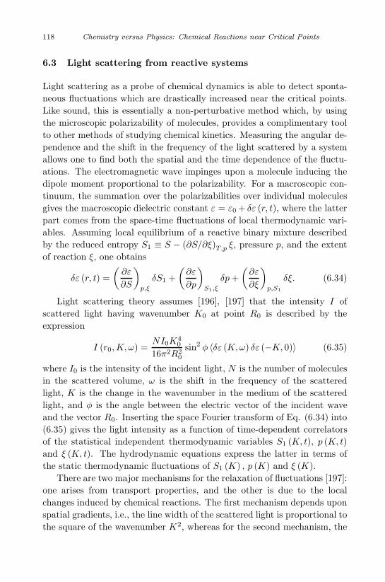
September 11, 2009 10:7 World Scientific Book - 9in x 6in General-nn
118 Chemistry versus Physics: Chemical Reactions near Critical Points
6.3 Light scattering from reactive systems
Light scattering as a probe of chemical dynamics is able to detect sponta-neous fluctuations which are drastically increased near the critical points.Like sound, this is essentially a non-perturbative method which, by usingthe microscopic polarizability of molecules, provides a complimentary toolto other methods of studying chemical kinetics. Measuring the angular de-pendence and the shift in the frequency of the light scattered by a systemallows one to find both the spatial and the time dependence of the fluctu-ations. The electromagnetic wave impinges upon a molecule inducing thedipole moment proportional to the polarizability. For a macroscopic con-tinuum, the summation over the polarizabilities over individual moleculesgives the macroscopic dielectric constant ε = ε0 + δε (r, t), where the latterpart comes from the space-time fluctuations of local thermodynamic vari-ables. Assuming local equilibrium of a reactive binary mixture describedby the reduced entropy S1 ≡ S − (∂S/∂ξ)T,p ξ, pressure p, and the extentof reaction ξ, one obtains
δε (r, t) =(∂ε
∂S
)p,ξ
δS1 +(∂ε
∂p
)S1,ξ
δp+(∂ε
∂ξ
)p,S1
δξ. (6.34)
Light scattering theory assumes [196], [197] that the intensity I ofscattered light having wavenumber K0 at point R0 is described by theexpression
I (r0,K, ω) =NI0K
40
16π2R20
sin2 φ 〈δε (K,ω) δε (−K, 0)〉 (6.35)
where I0 is the intensity of the incident light, N is the number of moleculesin the scattered volume, ω is the shift in the frequency of the scatteredlight, K is the change in the wavenumber in the medium of the scatteredlight, and φ is the angle between the electric vector of the incident waveand the vector R0. Inserting the space Fourier transform of Eq. (6.34) into(6.35) gives the light intensity as a function of time-dependent correlatorsof the statistical independent thermodynamic variables S1 (K, t), p (K, t)and ξ (K, t). The hydrodynamic equations express the latter in terms ofthe static thermodynamic fluctuations of S1 (K) , p (K) and ξ (K).
There are two major mechanisms for the relaxation of fluctuations [197]:one arises from transport properties, and the other is due to the localchanges induced by chemical reactions. The first mechanism depends uponspatial gradients, i.e., the line width of the scattered light is proportional tothe square of the wavenumber K2, whereas for the second mechanism, the
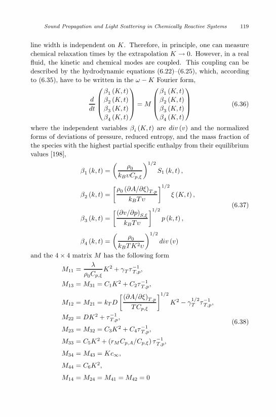
September 11, 2009 10:7 World Scientific Book - 9in x 6in General-nn
Sound Propagation and Light Scattering in Chemically Reactive Systems 119
line width is independent on K. Therefore, in principle, one can measurechemical relaxation times by the extrapolation K → 0. However, in a realfluid, the kinetic and chemical modes are coupled. This coupling can bedescribed by the hydrodynamic equations (6.22)–(6.25), which, accordingto (6.35), have to be written in the ω −K Fourier form,
d
dt
β1 (K, t)β2 (K, t)β3 (K, t)β4 (K, t)
= M
β1 (K, t)β2 (K, t)β3 (K, t)β4 (K, t)
(6.36)
where the independent variables βi (K, t) are div (v) and the normalizedforms of deviations of pressure, reduced entropy, and the mass fraction ofthe species with the highest partial specific enthalpy from their equilibriumvalues [198],
β1 (k, t) =(
ρ0
kBυCp,ξ
)1/2
S1 (k, t) ,
β2 (k, t) =[ρ0 (∂A/∂ξ)T.p
kBTυ
]1/2
ξ (K, t) ,
β3 (k, t) =[ (∂v/∂p)S,ξ
kBTυ
]1/2
p (k, t) ,
β4 (k, t) =(
ρ0
kBTK2υ
)1/2
div (v)
(6.37)
and the 4× 4 matrix M has the following form
M11 =λ
ρ0Cp,ξK2 + γT τ
−1T,p,
M13 = M31 = C1K2 + C2τ
−1T,p,
M12 = M21 = kTD
[ (∂A/∂ξ)T.p
TCp,ξ
]1/2
K2 − γ1/2T τ−1
T,p,
M22 = DK2 + τ−1T,p,
M23 = M32 = C3K2 + C4τ
−1T,p,
M33 = C5K2 + (rMCp,A/Cp,ξ) τ−1
T,p,
M34 = M43 = Kc∞,
M44 = C6K2,
M14 = M24 = M41 = M42 = 0
(6.38)
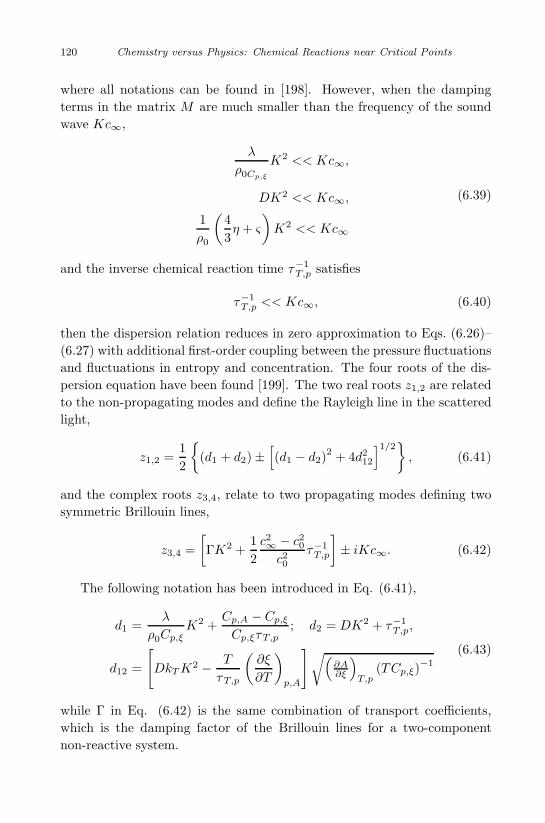
September 11, 2009 10:7 World Scientific Book - 9in x 6in General-nn
120 Chemistry versus Physics: Chemical Reactions near Critical Points
where all notations can be found in [198]. However, when the dampingterms in the matrix M are much smaller than the frequency of the soundwave Kc∞,
λ
ρ0Cp,ξ
K2 << Kc∞,
DK2 << Kc∞,
1ρ0
(43η + ς
)K2 << Kc∞
(6.39)
and the inverse chemical reaction time τ−1T,p satisfies
τ−1T,p << Kc∞, (6.40)
then the dispersion relation reduces in zero approximation to Eqs. (6.26)–(6.27) with additional first-order coupling between the pressure fluctuationsand fluctuations in entropy and concentration. The four roots of the dis-persion equation have been found [199]. The two real roots z1,2 are relatedto the non-propagating modes and define the Rayleigh line in the scatteredlight,
z1,2 =12
{(d1 + d2)±
[(d1 − d2)
2 + 4d212
]1/2}, (6.41)
and the complex roots z3,4, relate to two propagating modes defining twosymmetric Brillouin lines,
z3,4 =[ΓK2 +
12c2∞ − c20c20
τ−1T,p
]± iKc∞. (6.42)
The following notation has been introduced in Eq. (6.41),
d1 =λ
ρ0Cp,ξK2 +
Cp,A − Cp,ξ
Cp,ξτT,p; d2 = DK2 + τ−1
T,p,
d12 =
[DkTK
2 − T
τT,p
(∂ξ
∂T
)p,A
]√(∂A∂ξ
)T,p
(TCp,ξ)−1
(6.43)
while Γ in Eq. (6.42) is the same combination of transport coefficients,which is the damping factor of the Brillouin lines for a two-componentnon-reactive system.
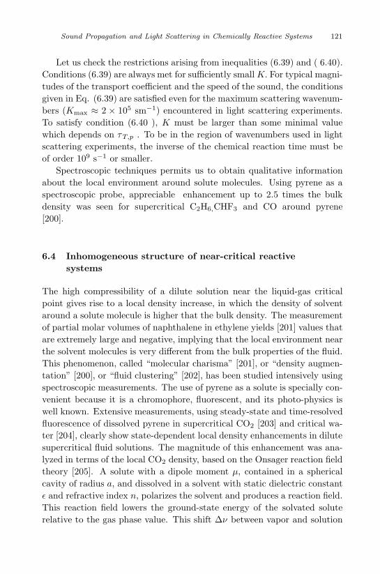
September 11, 2009 10:7 World Scientific Book - 9in x 6in General-nn
Sound Propagation and Light Scattering in Chemically Reactive Systems 121
Let us check the restrictions arising from inequalities (6.39) and ( 6.40).Conditions (6.39) are always met for sufficiently smallK. For typical magni-tudes of the transport coefficient and the speed of the sound, the conditionsgiven in Eq. (6.39) are satisfied even for the maximum scattering wavenum-bers (Kmax ≈ 2 × 10⁵ sm−1) encountered in light scattering experiments.To satisfy condition (6.40 ), K must be larger than some minimal valuewhich depends on τT,p . To be in the region of wavenumbers used in lightscattering experiments, the inverse of the chemical reaction time must beof order 109 s−1 or smaller.
Spectroscopic techniques permits us to obtain qualitative informationabout the local environment around solute molecules. Using pyrene as aspectroscopic probe, appreciable enhancement up to 2.5 times the bulkdensity was seen for supercritical C2H6,CHF3 and CO around pyrene[200].
6.4 Inhomogeneous structure of near-critical reactivesystems
The high compressibility of a dilute solution near the liquid-gas criticalpoint gives rise to a local density increase, in which the density of solventaround a solute molecule is higher that the bulk density. The measurementof partial molar volumes of naphthalene in ethylene yields [201] values thatare extremely large and negative, implying that the local environment nearthe solvent molecules is very different from the bulk properties of the fluid.This phenomenon, called “molecular charisma” [201], or “density augmen-tation” [200], or “fluid clustering” [202], has been studied intensively usingspectroscopic measurements. The use of pyrene as a solute is specially con-venient because it is a chromophore, fluorescent, and its photo-physics iswell known. Extensive measurements, using steady-state and time-resolvedfluorescence of dissolved pyrene in supercritical CO2 [203] and critical wa-ter [204], clearly show state-dependent local density enhancements in dilutesupercritical fluid solutions. The magnitude of this enhancement was ana-lyzed in terms of the local CO2 density, based on the Onsager reaction fieldtheory [205]. A solute with a dipole moment µ, contained in a sphericalcavity of radius a, and dissolved in a solvent with static dielectric constantε and refractive index n, polarizes the solvent and produces a reaction field.This reaction field lowers the ground-state energy of the solvated soluterelative to the gas phase value. This shift ∆ν between vapor and solution
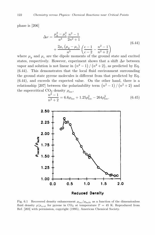
September 11, 2009 10:7 World Scientific Book - 9in x 6in General-nn
122 Chemistry versus Physics: Chemical Reactions near Critical Points
phase is [206]
∆ν =µ2
g − µ2c
a3
n2 − 12n2 + 1
+2µc
(µg − µc
)a3
(ε− 1ε− 2
− n2 − 1n2 + 2
) (6.44)
where µg and µc are the dipole moments of the ground state and excitedstates, respectively. However, experiment shows that a shift ∆ν betweenvapor and solution is not linear in
(n2 − 1
)/(n2 + 2
), as predicted by Eq.
(6.44). This demonstrates that the local fluid environment surroundingthe ground state pyrene molecules is different from that predicted by Eq.(6.44), and exceeds the expected value. On the other hand, there is arelationship [207] between the polarizability term
(n2 − 1
)/(n2 + 2
)and
the supercritical CO2 density ρloc,n2 − 1n2 + 2
= 6.6ρloc + 1.25ρ2loc − 264ρ3
loc. (6.45)
Fig. 6.1 Recovered density enhancement ρloc/ρbulk as a function of the dimensionlessfluid density ρ/ρcrit for pyrene in CO2 at temperature T = 45 K. Reproduced fromRef. [203] with permission, copyright (1995), American Chemical Society.
September 11, 2009 10:7 World Scientific Book - 9in x 6in General-nn
Sound Propagation and Light Scattering in Chemically Reactive Systems 123
Equations (6.44) and (6.45) were used [203] to find the spectral shift ∆νas a function of bulk density ρbulk. The experimental spectral shift ∆ν isused to compute a local polarizability term in Eq. (6.44), which determines[203] the local density ρloc from Eq. (6.45). In this manner, the localdensity augmentation ρloc/ρbulk was found as a function of the reduceddensity ρ/ρcrit of CO2, as shown in Fig. 6.1, which displays a local densityaugmentation up to 170 at about half the critical density. In addition tothis local density enhancement, connected with the ground state of pyrenemolecules, similar experiments have been performed for the pyrene excitedstate. The latter turned out to be 1.5 times greater than in the groundstate, due to the increased electrostatic interaction between the excitedstate of pyrene and CO2. All these results do not depend on the pyreneconcentration, indicating that pyrene molecules are solvated individuallyin CO2.
The same increase of the solvent density around a solute molecule com-pared with the corresponded bulk density has been obtained [208] using(N,N-dimethylamino) benzonitrile as a probe instead of pyrene. Additionalverification of the inhomogeneity of a near-critical reactive system has beenobtained by indirect measurements combined with thermodynamic calcu-lations [209], [210]. Finally, the same result follows from numerical simula-tions based on the Lennard-Jones potential [211] and the theory of integralequations [212].
September 11, 2009 10:7 World Scientific Book - 9in x 6in General-nn
Chapter 7
Conclusions
The main body of this book consists of a detailed discussion of the inter-connection between “physical” critical phenomena and chemical reactions.Although these two phenomena appear to be quite different, deep analysisshows [22], [21] that the instability of different nonequilibrium phenomena(hydrodynamic and chemical instabilities, laser transitions, among others)show an intimate connection with equilibrium phase transitions and crit-ical phenomena. Indeed, both are characterized by the enhancement offluctuations, long-range order and critical slowing-down. Examples of thisconnection include the relation which has been established [213] betweenthe laser threshold and the critical point of a second-order phase transi-tion, and the analogy between phase transitions of the first and secondorder and hard and soft transitions of chemical reactions. The theory ofcritical phenomena, which is supported experimentally with a precision offew decimal places, dates from the 1960’s and 1970’s. It is not surprisingthat the methods used in this theory (renormalization group, mode-modecoupling, etc) have been successfully employed in modern chemistry.
Of three branches of modern physics — theory, experiment and simu-lation — we mostly used the first in the phenomenological analysis, withreferences to experimental work given in appropriate places. Many refer-ences to numerical methods are given in review articles, such as [165], whichdescribe numerical methods of phase equilibria in reactive systems.
A near-critical fluid has some of the advantages of both a liquid anda gas: high density ensures high dissolving power which is accompaniedby high diffusivity of solutes and low viscosity facilitates mass transport.In addition, high compressibility allows the tuning of the density anddissolving power by small changes in pressure. That is the reason whychemical reactions near the critical point are in such wide use in modern
125
September 11, 2009 10:7 World Scientific Book - 9in x 6in General-nn
126 Chemistry versus Physics: Chemical Reactions near Critical Points
science and technology. Many applications can be found in review arti-cles ([156], [165]). We may mention applications in chemistry (supercriticalextraction [145]), metallurgy (the recovery of metals from coal ash [214],phase diagrams in alloy systems [215]), geochemistry (distribution and ac-tivity of species in aqueous solutions [216], solubility of minerals in brinesolutions [217]), geology (equilibria between aqueous and mineral phases[218], mineral equilibria [219]), food industry (extraction of caffeine fromcoffee beans [220] and oil from corn, sunflower and peanuts [221]), and thepharmaceutical industry (extraction of vitamin E from soybean oil and itspurification [222]).
This subject still attracts great interest, and it is very likely that manynew applications will be found in the future.
September 11, 2009 10:7 World Scientific Book - 9in x 6in General-nn
Bibliography
[1] H. G. Harris and J. M. Praushnitz, Ind. Eng. Chem. Found. 8, 180, 1969.[2] M. Gitterman, Phys. Stat. Sol. 59, 295, 1980.[3] I. Prigogine and R. Defay, Chemical Thermodynamics, Longmans Green,
New York, 1954[4] L. D. Landau and E. M. Lifshitz, Statistical Physics, Pergamon, London,
1958; Fluid Dynamics, Pergamon, London, 1987.[5] A. A. Galkin and V. V. Lunin, Russian Chem. Rev. 74, 21, 2005.[6] S. N. V. K. Aki and M. A. Abraham, Envir. Prog. 17, 246, 1998.[7] S. N. V. K. Aki and M. A. Abraham, Chem. Eng. Sci. 54, 3533, 1999.[8] A. Kruse and H. Vogel, Chem. Eng. Technol. 31, 23, 2008.[9] A. M. N. da Ponte, J. Supercrit. Fluids 47, 344, 2009.
[10] M. Gitterman, Rev. Mod. Phys. 50, 85, 1978.[11] G. Arcovito, C. Falocci, M. Riberty, and L. Mistura, Phys. Rev. Lett. 22,
1040, 1969.[12] H. E. Stanley, Introduction to Phase Transitions and Critical Phenomena,
Oxford University Press, 1993.[13] V. L. Ginzburg, Sov. Phys. - Solid State 2, 1824, 1960[14] D. Yu. Ivanov, Doklady Physics 47, 267, 2002[15] D. Yu. Ivanov, L. A. Makarevich, and O. N. Sokolova, JETP Letters 20,
121, 1974.[16] W. Wagner, N. Kurzeja, and B. Pieperbeck, Fluid Phase Equilibria 79,
151, 1992.[17] L. A. Makarevich, O. N. Sokolova, and A. M. Rozen, Sov. Phys. - JETP
40, 305, 1974.[18] M. Gitterman, J. Stat. Phys. 58, 707, 1990.[19] J. S. Rowlinson and F. I. Swinton, Liquids and Liquid Mixtures, Butter-
worth, London, 1982.[20] G. M. Schneider, Adv. Chem. Phys. 17, 1, 1970.[21] A. Nitzan, Phys. Rev. A 17, 1513, 1978.[22] A. Nitzan, P. Ortoleva, J. Deutch, and J. Ross, J. Chem. Phys. 60, 1056,
1974.[23] I. Matheson, D. F. Walls, and C. W. Gardiner, J. Stat. Phys. 12, 21, 1975.
127
September 11, 2009 10:7 World Scientific Book - 9in x 6in General-nn
128 Chemistry versus Physics: Chemical Reactions near Critical Points
[24] A. S. Mikhailov, Phys. Lett. A 73, 143, 1979; Z. Phys. B 41, 277, 1981.[25] W. Horsthemke and R. Levever, Noise-induced Transitions, Springer,
Berlin, 1984.[26] D. G. Peck, A. J. Mehta, and K. P. Johnston, J. Phys. Chem. 93, 4297,
1998.[27] B. Lin and A. Akgerman, Ind. Eng. Chem. Res. 40, 1113, 2001.[28] H. Li, B. Han, J. Liu,.L. Gao, Z. Hou, T. Jiang, Z. Liu, X. Zhang, and J.
He, Chemistry- Eur. J. 8, 5593, 2002.[29] J. Quin, M. T. Timko, A. J. Allen, C. J. Russel, B. Winnik, B. Buckley, J.
I. Steinfeld, and J. W. Tester, J. Am. Chem. Soc. 126, 5465, 2004.[30] B. Wang, B. Han, T. Jiang, Z. Zhang, Y. Xie, W. Li, and W. Wu, J. Phys.
Chem. B 109, 24203, 2005.[31] T. Nishikawa, Y. Inoue, M. Sato, Y. Iwai, and Y. Arai, AIChE J. 44, 1706,
1998.[32] S. Glasstone, K. J. Laidler, and H. Eyring, The Theory of Rate Processes,
1st ed, McGraw-Hill, New York, 1941.[33] C. A. Eckert, D. H. Ziger, K. P. Johnston, and S. J. Kim, J. Phys. Chem.
90, 2738, 1986.[34] C. Muller, A. Steiger, and F. Becker, Thermochim. Acta 151, 131, 1989.[35] L. Van Hove, Phys. Rev. 95, 1374, 1954.[36] I. Procaccia and M. Gitterman, Phys. Rev. Lett. 46, 1163, 1981; Phys.
Rev. A 25, 1137, 1982.[37] A. Z. Patashinskii, V. L. Pokrovskii, and M. V. Feigel’man, Sov. Phys. -
JETP 55, 851, 1982.[38] R. G. Griffiths and J. C. Wheeler, Phys. Rev. A 2, 1047, 1970.[39] M. E. Paulaitis and G. C. Alexander, Pure Appl. Chem. 59, 61, 1987.[40] S. T. Milner and P. C. Martin, Phys. Rev. A 33, 1996, 1986.[41] A. Onuki and R. A. Ferrell, Physica A 164, 245, 1989; B. Zappoli, D.
Bailly, Y. Garrabos, R. Le Neindre, P. Guenoun, and D. Beysens, Phys.Rev. A 41, 2264, 1990; H. I Boukari, J. N. Shaumeyer, M. E. Briggs, andR. W. Gammon, Phys. Rev. A 41, 2260, 1990.
[42] R. P. Behringer, A. Onuki, and H. Meyer, J. Low Temp. Phys. 81, 71,1990; H. Meyer and F. Zhong, Compt. Rend. Mecanique 332, 327, 2004.
[43] B. Zappoli and P. Carles, Acta Astron. 38, 39, 1996.[44] Yu. I. Dakhnovskii, A. A. Ovchinnikov, and V. A. Benderskii, Chem. Phys.
66, 93, 1982.[45] M. Sato, Y. Ikushima, K. Hatekada, and T. Ikeshoji, Int. J. Chem. Reactor
Eng. 3, A15, 2005.[46] C. E. Bunker and Ya-Ping-Sun, J. Am. Chem. Soc. 117, 10865, 1995.[47] I. Raspo, S. Meradji, and B. Zappoli, Chem. Eng. Sci. 62, 4182, 2007.[48] S.-T. Chung, H.-C. Huang, S.-J. Pan, W.-T. Tsai, P.-Y. Lee, C.-H. Yang,
and M.-B. Wu, Corrosion Science 50, 2614, 2008.[49] M. Gitterman, Physica A 386, 1, 2007.[50] M. Gittermam, Physica A 388, 1046, 2009.[51] M. Green, J. Chem. Phys. 22, 398, 1954.[52] H. Mori, Progr. Theor. Phys. 34, 399, 1965.
September 11, 2009 10:7 World Scientific Book - 9in x 6in General-nn
Bibliography 129
[53] R. Zwanzig, Lecture in Theoretical Physics, vol. 3, Interscience, New York,1961.
[54] T. Yamamoto, J. Chem. Phys. 33, 281, 1960.[55] B. J. Berne and R. Pecora, Dynamic Light Scattering, Wiley, NewYork,
1976.[56] R. M. Velasco and L. S. Garcia-Colin, Physica 72, 233, 1973.[57] D. L. Carle, W. G. Laidlaw, and H. N. W. Lekkerkerker, Farad. Soc. Trans.
71, 1448, 1975.[58] R. D. Mountain and J. M. Deutch, J. Chem. Phys. 50, 1103, 1969.[59] L. Letamendia, J. P. Vindoula, C. Vaucamps, and G. Nouchi, Phys. Rev.
A 41, 3178, 1990.[60] C. Allain and P. Lallemand, J. de Chimie Physique 77, 881, 1980.[61] A. Munster, Statistical Thermodynamics, Springer, 1974.[62] J. K. Baird and J. C. Clunie, J. Phys. Chem. 102, 6498, 1998.[63] Y. W. Kim and J. K. Baird, Int. J. Thermophys. 22, 1449, 2001.[64] C. D. Specker, J. M. Ellis, and J. K. Baird, Int. J. Thermophys. 28, 846,
2007.[65] Y. W. Kim and J. K. Baird, Int. J. Thermophys. 25, 1025, 2004.[66] I. Procaccia and M. Gitterman, Phys. Rev. A 27, 555, 1983; ibid. 30, 647,
1984.[67] J. C. Wheeler and R. G. Petschek, Phys. Rev. A 28, 2442, 1983.[68] I. R. Krichevskii, Yu. V. Tsekhanskaya, and Z. A. Polyakova, Rus. J. Phys.
Chem. 40, 715, 1966; ibid. 43, 1393, 1969.[69] G. Morrison, Phys. Rev. A 30, 644, 1984.[70] M. Gitterman and I. Procaccia, J. Chem. Phys. 78, 2648, 1983; AIChE J.
29, 686, 1983.[71] I. Procaccia and M. Gitterman, J. Chem. Phys. 78, 5275, 1983.[72] T. Toroumi, J. Sakai, T. Kawakami, D. Osawa, and M. Azuma, J. Soc. Ind.
Jpn. 49, 1, 1946.[73] S. C. Greer, Phys. Rev. A 31, 3240, 1985.[74] J. L. Tveekrem, R. H. Cohn, and S. C. Greer, J. Chem. Phys. 86, 3602,
1987.[75] R. Narayan and M. J. Antal Jr, J. Am. Chem. Soc. 112, 1927, 1990.[76] R. B. Snyder and C. A. Eckert, AIChE J. 19, 1126, 1973.[77] E. S. Gould, Mechanism and Structure of Organic Chemistry, Holt, Rine-
hart, and Winston, New York, 1959.[78] Y. W. Kim and J. K. Baird, J. Phys. Chem. A 107, 8435, 2003; ibid. 109,
4750, 2005.[79] J. L. Tveekrem and D. T. Jacobs, Phys. Rev. A 27, 2773, 1983.[80] R. H. Cohn and D. T. Jacobs, J. Chem. Phys. 80, 856, 1984.[81] D. T. Jacobs, J. Chem. Phys. 91, 560, 1989.[82] J. Ke, B. Han, M. W. George, H. Yan, and M. Poliakoff, J. Am. Chem.
Soc. 123, 3661, 2001.[83] B. Hu, R. D. Richey, and J. K. Baird, J. Chem. Eng. Data 54, 1537, 2009.[84] M. E. Fisher, Phys. Rev. 176, 257, 1968.[85] M. Gitterman and V. Steinberg, Phys. Rev. A 22, 1287, 1980.
September 14, 2009 16:35 World Scientific Book - 9in x 6in General-nn
130 Chemistry versus Physics: Chemical Reactions near Critical Points
[86] M. A. Anisimov, A. V. Voronel, and E. E. Gorodetskii, Sov. Phys. - JETP33, 605, 1971.
[87] J. Thoen, R. Kindt, W. van Dael, M. Merabet, and T. K. Bose, Physica A156, 92, 1989.
[88] E. U. Frank, in The Physics and Chemistry of Aqueous Ionic Solutions,eds. M.-C. Bellissent-Fuel and G. W. Neilson, Reidel, Dordecht, 1987, p.337.
[89] A. Stein and G. F. Allen, J. Chem. Phys. 59, 6079, 1973.[90] C. H. Shaw and W. I. Goldburg, J. Chem. Phys. 65, 4906, 1976.[91] E. M. Anderson and S. C. Greer, Phys. Rev. A 30, 3129, 1984.[92] D. Jasnow, W. I. Goldberg, and J. S. Semura, Phys. Rev. A 9, 355, 1974.[93] M. E. Fisher and J. S. Langer, Phys. Rev. Lett. 20, 665, 1968.[94] M. Gitterman, Phys. Rev. A 28, 358, 1983.[95] J. C. Wheeler, Phys. Rev. A 30, 648, 1984.[96] G. R. Anderson and J. C. Wheeler, J. Chem. Phys. 69, 2082, 3403, 1978;
ibid. 73, 5778, 1980.[97] J. L. Tveecom, S. C. Greer, and D. T. Jacobs, Macromolecules 21, 147,
1988.[98] E. Gulari, B. Chu, and D. Woermann, J. Chem. Phys. 73, 2480, 1980;
P. Gansen, T. Janssen, W. Schon, D. Woermann, and H. Schonert, Ber.Bunsenges. Phys. Chem. 84, 1149, 1980.
[99] K. Ohbayashi and B. Chu, J. Chem. Phys. 68, 5066, 1978.[100] C. M. Knobler and R. L. Scott, J. Chem. Phys. 76, 2606, 1982.[101] P. Gansen and D. Woermann, J. Phys. Chem. 88, 2655, 1984.[102] K. Kawasaki, in Phase Transitions and Critical Phenomena, vol 5a, C.
Domb and M. S. Green, eds., Academic, New York, 1976.[103] P. C. Hohenberg and B. I. Halpern, Rev. Mod. Phys. 49, 435, 1977.[104] G. Wilson and J. Kogut, Phys. Rep. C 12, 75, 1974.[105] Ya. B. Zel’dovich, Zh. Fiz. Khim. 11, 685, 1938 (in Russian).[106] R. Aris, Arch. Ration. Mech. Anal. 19, 81, 1965.[107] R. Aris, Arch. Ration. Mech. Anal. 27, 356, 1968.[108] J. M. Powers and S. Paulucci, Am. J. Phys. 76, 848, 2008.[109] E. B. Starikov and B. Norden, J. Phys. Chem. B 111, 14431, 2007.[110] A. L. Cornish-Bowden, J. Biosciences 27, 121, 2002.[111] M. Gitterman and V. Steinberg, J. Chem. Phys. 69, 2763, 1978; Phys. Rev.
Lett. 35, 1588, 1975.[112] M. Gitterman and V. Steinberg, Phys. Rev. A 20, 1236, 1979.[113] W. Ebeling and R. Sandig, Ann. Phys. (Leipzig) 28, 289, 1973.[114] Y. Albeck and M. Gitterman, Phil. Mag. B 56, 881, 1997.[115] H. S. Caram and L. E. Scriven, Chem. Ing. Sci. 31, 163, 1976.[116] G. Othmer, Chem. Ing. Sci. 31, 993, 1976.[117] L. R. Corrales and J. Wheeler, J. Chem. Phys. 91, 7097, 1989.[118] V. Talanquer, J. Chem. Phys. 96, 5408, 1992.[119] D. Borgis and M. Moreau, J. Stat. Phys. 50, 935, 1988[120] Y. Rabin and M .Gitterman, Phys. Rev. A 29, 1496, 1984.[121] H. Reiss and M. Shugard, J. Chem. Phys. 65, 5280, 1976.
September 11, 2009 10:7 World Scientific Book - 9in x 6in General-nn
Bibliography 131
[122] M. Gitterman, in Nonequilibrium Statistical Mechanics, ed. E. S. Hernan-dez, World Scientific, 1989, p. 103.
[123] Y. Albeck and M. Gitterman, Phys. Rev. Lett. 60, 588, 1988.[124] J W. Cahn and J. E. Hillard, J. Chem. Phys. 28, 258, 1958.[125] M. Motoyama, J. Phys. Soc. Japan 65, 1894, 1996; M. Motoyama and T.
Ohta, ibid. 66, 2715, 1997.[126] R. Lefever, D. Carati, and N. Hassani, Phys. Rev. Lett. 75, 1674, 1995.[127] S. C. Glotzer, D. Stauffer, and N. Jan, Phys. Rev. Lett. 75, 1675, 1995.[128] S. C. Glotzer, E. A. DiMarzio, and M. Muthukumar, Phys. Rev. Lett. 74,
2034, 1995.[129] Y. Huo, X. Jiang, H. Zhang, and Y. Yang, J. Chem. Phys. 118, 9830, 2003.[130] S. Puri and H. L. Frish, J. Phys. A 27, 6027,1994.[131] S. C. Glotzer and A. Conigliuo, Phys. Rev. E 50, 4241, 1994.[132] S. C. Glotzer, D. Stauffer, and N. Jan, Phys. Rev. Lett. 72, 4109, 1994.[133] J. J. Christiansen, K. Elder, and H. C. Fogelby, Phys. Rev. E 54, R2212,
1996.[134] S. Toxvaerd, Phys. Rev. E 53, 3710, 1996.[135] D. Carati and R. Lefever, Phys. Rev. E 56, 3127, 1997.[136] C. Tong and Y. Yang, J. Chem. Phys. 116, 1519, 2002.[137] B. Liu, C. Tong, and Y. Yang, J. Phys. Chem. B 105, 10091, 2001.[138] D. Q. He, S. Kwak, and E. B. Nauman, Macromol. Theory Simul. 5, 801,
1996.[139] N. F. Mott, Rev. Mod. Phys. 40, 677, 1968.[140] P. Nozieres, Physica B 117, 16, 1983.[141] L. A. Turkevich and M. H. Cohen, J. Phys. Chem. 88, 3751, 1984.[142] W. Hefner and F. Hensel, Phys. Rev. Lett. 48, 1026, 1982.[143] V. Steinberg, A. Voronel, D. Linsky, and U. Schindewolf, Phys. Rev. Lett.
45, 1338, 1980.[144] U. Schindewolf, J. Phys. Chem. 88, 3820, 1984.[145] S. Peter, Ber. Bunsenges. Phys. Chem. 88, 875, 1984.[146] M. D. Palmieri, J. Chem. Edu. 65, A254, 1988; ibid. 66, A141, 1989.[147] M. A. McHugh and V. J. Krukonis, Supercritical Fluid Extraction, Princi-
ples and Practice, Butterworths, Boston, 1986.[148] L. T. Taylor, Supercritical Fluid Extraction, Wiley, New York, 1996.[149] G. A. M. Diepen and F. E. C. Scheffer, J. Am. Chem. Soc. 70, 4085, 1948.[150] M. Gitterman, Am. J. Phys. 56, 1000, 1988.[151] C. A. Van Gunst, F. E. C. Scheffer, and G. A. M. Diepen, J. Phys. Chem.
57, 578, 1953.[152] S. K. Ma, Modern Theory of Critical Phenomena, Benjamin, Reading,
Mass, 1976.[153] U. van Wasen and G. M. Schneider, J. Phys. Chem. 84, 229, 1980.[154] M. McHugh and M. E. Paulatis, J. Chem. Eng. Data, 25, 326, 1980.[155] B. C. Wu, M. T. Klein, and S. I. Sandler, Ind. Eng. Chem. Res. 30, 822,
1991.[156] R. Fernandez-Prini and M. L. Japes, Chem. Soc. Rev. 23, 155, 1994.
September 11, 2009 10:7 World Scientific Book - 9in x 6in General-nn
132 Chemistry versus Physics: Chemical Reactions near Critical Points
[157] G. Debenedetti, J. W. Tom, X. Kwauk, and S. D. Yeo, Fluid Phase Equi-libria 83, 311, 1993.
[158] T. M. Doscher and M. El-Arabi, Oil Gas J. 80, 144,1982.[159] R. K. Helling, and J. W. Tester, Envir. Sci. Technol. 22, 1319, 1988.[160] H. H. Yang and C. A. Eckert, Ind. Eng. Chem. Res. 27, 2009, 1988.[161] N. A. Collins, P. G, Debenedetti, and S. Sundaresan, AIChE J. 34, 1211,
1988.[162] W. Eisenbach, P. J. Gottsh, N. Niemann, and K. Zosel, Fluid Phase Equi-
libria 10, 315, 1983.[163] R. P. De Fillipi, V. J. Krukonis, and M. Modell, Environmental Protection
Agency Report No. EPA-600/2-80-054, 1980.[164] C. R. Yonker, R. W. Wright, S. L Frye, and R. D. Smith in Supercritical
Fluids, Squires and Paulaitis, eds, American Chemical Society Symp. Series329: Washington, 1987, p. 172.
[165] A. E. Mather, Fluid Phase Equilibria 30, 83, 1986.[166] D. Barbosa and M. F. Doherty, Proc. R. Soc. Lond. A 413, 443, 1987,[167] Stortenbekar, Z. Physik Chem. 10, 183, 1892.[168] B. Widom, private communication.[169] V. A. Rotenberg and G. M. Kuznetsov, Rus. J. Phys. Chem. 48, 2723,
1974.[170] I. R. Krichevskii, E. E. Sominskaja, and N. L. Nechitallo, Sov. Phys.-Dokl.
282, 541, 1985.[171] I. R. Krichevskii, E. E. Sominskaja, N. L. Nechitallo and G. N. Lukashova,
Sov. Phys.-Dokl. 295, 811, 1987.[172] G. N. Lewis, and M. Rendall, Thermodynamics, McGraw-Hill, New York,
1961.[173] A. A. Sobyanin, Sov. Phys. - Uspechi, 29, 570, 1986.[174] B. C. McEwan, J. Chem. Soc. 123, 2284, 1923.[175] C. S. Hudson, Z. Phys. Chem. 47, 113, 1904.[176] R. J. L. Andon and J. D. Cox, J. Chem. Soc. 4601, 1952.[177] F. Jona and G. Shirane, Ferroelectric Crystals, Pergamon, Oxford, 1962.[178] J. C. Wheeler and B. Widom, J. Chem. Phys. 52, 5334, 1970.[179] R. E. Goldstein, J. Chem. Phys. 79, 4439, 1983.[180] G. A. Larsen and C. M. Sorensen, Phys. Rev. Lett. 54, 343, 1985.[181] P. K. Khabibullaev and A. A. Saidov, Phase Separation in Soft Matter
Physics, Springer-Verlag, 2003.[182] A. Einstein, in Physical Acoustics, R. B. Lindsey, ed., Dowden, Hutchison
and Ross, Strasbourg, 1974.[183] H. Dunker, D. Woermann, and J. K. Bhattacharjee, Ber. Busenges. Phys.
Chem. 87, 591, 1983.[184] R. A. Ferrell and J. K. Bhattacharjee, Phys. Rev. A 31, 1788, 1985; J. K.
Bhattacharjee and R. A. Ferrell, Phys. Rev. A 24, 1643, 1981.[185] P. S. LaPlace, Ann. Chim. Phys. 3, 238, 1816.[186] R. A. Ferrell, N. Menyhard, H. Schmidt, F. Schwabl, and P. Szepfalusy,
Phys. Rev. Lett. 18, 891, 1967.[187] Y. Harada, Y. Suzuki, and Y. Ishida, J. Phys. Soc. Jpn. 48, 703, 1980.[188] W. Mayer, S. Hoffman, G. Meier, and I. Alig, Phys. Rev. E 55, 3102, 1997.
September 11, 2009 10:7 World Scientific Book - 9in x 6in General-nn
Bibliography 133
[189] I. Iwanowski, S. Z. Mirzaev, and U. Kaatze, Phys. Rev. E 73, 061508, 2000.[190] R. Behrends and U. Kautze, Europhys. Lett. 65, 221, 2004.[191] G. Sanchez and G. W. Garland, J. Chem. Phys. 79, 3100, 1983.[192] R. Behrends, T. Telgmann, and U. Kaatze, J. Chem. Phys. 117, 9828,
2002.[193] R. Behrends, U. Kaatze, and M. Schach, J. Chem. Phys. 119, 7957, 2003.[194] L. S. Garcia-Colin and S. M. T. de la Selva, Physica 75, 37, 1974.[195] H. G. E. Hentschel and I. Procaccia, J. Chem. Phys. 76, 666, 1982[196] R. D. Mountain, Rev. Mod. Phys. 38, 205, 1966.[197] L. Blum and Z. W. Zalzburg, J. Chem. Phys. 48, 2292, 1968.[198] H. N. W. Lekkerkerker and W. G. Laidlaw, Phys. Rev. A 9, 346, 1974.[199] H. N. W. Lekkerkerker and W. G. Laidlaw, Phys. Chem. Liquids 3, 225,
1972.[200] J. F. Brennecke, D. L. Tomasko, J. Peshkin, and C. A. Eckert, Ind. Eng.
Chem. Res. 29, 1682, 1990.[201] C. A. Eckert and C. A. Knutson, Fluid Phase Equilibria 83, 93, 1993.[202] S. Kim and K. P. Johnston, AIChE J. 33, 1603, 1987.[203] J. K. Rice, E. D. Niemeyer. R. A. Dunbar, and F. V. Bright, J. Am. Chem.
Soc. 117, 5832, 1995.[204] E. D. Niemeyer. R. A. Dunbar, and F. V. Bright, Appl. Spectroscopy 51,
1547, 1997.[205] L. Onsager, J. Am. Chem. Soc. 58, 1486, 1936.[206] P. A. Geldorf, R. P. H. Rettschnick, and G. J. Hoytnick, Chem. Phys. Lett.
4, 59, 1969.[207] Y.-P. Sun, C. E. Bunker, and N. B. Hamilton, Chem. Phys. Lett. 210, 111,
1993.[208] O. Kajimoto, M. Futakami, T. Kobayashi, and K. Yamasaki, J. Phys.
Chem. 92, 1347, 1988.[209] S. Kim and K. P. Johnston, Ind. Eng. Chem. Res. 26, 1206, 1987.[210] C. R. Yonker and R. D. Smith, J. Phys. Chem. 92, 2374, 1988.[211] I. B. Petsche and P. G. Debenedetti, J. Chem. Phys. 91, 7075, 1989.[212] D. Cochran and L. L. Lee, in Supercritical Fluid Science and Technology,
eds. K. P. Johnston and J. M. L. Penninger, ACS Symposium, Ser. 406,Washington, 1989, Chapter 3.
[213] R. Graham and H. Haken, Z. Phys. 237, 31, 1970.[214] A. K. Mehrotra, P. R. Bishnoi, and W. V. Svrcek, Can. J. Chem. Eng. 57,
225, 1979.[215] J. P. Holloway and J. F. Stubbins, Phil. Mag. A 52, 475, 1985.[216] D. K. Hordstrom and J. L. Munoz, Geochemical Thermodynamics, (second
ed.), Blackwell Scientific Publications, Boston, 1994.[217] C. E. Harvier and J. H. Weare, Geochimica Cosmochimica Acta 44, 981,
1980.[218] H. C. Helgeson, Pure Appl. Chem. 57, 31, 1985.[219] W. F. Giggenbach, Geochimica Cosmochimica Acta 45, 393, 1981.[220] J. R. Williams, B. Liu, and A. A. Clifford, Supercritical Fluid Methods and
Protocols, Humana Press, 2000.
September 11, 2009 10:7 World Scientific Book - 9in x 6in General-nn
134 Chemistry versus Physics: Chemical Reactions near Critical Points
[221] L. Phan, H. Brown, J. White, A. Hodgson, and P. C. Jessop, Green Chem.11, 53, 2009.
[222] G. W. Burton and M. G. Trauber, Ann. Rev. Nutr. 10, 357, 1990.
September 11, 2009 10:7 World Scientific Book - 9in x 6in General-nn
Index
azeotropic point, 100
carbon dioxide, 4Clapeyron-Clausius equation, 8closed-loop, 105complex sound velocity, 112conductance, 49consolute point, 3correlation function, 29corrosion effect, 26critical dilute solution, 96critical phenomena, 1critical slowing-down, 19
Debye-Huckel approximation, 91decay of metastable state, 76degree of dissociation, 60density-field variables, 22dielectric constant, 58Diels-Alder reaction, 15diffusion coefficient, 5double critical point, 105
ecological theorem, 14electroneutrality, 60enthalpy-energy compensation, 68equilibrium line, 95extent of reaction, 21
fast chemical reaction, 45fast diffusion, 45fast heat conductivity, 45
Flory-Huggins energy, 87Fokker-Planck equation, 77
gas phase, 51Ginzburg criterion, 7
hard and soft transitions, 12heat production, 17
homogeneous nucleation, 73
inhomogeneous structure, 121ionization equilibrium, 68isotope exchange, 62
kink-antikink solution, 74
law of mass action, 8
light scattering, 118
magnification of singularities, 58mean-field model, 72melting point, 101Menschutkin reaction, 50
metal-ammonia solutions, 89metallic vapors, 89modification of critical indices, 55morphologies of phase separation, 82Mott transition, 90multiple solutions, 67
nanocrystalline, 4non-compressible liquid, 42
135
September 11, 2009 10:7 World Scientific Book - 9in x 6in General-nn
136 Chemistry versus Physics: Chemical Reactions near Critical Points
nucleation process, 70
Onsager coefficient, 28
patterns domain, 83phase separation, 67piston effect, 25
quasi-steady-state solutions, 79
rate constants, 30reaction-diffusion equation, 74
scaling theory, 98second crossover, 7
shift of critical parameters, 53statistically independent variables, 38strictly regular solution, 71supercritical extraction, 47
ternary polymer blends, 87three-component plasma, 89transition-state theory, 16
ultrasound attenuation, 111
visco-reactive cross effects, 34
water, 3


![[PHYSICS, CHEMISTRY & MATHEMATICS] PART A PHYSICS](https://img.pdfslide.net/doc/110x75/61ffccc96fcd340f94038045/physics-chemistry-amp-mathematics-part-a-physics.jpg)