Some New Problems in Spectral Optimization

Giuseppe Buttazzo, Bozhidar Velichkov

October 31, 2018

Abstract

We present some new problems in spectral optimization. The first one consists indetermining the best domain for the Dirichlet energy (or for the first eigenvalue) ofthe metric Laplacian, and we consider in particular Riemannian or Finsler manifolds,Carnot-Caratheodory spaces, Gaussian spaces. The second one deals with the optimalshape of a graph when the minimization cost is of spectral type. The third one is theoptimization problem for a Schrodinger potential in suitable classes.

Keywords: shape optimization, eigenvalues, Sobolev spaces, metric spaces, optimalgraphs, optimal potentials.

2010 Mathematics Subject Classification: 49J45, 49R05, 35P15, 47A75, 35J25.

1 Introduction

Spectral optimization theory goes back to 1877, when Lord Raileigh conjectured, in his book“The Theory of Sound” [19], that among all drums of prescribed area the circular one hadthe lowest sound. Here are his precise words:

“If the area of a membrane be given, there must evidently be some form of boundary forwhich the pitch (of the principal tone) is the gravest possible, and this form can be no otherthan the circle. . . ”

Since then, many other optimization problems involving the spectrum of the Laplaceoperator have been considered (see for instance the survey paper [5] and the books [3],[14], [16]), showing the existence of optimal shapes and their qualitative properties togetherwith the corresponding necessary conditions of optimality. However, in spite of the strongdevelopment of the theory, many problems still remain open and many conjectures are stillwaiting for a proof.

In this paper we present some different directions of research; our goal is to considerspectral optimization issues for the following three classes of problems.

• Optimization with respect to the domain for functionals like the Dirichlet energy or thefirst Dirichlet eigenvalue related to the metric Laplacian. This operator is in generalnon-linear and acts on functions defined on a general metric space; of particular interestare the cases when the metric space consists in a Riemannian or Finsler manifold, ina Carnot-Caratheodory space, in a Gaussian space.

• Optimization of the shape of a graph with respect to the Dirichlet energy or to thefirst eigenvalue. In this case some explicit examples can be provided, together withsome general necessary conditions of optimality.

• Optimization of the potential V (x) in a Schrodinger equation of the form −∆u +V (x)u = f(x). The potential will be submitted to some suitable integral constraintsand an existence result will be provided for several cost functionals.

1

arX

iv:1

304.

4369

v1 [

mat

h.O

C]

16

Apr

201

3

The three cases above will be treated in Sections 2, 3 and 4, respectively. In all thecases Dirichlet boundary conditions will be considered; other kinds of boundary conditionswould require completely different mathematical tools that in many cases are only partiallydeveloped. Our main concern is addressed to the existence of optimal solutions; othervery interesting questions, like for instance the regularity of optimal solutions, have atpresent only limited and partial answers. In all the three cases, the existence of an optimaldomain is obtained through the direct methods of the calculus of variations, that requiretwo main ingredients: compactness of the space of competitors and semi-continuity of thecost functional. In the literature (see for instance [3]) some useful topologies on the familyof admissible domains have been introduced, in order to provide the necessary compactnessproperties. The semi-continuity of the cost functional is a more involved issue and requiressome careful analysis.

The purpose of the present paper is not to provide new proofs or new results but mainlyto illustrate the field of spectral optimization problems through some examples and todiscuss some crucial issues by proposing some interesting problems that, to the best of ourknowledge, are still open.

In Section 2 we consider the general framework of metric spaces, on which the metricLaplacian operator can be defined, together with the related energy and spectral eigenvalues.We recall a general existence result of an optimal domain, obtained in [9], and we show somerelated examples concerning Riemannian or Finsler manifolds, Carnot-Caratheodory spaces,Gaussian spaces.

In Section 3 we consider the case of spectral optimization problems for graphs, and insome cases we are able to provide explicitly the optimal shapes. We consider a naturalconvergence on the set of metric graphs in terms of the connectivity matrices of the graphsand the lengths of the edges. It is not hard to check that the spectral functionals weconsider are continuous with respect to this convergence. On the other hand the family ofadmissible graphs endowed with such a convergence is not even complete, which gives raiseto some counterexamples to the existence. Thus, we investigate the problem in a wider,more appropriate class of competitors.

In the last Section 4 we consider potentials for Schrodinger equations and the relatedoptimization problems. In this case the admissible set of choices is just L1

+(Ω), the set ofpositive integrable functions on Ω, and the constraints are given by some integral inequalities.In this case, both the compactness of the optimizing sequences and the semi-continuity ofthe cost functional are quite involved questions, and the existence of optimal potentials isonly known in some particular cases, leaving several interesting problems still open.

2 Spectral optimization in metric spaces

In this section we consider spectral optimization problems in the class of subsets of someambient metric space (X, d) endowed with a finite Borel measure m. We do not assume anycompactness or boundedness of X with respect to the distance d. Our main assumption isthe compactness of the inclusion L2(m) ⊂ H1(X,m), where H1(X,m) is a Sobolev space offunctions on (X,m), which we define in each of the cases we consider.

2.1 Metric measure spaces

In [9] we consider a separable metric space (X, d) endowed with a finite Borel measure mand a Riesz subspace H of L2(m) satisfying the Stone property, i.e.

if u ∈ H, then u ∧ 1 ∈ H and |u| ∈ H.

2

Let D : H → L2+(m) be a convex, 1-homogeneous map which is also local, i.e.

D(u ∨ v) = Du · Iu>v +Dv · Iu≤v, ∀u, v ∈ H.We consider H endowed with the norm

‖u‖H =(‖u‖2L2 + ‖Du‖2L2

)1/2.

Moreover, we assume that

(H1) the inclusion i : H → L2 is compact;

(H2) the norm of the gradient is lower semi-continuous with respect to the L2 convergence,i.e. for each sequence un bounded in H and convergent in the strong L2 norm to afunction u ∈ L2(m), we have that u ∈ H and∫

X|Du|2 dm ≤ lim inf

n→∞

∫X|Dun|2 dm;

(H3) the linear subspace H∩C(X), where C(X) denotes the set of real continuous functionson X, is dense in H with respect to the norm ‖ · ‖H .

An interesting example of subspace H with the properties above is given by the Sobolevspace H1(X,m) in the sense of Cheeger [10].

For any set Ω ⊂ X, we define the space

H0(Ω) =u ∈ H : cap(u 6= 0 \ Ω) = 0

,

where the capacity cap(E) of a generic set E ⊂ X, is defined by

cap(E) = inf‖u‖2H : u ∈ H, u ≥ 0 on X, u ≥ 1 in a neighbourhood of E

.

Definition 2.1. For each Borel set Ω and each k ≥ 1, we define

λk(Ω) = infK⊂H0(Ω)

sup∫

Ω|Du|2 dm : u ∈ K,

∫Ωu2 dm = 1

, (2.1)

where the infimum is over all k-dimensional linear subspaces K of H0(Ω).

Definition 2.2. For each Borel set Ω and each f ∈ L2(Ω,m), the Dirichlet energy of Ω isdefined as

Ef (Ω) = inf1

2

∫Ω|Du|2 dm+

1

2

∫Ωu2 dm−

∫Ωuf dm : u ∈ H0(Ω)

. (2.2)

Remark 2.3. In the cases when we have the inequality ‖u‖L2(m) ≤ C‖Du‖L2(m), for eachu ∈ H, it is more convenient to define the energy Ef (Ω) as

Ef (Ω) = inf1

2

∫Ω|Du|2 dm−

∫Ωuf dm : u ∈ H0(Ω)

. (2.3)

Also in this case the statement of the following theorem remains valid.

Theorem 2.4. Suppose that (X, d) is a separable metric space with a finite Borel measurem and suppose that H ⊂ L2(X,m) and D : H → L2(X,m) are as above. Then the shapeoptimization problems

minEf (Ω) : Ω ⊂ X, m(Ω) ≤ 1

,

andmin

λk(Ω) : Ω ⊂ X, m(Ω) ≤ 1

,

have solutions, which are quasi-open sets, i.e. level sets of the form u > 0 for somefunction u ∈ H.

3

Remark 2.5. The existence result of Theorem 2.4 holds, in the same form, for several othershape functionals F (Ω); the only required assumptions (see [9]) are:

- F is monotone decreasing with respect to the inclusion, that is

F (Ω1) ≤ F (Ω2) whenever Ω2 ⊂ Ω1;

- F is γ-lower semi-continuous, that is

F (Ω) ≤ lim infn→∞

F (Ωn) whenever wΩn → wΩ in L2(X,m)

where wΩ is the solution of the minimization problem (2.2) with f = 1.

For instance, the following cases belong to the class above.

Integral functionals. Given a right-hand side f we consider the PDE formally written as

−∆u+ u = f in Ω, u ∈ H0(Ω),

whose precise meaning is given through the minimization problem (2.2), and which provides,for every admissible domain Ω, a unique solution uΩ that we assume extended by zero outsideof Ω. The cost F (Ω) = J(uΩ) is then obtained by taking

J(u) =

∫Xj(x, u(x)

)dm

for a suitable integrand j. If f ≥ 0 and j(x, ·) is decreasing, this cost verifies the conditionsabove.

Spectral optimization. For every admissible domain Ω we consider the eigenvalues λk(Ω)of Definition 2.1 and the spectrum λ(Ω) =

(λk(Ω)

)k. Taking the cost

F (Ω) = Φ(λ(Ω)

)we have that the assumptions above are satisfied as soon as the function Φ : [0,+∞]N →[0,+∞] is lower semicontinuous and increasing, in the sense that

λhk → λk ∀k ∈ N ⇒ Φ(λ) ≤ lim infh→∞

Φ(λh) ,

λk ≤ µk ∀k ∈ N ⇒ Φ(λ) ≤ Φ(µ) .

2.2 Finsler manifolds

Consider a differentiable manifold M of dimension d endowed with a Finsler structure, i.e.with a map F : TM → [0,+∞) which has the following properties:

1. F is smooth on TM \ 0;

2. F is 1-homogeneous, i.e. F (x, λX) = |λ|F (x,X), ∀λ ∈ R;

3. F is strictly convex, i.e. the Hessian matrix gij(x) = 12

∂2

∂Xi∂Xj [F 2](x,X) is positivedefinite for each (x,X) ∈ TM .

4

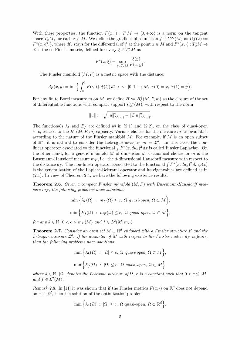
With these properties, the function F (x, ·) : TxM → [0,+∞) is a norm on the tangentspace TxM , for each x ∈M . We define the gradient of a function f ∈ C∞(M) as Df(x) :=F ∗(x, dfx), where dfx stays for the differential of f at the point x ∈M and F ∗(x, ·) : T ∗xM →R is the co-Finsler metric, defined for every ξ ∈ T ∗xM as

F ∗(x, ξ) = supy∈TxM

ξ(y)

F (x, y).

The Finsler manifold (M,F ) is a metric space with the distance:

dF (x, y) = inf∫ 1

0F (γ(t), γ(t)) dt : γ : [0, 1]→M, γ(0) = x, γ(1) = y

.

For any finite Borel measure m on M , we define H := H10 (M,F,m) as the closure of the set

of differentiable functions with compact support C∞c (M), with respect to the norm

‖u‖ :=√‖u‖2

L2(m)+ ‖Du‖2

L2(m).

The functionals λk and Ef are defined as in (2.1) and (2.2), on the class of quasi-opensets, related to the H1(M,F,m) capacity. Various choices for the measure m are available,according to the nature of the Finsler manifold M . For example, if M is an open subsetof Rd, it is natural to consider the Lebesgue measure m = Ld. In this case, the non-linear operator associated to the functional

∫F ∗(x, dux)2 dx is called Finsler Laplacian. On

the other hand, for a generic manifold M of dimension d, a canonical choice for m is theBusemann-Hausdorff measure mF , i.e. the d-dimensional Hausdorff measure with respect tothe distance dF . The non-linear operator associated to the functional

∫F ∗(x, dux)2 dmF (x)

is the generalization of the Laplace-Beltrami operator and its eigenvalues are defined as in(2.1). In view of Theorem 2.4, we have the following existence results:

Theorem 2.6. Given a compact Finsler manifold (M,F ) with Busemann-Hausdorff mea-sure mF , the following problems have solutions:

minλk(Ω) : mF (Ω) ≤ c, Ω quasi-open, Ω ⊂M

,

minEf (Ω) : mF (Ω) ≤ c, Ω quasi-open, Ω ⊂M

,

for any k ∈ N, 0 < c ≤ mF (M) and f ∈ L2(M,mF ).

Theorem 2.7. Consider an open set M ⊂ Rd endowed with a Finsler structure F and theLebesgue measure Ld. If the diameter of M with respect to the Finsler metric dF is finite,then the following problems have solutions:

minλk(Ω) : |Ω| ≤ c, Ω quasi-open, Ω ⊂M

,

minEf (Ω) : |Ω| ≤ c, Ω quasi-open, Ω ⊂M

,

where k ∈ N, |Ω| denotes the Lebesgue measure of Ω, c is a constant such that 0 < c ≤ |M |and f ∈ L2(M).

Remark 2.8. In [11] it was shown that if the Finsler metrics F (x, ·) on Rd does not dependon x ∈ Rd, then the solution of the optimization problem

minλ1(Ω) : |Ω| ≤ c, Ω quasi-open, Ω ⊂ Rd

,

5

is the ball of measure c. It is clear that it is also the case when in the hypotheses of Theorem2.7 one considers c > 0 such that there is a ball of measure c contained in M . On the otherhand , if c is big enough the solution is not, in general, the geodesic ball in M (see [15]).If the Finsler metric is not constant in x, the solution will not be a ball even for small c.In this case it is natural to ask whether the optimal set gets close to the geodesic ball asc → 0. In [18] this problem was discussed in the case when M is a Riemannian manifold.The same question for a generic Finsler manifold is still open.

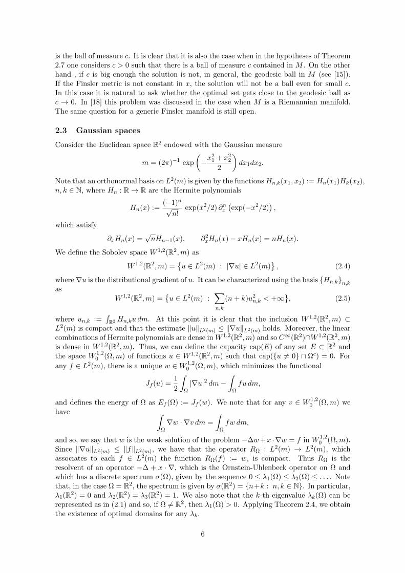
2.3 Gaussian spaces

Consider the Euclidean space R2 endowed with the Gaussian measure

m = (2π)−1 exp

(−x

21 + x2

2

2

)dx1dx2.

Note that an orthonormal basis on L2(m) is given by the functionsHn,k(x1, x2) := Hn(x1)Hk(x2),n, k ∈ N, where Hn : R→ R are the Hermite polynomials

Hn(x) :=(−1)n√n!

exp(x2/2) ∂nx(exp(−x2/2)

),

which satisfy

∂xHn(x) =√nHn−1(x), ∂2

xHn(x)− xHn(x) = nHn(x).

We define the Sobolev space W 1,2(R2,m) as

W 1,2(R2,m) =u ∈ L2(m) : |∇u| ∈ L2(m)

, (2.4)

where∇u is the distributional gradient of u. It can be characterized using the basis Hn,kn,kas

W 1,2(R2,m) =u ∈ L2(m) :

∑n,k

(n+ k)u2n,k < +∞

, (2.5)

where un,k :=∫R2 Hn,ku dm. At this point it is clear that the inclusion W 1,2(R2,m) ⊂

L2(m) is compact and that the estimate ‖u‖L2(m) ≤ ‖∇u‖L2(m) holds. Moreover, the linearcombinations of Hermite polynomials are dense in W 1,2(R2,m) and so C∞(R2)∩W 1,2(R2,m)is dense in W 1,2(R2,m). Thus, we can define the capacity cap(E) of any set E ⊂ R2 andthe space W 1,2

0 (Ω,m) of functions u ∈ W 1,2(R2,m) such that cap(u 6= 0 ∩ Ωc) = 0. For

any f ∈ L2(m), there is a unique w ∈W 1,20 (Ω,m), which minimizes the functional

Jf (u) =1

2

∫Ω|∇u|2 dm−

∫Ωfu dm,

and defines the energy of Ω as Ef (Ω) := Jf (w). We note that for any v ∈ W 1,20 (Ω,m) we

have ∫Ω∇w · ∇v dm =

∫Ωfw dm,

and so, we say that w is the weak solution of the problem −∆w+x ·∇w = f in W 1,20 (Ω,m).

Since ‖∇u‖L2(m) ≤ ‖f‖L2(m), we have that the operator RΩ : L2(m) → L2(m), whichassociates to each f ∈ L2(m) the function RΩ(f) := w, is compact. Thus RΩ is theresolvent of an operator −∆ + x · ∇, which is the Ornstein-Uhlenbeck operator on Ω andwhich has a discrete spectrum σ(Ω), given by the sequence 0 ≤ λ1(Ω) ≤ λ2(Ω) ≤ . . . . Notethat, in the case Ω = R2, the spectrum is given by σ(R2) = n+k : n, k ∈ N. In particular,λ1(R2) = 0 and λ2(R2) = λ3(R2) = 1. We also note that the k-th eigenvalue λk(Ω) can berepresented as in (2.1) and so, if Ω 6= R2, then λ1(Ω) > 0. Applying Theorem 2.4, we obtainthe existence of optimal domains for any λk.

6

Theorem 2.9. Consider R2 endowed with a non-degenerate Gaussian measure m, i.e. withinvertible covariance matrix. Then, for any k ∈ N, f ∈ L2(m) and 0 ≤ c ≤ 1, the followingoptimization problems have solutions:

minλk(Ω) : Ω ⊂ R2, m(Ω) ≤ c

,

minEf (Ω) : Ω ⊂ R2, m(Ω) ≤ c

,

which are quasi-open sets.

Remark 2.10. Theorem 2.9 also applies to penalized problems, i.e. for any Λ > 0, k ∈ Nand f ∈ L2(m), there is a solution of the problems

minλk(Ω) + Λm(Ω) : Ω ⊂ R2

, (2.6)

minEf (Ω) + Λm(Ω) : Ω ⊂ R2

, (2.7)

which is a quasi-open set. As we will see in the example below, these problems are sometimeseasier to threat when comes to regularity questions and qualitative study of the optimal sets.

Example 2.11. Let f be the constant 1 in Rd. By Remark 2.10, the problem (2.7) has asolution Ω, which we assume to be open and with boundary ∂Ω of class C2 (that we expectto be true), we can perform the shape derivative of the energy E1 with respect to somevector field V regular enough. Indeed, following [16, Chapter 5], let V : Rd → Rd be a C∞cvector field and for each t > 0 small enough, define Φt(x) = x + tV (x) and Ωt = Φt(Ω).Then, we have

dE1(Ωt)

dt

∣∣∣t=0

= −1

2

∫Ωw′ dm, (2.8)

where w′ is the solution of −∆w′ + x · ∇w′ = 0, in Ω,

w′ = −V · ∇w, on ∂Ω.(2.9)

We denote with w the (strong) solution of

−∆w + x · ∇w = 1, w ∈W 1,20 (Ω,m),

and integrate by parts in (2.8) obtaining

dE1(Ωt)

dt

∣∣∣t=0

= −1

2

∫Ω

(−∆w + x · ∇w)w′ dm = − 1

4π

∫∂Ω

∣∣∣∣∂w∂n∣∣∣∣2 V · n e−|x|2/2 dHd−1, (2.10)

where n is the exterior normal on ∂Ω and w is the energy function on Ω, that is the solutionof the Ornstein-Uhlenbeck PDE

−∆w + x · ∇w = 1 in Ω, w ∈W 1,20 (Ω,m).

On the other hand, we have

dm(Ωt)

dt

∣∣∣t=0

=1

2π

∫∂Ωe−|x|

2/2 V · ndHd−1, (2.11)

and so, by the optimality of Ω,(dE1(Ωt)

dt+ Λ

dm(Ωt)

dt

) ∣∣∣t=0

= 0

7

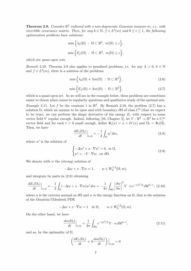
for any vector field V . By (2.10) and (2.11) we obtain∣∣∣∣∂w∂n∣∣∣∣ =√

2Λ on ∂Ω.

Summarizing, we have obtained that if an optimal domain Ω is regular enough, then thefollowing overdetermined boundary value problem has a solution:

−∆w + x · ∇w = 1, in Ω,

w = 0, on ∂Ω,∂w∂n = −

√2Λ, on ∂Ω.

(2.12)

It is straightforward to check that the following domains satisfy this condition:

• the half-space Ω = x1 > c, for a given c ∈ R,

• the strip Ω = |x1| < a, for some a > 0,

• the euclidean ball Ω = |x| < r, for some r > 0,

• the external domain of a ball Ω = |x| > r, for r > 0.

We do not know which of these domains is optimal and if there are other domains Ω forwhich the overdetermined problem (2.12) has a solution.

2.4 Carnot-Caratheodory spaces

Consider a bounded open and connected set D ⊂ Rd and C∞ vector fields Y1, . . . , Yn definedon a neighbourhood U of D. We say that the vector fields satisfy the Hormander’s conditionon U , if the Lie algebra generated by Y1, . . . , Yn has dimension d in each point x ∈ U .

We define the Sobolev space W 1,20 (D;Y ) on D with respect to the family of vector fields

Y = (Y1, . . . , Yn) as the closure of C∞c (D) with respect to the norm

‖u‖Y =

‖u‖2L2 +n∑

j=1

‖Yju‖2L2

1/2

,

where the derivation Yju is intended in sense of distributions. For u ∈W 1,20 (D;Y ), we define

the gradient Y u = (Y1u, . . . , Ynu) and set |Y u| =(|Y1u|2 + · · ·+ |Ynu|2

)1/2 ∈ L2(D).

Setting Du := |Y u| and H := W 1,20 (D;Y ), we define, for any Ω ⊂ D, the energy Ef (Ω)

and the kth eigenvalue λk(Ω) of the operator Y 21 + · · · + Y 2

n , as in (2.2) and (2.1). Thefollowing existence result is a consequence of Theorem 2.4.

Theorem 2.12. Consider a bounded open set D ⊂ Rd and a family Y = (Y1, . . . , Yn) ofC∞ vector fields defined on an open neighbourhood U of the closure D of D. If Y1, . . . , Ynsatisfy the Hormander condition on U , then for any k ∈ N, 0 < c ≤ |D| and f ∈ L2(D), thefollowing shape optimization problems admit a solution:

minλk(Ω) : Ω ⊂ D, Ω quasi-open, |Ω| ≤ c

, (2.13)

minEf (Ω) : Ω ⊂ D, Ω quasi-open, |Ω| ≤ c

. (2.14)

8

Proof. It is straightforward to check that the space H := W 1,20 (D;Y ) and the application

Du := |Y u| satisfy the assumptions of Theorem 2.4. The only non-trivial claim is the com-pact inclusion H ⊂ L2(D), which follows since Y1, . . . , Yn satisfy the Hormander conditionon U . In fact, by the Hormander Theorem (see [17]), there is some ε > 0 and some constantC > 0 such that for any ϕ ∈ C∞c (D)

‖ϕ‖Hε ≤ C

‖ϕ‖L2 +k∑

j=1

‖Yjϕ‖L2

, (2.15)

where we set

‖ϕ‖Hε =

(∫Rd

|ϕ(ξ)|2(1 + |ξ|2)ε dξ

)1/2

,

being ϕ the Fourier transform of ϕ. Let Hε0(D) be the closure of C∞c (D) with respect to the

norm ‖ · ‖Hε . Since the inclusion L2(D) ⊂ Hε0(D) is compact, we have the conclusion.

Remark 2.13. In the hypotheses of Theorem 2.12, the following optimization problems havea solution:

minλk(Ω) + Λ|Ω| : Ω ⊂ D, Ω quasi-open

, (2.16)

minEf (Ω) + Λ|Ω| : Ω ⊂ D, Ω quasi-open

, (2.17)

where k ∈ N, Λ > 0 and f ∈ L2(D) are given.

Example 2.14. Consider a bounded open set D ⊂ R2 and the vector fields X = ∂∂x and

Y = x ∂∂y . Since [X,Y ] = ∂

∂y , we can apply Theorem 2.12 and so, the shape optimizationproblem (2.17) has a solution Ω ⊂ D. Assuming that Ω is regular enough we may repeatthe argument from Section 2.3. Indeed, suppose that V is a vector field on ∂Ω and notethat the map Φt = Id + tV is a differomorphism for t small enough. Defining Ωt = Φt(Ω)and w the (strong) solution of

−(∂2x + x2∂2

y

)w + w = f, w ∈W 1,2

0 (Ω;X,Y ), (2.18)

where f ∈ L2(D), we have that

dEf (Ωt)

dt

∣∣∣t=0

= −1

2

∫Ωfw′ dx, (2.19)

where w′ is the weak solution of

−(∂2x + x2∂2

y

)w′ + w′ = 0, w′ + V · ∇w ∈W 1,2

0 (Ωt;X,Y ).

Using (2.18) and integrating by parts in (2.19), we obtain

dEf (Ωt)

dt

∣∣∣t=0

= −1

2

∫∂Ω

(V · ∇w)(n · (∂xw, x2∂yw)

)dH1. (2.20)

Sinced|Ωt|dt

∣∣∣t=0

=

∫∂ΩV · ndH1, (2.21)

we have that the energy function w is a solution of the following overdetermined boundaryvalue problem on the optimal set Ω

−(∂2x + x2∂2

y

)w + w = f in Ω,

w = 0 on ∂Ω,(n · (∂xw, x2∂yw)

)∂w∂n = 2Λ on ∂Ω.

(2.22)

The characterization of the solutions of (2.22) is an open problem even in the case f = 1.

9

3 Spectral optimization for metric graphs

In this section we study the problem of the optimization of the torsion rigidity of a onedimensional structure in Rd connecting a prescribed set of fixed points. Before we introducethe optimization problem we will examine some of the basic tools from the analysis of onedimensional sets.

Consider a closed connected set C ⊂ Rd of finite length H1(C) < ∞, where by H1 wedenote the one-dimensional Hausdorff measure in Rd. The natural choice of a distance onC is

dC(x, y) = inf

∫ 1

0|γ(t)| dt : γ : [0, 1]→ Rd Lipschitz, γ([0, 1]) ⊂ C, γ(0) = x, γ(1) = y

,

which, in turn, gives a pointwise definition of a gradient

|u′|(x) = lim supy→x

|u(y)− u(x)|d(x, y)

,

which is a function in L2(H1), at least in the case when u : C → R is Lipschitz with respectto the distance dC . For any function u : C → R, Lipschitz with respect to the distance dC ,we define the norm

‖u‖2H1(C) =

∫Cu2 dH1 +

∫C|u′|2 dH1,

and the Sobolev space H1(C), as the closure of the Lipschitz functions on C with respect tothis norm. By the Second Rectifiability Theorem (see [2, Theorem 4.4.8]) the set C consistsof a countable family of injective arc-length parametrized Lipschitz curves γi : [0, li] → C,i ∈ N, i.e. there is an H1-negligible set N ⊂ C such that C = N ∪ (∪i γi([0, li])). On each

curve γi we have the chain rule∣∣∣ ddtu(γi(t))

∣∣∣ = |u′|(γi(t)) (see [8, Lemma 3.1] for a proof)

and thus, we obtain the following expression for the norm of u ∈ H1(C):

‖u‖2H1(C) =

∫Cu2 dH1 +

∑i

∫ li

0

∣∣∣∣ ddtu(γi(t))

∣∣∣∣2 dt. (3.1)

Given a set of distinct pointsD1, . . . , Dk ∈ Rd we define the admissible classAC(D1, . . . , Dk)as the family of closed connected sets C ⊂ Rd containing D1, . . . , Dk. For any C ∈AC(D1, . . . , Dk) we consider the space of Sobolev functions which satisfy a Dirichlet condi-tion at the points Di:

H10 (C;D1, . . . , Dk) = u ∈ H1(C) : u(Dj) = 0, j = 1 . . . , k.

For the points Dj we use the term Dirichlet points. The Dirichlet Energy of the set C withrespect to D1, . . . , Dk is defined as

E(C;D1, . . . , Dk) = minu∈H1

0 (C;D1,...,Dk)

1

2

∫C|u′|2 dH1 −

∫Cu dH1. (3.2)

We study the following shape optimization problem:

minE(C;D1, . . . , Dk) : C ∈ AC(D1, . . . , Dk), H1(C) ≤ l

. (3.3)

Remark 3.1. We note that the admissible sets C can be reduced to the set of graphsembedded in Rd. For sake of simplicity, we limit ourselves to the case of three pointsD1, D2, D3 ∈ Rd (for the general result see [8]). Let C ∈ AC(D1, D2, D3) be such that

10

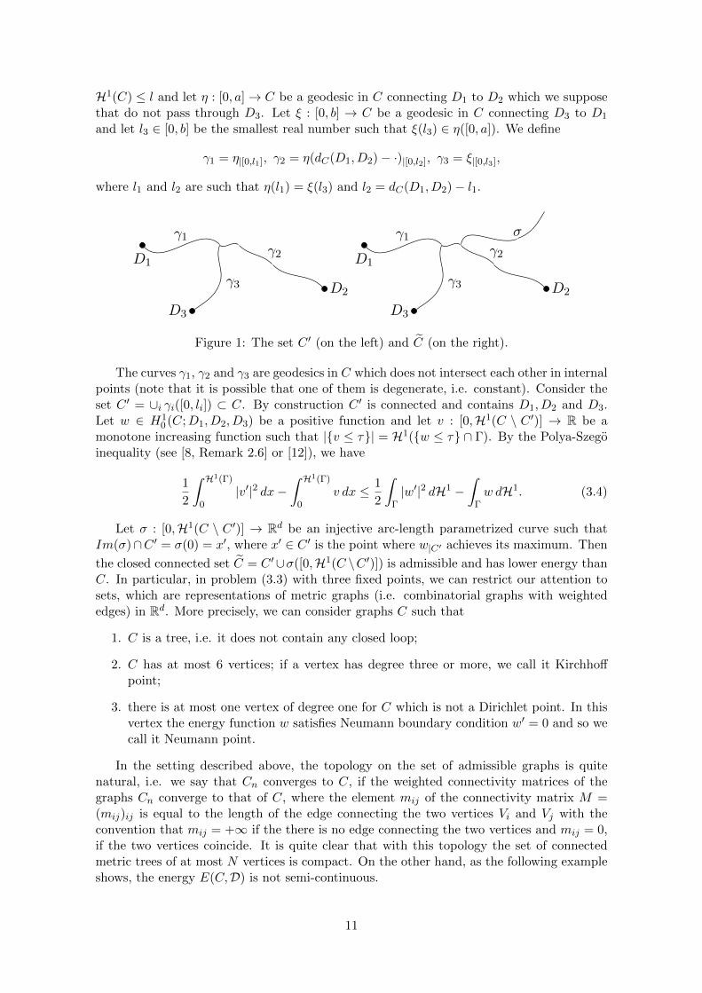
H1(C) ≤ l and let η : [0, a]→ C be a geodesic in C connecting D1 to D2 which we supposethat do not pass through D3. Let ξ : [0, b] → C be a geodesic in C connecting D3 to D1

and let l3 ∈ [0, b] be the smallest real number such that ξ(l3) ∈ η([0, a]). We define

γ1 = η|[0,l1], γ2 = η(dC(D1, D2)− ·)|[0,l2], γ3 = ξ|[0,l3],

where l1 and l2 are such that η(l1) = ξ(l3) and l2 = dC(D1, D2)− l1.

D1

γ1γ2

D2γ3

D3

D1

γ1γ2

D2

σ

γ3

D3

1

D1

γ1γ2

D2γ3

D3

D1

γ1γ2

D2

σ

γ3

D3

1

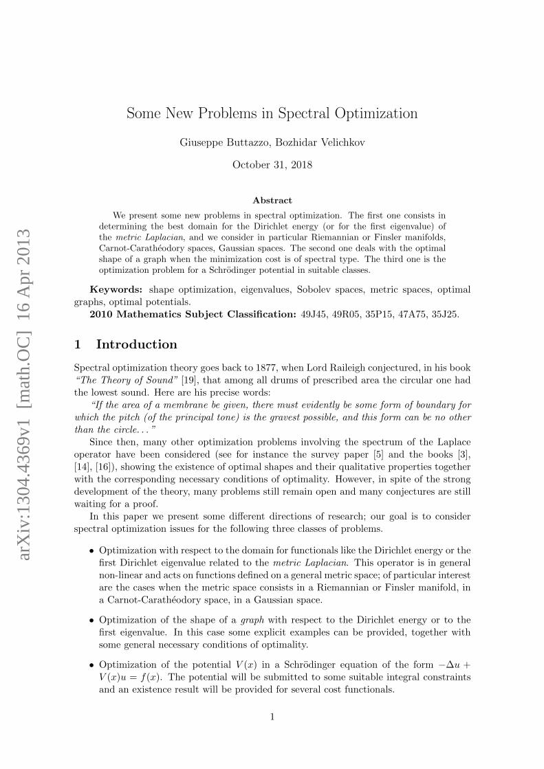
Figure 1: The set C ′ (on the left) and C (on the right).

The curves γ1, γ2 and γ3 are geodesics in C which does not intersect each other in internalpoints (note that it is possible that one of them is degenerate, i.e. constant). Consider theset C ′ = ∪i γi([0, li]) ⊂ C. By construction C ′ is connected and contains D1, D2 and D3.Let w ∈ H1

0 (C;D1, D2, D3) be a positive function and let v : [0,H1(C \ C ′)] → R be amonotone increasing function such that |v ≤ τ| = H1(w ≤ τ ∩ Γ). By the Polya-Szegoinequality (see [8, Remark 2.6] or [12]), we have

1

2

∫ H1(Γ)

0|v′|2 dx−

∫ H1(Γ)

0v dx ≤ 1

2

∫Γ|w′|2 dH1 −

∫Γw dH1. (3.4)

Let σ : [0,H1(C \ C ′)] → Rd be an injective arc-length parametrized curve such thatIm(σ)∩C ′ = σ(0) = x′, where x′ ∈ C ′ is the point where w|C′ achieves its maximum. Then

the closed connected set C = C ′∪σ([0,H1(C \C ′)]) is admissible and has lower energy thanC. In particular, in problem (3.3) with three fixed points, we can restrict our attention tosets, which are representations of metric graphs (i.e. combinatorial graphs with weightededges) in Rd. More precisely, we can consider graphs C such that

1. C is a tree, i.e. it does not contain any closed loop;

2. C has at most 6 vertices; if a vertex has degree three or more, we call it Kirchhoffpoint;

3. there is at most one vertex of degree one for C which is not a Dirichlet point. In thisvertex the energy function w satisfies Neumann boundary condition w′ = 0 and so wecall it Neumann point.

In the setting described above, the topology on the set of admissible graphs is quitenatural, i.e. we say that Cn converges to C, if the weighted connectivity matrices of thegraphs Cn converge to that of C, where the element mij of the connectivity matrix M =(mij)ij is equal to the length of the edge connecting the two vertices Vi and Vj with theconvention that mij = +∞ if the there is no edge connecting the two vertices and mij = 0,if the two vertices coincide. It is quite clear that with this topology the set of connectedmetric trees of at most N vertices is compact. On the other hand, as the following exampleshows, the energy E(C,D) is not semi-continuous.

11

Example 3.2. Consider the points D1 = (0, 0), D2 = (1, 0) and D3 = (2, 0) and the setCn ⊂ R2 consisting of the graphs of the functions y(x) = x(x − 1) for x ∈ [0, 1] andyn(x) = − 1

nx(x − 2) for x ∈ [0, 2]. Passing to the limit as n → ∞, we have that the arcconnecting D1 to D3 passes through the Dirichlet point D2 which causes the energy tosuddenly increase.

Remark 3.3. The lack of semi-continuity does not necessarily imply the non-existence ofa solution of (3.3), but suggests the nature of a possible counter-example. Following thisidea, in [8], was proved that if D = D1, D2, D3 ⊂ R2 is a set of points, with coordinatesrespectively (−1, 0), (1, 0) and (n, 0), and l = n + 2 is a given length, then, for n largeenough, the problem (3.3) does not have a solution.

In order to obtain an existence result for the problem (3.3), we consider, as in [8],in a larger class of admissible sets. Indeed, let Γ be a combinatorial graph with verticesVii=1,...,N and edges eijij . We call Γ a metric graph, if to each edge eij is associated apositive real number lij which we interpret as the length of the edge. Thus, the total lengthof Γ is given by l(Γ) :=

∑i<j lij .

A function u : Γ→ Rn on the metric graph Γ is a collection of functions uij : [0, lij ]→ R,for 1 ≤ i 6= j ≤ N , such that:

1. uji(x) = uij(lij − x), for each 1 ≤ i 6= j ≤ N ,

2. uij(0) = uik(0), for all i, j, k ⊂ 1, . . . , N.

We say that u is continuous (u ∈ C(Γ)), square integrable u ∈ L2(Γ) or Sobolev u ∈ H1(Γ),if uij is respectively continuous, square integrable or Sobolev on each edge eij . We also notethat, if u ∈ H1(Γ), then |u′| ∈ L2(Γ) and so, we can define

E(Γ; V1, . . . , Vk) = minu∈H1

0 (Γ;V1,...,Vk)

1

2

∫Γ|u′|2 dH1 −

∫Γu dH1, (3.5)

where H10 (Γ; V1, . . . , Vk) indicates the subspace of H1(Γ) of the functions vanishing on

each of the vertices V1, . . . , Vk and we also used the notation∫Γ|u′|2 dH1 :=

∑ij

∫ lij

0|u′ij |2 dx,

∫Γu dH1 :=

∑ij

∫ lij

0uij dx.

We say that the continuous function γ = (γij)1≤i 6=j≤N : Γ→ Rd is an immersion of themetric graph Γ into Rd, if for each 1 ≤ i 6= j ≤ N the function γij : [0, lij ] → Rd is aninjective arc-length parametrized curve. Given a set of distinct points D1, . . . , Dk ∈ Rd, wedefine the admissible set A(D1, . . . , Dk) as the set of metric graphs Γ for which there is animmersion γ : Γ → Rd such that γ(Vi) = Di, where V1, . . . , Vk are vertices of Γ. In [8] thefollowing result was proved.

Theorem 3.4. Consider a set of distinct points D1, . . . , Dk ∈ Rd and a real number l suchthat there is a closed set C ⊂ Rd which contains D1, . . . , Dk and such that H1(C) ≤ l. Thenthe following problem has a solution:

minE(Γ; V1, . . . , Vk) : Γ ∈ A(D1, . . . , Dk), l(Γ) ≤ l

. (3.6)

In some situations, we can use Theorem 3.4 to obtain an existence result for (3.3).

Proposition 3.5. Suppose that D1, D2 and D3 be three distinct, non co-linear points inRd and let l > 0 be a real number such that there exists a closed set of length l connectingD1, D2 and D3. Then the problem (3.3) has a solution.

12

Proof. Let the graph Γ be a solution of (3.6) and let γ : Γ→ Rd be an immersion of Γ suchthat γ(Vj) = Dj for j = 1, 2, 3. Note that if the immersion γ is such that the set γ(Γ) ⊂ Rd

is represented by the same graph Γ, then γ(Γ) is a solution of (3.3) since we have

E(Γ; V1, V2, V3) = E(C;D1, D2, D3).

Reasoning as in Remark 3.1, we can suppose that Γ is obtained by a tree Γ′ with verticesV1, V2 and V3 by attaching a new edge (with a new vertex in one of the extrema) to somevertex or edge of Γ′. Since we are free to choose the immersion of the new edge, we onlyneed to show that we can choose γ in order to have that the set γ(Γ′) is represented by Γ′.On the other hand we have only two possibilities for Γ′ and both of them can be seen asembedded graphs in Rd with vertices D1, D2 and D3.

Remark 3.6. Similarly to the existence proof of a classical optimal graph of Propositionabove we believe that a more general result should hold: if D1, . . . , Dk are k distinct pointsin Rd such that none of them can be expressed as a convex combination of the others, then(3.3) has a solution. We do not yet have a complete proof of this fact.

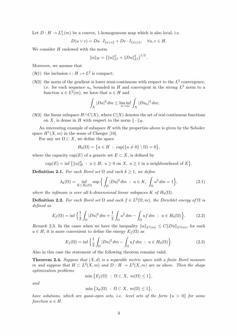
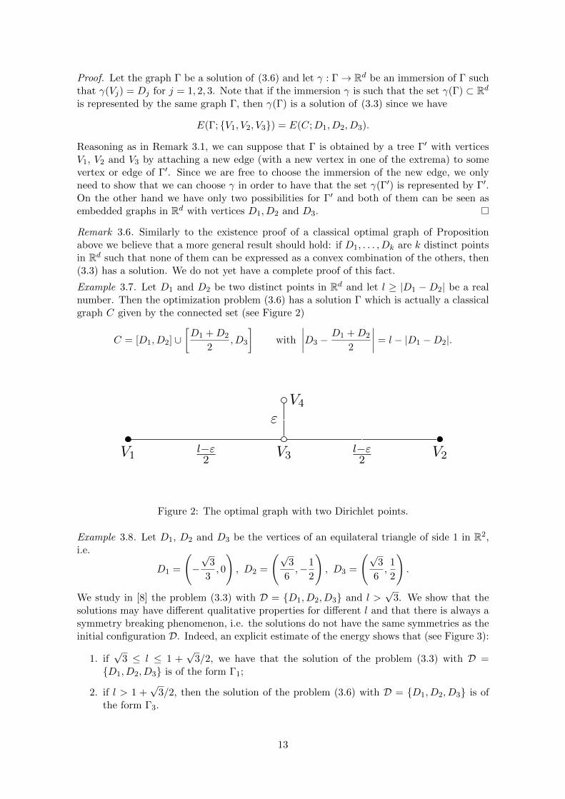
Example 3.7. Let D1 and D2 be two distinct points in Rd and let l ≥ |D1 −D2| be a realnumber. Then the optimization problem (3.6) has a solution Γ which is actually a classicalgraph C given by the connected set (see Figure 2)

C = [D1, D2] ∪[D1 +D2

2, D3

]with

∣∣∣∣D3 −D1 +D2

2

∣∣∣∣ = l − |D1 −D2|.

V1l−ε2

V3l−ε2

V2

εV4

1

Figure 2: The optimal graph with two Dirichlet points.

Example 3.8. Let D1, D2 and D3 be the vertices of an equilateral triangle of side 1 in R2,i.e.

D1 =

(−√

3

3, 0

), D2 =

(√3

6,−1

2

), D3 =

(√3

6,1

2

).

We study in [8] the problem (3.3) with D = D1, D2, D3 and l >√

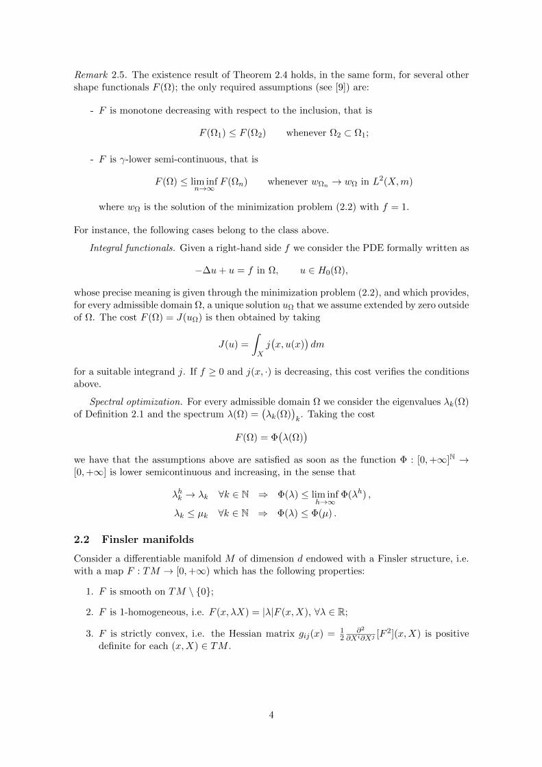
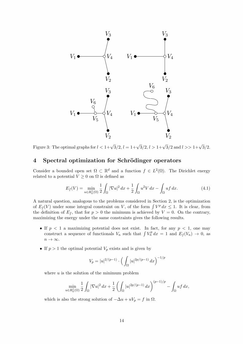
3. We show that thesolutions may have different qualitative properties for different l and that there is always asymmetry breaking phenomenon, i.e. the solutions do not have the same symmetries as theinitial configuration D. Indeed, an explicit estimate of the energy shows that (see Figure 3):

1. if√

3 ≤ l ≤ 1 +√

3/2, we have that the solution of the problem (3.3) with D =D1, D2, D3 is of the form Γ1;

2. if l > 1 +√

3/2, then the solution of the problem (3.6) with D = D1, D2, D3 is ofthe form Γ3.

13

V1

V2

V3

V4 V1

V2

V3

V4 V1

V2

V3

V5

V4

V6

V1

V2

V3

V5

V4

V6

(a)l <√3/2 + 1 (b) l =

√3/2 + 1 (c) l >

√3/2 + 1 (d) l >>

√3/2 + 1

V1

V2

V3

V4 V1

V2

V3

V4 V1

V2

V3

V5

V4

V6

V1

V2

V3

V5

V4

V6

(a)l <√3/2 + 1 (b) l =

√3/2 + 1 (c) l >

√3/2 + 1 (d) l >>

√3/2 + 1Figure 3: The optimal graphs for l < 1+

√3/2, l = 1+

√3/2, l > 1+

√3/2 and l >> 1+

√3/2.

4 Spectral optimization for Schrodinger operators

Consider a bounded open set Ω ⊂ Rd and a function f ∈ L2(Ω). The Dirichlet energyrelated to a potential V ≥ 0 on Ω is defined as

Ef (V ) = minu∈H1

0 (Ω)

1

2

∫Ω|∇u|2 dx+

1

2

∫Ωu2V dx−

∫Ωuf dx. (4.1)

A natural question, analogous to the problems considered in Section 2, is the optimizationof Ef (V ) under some integral constraint on V , of the form

∫V p dx ≤ 1. It is clear, from

the definition of Ef , that for p > 0 the minimum is achieved by V = 0. On the contrary,maximizing the energy under the same constraints gives the following results.

• If p < 1 a maximizing potential does not exist. In fact, for any p < 1, one mayconstruct a sequence of functionals Vn such that

∫V pn dx = 1 and Ef (Vn) → 0, as

n→∞.

• If p > 1 the optimal potential Vp exists and is given by

Vp = |u|2/(p−1) ·(∫

Ω|u|2p/(p−1) dx

)−1/p

where u is the solution of the minimum problem

minu∈H1

0 (Ω)

1

2

∫Ω|∇u|2 dx+

1

2

(∫Ω|u|2p/(p−1) dx

)(p−1)/p

−∫

Ωuf dx,

which is also the strong solution of −∆u+ uVp = f in Ω.

14

• If p = 1 the optimal potential V1 exists and is given by

V1 =f

M

(1ω+ − 1ω−

),

where M = ‖u1‖L∞(Ω), ω+ = u1 = M, ω− = u1 = −M, and u1 ∈ H10 (Ω)∩H2(Ω)

is the unique minimizer of the functional J1 : L2(Ω)→ R, defined as

J1(u) :=1

2

∫Ω|∇u|2 dx+

1

2‖u‖2L∞(Ω) −

∫Ωuf dx.

In particular, we have∫ω+

f dx−∫ω−

f dx = M, f ≥ 0 on ω+, f ≤ 0 on ω− .

Example 4.1. Let Ω = (−1, 1) and f be a positive constant on Ω. Then u1 is positiveand, by a symmetrization argument, it is also radially symmetric and decreasing. Thus,ω+ = (−a, a) for some a ∈ (0, 1) and since |ω+|M = 1, we have that a = 1

2M . Sinceu′( 1

2M ) = 0 and u′′ = −f on ( 12M , 1), we have that (1 − 1

2M )2f = 2M , which uniquelydetermines M and so, the optimal potential V1 = 1

M 1(− 12M

, 12M

).

When p < 0 the minimization problem

min

Ef (V ) : V : Ω→ [0,+∞],

∫ΩV p dx = 1

, (4.2)

becomes meaningful.

Proposition 4.2. Let Ω ⊂ Rd be a bounded open set and let f ∈ L2(Ω). Then, for everyp < 0, the problem (4.2) has a solution.

Proof. By the definition of Ef (V ), interchanging the two min operators, we find that theoptimal potential Vp is given by

Vp = |u|2/(p−1) ·(∫

Ω|u|2p/(p−1) dx

)−1/p(4.3)

where u is the solution of the minimum problem

minu∈H1

0 (Ω)

1

2

∫Ω|∇u|2 dx+

1

2

(∫Ω|u|2p/(p−1) dx

)(p−1)/p

−∫

Ωuf dx. (4.4)

Note that, since p < 0, the quantity q = 2p/(p − 1) is such that 0 < q < 2. The existenceof a solution for problem (4.4) is straightforward, which gives the existence of the optimalpotential Vp through equality (4.3).

When we consider more general cost functionals F (V ), like for instance spectral costsdepending on the eigenvalues of the Schrodinger operator −∆ + V , the proof above cannotbe repeated; nevertheless, using finer tools like γ-convergence for Dirichlet problems, thefollowing more general result can be obtained (see [7]).

Theorem 4.3. Consider a cost functional F : B+(Ω)→ R, where B+(Ω) denotes the spaceof Borel measurable positive functions on Ω. Suppose that F is

1. increasing, i.e. F (V ) ≥ F (W ), whenever V ≥W ;

15

2. lower semi-continuous with respect to strong convergence of the resolvents

RV = (−∆ + V )−1 : L2(Ω)→ L2(Ω).

Then, for any p < 0, the optimization problem

min

F (V ) : V : Ω→ [0,+∞],

∫ΩV p dx = 1

,

has a solution.

Acknowledgements. The second author wish to thank Gian Maria Dall’Ara for theuseful discussions.

References

[1] L. Ambrosio, N. Fusco, D. Pallara: Function of Bounded Variation and FreeDiscontinuity Problems. Oxford University Press, Oxford (2000).

[2] L. Ambrosio, P. Tilli: Topics on Analysis in Metric Spaces. Oxford Lecture Seriesin Mathematics and its Applications, Oxford University Press, Oxford (2004).

[3] D. Bucur, G. Buttazzo: Variational Methods in Shape Optimization Problems.Progress in Nonlinear Differential Equations 65, Birkhauser Verlag, Basel (2005).

[4] D. Bucur, G. Buttazzo, B. Velichkov: Spectral optimization problems with in-ternal constraint. Ann. Inst. H. Poincare Anal. Non Lineaire, (to appear), preprintavailable at http://cvgmt.sns.it.

[5] G. Buttazzo: Spectral optimization problems. Rev. Mat. Complut., 24 (2) (2011),277–322.

[6] G. Buttazzo, G. Dal Maso: An existence result for a class of shape optimizationproblems. Arch. Rational Mech. Anal., 122 (1993), 183–195.

[7] G. Buttazzo, A. Gerolin, B. Ruffini, B. Velichkov: Optimal potentials forSchrodinger operators. Paper in preparation.

[8] G. Buttazzo, B. Ruffini, B. Velichkov: Shape optimization problems for metricgraphs. Preprint 2012, available at http://cvgmt.sns.it.

[9] G. Buttazzo, B. Velichkov: Shape optimization problems on metric measurespaces. J. Funct. Anal., (to appear), preprint available at http://cvgmt.sns.it.

[10] J. Cheeger: Differentiability of Lipschitz functions on metric measure spaces. Geom.Funct. Anal., 9 (3) (1999), 428–517.

[11] V. Ferone, B. Kawohl: Remarks on a Finsler-Laplacian. Proceedings of the AMS,137 (2007), no. 1, 247–253.

[12] L. Friedlander: Extremal properties of eigenvalues for a metric graph. Ann. Inst.Fourier, 55 (1) (2005), 199–211.

[13] A. Henrot: Minimization problems for eigenvalues of the Laplacian. J. Evol. Equ.,3 (3) (2003), 443–461.

16

[14] A. Henrot: Extremum Problems for Eigenvalues of Elliptic Operators. Frontiers inMathematics, Birkhauser Verlag, Basel (2006).

[15] A. Henrot, E. Oudet: Le stade ne minimise pas λ2 parmi les ouverts convexes duplan. C. R. Acad. Sci. Paris Sr. I Math, 332 (4) (2001), 275–280.

[16] A. Henrot, M. Pierre: Variation et Optimisation de Formes: une AnalyseGeometrique. Springer-Verlag, Berlin (2005).

[17] L. Hormander: Hypoelliptic second-order differential equations. Acta Math., 119(1967), 147–171.

[18] F. Pacard, P. Sicbaldi: Extremal domains for the first eigenvalue of the Laplace-Beltrami operator. Annalles de l’Institut Fourier 59, no.2 (2009), 515–542.

[19] L. Rayleigh: The Theory of Sound. 1st edition, Macmillan, London (1877).

Giuseppe ButtazzoDipartimento di MatematicaUniversita di PisaLargo B. Pontecorvo, 556127 Pisa - ITALYbuttazzo@dm.unipi.it

Bozhidar VelichkovScuola Normale Superiore di PisaPiazza dei Cavalieri, 756126 Pisa - ITALYb.velichkov@sns.it

17