python-deltasigma documentationRelease 0.2.0

Giuseppe Venturini

July 28, 2015

Contents

1 Contents 3

2 Status 5

3 Examples 7

4 Install 94.1 Supported platforms . . . . . . . . . . . . . . . . . . . . . . . . . . . . . . . . . . . . . . . . . 94.2 Required dependencies . . . . . . . . . . . . . . . . . . . . . . . . . . . . . . . . . . . . . . . . 94.3 Optional (but recommended) dependencies . . . . . . . . . . . . . . . . . . . . . . . . . . . . . 94.4 Install the deltasigma package . . . . . . . . . . . . . . . . . . . . . . . . . . . . . . . . . . . . 104.5 Extras for developers . . . . . . . . . . . . . . . . . . . . . . . . . . . . . . . . . . . . . . . . . 10

5 Useful resources 11

6 How to contribute 136.1 Pull requests are welcome! . . . . . . . . . . . . . . . . . . . . . . . . . . . . . . . . . . . . . . 136.2 Reporting bugs . . . . . . . . . . . . . . . . . . . . . . . . . . . . . . . . . . . . . . . . . . . . 136.3 Support python-deltasigma . . . . . . . . . . . . . . . . . . . . . . . . . . . . . . . . . . . . . . 13

7 License, copyright, rationale and credits 157.1 Why this project was born . . . . . . . . . . . . . . . . . . . . . . . . . . . . . . . . . . . . . . 157.2 Licensing and copyright notice . . . . . . . . . . . . . . . . . . . . . . . . . . . . . . . . . . . 157.3 Credits . . . . . . . . . . . . . . . . . . . . . . . . . . . . . . . . . . . . . . . . . . . . . . . . 15

8 Implementation model 178.1 Modulator model . . . . . . . . . . . . . . . . . . . . . . . . . . . . . . . . . . . . . . . . . . . 178.2 Topologies diagrams . . . . . . . . . . . . . . . . . . . . . . . . . . . . . . . . . . . . . . . . . 188.3 Discrete time to continuous time mapping . . . . . . . . . . . . . . . . . . . . . . . . . . . . . . 24

9 Package contents 279.1 Key Functions . . . . . . . . . . . . . . . . . . . . . . . . . . . . . . . . . . . . . . . . . . . . 279.2 Functions for quadrature delta-sigma modulators . . . . . . . . . . . . . . . . . . . . . . . . . . 279.3 Other selected functions . . . . . . . . . . . . . . . . . . . . . . . . . . . . . . . . . . . . . . . 279.4 Utility functions for simulation of delta-sigma modulators . . . . . . . . . . . . . . . . . . . . . 289.5 General utilities for data processing . . . . . . . . . . . . . . . . . . . . . . . . . . . . . . . . . 289.6 Plotting and data display utilitites . . . . . . . . . . . . . . . . . . . . . . . . . . . . . . . . . . 29

10 All functions in alphabetical order 31

Bibliography 73

Python Module Index 75

i

ii

A port of the MATLAB Delta Sigma Toolbox based on free software and very little sleep.

Author Giuseppe Venturini, based on Richard Schreier’s work, who deserves most of the credit.

Release 0.2.0

Date July 28, 2015

Homepage: http://www.python-deltasigma.io

Documentation: http://docs.python-deltasigma.io

Repository: https://github.com/ggventurini/python-deltasigma

Bug tracker: https://github.com/ggventurini/python-deltasigma/issues

Python-deltasigma is a Python package to synthesize, simulate, scale and map to implementable structures deltasigma modulators.

It aims to provide a 1:1 Python port of Richard Schreier’s *excellent* MATLAB Delta Sigma Toolbox, the defacto standard tool for high-level delta sigma simulation, upon which it is very heavily based.

1

2

CHAPTER 1

Contents

3

Contents

• Introduction• Contents• Status• Examples• Install

– Supported platforms– Required dependencies– Optional (but recommended) dependencies– Install the deltasigma package– Extras for developers

• Useful resources• How to contribute

– Pull requests are welcome!– Reporting bugs– Support python-deltasigma

• License, copyright, rationale and credits– Why this project was born– Licensing and copyright notice– Credits

• Implementation model– Modulator model

* The loop filter* Quantizer model

– Topologies diagrams* CIFB* CIFF* CRFB* CRFF* CRFBD* CRFFD

– Discrete time to continuous time mapping* 1: equate the loop filter transfer functions* 2: match the loop filter impulse responses* 3: match the DT NTF and CT filter pulse responses

• Package contents– Key Functions– Functions for quadrature delta-sigma modulators– Other selected functions– Utility functions for simulation of delta-sigma modulators– General utilities for data processing– Plotting and data display utilitites

• All functions in alphabetical order

4

CHAPTER 2

Status

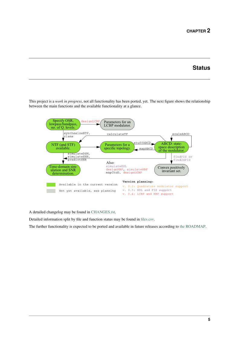
This project is a work in progress, not all functionality has been ported, yet. The next figure shows the relationshipbetween the main functions and the available functionality at a glance.

A detailed changelog may be found in CHANGES.rst.

Detailed information split by file and function status may be found in files.csv.

The further functionality is expected to be ported and available in future releases according to the ROADMAP.

5

6

CHAPTER 3

Examples

To see the currently implemented functionality in action, take a look at the following ipython notebooks:

• dsdemo1, notebook port of the interactive dsdemo1.m.

• dsdemo2, notebook port of the interactive dsdemo2.m.

• dsdemo3, notebook port of the interactive dsdemo3.m.

• dsdemo4, notebook port of dsdemo4.m. Audio file, right click to download.

• MASH example, an example of the simulation of a MASH cascade.

• dsexample1, Python version of dsexample1.m.

• dsexample2, Python version of dsexample2.m.

• dsexample3, Python version of dsexample3.m.

They are also a good means for getting started quickly.

If you have some examples you would like to share, send me a mail, and I will add them to the above list.

7

8

CHAPTER 4

Install

4.1 Supported platforms

python-deltasigma runs on every platform and arch. supported by its dependencies:

• Platforms: Linux, Mac OS X, Windows.

• Archs: x86, x86_64 and armf (arm with floating point unit).

4.2 Required dependencies

Using python-deltasigma requires Python 2 or 3, at your choice, numpy, scipy (>= 0.11.0) and matplotlib.

They are packaged by virtually all the major Linux distributions.

On a Debian Linux system, you may install them issuing:

aptitude install python python-numpy python-scipy python-matplotlib

Refer to your system documentation for more information.

On Windows, I hear good things about:

• Enthought Canopy, a Python distribution that carries both free and commercial versions, and

• Anaconda, which offers its full version for free.

I do not run Windows, so I can’t really provide more info (sorry), except that people tell me they manage to havea working setup.

Mac OS X is also supported by Enthought Canopy and Anaconda, which likely provide the easiest and fastestsolution to have a scientific Python stack up and running.

More information can be found on the scipy install page and on the matplotlib homepage.

I wrote in a different context some directions to compile numpy and scipy yourself, which also apply here. Bewarned, it can easily get complicated.

4.3 Optional (but recommended) dependencies

The required dependencies have been kept to a minimum to allow running python-deltasigma on worksta-tions that are not managed by the user but by a system administrator - where typically installing libraries is notpossible and software packages are disarmingly outdated.

If at all possible, installing Cython is strongly recommended.

9

python-deltasigma contains python extension to simulate delta sigma modulators providing a near-nativeexecution speed – overall roughly a 70x speed-up compared to a plain Python implementation.

On Linux, installing Cython is just one: aptitude install cython away.

On Mac OS X and Windows, Cython may be installed as part of one of the frameworks above. Please notice acompiler is needed, this may require installing XCode and its command-line utilities or gcc through homebrew,on Mac OS X, or Mingw, on Windows.

If the BLAS headers are found on the machine, they will be used. In case they cannot be found automatically, it isrecommended to set the environment variable BLAS_H to the BLAS headers directory.

On Mac OS X, consider linking the headers to their conventional location:

sudo ln -s /System/Library/Frameworks/Accelerate.framework/Versions/Current/Frameworks/vecLib.framework/Versions/Current/Headers/cblas.h /usr/include/cblas.h

The Cython extensions were written by Sergio Callegari, please see the deltasigma/ for copyright notice andmore information.

4.4 Install the deltasigma package

Once the dependencies set up, it is possible to install the latest stable version directly from the Python PackageIndex (PYPI), running:

pip install deltasigma

The above command will also attempt to compile and install the dependencies in case they are not found. Pleasenotice this is not recommended and for this to work you should already have the required C libraries in place.

If you are interested in a bleeding-edge version – potentially less stable – or in contributing code (that’s awesome!)you can head over to the Github repository and check out the code from there.

Then run:

python setup.py install

The flag --user may be an interesting option to install the package for the current user only, and it doesn’trequire root privileges.

4.5 Extras for developers

The following may be installed at a later stage and are typically only necessary for developers.

Building the documentation requires the sphinx package. It is an optional step, as the the latest documentation isavailable on line, without need for you to build it.

If you plan to modify the code, python-deltasigma comes with a complete unit tests suite, which is run againstevery commit and that any addition should pass both for Python 2 and 3. To run it locally, setuptools is needed, asit is used to access the reference function outputs.

Running the test suite may be conveniently automated installing nose, and then issuing:

nosetests -v deltasigma

from the repository root.

10

CHAPTER 5

Useful resources

The original MATLAB Toolbox provides in-depth documentation, which is very useful to understand what thetoolbox is capable of. See DSToolbox.pdf and OnePageStory.pdf (PDF warning).

The book:

Richard Schreier, Gabor C. Temes, Understanding Delta-Sigma Data Converters, ISBN: 978-0-471-46585-0, November 2004, Wiley-IEEE Press

is probably the most authoritative resource on the topic. Chapter 8-9 show how to use the MATLAB toolkit andthe observations apply also to this Python port. Links on amazon, on the Wiley-IEEE press.

I am not affiliated with neither the sellers nor the authors.

11

12

CHAPTER 6

How to contribute

6.1 Pull requests are welcome!

If you want to port some code, fix a bug, add a cool example or implement new functionality (in this case it maybe a good idea to get in touch early on), that’s awesome!

There are only a few guidelines, which can be overridden every time it is reasonable to do so:

• Please try to follow PEP8.

• Try to keep the functions signature identical. Parameters with NaN default values have their default valuereplaced with None.

• If a function has a variable number of return values, its Python port should implement the maximum numberof return values.

No commit should ever fail the test suite.

6.2 Reporting bugs

What bugs, there are no bugs!

Jokes aside, please report all bugs on on the Github issue tracker.

6.3 Support python-deltasigma

I do not want your money. I develop this software because I enjoy it and because I use it myself.

If you wish to support the development of python-deltasigma or you find the package useful or you other-wise wish to contribute monetarily, *please donate to cancer research instead:*

• Association for International Cancer Research (eng), or

• Fond. IRCCS Istituto Nazionale dei Tumori (it).

Consider sending me a mail afterwards, *it makes for great motivation!*

13

14

CHAPTER 7

License, copyright, rationale and credits

7.1 Why this project was born

I like challenges, delta-sigma modulation and I don’t have the money for my own MATLAB license. After all,which grad student or young researcher has it?

With this Python package you can simulate delta-sigma modulators for free, on any PC.

I hope you find it useful.

7.2 Licensing and copyright notice

All original MATLAB code is Copyright (c) 2009, Richard Schreier. See the LICENSE file for the licensing terms.

The Python code here provided is a derivative work from the above toolkit and subject to the same license terms.

Credit goes to Richard Schreier for the original ideas, their MATLAB implementation and the all the diagramsfound in this documentation. Little-to-no conceptual improvements are introduced here, just code adaptation,refactoring, rewrites and fixing of a few minor issues.

This package contains some source code from pydsm, also based on the same MATLAB toolbox. The pydsmpackage is copyright (c) 2012, Sergio Callegari.

When not otherwise specified, the Python code is Copyright 2013, Giuseppe Venturini and the python-deltasigmacontributors.

MATLAB is a registered trademark of The MathWorks, Inc.

7.3 Credits

The python-deltasigma package was written by Giuseppe Venturini, as a derivative work of RichardSchreier’s MATLAB Delta Sigma toolbox. It contains code from pydsm, also based on the same MATLABtoolbox and written by Sergio Callegari.

Contributors: Shayne Hodge

15

16

CHAPTER 8

Implementation model

The internal implementation of delta sigma modulators follows closely the one in Richard Schreier’s MATLABDelta Sigma Toolbox, upon which the following documentation is very heavily based.

8.1 Modulator model

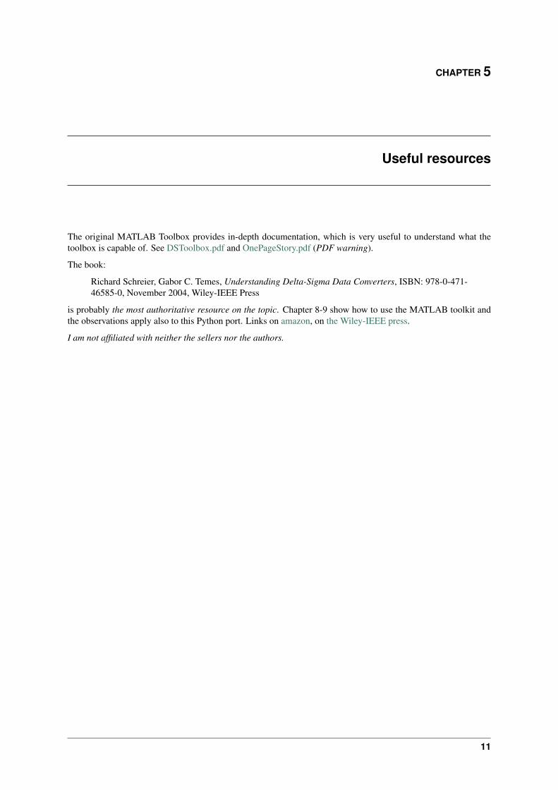
A delta-sigma modulator with a single quantizer is assumed to consist of quantizer connected to a loop filter asshown in the diagram below.

8.1.1 The loop filter

The loop filter is described by an 𝐴𝐵𝐶𝐷 matrix. For single-quantizer systems, the loop filter is a two-input,one-output linear system and 𝐴𝐵𝐶𝐷 is an (𝑛+1, 𝑛+2) matrix, partitioned into 𝐴 (𝑛, 𝑛), 𝐵 (𝑛, 2), 𝐶 (1, 𝑛) and𝐷 (1, 2) sub-matrices as shown below:

𝐴𝐵𝐶𝐷 =

[𝐴 𝐵𝐶 𝐷

].

The equations for updating the state and computing the output of the loop filter are:

𝑥(𝑛+ 1) = 𝐴𝑥(𝑛) +𝐵

[𝑢(𝑛)𝑣(𝑛)

]

𝑦(𝑛) = 𝐶𝑥(𝑛) +𝐷

[𝑢(𝑛)𝑣(𝑛)

].

Where 𝑢(𝑛) is the input sequence and 𝑣(𝑛) is the modulator output sequence.

This formulation is sufficiently general to encompass all single-quantizer modulators which employ linear loopfilters. The toolbox currently supports translation to/from an ABCD descrip- tion and coefficients for the followingtopologies:

• CIFB : Cascade-of-integrators, feedback form.

17

• CIFF : Cascade-of-integrators, feedforward form.

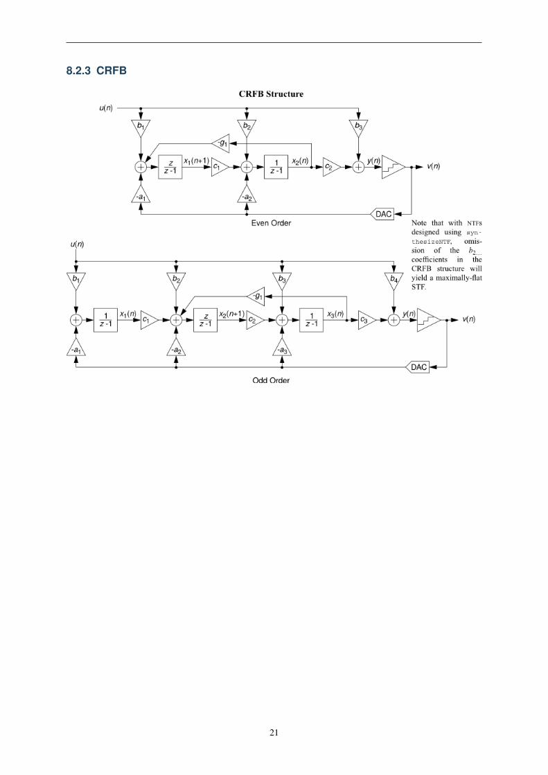
• CRFB : Cascade-of-resonators, feedback form.

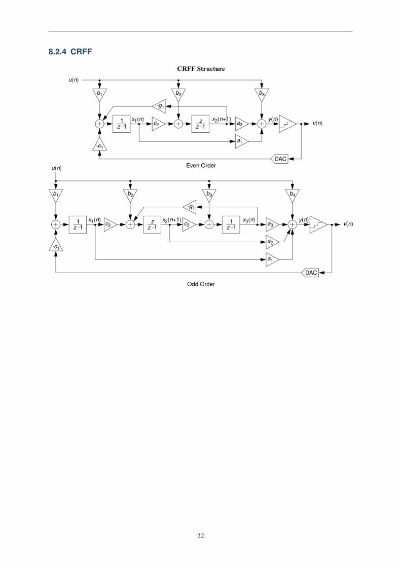
• CRFF : Cascade-of-resonators, feedforward form.

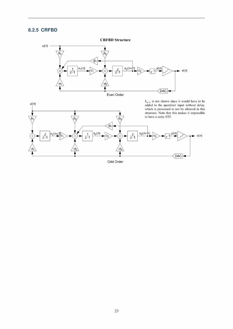
• CRFBD : Cascade-of-resonators, feedback form, delaying quantizer.

• CRFFD : Cascade-of-resonators, feedforward form, delaying quantizer

• PFF : Parallel feed-forward

• Stratos : A CIFF-like structure with non-delaying resonator feedbacks 1

See Topologies diagrams for a block-level view of the different modulator structures.

Multi-input and multi-quantizer systems can also be described with an ABCD matrix and the previous equationwill still apply. For an 𝑛𝑖-input, 𝑛𝑜-output modulator, the dimensions of the sub-matrices are 𝐴: (𝑛, 𝑛), 𝐵:(𝑛, 𝑛𝑖 + 𝑛𝑜), 𝐶: (𝑛𝑜, 𝑛) and 𝐷: (𝑛𝑜, 𝑛𝑖 + 𝑛𝑜).

8.1.2 Quantizer model

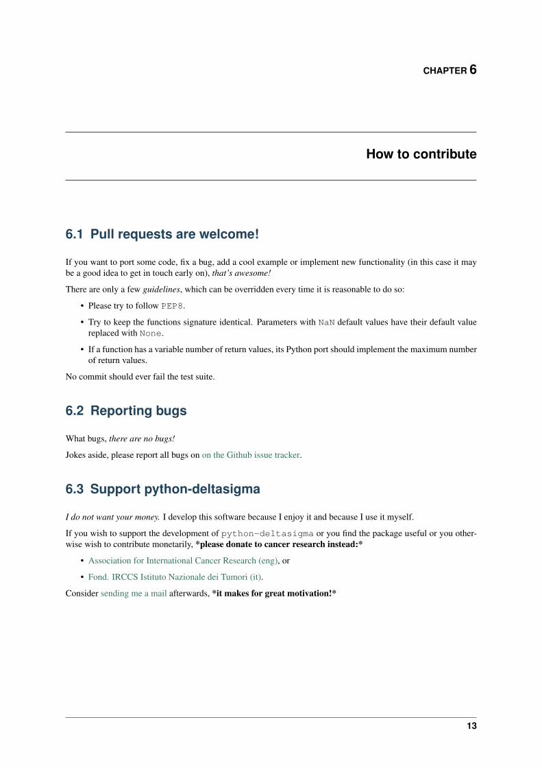
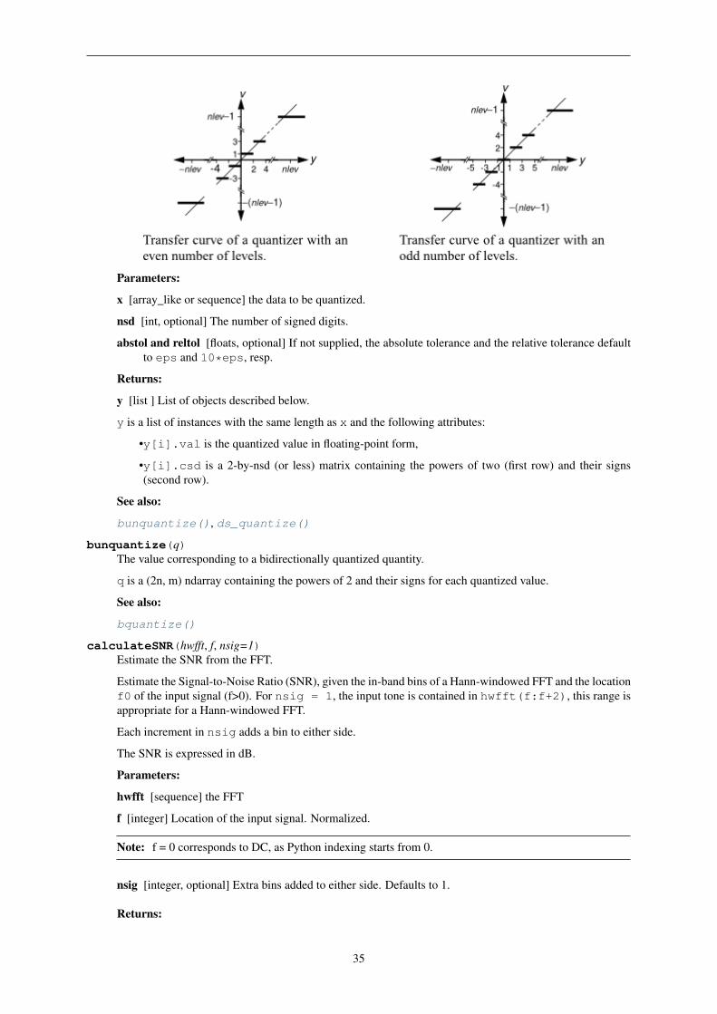
The quantizer is ideal, producing integer outputs centered about zero. Quantizers with an even number of levelsare of the mid-rise type and produce outputs which are odd integers. Quantizers with an odd number of levels areof the mid-tread type and produce outputs which are even inte- gers.

See also:

bquantize(), bunquantize()

8.2 Topologies diagrams

All the following topology diagrams are reproduced from DSToolbox.pdf in the MATLAB Delta Sigma Toolbox,written by Richard Schreier. All credits belong to the original author.

1 Contributed to the MATLAB delta sigma toolbox in 2007 by Jeff Gealow.

18

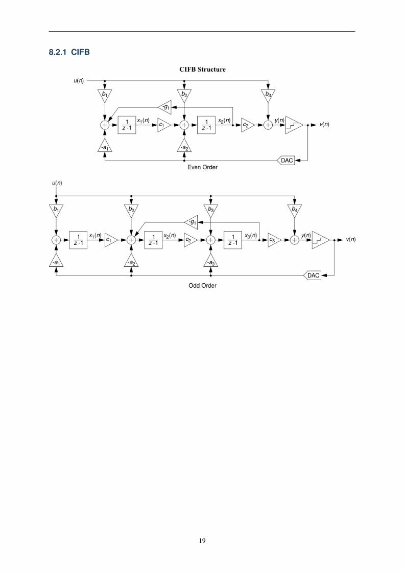
8.2.1 CIFB

19

8.2.2 CIFF

20

8.2.3 CRFB

21

8.2.4 CRFF

22

8.2.5 CRFBD

23

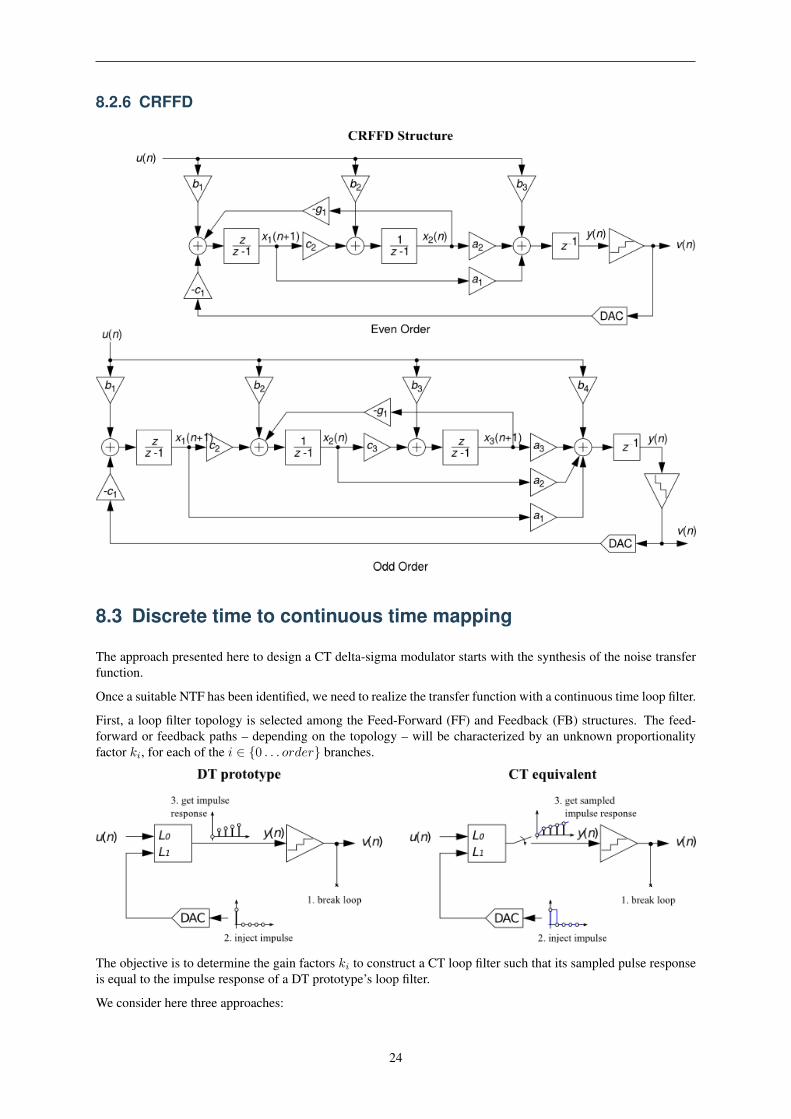
8.2.6 CRFFD

8.3 Discrete time to continuous time mapping

The approach presented here to design a CT delta-sigma modulator starts with the synthesis of the noise transferfunction.

Once a suitable NTF has been identified, we need to realize the transfer function with a continuous time loop filter.

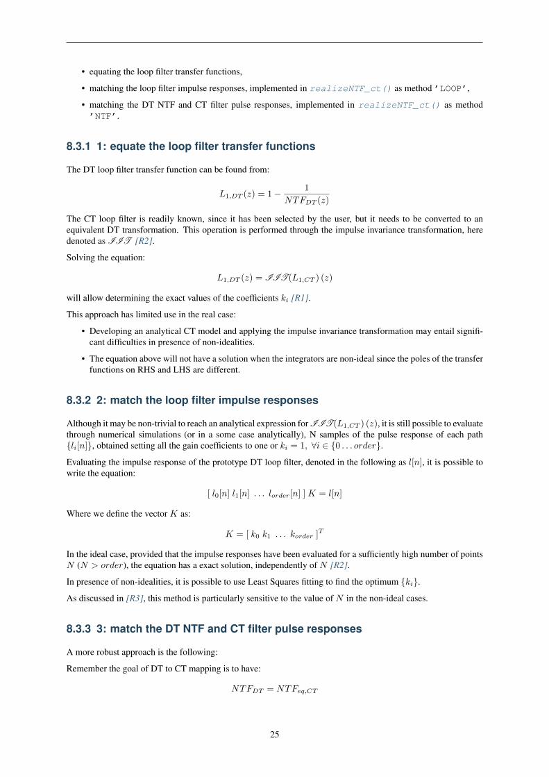
First, a loop filter topology is selected among the Feed-Forward (FF) and Feedback (FB) structures. The feed-forward or feedback paths – depending on the topology – will be characterized by an unknown proportionalityfactor 𝑘𝑖, for each of the 𝑖 ∈ {0 . . . 𝑜𝑟𝑑𝑒𝑟} branches.

The objective is to determine the gain factors 𝑘𝑖 to construct a CT loop filter such that its sampled pulse responseis equal to the impulse response of a DT prototype’s loop filter.

We consider here three approaches:

24

• equating the loop filter transfer functions,

• matching the loop filter impulse responses, implemented in realizeNTF_ct() as method ’LOOP’,

• matching the DT NTF and CT filter pulse responses, implemented in realizeNTF_ct() as method’NTF’.

8.3.1 1: equate the loop filter transfer functions

The DT loop filter transfer function can be found from:

𝐿1,𝐷𝑇 (𝑧) = 1− 1

𝑁𝑇𝐹𝐷𝑇 (𝑧)

The CT loop filter is readily known, since it has been selected by the user, but it needs to be converted to anequivalent DT transformation. This operation is performed through the impulse invariance transformation, heredenoted as IIT [R2].

Solving the equation:

𝐿1,𝐷𝑇 (𝑧) = IIT (𝐿1,𝐶𝑇 ) (𝑧)

will allow determining the exact values of the coefficients 𝑘𝑖 [R1].

This approach has limited use in the real case:

• Developing an analytical CT model and applying the impulse invariance transformation may entail signifi-cant difficulties in presence of non-idealities.

• The equation above will not have a solution when the integrators are non-ideal since the poles of the transferfunctions on RHS and LHS are different.

8.3.2 2: match the loop filter impulse responses

Although it may be non-trivial to reach an analytical expression for IIT (𝐿1,𝐶𝑇 ) (𝑧), it is still possible to evaluatethrough numerical simulations (or in a some case analytically), N samples of the pulse response of each path{𝑙𝑖[𝑛]}, obtained setting all the gain coefficients to one or 𝑘𝑖 = 1, ∀𝑖 ∈ {0 . . . 𝑜𝑟𝑑𝑒𝑟}.

Evaluating the impulse response of the prototype DT loop filter, denoted in the following as 𝑙[𝑛], it is possible towrite the equation:

[ 𝑙0[𝑛] 𝑙1[𝑛] . . . 𝑙𝑜𝑟𝑑𝑒𝑟[𝑛] ]𝐾 = 𝑙[𝑛]

Where we define the vector 𝐾 as:

𝐾 = [ 𝑘0 𝑘1 . . . 𝑘𝑜𝑟𝑑𝑒𝑟 ]𝑇

In the ideal case, provided that the impulse responses have been evaluated for a sufficiently high number of points𝑁 (𝑁 > 𝑜𝑟𝑑𝑒𝑟), the equation has a exact solution, independently of 𝑁 [R2].

In presence of non-idealities, it is possible to use Least Squares fitting to find the optimum {𝑘𝑖}.

As discussed in [R3], this method is particularly sensitive to the value of 𝑁 in the non-ideal cases.

8.3.3 3: match the DT NTF and CT filter pulse responses

A more robust approach is the following:

Remember the goal of DT to CT mapping is to have:

𝑁𝑇𝐹𝐷𝑇 = 𝑁𝑇𝐹𝑒𝑞,𝐶𝑇

25

And by definition:

𝑁𝑇𝐹 =1

1 + 𝐿1(𝑧)

Combining the two we can write the equation:

𝑁𝑇𝐹𝐷𝑇 =1

1 + 𝐿1,𝑒𝑞,𝐶𝑇 (𝑧)

To avoid having to apply the impulse invariance transformation, we can rewrite the above in the time domain,getting: ∑

𝑖

𝑘𝑖 (ℎ[𝑛] * 𝑙𝑖[𝑛]) = 𝛿[𝑛]− ℎ[𝑛] ∀𝑖

Where ℎ[𝑛] is the impulse response of the DT NTF.

The above can be rewritten as:

[ ℎ[𝑛] * 𝑙0[𝑛] . . . ℎ[𝑛] * 𝑙𝑜𝑟𝑑𝑒𝑟[𝑛] ]𝐾 = 𝛿[𝑛]− ℎ[𝑛]

And solved exactly, in the ideal case, or in the least squares sense, in presence of non-idealities [R3].

26

CHAPTER 9

Package contents

9.1 Key Functions

synthesizeNTF() Synthesize a Noise Transfer Function (NTF) for a delta-sigma modulator.clans() Optimal NTF design for a multi-bit modulator.synthesizeChebyshevNTF()Synthesize a noise transfer function for a delta-sigma modulator.simulateDSM() Simulate a delta-sigma modulator.simulateSNR() Determine the SNR for a delta-sigma modulator by using simulations.realizeNTF() Convert an NTF into coefficients for the desired structure.stuffABCD() Calculate the ABCD matrix from the parameters of a modulator topology.mapABCD() Compute the coefficients for a given modulator topology.scaleABCD() Scale the loop filter of a general delta-sigma modulator for dynamic range.calculateTF() Calculate the NTF and STF of a delta-sigma modulator.realizeNTF_ct() Realize an NTF with a continuous-time loop filter.mapCtoD() Map a MIMO continuous-time modulator to an equivalent discrete-time

counterpart.evalTFP() Evaluate a continuous-time - discrete-time transfer function product.

9.2 Functions for quadrature delta-sigma modulators

Several of the previous functions also handle quadrature modulators.

In addition to those, the following are available specifically for quadrature modulators:

synthesizeQNTF() Synthesize a noise transfer function for a quadrature modulator.realizeQNTF() Convert a quadrature NTF into an ABCD matrix.simulateQDSM() Simulate a quadrature Delta-Sigma modulator.simulateQSNR() Determine the SNR for a quadrature delta-sigma modulator using simulations.calculateQTF() Calculate noise and signal transfer functions for a quadrature modulator.mapQtoR() Map a quadrature ABCD matrix to a real one.mapRtoQ() Map a real ABCD matrix to a quadrature one.

9.3 Other selected functions

The following are auxiliary functions that complement the key functions above.

27

mod1() A description of the first-order modulator.mod2() A description of the second-order modulator.calculateSNR() Estimate the SNR from the FFT.predictSNR() Predict the SNR curve of a binary delta-sigma modulator.partitionABCD() Partition ABCD matrix into the state-space matrices A, B, C, D.infnorm() Find the infinity norm of a z-domain transfer function.impL1() Impulse response evaluation for NTFs.l1norm() Compute the l1-norm of a z-domain transfer function.pulse() Calculate the sampled pulse response of a CT system.rmsGain() Compute the root mean-square gain of a discrete-time TF.

9.4 Utility functions for simulation of delta-sigma modulators

Functions for low-level handling of delta-sigma modulator representations, their evaluation and filtering.

bquantize() Bidirectionally quantize a 1D vector x to nsd signed digits.bunquantize() The value corresponding to a bidirectionally quantized quantity.delay() Delay a signal by a give number of samples.ds_f1f2() Get the neighbouring frequencies to the carrier to calculate the SNR.ds_freq() Frequency vector suitable for plotting the frequency response of an NTF.ds_hann() A Hanning (Hann) window of given length.ds_quantize() Quantize a vector.dsclansNTF() Conversion of CLANS parameters into a NTF.evalMixedTF() Evaluate a mixed-signal transfer function.evalRPoly() Compute the value of a polynomial which is given in terms of its roots.evalTF() Evaluate the rational transfer function (TF) at the given z point(s).nabsH() Compute the negative of the absolute value of H.peakSNR() Find the SNR peak by fitting the SNR curve.sinc_decimate() Decimate a vector by a sinc filter of given order and length.zinc() Calculate the magnitude response of a cascade of n m-th order comb filters.

9.5 General utilities for data processing

The following are functions useful for misc. tasks, like manipulating data, conversions or padding, for example.They provide specialty functions which are not otherwise available in the usual scientific Python stack.

circshift() Shift an array circularly.cplxpair() Sort complex roots into complex conjugate pairs.db() Calculate the dB equivalent of a given RMS signal.dbm() Calculate the dBm equivalent of a given RMS voltage.dbp() Calculate the dB equivalent of a given power ratio.dbv() Calculate the dB equivalent of a given voltage ratio.gcd() Calculate the Greatest Common Divisor (GCD) of two integers.lcm() Calculate the Least Common Multiple (LCD) of two integers.mfloor() Round a vector towards -Inf.mround() Round a vector to the nearest integers.padb() Pad a matrix on the bottom to length n with value val.padl() Pad a matrix on the left to length n with value val.padr() Pad a matrix on the right to length n with value val.padt() Pad a matrix on the top to length n with value val.rat() Rational fraction approximation.rms() Calculate the RMS value of x.undbm() Calculate the RMS voltage equivalent to a given power expressed in dBm.undbp() Calculate the power equivalent to a given value in dB.undbv() Calculate the voltage ratio equivalent to a given power expressed in dB.

28

9.6 Plotting and data display utilitites

Graphic functions:

DocumentNTF() Plot the NTF’s poles and zeros as well as its frequency-response.PlotExampleSpectrum() Plot a spectrum suitable to exemplify the NTF performance.axisLabels() Utility function to quickly generate the alphanumeric labels for a plot axis.bilogplot() Plot the spectrum of a band-pass modulator in dB.changeFig() Quickly change several figure parameters.figureMagic() Utility function to quickly set several plot parameters.lollipop() Plot lollipops (o’s and sticks).plotPZ() Plot the poles and zeros of a transfer function.plotSpectrum() Plot a smoothed spectrum on a LOG x-axis.

Textual and non-graphic, display-related functions:

SIunits() Calculates the factor for representing a given value in engineering notation.bplogsmooth() Smooth the FFT and convert it to dB.circ_smooth() Smooth the PSD for linear x-axis plotting.logsmooth() Smooth the FFT, and convert it to dB.pretty_lti() A pretty representation of a TF, suitable for printing to screen.

29

30

CHAPTER 10

All functions in alphabetical order

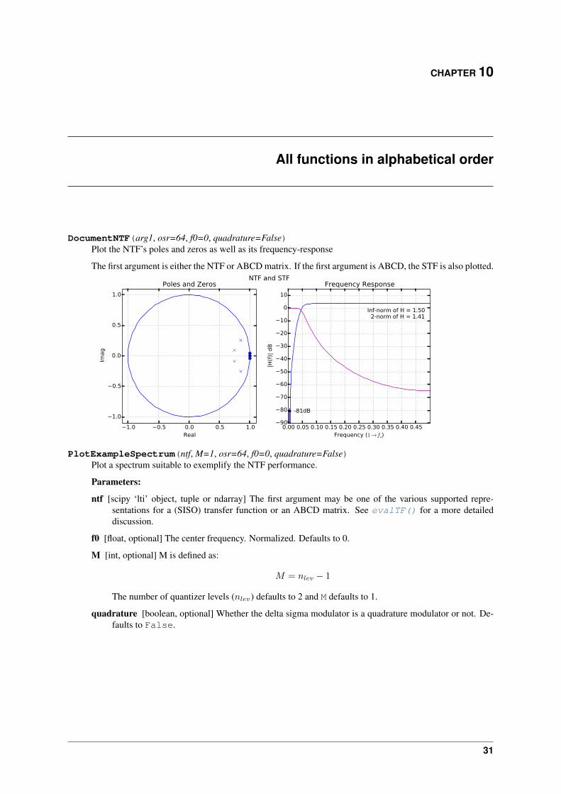
DocumentNTF(arg1, osr=64, f0=0, quadrature=False)Plot the NTF’s poles and zeros as well as its frequency-response

The first argument is either the NTF or ABCD matrix. If the first argument is ABCD, the STF is also plotted.

1.0 0.5 0.0 0.5 1.0Real

1.0

0.5

0.0

0.5

1.0

Imag

Poles and Zeros

0.00 0.05 0.10 0.15 0.20 0.25 0.30 0.35 0.40 0.45Frequency (1→fs)

90

80

70

60

50

40

30

20

10

0

10

|H(f)

| dB

-81dB

Inf-norm of H = 1.50 2-norm of H = 1.41

Frequency ResponseNTF and STF

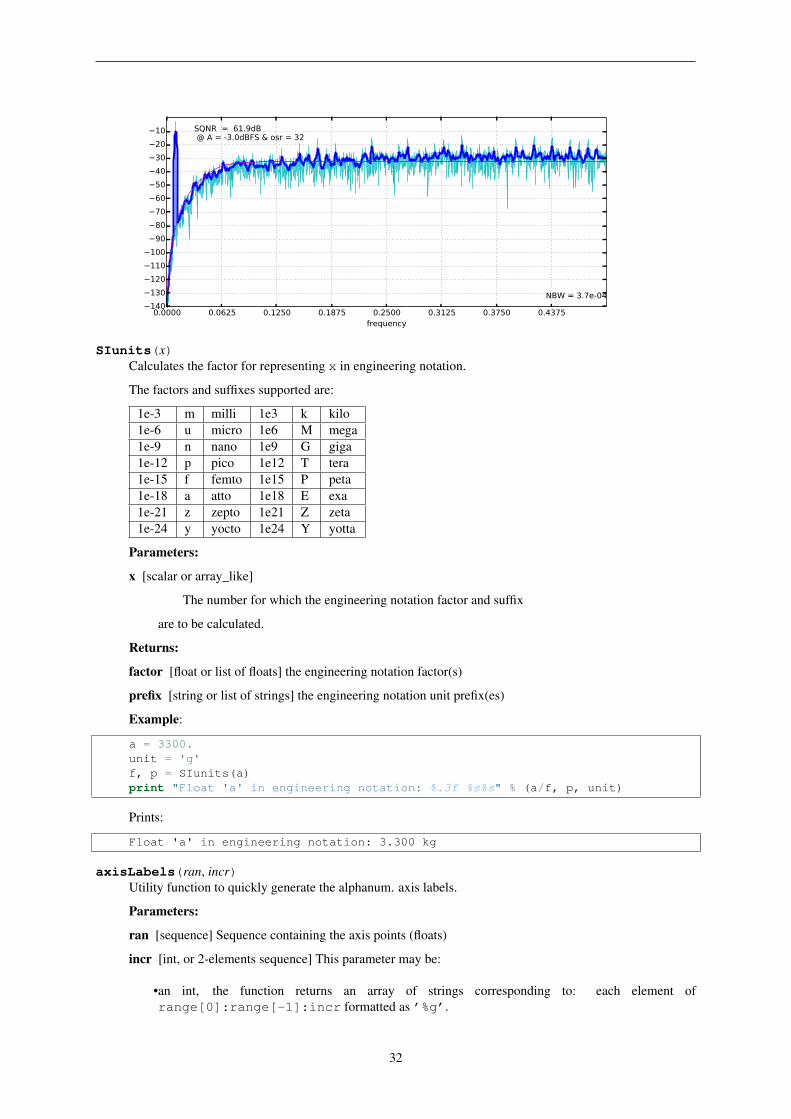
PlotExampleSpectrum(ntf, M=1, osr=64, f0=0, quadrature=False)Plot a spectrum suitable to exemplify the NTF performance.

Parameters:

ntf [scipy ‘lti’ object, tuple or ndarray] The first argument may be one of the various supported repre-sentations for a (SISO) transfer function or an ABCD matrix. See evalTF() for a more detaileddiscussion.

f0 [float, optional] The center frequency. Normalized. Defaults to 0.

M [int, optional] M is defined as:

𝑀 = 𝑛𝑙𝑒𝑣 − 1

The number of quantizer levels (𝑛𝑙𝑒𝑣) defaults to 2 and M defaults to 1.

quadrature [boolean, optional] Whether the delta sigma modulator is a quadrature modulator or not. De-faults to False.

31

0.0000 0.0625 0.1250 0.1875 0.2500 0.3125 0.3750 0.4375frequency

140130120110100

908070605040302010 SQNR = 61.9dB

@ A = -3.0dBFS & osr = 32

NBW = 3.7e-04

SIunits(x)Calculates the factor for representing x in engineering notation.

The factors and suffixes supported are:

1e-3 m milli 1e3 k kilo1e-6 u micro 1e6 M mega1e-9 n nano 1e9 G giga1e-12 p pico 1e12 T tera1e-15 f femto 1e15 P peta1e-18 a atto 1e18 E exa1e-21 z zepto 1e21 Z zeta1e-24 y yocto 1e24 Y yotta

Parameters:

x [scalar or array_like]

The number for which the engineering notation factor and suffix

are to be calculated.

Returns:

factor [float or list of floats] the engineering notation factor(s)

prefix [string or list of strings] the engineering notation unit prefix(es)

Example:

a = 3300.unit = 'g'f, p = SIunits(a)print "Float 'a' in engineering notation: %.3f %s%s" % (a/f, p, unit)

Prints:

Float 'a' in engineering notation: 3.300 kg

axisLabels(ran, incr)Utility function to quickly generate the alphanum. axis labels.

Parameters:

ran [sequence] Sequence containing the axis points (floats)

incr [int, or 2-elements sequence] This parameter may be:

•an int, the function returns an array of strings corresponding to: each element ofrange[0]:range[-1]:incr formatted as ’%g’.

32

•a list, the function returns an array of strings corresponding to: each element ofincr[1]:range[-1]:incr[0] formatted as ’%g’.

Note: All elements in ran less than 1e-6 are rounded down to 0.

Returns:

labels : list of strings

Raises:

ValueError: “Unrecognised incr.”

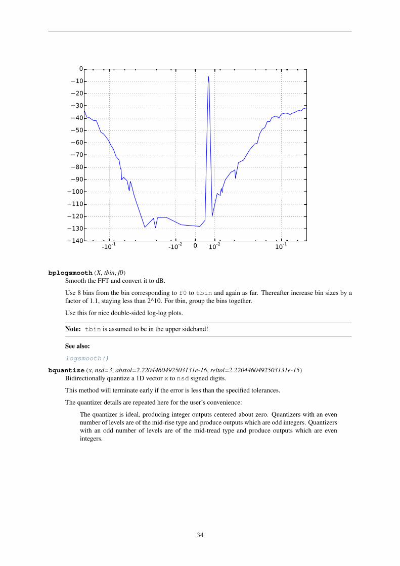
bilogplot(V, f0, fbin, x, y, **fmt)Plot the spectrum of a band-pass modulator in dB.

The plot is a logarithmic plot, centered in 0, corresponding to f0, extending to negative frequencies, withrespect to the center frequencies and to positive frequencies.

The plot employs a logarithmic x-axis transform far from the origin and a linear one close to it, allowing thex-axis to reach zero and extend to negative values as well.

Note: This is implemented in a slightly different way from The MATLAB Delta Sigma Toolbox, whereall values below xmin are clipped and the scale is always logarithmic. It our implementation, no clippin isdone and below xmin the data is simply plotted with a linear scale. For this reason slightly different plotsmay be generated.

Parameters:

V [1d-ndarray or sequence] Hann-windowed FFT

f0 [int] Bin number of center frequency

fbin [int] Bin number of test tone

x [3-elements sequence-like] x is a sequence of three positive floats: xmin, xmax_left, xmax_right.xmin is the minimum value of the logarithmic plot range. xmax_left is the length of the plottinginterval on the left (negative) side, xmax_right is its respective on the right (positive) side.

y [3-elements sequence-like] y is a sequence of three floats: ymin, ymax, dy. ymin is the minimum valueof the y-axis, ymax its maximum value and dy is the ticks spacing.

Note: The MATLAB Delta Sigma toolbox allows for a fourth option y_skip, which is the incr valuepassed to MATLAB’s axisLabels. No such thing is supported here. A warning is issued if len(v) ==4.

Additional keyword parameters **fmt will be passed to matplotlib’s semilogx().

The FFT is smoothed before plotting and converted to dB. See logsmooth() for details regarding thealgorithm used.

Returns:

None

33

-10-1 -10-2 0 10-2 10-1140

130

120

110

100

90

80

70

60

50

40

30

20

10

0

bplogsmooth(X, tbin, f0)Smooth the FFT and convert it to dB.

Use 8 bins from the bin corresponding to f0 to tbin and again as far. Thereafter increase bin sizes by afactor of 1.1, staying less than 2^10. For tbin, group the bins together.

Use this for nice double-sided log-log plots.

Note: tbin is assumed to be in the upper sideband!

See also:

logsmooth()

bquantize(x, nsd=3, abstol=2.2204460492503131e-16, reltol=2.2204460492503131e-15)Bidirectionally quantize a 1D vector x to nsd signed digits.

This method will terminate early if the error is less than the specified tolerances.

The quantizer details are repeated here for the user’s convenience:

The quantizer is ideal, producing integer outputs centered about zero. Quantizers with an evennumber of levels are of the mid-rise type and produce outputs which are odd integers. Quantizerswith an odd number of levels are of the mid-tread type and produce outputs which are evenintegers.

34

Parameters:

x [array_like or sequence] the data to be quantized.

nsd [int, optional] The number of signed digits.

abstol and reltol [floats, optional] If not supplied, the absolute tolerance and the relative tolerance defaultto eps and 10*eps, resp.

Returns:

y [list ] List of objects described below.

y is a list of instances with the same length as x and the following attributes:

•y[i].val is the quantized value in floating-point form,

•y[i].csd is a 2-by-nsd (or less) matrix containing the powers of two (first row) and their signs(second row).

See also:

bunquantize(), ds_quantize()

bunquantize(q)The value corresponding to a bidirectionally quantized quantity.

q is a (2n, m) ndarray containing the powers of 2 and their signs for each quantized value.

See also:

bquantize()

calculateSNR(hwfft, f, nsig=1)Estimate the SNR from the FFT.

Estimate the Signal-to-Noise Ratio (SNR), given the in-band bins of a Hann-windowed FFT and the locationf0 of the input signal (f>0). For nsig = 1, the input tone is contained in hwfft(f:f+2), this range isappropriate for a Hann-windowed FFT.

Each increment in nsig adds a bin to either side.

The SNR is expressed in dB.

Parameters:

hwfft [sequence] the FFT

f [integer] Location of the input signal. Normalized.

Note: f = 0 corresponds to DC, as Python indexing starts from 0.

nsig [integer, optional] Extra bins added to either side. Defaults to 1.

Returns:

35

SNR [scalar] The computed SNR value in dB.

calculateTF(ABCD, k=1.0)Calculate the NTF and STF of a delta-sigma modulator.

The calculation is performed for a given loop filter ABCD matrix, assuming a quantizer gain of k.

Parameters:

ABCD [array_like,] The ABCD matrix that describes the system.

k [float or ndarray-like, optional] The quantizer gains. If only one quantizer is present, it may be set toa float, corresponding to the quantizer gain. If multiple quantizers are present, a list should be used,with quantizer gains ordered according to the order in which the quantizer inputs apperar in the C andD submatrices. If not specified, a default of one quatizer with gain 1. is assumed.

Returns:

(NTF, STF) : a tuple of two LTI objects (or of two lists of LTI objects).

If the system has multiple quantizers, multiple STFs and NTFs will be returned.

In that case:

•STF[i] is the STF from u to output number i.

•NTF[i, j] is the NTF from the quantization noise of the quantizer number j to output number i.

Note:

Setting k to a list is unsupported in the MATLAB code (last checked Nov. 2014).

Example:

Realize a fifth-order modulator with the cascade-of-resonators structure, feedback form. Calculate theABCD matrix of the loop filter and verify that the NTF and STF are correct.

from deltasigma import *H = synthesizeNTF(5, 32, 1)a, g, b, c = realizeNTF(H)ABCD = stuffABCD(a,g,b,c)ntf, stf = calculateTF(ABCD)

From which we get:

H:

(z -1) (z^2 -1.997z +1) (z^2 -1.992z +0.9999)--------------------------------------------------------(z -0.7778) (z^2 -1.796z +0.8549) (z^2 -1.613z +0.665)

coefficients:

a: 0.0007, 0.0084, 0.055, 0.2443, 0.5579g: 0.0028, 0.0079b: 0.0007, 0.0084, 0.055, 0.2443, 0.5579, 1.0c: 1.0, 1.0, 1.0, 1.0, 1.0

ABCD matrix:

[[ 1.00000000e+00 0.00000000e+00 0.00000000e+00 0.00000000e+000.00000000e+00 6.75559806e-04 -6.75559806e-04]

[ 1.00000000e+00 1.00000000e+00 -2.79396240e-03 0.00000000e+000.00000000e+00 8.37752565e-03 -8.37752565e-03]

[ 1.00000000e+00 1.00000000e+00 9.97206038e-01 0.00000000e+000.00000000e+00 6.33294166e-02 -6.33294166e-02]

[ 0.00000000e+00 0.00000000e+00 1.00000000e+00 1.00000000e+00-7.90937431e-03 2.44344030e-01 -2.44344030e-01]

[ 0.00000000e+00 0.00000000e+00 1.00000000e+00 1.00000000e+009.92090626e-01 8.02273699e-01 -8.02273699e-01]

36

[ 0.00000000e+00 0.00000000e+00 0.00000000e+00 0.00000000e+001.00000000e+00 1.00000000e+00 0.00000000e+00]]

NTF:

(z -1) (z^2 -1.997z +1) (z^2 -1.992z +0.9999)--------------------------------------------------------(z -0.7778) (z^2 -1.796z +0.8549) (z^2 -1.613z +0.665)

STF:

1

calculateQTF(ABCDr)Calculate noise and signal transfer functions for a quadrature modulator

Parameters:

ABCDr [ndarray] The ABCD matrix, in real form. You may call mapQtoR() to convert an imaginary(quadrature) ABCD matrix to a real one.

Returns:

ntf, stf, intf, istf [tuple of zpk tuples] The quadrature noise and signal transfer functions.

Raises RuntimeError if the supplied ABCD matrix results in denominator mismatches.

cancelPZ(arg1, tol=1e-06)Cancel zeros/poles in a SISO transfer function.

Parameters:

arg1 [LTI system description] Multiple descriptions are supported for the LTI system.

If one argument is used, it is a scipy lti object.

If more arguments are used, they should be arranged in a tuple, the following gives the number ofelements in the tuple and their interpretation:

• 2: (numerator, denominator)

• 3: (zeros, poles, gain)

• 4: (A, B, C, D)

Each argument can be an array or sequence.

tol [float, optional] the absolute tolerance for pole, zero cancellation. Defaults to 1e-6.

Returns:

(z, p, k) [tuple] A tuple containing zeros, poles and gain (unchanged) after poles, zeros cancellation.

changeFig(fontsize=None, linewidth=None, markersize=None, xfticks=False, yfticks=False, bw=False,fig=None)

Quickly change several figure parameters.

Take each axes in the figure, and for each line and text item in the axes, set linewidth, markersize and fontsize.

Parameters:

fontsize [scalar, optional] the font size, given in points, defaults to None, no change.

linewidth [scalar, optional] the line width, given in points. Defaults to None, no change.

markersize [scalar, optional] the marker size, given in points. Defaults to None, no change.

37

xfticks [string, optional] this parameter may be set to ’sci’ or ’plain’ and only has an effect on linearaxes.

If set to ’sci’, the x-axis labels will be formatted in scientific notation, with three decimals, eg’1.000E3’. If set to plain, plain float formatting will be used, eg. ’0.001’.

Defaults to None, meaning no change is performed.

yfticks [string, optional] this parameter may be set to ’sci’ or ’plain’ and only has an effect on linearaxes.

If set to ’sci’, the y-axis labels will be formatted in scientific notation, with three decimals, eg’1.000E3’. If set to plain, plain float formatting will be used, eg. ’0.001’.

Defaults to None, meaning no change is performed.

bw [boolean, optional] if set to True, the figure will be converted to BW. Defaults to False.

fig [a matplotlib figure object, optional] the figure to apply the modifications to, if not given, it is assumedto be the currently active figure.

Returns:

None.

Note: This function may be useful to enhance the readibility of figures to be used in presentations.

See also:

figureMagic(), to quickly change plot ranges and more.

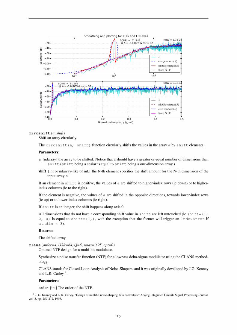
circ_smooth(x, n=16)Smoothing of the PSD x for linear x-axis plotting.

Parameters:

x [1D ndarray] The PSD to be smoothed, or equivalently

𝑥 = |FFT (𝑢(𝑡)) (𝑓)|2

n [int, even, optional] The length of the Hann window used in the smoothing algorithm.

Returns:

y [1D ndarray] The smoothed PSD

See also:

logsmooth(), smoothing algorithm suitable for logarithmic x-axis plotting.

For a comparison of circ_smooth() and logsmooth() (accessed through the helper functionplotSpectrum()) see the following plot.

38

10-3 10-2 10-1140

120

100

80

60

40

20Sp

ectr

um [d

B]SQNR = 61.9dB @ A = -3.0dBFS & osr = 32

NBW = 3.7e-04 Smoothing and plotting for LOG and LIN axes

S

circ_smooth(S)

plotSpectrum(S)

from NTF

0.0 0.1 0.2 0.3 0.4 0.5Normalized frequency (fs →1)

140

120

100

80

60

40

20

Spec

trum

[dB]

SQNR = 61.9dB @ A = -3.0dBFS & osr = 32

NBW = 3.7e-04

S

plotSpectrum(S)

circ_smooth(S)

from NTF

circshift(a, shift)Shift an array circularly.

The circshift(a, shift) function circularly shifts the values in the array a by shift elements.

Parameters:

a [ndarray] the array to be shifted. Notice that a should have a greater or equal number of dimensions thanshift (shift being a scalar is equal to shift being a one-dimension array.)

shift [int or ndarray-like of int.] the N-th element specifies the shift amount for the N-th dimension of theinput array a.

If an element in shift is positive, the values of a are shifted to higher-index rows (ie down) or to higher-index columns (ie to the right).

If the element is negative, the values of a are shifted in the opposite directions, towards lower-index rows(ie up) or to lower-index columns (ie right).

If shift is an integer, the shift happens along axis 0.

All dimensions that do not have a corresponding shift value in shift are left untouched (ie shift=(1,0, 0) is equal to shift=(1,), with the exception that the former will trigger an IndexError ifa.ndim < 3).

Returns:

The shifted array.

clans(order=4, OSR=64, Q=5, rmax=0.95, opt=0)Optimal NTF design for a multi-bit modulator.

Synthesize a noise transfer function (NTF) for a lowpass delta-sigma modulator using the CLANS method-ology.

CLANS stands for Closed-Loop Analysis of Noise-Shapers, and it was originally developed by J.G. Kenneyand L.R. Carley 1.

Parameters:

order [int] The order of the NTF.1 J. G. Kenney and L. R. Carley, “Design of multibit noise-shaping data converters,” Analog Integrated Circuits Signal Processing Journal,

vol. 3, pp. 259-272, 1993.

39

OSR [int] The oversampling ratio.

Q [int] The maximum number of quantization levels used by the fed-back quantization noise. (Mathemat-ically, 𝑄 = ‖ℎ‖1 − 1, i.e. the sum of the absolute values of the impulse response samples minus oneis the maximum instantaneous noise gain.)

rmax [float] The maximum radius for the NTF poles.

opt [int] A flag used to request optimized NTF zeros.

•opt=0 puts all NTF zeros at band center (DC for lowpass modulators).

•opt=1 optimizes the NTF zeros.

•For even-order modulators, opt=2 puts two zeros at band-center, but optimizes the rest.

Returns

ntf [tuple] The modulator NTF, given in ZPK (zero-pole-gain) form.

Example:

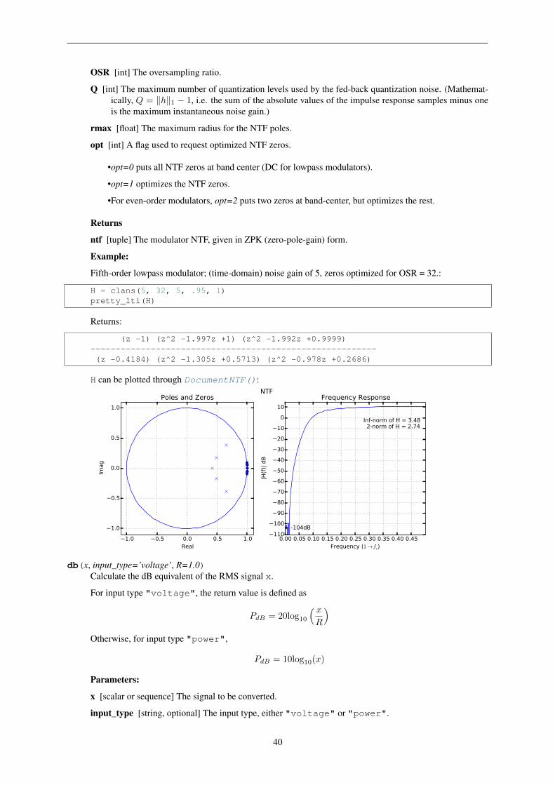
Fifth-order lowpass modulator; (time-domain) noise gain of 5, zeros optimized for OSR = 32.:

H = clans(5, 32, 5, .95, 1)pretty_lti(H)

Returns:

(z -1) (z^2 -1.997z +1) (z^2 -1.992z +0.9999)---------------------------------------------------------(z -0.4184) (z^2 -1.305z +0.5713) (z^2 -0.978z +0.2686)

H can be plotted through DocumentNTF():

1.0 0.5 0.0 0.5 1.0Real

1.0

0.5

0.0

0.5

1.0

Imag

Poles and Zeros

0.00 0.05 0.10 0.15 0.20 0.25 0.30 0.35 0.40 0.45Frequency (1→fs)

110100

9080706050403020100

10

|H(f)

| dB

-104dB

Inf-norm of H = 3.48 2-norm of H = 2.74

Frequency ResponseNTF

db(x, input_type=’voltage’, R=1.0)Calculate the dB equivalent of the RMS signal x.

For input type "voltage", the return value is defined as

𝑃𝑑𝐵 = 20log10

( 𝑥

𝑅

)Otherwise, for input type "power",

𝑃𝑑𝐵 = 10log10(𝑥)

Parameters:

x [scalar or sequence] The signal to be converted.

input_type [string, optional] The input type, either "voltage" or "power".

40

R [float, optional] The normalization resistor value, used only for voltage inputs.

Returns:

PdB [scalar or sequence] The input expressed in dB.

Note: MATLAB provides a function with this exact signature.

See also:

undbm(), undbv(), undbp(), dbv(), dbp(), dbv()

dbm(v, R=50)Calculate the dBm equivalent of an RMS voltage v.

𝑃𝑑𝐵𝑚 = 10log10(1000𝑣2

𝑅)

Parameters:

v [scalar or sequence] The voltages to be converted.

R [scalar, optional] The resistor value the power is calculated upon, defaults to 50 ohm.

Returns:

PdBm [scalar or sequence] The input in dBm.

See also:

undbm(), db(), dbp(), dbv()

dbp(x)Calculate the dB equivalent of the power ratio x.

𝑃𝑑𝐵 = 10log10(𝑥)

Parameters:

x [scalar or sequence] The power ratio to be converted.

Returns:

PdB [scalar or sequence] The input expressed in dB.

See also:

undbp(), db(), dbm(), dbv()

dbv(x)Calculate the dB equivalent of the voltage ratio x.

𝐺𝑑𝐵 = 20log10(|𝑥|)

Parameters:

x [scalar or sequence] The voltage (ratio) to be converted.

Returns:

GdB [scalar or sequence] The input voltage (ratio) expressed in dB.

See also:

undbv(), db(), dbp(), dbm()

delay(x, n=1)Delay signal x by n samples.

ds_f1f2(OSR=64, f0=0.0, complex_flag=False)[f1, f2] = ds_f1f2(OSR=64, f0=0, complex_flag=0) This function has no original docstring.

41

ds_freq(osr=64.0, f0=0.0, quadrature=False)Frequency vector suitable for plotting the frequency response of an NTF

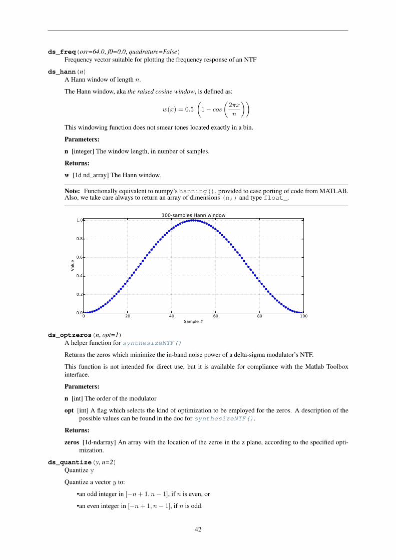
ds_hann(n)A Hann window of length 𝑛.

The Hann window, aka the raised cosine window, is defined as:

𝑤(𝑥) = 0.5

(1− 𝑐𝑜𝑠

(2𝜋𝑥

𝑛

))This windowing function does not smear tones located exactly in a bin.

Parameters:

n [integer] The window length, in number of samples.

Returns:

w [1d nd_array] The Hann window.

Note: Functionally equivalent to numpy’s hanning(), provided to ease porting of code from MATLAB.Also, we take care always to return an array of dimensions (n,) and type float_.

0 20 40 60 80 100Sample #

0.0

0.2

0.4

0.6

0.8

1.0

Valu

e

100-samples Hann window

ds_optzeros(n, opt=1)A helper function for synthesizeNTF()

Returns the zeros which minimize the in-band noise power of a delta-sigma modulator’s NTF.

This function is not intended for direct use, but it is available for compliance with the Matlab Toolboxinterface.

Parameters:

n [int] The order of the modulator

opt [int] A flag which selects the kind of optimization to be employed for the zeros. A description of thepossible values can be found in the doc for synthesizeNTF().

Returns:

zeros [1d-ndarray] An array with the location of the zeros in the z plane, according to the specified opti-mization.

ds_quantize(y, n=2)Quantize y

Quantize a vector 𝑦 to:

•an odd integer in [−𝑛+ 1, 𝑛− 1], if 𝑛 is even, or

•an even integer in [−𝑛+ 1, 𝑛− 1], if 𝑛 is odd.

42

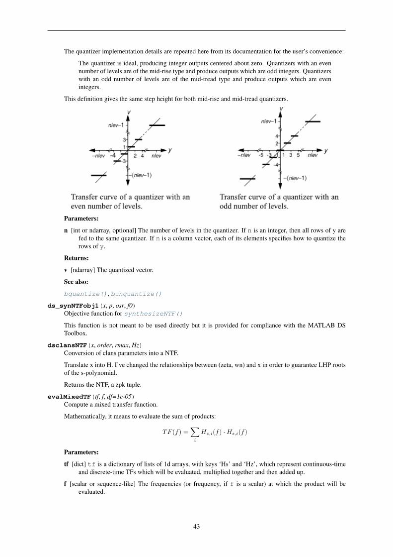
The quantizer implementation details are repeated here from its documentation for the user’s convenience:

The quantizer is ideal, producing integer outputs centered about zero. Quantizers with an evennumber of levels are of the mid-rise type and produce outputs which are odd integers. Quantizerswith an odd number of levels are of the mid-tread type and produce outputs which are evenintegers.

This definition gives the same step height for both mid-rise and mid-tread quantizers.

Parameters:

n [int or ndarray, optional] The number of levels in the quantizer. If n is an integer, then all rows of y arefed to the same quantizer. If n is a column vector, each of its elements specifies how to quantize therows of y.

Returns:

v [ndarray] The quantized vector.

See also:

bquantize(), bunquantize()

ds_synNTFobj1(x, p, osr, f0)Objective function for synthesizeNTF()

This function is not meant to be used directly but it is provided for compliance with the MATLAB DSToolbox.

dsclansNTF(x, order, rmax, Hz)Conversion of clans parameters into a NTF.

Translate x into H. I’ve changed the relationships between (zeta, wn) and x in order to guarantee LHP rootsof the s-polynomial.

Returns the NTF, a zpk tuple.

evalMixedTF(tf, f, df=1e-05)Compute a mixed transfer function.

Mathematically, it means to evaluate the sum of products:

𝑇𝐹 (𝑓) =∑𝑖

𝐻𝑧,𝑖(𝑓) ·𝐻𝑠,𝑖(𝑓)

Parameters:

tf [dict] tf is a dictionary of lists of 1d arrays, with keys ‘Hs’ and ‘Hz’, which represent continuous-timeand discrete-time TFs which will be evaluated, multiplied together and then added up.

f [scalar or sequence-like] The frequencies (or frequency, if f is a scalar) at which the product will beevaluated.

43

df [float, optional] If the method happens to evaluate a transfer function in a root, it will move away of df,defaulting to 1E-5.

Returns:

TF [scalar or sequence] The sum of products computed at f.

evalRPoly(roots, x, k=1)Compute the value of a polynomial which is given in terms of its roots.

evalTF(tf, z)Evaluates the rational function tf at the point(s) given in z.

Parameters:

tf [object] the LTI description of the CT system, which can be in one of the following forms:

•an LTI object,

•a zpk tuple,

•a (num, den) tuple,

•an ABCD matrix (internally converted to zpk representation),

•a list-like containing the A, B, C, D matrices (also internally converted to zpk representation).

z [scalar or 1d ndarray] The z values for which tf is to be evaluated.

Returns:

tf(z) [scalar or 1d-ndarray] The result.

evalTFP(Hs, Hz, f)Evaluate a CT-DT transfer function product.

Compute the value of a transfer function product Hs*Hz at a frequency f, where Hs is a continuous-time TFand Hz is a discrete-time TF.

Use this function to evaluate the signal transfer function of a continuous-time (CT) system. In this contextHs is the open-loop response of the loop filter from the u input and Hz is the closed-loop noise transferfunction.

Note: This function attempts to cancel poles in Hs with zeros in Hz.

Parameters:

Hs [tuple] Hs is a CT (SISO) TF in zpk-tuple form.

Hz [tuple] Hz is a DT (SISO) TF in zpk-tuple form.

f [scalar or 1D array or sequence] Frequency values.

Returns:

H [scalar, or ndarray or sequence] The calculated values:

𝐻(𝑓) = 𝐻𝑠(𝑗2𝜋𝑓) 𝐻𝑧(𝑒𝑗2𝜋𝑓 )

H has the same form as f.

See also:

evalMixedTF(), a more advanced version of this function which is used to evaluate the individual feed-in transfer functions of a CT modulator.

Example:

Plot the STF of the 2nd-order CT system depicted at mapCtoD().:

44

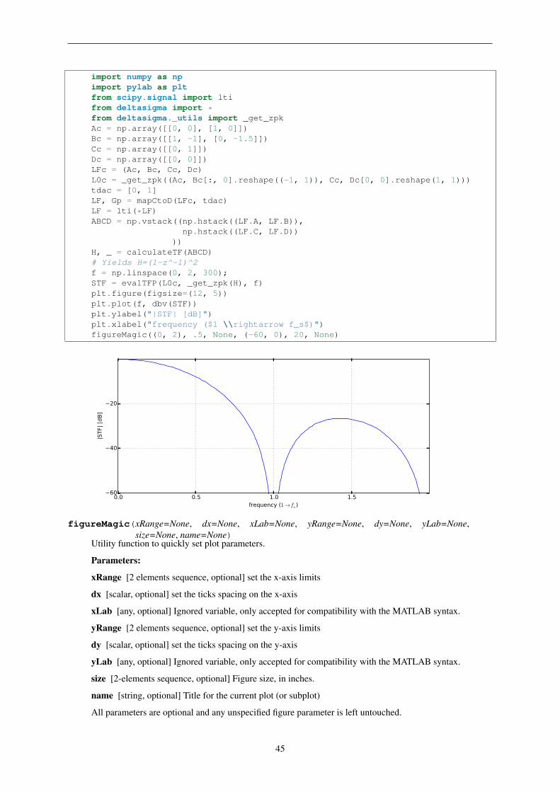
import numpy as npimport pylab as pltfrom scipy.signal import ltifrom deltasigma import *from deltasigma._utils import _get_zpkAc = np.array([[0, 0], [1, 0]])Bc = np.array([[1, -1], [0, -1.5]])Cc = np.array([[0, 1]])Dc = np.array([[0, 0]])LFc = (Ac, Bc, Cc, Dc)L0c = _get_zpk((Ac, Bc[:, 0].reshape((-1, 1)), Cc, Dc[0, 0].reshape(1, 1)))tdac = [0, 1]LF, Gp = mapCtoD(LFc, tdac)LF = lti(*LF)ABCD = np.vstack((np.hstack((LF.A, LF.B)),

np.hstack((LF.C, LF.D))))

H, _ = calculateTF(ABCD)# Yields H=(1-z^-1)^2f = np.linspace(0, 2, 300);STF = evalTFP(L0c, _get_zpk(H), f)plt.figure(figsize=(12, 5))plt.plot(f, dbv(STF))plt.ylabel("|STF| [dB]")plt.xlabel("frequency ($1 \\rightarrow f_s$)")figureMagic((0, 2), .5, None, (-60, 0), 20, None)

0.0 0.5 1.0 1.5frequency (1→fs )

60

40

20

|STF

| [dB

]

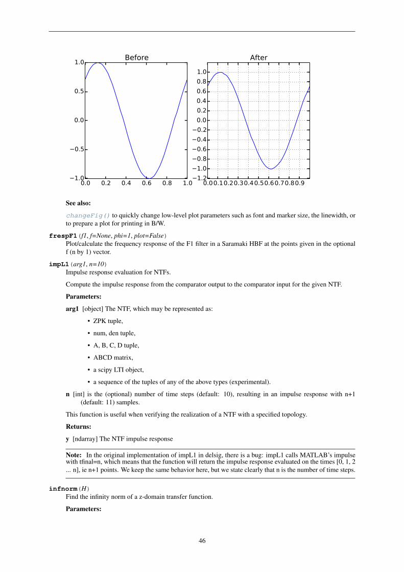
figureMagic(xRange=None, dx=None, xLab=None, yRange=None, dy=None, yLab=None,size=None, name=None)

Utility function to quickly set plot parameters.

Parameters:

xRange [2 elements sequence, optional] set the x-axis limits

dx [scalar, optional] set the ticks spacing on the x-axis

xLab [any, optional] Ignored variable, only accepted for compatibility with the MATLAB syntax.

yRange [2 elements sequence, optional] set the y-axis limits

dy [scalar, optional] set the ticks spacing on the y-axis

yLab [any, optional] Ignored variable, only accepted for compatibility with the MATLAB syntax.

size [2-elements sequence, optional] Figure size, in inches.

name [string, optional] Title for the current plot (or subplot)

All parameters are optional and any unspecified figure parameter is left untouched.

45

0.0 0.2 0.4 0.6 0.8 1.01.0

0.5

0.0

0.5

1.0 Before

0.00.10.20.30.40.50.60.70.80.91.21.00.80.60.40.20.00.20.40.60.81.0

After

See also:

changeFig() to quickly change low-level plot parameters such as font and marker size, the linewidth, orto prepare a plot for printing in B/W.

frespF1(f1, f=None, phi=1, plot=False)Plot/calculate the frequency response of the F1 filter in a Saramaki HBF at the points given in the optionalf (n by 1) vector.

impL1(arg1, n=10)Impulse response evaluation for NTFs.

Compute the impulse response from the comparator output to the comparator input for the given NTF.

Parameters:

arg1 [object] The NTF, which may be represented as:

• ZPK tuple,

• num, den tuple,

• A, B, C, D tuple,

• ABCD matrix,

• a scipy LTI object,

• a sequence of the tuples of any of the above types (experimental).

n [int] is the (optional) number of time steps (default: 10), resulting in an impulse response with n+1(default: 11) samples.

This function is useful when verifying the realization of a NTF with a specified topology.

Returns:

y [ndarray] The NTF impulse response

Note: In the original implementation of impL1 in delsig, there is a bug: impL1 calls MATLAB’s impulsewith tfinal=n, which means that the function will return the impulse response evaluated on the times [0, 1, 2... n], ie n+1 points. We keep the same behavior here, but we state clearly that n is the number of time steps.

infnorm(H)Find the infinity norm of a z-domain transfer function.

Parameters:

46

H [object] the LTI description of the DT system, which can be in one of the following forms:

• an LTI object,

• a zpk tuple,

• a (num, den) tuple,

• an ABCD matrix (internally converted to zpk representation),

• a list-like containing the A, B, C, D matrices (also internally converted to zpk representation).

Returns:

Hinf [float] The infinity norm of H.

fmax [float] The frequency to which Hinf corresponds.

l1norm(H)Compute the l1-norm of a z-domain transfer function.

The norm is evaluated over the first 100 samples.

Parameters:

H [sequence or lti object] Any supported LTI representation is accepted.

Returns:

l1normH [float] The L1 norm of H.

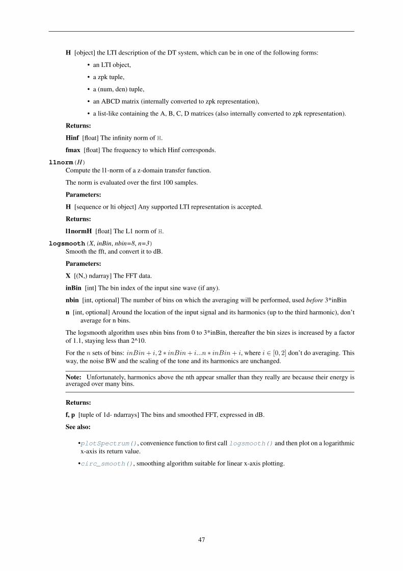
logsmooth(X, inBin, nbin=8, n=3)Smooth the fft, and convert it to dB.

Parameters:

X [(N,) ndarray] The FFT data.

inBin [int] The bin index of the input sine wave (if any).

nbin [int, optional] The number of bins on which the averaging will be performed, used before 3*inBin

n [int, optional] Around the location of the input signal and its harmonics (up to the third harmonic), don’taverage for n bins.

The logsmooth algorithm uses nbin bins from 0 to 3*inBin, thereafter the bin sizes is increased by a factorof 1.1, staying less than 2^10.

For the 𝑛 sets of bins: 𝑖𝑛𝐵𝑖𝑛+ 𝑖, 2 * 𝑖𝑛𝐵𝑖𝑛+ 𝑖...𝑛 * 𝑖𝑛𝐵𝑖𝑛+ 𝑖, where 𝑖 ∈ [0, 2] don’t do averaging. Thisway, the noise BW and the scaling of the tone and its harmonics are unchanged.

Note: Unfortunately, harmonics above the nth appear smaller than they really are because their energy isaveraged over many bins.

Returns:

f, p [tuple of 1d- ndarrays] The bins and smoothed FFT, expressed in dB.

See also:

•plotSpectrum(), convenience function to first call logsmooth() and then plot on a logarithmicx-axis its return value.

•circ_smooth(), smoothing algorithm suitable for linear x-axis plotting.

47

102 103 104400350300250200150100

500

U(f)

[dB]

Spectrum

102 103 104

f [Hz]

10-1

100

101

102

103

Aver

agin

g in

terv

al [H

z]

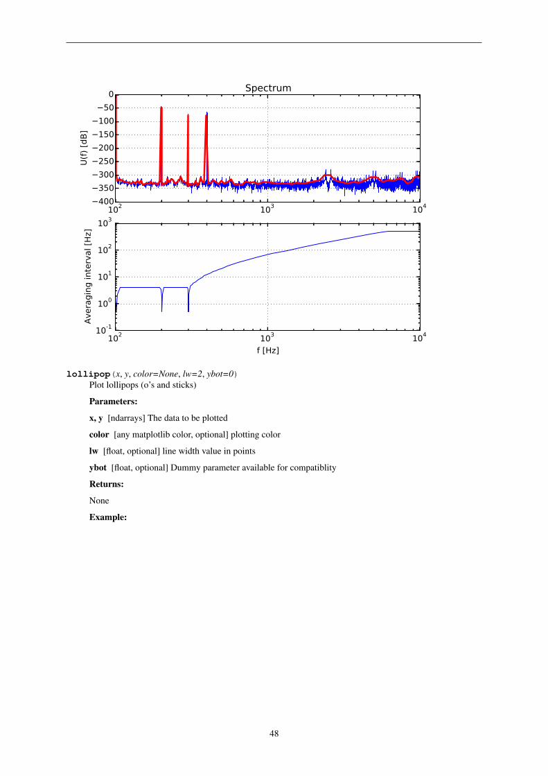
lollipop(x, y, color=None, lw=2, ybot=0)Plot lollipops (o’s and sticks)

Parameters:

x, y [ndarrays] The data to be plotted

color [any matplotlib color, optional] plotting color

lw [float, optional] line width value in points

ybot [float, optional] Dummy parameter available for compatiblity

Returns:

None

Example:

48

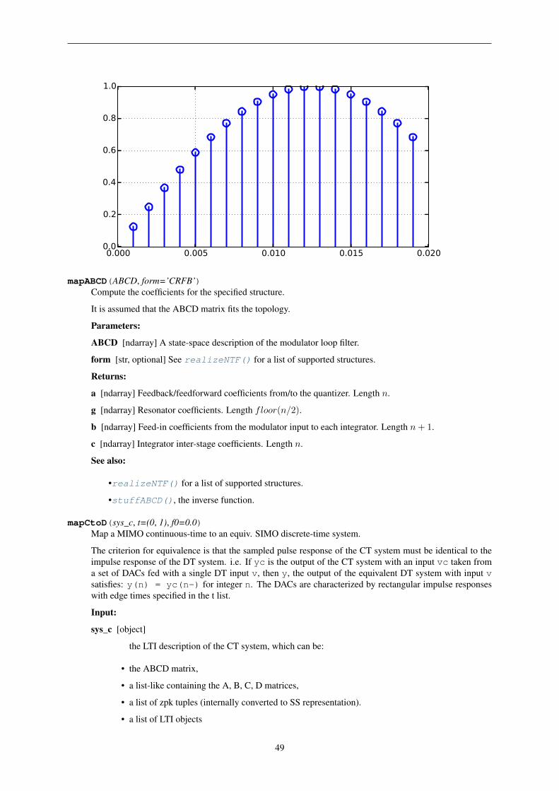
0.000 0.005 0.010 0.015 0.0200.0

0.2

0.4

0.6

0.8

1.0

mapABCD(ABCD, form=’CRFB’)Compute the coefficients for the specified structure.

It is assumed that the ABCD matrix fits the topology.

Parameters:

ABCD [ndarray] A state-space description of the modulator loop filter.

form [str, optional] See realizeNTF() for a list of supported structures.

Returns:

a [ndarray] Feedback/feedforward coefficients from/to the quantizer. Length 𝑛.

g [ndarray] Resonator coefficients. Length 𝑓𝑙𝑜𝑜𝑟(𝑛/2).

b [ndarray] Feed-in coefficients from the modulator input to each integrator. Length 𝑛+ 1.

c [ndarray] Integrator inter-stage coefficients. Length 𝑛.

See also:

•realizeNTF() for a list of supported structures.

•stuffABCD(), the inverse function.

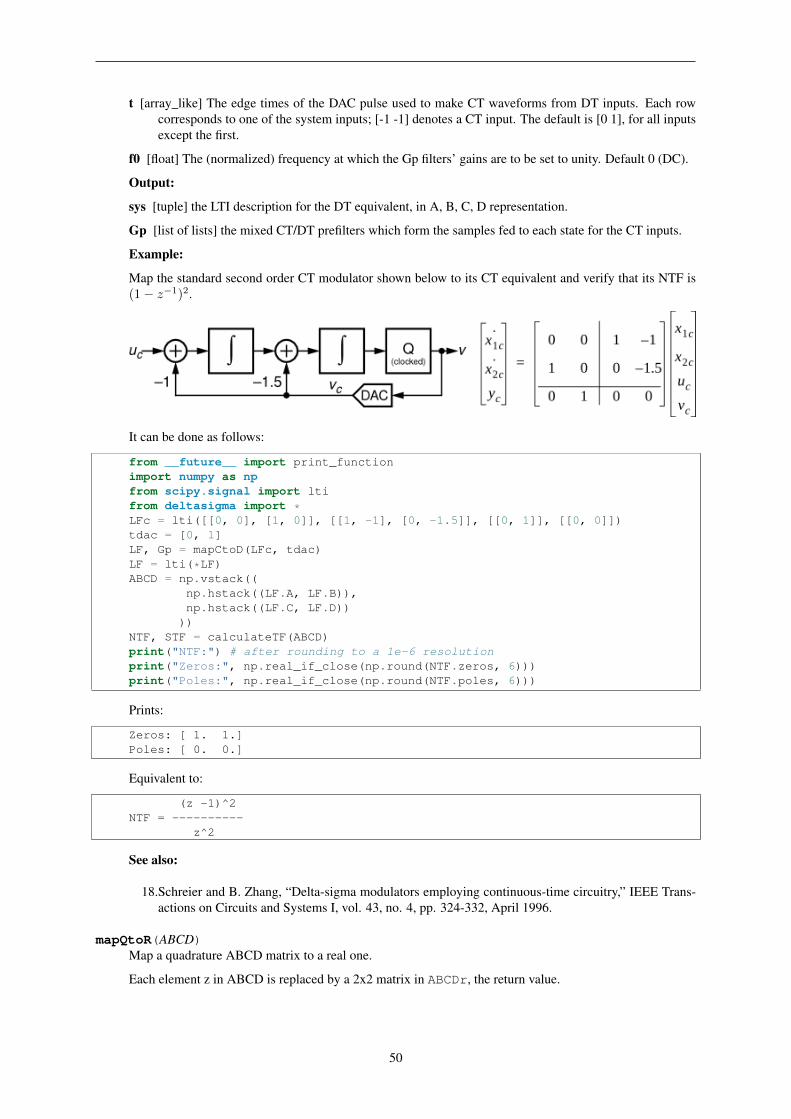
mapCtoD(sys_c, t=(0, 1), f0=0.0)Map a MIMO continuous-time to an equiv. SIMO discrete-time system.

The criterion for equivalence is that the sampled pulse response of the CT system must be identical to theimpulse response of the DT system. i.e. If yc is the output of the CT system with an input vc taken froma set of DACs fed with a single DT input v, then y, the output of the equivalent DT system with input vsatisfies: y(n) = yc(n-) for integer n. The DACs are characterized by rectangular impulse responseswith edge times specified in the t list.

Input:

sys_c [object]

the LTI description of the CT system, which can be:

• the ABCD matrix,

• a list-like containing the A, B, C, D matrices,

• a list of zpk tuples (internally converted to SS representation).

• a list of LTI objects

49

t [array_like] The edge times of the DAC pulse used to make CT waveforms from DT inputs. Each rowcorresponds to one of the system inputs; [-1 -1] denotes a CT input. The default is [0 1], for all inputsexcept the first.

f0 [float] The (normalized) frequency at which the Gp filters’ gains are to be set to unity. Default 0 (DC).

Output:

sys [tuple] the LTI description for the DT equivalent, in A, B, C, D representation.

Gp [list of lists] the mixed CT/DT prefilters which form the samples fed to each state for the CT inputs.

Example:

Map the standard second order CT modulator shown below to its CT equivalent and verify that its NTF is(1− 𝑧−1)2.

It can be done as follows:

from __future__ import print_functionimport numpy as npfrom scipy.signal import ltifrom deltasigma import *LFc = lti([[0, 0], [1, 0]], [[1, -1], [0, -1.5]], [[0, 1]], [[0, 0]])tdac = [0, 1]LF, Gp = mapCtoD(LFc, tdac)LF = lti(*LF)ABCD = np.vstack((

np.hstack((LF.A, LF.B)),np.hstack((LF.C, LF.D))

))NTF, STF = calculateTF(ABCD)print("NTF:") # after rounding to a 1e-6 resolutionprint("Zeros:", np.real_if_close(np.round(NTF.zeros, 6)))print("Poles:", np.real_if_close(np.round(NTF.poles, 6)))

Prints:

Zeros: [ 1. 1.]Poles: [ 0. 0.]

Equivalent to:

(z -1)^2NTF = ----------

z^2

See also:

18.Schreier and B. Zhang, “Delta-sigma modulators employing continuous-time circuitry,” IEEE Trans-actions on Circuits and Systems I, vol. 43, no. 4, pp. 324-332, April 1996.

mapQtoR(ABCD)Map a quadrature ABCD matrix to a real one.

Each element z in ABCD is replaced by a 2x2 matrix in ABCDr, the return value.

50

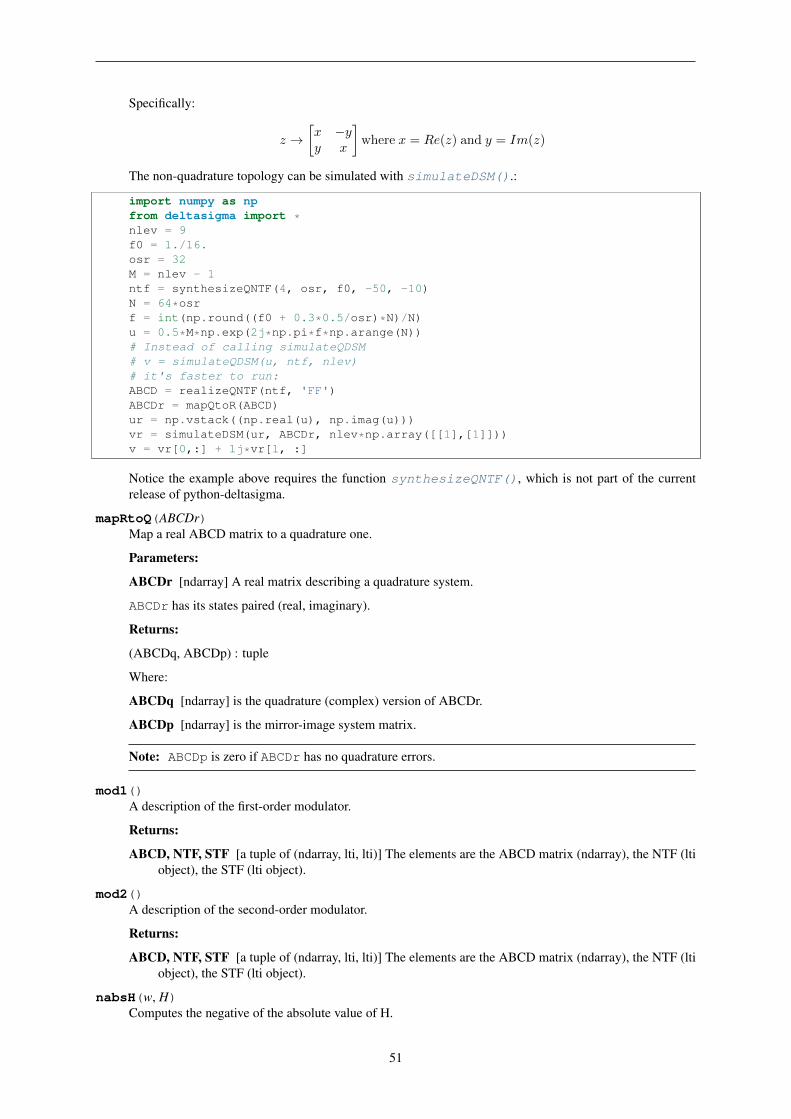
Specifically:

𝑧 →[𝑥 −𝑦𝑦 𝑥

]where 𝑥 = 𝑅𝑒(𝑧) and 𝑦 = 𝐼𝑚(𝑧)

The non-quadrature topology can be simulated with simulateDSM().:

import numpy as npfrom deltasigma import *nlev = 9f0 = 1./16.osr = 32M = nlev - 1ntf = synthesizeQNTF(4, osr, f0, -50, -10)N = 64*osrf = int(np.round((f0 + 0.3*0.5/osr)*N)/N)u = 0.5*M*np.exp(2j*np.pi*f*np.arange(N))# Instead of calling simulateQDSM# v = simulateQDSM(u, ntf, nlev)# it's faster to run:ABCD = realizeQNTF(ntf, 'FF')ABCDr = mapQtoR(ABCD)ur = np.vstack((np.real(u), np.imag(u)))vr = simulateDSM(ur, ABCDr, nlev*np.array([[1],[1]]))v = vr[0,:] + 1j*vr[1, :]

Notice the example above requires the function synthesizeQNTF(), which is not part of the currentrelease of python-deltasigma.

mapRtoQ(ABCDr)Map a real ABCD matrix to a quadrature one.

Parameters:

ABCDr [ndarray] A real matrix describing a quadrature system.

ABCDr has its states paired (real, imaginary).

Returns:

(ABCDq, ABCDp) : tuple

Where:

ABCDq [ndarray] is the quadrature (complex) version of ABCDr.

ABCDp [ndarray] is the mirror-image system matrix.

Note: ABCDp is zero if ABCDr has no quadrature errors.

mod1()A description of the first-order modulator.

Returns:

ABCD, NTF, STF [a tuple of (ndarray, lti, lti)] The elements are the ABCD matrix (ndarray), the NTF (ltiobject), the STF (lti object).

mod2()A description of the second-order modulator.

Returns:

ABCD, NTF, STF [a tuple of (ndarray, lti, lti)] The elements are the ABCD matrix (ndarray), the NTF (ltiobject), the STF (lti object).

nabsH(w, H)Computes the negative of the absolute value of H.

51

The computation is performed at the specified angular frequency w, on the unit circle.

This function is used by infnorm().

padb(x, n, val=0.0)Pad a matrix x on the bottom to length n with value val.

Parameters:

x [ndarray] The matrix to be padded.

n [int] The number of rows of the matrix after padding.

val [scalar, optional] The value to be used used for padding.

Note: A 1-d array, for example a.shape == (N,) is reshaped to be a 1 column array:a.reshape((N, 1))

The empty matrix is assumed to be have 1 empty column.

Returns:

xp [2-d ndarray] The padded matrix.

padl(x, n, val=0.0)Pad a matrix x on the left to length n with value val.

Parameters:

x [ndarray] The matrix to be padded.

n [int] The number of colums of the matrix after padding.

val [scalar, optional] The value to be used used for padding.

Note: A 1-d array, for example a.shape == (N,) is reshaped to be a 1 row array: a.reshape((1,N))

The empty matrix is assumed to be have 1 empty row.

Returns:

xp [2-d ndarray] The padded matrix.

padr(x, n, val=0.0)Pad a matrix x on the right to length n with value val.

Parameters:

x [ndarray] The matrix to be padded.

n [int] The number of colums of the matrix after padding.

val [scalar, optional] The value to be used used for padding.

Note: A 1-d array, for example a.shape == (N,) is reshaped to be a 1 row array: a.reshape((1,N))

The empty matrix is assumed to be have 1 empty row.

Returns:

xp [2-d ndarray] The padded matrix.

padt(x, n, val=0.0)Pad a matrix x on the top to length n with value val.

Parameters:

x [ndarray] The matrix to be padded.

52

n [int] The number of rows of the matrix after padding.

val [scalar, optional] The value to be used used for padding.

Note: A 1-d array, for example a.shape == (N,) is reshaped to be a 1 column array:a.reshape((N, 1))

The empty matrix is assumed to be have 1 empty column.

Returns:

xp [2-d ndarray] The padded matrix.

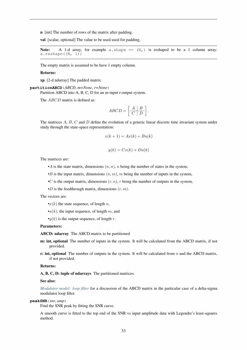
partitionABCD(ABCD, m=None, r=None)Partition ABCD into A, B, C, D for an m-input r-output system.

The 𝐴𝐵𝐶𝐷 matrix is defined as:

𝐴𝐵𝐶𝐷 =

[𝐴 𝐵𝐶 𝐷

].

The matrices 𝐴, 𝐵, 𝐶 and 𝐷 define the evolution of a generic linear discrete time invariant system understudy through the state-space representation:

𝑥(𝑘 + 1) = 𝐴𝑥(𝑘) +𝐵𝑢(𝑘)

𝑦(𝑘) = 𝐶𝑥(𝑘) +𝐷𝑢(𝑘)

The matrices are:

•𝐴 is the state matrix, dimensions (𝑛, 𝑛), 𝑛 being the number of states in the system,

•𝐵 is the input matrix, dimensions (𝑛,𝑚), 𝑚 being the number of inputs in the system,

•𝐶 is the output matrix, dimensions (𝑟, 𝑛), 𝑟 being the number of outputs in the system,

•𝐷 is the feedthrough matrix, dimensions (𝑟,𝑚).

The vectors are:

•𝑥(𝑘) the state sequence, of length 𝑛,

•𝑢(𝑘), the input sequence, of length 𝑚, and

•𝑦(𝑘) is the output sequence, of length 𝑟.

Parameters:

ABCD: ndarray The ABCD matrix to be partitioned

m: int, optional The number of inputs in the system. It will be calculated from the ABCD matrix, if notprovided.

r: int, optional The number of outputs in the system. It will be calculated from m and the ABCD matrix,if not provided.

Returns:

A, B, C, D: tuple of ndarrays The partitioned matrices.

See also:

Modulator model: loop filter for a discussion of the ABCD matrix in the particular case of a delta-sigmamodulator loop filter.

peakSNR(snr, amp)Find the SNR peak by fitting the SNR curve.

A smooth curve is fitted to the top end of the SNR vs input amplitude data with Legendre’s least-squaresmethod.

53

The curve fitted to the data is:

𝑦 = 𝑎𝑥+𝑏

𝑥− 𝑐

Parameters:

snr [1D ndarray or array-like] Signal to Noise Ratio array, expressed in decibels (dB).

amp [1D ndarray or array-like] Amplitude array, expressed in decibels (dB).

The two arrays snr and amp should have the same size.

Returns:

(peak_snr, peak_amp) [tuple] The peak SNR value and its corresponding amplitude, expressed in dB.

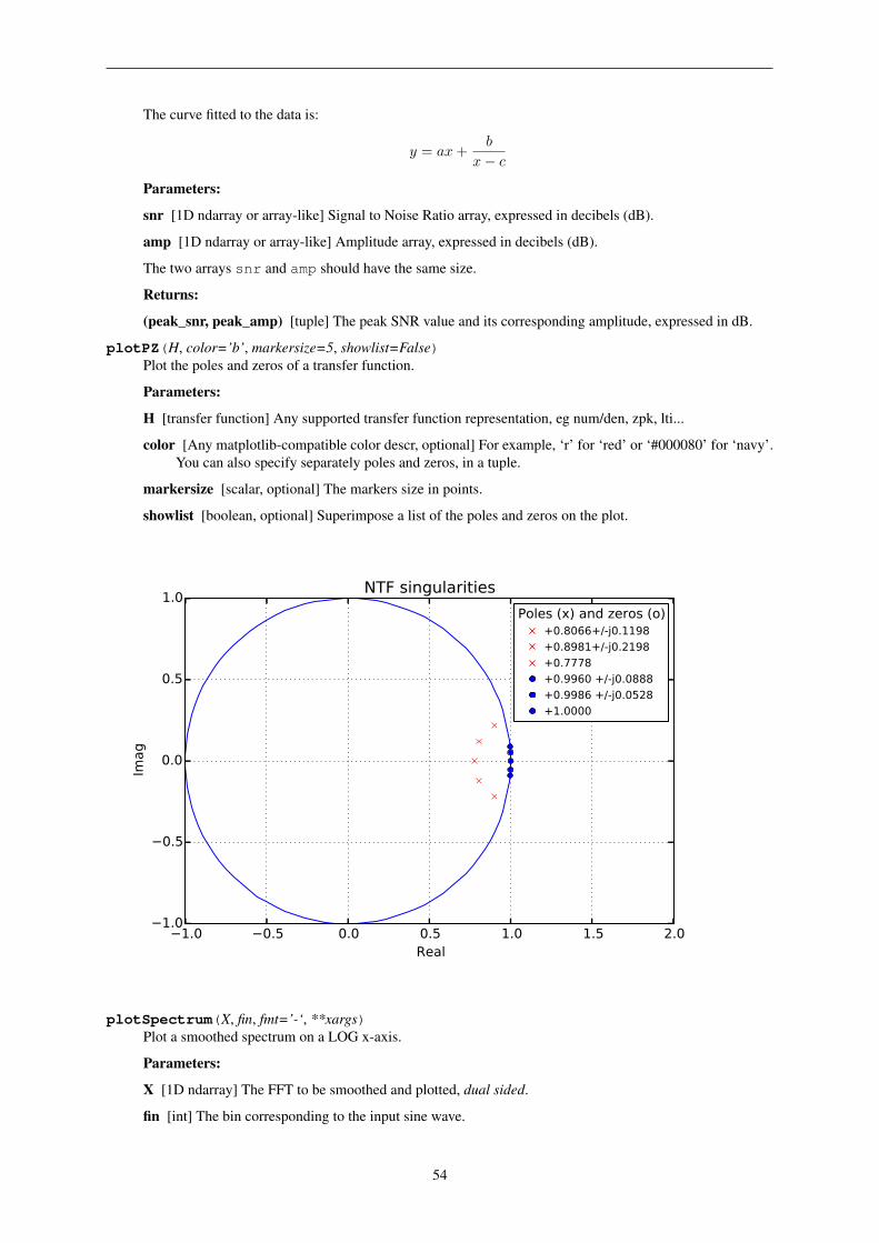
plotPZ(H, color=’b’, markersize=5, showlist=False)Plot the poles and zeros of a transfer function.

Parameters:

H [transfer function] Any supported transfer function representation, eg num/den, zpk, lti...

color [Any matplotlib-compatible color descr, optional] For example, ‘r’ for ‘red’ or ‘#000080’ for ‘navy’.You can also specify separately poles and zeros, in a tuple.

markersize [scalar, optional] The markers size in points.

showlist [boolean, optional] Superimpose a list of the poles and zeros on the plot.

1.0 0.5 0.0 0.5 1.0 1.5 2.0Real

1.0

0.5

0.0

0.5

1.0

Imag

NTF singularitiesPoles (x) and zeros (o)

+0.8066+/-j0.1198+0.8981+/-j0.2198+0.7778+0.9960 +/-j0.0888+0.9986 +/-j0.0528+1.0000

plotSpectrum(X, fin, fmt=’-‘, **xargs)Plot a smoothed spectrum on a LOG x-axis.

Parameters:

X [1D ndarray] The FFT to be smoothed and plotted, dual sided.

fin [int] The bin corresponding to the input sine wave.

54

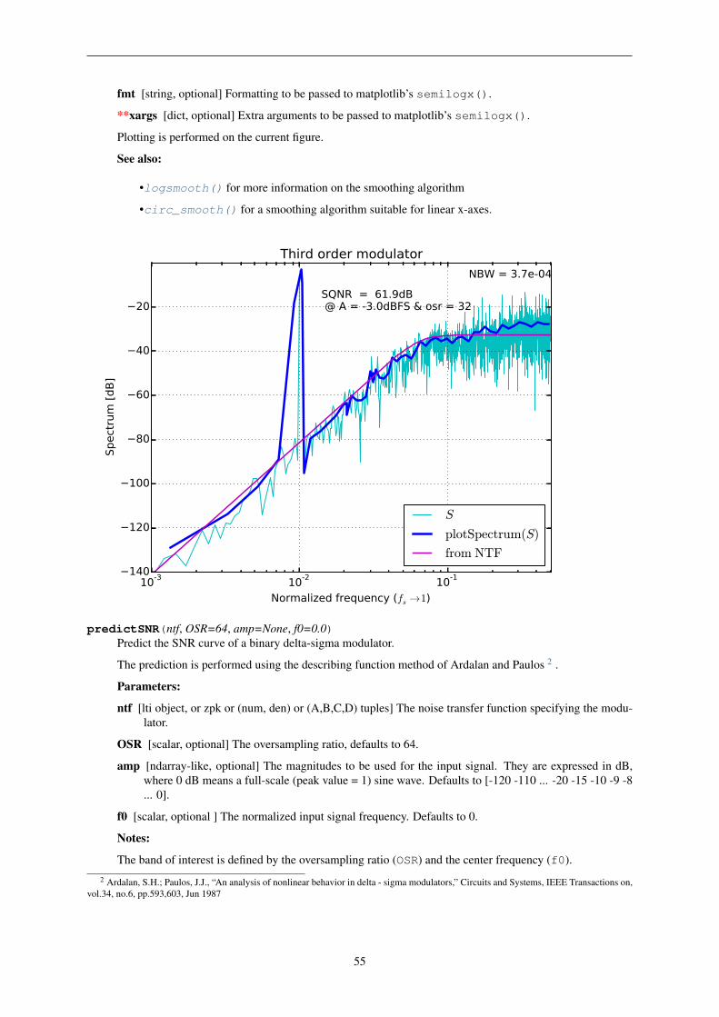
fmt [string, optional] Formatting to be passed to matplotlib’s semilogx().

**xargs [dict, optional] Extra arguments to be passed to matplotlib’s semilogx().

Plotting is performed on the current figure.

See also:

•logsmooth() for more information on the smoothing algorithm

•circ_smooth() for a smoothing algorithm suitable for linear x-axes.

10-3 10-2 10-1

Normalized frequency (fs →1)

140

120

100

80

60

40

20

Spec

trum

[dB]

SQNR = 61.9dB @ A = -3.0dBFS & osr = 32

NBW = 3.7e-04 Third order modulator

S

plotSpectrum(S)

from NTF

predictSNR(ntf, OSR=64, amp=None, f0=0.0)Predict the SNR curve of a binary delta-sigma modulator.

The prediction is performed using the describing function method of Ardalan and Paulos 2 .

Parameters:

ntf [lti object, or zpk or (num, den) or (A,B,C,D) tuples] The noise transfer function specifying the modu-lator.

OSR [scalar, optional] The oversampling ratio, defaults to 64.

amp [ndarray-like, optional] The magnitudes to be used for the input signal. They are expressed in dB,where 0 dB means a full-scale (peak value = 1) sine wave. Defaults to [-120 -110 ... -20 -15 -10 -9 -8... 0].

f0 [scalar, optional ] The normalized input signal frequency. Defaults to 0.

Notes:

The band of interest is defined by the oversampling ratio (OSR) and the center frequency (f0).

2 Ardalan, S.H.; Paulos, J.J., “An analysis of nonlinear behavior in delta - sigma modulators,” Circuits and Systems, IEEE Transactions on,vol.34, no.6, pp.593,603, Jun 1987

55

The algorithm assumes that the amp vector is sorted in increasing order; once instability is detected, theremaining SNR values are set to -Inf.

Future versions may accommodate STFs.

Returns:

snr [ndarray] A vector of SNR values, in dB.

amp [ndarray] A vector of amplitudes, in dB.

k0 [ndarray] The quantizer signal gain.

k1: ndarray The quantizer noise gain.

sigma_e2 [scalar] The power of the quantizer noise (not in dB).

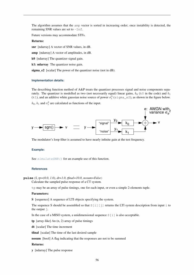
Implementation details:

The describing function method of A&P treats the quantizer processes signal and noise components sepa-rately. The quantizer is modelled as two (not necessarily equal) linear gains, 𝑘0 (k0 in the code) and 𝑘1(k1), and an additive white gaussian noise source of power 𝜎2

𝑒 (sigma_e2), as shown in the figure below.

𝑘0, 𝑘1 and 𝜎2𝑒 are calculated as functions of the input.

The modulator’s loop filter is assumed to have nearly infinite gain at the test frequency.

Example:

See simulateSNR() for an example use of this function.

References

pulse(S, tp=(0.0, 1.0), dt=1.0, tfinal=10.0, nosum=False)Calculate the sampled pulse response of a CT system.

tp may be an array of pulse timings, one for each input, or even a simple 2-elements tuple.

Parameters:

S [sequence] A sequence of LTI objects specifying the system.

The sequence S should be assembled so that S[i][j] returns the LTI system description from input i tothe output j.

In the case of a MISO system, a unidimensional sequence S[i] is also acceptable.

tp [array-like] An (n, 2) array of pulse timings

dt [scalar] The time increment

tfinal [scalar] The time of the last desired sample

nosum [bool] A flag indicating that the responses are not to be summed

Returns:

y [ndarray] The pulse response

56

realizeNTF(ntf, form=’CRFB’, stf=None)Convert an NTF into coefficients for the desired structure.

Parameters:

ntf [a zpk transfer function] The modulator noise transfer function (NTF)

form [string] A structure identifier.

Supported structures are:

•“CRFB”: Cascade of resonators, feedback form.

•“CRFF”: Cascade of resonators, feedforward form.

•“CIFB”: Cascade of integrators, feedback form.

•“CIFF”: Cascade of integrators, feedforward form.

•“CRFBD”: CRFB with delaying quantizer.

•“CRFFD”: CRFF with delaying quantizer.

•“PFF”: Parallel feed-forward.

•“Stratos”: A CIFF-like structure with non-delaying resonator feedbacks, contributed to the MATLABDelta Sigma toolbox in 2007 by Jeff Gealow.

See the accompanying documentation (Topologies diagrams) for block diagrams of each structure.

stf [a zpk transfer function, optional] the Signal Transfer Function

Returns:

a, g, b, c [tuple of ndarrays] the coefficients for the desired structure

Example:

Determine the coefficients for a 5th-order modulator with the cascade-of-resonators structure, feedback(CRFB) form.:

from deltasigma import synthesizeNTF, realizeNTFH = synthesizeNTF(5, 32, 1)a, g, b, c = realizeNTF(H,'CRFB')

Returns the values:

a: 0.0007, 0.0084, 0.055, 0.2443, 0.5579g: 0.0028, 0.0079b: 0.0007, 0.0084, 0.055, 0.2443, 0.5579, 1.0c: 1.0, 1.0, 1.0, 1.0, 1.0

realizeNTF_ct(ntf, form=’FB’, tdac=(0, 1), ordering=None, bp=None, ABCDc=None,method=’LOOP’)

Realize an NTF with a continuous-time loop filter.

Parameters:

ntf [object] A noise transfer function (NTF).

form [str, optional] A string specifying the topology of the loop filter.

• ‘FB’: Feedback form,

• ‘FF’: Feedforward form

For the FB structure, the elements of Bc are calculated so that the sampled pulse response matches theL1 impulse response. For the FF structure, Cc is calculated.

tdac [sequence, optional] The timing for the feedback DAC(s). If tdac[0] >= 1, direct feedback termsare added to the quantizer.

57

Multiple timings (one or more per integrator) for the FB topology can be specified by making tdac alist of lists, e.g. tdac = [[1, 2], [1, 2], [[0.5, 1], [1, 1.5]], []]

In this example, the first two integrators have DACs with [1, 2] timing, the third has a pair of DACs,one with [0.5, 1] timing and the other with [1, 1.5] timing, and there is no direct feedbackDAC to the quantizer.

ordering [sequence, optional] A vector specifying which NTF zero-pair to use in each resonator Default isfor the zero-pairs to be used in the order specified in the NTF.

bp [sequence, optional] A vector specifying which resonator sections are bandpass. The default(zeros(...)) is for all sections to be lowpass.

ABCDc [ndarray, optional] The loop filter structure, in state-space form. If this argument is omitted,ABCDc is constructed according to “form.”

method [str, optional] The default fitting method is ’LOOP’, which means that the DT and CT loop re-sponses will be matched. Alternatively, it is possible to set the method to ’NTF’, which will result inthe NTF responses to be matched. See Discrete time to continuous time mapping for a more in-depthdiscussion.

Returns:

ABCDc [ndarray] A state-space description of the CT loop filter

tdac2 [ndarray] A matrix with the DAC timings, including ones that were automatically added.

Example:

Realize the NTF (1− 𝑧−1)2 with a CT system (cf with the example at mapCtoD()).:

from deltasigma import *ntf = ([1, 1], [0, 0], 1)ABCDc, tdac2 = realizeNTF_ct(ntf, 'FB')

Returns:

ABCDc:

[[ 0. 0. 1. -1. ][ 1. 0. 0. -1.49999999][ 0. 1. 0. 0. ]]

tdac2:

[[-1. -1.][ 0. 1.]]

realizeQNTF(ntf, form=’FB’, rot=False, bn=0.0)Convert a quadrature NTF into an ABCD matrix

The basic idea is to equate the value of the loop filter at a set of points in the z-plane to the values of𝐿1 = 1− 1/𝐻 at those points.

The order of the zeros is used when mapping the NTF onto the chosen topology.

Supported structures are:

•‘FB’: Feedback

•‘PFB’: Parallel feedback

•‘FF’: Feedforward (bn is the coefficient of the aux DAC)

•‘PFF’: Parallel feedforward

Not currently supported - feel free to send in a patch:

•‘FBD’: FB with delaying quantizer

•‘FFD’: FF with delaying quantizer

58

Parameters:

ntf [lti object or supported description] The NTF to be converted.

form [str, optional] The form to be used. See above for the currently supported topologies. Defaults to’FB’.

rot [bool, optional] Set rot to True to rotate the states to make as many coefficients as possible real.

bn [float, optional] Coefficient of the auxiliary DAC, to be specified for a ‘FF’ form. Defaults to 0.0.

Returns:

ABCD [ndarray] ABCD realization of the requested type.

rms(x, no_dc=False)Calculate the RMS value of x.

The Root Mean Square value of an array 𝑥 of length 𝑛 is defined as:

𝑥𝑅𝑀𝑆 =

√1

𝑛(𝑥2

1 + 𝑥22 + ...+ 𝑥2

𝑛)

Parameters:

x [(N,) ndarray] The input vector

no_dc [boolean, optional] If set to True, the DC value gets subtracted from x first and the RMS is com-puted on the result.

Returns:

xrms [scalar] as defined above

rmsGain(H, f1, f2, N=100)Compute the root mean-square gain of a discrete-time TF.

The computation is carried out over the frequency band (f1, f2), employing N discretization steps.

Parameters:

H [object] The discrete-time transfer function. See evalTF() for the supported types.

f1 [scalar] The start value in Hertz of the frequency band over which the gain is evaluated.

f2 [scalar] The end value (inclusive) in Hertz of the aforementioned frequency band.

N [integer, optional] The number of discretization points to be taken over specified interval.

Returns:

Grms [scalar] The root mean-square gain

scaleABCD(ABCD, nlev=2, f=0, xlim=1, ymax=None, umax=None, N_sim=100000.0, N0=10)Scale the loop filter of a general delta-sigma modulator for dynamic range.

The ABCD matrix is scaled so that the state maxima are less than the specified limits (xlim). As a sideeffect, the maximum stable input is determined in the process.

Parameters:

ABCD [ndarray] The state-space description of the loop filter, real or imaginary (quadrature).

nlev [int, optional] The number of levels in the quantizer.

f [scalar] The normalized frequency of the test sinusoid.

xlim [scalar or ndarray] A vector or scalar specifying the limit for each state variable.

ymax [scalar, optional] The stability threshold. Inputs that yield quantizer inputs above ymax are consid-ered to be beyond the stable range of the modulator. If not provided, it will be set to 𝑛𝑙𝑒𝑣 + 5

umax [scalar, optional] The maximum allowable input amplitude. umax is calculated if it is not supplied.

59

Returns:

ABCDs [ndarray] The state-space description of the scaled loop filter.

umax [scalar] The maximum stable input amplitude. Input sinusoids with amplitudes below this valueshould not cause the modulator states to exceed their specified limits.

S [ndarray] The diagonal scaling matrix S.

S is defined such that:

ABCDs = [[S*A*Sinv, S*B], [C*Sinv, D]]xs = S*x

Where the multiplications are matrix multiplications.

simulateDSM(u, arg2, nlev=2, x0=0.0)Simulate a Delta Sigma modulator

Compute the output of a general delta-sigma modulator with input u, a structure described by ABCD, aninitial state x0 (default zero) and a quantizer with a number of levels specified by nlev.

Syntax:

•[v, xn, xmax, y] = simulateDSM(u, ABCD, nlev=2, x0=0)

•[v, xn, xmax, y] = simulateDSM(u, ntf, nlev=2, x0=0)

Parameters:

u [ndarray or sequence] The input vector to be used in the simulation. Multiple inputs are implied by thenumber of rows in u.

arg2 [2D ndarray or a supported LTI description] The second argument may be either the ABCD matrixdescribing the modulator or its NTF. In the latter case, the NTF is converted to a ZPK description andthe structure that is simulated is the block-diagonal structure used by scipy’s zpk2ss(). The STF isassumed to be 1.

nlev [int or sequence or ndarray] Number of levels in the quantizers. Set nlev to a scalar for a signlequantizer modulator. Multiple quantizers are implied by making nlev an array.

x0 [float or sequence or ndarray] The initial status of the modulator. If x0 is set to float, its value will beused for all the states. If it is set to a sequence of floats, each of its values will be assigned to a statevariable.

Returns:

v [ndarray] The quantizer output.

xn [ndarray] The modulator states.

xmax [nedarray] The maximum value that each state reached during simulation.

y [ndarray] The quantizer input (ie the modulator output).

Notes:

Three implementations of this function are (potentially) available to the user, in order of ascending executionspeed:

•A CPython implementation, always available.

•A Cython-based implementation requiring the BLAS headers and a compatible compiler.

•A Cython-based implementation accessing the BLAS library pre-compiled through scipy, requiringonly a compatible compiler.

The difference in execution time from the first implementation – dynamically interpreted – to the latter two– statically compiled automatically before execution – is a factor 20.

The fastest available implementation is automatically selected.

60

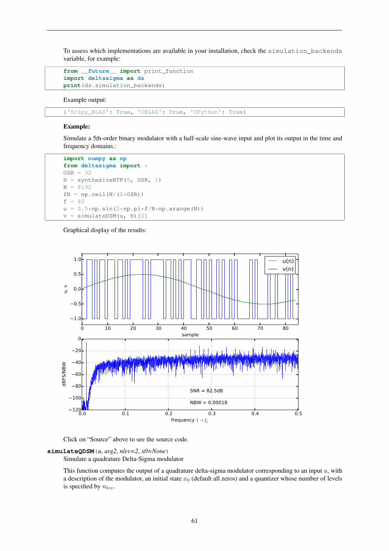
To assess which implementations are available in your installation, check the simulation_backendsvariable, for example:

from __future__ import print_functionimport deltasigma as dsprint(ds.simulation_backends)

Example output:

{'Scipy_BLAS': True, 'CBLAS': True, 'CPython': True}

Example:

Simulate a 5th-order binary modulator with a half-scale sine-wave input and plot its output in the time andfrequency domains.:

import numpy as npfrom deltasigma import *OSR = 32H = synthesizeNTF(5, OSR, 1)N = 8192fB = np.ceil(N/(2*OSR))f = 85u = 0.5*np.sin(2*np.pi*f/N*np.arange(N))v = simulateDSM(u, H)[0]

Graphical display of the results:

0 10 20 30 40 50 60 70 80sample

1.0

0.5

0.0

0.5

1.0

u, v

u(n)v(n)

0.0 0.1 0.2 0.3 0.4 0.5frequency 1→fs

120

100

80

60

40

20

0

dBFS

/NBW

SNR = 82.5dB

NBW = 0.00018

Click on “Source” above to see the source code.

simulateQDSM(u, arg2, nlev=2, x0=None)Simulate a quadrature Delta-Sigma modulator

This function computes the output of a quadrature delta-sigma modulator corresponding to an input 𝑢, witha description of the modulator, an initial state 𝑥0 (default all zeros) and a quantizer whose number of levelsis specified by 𝑛𝑙𝑒𝑣.

61

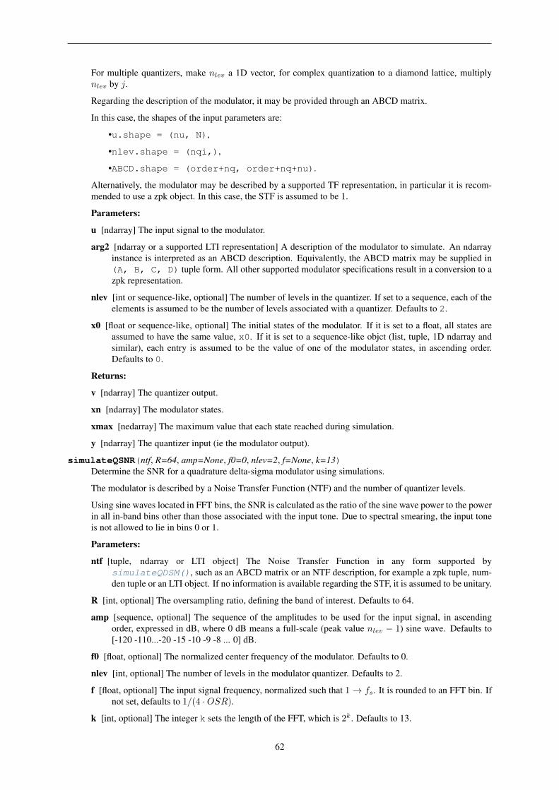
For multiple quantizers, make 𝑛𝑙𝑒𝑣 a 1D vector, for complex quantization to a diamond lattice, multiply𝑛𝑙𝑒𝑣 by 𝑗.

Regarding the description of the modulator, it may be provided through an ABCD matrix.

In this case, the shapes of the input parameters are:

•u.shape = (nu, N),

•nlev.shape = (nqi,),

•ABCD.shape = (order+nq, order+nq+nu).

Alternatively, the modulator may be described by a supported TF representation, in particular it is recom-mended to use a zpk object. In this case, the STF is assumed to be 1.

Parameters:

u [ndarray] The input signal to the modulator.

arg2 [ndarray or a supported LTI representation] A description of the modulator to simulate. An ndarrayinstance is interpreted as an ABCD description. Equivalently, the ABCD matrix may be supplied in(A, B, C, D) tuple form. All other supported modulator specifications result in a conversion to azpk representation.

nlev [int or sequence-like, optional] The number of levels in the quantizer. If set to a sequence, each of theelements is assumed to be the number of levels associated with a quantizer. Defaults to 2.

x0 [float or sequence-like, optional] The initial states of the modulator. If it is set to a float, all states areassumed to have the same value, x0. If it is set to a sequence-like objct (list, tuple, 1D ndarray andsimilar), each entry is assumed to be the value of one of the modulator states, in ascending order.Defaults to 0.

Returns:

v [ndarray] The quantizer output.

xn [ndarray] The modulator states.

xmax [nedarray] The maximum value that each state reached during simulation.

y [ndarray] The quantizer input (ie the modulator output).

simulateQSNR(ntf, R=64, amp=None, f0=0, nlev=2, f=None, k=13)Determine the SNR for a quadrature delta-sigma modulator using simulations.

The modulator is described by a Noise Transfer Function (NTF) and the number of quantizer levels.

Using sine waves located in FFT bins, the SNR is calculated as the ratio of the sine wave power to the powerin all in-band bins other than those associated with the input tone. Due to spectral smearing, the input toneis not allowed to lie in bins 0 or 1.

Parameters:

ntf [tuple, ndarray or LTI object] The Noise Transfer Function in any form supported bysimulateQDSM(), such as an ABCD matrix or an NTF description, for example a zpk tuple, num-den tuple or an LTI object. If no information is available regarding the STF, it is assumed to be unitary.

R [int, optional] The oversampling ratio, defining the band of interest. Defaults to 64.

amp [sequence, optional] The sequence of the amplitudes to be used for the input signal, in ascendingorder, expressed in dB, where 0 dB means a full-scale (peak value 𝑛𝑙𝑒𝑣 − 1) sine wave. Defaults to[-120 -110...-20 -15 -10 -9 -8 ... 0] dB.

f0 [float, optional] The normalized center frequency of the modulator. Defaults to 0.

nlev [int, optional] The number of levels in the modulator quantizer. Defaults to 2.

f [float, optional] The input signal frequency, normalized such that 1 → 𝑓𝑠. It is rounded to an FFT bin. Ifnot set, defaults to 1/(4 ·𝑂𝑆𝑅).

k [int, optional] The integer k sets the length of the FFT, which is 2𝑘. Defaults to 13.

62

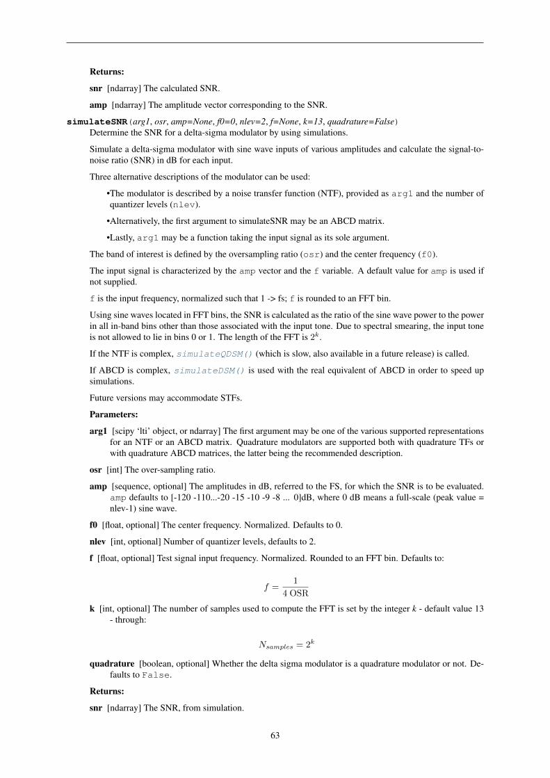
Returns:

snr [ndarray] The calculated SNR.

amp [ndarray] The amplitude vector corresponding to the SNR.

simulateSNR(arg1, osr, amp=None, f0=0, nlev=2, f=None, k=13, quadrature=False)Determine the SNR for a delta-sigma modulator by using simulations.

Simulate a delta-sigma modulator with sine wave inputs of various amplitudes and calculate the signal-to-noise ratio (SNR) in dB for each input.

Three alternative descriptions of the modulator can be used:

•The modulator is described by a noise transfer function (NTF), provided as arg1 and the number ofquantizer levels (nlev).

•Alternatively, the first argument to simulateSNR may be an ABCD matrix.

•Lastly, arg1 may be a function taking the input signal as its sole argument.

The band of interest is defined by the oversampling ratio (osr) and the center frequency (f0).

The input signal is characterized by the amp vector and the f variable. A default value for amp is used ifnot supplied.

f is the input frequency, normalized such that 1 -> fs; f is rounded to an FFT bin.

Using sine waves located in FFT bins, the SNR is calculated as the ratio of the sine wave power to the powerin all in-band bins other than those associated with the input tone. Due to spectral smearing, the input toneis not allowed to lie in bins 0 or 1. The length of the FFT is 2𝑘.

If the NTF is complex, simulateQDSM() (which is slow, also available in a future release) is called.

If ABCD is complex, simulateDSM() is used with the real equivalent of ABCD in order to speed upsimulations.

Future versions may accommodate STFs.

Parameters:

arg1 [scipy ‘lti’ object, or ndarray] The first argument may be one of the various supported representationsfor an NTF or an ABCD matrix. Quadrature modulators are supported both with quadrature TFs orwith quadrature ABCD matrices, the latter being the recommended description.

osr [int] The over-sampling ratio.

amp [sequence, optional] The amplitudes in dB, referred to the FS, for which the SNR is to be evaluated.amp defaults to [-120 -110...-20 -15 -10 -9 -8 ... 0]dB, where 0 dB means a full-scale (peak value =nlev-1) sine wave.

f0 [float, optional] The center frequency. Normalized. Defaults to 0.

nlev [int, optional] Number of quantizer levels, defaults to 2.

f [float, optional] Test signal input frequency. Normalized. Rounded to an FFT bin. Defaults to:

𝑓 =1

4 OSR

k [int, optional] The number of samples used to compute the FFT is set by the integer k - default value 13- through:

𝑁𝑠𝑎𝑚𝑝𝑙𝑒𝑠 = 2𝑘

quadrature [boolean, optional] Whether the delta sigma modulator is a quadrature modulator or not. De-faults to False.

Returns:

snr [ndarray] The SNR, from simulation.

63

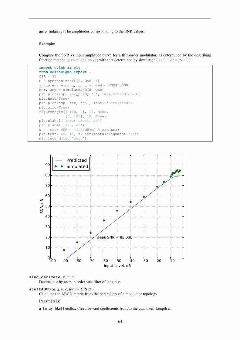
amp [ndarray] The amplitudes corresponding to the SNR values.

Example:

Compare the SNR vs input amplitude curve for a fifth-order modulator, as determined by the describingfunction method (predictSNR()) with that determined by simulation (simulateSNR()).:

import pylab as pltfrom deltasigma import *OSR = 32H = synthesizeNTF(5, OSR, 1)snr_pred, amp, _, _, _ = predictSNR(H,OSR)snr, amp = simulateSNR(H, OSR)plt.plot(amp, snr_pred, 'b', label='Predicted')plt.hold(True)plt.plot(amp, snr, 'go', label='Simulated')plt.grid(True)figureMagic([-100, 0], 10, None,

[0, 100], 10, None)plt.xlabel('Input Level, dB')plt.ylabel('SNR, dB')s = 'peak SNR = %4.1fdB\n' % max(snr)plt.text(-65, 15, s, horizontalalignment='left')plt.legend(loc='best')

100 90 80 70 60 50 40 30 20 10Input Level, dB

0

10

20

30

40

50

60

70

80

90

SNR,

dB

peak SNR = 85.0dB

PredictedSimulated

sinc_decimate(x, m, r)Decimate x by an m-th order sinc filter of length r.

stuffABCD(a, g, b, c, form=’CRFB’)Calculate the ABCD matrix from the parameters of a modulator topology.

Parameters:

a [array_like] Feedback/feedforward coefficients from/to the quantizer. Length 𝑛.

64

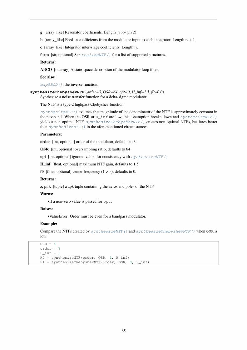
g [array_like] Resonator coefficients. Length 𝑓𝑙𝑜𝑜𝑟(𝑛/2).

b [array_like] Feed-in coefficients from the modulator input to each integrator. Length 𝑛+ 1.

c [array_like] Integrator inter-stage coefficients. Length 𝑛.

form [str, optional] See realizeNTF() for a list of supported structures.

Returns:

ABCD [ndarray] A state-space description of the modulator loop filter.

See also:

mapABCD(), the inverse function.

synthesizeChebyshevNTF(order=3, OSR=64, opt=0, H_inf=1.5, f0=0.0)Synthesize a noise transfer function for a delta-sigma modulator.

The NTF is a type-2 highpass Chebyshev function.

synthesizeNTF() assumes that magnitude of the denominator of the NTF is approximately constant inthe passband. When the OSR or H_inf are low, this assumption breaks down and synthesizeNTF()yields a non-optimal NTF. synthesizeChebyshevNTF() creates non-optimal NTFs, but fares betterthan synthesizeNTF() in the aforementioned circumstances.

Parameters:

order [int, optional] order of the modulator, defaults to 3

OSR [int, optional] oversampling ratio, defaults to 64

opt [int, optional] ignored value, for consistency with synthesizeNTF()

H_inf [float, optional] maximum NTF gain, defaults to 1.5

f0 [float, optional] center frequency (1->fs), defaults to 0.

Returns:

z, p, k [tuple] a zpk tuple containing the zeros and poles of the NTF.

Warns:

•If a non-zero value is passed for opt.

Raises:

•ValueError: Order must be even for a bandpass modulator.

Example:

Compare the NTFs created by synthesizeNTF() and synthesizeChebyshevNTF() when OSR islow:

OSR = 4order = 8H_inf = 3H0 = synthesizeNTF(order, OSR, 1, H_inf)H1 = synthesizeChebyshevNTF(order, OSR, 0, H_inf)

65

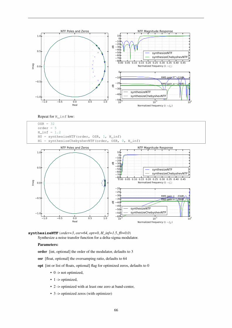
1.0 0.5 0.0 0.5 1.0Real

1.0

0.5

0.0

0.5

1.0Im

agNTF Poles and Zeros

0.00 0.05 0.10 0.15 0.20 0.25 0.30 0.35 0.40 0.45Normalized frequency (1→fs )

80706050403020100

10

dB

NTF Magnitude Response

synthesizeNTFsynthesizeChebyshevNTF

10-2 10-1 100

Normalized frequency (1→fB )

50

40

30

20

10

0

dB

RMS gain = -12dB

RMS gain = -24dB

synthesizeNTFsynthesizeChebyshevNTF

Repeat for H_inf low:

OSR = 32order = 5H_inf = 1.2H0 = synthesizeNTF(order, OSR, 1, H_inf)H1 = synthesizeChebyshevNTF(order, OSR, 0, H_inf)

1.0 0.5 0.0 0.5 1.0Real

1.0

0.5

0.0

0.5

1.0

Imag

NTF Poles and Zeros

0.00 0.05 0.10 0.15 0.20 0.25 0.30 0.35 0.40 0.45Normalized frequency (1→fs )

80706050403020100

10

dB

NTF Magnitude Response

synthesizeNTFsynthesizeChebyshevNTF

10-2 10-1 100

Normalized frequency (1→fB )

605550454035302520

dB

RMS gain = -33dBRMS gain = -38dB

synthesizeNTFsynthesizeChebyshevNTF

synthesizeNTF(order=3, osr=64, opt=0, H_inf=1.5, f0=0.0)Synthesize a noise transfer function for a delta-sigma modulator.

Parameters:

order [int, optional] the order of the modulator, defaults to 3

osr [float, optional] the oversamping ratio, defaults to 64

opt [int or list of floats, optional] flag for optimized zeros, defaults to 0

• 0 -> not optimized,

• 1 -> optimized,

• 2 -> optimized with at least one zero at band-center,

• 3 -> optimized zeros (with optimizer)

66

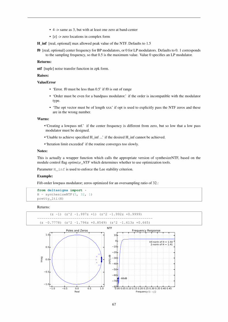
• 4 -> same as 3, but with at least one zero at band-center

• [z] -> zero locations in complex form

H_inf [real, optional] max allowed peak value of the NTF. Defaults to 1.5

f0 [real, optional] center frequency for BP modulators, or 0 for LP modulators. Defaults to 0. 1 correspondsto the sampling frequency, so that 0.5 is the maximum value. Value 0 specifies an LP modulator.

Returns:

ntf [tuple] noise transfer function in zpk form.

Raises:

ValueError

• ‘Error. f0 must be less than 0.5’ if f0 is out of range

• ‘Order must be even for a bandpass modulator.’ if the order is incompatible with the modulatortype.

• ‘The opt vector must be of length xxx’ if opt is used to explicitly pass the NTF zeros and theseare in the wrong number.

Warns:

•‘Creating a lowpass ntf.’ if the center frequency is different from zero, but so low that a low passmodulator must be designed.

•‘Unable to achieve specified H_inf ...’ if the desired H_inf cannot be achieved.

•‘Iteration limit exceeded’ if the routine converges too slowly.

Notes:

This is actually a wrapper function which calls the appropriate version of synthesizeNTF, based on themodule control flag optimize_NTF which determines whether to use optimization tools.

Parameter H_inf is used to enforce the Lee stability criterion.

Example:

Fift-order lowpass modulator; zeros optimized for an oversampling ratio of 32.:

from deltasigma import *H = synthesizeNTF(5, 32, 1)pretty_lti(H)

Returns:

(z -1) (z^2 -1.997z +1) (z^2 -1.992z +0.9999)--------------------------------------------------------(z -0.7778) (z^2 -1.796z +0.8549) (z^2 -1.613z +0.665)

1.0 0.5 0.0 0.5 1.0Real

1.0

0.5

0.0

0.5

1.0

Imag

Poles and Zeros

0.00 0.05 0.10 0.15 0.20 0.25 0.30 0.35 0.40 0.45Frequency (1→fs)

80

70

60

50

40

30

20

10

0

10

|H(f)

| dB

-66dB

Inf-norm of H = 1.50 2-norm of H = 1.41

Frequency ResponseNTF

67

See also:

clans() [Closed-Loop Analysis of Noise-Shaper.] An alternative method for selecting NTFs based onthe 1-norm of the impulse response of the NTF

synthesizeChebyshevNTF() [Select a type-2 highpass Chebyshev NTF.] This function does a betterjob than synthesizeNTF if osr or H_inf is low.

synthesizeQNTF(order=4, OSR=64, f0=0.0, NG=-60, ING=-20, n_im=None)Synthesize a noise transfer function for a quadrature modulator.

Parameters:

order [int, optional] The order of the modulator. Defaults to 4.

OSR [int, optional] The oversampling ratio. Defaults to 64.

f0 [float, optional] The center frequency, normalized such that 1 → 𝑓𝑠. Defaults to 0, ie to a low-passmodultor.

NG [float, optional] The in-band noise gain, expressed in dB. Defaults to -60.

ING [float, optional] The image-band noise gain, in dB. Defaults to -20.

n_im [int, optional] The number of in-band image zeros, defaults to floor(order/3).

Returns:

ntf [(z, p, k) tuple] ntf is a zpk tuple containing the zeros, poles and the gain of the synthesized NTF.

Note: From the Matlab Delta-Sigma Toobox: ALPHA VERSION: This function uses an experimentalad-hoc method that is neither optimal nor robust.

Example:

Fourth order quadrature modulator:

from deltasigma import *order = 4osr = 32NG = -50ING = -10f0 = 1 / 16ntf0 = synthesizeQNTF(order, osr, f0, NG, ING)pretty_lti(ntf0)

Returns:

(z - 0.888 - 0.4598j) (z - 0.9239 + 0.3827j) (z - 0.9239 - 0.3827j) (z - 0.953 - 0.3028j)---------------------------------------------------------------------------------------------(z - 0.5739 - 0.5699j) (z - 0.5913 - 0.2449j) (z - 0.6731 + 0.2788j) (z - 0.8088 - 0.0028j)

68

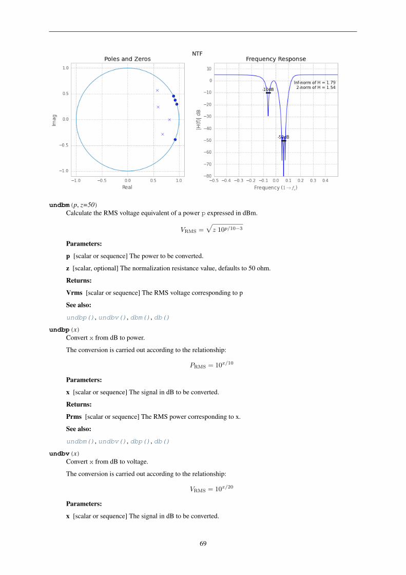
undbm(p, z=50)Calculate the RMS voltage equivalent of a power p expressed in dBm.

𝑉RMS =√𝑧 10𝑝/10−3

Parameters:

p [scalar or sequence] The power to be converted.

z [scalar, optional] The normalization resistance value, defaults to 50 ohm.

Returns:

Vrms [scalar or sequence] The RMS voltage corresponding to p

See also:

undbp(), undbv(), dbm(), db()

undbp(x)Convert x from dB to power.

The conversion is carried out according to the relationship:

𝑃RMS = 10𝑥/10

Parameters:

x [scalar or sequence] The signal in dB to be converted.

Returns:

Prms [scalar or sequence] The RMS power corresponding to x.

See also:

undbm(), undbv(), dbp(), db()

undbv(x)Convert x from dB to voltage.

The conversion is carried out according to the relationship:

𝑉RMS = 10𝑥/20

Parameters:

x [scalar or sequence] The signal in dB to be converted.

69

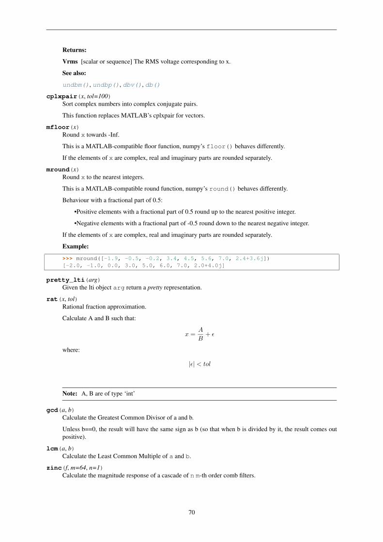
Returns:

Vrms [scalar or sequence] The RMS voltage corresponding to x.

See also:

undbm(), undbp(), dbv(), db()

cplxpair(x, tol=100)Sort complex numbers into complex conjugate pairs.

This function replaces MATLAB’s cplxpair for vectors.

mfloor(x)Round x towards -Inf.

This is a MATLAB-compatible floor function, numpy’s floor() behaves differently.

If the elements of x are complex, real and imaginary parts are rounded separately.

mround(x)Round x to the nearest integers.

This is a MATLAB-compatible round function, numpy’s round() behaves differently.

Behaviour with a fractional part of 0.5:

•Positive elements with a fractional part of 0.5 round up to the nearest positive integer.

•Negative elements with a fractional part of -0.5 round down to the nearest negative integer.

If the elements of x are complex, real and imaginary parts are rounded separately.

Example:

>>> mround([-1.9, -0.5, -0.2, 3.4, 4.5, 5.6, 7.0, 2.4+3.6j])[-2.0, -1.0, 0.0, 3.0, 5.0, 6.0, 7.0, 2.0+4.0j]

pretty_lti(arg)Given the lti object arg return a pretty representation.

rat(x, tol)Rational fraction approximation.

Calculate A and B such that:

𝑥 =𝐴

𝐵+ 𝜖

where:

|𝜖| < 𝑡𝑜𝑙

Note: A, B are of type ‘int’

gcd(a, b)Calculate the Greatest Common Divisor of a and b.

Unless b==0, the result will have the same sign as b (so that when b is divided by it, the result comes outpositive).

lcm(a, b)Calculate the Least Common Multiple of a and b.

zinc(f, m=64, n=1)Calculate the magnitude response of a cascade of n m-th order comb filters.

70

The magnitude of the filter response is calculated mathematically as:

|𝐻(𝑓)| =sinc(𝑚𝑓)

sinc(𝑓)

𝑛Parameters:

f [ndarray] The frequencies f at which the magnitude response is evaluated.

m [int, optional] The order of the comb filters.

n [int, optional] The number of comb filters in the cascade.

Returns:

HM [ndarray] The magnitude of the frequency response of the cascade filter.

71

72

Bibliography

[R1] P. Benabes, M. Keramat, and R. Kielbasa, “A methodology for designing continuous-time sigma-delta mod-ulators,” in Proc. Eur. Conf. Design Test, Washington, DC, 1997, pp. 46-50

[R2] J. Cherry and W. Snelgrove, “Excess loop delay in continuous-time delta-sigma modulators,” IEEE Trans.Circuits Syst. II, Analog Digit. Signal Process., vol. 46, no. 4, pp. 376-389, Apr. 1999

[R3] Shanthi Pavan, “Systematic Design Centering of Continuous Time Oversampling Converters”, IEEE Trans.on Circuits Syst. II Express Briefs, Volume.57, Issue 3, pp.158, 2010

73

74

Python Module Index

ddeltasigma.__init__, 1

75

76

Index

AaxisLabels() (in module deltasigma.__init__), 32

Bbilogplot() (in module deltasigma.__init__), 33bplogsmooth() (in module deltasigma.__init__), 34bquantize() (in module deltasigma.__init__), 34bunquantize() (in module deltasigma.__init__), 35

CcalculateQTF() (in module deltasigma.__init__), 37calculateSNR() (in module deltasigma.__init__), 35calculateTF() (in module deltasigma.__init__), 36cancelPZ() (in module deltasigma.__init__), 37changeFig() (in module deltasigma.__init__), 37circ_smooth() (in module deltasigma.__init__), 38circshift() (in module deltasigma.__init__), 39clans() (in module deltasigma.__init__), 39cplxpair() (in module deltasigma.__init__), 70

Ddb() (in module deltasigma.__init__), 40dbm() (in module deltasigma.__init__), 41dbp() (in module deltasigma.__init__), 41dbv() (in module deltasigma.__init__), 41delay() (in module deltasigma.__init__), 41deltasigma.__init__ (module), 1DocumentNTF() (in module deltasigma.__init__), 31ds_f1f2() (in module deltasigma.__init__), 41ds_freq() (in module deltasigma.__init__), 41ds_hann() (in module deltasigma.__init__), 42ds_optzeros() (in module deltasigma.__init__), 42ds_quantize() (in module deltasigma.__init__), 42ds_synNTFobj1() (in module deltasigma.__init__), 43dsclansNTF() (in module deltasigma.__init__), 43

EevalMixedTF() (in module deltasigma.__init__), 43evalRPoly() (in module deltasigma.__init__), 44evalTF() (in module deltasigma.__init__), 44evalTFP() (in module deltasigma.__init__), 44

FfigureMagic() (in module deltasigma.__init__), 45

frespF1() (in module deltasigma.__init__), 46

Ggcd() (in module deltasigma.__init__), 70

IimpL1() (in module deltasigma.__init__), 46infnorm() (in module deltasigma.__init__), 46

Ll1norm() (in module deltasigma.__init__), 47lcm() (in module deltasigma.__init__), 70logsmooth() (in module deltasigma.__init__), 47lollipop() (in module deltasigma.__init__), 48

MmapABCD() (in module deltasigma.__init__), 49mapCtoD() (in module deltasigma.__init__), 49mapQtoR() (in module deltasigma.__init__), 50mapRtoQ() (in module deltasigma.__init__), 51mfloor() (in module deltasigma.__init__), 70mod1() (in module deltasigma.__init__), 51mod2() (in module deltasigma.__init__), 51mround() (in module deltasigma.__init__), 70

NnabsH() (in module deltasigma.__init__), 51

Ppadb() (in module deltasigma.__init__), 52padl() (in module deltasigma.__init__), 52padr() (in module deltasigma.__init__), 52padt() (in module deltasigma.__init__), 52partitionABCD() (in module deltasigma.__init__), 53peakSNR() (in module deltasigma.__init__), 53PlotExampleSpectrum() (in module

deltasigma.__init__), 31plotPZ() (in module deltasigma.__init__), 54plotSpectrum() (in module deltasigma.__init__), 54predictSNR() (in module deltasigma.__init__), 55pretty_lti() (in module deltasigma.__init__), 70pulse() (in module deltasigma.__init__), 56

77

Rrat() (in module deltasigma.__init__), 70realizeNTF() (in module deltasigma.__init__), 57realizeNTF_ct() (in module deltasigma.__init__), 57realizeQNTF() (in module deltasigma.__init__), 58rms() (in module deltasigma.__init__), 59rmsGain() (in module deltasigma.__init__), 59

SscaleABCD() (in module deltasigma.__init__), 59simulateDSM() (in module deltasigma.__init__), 60simulateQDSM() (in module deltasigma.__init__), 61simulateQSNR() (in module deltasigma.__init__), 62simulateSNR() (in module deltasigma.__init__), 63sinc_decimate() (in module deltasigma.__init__), 64SIunits() (in module deltasigma.__init__), 32stuffABCD() (in module deltasigma.__init__), 64synthesizeChebyshevNTF() (in module

deltasigma.__init__), 65synthesizeNTF() (in module deltasigma.__init__), 66synthesizeQNTF() (in module deltasigma.__init__), 68

Uundbm() (in module deltasigma.__init__), 69undbp() (in module deltasigma.__init__), 69undbv() (in module deltasigma.__init__), 69

Zzinc() (in module deltasigma.__init__), 70

78