Embed Size (px)
Citation preview

Globalization and the spatial concentration of production
by
Friederike Niepmann and Gabriel J. Felbermayr
Nr.301/2008
ISSN 0930-8334

Globalization and the spatial concentration of production∗
Friederike Niepmann†and Gabriel J. Felbermayr‡
Oktober, 2008
Abstract
New trade theory models predict that freer trade increases the spatial concentration of
industrial production across countries. While nations with large home markets and cen-
tral geographical location become increasingly attractive business locations, small peripheral
countries gradually deindustrialize. Using data for 26 industries, 20 OECD countries and 20
years, we investigate the empirical validity of this claim. Separating out the role of home
market size from geographical factors, and using various panel methods, we find robust ev-
idence in line with theory. Freer trade has indeed magnified the importance of domestic
demand and geographical location for the pattern of industrial production across the globe
and has therefore exacerbated spatial disparities.
Keywords: Home market effect, hub effect, trade liberalization, trade costs, increasing re-
turns to scale, new trade theory, economic geography.
JEL-Codes: F12, F15
∗Parts of this paper were drafted when Niepmann was an intern at the World Bank. We are grateful to MaryAmiti, Michael Boehm, Matthieu Crozet, Benjamin Jung, Wilhelm Kohler, Andreas Kopp, and Davide Sala forcomments and discussion. All remaining errors are ours.
†Economics Department, European University Institute, Villa San Paolo, Via della Piazzuola 43, 50133 Flo-rence, Italy. E-Mail: [email protected].
‡Corresponding author. Economics Department (520E), Universitat Hohenheim, 70593 Stuttgart, Germany.E-mail: [email protected].

1 Introduction
Today’s general perception is that the world has moved closer together. Popular writers argue
that “the world is flat” (Friedman, 2005) or proclaim the “death of distance” (Cairngross, 1997).
While these claims are exaggerated, the academic literature (e.g., Hummels, 2007) leaves little
doubt that trade costs have indeed fallen. Progress in transportation technologies, such as
the introduction of containerization, or in communication technologies, e.g. the internet, and
substantial reductions in tariff and non-tariff barriers have greatly reduced barriers between
countries and have increased the freeness of trade. Indeed, the secular trend in trade costs
epitomizes what is usually meant by the buzzword “globalization”.
Virtually all mainstream trade theories predict that lower trade costs lead to welfare gains at
the global level. However, improved allocative efficiency notwithstanding, these aggregate gains
need not be evenly distributed within and across countries, so that there are losers and winners.
One recurrent worry of policy makers is that higher trade freeness spurs the deindustrialization of
small and peripheral countries and entrenches global inequality.1 This concern has a theoretical
foundation in trade models featuring increasing returns to scale at the firm level. ‘New Trade
Theory ’ (NTT) predicts that large and/or centrally located countries increasingly dominate the
production of industrial goods as trade costs fall.
Countries with large home markets are attractive places of production as firms want to save
on trade costs when servicing their largest customer base. The larger a country’s domestic
market, the disproportionately more firms it attracts. Increasing freeness of trade further boosts
this locational advantage, since it becomes cheaper to ship goods to foreign countries while
still selling to domestic consumers at no trade costs. The first channel has been described by
Krugman (1979) and Helpman and Krugman (1985). It is frequently referred to as the home
market effect (HME). However, geography matters, too. Central countries attract industrial
production since they allow cheap shipping to other countries; freer trade can magnify this
advantage. This second channel has been introduced by Krugman (1993) as the hub effect.
1The World Bank dedicates the forthcoming 2009 World Development Report “Reshaping Economic Geogra-phy” to the role of globalization in shaping spatial disparities.
2

In this paper we study empirically whether falling trade costs have indeed strengthened the
advantages of large and/or central countries as locations of industrial production. To this end,
we use 20 years of production and trade data for 20 OECD countries and 26 3-digit industries.
We build on the important work by Behrens, Lamorgese, Ottaviano and Tabuchi (2007), hence-
forth BLOT, who show how to empirically isolate the home market effect from confounding
geographical effects in a multi-country setup. We also use the concept of nominal market po-
tential, well established in the literature since Davis and Weinstein (2003), to quantify the joint
effect of the home market and the hub effect.
Our empirical results suggest that market size and geographical centrality have become more
important for the distribution of industrial production across countries, thereby contributing
to a stronger polarization of industrial activity over space and confirming concerns of policy-
makers. We find robust evidence for the decisive role of trade costs and show that both the
home market effect and the hub effect have gathered strength. Hence, evidence seems in line
with the predictions from NTT.2
The present paper is related to a large and growing literature. A number of authors study
changes in the industrial location and in specialization patterns across countries in episodes of
trade liberalization. Middelfart-Knarvik et al. (2000) as well as Amiti (1998, 1999) look at the
case of European integration, mainly focusing on concentration measures, such as the Herfindahl
index. Head and Ries (2001) study how the location of Canadian-U.S. manufacturing changed
as a reaction to the free trade agreement between Canada and the USA. That latter paper is
close to ours, in particular because it looks at the data through the lens of NTT. However, we
study a larger country sample (20 OECD countries) over a longer period of time (1988-1999)
and focus on technological change rather than tariff reform.
A number of papers argue that the HME is a distinctive feature of models with increasing
returns to scale and exploit this fact to assess the empirical success of those models as compared
to models featuring constant returns and other sources of product differentiation (e.g. Feenstra
2In other areas of research, empirical results are harder to square with the perceived evidence of falling tradecosts. For example, in gravity models, the trade-impeding influence of distance has grown stronger over time(Disdier and Head, 2008).
3

et al., 2001; Head et al., 2002). Although the HME does not need to appear in all theoretical
circumstances (see Davis, 1998, or Head and Mayer, 2004), it was found to be remarkably robust
to alternative specifications, such as linear demand and per unit transportation costs (Ottaviano
et al. (2002)), heterogeneous firms (Okobu and Rebeyrol, 2006) and even to the departure from
the Dixit-Stiglitz monopolistic-competition structure (Holmes and Stevens, 2005). Davis and
Weinstein (2003), Feenstra et al. (2002), Hanson and Xiang (2004) as well as Brulhart and
Trionfetti (2007) have found empirical support for HMEs in differentiated goods industries.
Head and Ries (2001), who exploit time variation, find mixed evidence for industrial relocation
in line with NTT.3 Our paper differs form earlier approaches in that it tries to assess the evolution
of the HME over time.
A central complication with the empirical identification of the HME arises when there are
more than two countries and asymmetric trade costs across country pairs – the natural situation
in many empirical studies. In that case, the hub effect confounds the HME. BLOT recently
generalized the standard model to the multi-country setup with asymmetric trade costs. They
show that the effect of changes in market size on industry location is different for differently
located countries and depends on trade barriers with and of all countries and simultaneous
demand shifts in the entire world. In our exercise, we apply the theory-based linear filter
suggested by BLOT, which separates out the pure HME by correcting the data for effects from
asymmetric trade costs and geography. However, since we are interested in the total effect of
falling trade costs on industrial location, we also relate changes in production to changes in
nominal market potential (NMP), a combined measure for a country’s attraction (attributed to
its market size) and accessibility (related to its geographical location). Interestingly, across all
our specifications we find that freer trade has made the distribution of industrial production
spatially more concentrated.
The remainder of this paper is structured as follows. Section 2 considers the theoretical
mechanisms that link the distribution of industrial production to market sizes and geographical
location. Section 3 discusses the empirical strategy and presents the data together with evidence
3For a summary on the HME literature, see Head and Mayer (2004).
4

on trade costs. Section 4 shows our main results. Section 5 presents caveats, robustness checks
and additional results. Section 6 concludes.
2 What determines the international distribution of firms?
2.1 Setup
In this section, we describe the mechanisms through which the size of nations and their relative
geographic position determines their importance as locations of industrial production. For that
purpose, a setup with two sectors and three countries proves sufficiently general.4
There are two goods: a costlessly tradable outside (agricultural) good, and a differentiated
(industrial) good which comes in a continuum of varieties. The outside good is typically produced
under perfect competition and constant returns to scale, while variants of the differentiated good
are produced by identical monopolistically competitive firms. Production involves fixed costs,
but marginal costs are constant. There is only one factor of production: labor. Assuming that
all countries produce both types of goods, they share the same wage rate, which we normalize
to unity.5 Countries are indexed by i, with i ∈ {1, 2, 3} . They may differ with respect to the
size of their labor force Li and their geographical location, but are otherwise perfectly identical.
Preferences of the representative consumer are such that the elasticity of substitution between
varieties (and hence the elasticity of demand) is parametrically given by σ > 1. Hence, monopoly
markups are constant. Welfare W (i.e., the real wage) is then just inversely proportional to the
ideal price level Pi.
Each differentiated variety is produced by a single firm and sold in all countries. Firms
charge monopoly markups, but equilibrium profits are zero due to free entry and exit. In this
theoretical setup all firms have equal size and charge identical ex-factory prices, see Feenstra
4Our analysis is based on BLOT, who generalize the Helpman and Krugman (1985) model to the asymmetricmulti-country multi-sector case. The special case of the BLOT model with two sectors and three countries hasbeen studied in deep detail by Sudekum (2007).
5Factor price equalization (FPE) is crucial, see Davis (1998) and the recent paper by Crozet and Trionfetti(2008) for the two-country case. Constant returns to scale and perfect competition in the outside good sector are,however, only sufficient conditions for FPE. Also note that FPE is not necessary for qualitative results discussedin this paper.
5

(2004) for a textbook treatment. Intranational trade is not affected by trade costs; international
shipments from country i to j, however, require costly transportation so that imported varieties
are by a factor τij ≥ 1 more expensive than domestic ones. Trade volumes between i and j are
proportional to the freeness of trade between countries i and j, φij ≡ τ1−σij , with φij ∈ (0, 1] ,
where φij = 1 corresponds to entirely free trade and a value of φij close to 0 implies prohibitively
large trade costs. Domestic sales and profits are unaffected by trade costs. Export sales and
associated profits, however, rise with φ since exporters are more competitive.
2.2 The role of country size and location
Denote by λi the share of country i in global production of the differentiated good and by θi its
share in total world population. Since all firms have equal size in the model, λi also measures the
distribution of firms across countries. Ruling out trade imbalances, θi measures the distribution
of expenditure (equal to income and home market size) across countries. In the following, we
illustrate the role of increasing freeness of trade in shaping the link between the distribution of
population θi and that of industrial production λi and investigate whether that relationship has
changed systematically as trade has become freer. More precisely, we care about the value and
determinants of b in6
λi = bθi. (1)
For a start, assume that all countries have equal populations L1 = L2 = L3 and there are no
differences in the bilateral freeness of trade across country pairs so that φij = φ ∈ (0, 1] . In this
perfectly symmetric situation, economic outcomes must be symmetric, too: the differentiated
goods sector is of equal size in all countries. Trade is exclusively intra-industry, and welfare
levels are equalized.
The home market effect (HME). Now assume that country 3 becomes larger, everything
else equal, so that its share in total world population goes up while that of the other countries
6This equation is a simplification: with many asymmetric countries, it features a constant term (see BLOT);in more general setups it may not be log-linear (Crozet and Trionfetti, 2008).
6

falls: ∆θ1 < 0,∆θ2 < 0,∆θ3 > 0. Panel (a) in Figure 1 offers an illustration. In this case one
obtains b > 1 in equation (1), which indicates that the larger country attracts an overpropor-
tionally large share of firms. To understand this, let us assume the contrary, i.e., b = 1. Then,
the distribution of firms and that of population coincide and λi = θi for all i = 1, 2, 3. Is this
an equilibrium?
φ φ
1
2 3 φ
(a) Pure HME
2φ 2φ
1
2 φ3
(b) Pure Hub Effect
2φ 2φ
1
2 φ3
(c) HME and Hub Effect confounded
Figure 1: Market size and trade costs in the three-country world.
In an equilibrium, firms cannot further increase their profits by changing location from one
country to the other. This is, however, not the case in the situation described above. Firms in
country 3 face a larger share of demand from their home country than from abroad, because the
home country is bigger. Moreover, that share of demand is completely exempt from trade costs
so that profits stemming from domestic sales are bigger. If b = 1, demand per firm in country 3
would be larger than elsewhere; associated profits would be, too. It follows that firms relocate
from the (symmetric) countries 1 and 2 into 3. The concentration of firms leads to market
crowding in 3, so that firms’ sales and profits decline. In the small countries, the converse is
true. This mechanism balances profit opportunities across the two countries. Hence, b = 1 is
not an equilibrium, neither is b < 1 as profits would diverge further. Hence, b > 1 must hold.
This is the home market effect (HME). It implies that an increase in a country’s expenditure
share causes an overproportional expansion in its share of firms. This is equivalent to stating
that country 3 is a net exporter of the differentiated good while the other countries are net
importers. Moreover, welfare is higher in country 3 (W3 > W1 = W2), since a smaller share of
total consumption is burdened by trade costs, leaving the consumer price index lower than in
the other countries.
7

If there were simultaneous changes of Li in all countries, for example ∆L1 > ∆L2 > ∆L3,
the home market effect would prevail in each pairwise comparison of countries. Countries could
then be ranked with respect to their share of production relative to population: λ1/θ1 > λ2/θ2 >
λ3/θ3.
The hub effect. Now, we revert to identical country sizes but assume that country 1 enjoys
easier access to the markets of its trading partners 2 and 3 than those partners between them.
For the sake of concreteness, φ12 = φ21 = φ13 = φ31 = φ2 < φ, while φ23 = φ32 = φ. Panel
(b) in Figure 1 illustrates this case. Country 1 has a central geographic location, or it may
have concluded special trade agreements with its partners. In this situation, is λi = θi for all
i ∈ {1, 2, 3} an equilibrium? As above, the answer is no. However, the reason is different.
On average, exporters in country 1 are less strongly affected by trade costs than exporters in
countries 2 and 3 are. This implies that firms in country 1 serve consumers in country 2 (or
3) at lower prices than firms based in country 3 (or 2). Hence, λi = θi is incompatible with
equality of profits across countries, and firms have incentives to reallocate. It follows that in
equilibrium λ1 > θ1, while λ2 < θ2 and λ3 < θ3. Country 3’s central geographical location
makes it attractive for firms to locate there. Firms export their output at low costs to the
other countries, thereby turning country 3 into a net exporter of differentiated goods. This is
the hub effect first discussed by Krugman (1993). Countries 2 and 3 are net exporters of the
homogeneous good, which is costlessly tradable, and where geographical disadvantage does not
matter. Welfare is larger in the central country 1 (W1 > W2 = W3) because a lower share of
total consumer spending is affected by trade costs.
HME and hub effect combined. We can now turn to panel (c) in Figure 1. Starting from
the situation of asymmetric trade costs described in panel (b), we study the effect of an increase
in market size of country 3. Now, the HME in country 3 is confounded by the hub effect in
country 1. It is no longer obvious that an increase in the relative size of country 3 more than
proportionally boosts its share of industrial production. The reason is that the larger market
size of country 3 also increases the attractiveness of country 1 thanks to its role as a preferred
8

location for exporters. Clearly, the strength of this effect depends on the size of trade costs
between 1 and 3. It is possible that the new equilibrium features λ1 > θ1,λ2 < θ2, and λ3 ≥ θ3.
Hence, the hub effect confounds the HME and there need not be a clear relation between changes
in own market size and industrial production any more.
BLOT provide a numerical 3-country example where all countries differ with respect to size
and geography and in which the HME is dwarfed by the hub effect so that the larger country
actually has a lower share of firms than the medium-sized country. They show that the hub
effect dominates when trade impediments are sufficiently high and country sizes not too different.
Note, however, that the hub effect can also enforce the market size effect, for example, if the
large country happens to be the central one (unlike in our figure).
2.3 The role of higher freeness of trade
For a given level of trade costs, industrial production concentrates in large and/or central coun-
tries. Does freer trade, e.g., due to improvements of transport technology, lower communication
costs, or tariff reform exacerbate the spatial disparities or attenuate them?
The home market magnification effect (HMME). First, we focus on a situation where
countries differ only with respect to size and trade becomes uniformly freer across all country
pairs. This makes the HME stronger, thereby making the distribution of industrial production
across countries more skewed. The theoretical result ∂b/∂φ > 0 is known as the home market
magnification effect (HMME). The intuition is the following. As long as trade is not entirely
costless, i.e., φ < 1, producing in the larger country remains advantageous, as a larger share of
local firms’ total sales remains untouched by international trade costs. Higher freeness does not
alter this effect. However, the benefits of concentrating production in the larger country have
gone up since serving the other countries through exports is now cheaper. Hence, incentives to
locate in the larger market have become stronger.
One can also highlight the HMME by starting from the extreme case, where trade is entirely
frictionless, i.e., φ = 1. Then, exporting does not come with additional costs, so that varieties sell
9

at the same price and firms make the same profits in all markets regardless of where they produce
and sell (as long, of course, as countries still produce both the outside and the differentiated
good). Hence, the distribution of firms across countries becomes essentially indeterminate. A
proportional distribution of firms over countries is therefore a possibility, even if countries differ
in size. However, the tiniest deviation from free trade would induce a massive reallocation
of firms towards the largest country. This is so because sales to that country generate the
largest share of firms’ profits, so that firms benefit by locating there in order to save trade costs.
However, since freeness of trade is still almost perfect, exporting to the rest of the world causes
little profit losses.
The hub magnification effect. The hub effect can also be magnified when the freeness of
trade goes up. Using panel (b) of Figure 1, any improvement in φ has a stronger effect for the
country pairs that involve the central country 1 than for the other pairs. Hence, the locational
advantage of country 1 becomes stronger, it attracts even more industrial firms, and fortifies
its role as a hub. As a consequence, the distribution of industrial production across countries
becomes more skewed.
Figure 1 is constructed such that a change of φ affects country pairs asymmetrically, which
strengthens the peripherality of countries 2 and 3. However, even if trade costs τij fall pro-
portionally in all pairs, so that the relative freeness of trade φij/φkl remains unchanged, the
hub effect is magnified. Krugman (1993) shows that “we expect concentration of production
in transportation hubs when transportation costs are low, rather than when they are high” (p.
35). To see this, suppose that in some initial situation trade is entirely free (φij = 1) . Hence, it
is possible that the distribution of production is proportional to country sizes. If there are small
impediments to trade between countries 1 and 2 (φ12 = φ21 < 1) , there is strong relocation of
firms towards country 1, because trade costs can be fully avoided by producing there. If initially
countries are in autarky (φij = 0) , production is also evenly distributed. When trade costs
involving country 1 rise to a small positive number, then country 1 becomes a hub. However,
relocation is weak, since trade costs are still almost prohibitive. Hence, the hub effect is stronger,
when the overall level of trade costs is low.
10

Summary. In the context of a very general setup, Behrens et al. (2004) show that the spatial
distribution of production becomes generally more uneven with increasing trade freeness when
both forces interact, while geography becomes relatively more important for the location of
production compared to market size.7 In a globalizing world, we therefore expect industrial
production to move towards locations where domestic markets are large and from which trade
with other markets is easy, while geography should increasingly gain weight as a determining
factor. New trade theory therefore predicts that the cross-country distribution of industrial
production increasingly decouples from the distribution of population. In the following empirical
exercise we show that this decoupling has indeed occurred.
However, it is important to note that the implications for cross-country welfare differences
are non-monotonic. Clearly, as soon as the freeness of trade is total, the location of production
does not have any relevance on welfare since aggregate price levels and nominal income are
both equalized across countries. However, when the freeness of trade is sufficiently low to start
with, a further increase in trade freeness may increase global disparities, therefore justifying
wide-spread policy concerns.
3 Empirical implementation
Equation (1) has a natural empirical counterpart
λikt = α+ βθit + εikt, (2)
where λikt is the production share of country i in industry k at time t, θit is the overall demand
share for industrial goods of country i at time t, α is a constant, and εikt is an i.i.d. error
term. We will follow the literature8 and use data on value-added to proxy production shares.
Demand shares are based on national absorption, the residual between output and net trade.9
7See Proposition 2 in Behrens et al. (2004), p.14.
8Some of the most important recent empirical studies are Crozet and Trionfetti (2008), Behrens et al. (2007),Davis and Weinstein (2003) and Head and Ries (2001).
9For the exact calculation of the different variables as well as data sources, see the Data Appendix.
11

Traditionally, empirical studies run equations of the type stated above in a cross-section and test
whether β > 1, which is understood as a test for the existence of an HME. In this study, we use
three different theory-inspired specifications, which differ with respect to the exact definitions
of the production and demand shares used in equation (2); see Table 1.
Table 1: Production-demand specifications
θobserved θNMP
λfilter HME –
λobserved Naive HME+Hub
The HME specification. As argued in Section 2, in a multi-country world with asymmetric
trade costs, the hub effects confounds the HME. However, BLOT offer an elegant way to isolate
the effect of pure size effects. To that purpose, they propose a linear filter, which corrects the
observed production shares λikt year-by-year for asymmetric trade costs. Filtering yields those
production shares λfilterikt that one would observe if trade costs were symmetric across countries.
Using filtered production shares allows identifying the HME by running Equation (2). We call
this first production-demand specification HME specification, which uses λfilterikt and θobservedit to
estimate Equation (2). β > 1 indicates the presence of the HME, while a positive dependence
of the parameter on the degree of trade freeness would reveal the home market magnification
effect (HMME).
The HME+Hub specification. Beyond the HME and HMME, we are also interested in
the hub effect and the importance of geography. In particular, we want to know whether they
are augmented by rising trade freeness. However, measuring the hub effect in isolation from
the home market effect is not feasible. Changes in the global trade cost structure, e.g. in
form of bilateral free trade agreements or improved infrastructure, are unlikely to have a clearly
measurable impact on industry location over time. This would be necessary to measure the hub
effect separately in a similar fashion to the HME. However, we can use an intuitive measure,
12

namely nominal market potential (NMP), well known in the related literature, to measure the
joint impact of the HME and the hub effect on industry location.10 A country’s nominal market
potential is the sum of its domestic demand and distance-weighted demands of all other countries
and thus captures a country’s attractiveness due to both forces, market size and accessibility.
We construct θNMPit as a country’s share in world NMP (the sum of NMP over all countries)
and thereby measure a country’s attractiveness as a business location relative to others. The
production share will be proxied by the observed production share in terms of value added,
λobservedikt . We call the specification the HME+Hub specification. Using θNMPit in Equation (2)
and testing for β > 1 would not be informative about the HME or hub effect per se. Nevertheless,
this specification will reveal whether firms, as we expect, locate predominantly in countries with
a high share in NMP, and whether they concentrate more and more in those comparatively
attractive places when trade costs fall.
NMP does not take into account differences in prices and may therefore overestimate the
market potential of large markets and underestimate it for small ones. However, as turns out,
the use of NMP is unproblematic for our exercise. Overestimation of NMP for large markets
would bias the estimated slope of the line relating the production to the demand shares down-
wards, hence stacking the cards against the predictions of theory. If we do find disproportionate
responses between demand and production, then they must be sufficiently strong in the data to
still show up econometrically despite the bias in NMP.
Naive specification. As a third specification, which we call Naive specification, we regress
the unfiltered production shares λobservedikt on uncorrected demand shares θobservedit . This allows
to see, how the filter helps to detect the HME, which in this specification is distorted by effects
from asymmetric trade costs.
Some notes on the data. Our data covers twenty years, from 1980 to 1999, 20 OECD coun-
tries, and 26 three-digit ISIC industries. The country coverage is common to the literature,
10Davis and Weinstein (2003) as well as Crozet and Trionfetti (2008) account for geography by measuringdemand in terms of nominal market potential (NMP) when taking the Helpman and Krugman (1985) model tothe data.
13

see Hanson and Xiang (2004) or BLOT. It has the advantage that countries have similar tech-
nologies and tastes which is assumed in the theory. Moreover, they share comparable access to
international factor markets, which should minimize the role of comparative advantage. Also
the level of industry disaggregation is standard in the literature, see Davis and Weinstein (2003),
Hanson and Xiang (2004), Crozet and Trionfetti (2008), BLOT.11 The units of analysis in our
exercise are country (i) × industry (k) pairings observed over time (t). There are, therefore a
maximum of 20 × 26 × 20 = 10, 400 observations, from which we actually observe about 83%
(N = 8, 679).12
3.1 Freeness of trade
The motivation of our analysis rests on the presumption that trade costs have fallen over time,
i.e., that the freeness of trade has increased. In addition to anecdotal evidence, we draw on
data to check whether the expected evolution of trade costs and the freeing up of trade can be
confirmed by our data.
We use a narrow and a broad measure of trade freeness. The narrow measure φnarrowkt is
based on freight rate data from Bernard et al. (2006) and has an industry×time dimension.
This measure captures changes in the freeness of trade solely driven by variation in freight rates
over industries and over time. It suffers from the fact that it excludes other types of trade costs.
Therefore, we provide a broad measure φbroadkt , which can be calculated from bilateral trade data
and which accounts for all types of trade costs. The shortcoming of this indicator is that it
is a non-linear function of the elasticity of substitution. If the latter varies over time, φbroadkt
confounds changes in trade costs over time with changes in preferences, which have nothing to
do with the freeness of trade as it is commonly understood.13
Figure 2 shows the evolution of the narrow and the broad measure of trade freeness for
11Davis and Weinstein (2003) discuss the role of aggregation. It is not immediately clear, which level ofaggregation is most appropriate to meet the underlying assumptions on varieties and goods. In the theoreticalmodel, industries are categorized by factor inputs rather than by product usage as is the case for ISIC industries.
12For summary statistics, see Table 9 in the Data Appendix.
13For the exact calculation of our measures, see the Data Appendix.
14

homogeneous and heterogeneous industries over time. Industries are categorized following Lyons
and Sembenelli (1997). Both measures indicate that the freeness of trade has increased from
1980 to 1999. In our empirical analysis, we will interpret time variation in the average freeness
of trade as changes in trade costs rather than preferences. Figure 2 underlies this argumentation
as it features a very similar evolution for both the narrow and broad measures as well as for
both groups of industries, heterogeneous and homogeneous.
Figure 2: Evolution of freeness of trade for homogeneous and heterogeneous industries
4 Results
4.1 The HME
Before analyzing the role of increasing trade freeness for the spatial distribution of production,
we check for evidence for the HME and/or the hub effect in our data. This allows to relate
our analysis to the existing literature and to compare the performance of the three production-
demand specifications. In the spirit of Head and Ries (2001), we conduct “within” and “between”
regressions, the former exploiting the time-variation including country-industry fixed effects and
the latter drawing on the cross-sectional variation in the data.
Columns (1)-(3) of Table 2 show within estimates for our three specifications; columns (4)-(6)
present the results for between regressions using weighted least squares in order to account for
the unbalanced panel. The slope coefficient β from Regression (2) is our parameter of interest,
where β > 1 indicates a more than proportional response of production to the different demand
15

Table 2: Testing for overproportional response.
Dep.var.: Production share λWithin estimates Between estimates
(1) (2) (3) (4) (5) (6)Naive HME HME+Hub Naive HME HME+Hub
Demand share θ 0.971∗∗∗ 1.588∗∗∗ 0.808∗∗∗ 1.053∗∗∗ 1.252∗∗∗ 1.359∗∗∗
(0.0173) (0.350) (0.0209) (0.0146) (0.0443) (0.0208)
R2 within 0.278 0.003 0.154 0.278 0.003 0.154R2 between 0.889 0.311 0.870 0.910 0.608 0.892R2 overall 0.878 0.074 0.851 0.878 0.074 0.851Standard errors in parentheses. ***, **, * refer to p<0.01, p<0.05,p<0.1.8679 observations for all six regressions. Constant not reported.Within regressions include country-industry fixed effects. Between regressions use weighted least squares.Naive specification uses uncorrected variables. HME specification includes filtered production shares.HME+Hub specification captures demand shares in terms of nominal market potential.
measures. Results differ across specifications and econometric methodologies. Within estimates
only signal a disproportionate reaction of the production share for the HME specification, but
not for the naive or the HME+hub specification. The failure to find evidence for the HME in the
within model is in line with Head and Ries (2001). Coefficients from the naive specification also
roughly correspond to their estimates for the slope coefficient. However, our analysis suggests
that correcting the production data for geographical differences, as BLOT recommend, confirms
the existence of an HME even in the within analysis. This is an interesting result, which points
towards the overall usefulness of the methodology proposed by BLOT.
Evidence from the between regressions, which exploit the cross-sectional variation of the
data, yields more consistent results. This is in line with much of the literature; Feenstra et al.
(2001), Davis and Weinstein (2003), Hanson and Xiang (2004) and BLOT find that countries
with large domestic markets produce disproportionately more differentiated goods than smaller
countries, while the presence and the magnitude of the HME seem to be positively related to
the degree of industry differentiation.
At this stage, we conclude that the evidence for disproportionate reactions of production
shares to different measures of demand shares is mixed, except when the analysis is narrowed
16
down to the pure HME. However, in this paper, we are mainly interested in understanding the
behavior of β as trade becomes freer.
4.2 Magnification effects
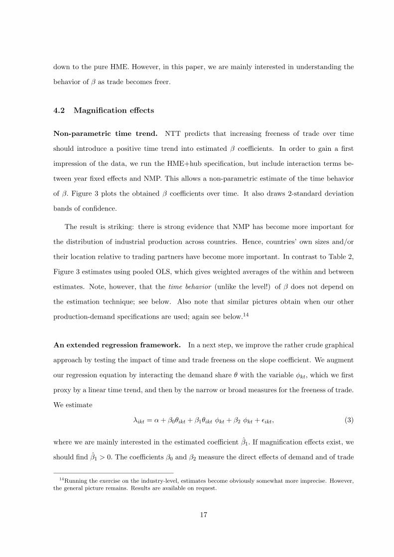
Non-parametric time trend. NTT predicts that increasing freeness of trade over time
should introduce a positive time trend into estimated β coefficients. In order to gain a first
impression of the data, we run the HME+hub specification, but include interaction terms be-
tween year fixed effects and NMP. This allows a non-parametric estimate of the time behavior
of β. Figure 3 plots the obtained β coefficients over time. It also draws 2-standard deviation
bands of confidence.
The result is striking: there is strong evidence that NMP has become more important for
the distribution of industrial production across countries. Hence, countries’ own sizes and/or
their location relative to trading partners have become more important. In contrast to Table 2,
Figure 3 estimates using pooled OLS, which gives weighted averages of the within and between
estimates. Note, however, that the time behavior (unlike the level!) of β does not depend on
the estimation technique; see below. Also note that similar pictures obtain when our other
production-demand specifications are used; again see below.14
An extended regression framework. In a next step, we improve the rather crude graphical
approach by testing the impact of time and trade freeness on the slope coefficient. We augment
our regression equation by interacting the demand share θ with the variable φkt, which we first
proxy by a linear time trend, and then by the narrow or broad measures for the freeness of trade.
We estimate
λikt = α+ β0θikt + β1θikt φkt + β2 φkt + εikt, (3)
where we are mainly interested in the estimated coefficient β1. If magnification effects exist, we
should find β1 > 0. The coefficients β0 and β2 measure the direct effects of demand and of trade
14Running the exercise on the industry-level, estimates become obviously somewhat more imprecise. However,the general picture remains. Results are available on request.
17

Figure 3: Increasing HME+Hub effect over time
freeness on production shares.
Linear time trend. Table 3 reports output for the estimation of Equation (3) when a linear
time trend captured by our variabel time is used as proxy for φkt.15 Columns (1) to (3) display
results from a pooled OLS regression; columns (4) to (6) show within estimates. We find
evidence for a positive time trend in the slope coefficient. All estimates of the coefficients
β1 are positive. The estimates for the slope coefficients β0 remain mainly in line with the
estimates from the previous within regression from the pooled sample. The time trend for the
HME+hub specification is more pronounced than for the HME version. Using, e.g., column (6),
our estimates imply that the estimated ∂λ/∂θ is 0.925 in 1980 and 1.312 in 1999. This is a
very substantial increase. Regarding columns (2) and (5), where geographical effects are fully
sterilized, there is a positive time trend, too, but it is not statistically significant at standard
levels of confidence. However, the estimated β0 is already fairly large to start with.
Magnification effects and the freeness of trade. We can further improve our analysis by
directly exploiting the time variation of measured trade freeness on the industry level. For this
purpose, we use Equation (3), and substitute φnarrowkt or φbroadkt . Since the broad measure has
15time = 0.01 (year − 1979) .
18

Table 3: Time trends and the demand-production nexus
Dep.var.: Production share λOLS estimates Within estimates
(1) (2) (3) (4) (5) (6)Naive HME HME+Hub Naive HME HME+Hub
Demand share θ 0.958∗∗∗ 1.180∗∗∗ 1.128∗∗∗ 0.921∗∗∗ 1.547∗∗∗ 0.905∗∗∗
(0.020) (0.074) (0.025) (0.017) (0.353) (0.020)
time× θ 0.909∗∗∗ 0.766 2.245∗∗∗ 0.924∗∗∗ 0.762 2.034∗∗∗
(0.186) (0.753) (0.245) (0.041) (0.845) (0.061)
time −0.048∗∗∗ −0.046 −0.122∗∗∗ −0.049∗∗∗ −0.051 −0.108∗∗∗
(0.006) (0.078) (0.009) (0.004) (0.090) (0.005)
R2 within − − − 0.321 0.003 0.256R2 between − − − 0.889 0.311 0.871R2 overall 0.880 0.074 0.859 0.880 0.074 0.859Standard errors in parentheses. ***, **, * refer to p<0.01, p<0.05,p<0.1.8679 observations for all six regressions. Constant not reported.Within regressions include country-industry fixed effects. OLS regressions include industry dummies and showrobust standard errors.The variable time is a measure for the time trend. Naive specification uses uncorrected variables. HMEspecification includes filtered production shares. HME+Hub specification captures demand shares in terms ofnominal market potential.
been used to construct the independent variable θNMPikt in the HME+Hub specification, and the
dependent variable λfilterikt in the HME specification, using the same measures of trade freeness in
the interaction terms may seem problematic. However, this is hardly the case for the HME+Hub
specification. An average decline in the degree of freeness does not affect the demand shares
constructed from NMP at all. Changes in the share are really induced by bilateral changes
in trade costs and thus by shifting weights, so that θNMP does not contain information about
the level of trade freeness. Problems from collinearity simply do not emerge. With regard to
the filter, the mechanisms are more complicated because it is the independent variable which is
manipulated. As the filtered production share is a function of the entity of bilateral trade costs,
it may be inappropriate to include it on the right-hand side of the equation. Even though we
are aware of this problem, we report results for this specification in order to be complete. In any
case, no problem exists for the naive specification. Although it does not account for geography
19

effects, the magnification effect should be observable, if domestic expenditure is an increasingly
important determinant for production. These issues do not arise when we use freight rates, since
they have not been used to correct either θikt or λikt.
Panel A in Table 4 reports our results when the demand share is interacted with the narrow
measure of trade costs (i.e., freight rates). Across specifications and in both the within and the
between models we find positive coefficients of the interaction term φnarrow × θ. They are large,
because trade costs are measured at low scale. With the exception of the HME specification in
column (2), the obtained coefficients are highly statistically significant, signaling the existence
of magnification effects.
Panel B repeats the exercise, using the broad definition of trade freeness φbroad instead of the
narrow one. Here, we find for every single specification and both econometric models that freer
trade magnifies the effect of demand shares on the distribution of production. Our preferred
specification is the one shown in column (3) of panel B, where time variance is used to identify
the magnification effect based on NMP. Here, evaluating ∂λ/∂θ at the lowest realization of φbroad
yields an estimate of 0.796 while at the highest realization we have 1.234. Again, this is a very
substantial difference.
It is remarkable that the signs of the interaction terms and the magnitude of the coefficients
are consistent for the within and between regressions. Head and Ries (2001) find reversed signs
for the coefficients obtained from the within regressions (positive coefficient for the interaction
of the expenditure share with trade costs). Here, the picture from the different regression
exercises is unambiguous: lower trade freeness (i.e., higher freight rates), clearly decreases the
responsiveness of the production share to changes in the demand share. The findings thus
explicitly fit our expectations from theory and support the link between production and demand
predicted by NTT.
20

Table 4: Freeness of trade and the demand-production nexus
Dep.var.: Production share λPanel A: Narrow measure
Within estimates Between estimates(1) (2) (3) (4) (5) (6)
Naive HME HME+Hub Naive HME HME+Hub
Demand share θ 0.805∗∗∗ 1.492∗∗∗ 0.565∗∗∗ 0.817∗∗∗ 0.564∗∗∗ 1.059∗∗∗(0.020) (0.40) (0.023) (0.042) (5.98) (0.061)
φnarrow × θ 9.599∗∗∗ 5.556 18.19∗∗∗ 11.62∗∗∗ 33.97∗∗∗ 14.88∗∗∗(0.57) (11.7) (0.86) (1.96) (5.98) (2.86)
φnarrow −0.518∗∗∗ −0.420 −0.977∗∗∗ −0.625∗∗∗ −1.836∗∗∗ −0.796∗∗∗(0.061) (1.26) (0.073) (0.20) (0.62) (0.24)
R2 within 0.302 0.003 0.200 0.302 0.002 0.189R2 between 0.894 0.314 0.871 0.916 0.631 0.897R2 overall 0.884 0.075 0.857 0.885 0.076 0.860Panel B: Broad measure
Within estimates Between estimates(1) (2) (3) (4) (5) (6)
Naive HME HME+Hub Naive HME HME+Hub
Demand share θ 0.956∗∗∗ 1.265∗∗∗ 0.795∗∗∗ 0.947∗∗∗ 0.743∗∗∗ 1.226∗∗∗
(0.017) (0.352) (0.021) (0.022) (0.062) (0.031)
φbroad × θ 0.844∗∗∗ 18.91∗∗∗ 1.470∗∗∗ 5.154∗∗∗ 24.81∗∗∗ 6.520∗∗∗
(0.132) (2.658) (0.185) (0.809) (2.306) (1.165)
φbroad −0.050∗∗∗ −1.175∗∗∗ −0.084∗∗∗ −0.283∗∗∗ −1.460∗∗∗ −0.343∗∗∗
(0.015) (0.306) (0.018) (0.087) (0.249) (0.104)
R2 within 0.282 0.009 0.161 0.916 0.680 0.898R2 between 0.891 0.344 0.874 0.225 0.008 0.145R2 overall 0.880 0.087 0.855 0.880 0.088 0.854Standard errors in parentheses. ***, **, * refer to p<0.01, p<0.05,p<0.1.8679 observations for all six regressions. Constant not reported.Within regressions include country-industry fixed effects. Between regressions use weighted least squares. .Naive specification uses uncorrected variables. HME specification includes filtered production shares.HME+Hub specification captures demand shares in terms of nominal market potential.φnarrow is our narrow measure for the freeness of trade calculated from underlying data on industry-specific freightrates. φbroad is the broader measure for the freeness of trade constructed from data on bilateral exports capturingall kind of impediments to trade.
21

Figure 4: Share of considered countries in total world demand and value-added
5 Caveats, robustness checks and additional results
5.1 Caveats
Rest of the world. One objection to our analysis may be that developments outside of our 20-
country world–let us call them “rest-of-the-world” (ROW) effects–may drive results. However, it
is difficult to anticipate how changes in the ROW should systematically influence the relationship
of the production and the demand shares. One scenario is conceivable: Growing demand in the
ROW could lead to increased production in some of the 20 countries, so that production relocates
independent from changes in the distribution of demand among countries included in the sample.
If in addition demand shifts in the same direction as production, then the regression will yield
a high positive estimate for the slope coefficient, which is interpreted as HME, although it is
entirely due to effects in the ROW. There may even be an endogeneity problem if domestic
demand increases due to increased foreign demand, which would, in turn, bring with it higher
domestic production and income. In order to investigate what happens in the ROW over time,
we calculate the share of the 20 countries included in the dataset in world manufacturing using
the complete set of 183 countries contained in the original production dataset provided by Mayer
and Zignago (2005). Figure 4 shows a steady decline in the demand and production shares, while
both shares move more or less in parallel. If some production and demand shifts similar to the
22

described scenario would be responsible for the time trend, we would expect to see diverging
demand and production shares. If anything, the figure could be interpreted as support for NTT.
It indicates that the gap between the production share and the demand share increases in the
middle of the nineties. Therefore production seems to react over-proportionately to demand at
this point.
Table 5: Instrumental variable regressions
Dep.var.: Production share λ(1) (2) (3)
Naive HME HME+Hub
Demand share θ 0.908∗∗∗ 1.150∗∗∗ 0.968∗∗∗
(0.0447) (0.164) (0.0480)
time× θ 1.365∗∗∗ 0.980 2.866∗∗∗
(0.356) (1.231) (0.287)
time −0.0720∗∗∗ −0.0467 −0.158∗∗∗
(0.0140) (0.140) (0.0115)
R2 0.874 0.061 0.862Standard errors in parentheses. ***, **, * refer to p<0.01,p<0.05,p<0.1.6217 observations for all six regressions. Constant not reported.The demand shares are instrumented with 5-year lags.The variable time is a measure for the time trend. Naive specificationuses uncorrected variables. HME specification includes filtered pro-duction shares. HME+Hub specification captures demand shares interms of nominal market potential.
Simultaneity bias. A general problem is simultaneity bias. When current production is
regressed on current demand, simultaneity can arise from contemporaneous correlations as in-
dustry shocks may equally affect the production and the demand side. However, as absorption
is overall demand for differentiated goods constructed as residual between the total value of
production and net trade, whereas production is industry-specific value-added, this problem
should not be too severe. Moreover, measurement errors affecting the production and the de-
mand variables at the same time could lead to biased results. Yet if this was the case, β0 and
β1 would be biased downwards, which for our purpose of testing β0 > 1 and β1 > 0 should not
23

harm conclusions either.16 To mitigate simultaneity concerns, we instrument demand by lagged
values and run instrumental variable regressions. Table 5 reports results for 5-year lags. The
instrumental variable regression shows a similar picture as Table 3, while the time trend in the
slope coefficient is even more pronounced with slightly higher estimates for β1.
5.2 Other robustness checks
Table 6: Industry-specific demand shares
Dep.var.: Production share λOLS estimates Within estimates
(1) (2) (3) (4) (5) (6)Naive HME HME+Hub Naive HME HME+Hub
Demand share θ 0.994∗∗∗ 1.240∗∗∗ 1.126∗∗∗ 0.886∗∗∗ 1.332∗∗∗ 0.544∗∗∗
(0.0121) (0.0936) (0.0245) (0.0122) (0.284) 0.0136)
time× θk 0.764∗∗∗ 0.735 1.536∗∗∗ 0.695∗∗∗ 0.562 1.086∗∗∗
(0.133) (0.929) (0.250) (0.0359) (0.838) (0.0540)
time −0.0434∗∗∗ −0.0488 −0.0919∗∗∗ −0.0401∗∗∗ −0.0451 −0.0618∗∗∗
(0.00444) (0.0902) (0.00916) (0.00386) (0.0899) (0.00495)
R2 within − − − 0.458 0.003 0.237R2 between − − − 0.948 0.349 0.888R2 overall 0.939 0.083 0.864 0.939 0.083 0.863Standard errors in parentheses. ***, **, * refer to p<0.01, p<0.05,p<0.1.8679 observations for all six regressions. Constant not reported.Within regressions include country-industry fixed effects. OLS regressions include industry dummies and showrobust standard errors.The variable time is a measure for the time trend. Demand is proxied by the a country’s industry-specific demand.Naive specification uses uncorrected variables. HME specification includes filtered production shares.HME+Hub specification captures demand shares in terms of nominal market potential.
Following Crozet and Trionfetti (2008), we use a modified measure of nominal market poten-
tial which varies along the sectoral dimension instead of the conventional variable which varies
only across time and countries. Table 6 shows that the positive time trend perfectly survives
16Other simultaneity problems related to testing the HME and possible reversed causation problems are dis-cussed in Head and Ries (2001) and Davis and Weinstein (2003). High national production of certain goodsdue to comparative advantages and low factor prices may lead to low prices, which could generate high demand.However, as the authors argue, this in unlikely to drive results.
24

the introduction of industry-specific demand as proxy for θ and coefficients do not significantly
change compared to Table 3. This is somewhat surprising for one would expect a positive bias
because the simultaneity problem is likely to aggravate when industry production is regressed
on industry-specific demand of the same period. Qualitative results survive for all regression
exercises.
Table 7: Production share proxied by total value of production
HME+Hub specificationDep.var.: Production share λ
Within estimates Between estimates(1) (2) (3) (4)φbroad φnarrow φbroad φnarrow
Demand share θ 0.812∗∗∗ 0.762∗∗∗ 1.109∗∗∗ 0.960∗∗∗
(0.0129) (0.015) (0.028) (0.056)φ× θ 0.717∗∗∗ 4.168∗∗∗ 5.741∗∗∗ 13.16∗∗∗
(0.114) (0.54) (1.064) (2.61)
φ −0.0409∗∗∗ −0.210∗∗∗ −0.287∗∗∗ −0.690∗∗∗
(0.0108) (0.046) (0.0952) (0.22)
R2 within 0.334 0.336 0.280 0.329R2 between 0.878 0.880 0.896 0.895R2 overall 0.873 0.875 0.872 0.876Standard errors in parentheses. ***, **, * refer to p<0.01, p<0.05,p<0.1.8679 observations for all six regressions. Constant not reported.Within regressions include country-industry fixed effects. OLS regressions includeindustry dummies and show robust standard errors. Production is proxied by thetotal value of production.The variable time is a measure for the time trend. All regressions use the HME+Hubspecification, which captures demand shares in terms of nominal market potential.
As alternative to value-added as proxy for production, we use the total value of production as
measure for the firm distribution. Table 7 presents results for the HME+Hub specification which
is the one closest to the policy issue identified in the introduction. Interaction terms between
trade costs and demand shares remain positive and statistically highly significant. Hence, our
robustness checks indicate that there is a strong time trend in the parameter that links industrial
output shares and demand shares. We feel therefore save to conclude that freer trade has indeed
contributed towards decoupling the cross-country distribution of industrial production from that
25

of population.17
6 Conclusion
In this paper we have investigated the effect of lower trade costs on the distribution of indus-
trial production across countries. New trade theory models predict that larger and/or more
central countries attract an over-proportional share of firms, thereby also accounting for an
over-proportionally large share of industrial production. The models further predict that the
distribution of firms over countries becomes increasingly skewed as trade becomes freer.
We use a dataset of 20 OECD countries and 20 years, which covers 26 sectors of industrial
production. Drawing on recent work by Behrens et al. (2007), we propose to empirically dissect
the two main channels through which the freeness of trade affects the distribution of firms:
the size of the firms’ home market, and the so called hub effect. This allows to isolate the
effect of market size from that of geographical location. This distinction is interesting and
relevant; however, policy makers probably care most about the total effect of trade costs on
the distribution of firms. We run three empirical specifications which correspond to a naive
regression, one that isolates home market effects, and one that informs about the total role of
market potential for the location of firms.
Reporting results for pooled OLS, within, and between regressions, we discover how trade
costs condition the link between market shares and production shares: when trade is freer,
production becomes more concentrated. This finding is strikingly robust: it turns up regardless
of the precise way by which trade freeness is measured. Hence, the empirical picture suggests
that policy makers have some reason to worry that falling trade costs (globalization) do indeed
increase spatial disparities in the distribution of industrial production.
17We have also carried out our empirical work industry-by-industry. In most differentiated industries we find apositive trend in the β coefficient. Results are available on request.
26

Data Appendix
6.1 The dataset
Data on production and bilateral trade comes from the Trade, Production and Bilateral Protec-
tion Database provided by Mayer and Zignago (2005) from CEPII (Centre d’Etudes Prospectives
et d’Informations Internationales)18. It provides detailed data for three-digit ISIC Rev.2 manu-
facturing industries.
Time period: from 1980 to 1999.
Countries: Australia, Austria, Denmark, Finland, France, Germany, Great Britain, Greece,
France, Ireland, Italy, Japan, Spain, the Netherlands, New Zealand, Norway, Portugal, Sweden,
Turkey and the United States.
Industries: Data on industry classifications were directly taken from Behrens et al. (2007),
who classify industries using information from Lyons and Sembenelli (1997) into homogeneous
and heterogeneous industries according to R&D expenditure and expenditure on advertisement.
Table 8 displays industries and their classification.
Observations with negative absorption (hence, higher exports than production plus imports)
were dropped from the beginning, which is in line with the handling of Hanson and Xiang
(2004) and Behrens et al. (2007). In order to maintain as much information as possible, we
work on an unbalanced dataset and use regression techniques for unbalanced panels when it is
adequate to do so. We keep all observations, which are available for all three production-demand
specifications and for which we have information on freight rates. This yields a total of 8679
observations.
6.2 Definitions and data sources of different variables
Three specifications
We use three different production-demand specifications:
18http://www.cepii.fr/anglaisgraph/bdd/TradeProd.htm
27

Table 8: Industries and their classification
ISIC (Rev.2) Industry name Type of good311 Food products homogeneous313 Beverages heterogeneous314 Tobacco heterogeneous321 Textiles homogeneous323 Leather products homogeneous324 Footwear homogeneous331 Wood products except furniture homogeneous332 Furniture except metal homogeneous341 Paper and products homogeneous342 Printing and publishing homogeneous351 Industrial chemicals heterogeneous352 Other chemicals heterogeneous353 Petroleum refineries -355 Rubber products heterogeneous356 Plastic products homogeneous361 Pottery china earthenware -362 Glass and products homogeneous369 Other non-metal min. prod. homogeneous371 Iron and steel homogeneous372 Non-ferrous metals homogeneous381 Fabricated metal products heterogeneous382 Machinery except electrical heterogeneous383 Machinery electric heterogeneous384 Transport equipment heterogeneous385 Prof. and sci. equipment heterogeneous390 Other manufactured products -
1) Naive specification: Independent variable λobservedikt , dependent variable θobservedit ,
2) HME specification: Independent variable λfilterikt , dependent variable θobservedit ,
3) HME+hub specification: Independent variable λobservedikt , dependent variable θNMPit .
The four different variables are constructed as follows:
λobservedikt :
λikt =Qikt∑j Qjkt
, (4)
where Qikt is production of country i in industry k at time t, proxied by data on value-added.
28

λfilterkt (the vector of filtered production shares with dimension i):
λfilterkt = bktW−1kt
(λkt − (1− 1
bkt)λhubkt
), (5)
where
bkt =1 + (M − 1)φkt
1− φkt, λhubkt =
1MWkt1 and Wkt = [diag((Φkt)−11)Φkt]−1, 19 (6)
with the trade costs matrix Φkt containing the elements φijkt. The mathematical relation pre-
sented in Equation (5) has been derived by BLOT from their theoretical model. φkt, the average
degree of trade freeness in industry k at time t is computed as
φkt =1
M(M − 1)
M∑i=1
∑j 6=i
φijkt. (7)
Assuming costless internal trade and symmetric bilateral trade costs, such that φiikt = 1 and
φijkt = φkjit for all industries k and all point in time t, we calculate Φijkt as follows:
φijkt =
√XijktXjikt
XiiktXjjkt, (8)
where Xijkt are exports of country i to country j in industry k at time t.20
θobservedit :
θit =∑
kDikt∑j
∑kDjkt
, (9)
where Dikt is absorption in country i and industry k at time t. It is constructed as Dikt =
Yikt + Mikt − Xikt, where Yikt is the total value of production, Mikt the value of imports and
Xikt the value of exports respectively.
θNMPit :
θNMPit =
∑kNMPikt∑
j
∑kNMPjkt
, (10)
19Note matrix notation here. 1 is the unit vector.
20The expression is formally derived by Head and Mayer (2004). As Behrens et al. (2007) argue, it is imperfectas it should rather be the geometric mean of the φijkt’s. However, since there are zeros and missing values forbilateral trade flows at the industry level in the data, this is not feasible.
29

where NMP is the nominal market potential of country i in industry k at time t. It is constructed
as the distance-weighted sum of market shares:
NMPikt =∑j
Djkt φijkt, (11)
where Djkt is absorption and φijkt the average freeness of trade.
Time and freeness of trade
Variable time: time = t/100 for t = 1, 2, ...20. The magnitude of the estimates were adjusted
to level the estimate from our measures for trade freeness.
Narrow measure φnarrowkt : Freight rate data has been produced by Bernard et al. (2006) and
is available on Schott’s International Economics Resource Page21. Data is provided at the four-
digit usSIC87 industry level and is calculated from product-level US import data. Ad-valorem
freight rates are calculated as the mark-up of the cost-insurance-freight (c.i.f.) value over the
f.o.b. value. For the translation of the data to ISIC Rev.2, we have used the industry concordance
tables provided by Statistics Canada22 and the United Nations Statistical Devision.23 data, we
have aggregated freight rates by taking means over the four-digit industries. The resulting freight
rates were used to construct the freeness of trade as φnarrowkt = (freight rate)−1kt /1000, assuming
a constant elasticity of substitution of 2 for all industries. The magnitude of the estimates were
adjusted to level the estimate from our broad measure.
Broad measure φbroadkt : constructed as described by Equation (7) and (8).
21http://www.som.yale.edu/faculty/pks4/sub international.htm
22http://www.macalester.edu/research/economics/PAGE/HAVEMAN/Trade.Resources/TradeConcordances.html
23http://unstats.un.org/unsd/cr/registry/regot.asp?Lg=1In order to finally obtain three-digit level
30

Summary statistics
Table 9: Summary statistics
Variable Mean Std. Dev. Min. Max.Demand share θobserved 0.053 0.089 0.002 0.433Industry-specific demand share θobserved
∗0.054 0.091 0.001 0.648
Demand share θNMP 0.052 0.069 0.003 0.358Industry-specific demand share θNMP ∗ 0.054 0.073 0 0.492Value-added λobserved 0.054 0.100 0.000 0.718Total value of production λobserved
∗0.054 0.090 0 .622
Filtered value-added λfilter 0.053 0.412 −24.379 13.003Filtered total value of production λfilter
∗0.053 0.494 −33.076 14.281
time 0.103 .057 0.01 0.2Freeness of trade φnarrow 0.020 0.008 0.005 0.048Freeness of trade φbroad 0.020 0.024 0.001 0.312Dataset covers 20 years, 20 countries, 26 industries. Number of observations is 8,679.∗ indicates variables used for robustness checks.
31

References
[1] Amiti, M. (1998). New Trade Theories and Industrial Location in the EU: A Survey of
Evidence. Oxford Review of Economic Policy 14(2): 45-53.
[2] Amiti, M. (1999). Specialisation Patterns in Europe. Weltwirtschaftliches Archiv 135(4):
573-593.
[3] Anderson, J. and E. van Wincoop (2003). Gravity with Gravitas: A solution to the Border
Puzzle. American Economic Review 93(1): 170-192.
[4] Behrens, K., A.R. Lamorgese, G.I.T. Ottaviano and T. Tabuchi (2004). Testing the ‘home
market effect’ in a multi-mountry world: The theory. CEPR Discussion Papers 4468.
[5] Behrens, K., A.R. Lamorgese, G.I.P. Ottaviano and T. Tabuchi (2007). Testing the ‘home
market effect’ in a multi-country world. (dated June 7, 2007)
[6] Bernard, A.B., Jensen, J.B. and P.K. Schott (2006). Trade costs, firms and productivity.
Journal of Monetary Economics 53(5): 917-937.
[7] Brulhart, M. and F. Trionfetti (2007). A Test of Trade Theories when Expenditure is Home
Biased. revised version of CEPR Discussion Paper 5097.
[8] Cairncross, Frances (1997). The Death of Distance: How the Communications Revolution
Will Change Our Lives. Cambridge, MA: Harvard Business School Press.
[9] Crozet, M. and F. Trionfetti (2008). Trade Costs and the Home Market Effect. Journal of
International Economics, forthcoming.
[10] Davis, D.R. (1998). The Home Market, Trade, and Industrial Structure. American Eco-
nomic Review 88(5): 1264-1276.
[11] Davis, D.R. and D.E. Weinstein (2003). Market access, economic geography and compara-
tive advantage: an empirical test. Journal of International Economics 59(1): 1-23.
[12] Disdier, A-M. and K. Head (2008). The Puzzling Persistence of the Distance Effect on
Bilateral Trade. Review of Economics and Statistics 90(1): 37-48.
32

[13] Feenstra, R.C. (2004). Advanced International Trade: Theory and Evidence. New Jersey:
Princeton University Press.
[14] Feenstra, R.C., Markusen, J.R. and A.K. Rose (2001). Using the gravity equation to differ-
entiate among alternative theories of trade. Canadian Journal of Economics 34(2): 430-447.
[15] Friedman, Thomas (2005). The World Is Flat: A Brief History of the Twenty-First Century.
New York: Farrar, Straus and Giroux.
[16] Hanson, G.H. and C. Xiang (2004). The Home-Market Effect and Bilateral Trade Patterns.
American Economic Review 94(4): 1108-1129.
[17] Head, K. and J. Ries (2001). Increasing Returns versus National Product Differentiation as
an Explanation for the Pattern of U.S.-Canada Trade. American Economic Review 91(4):
858-876.
[18] Head, K., Mayer, T. and J. Ries (2002). On the Pervasiveness of Home Market Effects.
Economica 69(275): 371-390.
[19] Head, K. and T. Mayer (2004). The empirics of agglomeration and trade. In J. V. Henderson
and J-F. Thisse (eds.) Handbook of Regional and Urban Economics. Volume 4. Amsterdam:
North Holland, pp. 2609-2669.
[20] Helpman, E. and P. Krugman (1985). Market structure and foreign trade: increasing re-
turns, imperfect competition, and the international economy. Camebridge, MA: MIT Press.
[21] Holmes, T.J. and J.J. Stevens (2005). Does Home-market size matter for the pattern of
trade? Journal of International Economics 65: 489-505.
[22] Hummels, D. (2007). Transportation cost and international trade over time. Journal of
Economic Perspectives 21(3): 131-154.
[23] Krugman, P. (1979). Increasing returns, monopolistic competition, and international trade.
Journal of International Economics 9: 469-479.
33

[24] Krugman, P. (1993). The hub effect: or, threeness in international trade. In W.J. Ethier,
E. Helpman and J.P. Neary (eds.) Theory, Policy and Dynamics in International Trade.
Camebridge, MA: Camebridge University Press, pp. 2609-2669.
[25] Lyons, B. and A. Sembenelli (1997). The European Union in context. In Lyons, B. and S.W.
Davies (eds.) The Industrial Organization in the European Union. Oxford, UK: Oxford Univ.
Press.
[26] Mayer T. and S. Zignago (2005). Market Access in Global and Regional Trade. CEPII
Working Paper number 2005-02.
[27] Midelfart-Knarvik, K.H., H.G. Overman, S.J. Redding and A.J. Venables (2000). The Lo-
cation of European Industry. European Economy - Economic Papers 142, Commission of
the EC, Directorate-General for Economic and Financial Affairs.
[28] Okubo, T. and V. Rebeyrol (2006). Home Market Effect and Regulation Costs - Homoge-
neous Firm and Heterogeneous Firm Trade Models. HEI Working Papers 02-2006.
[29] Ottaviano, G., T. Tabuchi and J-F. Thisse (2002). Agglomeration and Trade Revisited.
International Economic Review 43(2): 409-436.
[30] Sudekum, J. (2007). Identifying the Dynamic Home Market Effect in a Three-Country
Model. Journal of Economics 92(3): 209–228.
34

IHohenheimer Diskussionsbeiträge aus dem
INSTITUT FÜR VOLKSWIRTSCHAFTSLEHRE
DER UNIVERSITÄT HOHENHEIM
Nr. 258/2005 Heinz-Peter Spahn, Wie der Monetarismus nach Deutschland kam Zum Paradigmenwechsel der Geldpolitik in den frühen 1970er Jahren Nr. 259/2005 Walter Piesch, Bonferroni-Index und De Vergottini-Index Zum 75. und 65. Geburtstag zweier fast vergessener Ungleichheitsmaße Nr. 260/2005 Ansgar Belke and Marcel Wiedmann, Boom or Bubble in the US Real Estate Market? Nr. 261/2005 Ansgar Belke und Andreas Schaal, Chance Osteuropa-Herausforderung für die Finanzdienst-
leistung Nr. 262/2005 Ansgar Belke and Lars Wang, The Costs and Benefits of Monetary Integration Reconsidered: How to Measure Economic Openness Nr. 263/2005 Ansgar Belke, Bernhard Herz and Lukas Vogel, Structural Reforms and the Exchange Rate Regime A Panel Analysis for the World versus OECD Countries Nr. 264/2005 Ansgar Belke, Frank Baumgärtner, Friedrich Schneider and Ralph Setzer, The Different Extent of Privatisation Proceeds in EU Countries: A Preliminary Explanation Using a Public Choice
Approach Nr. 265/2005 Ralph Setzer, The Political Economy of Fixed Exchange Rates: A Survival Analysis Nr. 266/2005 Ansgar Belke and Daniel Gros, Is a Unified Macroeconomic Policy Necessarily Better for a Common Currency Area? Nr. 267/2005 Michael Ahlheim, Isabell Benignus und Ulrike Lehr, Glück und Staat- Einige ordnungspolitische Aspekte des Glückspiels Nr. 268/2005 Ansgar Belke, Wim Kösters, Martin Leschke and Thorsten Polleit, Back to the rules Nr. 269/2006 Ansgar Belke and Thorsten Polleit, How the ECB and the US Fed Set Interest Rates Nr. 270/2006 Ansgar Belke and Thorsten Polleit, Money and Swedish Inflation Reconsidered Nr. 271/2006 Ansgar Belke and Daniel Gros, Instability of the Eurozone? On Monetary Policy, House Price and Structural Reforms Nr. 272/2006 Daniel Strobach, Competition between airports with an application to the state of Baden-Württemberg Nr. 273/2006 Gerhard Wagenhals und Jürgen Buck, Auswirkungen von Steueränderungen im Bereich
Entfernungspauschale und Werbungskosten: Ein Mikrosimulationsmodell Nr. 274/2006 Julia Spies and Helena Marques, Trade Effects of the Europe Agreements Nr. 275/2006 Christoph Knoppik and Thomas Beissinger, Downward Nominal Wage Rigidity in Europe: An Analysis of European Micro Data from the ECHP 1994-2001 Nr 276/2006 Wolf Dieter Heinbach, Bargained Wages in Decentralized Wage-Setting Regimes Nr. 277/2006 Thomas Beissinger, Neue Anforderungen an eine gesamtwirtschaftliche Stabilisierung

IINr. 278/2006 Ansgar Belke, Kai Geisslreither und Thorsten Polleit, Nobelpreis für Wirtschaftswissen- schaften 2006 an Edmund S. Phelps Nr. 279/2006 Ansgar Belke, Wim Kösters, Martin Leschke and Thorsten Polleit, Money matters for inflation in the euro area Nr. 280/2007 Ansgar Belke, Julia Spiess, Die Aussenhandelspolitik der EU gegenüber China- „China-Bashing“ ist keine rationale Basis für Politik Nr. 281/2007 Gerald Seidel, Fairness, Efficiency, Risk, and Time Nr. 282/2007 Heinz-Peter Spahn, Two-Pillar Monetary Policy and Bootstrap Expectations Nr. 283/2007 Michael Ahlheim, Benchaphun Ekasingh, Oliver Frör, Jirawan Kitchaicharoen, Andreas Neef, Chapika Sangkapitux and Nopasom Sinphurmsukskul, Using citizen expert groups in environmental valuation - Lessons from a CVM study in Northern Thailand - Nr. 284/2007 Ansgar Belke and Thorsten Polleit, Money and Inflation - Lessons from the US for ECB Monetary Policy Nr. 285/2007 Ansgar Belke, Anselm Mattes and Lars Wang, The Bazaar Economy Hypothesis Revisited - A New Measure for Germany′s International Openness Nr. 286/2007 Wolf Dieter Heinbach und Stefanie Schröpfer, Typisierung der Tarifvertragslandschaft - Eine Clusteranalyse der tarifvertraglichen Öffnungsklauseln Nr. 287/2007 Deborah Schöller, Service Offshoring and the Demand for Less-Skilled Labor: Evidence from
Germany Nr. 288/2007 Ansgar Belke and Albina Zenkić, Exchange Rate Regimes and the Transition Process in the Western Balkans Nr. 289/2007 Ansgar Belke and Julia Spiess, Enlarging the EMU to the East: What Effects on Trade? Nr. 290/2007 Michael Knittel, Europäischer Lender of Last Resort – Unnötig oder notwendig Nr. 291/2007 Harald Hagemann and Ralf Rukwid, Perspectives of Workers with Low Qualifications in Germany under the Pressures of Globalization and Technical Progress Nr. 292/2007 Heinz-Peter Spahn, Realzins, intertemporale Preise und makroökonomische Stabilisierung Ein Streifzug durch die Theoriegeschichte Nr. 293/2007 Wolf Dieter Heinbach and Stefanie Schröpfer, What a Difference Trade Makes Export Activity and the Flexibility of Collective Bargaining Agreements Nr. 294/2007 Wolf Dieter Heinbach and Markus Spindler, To Bind or Not to Bind Collectively? Decomposition of Bargained Wage Differences Using Counterfactual Distributions Nr. 295/2008 Michael Ahlheim and Ulrike Lehr, Equity and Aggregation in Environmental Valuation Nr. 296/2008 Gerhard Gröner, Rückblick auf fünfzig Jahre in der Bevölkerungsstatistik Nr. 297/2008 Michael Ahlheim, Benchaphun Ekasingh, Oliver Frör, Jirawan Kitchaicharoen, Better than their reputation – A case for mail surveys in contingent valuation
Andreas Neef, Chapika Sangkapitux and Nopasom Sinphurmsukskul,

III Nr. 298/2008 Michael Ahlheim, Oliver Frör, Antonia Heinke, Alwin Keil, Nguyen Minh Duc, PhamVan Dinh, Camille Saint-Macary and Manfred Zeller Landslides in mountainous regions of Northern Vietnam: Causes, protection strategiesand the
assessment of economic losses Nr. 299/2008 Roman Inderst und Ulrich Schwalbe, Effekte verschiedener Rabattformen-Überlegungen zu einem ökonomisch fundierten Ansatz Nr. 300/2008 Gabriel J. Felbermayr, Sanne Hiller and Davide Sala; Does Immigration Boost Per Capita Income? Nr. 301/2008 Friederike Niepmann and Gabriel J. Felbermayr, Globalization and the spatial concentration of
production


![Spatial analysis between particulate matter and emergency ... · 2.5 concentration and mortality using spatial analysis [14]. Other studies have investigated the relationship be-tween](https://img.pdfslide.net/doc/110x75/5cca292088c993e4268e0858/spatial-analysis-between-particulate-matter-and-emergency-25-concentration.jpg)


![Temporal and Spatial Analysis of COD Concentration in East ...the lake[3, 4]. Methods for COD concentration determination are Potassium Permanganate Index (COD Mn) and Potassium Dichromate](https://img.pdfslide.net/doc/110x75/5eb9b3e0473d2b519d5389ee/temporal-and-spatial-analysis-of-cod-concentration-in-east-the-lake3-4-methods.jpg)