Glucose dynamics in Type I diabetes: Insights from the classic and linear minimal models

Computers in Biology and Medicine 37 (2007) 611–627www.intl.elsevierhealth.com/journals/cobm

Glucose dynamics in Type I diabetes: Insights from the classicand linear minimal models

Margarita Fernandeza,∗, Minaya Villasanaa, Dan Strejab

aUniversidad Simon Bolivar, Caracas, VenezuelabUniversity of California, Los Angeles, USA

Received 17 August 2005; received in revised form 16 May 2006; accepted 25 May 2006

Abstract

This study demonstrates that the classic minimal model (MM) and the linear minimal model (LMM) are able to follow the dynamics ofglucose in Type I diabetes. LMM precision is better than the MM with systematic lower mean values for the coefficient of variation (CV) in allcharacteristic model parameters. LMM SL

I = 7.40 is not significantly different from MM SI = 10.71 (units 1/min per �U/ml, � = 0.001) with

a strong correlation (Rs = 0.83, � = 0.01). LMM SLG = 0.0407 appears to be significantly different to SG = 0.0266 (units 1/min, � = 0.001)

but correlates very well (Rs = 0.91, � = 0.01). Since residuals appear to be heteroscedastic, further work is required to address the effect ofmodeling and signal processing on them. For the data under study, the models are not able to fit two-thirds of the data windows available.This is because none of the models are able to follow complex situations such as the presence of several bolus injections, the absence ofinsulin supply or inappropriate insulin dosage. A synthesis of the patterns found in these windows is presented which would be useful for thedevelopment of new models for fitting these data.� 2006 Elsevier Ltd. All rights reserved.

Keywords: Type I diabetes; Linear minimal model; Classic minimal model; Insulin sensitivity index; Glucose effectiveness index

1. Introduction

In recent years commercial pumps for subcutaneous insulinadministration have become available. These are portable de-vices that can be placed subcutaneously, allowing the patientto administer small amounts of insulin at regular time intervalsto control their glucose levels. This scheme of insulin supply isconsidered an open-loop control system and is currently usedby patients for their daily care.

According to the Diabetes Control and Complications TrialResearch Group [1], insulin pump therapy results in a moreprecise control than the traditional regime of daily injections,thus delaying the development of microvascular complications.The only minor disadvantage of the implantable versions is thatthe cannula that delivers insulin into the blood stream needs tobe changed on a regular basis.

∗ Corresponding author. Tel.: +58 212 9063386; fax: +58 212 9063362.E-mail address: [email protected] (M. Fernandez).

0010-4825/$ - see front matter � 2006 Elsevier Ltd. All rights reserved.doi:10.1016/j.compbiomed.2006.05.008

Under this scheme, insulin doses are programmed by pa-tients based on estimates of their carbohydrate intake and aclosed-loop control in which insulin is determined automati-cally would be more advantageous. There have been several at-tempts to address this problem, in which a model for the Type Idiabetic patient is included as a noninvasive tool for the designof the control law [2–4]. These models have usually a complexstructure and some are of the class of theoretically nonidentifi-able [5]. Thus, a closed-loop control system could benefit froma model, simple enough to lessen the requirements needed forcomputations and simulations, yet complex enough that it isable to follow the dynamics of the diabetic patient.

In the late 1970s Bergman et al. [6] presented the classicminimal model (MM), that best simulated glucose disappear-ance among a set of simple model structures. It is the purposeof the present research study to show that this MM is able tofollow the available experimental data, taken from 10 patientsbeing controlled subcutaneously by an insulin pump during 3days, making it a good candidate for the closed-loop control ofglucose. Also, that a simplified version of the MM known as

http://www.intl.elsevierhealth.com/journals/cobm

mailto:[email protected]

612 M. Fernandez et al. / Computers in Biology and Medicine 37 (2007) 611–627

the linear minimal model (LMM) [7,8] is good for modelingthe dynamics of glucose in Type I diabetes, with the additionalbenefit that the LMM is even simpler than the classic MM dueto its linear structure. An analysis of the data not fitted by thesetwo models is performed and a synthesis of the patterns foundis reported. This synthesis would be useful for the developmentof new models for fitting these data.

The LMM model has been assessed in insulin sensitivitystudies in Type II diabetes [7], and has been recently evaluatedfor its usefulness in predicting Type I patient’s behavior [9]with promising results. Bergman et al. proposed a similar modelstructure in their MM study, proposing glucose disposal waslinearly affected by insulin, and in fact this model and theclassic one achieved the best modeling results. But they finallydiscarded it because experiments in vitro showed a nonlinearrelationship between glucose and insulin. It is our view thatfor the purpose of glucose control it could be advantageous tosacrifice some knowledge in benefit of faster real time responsesand simplified control strategy.

Also, the LMM has the advantage that it has been derivedfrom a comprehensive nonlinear model, the model of Cobelliand Mari [10], which is posterior to Bergman’s MM, and there-fore includes more specific information on the insulin com-partments. In particular, the fact that insulin is stored in threedifferent compartments which are physiologically meaningful:plasma, interstitium and portal vein. Thus, the insulin compart-ment in the LMM represents the interstitial insulin, rather thaninsulin in a remote compartment with no clear physiologicalmeaning, as proposed by Bergman et al. This knowledge makesthe LMM correspond better to the most common route for theclosed loop of insulin delivery: the subcutaneous compartment.

In this work we validate the two models, the MM and theLMM, in terms of a posteriori identifiability, goodness of fitand residual errors. The statistics associated are then used tocompare which model performs better with the available dataset. As patients under study are insulin dependent and are con-trolled using a subcutaneously inserted insulin pump, a sub-cutaneous absorption model of insulin has been introduced aspart of the model simulations [11].

Finally, given the importance of the insulin sensitivity in-dex SI, the reliability of this index obtained from the LMM iscompared with the MM estimates derived from our data set.This latter MM index has been recently estimated in the nor-mal man following the oral glucose tolerance test (OGTT) ormeal-like protocols by Caumo et al. [12]. It is our expectationthat our indices in Type I diabetic patients from both the MMand LMM should be reasonably close in terms of accuracy tothe normal values reported in the literature. Also, the glucoseeffectiveness index SG is analyzed and compared to literaturevalues reported in normal subjects.

2. Methods

2.1. Data

Glucose data collection was achieved through a continu-ous glucose monitoring sensor (CGMS, Medtronic-MiniMed,

Northridge, CA). This technology allows 5 min timed testingof interstitial glucose. The instrument is periodically calibratedusing patient’s plasma glucose and the data are transformed toaccurately and timely reflect patient’s serum glucose [13]. Theinstrument’s precision has been tested for concentrations rang-ing from 40 to 400 mg/dL.

Ten patients with longstanding Type I diabetes (C peptidenegative) participated in the trial. After appropriate instructions,the CGMS was inserted into the subcutaneous abdominal fattissue and calibrated over a 60-min period, as per standardMedtronic-MiniMed operating guidelines. The patients weremonitored for 72 h. At the time of the instructions the patientswere asked to record the time of administration of subcutaneousinsulin, the insulin dose used and the amount of carbohydrateingested. All patients were previously instructed in evaluatingthe quantity of carbohydrates in their diet.

Upon return to the office the CGMS memories were down-loaded to a computer and the data transformed in serum glucosevalues with Medtronic-MiniMed software version 3.0. Subse-quently, windows of 300 min each from the time of initiationof a meal were selected for analysis. The 300 min time framewas chosen, since this time seemed appropriate for an OGTTto reach its steady state. First, 30 min before stimulus were alsoincluded to take into account possible injections of insulin be-fore that time.

2.2. Mathematical models

The integrated model for the diabetic patient is as follows: theglucose dynamics are modeled by either the LMM or the MM,and the mechanism how subcutaneous insulin absorption turnsinto plasma insulin is explained by Shichiri’s model. Details ofeach model are given below.

2.2.1. Insulin absorption modelSince in Type I diabetes there is very little or no insulin pro-

duction at all, plasma insulin dynamics results from the externaladministration of insulin (fast acting or monomeric) throughthe interstitial compartment. Therefore, the dynamics of sub-cutaneous insulin absorption must be modeled accordingly.

After evaluation of two insulin absorption models [11,14]presented in [15], we adopted the model proposed by Shichiriet al. [11], based on the reproducibility of the results and phys-iologically meaningful insulin dynamics. This subcutaneousinsulin absorption model consists of three compartments rep-resenting the subcutaneously infused insulin pool, the subcu-taneous insulin distribution pool and the plasma insulin space.

The equations that govern the dynamics for the subcutaneousinsulin absorption are given by

x = IR(t) − k12x, x(0) = 0, (1)

y = k12x − (k20 + k23)y, y(0) = 0, (2)

z = k23y − k30z, z(0) = 0, (3)

y2(t) = z/V , (4)

M. Fernandez et al. / Computers in Biology and Medicine 37 (2007) 611–627 613

where IR(t) is the insulin infusion rate (�U/ min); x and y rep-resent the subcutaneous insulin quantity (�U); z is the plasmainsulin quantity (�U); k12, k20, k23, k30 are rate constants(1/ min); y2(t) is the plasma insulin concentration (�U/ml)and V is the plasma insulin volume (ml).

In [11], the constants of this model were estimated by usinga nonlinear least-squares method to fit the data obtained in 10Type I diabetic subjects treated with Pro(B29) human insulin(Insulin Lispro, U-40, Eli Lilly Co., Indianapolis, IN, USA),which is a fast acting insulin. To calculate each constant, 0.12(U/kg) of Lispro insulin diluted to the concentration of 4 (U/ml)with saline was subcutaneously injected into the abdominalwalls of the patients. This experiment resulted in the followingparameter values: k12 = 0.017 (1/min), k30 = 0.133 (1/min),k20 =0.0029 (1/min), k23 =0.048 (1/min) and V was estimatedas V = 0.08 (ml) per body weight (g).

The initial values for this model have been assumed to bex(0)= y(0)= z(0)= 0. However, the patients’ initial conditionin each window is affected by the amount of insulin supplied inthe previous one. Therefore, the initial zero level in the insulincompartments is regarded as an approximation.

2.2.2. The classic MMThe classic MM incorporates a remote insulin compartment

to potentiate glucose disappearance. The experiments in [6]confirmed that the inclusion of this compartment was necessaryto adequately follow glucose dynamics and properly identifythe model parameters.

This remote insulin compartment, however, has no clearphysiological correspondence, including not only the intersti-tial compartment but the portal distribution space. We assumedthat the dynamics of interstitial insulin accounts for most of theremote signal contribution making this remote compartment tocorrespond with the interstitial compartment. The validity ofthis simplification was assessed through the fitting of the modelto the patient data.

The governing equations for the MM are

y1 = −SGy1 − xy1 + p0 + Ra(t), y1(0) = y10, (5)

x = −p2[x − SI(y2(t) − y20)], x(0) = 0, (6)

where y1 (mg/dL) is the glucose concentration in plasma, x(1/min) action of insulin in a remote compartment responsiblefor glucose disappearance, p0 (mg/dL per min) the hepaticglucose production, Ra(t) (mg/min) the rate of appearance ofabsorbed glucose, and y10 and x0 the initial values for glucoseand insulin action, respectively.

The unknown parameters of the model are: SG (1/min), theglucose effectiveness index; SI (1/min per �U/ml), the insulinsensitivity index and p2 (1/min) the insulin action parameter.

2.2.3. The linear minimal modelThe second model has a similar structure to the MM, but the

glucose disappearance model has been simplified through thedynamic linearization of the MM [16].

The governing equations for the LMM are

q1 = −SLGq1 − xL + pL

0 + Ra(t), q1(0) = q10, (7)

xL = −pL2 [xL − SL

I q2(t)], xL(0) = xL0 , (8)

y1 = q1

V1, (9)

where q1 (g) is the glucose quantity in plasma and xL (g/min) isthe insulin action in the interstitial compartment responsible forglucose disappearance, pL

0 (g/min) is the hepatic glucose pro-duction, and Ra (mg/min) is the rate of appearance of absorbedglucose. As before, the unknown parameters of the model are:SL

G (1/min), the glucose effectiveness index; SLI (g/U per min),

the insulin sensitivity index, and pL2 the insulin action constant

(1/min). Model output is given by the concentration of glucosein blood y1 (mg/dL), calculated as the ratio between glucosequantity q1 (g) and the volume of distribution of glucose V1(ml), which is taken as 20% of the patient’s body weight [10].

The rate of absorption Ra(t) as a function of time was ob-tained digitizing the rate of absorption curves in [17]. Thesecurves correspond to the posthepatic appearance of glucose af-ter an ingestion of 45 and 89 g of glucose load. Smooth esti-mates in time for the rate of absorption were obtained throughinterpolation. Given that only the curves for an ingestion of 45and 89 g are available, the absorption curve for any other loadis approximated by the curve corresponding to the closest loadin value (45 or 89 g).

2.3. Initial estimates

The LMM has been previously identified from the IVGTTin the normal man [7,9]. However, the data set in the presentstudy corresponds to the dynamics of glucose after an externalstimulus such as the OGTT.

Therefore, identification of the LMM model was performedfrom the dynamic response of Cobelli’s model, following thestandard OGTT (100 g of glucose load) on the average nor-mal man [18], to get initial estimates that better reflect theexperiment under study. Parameter estimates are presented inTable 1. These values were obtained by means of linear regres-sion methods between the model dynamic response to the testand the variables of interest: glucose quantity q1 and interstitialinsulin q4 [16].

Initial values for SG and SI of the MM were taken fromthe average values reported for the normal man after anOGTT/MGTT by Caumo et al. [12] and are presented inTable 1. As reported by these investigators, the value of SGwas taken from the literature and is SG = 0.0240 (dL/kg min).

Table 1Initial values for the MM and LMM parameters

Parameter MM LMM

Value Units Value Units

SG 0.0240 dL/kg min 0.0182 1/minp2 0.0300 1/min 0.0200 1/minSI 13.6 10−4 dL/kg min per �U/ml 2.1962 g/U min


The value of parameter SI = 13.6 × 10−4 (dL/kg min per�U/ml) shown in this table is the average value they obtainedfrom their experiments in 10 normal subjects. These two pa-rameters were multiplied in our simulations by the glucose dis-tribution volume V1 (dL/kg) to express them in the MM modelunits (1/min and 1/min per �U/ml, respectively), which wasapproximated as 20% of the patient’s body weight [10]. Thevalue of p2 was taken from the IVGTT value reported in [19].

2.4. Parameter optimization

The models were built in MATLAB/Simulink in a PC-basedenvironment and parameter estimation was performed usingnonlinear least-squares methods from Matlab/OptimizationToolbox. The inclusion of lower and upper bounds on the coef-ficients to be estimated, allowed us to refine the search space inphysiologically meaningful regions. These bounds were cho-sen as an order of magnitude above and below the initial valuepi of each parameter (pi × 10 and pi × 10−1, respectively).

The parameters to be estimated were (SG, SI, p2) and(SL

G, SLI , pL

2 ) for the nonlinear and the linear model, respec-tively. Also, the initial values y10 and q10 were set as unknownparameters for the MM and LMM, respectively, to get a betterfitting during the first initial minutes.

2.5. Insulin sensitivity index

In order for the insulin sensitivity index SI to be comparablebetween the two models, they had to be expressed in the sameunits. Since SI from the MM is expressed in (1/min per �U/ml),the LMM SL

I index expressed in (g/min per U) was first cor-rected for the basal glucose q10 in order to obtain the unitscorresponding to the fractional turnover of glucose (1/min).

This index was also corrected for the distribution volumeof plasma insulin V (ml), obtained from Shichiri’s simulationmodel, to express insulin changes in concentration units. Thenormalized index is therefore given by the following expressionand units:

SLI = SL

I × V

q10× 10−6 (1/ min per �U/ml). (10)

The Wilcoxon’s signed rank test from MATLAB/StatisticsToolbox was used to evaluate differences between the insulinsensitivity indices SI and the normalized SL

I , obtained fromthe MM and LMM models, respectively. This test returns thesignificance for a test of the null hypothesis that the mediandifference between two samples is zero. The null hypothesisH0 that the medians are not significantly different is acceptedwhen the p-value is greater than the � significance level and isrejected otherwise.

Spearman’s rank correlation test [20] was used to measurethe strength of the association between these two indices. Spear-man’s Rs coefficient indicates agreement with a value of Rsnear one indicating good agreement and a value near zero,poor agreement. The regression line was also calculated be-tween indices to determine the accuracy of the estimation. Due

to the presence of outliers robust least squares from MAT-LAB/Statistics Toolbox was used for this purpose.

2.6. Model validation

Several statistics associated with the parameter estimates andthe goodness of fit were calculated in order to validate thequality of the fit for both models. These statistics were:

1. The coefficient of variation (CV), which is defined as theratio between the standard deviation and mean value of eachestimated parameter [5]:

CV(pi) =√

�2ii × 100

pi

, (11)

where the variance of the estimated parameters �2ii is ob-

tained from the inverse of the Fisher information matrix.Also known as the covariance matrix V (p), the Fisher infor-mation matrix is given by the Jacobian J and the covariancematrix of the errors R as follows [5]:

V (p) = [J TR−1J ]−1. (12)

The covariance matrix of the measurement errors R wascalculated as R = �2I [5], where I is the identity matrixand � is the variance of the measurement errors, assumedto be white, Gaussian, and of zero mean. The variance ofthe measurement error was not known but approximated asthe variance of the differences between experimental datay1 and predicted model response y1.

2. The residuals were tested for randomness by means of theWald–Wolfowitz test [21], also known as the Runs test. Theywere also plotted against time to detect possible outliers orsystematic deviations.

3. The goodness of fit was qualitatively assessed by visualinspection of the simulated values of glucose for the final es-timated coefficients and the collected glucose data. A quan-titative measure was also given by means of the R2 test,that is interpreted as the fraction of the total variance of thedata that is explained by the model, and the sum of squaredresiduals (SSR).

2.7. Data preprocessing

Data subsets were excluded from the analysis and identifiedas nonfitted windows on the basis of the following rejectioncriteria:

1. At least one of the CVs was greater than 100%.2. The R2 measured was less than 0.80.

Fitted windows did not satisfy the rejection criteria. Patternsfound both in fitted and nonfitted windows were synthesizedand presented in separated figures. The identification of patternsnot followed by the glucose models would be particularly usefulfor developing new models that would overcome this limitation.


3. Results and discussion

3.1. Data preprocessing

In Table 2 the windows fitted by the MM and LMM areidentified with a check mark. Similarly, the discarded windowsare checked with an X for both models. All these latter windowssatisfied the rejection criteria defined in the methodology. Fromthe analysis of this table it can be concluded that both the MMand the LMM are able to fit or fail to fit the same windows perpatient, showing the same ability to describe the dynamics ofthe controlled diabetic patients.

Table 2Fitted (

√) and nonfitted (X) windows by the LMM and the MM models

Patient w1 w2 w3 w4 w5 w6 w7

6√

X X X X X –2 X

√ √X – – –

22√

X X X X – –12 X X X X X – –27 X

√X X – – –

37 X X√

X X – –54 X X

√– – – –

60 X√ √

X√

X X65 X

√X

√– – –

66√

X X – – – –

Not available windows (–) are also indicated.

0 50 100 150 200 250 3000

500

1000

RA

(m

g/m

in)

0 50 100 150 200 250 3000

20

40

Glu

cose

load

(g/

5 m

in)

0 50 100 150 200 250 3000

50

100

y 2 (µ

U/m

l)

0 50 100 150 200 250 3000

5

10

IR (

U/5

min

)

0 50 100 150 200 250 30050

100

150

200

250

Time (mins)

y 1 (m

g/d

l)

DataLMM, R2= 0.97MM, R2= 0.97

Fig. 1. Group F1. Glucose reaches a maximum value and gradually descends towards a steady-state level. This figure shows fitted data from Patient 27 (w2).A similar pattern is observed in Patient 2 (w2), Patient 37 (w3), and Patient 54 (w3).

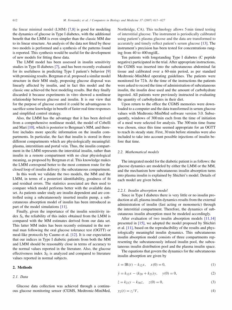
Patients with similar pattern in glucose dynamics have beengrouped together and only one figure for each group is shown inFigs. 1–5 , for the fitted windows. The same applies to nonfittedwindows in Figs. 6–11 . In each figure the first subplot showsthe amount of carbohydrate ingested (right panel) and the rate ofglucose absorption RA (left panel), the second subplot includesthe bolus injection and continuous insulin infusion IR (right)together with the simulated plasma insulin dynamics y2 (left)and finally the third subplot shows the dynamics of plasmaglucose concentration y1. The goodness of fit expressed in termsof the R2 for both the LMM and MM is included in each figurefor the particular patient chosen to represent the group.


0 50 100 150 200 250 3000

100

200

300

400

500

600

RA

(m

g/m

in)

0 50 100 150 200 250 3000

10

20

30

40

50

60

Glu

cose

load

(g

/5 m

in)

0 50 100 150 200 250 3000

50

100

y 2 (µ

U/m

l)

0 50 100 150 200 250 3000

5

10

IR (

U/5

min

)

0 50 100 150 200 250 3000

50

100

150

200

Time (mins)

y 1 (m

g/d

l)

DataLMM, R2= 0.83MM, R2= 0.99

Fig. 2. Group F2. Glucose is controlled within a short period of time (less than 120 min) in Patient 60 (w3) which is shown in this figure. This pattern is alsoobserved in Patient 60 (w2, w5), Patient 65 (w2, w4), and Patient 66 (w1). The high value of the insulin sensitivity index in these patients might explain thisbehavior.

0 50 100 150 200 250 3000

100

200

300

400

500

600

RA

(m

g/m

in)

0 50 100 150 200 250 3000

10

20

30

40

50

60

Glu

cose

load

(g

/5 m

in)

0 50 100 150 200 250 3000

50

100

y 2 (µU

/ml)

y 1 (µU

/ml)

0 50 100 150 200 250 3000

5

10

IR (

U/5

min

)

0 50 100 150 200 250 3000

100

200

300

Time (mins)

DataLMM, R2= 0.94MM, R2= 0.86

Fig. 3. Group F3. Rather slow dynamics compared to Group I and Group II. Slow control might be due to the delay in supplying the insulin input. This figurecorresponds to fitted data from Patient 22 (w1).


0 50 100 150 200 250 3000

500

1000

RA

(m

g/m

in)

0 50 100 150 200 250 3000

50

100

Glu

cose

load

(g/

5 m

in)

0 50 100 150 200 250 3000

1020304050607080

y 2 (µ

U/m

l)

0 50 100 150 200 250 3000246810121416

IR (

U/5

min

)

0 50 100 150 200 250 300100

150

200

250

Time (mins)

y 1 (

mg

/dl)

DataLMM, R2= 0.88MM, R2= 0.9

Fig. 4. Group F4. Biphasic response resulting from a high glucose load in Patient 2 (w3).

0 50 100 150 200 250 3000

100

200

300

400

500

600

RA

(m

g/m

in)

0 50 100 150 200 250 3000

10

20

30

40

50

60

Glu

cose

load

(g/

5 m

in)

0 50 100 200 250 3000

10

20

30

40

50

60

y 2 (µ

U/m

l)

0 50 100 150 200 250 3000

1

2

3

4

5

6

IR (

U/5

min

)

0 50 100 150 200 250 3000

100

200

300

Time (mins)

y 1 (m

g/d

l)

DataLMM, R2= 0.88MM, R2= 0.87

Fig. 5. Group F5. Glucose increases towards a maximum value and only begins to descend during the last 50 min. This pattern is only observed in Patient 6(w1). Two insulin injections are supplied but the first one is applied early and the second one rather late, which might explain why the resulting control isnot adequate.


0 50 100 150 200 250 3000

500

1000

RA

(m

g/m

in)

0 50 100 150 200 250 3000

50

100

Glu

cose

load

(g/

5 m

in)

0 50 100 150 200 250 3000

10

20

30

40

y 2 ( µ

U/m

l)

0 50 100 150 200 250 3000

0.05

0.1

0.15

0.2

IR (

U/5

min

)

0 50 100 150 200 250 30040

60

80

100

120

Time (mins)

y 1 (m

g/dl

)

Data

LMM, R2

MM, R2

Fig. 6. Group NF1. Patients in this group administered only basal or no insulin at all (17 cases). The fit in this figure corresponds to data from Patient 27(w1), in which insulin is only supplied at basal rate.

0 50 100 150 200 250 3000

100

200

300

400

500

600

RA

(m

g/m

in)

0 50 100 150 200 250 3000

5

10

15

20

25

30

Glu

cose

load

(g

/5 m

in)

0 50 100 150 200 250 3000

100

200

y 2 (µ

U/m

l)

0 50 100 150 200 250 3000

5

10

IR (

U/5

min

)

0 50 100 150 200 250 300100

150

200

250

Time (mins)

y 1 (m

g/dl

)

Data

LMM, R2

MM, R2

Fig. 7. Group NF2. Patients received more than two insulin bolus injections (two cases). This figure shows the fit for Patient 22 (w2) who applied multipleinsulin injections.


0 50 100 150 200 250 3000

100

200

300

400

500

600

RA

(m

g/m

in)

0 50 100 150 200 250 3000

10

20

30

40

50

60

Glu

cose

load

(g

/5 m

in)

0 50 100 150 200 250 30020

40

60

y 2 (µ

U/m

l)

0 50 100 150 200 250 3000

5

10

IR (

U/5

min

)

0 50 100 150 200 250 3000

100

200

300

400

Time (mins)

y 1 (m

g/dl

)

Data

LMM, R2= 0.65

MM, R2= 0.64

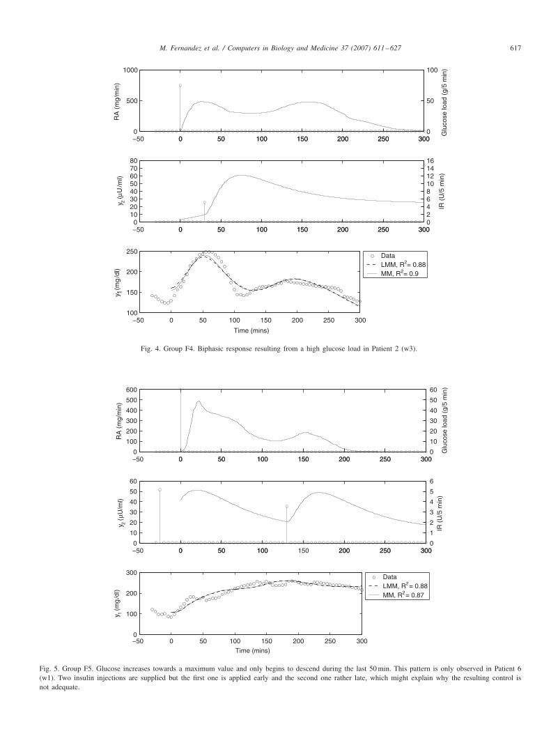
Fig. 8. Group NF3. Patients with a certain degree of insulin resistance and inadequate timing of insulin supply (nine cases). Data from Patient 54 (w1) havebeen plotted and the slow reaction to the initial insulin injection can be appreciated.

0 50 100 150 200 250 3000

100

200

300

400

500

600

RA

(m

g/m

in)

0 50 100 150 200 250 3000

10

20

30

40

50

60

Glu

cose

load

(g/

5 m

in)

0 50 100 150 200 250 3000

50

100

150

y 2 (µU

/ml)

0 50 100 150 200 250 3000

2

4

6

IR (

U/5

min

)

0 50 100 150 200 250 3000

50

100

150

Time (mins)

y 1 (m

g/dl

)

Data

LMM, R2= 0.05

MM, R2

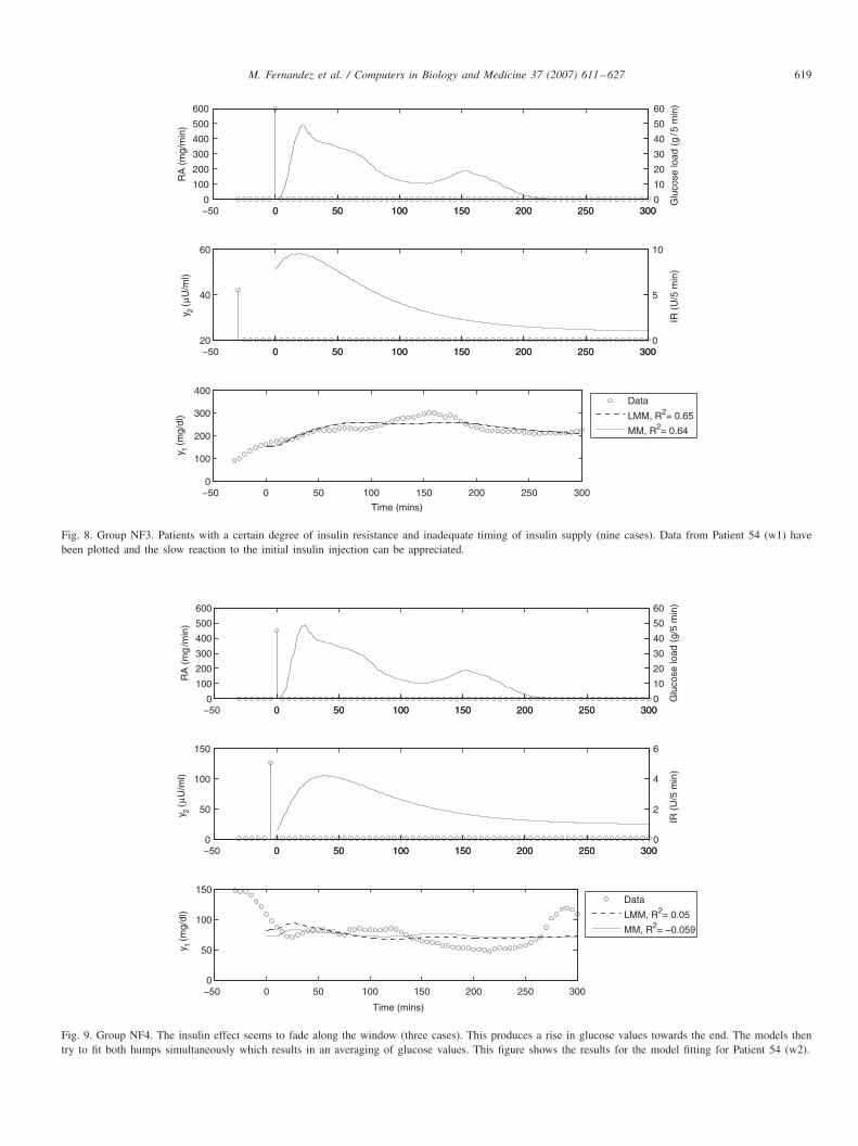
Fig. 9. Group NF4. The insulin effect seems to fade along the window (three cases). This produces a rise in glucose values towards the end. The models thentry to fit both humps simultaneously which results in an averaging of glucose values. This figure shows the results for the model fitting for Patient 54 (w2).


0 50 100 150 200 250 3000

100

200

300

400

500

600

RA

(m

g/m

in)

0 50 100 150 200 250 3000

5

10

15

20

25

30

Glu

cose

load

(g/

5 m

in)

0 50 100 150 200 250 3000

50

100

y 2 ( µ

U/m

l)

0 50 100 150 200 250 3000

5

10

IR (

U/5

min

)

0 50 100 150 200 250 300100

200

300

400

500

Time (mins)

y 1 (m

g/dl

)

Data

LMM, R2

MM, R2

Fig. 10. Group NF5. The range of action of glucose seems to be too wide and the models produced a fit by averaging the glucose values. Data from Patient65 (w1) are plotted.

0 50 100 150 200 250 3000

200

400

600

RA

(m

g/m

in)

0 50 100 150 200 250 3000

5

10

15

Glu

cose

load

(g/

5 m

in)

0 50 100 150 200 250 30030

40

50

y 2 (µ

U/m

l)

0 50 100 150 200 250 3000

5

10

IR (

U/5

min

)

0 50 100 150 200 250 3000

50

100

150

Time (mins)

y 1 (m

g/d

l)

Data

LMM, R2= 0.15

MM, R2= 0.15

Fig. 11. Group NF6. Patients in this group showed an oscillatory pattern that could not be fitted by the models. This figure illustrates these dynamicscorresponding to Patient 2 (w1) data.


Table 3Estimates of the insulin sensitivity index SI and SL

I expressed in the sameunits

Patient Window SLI (1/min per �U/ml) SI (1/min per �U/ml)

66 1 9.38 11.9965 4 9.86 42.05

2 10.09 11.1660 5 11.56 19.13

3 9.15 15.422 6.77 7.75

54 3 3.74 3.6737 3 3.57 2.9327 2 3.53 4.4922 1 16.96 12.39

6 1 6.60 3.062 3 3.20 3.06

2 1.77 2.09

Mean 7.40 10.71Std. 4.30 10.91

3.1.1. Patterns in fitted windowsA group label ranging from F1 to F5 has been chosen to iden-

tify the five different patterns observed in the fitted windows.In Group F1 we can see a pattern close to the normal glucosedynamics during an OGTT. Glucose reaches a maximum valueshortly after glucose load is supplied at t = 0 and graduallydescends towards a steady-state level (see Fig. 1). One or twoconsecutive insulin bolus injections are the common controlstrategy followed by this group of patients, which includes Pa-tient 2 (w2), Patient 27 (w2), Patient 37 (w3), and Patient 54(w3). In Group F2 the same insulin strategy is followed but theinitial increase in glucose is not present or is moderate com-pared to Group F1 dynamics. The main difference with the firstgroup is that glucose moves rather quickly (less than 120 min)to the steady state (see Fig. 2). A possible explanation for thisbehavior is that patients in this group, namely Patient 60 (w2,w3, w5), Patient 65 (w2, w4), and Patient 66 (w1), are moresensitive to insulin than others. This hypothesis seems to beconfirmed by the insulin sensitivity index SI values reported inTable 3 for these patients, where all of them exhibit the highestvalues estimated both with the MM and LMM. Although in thistable Patient 22 (w1) also shows a high SI, insulin is suppliedvery late in this case and therefore the sudden drop in glucosecannot be appreciated from the dynamics plotted. This data setfrom Patient 22 conforms Group F3 which shows a rather slowdynamics compared to Group F1 and Group F2 (see Fig. 3).Glucose reaches a maximum value and slowly moves towardsthe steady state, where the slow control could be explained bythe significant delay (after 80 min) in supplying the insulin in-put. In Group F4 a biphasic response is observed probably as aresult from the high glucose load of 75 g (see Fig. 4). Finally,Group F5 shows a patient in which poor control is achieved(see Fig. 5). Glucose increases gradually towards a maximumvalue and only begins to descend during the last 50 min despiteof two insulin bolus injections. The fact that one injection isapplied early (at −30 min) and the other one is late (at 130 min)could explain the lack of proper control.

3.1.2. Patterns in nonfitted windowsThe nonfitted windows can be grouped into six categories

identified with labels NF1–NF6. The first two groups, namelyGroup NF1 and Group NF2, include those patients that followedan inappropriate insulin therapy. In Group NF1 we includedthose patients that during the specified time frame administeredonly basal insulin or no insulin at all (17 cases) whilst in GroupNF2 those that received more than two bolus insulin injections(2 cases). In Fig. 6, we show the dynamics for the data setcorresponding to Patient 27 (w1) as representative for GroupNF1 which includes 57% of the nonfitted windows. The secondsubplot in this figure shows a constant base feed of insulinat very low levels (0.1 U/5 min), which results in an almostsustained increase in glucose values. In contrast to this case,Fig. 7 shows a patient from Group NF2 who applied multipleinsulin injections, namely Patient 22 (w2). Both Figs. 6 and 7,show a poor fit of the models, with a negative goodness-of-fitmeasure R2. Negative values for R2 occur when the model fitsthe data worse than the horizontal line at the mean value.

The third group identified as Group NF3, includes those win-dows where insulin injections have very little effect, whichindicates that a certain degree of insulin resistance might bepresent. Since data from insulin resistant patients have been fit-ted as reported in the previous section, other factors had to beconsidered as possible sources for the fitting method to fail. Inthis respect, we also observed this group of patients suppliedtheir insulin rather early, late or both, which together with thelow insulin sensitivity might explain why the control achievedwas inadequate and the models were not able to fit the data.

This group (NF3) holds nine cases, which accounts for 27%of the total nonfitted windows. In this set, we placed Patient12 (all five windows), Patient 6 (w2,w5), Patient 54 (w1) andPatient 37 (w4). From Table 3, we can see that Patient 54 andPatient 37 have rather low values for the sensitivity index SIwhilst Patient 6 index is slightly below the mean value. Thisseems to confirm the hypothesis of insulin resistance in thesepatients. Note that this index is not shown in this table forPatient 12 since no window out of five for this patient wasdeemed fit, but it was consistently one order of magnitude belowthe reported values (SI was less than 1) with only one windowwith and index value slightly higher (SI =3). One example of acharacteristic patient in this group is shown in Fig. 8 where datafrom Patient 54 (w1) have been plotted and the slow reactionto the initial insulin injection can be appreciated.

The fourth group or Group NF4 contains windows where theinsulin effect seems to fade along the window. This producesa rise in glucose values towards the end. The glucose valuesfor windows in this group look like two ‘humps’ separated bya valley. The models then try to fit both humps simultaneouslywhich results in an averaging of glucose values. The reasonwhy insulin is not effective any more at the end could not befound from the available data in this study. Fig. 9 shows theresults for the model fitting for Patient 54 (w2). This groupcontains only three cases which represents 9% of all nonfittedwindows.

The pattern found in Group NF5 is illustrated in Fig. 10 andincludes data from Patient 65 (w1) only. The slow increase with


no control in the glucose dynamics observed in this windowcannot be explained by the absence of insulin supply or lowsensitivity to insulin, since this patient supplied a bolus injec-tion and showed high values for SI in the windows that couldbe fitted. A slow absorption of the ingested glucose could bepossible, but could not be explained from the available data inthis study. This resulted in dynamics close to a line which in-creases monotonically. The range of action of glucose seemsto be too wide and the models produced a fit by averaging theglucose values.

Group NF6 includes Patient 2 (w1, w4) showing an oscil-latory pattern that could not be fitted by the models. Fig. 11illustrates these dynamics corresponding to Patient 2 (w1) data.We could not find a reasonable explanation for such behaviorfrom the data available in this study.

3.1.3. Analysis of resultsFrom the set of accepted windows, some properties seem to

be common among them:

• Only one or two insulin bolus injections can be included forthe models to fit the dynamics of glucose. When three ormore injections were supplied none of the MMs were ableto account for such complex dynamics. Thus, both modelsare able to follow a single or biphasic insulin response, suchas the one exhibited by the natural pancreas.

• At least an insulin bolus injection should be administered.When no bolus injection was present both models failed tofit the dynamics of glucose. This could be explained by thefact that they were formulated and identified to describe theinteraction between insulin and glucose after a glucose stim-ulus, when there is an immediate response from the pancreasto achieve normoglycemia.

• The range of action of glucose dynamics does not seem to betoo wide in all accepted windows, meaning that the patient iscontrolled reasonably well. When for some reason the insulindid not seem to work well for the patient, the dynamics ofglucose showed large variations and both models failed to fitthese data. This situation might be as a consequence of thepatient choosing a bolus injection that is not the right choicefor the amount of carbohydrate ingested.

The number of fitted windows can be said to be very smallwhen compared to the total available windows. Would the MM,either the linear or classic version, therefore be the right choicefor a closed-loop system since it is not able to describe severalprofiles of the patients under study? It is clear that none of theMMs are able to follow complex situations such as the presenceof several bolus injections, the absence of insulin supply, orinadequate insulin dosage, but all these are common situationswhen glucose is controlled in an open-loop fashion, and willhopefully not be present when closing the loop of control.

3.2. Initial estimates

It is interesting to note that the initial estimate for SLI =2.1962

(g/min per U) we have obtained for the LMM in Table 1 is

related to the IVGTT value SLI = 0.8121 (g/min per U) of

the LMM reported in [7] as follows: the value of SLI from

the OGTT is about twice the IVGTT estimate, as in the workpublished by Caumo and coworkers for the average SI in 10patients.

In their study, Caumo et al. compared the mean SI value de-rived from the MM after an OGTT with the mean SI duringthe IVGTT and although these indices correlated well, the ab-solute value for the OGTT was nearly twice the value obtainedfor the IVGTT.

However, our estimates are the result of a single simulation inthe normal man and further experiments including more patientsshould be performed in order to see if this relationship stillholds.

Also, for the initial estimates of the LMM parameter SLG

in both experiments, it results that SLG = 0.0182 (1/min) from

the OGTT in Table 1 is about half its corresponding valueSL

G = 0.0325 (1/min) for an IVGTT [7]. Caumo et al. did notestimate the average value of this parameter, but took it fromthe literature and can also be concluded that when the literaturevalue SG = 0.024 (dL/kg min) is multiplied by the mean V1 =1.4 (dL/kg) they obtained in their experiments, the resultingSG = 0.0171 (1/min) is also about half the IVGTT value forSG = 0.0300 (1/min) for the classic MM [19].

This coincidence emphasizes that even for a LMM the unex-pected result obtained by Caumo et al. for which the SI indexestimated from the OGTT is numerically twice as great as SIfrom the IVGTT could also be true. Also, that index SG ob-tained from the OGTT could be half the value obtained fromthe IVGTT.

3.3. Metabolic indices

In Tables 4 and 5 parameter estimates of the MM and LMM,respectively, are reported. Comparing the MM and LMM glu-cose effectiveness index reported in both tables, we found themean value for SL

G = 0.0407 ± 0.0459 (1/min) is significantlydifferent from SG = 0.0266 ± 0.0319 (1/min) according to theWilcoxon signed rank test (p-value=2.4414×10−4, �=0.001),but Spearman’s rank correlation coefficient shows they cor-relate very well (Rs = 0.91, p-value = 0.0015, � = 0.01) asshown in Fig. 12, where the regression line is also included(Slope = 0.67 ± 0.04, p-value = 2.75 × 10−9, � = 0.001; Inter-cept: −0.0018 ± 0.0023).

The literature value for this index has been reported to beSG = 0.0171 (1/min) [12] (see Section 3.2 for details). Thus,according to our results it could be that both the MM andLMM are overestimating this value. Further analysis should beperformed to conclude on this observation.

Concerning the insulin sensitivity index, Table 3 includes theestimates of the insulin sensitivity index in the same units forboth models. It can be appreciated that the mean value of thisparameter is SL

I = 7.40 for the LMM and SI = 10.71 for theMM both in (1/min per �U/ml). According to the Wilcoxonsigned rank test these two indices are not significantly different(p-value = 0.1909, � = 0.001) and there is a strong correlationbetween them as demonstrated by Spearman’s test (Rs = 0.83,


Table 4MM optimal parameter estimates

Patient Window SG SI p2 y10

(1/min) (10−4 × 1/ min per �U/ml) (1/min) (mg/dL)

2 2 0.0089 2.0933 0.0143 142.83 0.0012 3.0611 0.0734 155.3

6 1 0.0053 3.0567 0.0122 106.922 1 0.0240 12.3907 0.0030 218.627 2 0.0058 4.4885 0.0085 168.837 3 0.0165 2.9326 0.0030 329.954 3 0.0569 3.6650 0.0125 97.460 2 0.0080 7.7475 0.3000 106.1

3 0.0226 15.4176 0.1644 149.75 0.1200 19.1266 0.1176 138.7

65 2 0.0319 11.1547 0.3000 188.34 0.0322 42.0456 0.0030 363.1

66 1 0.0125 11.9898 0.0484 360.4

Mean 0.0266 10.7053 0.0816 194.3Std. 0.0319 10.9107 0.1091 95.7

Table 5LMM optimal parameter estimates

Patient Window SLG SL

I pL2 q10

(1/min) (g/U min) (1/min) (g)

2 2 0.0132 0.6481 0.0223 27.373 0.0070 1.2862 0.1097 30.11

6 1 0.0055 1.7985 0.0135 19.6222 1 0.0426 9.8290 0.0020 29.7227 2 0.0145 1.5215 0.0115 33.5137 3 0.0226 2.9670 0.0024 61.7254 3 0.0614 0.9171 0.0142 15.7160 2 0.0257 1.5723 0.2000 11.15

3 0.0480 2.6807 0.2000 14.065 0.1820 3.4735 0.0596 14.42

65 2 0.0481 4.5736 0.2000 28.684 0.0373 8.6569 0.0097 55.54

66 1 0.0211 8.5015 0.0922 46.13

Mean 0.0407 3.7251 0.0721 29.83Std. 0.0459 3.2061 0.0804 16.08

p-value = 0.0040, �= 0.01) and the regression line included inFig. 12 (Slope=1.59±0.35, p-value=8.33×10−4, �=0.001;Intercept: −2.28 ± 2.97). These tests confirm that accuracy ismaintained when this index is estimated by either model.

From Caumo et al. [12] we find that SI = 9.71 (1/min per�U/ml) as a result of the product between the mean SI =13.6×10−4 (dL/kg min per �U/ml) and the mean V1 = 1.4 (dL/kg).This number is very close in absolute value to the index we haveobtained for the MM (9.71 vs. 10.71). Estimates of SL

I seem tobe slightly underestimated with respect to the index reported byCaumo et al. (7.40 vs. 9.71). But if underestimation is certainlyoccurring this needs to be addressed in future studies.

One possible source of error though could be the nor-malization performed to make SL

I comparable to SI sincethe volume of distribution V used in the normalization isonly an approximation to the plasma insulin distributionvolume.

Finally, although p2 is not considered a metabolic index itis interesting to note that it is not significantly different inboth models (p-value = 0.6848, � = 0.001) and it also corre-lates well as shown in Fig. 12 (Rs = 0.97, p-value = 7.81 ×10−4, �=0.001) where the regression line is also included foranalysis (Slope = 1.28 ± 0.18, p-value = 1.56 × 10−5, � =0.001; Intercept: −0.0085 ± 0.0187).

3.4. Model validation

In Tables 6 and 7 precision of the MM and LMM is, respec-tively, reported for all accepted windows, whilst the goodness offit is shown in Figs. 1–5. Precision of parameter SG in the MMis unsatisfactory in one of the subjects (CV > 100%) but thisdata set was kept to avoid reducing the set under study even fur-ther. This decision was made in the light that the CV value wasnot very high (CV=118%) and that it was good for the LMM.


0 5 10 15 200

10

20

30

40

50

SIL (10 ×1/min per µU/ml)

SI (

10×1

/min

per

µU

/ml)

Rs = 0.83, R2 = 0.88, SI I

L

0 0.05 0.1 0.15 0.20

0.02

0.04

0.06

0.08

0.1

0.12

SGL (1/min)

SG

(1/

min

)

Rs = 0.91, R2 = 0.98, SG G

L

0 0.05 0.1 0.15 0.20

0.05

0.1

0.15

0.2

0.25

p2L (1/min)

p 2 (1/

min

)

Rs = 0.97, R = 0.86, p2 2

L

Fig. 12. Scatter plots and regression lines between the metabolic indices from the MM and LMM, including the R2 value resulting from the fit. The Spearmantest values are also reported.

Table 6MM parameter precision expressed in terms of the coefficient of variation (CV)

Patient Window CV(SG) CV(SI) CV(p2) CV(y10)

2 2 64.70 28.84 58.08 1.943 118.76 1.39 9.75 1.08

6 1 7.44 15.79 22.89 1.9222 1 10.49 68.17 75.76 2.0727 2 60.14 45.69 68.77 0.8037 3 18.79 65.00 77.35 0.8954 3 8.97 13.51 24.61 1.2560 2 10.22 2.29 35.17 2.54

3 2.73 1.66 5.91 0.535 17.93 16.22 28.04 1.20

65 2 5.98 3.49 58.54 1.354 10.12 29.99 28.43 1.01

66 1 3.14 1.90 5.34 0.34

Mean 26.11 22.61 38.36 1.30Std. 34.43 23.74 26.21 0.65

Overall, the precision of the LMM is better than the MMwith systematic lower mean values for CVs in all characteristicmodel parameters (initial conditions are excluded). These CVsare as follows for the LMM and MM, respectively: 12% vs.26% in SG, 14% vs. 23% in SI, 29% vs. 38% in p2.

The average residuals are shown in Fig. 13 for both modelsshowing deviations that have a pattern. Furthermore, the Runstest confirmed residuals derived from the LMM and MM fittingwere not random for any of the windows under study.

The fact that residuals are not random could be due to anyof these three different sources:

1. The MM itself is not able to follow the dynamics of Type Idiabetic patients.

2. Measurement errors may contain systematic errors. In thiscase structured noise should be removed from the glucosesignal. The use of model-based signal enhancement couldbe useful for this purpose [9].


Table 7LMM parameter precision expressed in terms of the coefficient of variation CV

Patient Window CV(SLG) CV(SL

I ) CV(pL2 ) CV(q10)

2 2 34.38 12.15 39.05 1.743 27.21 1.54 22.91 1.10

6 1 6.91 14.77 20.27 1.8822 1 8.41 39.69 39.82 1.4527 2 14.98 13.02 21.45 0.9537 3 12.42 55.55 62.46 0.8654 3 7.36 11.28 19.79 1.1960 2 6.12 2.46 33.17 2.99

3 8.37 3.43 32.59 2.225 14.37 14.91 13.94 1.32

65 2 5.07 4.05 49.18 1.334 9.65 12.76 9.81 1.05

66 1 1.72 1.07 6.78 0.43

Mean 12.08 14.36 28.55 1.42Std. 9.19 15.98 16.11 0.66

0 50 100 150 200 250 300

0

2

4

6

8

10

Time (mins)

Res

idua

ls (

unitl

ess)

LMMMM

Fig. 13. Mean residuals are an average of the residuals obtained when fitting the MM and LMM in all accepted windows. They show deviations that have apattern. The Runs test also confirmed residuals were not random for any of the windows under study.

3. The chosen input models are not the right choice for the dataunder study. In this respect, there could be shortcomings ineither of the following:

• The rate of glucose absorption model is oversimplified.For glucose loads different from 45 or 89 g we took asvalid the curve that corresponds to the load closest in valueto these (e.g. if the actual glucose load was 15 g, the curveobtained for 45 g was chosen as the rate of appearance).This approximation will introduce unavoidable errors intothe model until more data can be gathered and betterestimates obtained.

• The insulin absorption model is too simple. A recent pub-lication shows a model like Shichiri’s model underesti-

mates the post meal peak of plasma insulin, whilst im-provement in the model fit was improved when two ab-sorption channels were considered [22].

Further work should consider making these proposed im-provements and the impact on the residuals assessed.

4. Conclusions

From the analysis of the fitted windows it can be concludedthat both the MM and the LMM are able to fit or fail to fit thesame set of windows per patient, showing the same ability todescribe the dynamics of the controlled diabetic patients. The


quality of the fit is the same for both models as the R2 testindicates.

The fact that only a small group of windows was success-fully fitted by both models, could be explained by the complexdynamics that arise in an open-loop controlled diabetic patient,such as the presence of several insulin bolus injections, the ab-sence of insulin supply or inadequate insulin dosage. When oneor more of these situations were present data could not be fittedby either model. However, both models seemed to cope rea-sonably well for a variety of insulin doses and glucose loads.

Overall, the precision of the LMM is better than the MMwith systematic lower mean values for CVs in all characteristicmodel parameters. These CVs are as follows for the LMM andMM, respectively: 12% vs. 26% in SG, 14% vs. 23% in SI,29% vs. 38% in p2.

In terms of accuracy, it can be concluded that the insulinsensitivity index SI can be estimated by either the LMM or theMM with the same accuracy, whilst the glucose effectivenessindex SG is different in both models. Further work is requiredto assess the significance of these differences.

Given all the above mentioned results, the LMM might beof interest for the closed-loop control of diabetic patients be-cause of its simplicity, precision and accuracy of the metabolicindexes.

Finally, the fact that residuals show a systematic patternshould be further studied. Whether this is a result of structurednoise or due to the integrated model’s inability to describe thedata under study remains to be established.

5. Summary

The rationale of the present study is to show that the classicminimal model (MM) proposed by Bergman et al. [6] and aneven simpler version, the linear minimal model (LMM) pre-sented by Fernandez and Atherton [8], are good for modelingthe dynamics of glucose in Type I diabetes. As patient’s understudy are insulin dependent and are controlled using a subcu-taneously inserted insulin pump, the insulin absorption modelproposed by Shichiri et al. [11] has been included. Data setswere collected from 10 patients using the CGMS continuoussensor (Medtronic-Minimed) during 3 days. Subsequently, win-dows of 300 min each from the time of initiation of a meal wereselected for analysis. After fitting of these data, it can be con-cluded that both the MM and the LMM are able to fit or failto fit the same set of windows per patient, showing the sameability for describing the dynamics of the controlled diabeticpatients. However, precision of the LMM is better than the MMwith systematic lower mean values for the coefficient of vari-ation (CV) in all characteristic model parameters. The insulinsensitivity index SL

I derived from the LMM is not significantlydifferent from SI estimated from the MM (�=0.001) and thereis a strong correlation between them (Rs = 0.83, � = 0.01),which confirms that accuracy is maintained when this index isestimated by either model. The mean values are SL

I = 7.40 andSI = 10.71 both in (1/min per �/ml), whilst the literature indexhas been reported to be 9.71 (1/min per �U/ml) in Caumo etal. [12]. On the other hand, glucose effectiveness shows to be

significantly different in both models (� = 0.001) but it cor-relates very well (Rs = 0.91, � = 0.01). The mean values areSL

G = 0.0407 (1/min) and SG = 0.0266 (1/min) for the LMMand MM, respectively, whilst the literature value reported inCaumo et al. [12] is SG = 0.0171 (1/min). Thus, if accuracy ofthis parameter is achieved by the LMM remains to be estab-lished. Given all the above-mentioned results, the LMM mightbe of interest for the closed-loop control of diabetic patients be-cause of its simplicity, precision and accuracy of the metabolicindexes. Finally, the average residuals show systematic devia-tions, meaning that either the measurement errors contain sys-tematic errors or that the integrated model of the patient is notthe right choice for the data under study. Further work shouldbe performed and the impact on residuals assessed.

References

[1] American Diabetes Association. Standards of medical care for patientswith diabetes mellitus (Position Statement), Diabetes Care 21 (Suppl. 1)(1998) S23–S31.

[2] R.S. Parker, F.J. Doyle III, J.E. Harting, N.A. Peppas, Model predictivecontrol for infusion pump insulin delivery, 18th Annual InternationalConference of the IEEE Engineering in Medicine and Biology Society,vol. 5, IEEE, Piscataway, NJ, USA, 1996, pp. 1822–1823.

[3] A. Sano, Adaptive and optimal schemes for control of blood glucoselevels, Biomed. Meas. Inf. Control 1 (1) (1986) 16–22.

[4] Z. Trajanoski, P. Wach, Neural predictive controller for insulin deliveryusing the subcutaneous route, IEEE Trans. Biomed. Eng. 45 (9) (1998)1122–1134.

[5] E.R. Carson, C. Cobelli, L. Finkelstein, The Mathematical Modeling ofMetabolic and Endocrine Systems, Wiley, New York, 1983.

[6] R.N. Bergman, Y.Z. Ider, C.R. Bowden, C. Cobelli, Quantitativeestimation of insulin sensitivity, Am. J. Physiol. 236 (6) (1979)E667–E677.

[7] M. Fernandez-Chas, Insulin sensitivity estimates from a linear modelof glucose disappearance, Ph.D. Thesis, University of Sussex, Brighton,UK, 2001 (British Library Catalogue Number: DXN041838).

[8] M. Fernandez, D.P. Atherton, Analysis of insulin sensitivity estimatesfrom linear models of glucose disappearance, Appl. Math. Comput. 167(1) (2005) 528–538.

[9] M. Fernandez, D. Acosta, M. Villasana, D. Streja, Enhancing parameterprecision and the minimal modeling approach in type I diabetes, in:Proceedings of the 26th Annual International Conference of the IEEEEngineering in Medicine and Biology Society, IEEE Press, New York,2004, pp. 797–800.

[10] C. Cobelli, A. Mari, Validation of mathematical models of complexendocrine-metabolic systems. A case study on a model of glucoseregulation, Med. Biol. Eng. Comput. 21 (1983) 390–399.

[11] M. Shichiri, M. Sakakida, K. Nishida, S. Shimoda, Enhanced, simplifiedglucose sensors: long-term clinical application of wearable artificialpancreas, Artif. Organs 22 (1) (1998) 32–42.

[12] A. Caumo, R.N. Bergman, C. Cobelli, Insulin sensitivity studies frommeal tolerance tests in normal subjects: a minimal model index, J. Clin.Endocrinol. Metab. 85 (11) (2000) 4396–4402.

[13] K. Rebrin, G.M. Steil, Can interstitial glucose assessment replace bloodglucose measurements?, Diabetes Technol. Ther. 2 (3) (2000) 461–472.

[14] Z. Trajanoski, P. Wach, P. Kotanko, A. Ott, F. Skrabal, Phamacokineticmodel for the absorption of subcutaneously injected soluble insulin andmonomeric insulin analogues, Biomed. Tech. 38 (1993) 224–231.

[15] R. Bellazzi, G. Nucci, C. Cobelli, The subcutaneous route to insulindependent diabetes therapy, IEEE Eng. Med. Biol. Mag. 20 (1) (2001)54–64.

[16] M. Fernandez, D.P. Atherton, Linearisation and simplification of anonlinear model of the glucose regulatory system, Diabetes Nutr. Metab.11 (1) (1998) 86 (Abstracts, Symposium on Computers in Diabetes 98).


[17] J. Radziuk, T.J. McDonald, D. Rubentein, J. Dupre, Initial splanchnicextraction of ingested glucose in normal man, Metabolism 27 (6) (1978)657–669.

[18] C. Cobelli, A. Ruggeri, Evaluation of portal/peripheral route and ofalgorithms for insulin delivery in the closed-loop control of glucose indiabetes. A modeling study, IEEE Trans. Biomed. Eng. BME-30 (2)(1983) 93–103.

[19] C. Cobelli, P. Vicini, G. Toffolo, A. Caumo, The hot IVGTT minimalmodels: simultaneous assessment of disposal indices and hepatic glucoserelease, in: J. Lovejoy, R.N. Bergman (Eds.), The Minimal ModelApproach and Determinants of Glucose Tolerance, vol. 262, LouisianaState University Press, Baton Rouge, USA, 1997, pp. E968–E975.

[20] R. Randles, D. Wolfe, Introduction to the Theory of NonparametricStatistics, Wiley, New York, 1979.

[21] A. Wald, J. Wolfowitz, On a test whether two samples are from thesame population, Ann. Math. Statist. 11 (1940) 147–162.

[22] M.E. Willinska, L.J. Chassin, H.C. Schaller, L. Schaupp, T.R. Pieber,R. Hovorka, Insulin kinetics in Type-1 diabetes: continuous and bolusdelivery of rapid acting insulin, IEEE Trans. Biomed. Eng. 52 (1) (2005)3–12.

Margarita Fernandez was born in Venezuela in 1968. She received theB.Sc. degree in Computer Engineering from the Simon Bolivar University,Caracas, Venezuela, in 1992. She began Ph.D. research in Biomedical Engi-neering at the University of Sussex, Brighton, UK, in January 1997, under the

supervision of Prof. D.P. Atherton and finished in January 2001. She has beenan Assistant Professor at Simon Bolivar University since September 2002.From September to December 2005, she was a Visiting Research Fellowin the School of Science of Technology at the University of Sussex. Herresearch interests include mathematical modeling of physiological systems,drug delivery systems and diagnostic indices.

Minaya Villasana received the B.S. degree in applied mathematics fromSimon Bolivar University, Caracas, Venezuela, in 1996 and the M.S. and Ph.D.degrees in Mathematics from Claremont Graduate University, Claremont, CA,in 1999 and 2001, respectively. In the year 2001, she joined the ScientificComputation and Statistic Department, Simon Bolivar University as a seniorlecturer. Her research interests are in the fields of mathematical modelingwith special emphasis for applications in Biology and Medicine.

Dan Streja has received his M.D. degree from IMF (Institute of Medicineand Pharmacy) Bucharest Romania. He is Clinical Professor, Sections ofEndocrinology and Cardiology, Department of Medicine at David GeffenSchool of Medicine at UCLA in Los Angeles, California. He works atthe Grater Los Angeles Veteran Healthcare System in West Los AngelesMedical Center. He also practices as a consultant in endocrinology in amultisubspecialty internal medicine group. He has authored 43 articles, co-authored three medical textbooks and is a reviewer for Journal of GeneralInternal Medicine, Diabetes Care, American Journal of Medicine, Archives ofInternal Medicine and Journal of Clinical Pathology. Dr. Streja has lecturednationally and internationally and has been a member of numerous speakerbureaus.

Documents

Glucose dynamics in Type I diabetes: Insights from the classic and linear minimal models