Embed Size (px)
Citation preview
CH103Physical Chemistry: Introduction to Bonding
G. Naresh Patwari
Room No. 215; Department of Chemistry
2576 7182 [email protected]

Physical Chemistry –I.N. LevinePhysical Chemistry – P.W. AtkinsPhysical Chemistry: A Molecular Approach – McQuarrie and Simon
Websites:http://www.chem.iitb.ac.in/~naresh/courses.html
www.chem.iitb.ac.in/academics/menu.php
IITB-Moodle http://moodle.iitb.ac.in
http://ocw.mit.edu/OcwWeb/web/courses/courses/index.htm#Chemistry
http://education.jimmyr.com/Berkeley_Chemistry_Courses_23_2008.php
Recommended Texts (Physical Chemistry)

What Do You Get to LEARN?
�Why Chemistry?
� Classical Mechanics Doesn't Work all the time!
� Is there an alternative? QUANTUM MECHANICS
�Origin of Quantization & Schrodinger Equation
� Applications of Quantum Mechanics to Chemistry
� Atomic Structure; Chemical Bonding; Molecular Structure
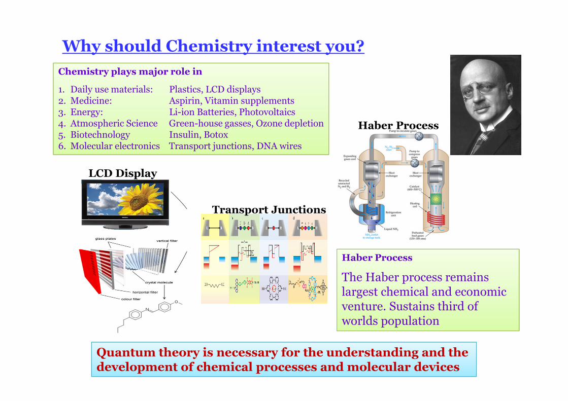
Why should Chemistry interest you?
Chemistry plays major role in
1. Daily use materials: Plastics, LCD displays2. Medicine: Aspirin, Vitamin supplements3. Energy: Li-ion Batteries, Photovoltaics4. Atmospheric Science Green-house gasses, Ozone depletion 5. Biotechnology Insulin, Botox6. Molecular electronics Transport junctions, DNA wires
Haber Process
Haber Process
The Haber process remains largest chemical and economic venture. Sustains third of worlds population
Transport Junctions
Quantum theory is necessary for the understanding and the development of chemical processes and molecular devices
LCD Display
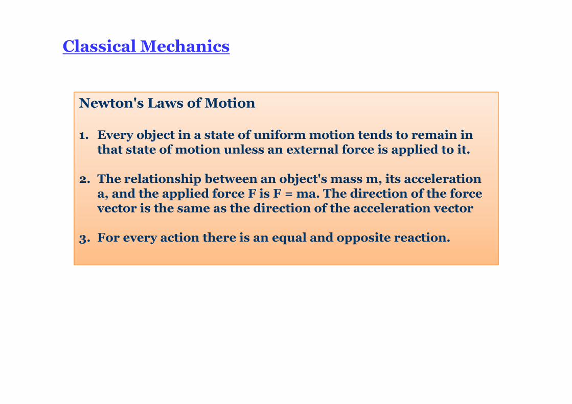
Classical Mechanics
Newton's Laws of Motion
1. Every object in a state of uniform motion tends to remain in that state of motion unless an external force is applied to it.
2. The relationship between an object's mass m, its acceleration a, and the applied force F is F = ma. The direction of the force vector is the same as the direction of the acceleration vector
3. For every action there is an equal and opposite reaction.
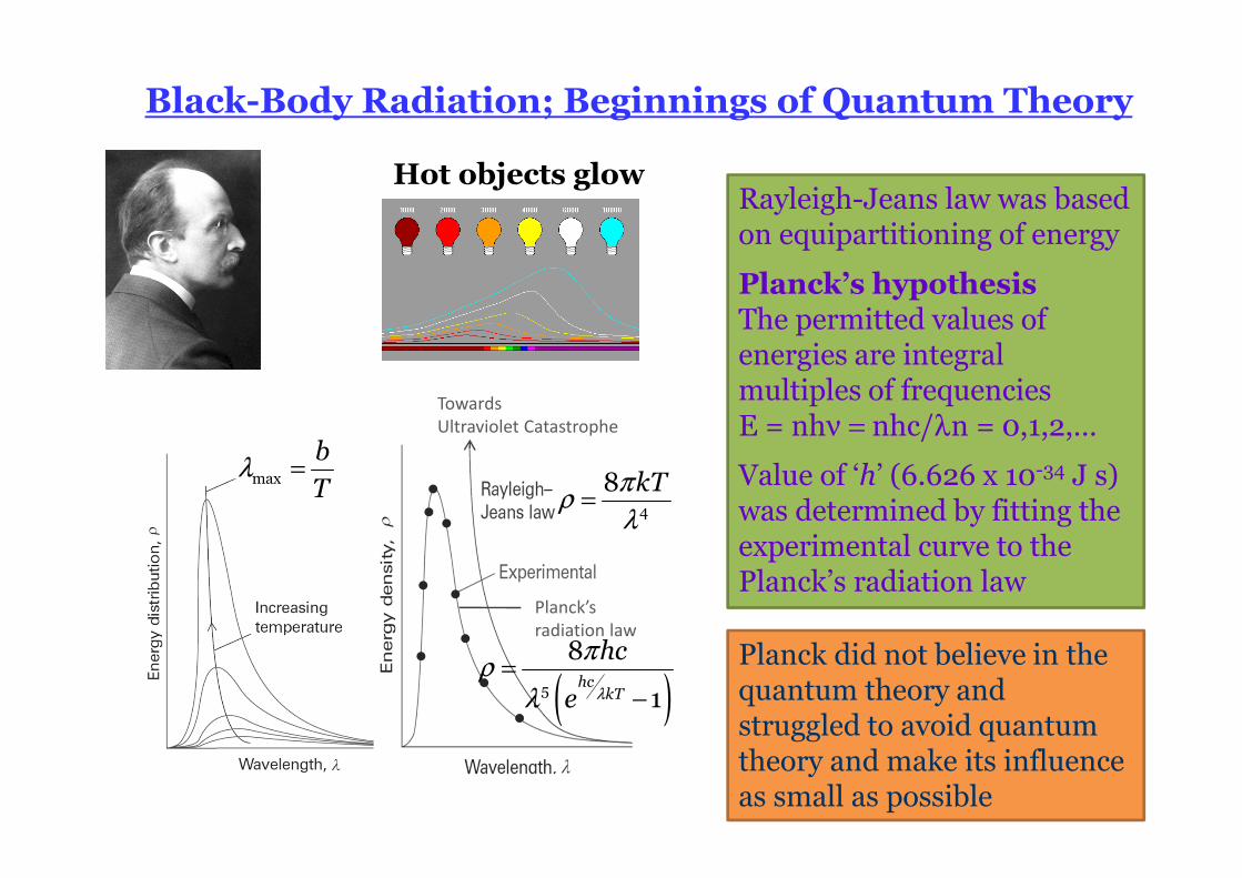
Black-Body Radiation; Beginnings of Quantum Theory
Rayleigh-Jeans law was based on equipartitioning of energy
Planck’s hypothesisThe permitted values of energies are integral multiples of frequenciesE = nhν = nhc/λn = 0,1,2,…
Value of ‘h’ (6.626 x 10⁻³⁴ J s) was determined by fitting the experimental curve to the Planck’s radiation law
kT4
8πρ
λ=
Planck’s
radiation law
( )hckT
hc
e5
8
1λ
πρ
λ=
−
Towards
Ultraviolet Catastrophe
Hot objects glow
Planck did not believe in the quantum theory and struggled to avoid quantum theory and make its influence as small as possible
λ =bTmax
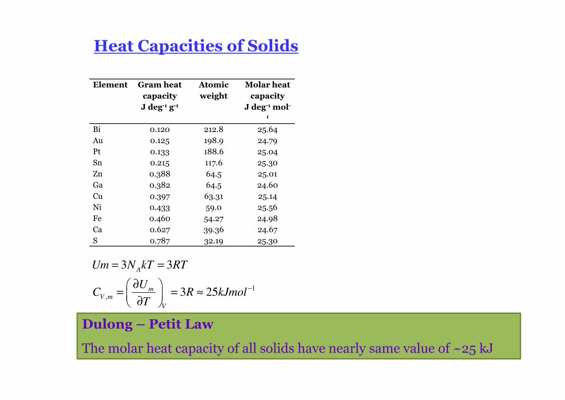
Heat Capacities of Solids
Dulong – Petit Law
The molar heat capacity of all solids have nearly same value of ~25 kJ
Element Gram heat
capacity
J deg-1 g-1
Atomic
weight
Molar heat
capacity
J deg-1mol-
1
Bi 0.120 212.8 25.64Au 0.125 198.9 24.79Pt 0.133 188.6 25.04Sn 0.215 117.6 25.30Zn 0.388 64.5 25.01Ga 0.382 64.5 24.60Cu 0.397 63.31 25.14Ni 0.433 59.0 25.56Fe 0.460 54.27 24.98Ca 0.627 39.36 24.67S 0.787 32.19 25.30
1
,
3 3
3 25
A
mV m
V
Um N kT RT
UC R kJmol
T
−
= =
∂ = = ≈
∂
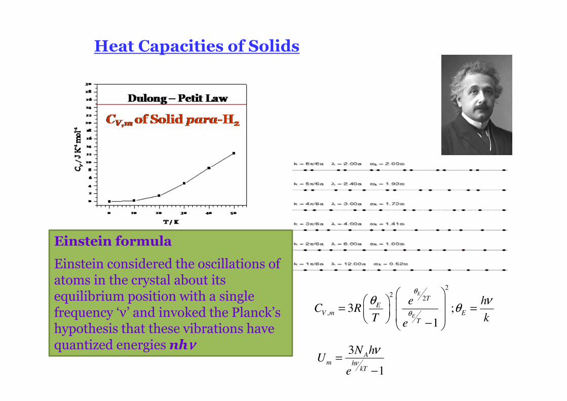
Heat Capacities of Solids
Einstein formula
Einstein considered the oscillations of atoms in the crystal about its equilibrium position with a single frequency ‘ν’ and invoked the Planck’s hypothesis that these vibrations have quantized energies nhνννν
22
2
, 3 ;
1
E
E
TE
V m E
T
e hC R
T ke
θ
θ
θ νθ
= = −
3
1
Am h
kT
N hU
eν
ν=
−
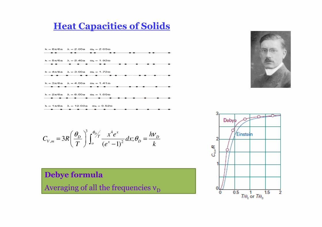
Heat Capacities of Solids
Debye formula
Averaging of all the frequencies νD
3 4
, 23 ;
( 1)
D xTD D
V m Dxo
hx eC R dx
T e k
θθ νθ
= =
− ∫
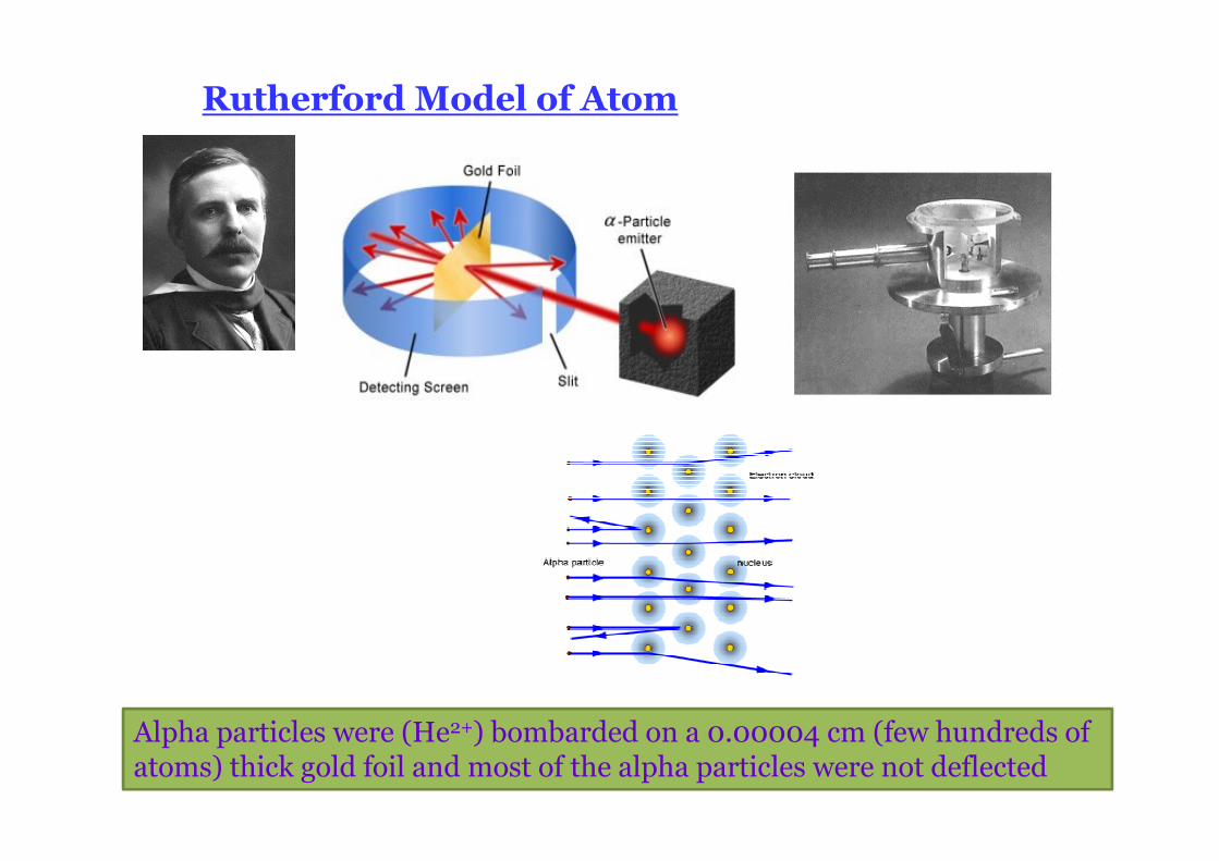
Rutherford Model of Atom
Alpha particles were (He2+) bombarded on a 0.00004 cm (few hundreds of atoms) thick gold foil and most of the alpha particles were not deflected
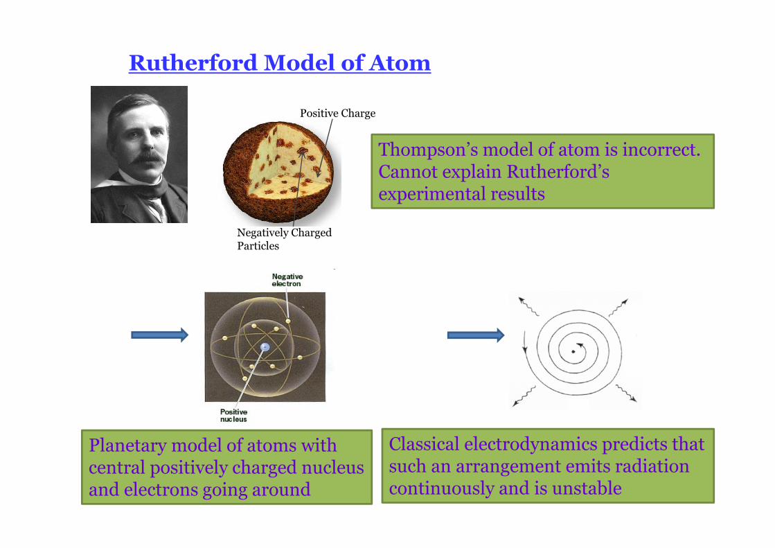
Rutherford Model of Atom
Positive Charge
Negatively ChargedParticles
Thompson’s model of atom is incorrect. Cannot explain Rutherford’s experimental results
Planetary model of atoms with central positively charged nucleus and electrons going around
Classical electrodynamics predicts that such an arrangement emits radiation continuously and is unstable
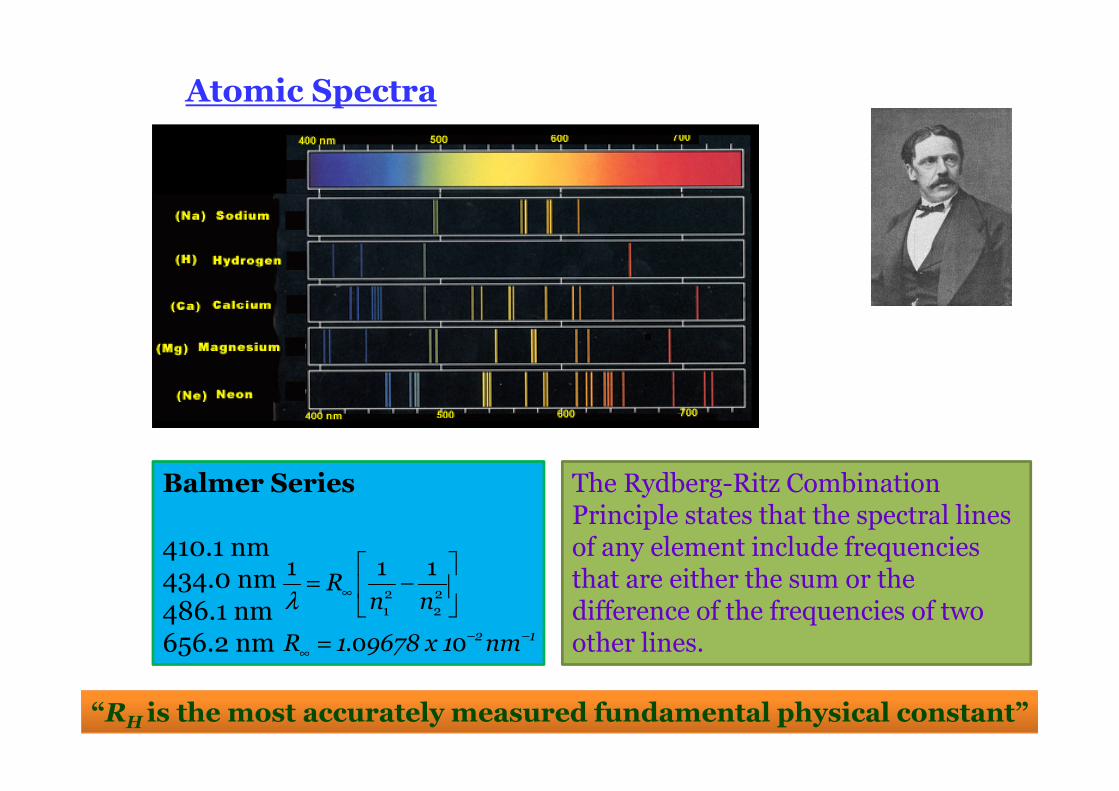
Atomic Spectra
Balmer Series
410.1 nm434.0 nm486.1 nm656.2 nm 2 1
Rn n
R 1 9678 x 1 nm
2 21 2
1 1 1
.0 0
λ ∞
− −
∞
= −
=
“RH is the most accurately measured fundamental physical constant”
The Rydberg-Ritz Combination Principle states that the spectral lines of any element include frequencies that are either the sum or the difference of the frequencies of two other lines.
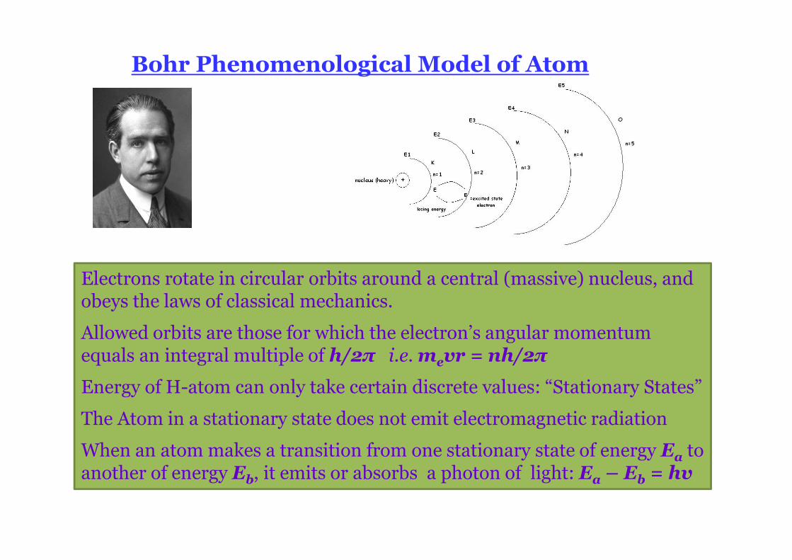
Bohr Phenomenological Model of Atom
Electrons rotate in circular orbits around a central (massive) nucleus, and obeys the laws of classical mechanics.
Allowed orbits are those for which the electron’s angular momentum equals an integral multiple of h/2π i.e.mevr = nh/2π
Energy of H-atom can only take certain discrete values: “Stationary States”
The Atom in a stationary state does not emit electromagnetic radiation
When an atom makes a transition from one stationary state of energy Ea to another of energy Eb, it emits or absorbs a photon of light: Ea – Eb = hv
Energy expression
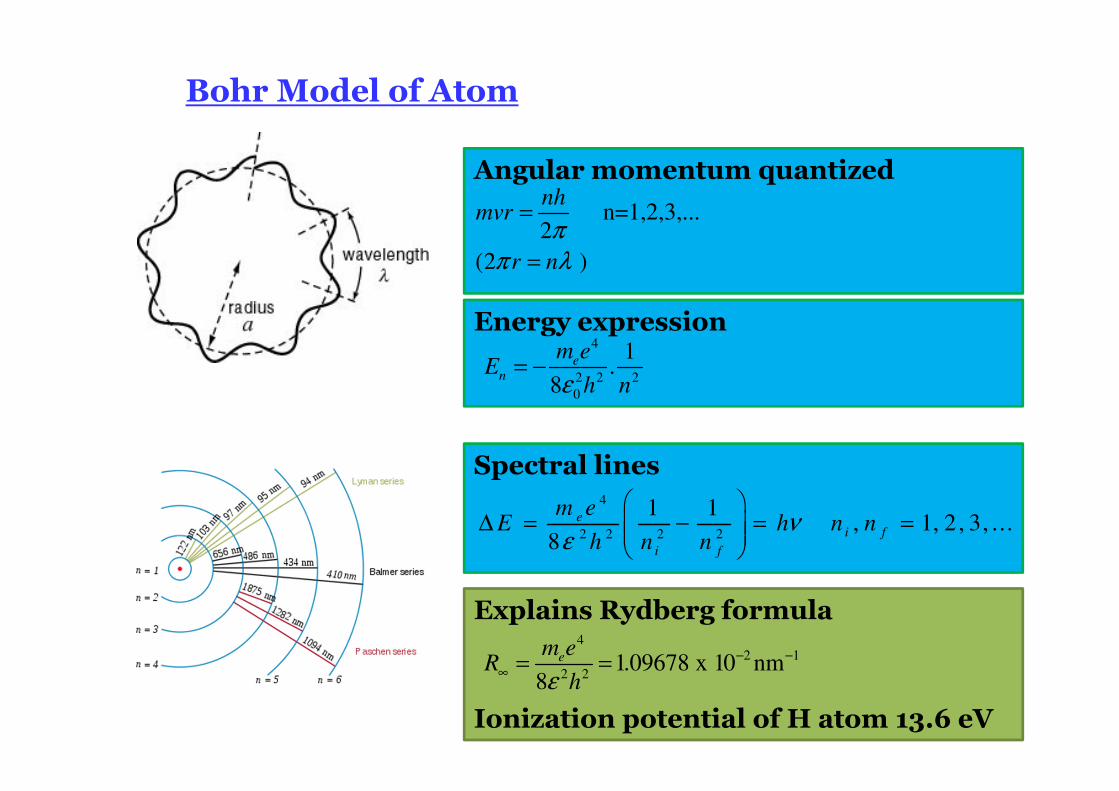
Bohr Model of Atom
Angular momentum quantized
n=1,2,3,...2
(2 )
ππ λ
=
=
nhmvr
r n
4
2 2 2
0
1.
8ε= − e
n
m eE
h n
Spectral lines4
2 2 2 2
1 1 , 1, 2 , 3, ...
8ν
ε
∆ = − = =
ei f
i f
m eE h n n
h n n
Explains Rydberg formula
Ionization potential of H atom 13.6 eV
42 1
2 21.09678 x 10 nm
8ε− −
∞ = =em eR
h
Bohr Model of Atom
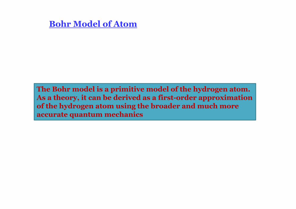
The Bohr model is a primitive model of the hydrogen atom. As a theory, it can be derived as a first-order approximation of the hydrogen atom using the broader and much more accurate quantum mechanics
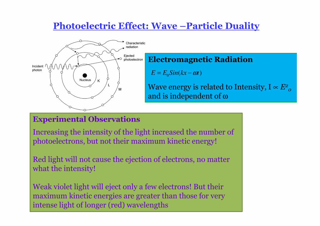
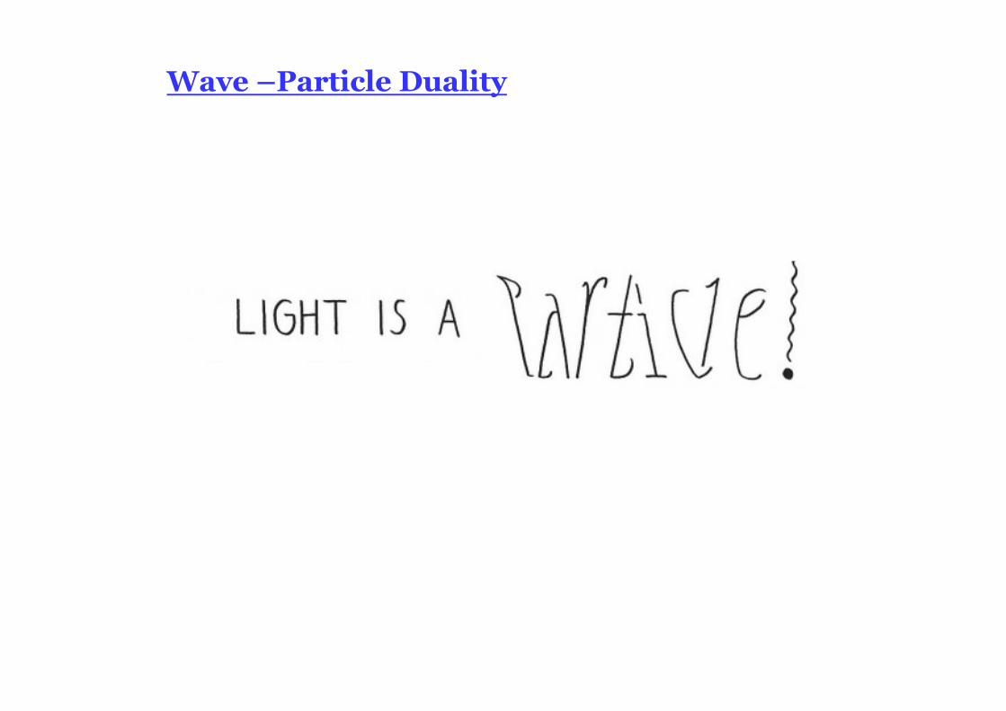
Photoelectric Effect: Wave –Particle Duality
Experimental Observations
Increasing the intensity of the light increased the number of photoelectrons, but not their maximum kinetic energy!
Red light will not cause the ejection of electrons, no matter what the intensity!
Weak violet light will eject only a few electrons! But their maximum kinetic energies are greater than those for very intense light of longer (red) wavelengths
Electromagnetic Radiation
Wave energy is related to Intensity, I ∝ E20and is independent of ω
0 ( )ω= −E E Sin kx t
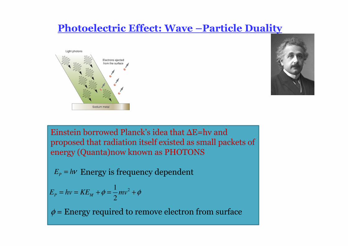
Photoelectric Effect: Wave –Particle Duality
Einstein borrowed Planck’s idea that ∆E=hν and proposed that radiation itself existed as small packets of energy (Quanta)now known as PHOTONS
Energy is frequency dependent
φ = Energy required to remove electron from surface
ν=P
E h
21
2φ φ= = + = +
P ME hv KE mv
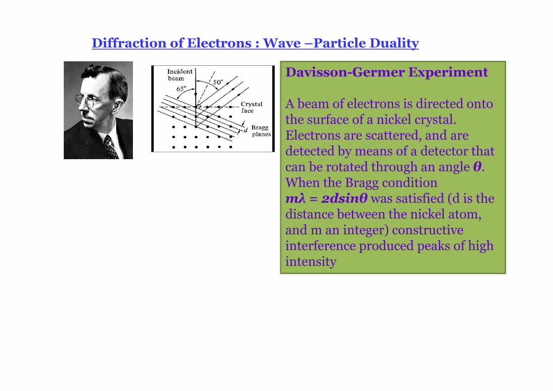
Diffraction of Electrons : Wave –Particle Duality
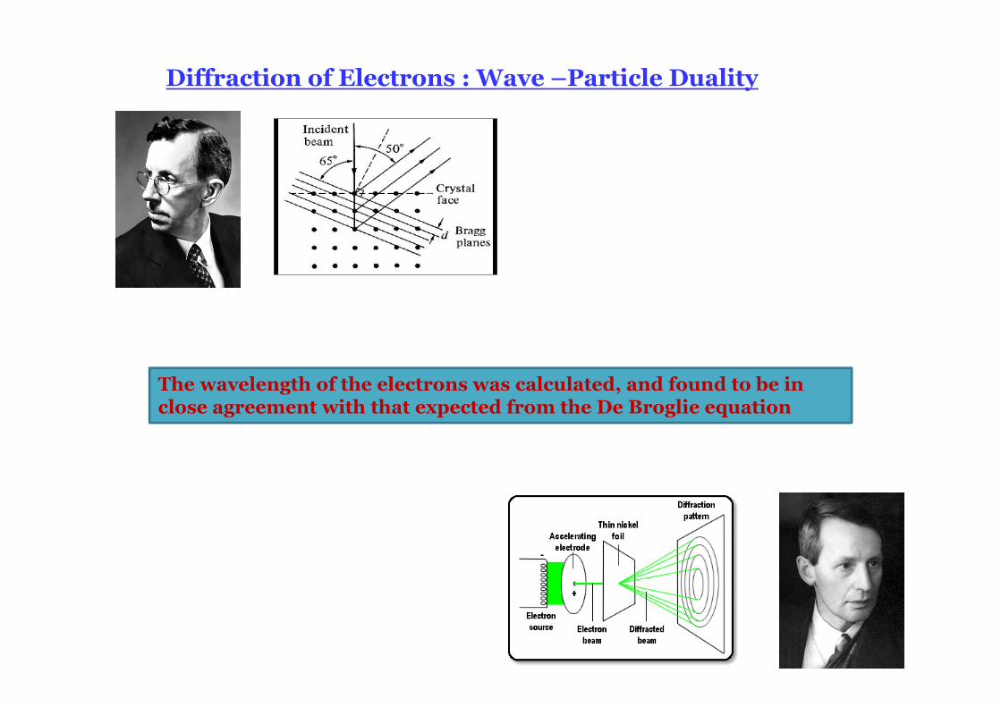
Davisson-Germer Experiment
A beam of electrons is directed onto the surface of a nickel crystal. Electrons are scattered, and are detected by means of a detector that can be rotated through an angle θ. When the Bragg condition mλ = 2dsinθ was satisfied (d is the distance between the nickel atom, and m an integer) constructive interference produced peaks of high intensity
Diffraction of Electrons : Wave –Particle Duality
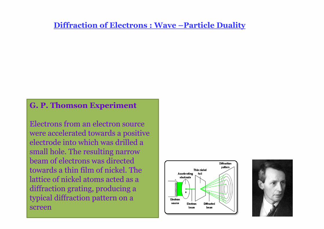
G. P. Thomson Experiment
Electrons from an electron source were accelerated towards a positive electrode into which was drilled a small hole. The resulting narrow beam of electrons was directed towards a thin film of nickel. The lattice of nickel atoms acted as a diffraction grating, producing a typical diffraction pattern on a screen
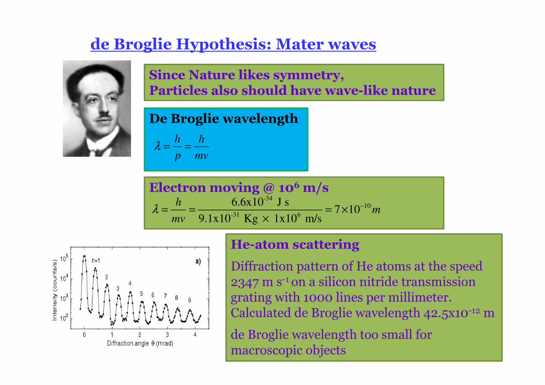
de Broglie Hypothesis: Mater waves
Since Nature likes symmetry, Particles also should have wave-like nature
De Broglie wavelength
λ = =h h
p mv
Electron moving @ 106m/s-34
10
-31 6
6.6x10 J s7 10
9.1x10 Kg 1x10 m/sλ −= = = ×
×
hm
mv
He-atom scattering
Diffraction pattern of He atoms at the speed 2347 m s-1 on a silicon nitride transmission grating with 1000 lines per millimeter. Calculated de Broglie wavelength 42.5x10⁻¹² m
de Broglie wavelength too small for macroscopic objects
Diffraction of Electrons : Wave –Particle Duality
The wavelength of the electrons was calculated, and found to be in close agreement with that expected from the De Broglie equation
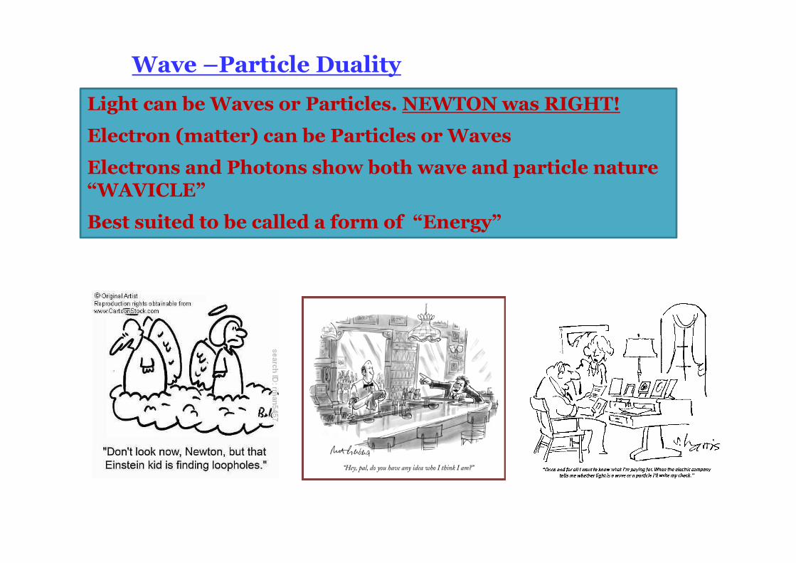
Wave –Particle Duality
Light can be Waves or Particles. NEWTON was RIGHT!
Electron (matter) can be Particles or Waves
Electrons and Photons show both wave and particle nature “WAVICLE”
Best suited to be called a form of “Energy”
Wave –Particle Duality
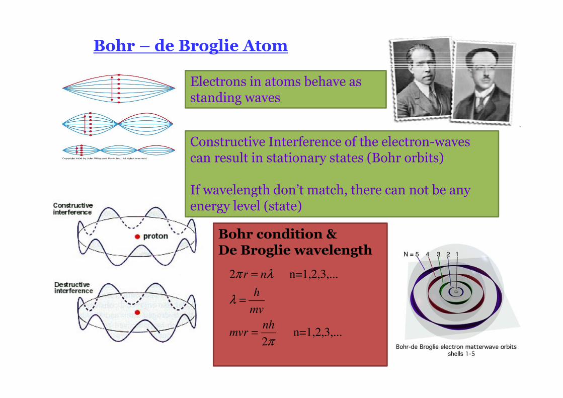
Bohr – de Broglie Atom
Constructive Interference of the electron-waves can result in stationary states (Bohr orbits)
If wavelength don’t match, there can not be any energy level (state)
Bohr condition & De Broglie wavelength
2 n=1,2,3,...
n=1,2,3,...2
π λ
λ
π
=
=
=
r n
h
mv
nhmvr
Electrons in atoms behave as standing waves
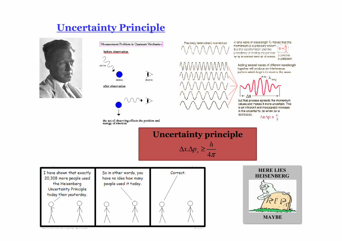
Uncertainty Principle
Uncertainty principle
.4π
∆ ∆ ≥x
hx p
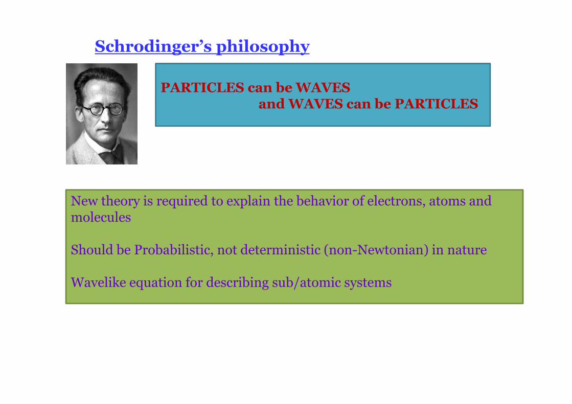
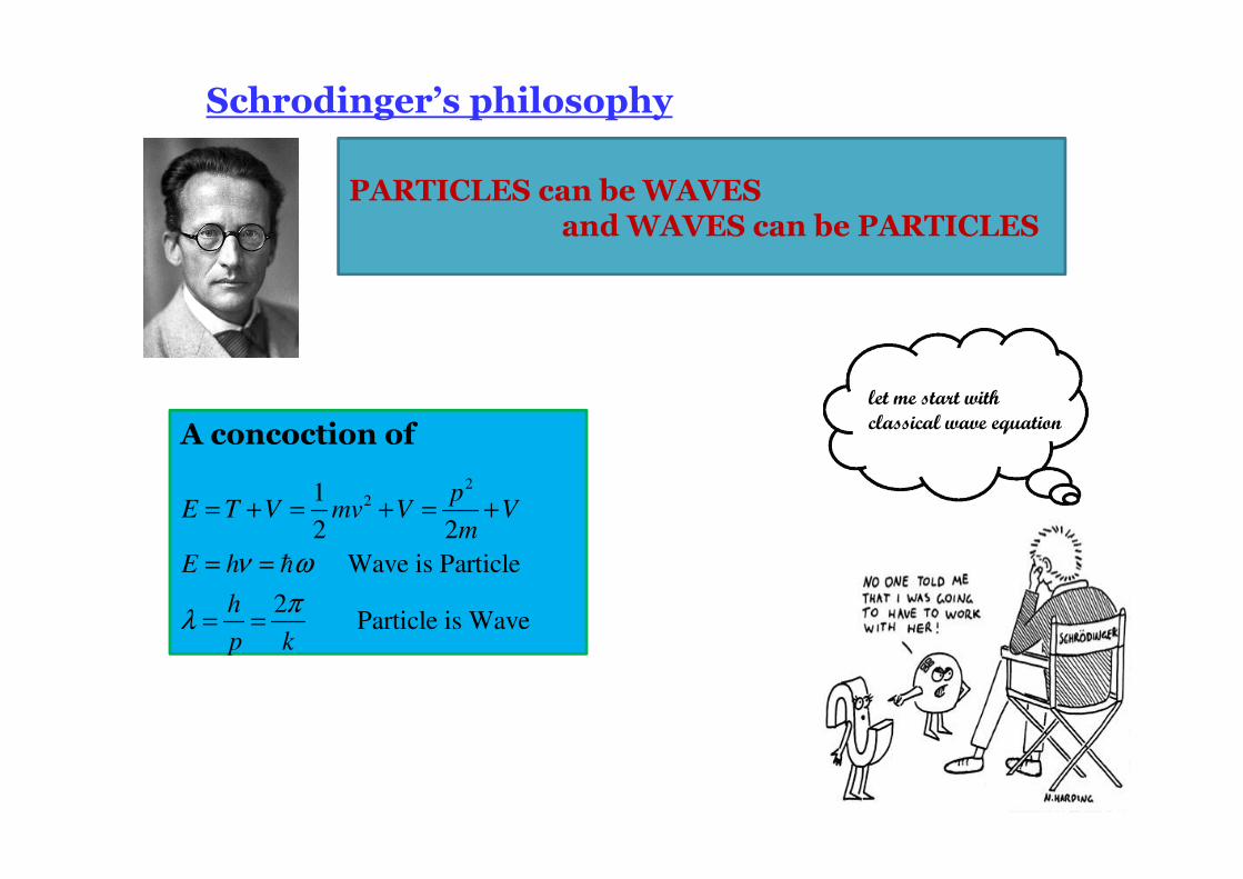
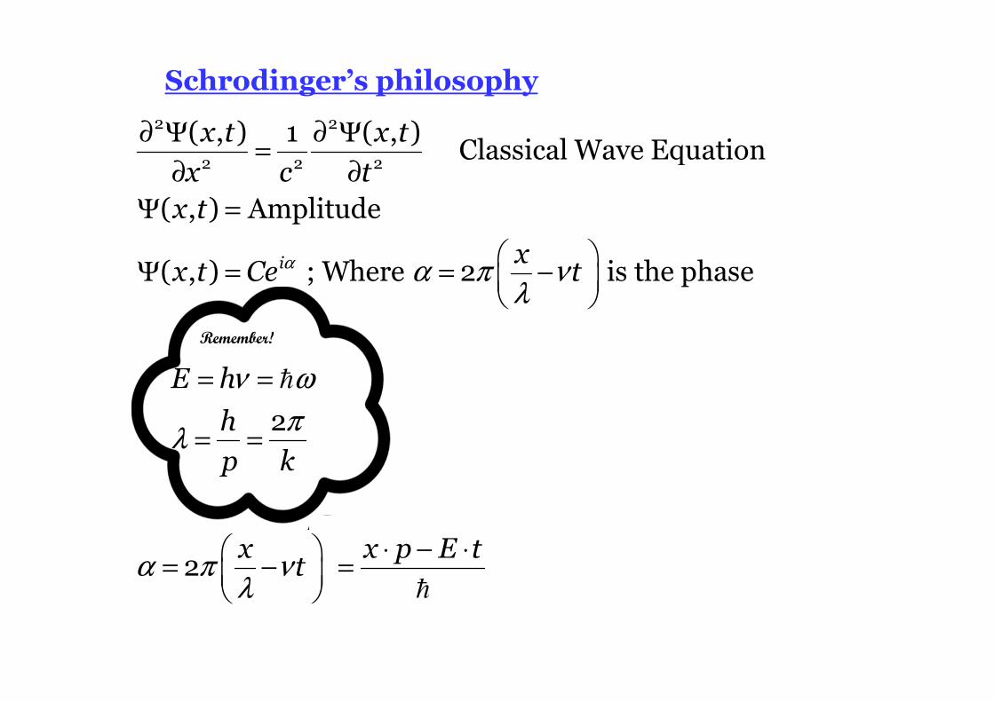
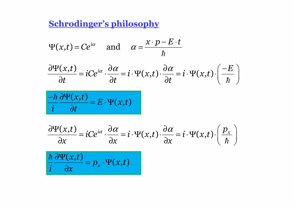
Schrodinger’s philosophy
PARTICLES can be WAVES and WAVES can be PARTICLES
New theory is required to explain the behavior of electrons, atoms and molecules
Should be Probabilistic, not deterministic (non-Newtonian) in nature
Wavelike equation for describing sub/atomic systems
Schrodinger’s philosophy
PARTICLES can be WAVES and WAVES can be PARTICLES
A concoction of
221
2 2
Wave is Particle
2 Particle is Wave
pE T V mv V V
m
E h
h
p k
ν ω
πλ
= + = + = +
= =
= =
�
let me start with classical wave equation
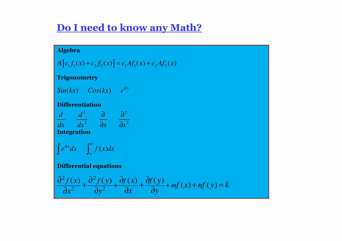
Do I need to know any Math?
Algebra
Trigonometry
Differentiation
Integration
Differential equations
[ ]1 1 2 2 1 1 2 2( ) ( ) ( ) ( )+ = +A c f x c f x c Af x c Af x
( ) ( ) ikx
Sin kx Cos kx e
2 2
2 2
∂ ∂
∂ ∂
d d
dx dx x x
( )∫ ∫b
ikx
ae dx f x dx
2 2
2 2
( ) ( ) ( ) ( )( ) ( )+ +
∂ ∂ ∂ ∂+ + + =
∂ ∂∂ ∂
f f f fm
x y x yf x nf y k
x yx y
Remember!
∂ Ψ ∂ Ψ=
∂ ∂
Ψ =
Ψ = = −
= =
= =
⋅ − ⋅ = − =
�
�
2 2
2 2 2
( , ) 1 ( , ) Classical Wave Equation
( , ) Amplitude
( , ) ; Where 2 is the phase
2
2
i
x t x tx c tx t
xx t Ce t
E h
hp k
x x p E tt
α α π νλ
ν ω
πλ
α π νλ
Schrodinger’s philosophy
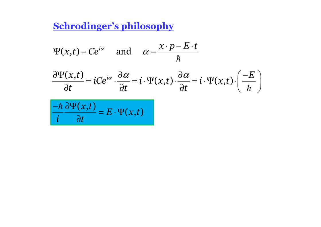
ix t EiCe i x t i x t
t t t
( , )( , ) ( , )α α α∂Ψ ∂ ∂ −
= ⋅ = ⋅Ψ ⋅ = ⋅ Ψ ⋅ ∂ ∂ ∂ �
Schrodinger’s philosophy
x tE x t
i t
( , )( , )
− ∂Ψ= ⋅ Ψ
∂
�
i x p E tx t Ce( , ) and α α
⋅ − ⋅Ψ = =
�
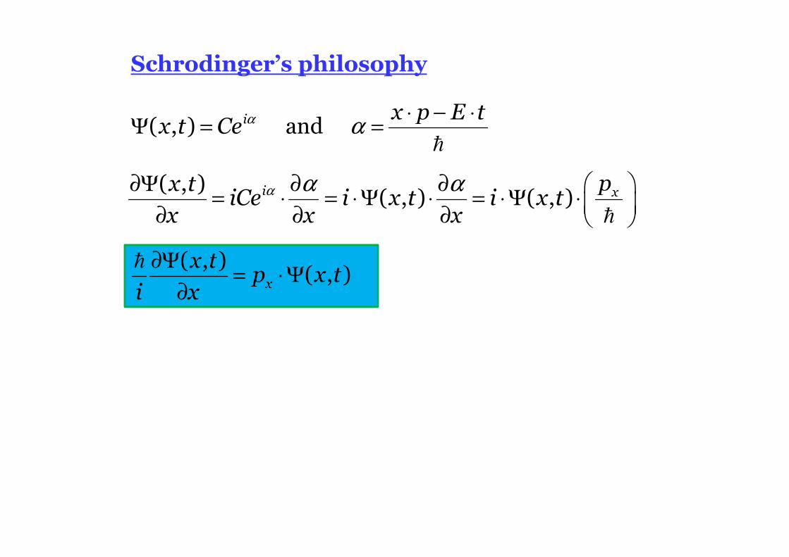
Schrodinger’s philosophy
∂Ψ= ⋅ Ψ
∂
� ( , )( , ) x
x tp x t
i x
i x p E tx t Ce( , ) and α α
⋅ − ⋅Ψ = =
�
α α α∂Ψ ∂ ∂ = ⋅ = ⋅Ψ ⋅ = ⋅Ψ ⋅ ∂ ∂ ∂ �
( , )( , ) ( , )i xpx t
iCe i x t i x tx x x
ix t EiCe i x t i x t
t t t
( , )( , ) ( , )α α α∂Ψ ∂ ∂ −
= ⋅ = ⋅Ψ ⋅ = ⋅ Ψ ⋅ ∂ ∂ ∂ �
Schrodinger’s philosophy
x tE x t
i t
( , )( , )
− ∂Ψ= ⋅ Ψ
∂
�
i xpx tiCe i x t i x t
x x x( , )
( , ) ( , )α α α∂Ψ ∂ ∂ = ⋅ = ⋅Ψ ⋅ = ⋅Ψ ⋅ ∂ ∂ ∂ �
x
x tp x t
i x( , )
( , )∂Ψ
= ⋅Ψ∂
�
i x p E tx t Ce( , ) and α α
⋅ − ⋅Ψ = =
�
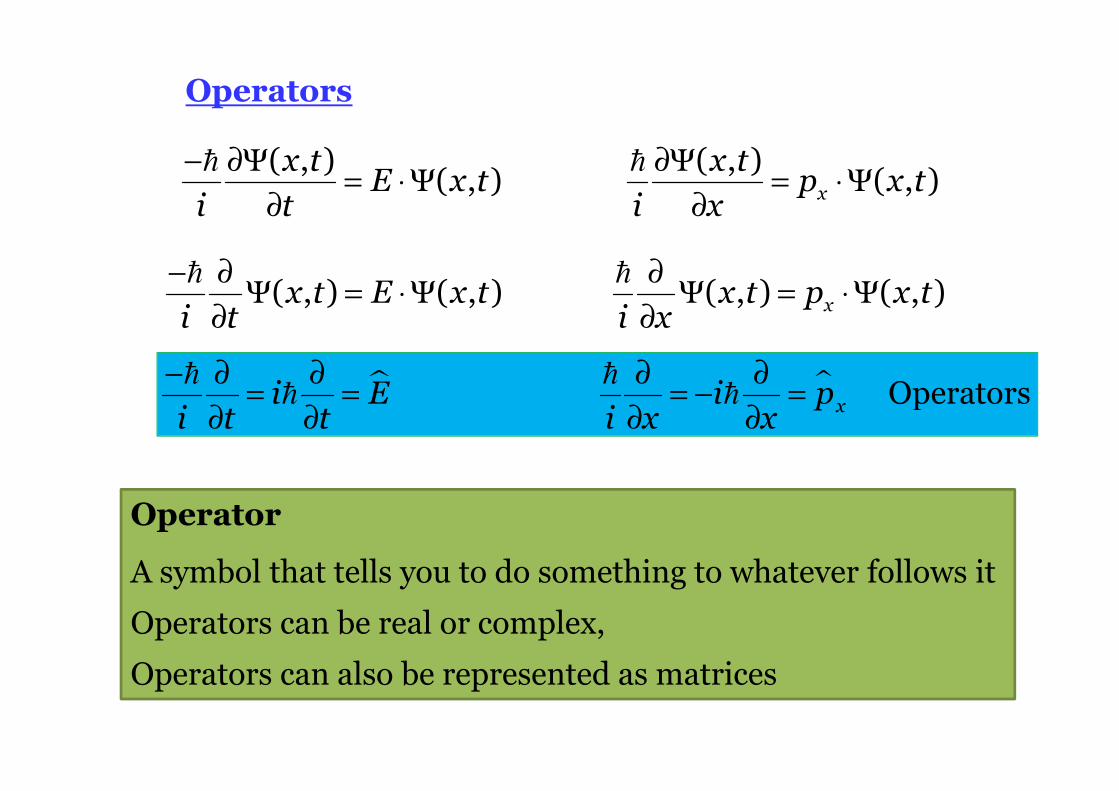
� �− ∂ ∂ ∂ ∂= = = − =
∂ ∂ ∂ ∂
� �� � Operatorsxi E i p
i t t i x x
Operators
x
x t x tE x t p x t
i t i x
( , ) ( , )( , ) ( , )
− ∂Ψ ∂Ψ= ⋅ Ψ = ⋅Ψ
∂ ∂
� �
Operator
A symbol that tells you to do something to whatever follows it
Operators can be real or complex,
Operators can also be represented as matrices
xx t E x t x t p x ti t i x
( , ) ( , ) ( , ) ( , )− ∂ ∂
Ψ = ⋅Ψ Ψ = ⋅Ψ∂ ∂
� �
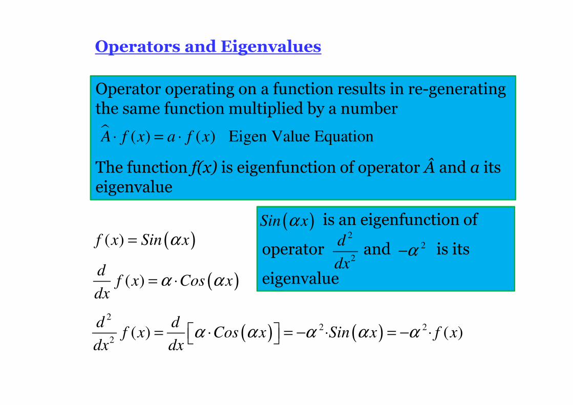
Operators and Eigenvalues
Operator operating on a function results in re-generating the same function multiplied by a number
The function f(x) is eigenfunction of operator  and a its eigenvalue
( )( ) α=f x Sin x
( )( ) α α= ⋅d
f x Cos xdx
( ) ( )2
2 2
2( ) ( )α α α α α= ⋅ = − ⋅ = − ⋅
d df x Cos x Sin x f x
dx dx
is an eigenfunction of
operator and is its
eigenvalue
( )αSin x2
2
d
dx
2α−
� ( ) ( ) Eigen Value EquationA f x a f x⋅ = ⋅
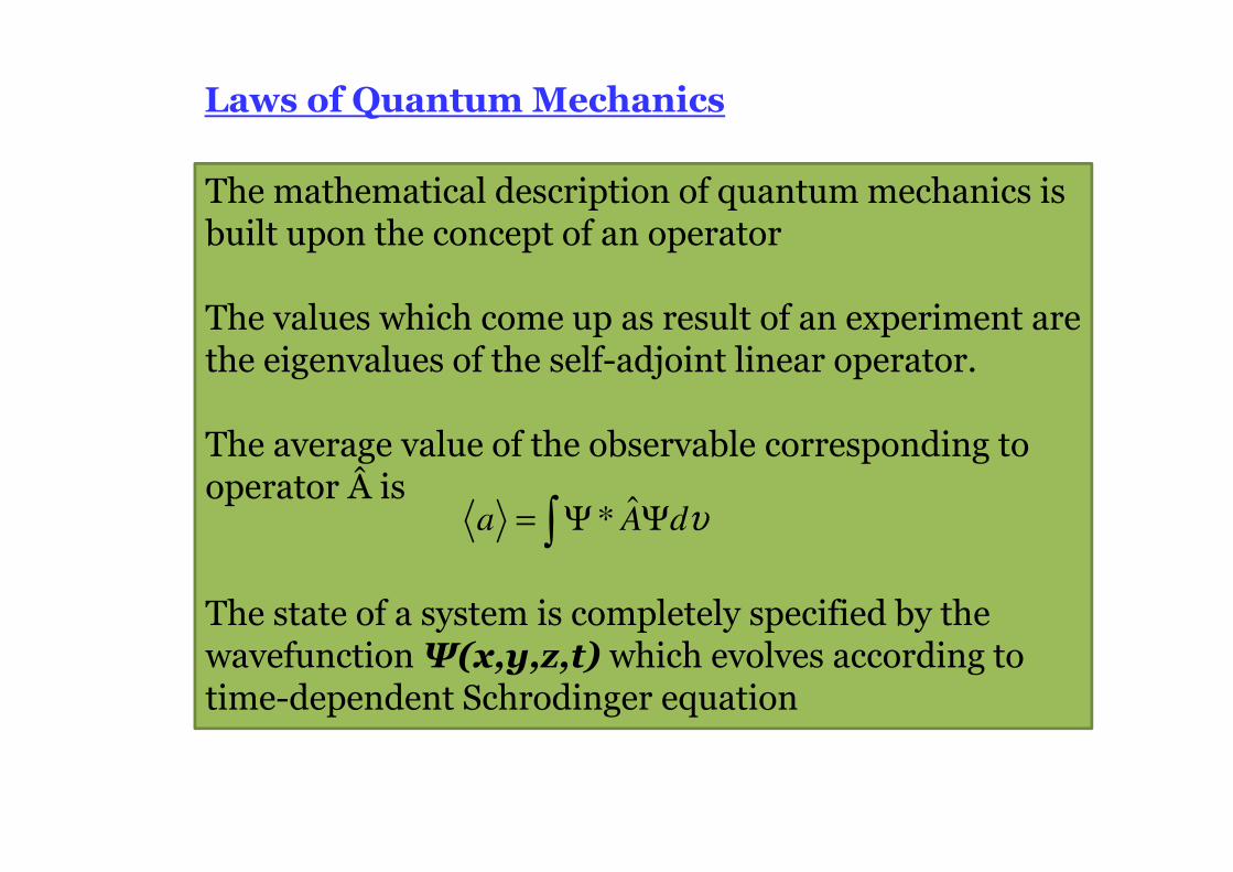
The mathematical description of quantum mechanics is built upon the concept of an operator
The values which come up as result of an experiment are the eigenvalues of the self-adjoint linear operator.
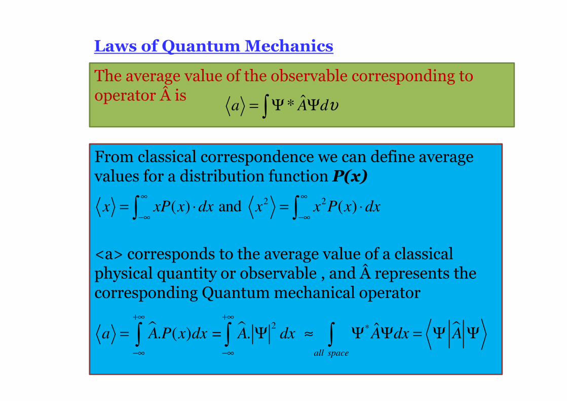
The average value of the observable corresponding to operator  is
The state of a system is completely specified by the wavefunction Ψ(x,y,z,t) which evolves according to time-dependent Schrodinger equation
Laws of Quantum Mechanics
ˆ* υ= Ψ Ψ∫a A d
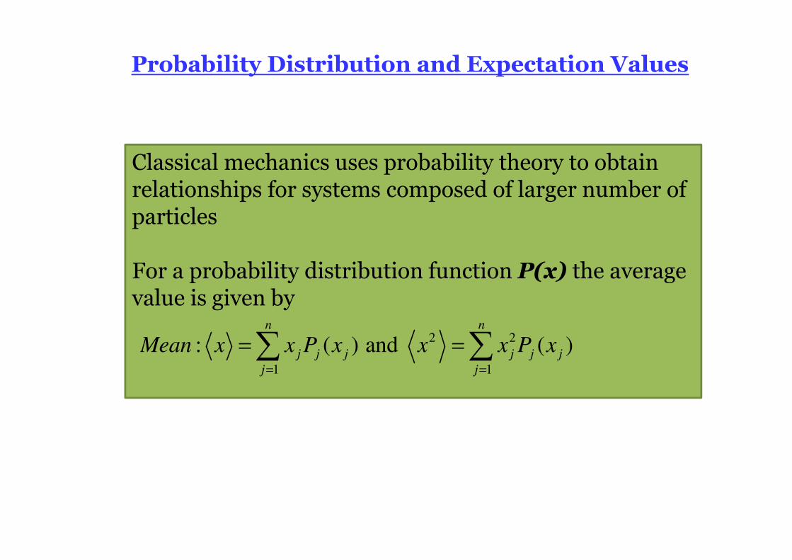
Probability Distribution and Expectation Values
Classical mechanics uses probability theory to obtain relationships for systems composed of larger number of particles
For a probability distribution function P(x) the average value is given by
2 2
1 1
: ( ) and ( )= =
= =∑ ∑n n
j j j j j j
j j
Mean x x P x x x P x
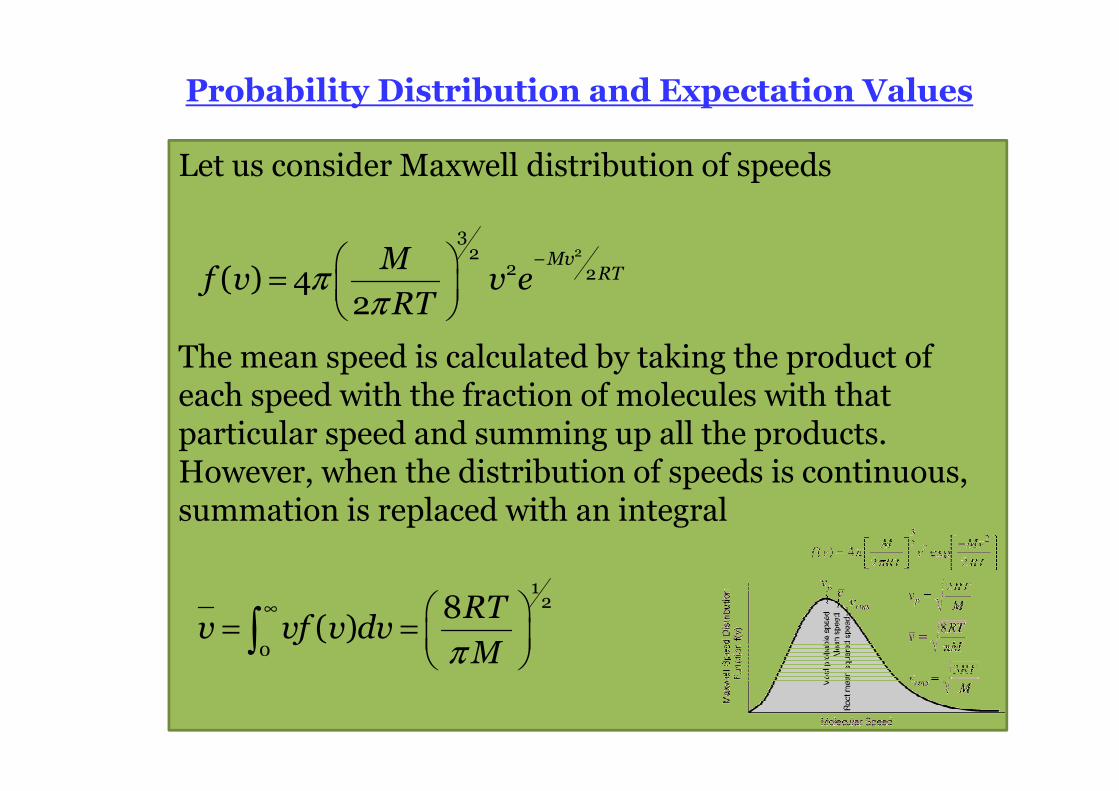
Let us consider Maxwell distribution of speeds
The mean speed is calculated by taking the product of each speed with the fraction of molecules with that particular speed and summing up all the products. However, when the distribution of speeds is continuous, summation is replaced with an integral
RTv vf v dv
M
12
0
8( )
π
∞ = =
∫
MvRT
Mf v v e
RT
232
2 2( ) 42
ππ
− =
Probability Distribution and Expectation Values
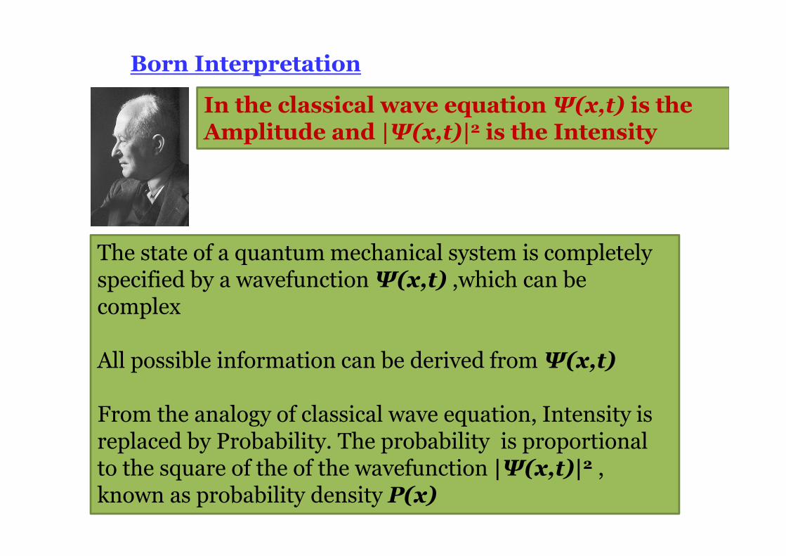
Born Interpretation
In the classical wave equation Ψ(x,t) is the Amplitude and |Ψ(x,t)|2 is the Intensity
The state of a quantum mechanical system is completely specified by a wavefunction Ψ(x,t) ,which can be complex
All possible information can be derived from Ψ(x,t)
From the analogy of classical wave equation, Intensity is replaced by Probability. The probability is proportional to the square of the of the wavefunction |Ψ(x,t)|2 , known as probability density P(x)
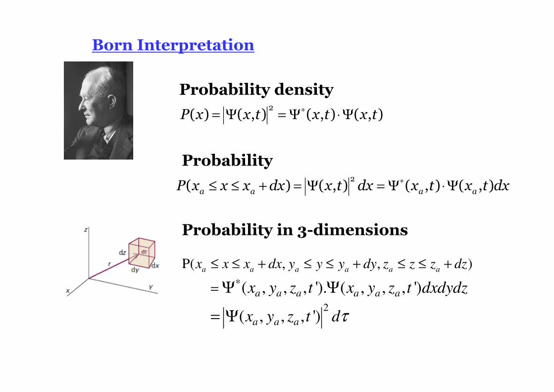
Born Interpretation
P x x t x t x t2
( ) ( , ) ( , ) ( , )∗= Ψ = Ψ ⋅Ψ
Probability density
Probability
a a a aP x x x dx x t dx x t x t dx2
( ) ( , ) ( , ) ( , )∗≤ ≤ + = Ψ = Ψ ⋅Ψ
Probability in 3-dimensions
*
2
P( , , )
( , , , '). ( , , , ')
( , , , ') τ
≤ ≤ + ≤ ≤ + ≤ ≤ +
= Ψ Ψ
= Ψ
a a a a a a
a a a a a a
a a a
x x x dx y y y dy z z z dz
x y z t x y z t dxdydz
x y z t d
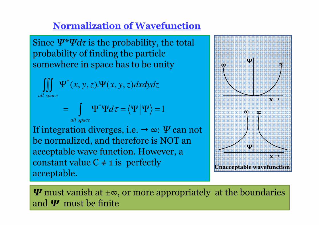
Normalization of Wavefunction
∞∞
x�
Ψ
∞∞
x�
Ψ
Unacceptable wavefunction
Since Ψ*Ψdτ is the probability, the total probability of finding the particle somewhere in space has to be unity
If integration diverges, i.e. � ∞: Ψ can not be normalized, and therefore is NOT an acceptable wave function. However, a constant value C ≠ 1 is perfectly acceptable.
*
*
( , , ). ( , , )
1τ
Ψ Ψ
= Ψ Ψ = Ψ Ψ =
∫∫∫
∫
all space
all space
x y z x y z dxdydz
d
Ψ must vanish at ±∞, or more appropriately at the boundaries and Ψ must be finite
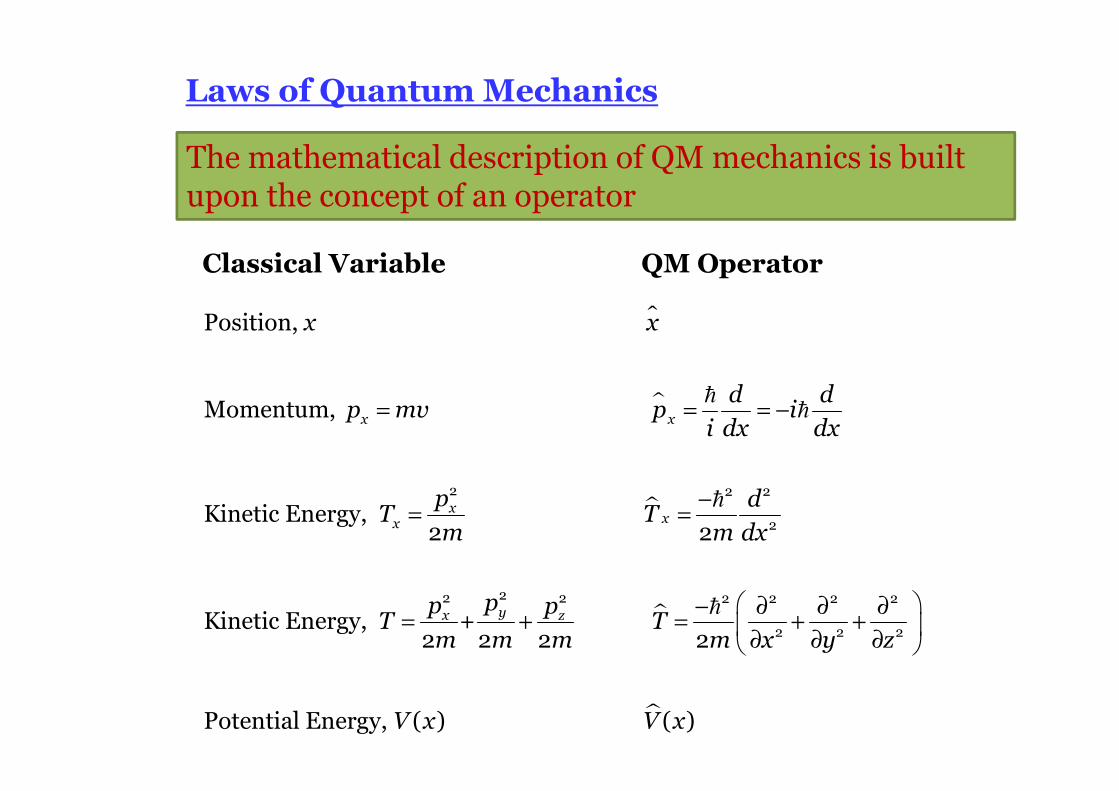
Laws of Quantum Mechanics
�
�xx
xx
x x
d dp mv p i
i dx dx
pT
m
2
Position,
Momentum,
Kinetic Energy, 2
= = = −
=
��
�
�
�
x
yx z
dT
m dx
pp pT T
m m m m x y z
V x V x
2 2
2
22 2 2 2 2 2
2 2 2
2
Kinetic Energy, + 2 2 2 2
Potential Energy, ( ) ( )
−=
− ∂ ∂ ∂= + = + +
∂ ∂ ∂
�
�
Classical Variable QM Operator
The mathematical description of QM mechanics is built upon the concept of an operator
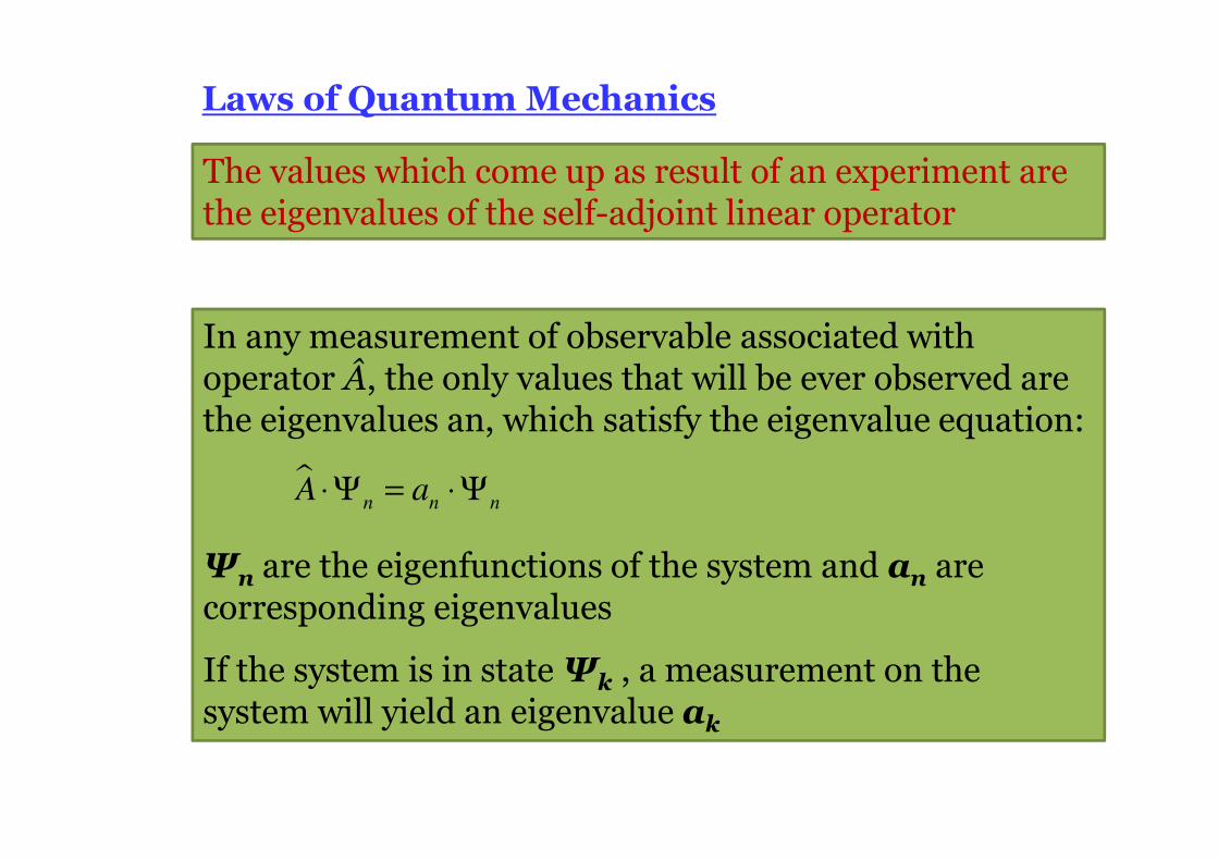
Laws of Quantum Mechanics
The values which come up as result of an experiment are the eigenvalues of the self-adjoint linear operator
In any measurement of observable associated with operator Â, the only values that will be ever observed are the eigenvalues an, which satisfy the eigenvalue equation:
Ψn are the eigenfunctions of the system and an are corresponding eigenvalues
If the system is in state Ψk , a measurement on the system will yield an eigenvalue ak
� ⋅Ψ = ⋅ Ψn n nA a
Laws of Quantum Mechanics
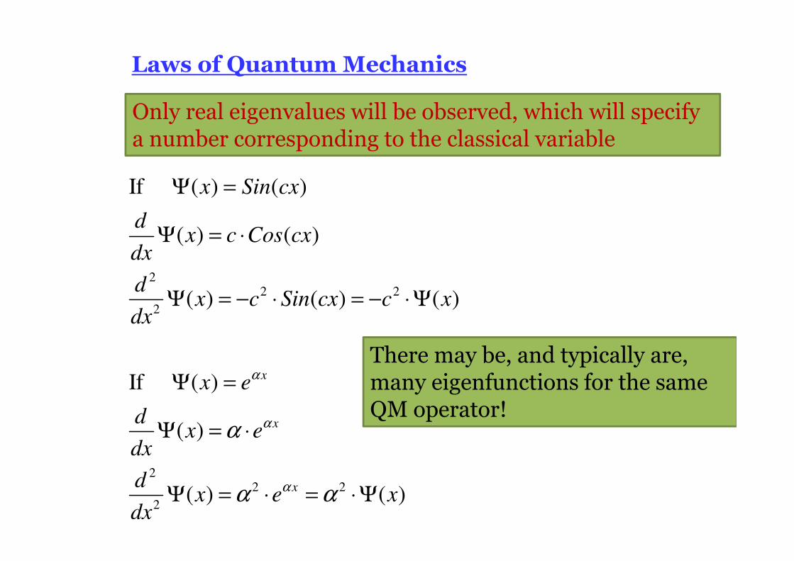
22 2
2
22 2
2
If ( ) ( )
( ) ( )
( ) ( ) ( )
If ( )
( )
( ) ( )
x
x
x
x Sin cx
dx c Cos cx
dx
dx c Sin cx c x
dx
x e
dx e
dx
dx e x
dx
α
α
α
α
α α
Ψ =
Ψ = ⋅
Ψ = − ⋅ = − ⋅Ψ
Ψ =
Ψ = ⋅
Ψ = ⋅ = ⋅Ψ
Only real eigenvalues will be observed, which will specify a number corresponding to the classical variable
There may be, and typically are, many eigenfunctions for the same QM operator!
Laws of Quantum Mechanics
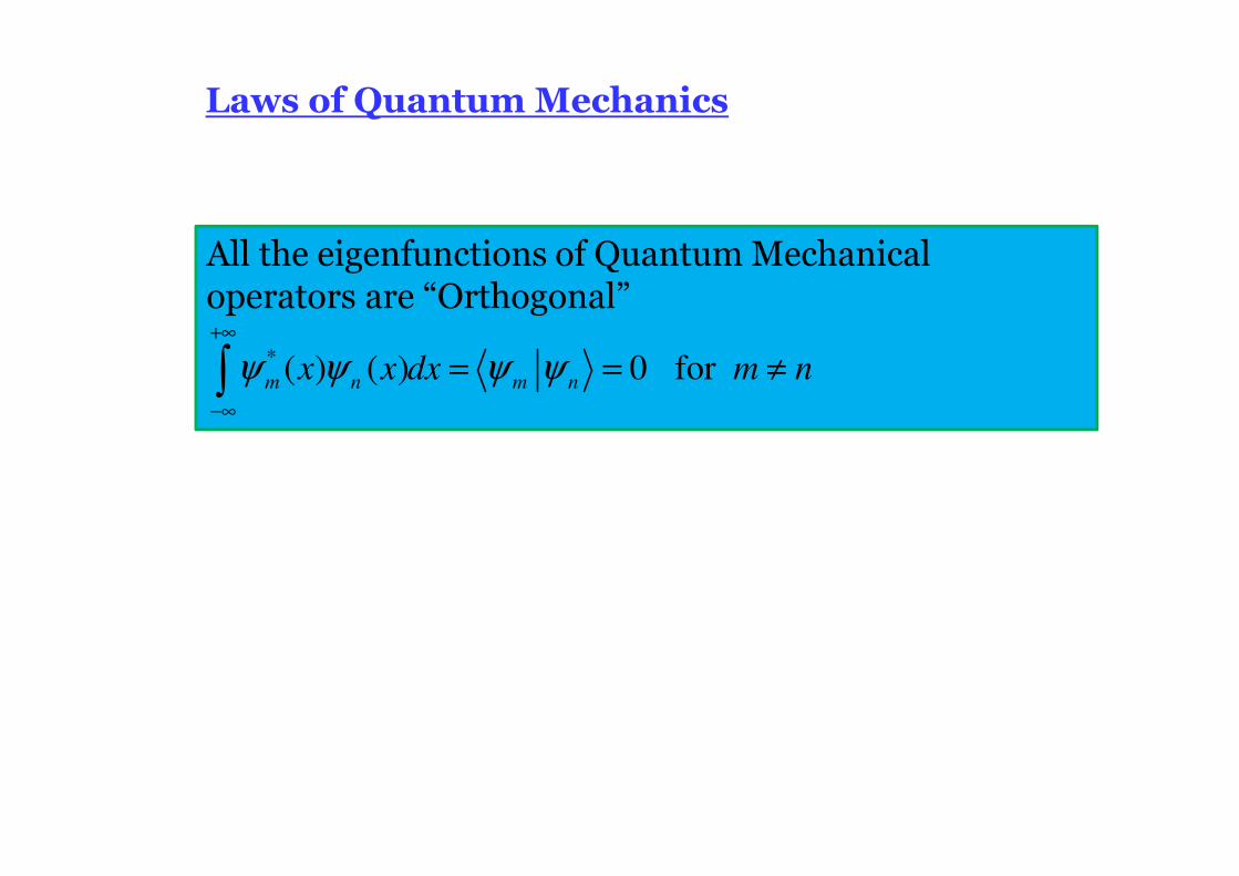
All the eigenfunctions of Quantum Mechanical operators are “Orthogonal”
* ( ) ( ) 0 for ψ ψ ψ ψ+∞
−∞
= = ≠∫ m n m nx x dx m n
Laws of Quantum Mechanics
The average value of the observable corresponding to operator  is ˆ* υ= Ψ Ψ∫a A d
From classical correspondence we can define average values for a distribution function P(x)
<a> corresponds to the average value of a classical physical quantity or observable , and  represents the corresponding Quantum mechanical operator
2 2( ) and ( ) ∞ ∞
−∞ −∞= ⋅ = ⋅∫ ∫x xP x dx x x P x dx
� � �2 *
ˆ. ( ) = .
+∞ +∞
−∞ −∞
= Ψ ≈ Ψ Ψ = Ψ Ψ∫ ∫ ∫all space
a A P x dx A dx A dx A
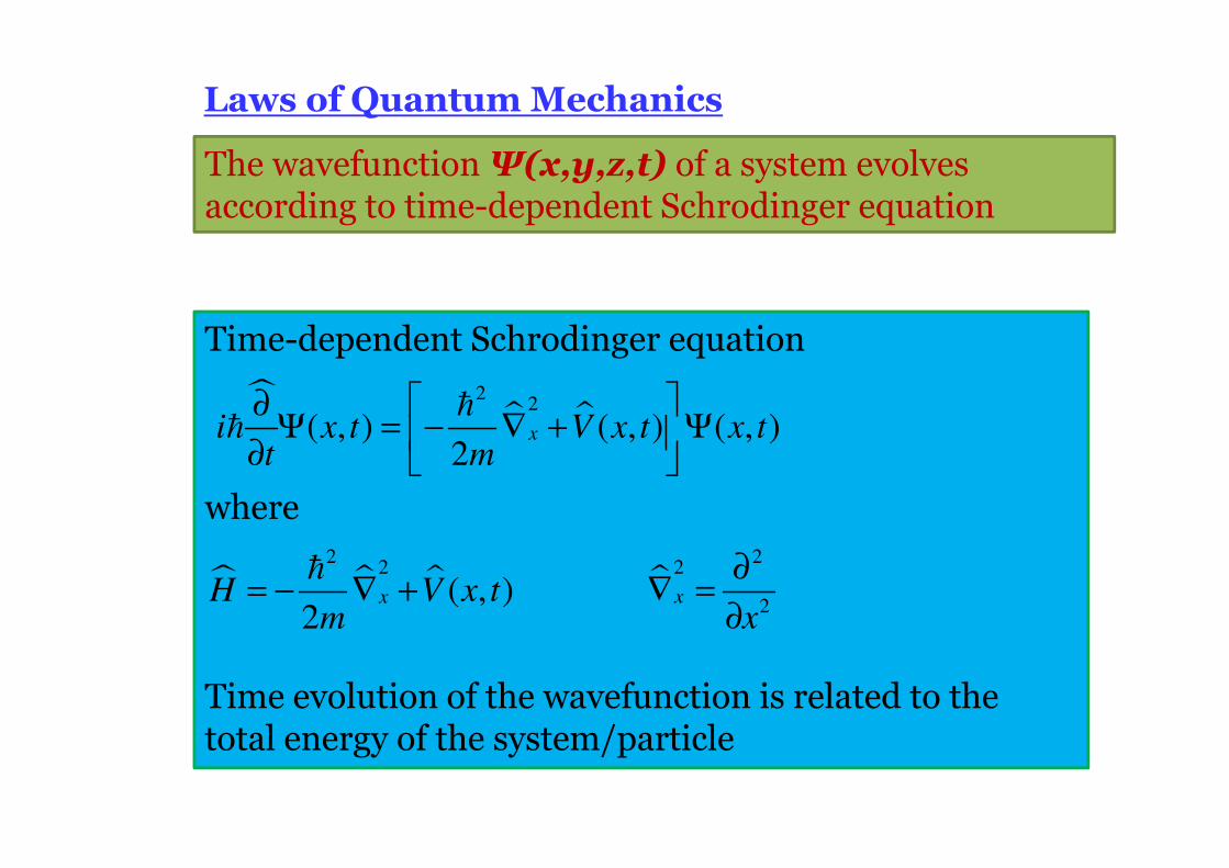
Time-dependent Schrodinger equation
where
Time evolution of the wavefunction is related to the total energy of the system/particle
Laws of Quantum Mechanics
�� �
22
( , ) ( , ) ( , )2
∂Ψ = − ∇ + Ψ
∂
�� xi x t V x t x t
t m
� � �2
2
( , )2
= − ∇ +�
xH V x tm
�2
2
2
∂∇ =
∂x
x
The wavefunction Ψ(x,y,z,t) of a system evolves according to time-dependent Schrodinger equation
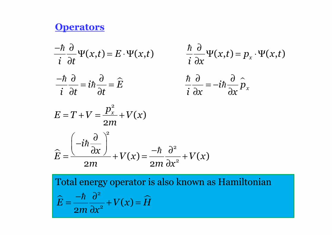
Operators
� �xi E i p
i t t i x x
− ∂ ∂ ∂ ∂= = = −
∂ ∂ ∂ ∂
� �� �
xx t E x t x t p x ti t i x
( , ) ( , ) ( , ) ( , )− ∂ ∂
Ψ = ⋅Ψ Ψ = ⋅Ψ∂ ∂
� �
Total energy operator is also known as Hamiltonian
� �E V x Hm x
2
2( )
2
− ∂= + =
∂
�
�
xpE T V V xm
ix
E V x V xm m x
2
2
2
2
( )2
( ) ( )2 2
= + = +
∂ − − ∂∂ = + = +
∂
��
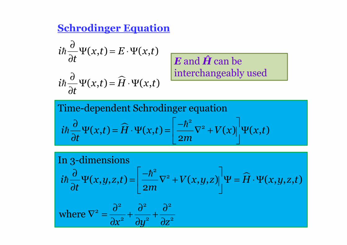
Schrodinger Equation
Time-dependent Schrodinger equation
�i x t H x t V x x tt m
22( , ) ( , ) ( ) ( , )
2
∂ −Ψ = ⋅Ψ = ∇ + Ψ
∂
��
In 3-dimensions
�i x y z t V x y z H x y z tt m
22( , , , ) ( , , ) ( , , , )
2
∂ −Ψ = ∇ + Ψ = ⋅Ψ
∂
��
x y z
2 2 22
2 2 2where
∂ ∂ ∂∇ = + +
∂ ∂ ∂
�i x t H x tt
( , ) ( , )∂
Ψ = ⋅ Ψ∂�
E and Ĥ can be interchangeably used
i x t E x tt
( , ) ( , )∂
Ψ = ⋅Ψ∂�
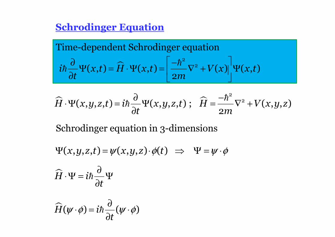
Schrodinger Equation
Time-dependent Schrodinger equation
�i x t H x t V x x tt m
22( , ) ( , ) ( ) ( , )
2
∂ −Ψ = ⋅Ψ = ∇ + Ψ
∂
��
� �H x y z t i x y z t H V x y zt m
22( , , , ) ( , , , ) ; ( , , )
2∂ −
⋅ Ψ = Ψ = ∇ +∂
��
x y z t x y z t( , , , ) ( , , ) ( ) ψ φ ψ φΨ = ⋅ ⇒ Ψ = ⋅
Schrodinger equation in 3-dimensions
�H it
∂⋅ Ψ = Ψ
∂�
�H it
( ) ( )ψ φ ψ φ∂
⋅ = ⋅∂�
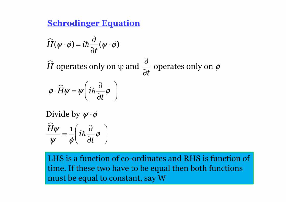
Schrodinger Equation
�
�
H it
Ht
( ) ( )
operates only on ψ and operates only on
ψ φ ψ φ
φ
∂⋅ = ⋅
∂
∂
∂
�
�H it
φ ψ ψ φ∂
⋅ = ∂ �
�Hit
Divide by
1
ψ φ
ψφ
ψ φ
⋅
∂ =
∂ �
LHS is a function of co-ordinates and RHS is function of time. If these two have to be equal then both functions must be equal to constant, say W
Schrodinger Equation
�Hi Wt
1ψφ
ψ φ
∂ = =
∂ �
��H
W H W
i W i Wt t
1
ψψ ψ
ψ
φ φ φφ
⋅= =
∂ ∂ = =
∂ ∂ � �
The solution of the differential equationiWt
i W t et
is ( )φ φ φ−∂
= =∂
��
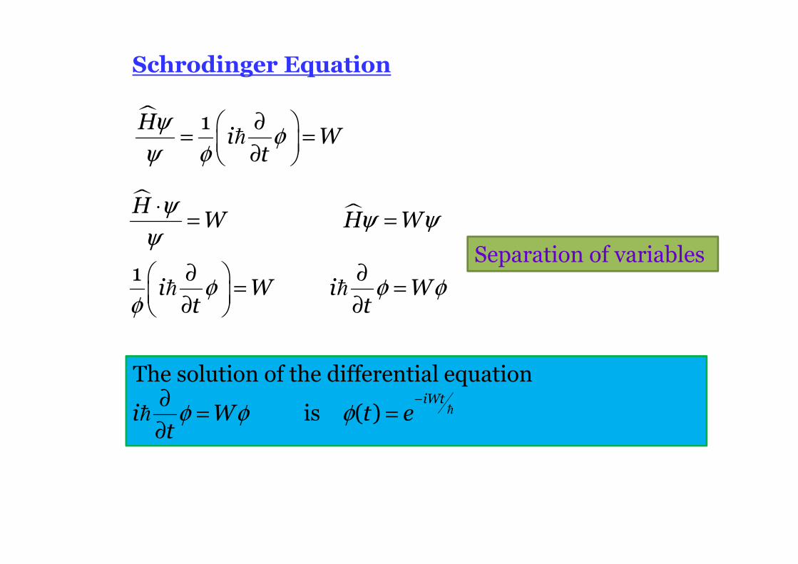
Separation of variables
Schrodinger Equation
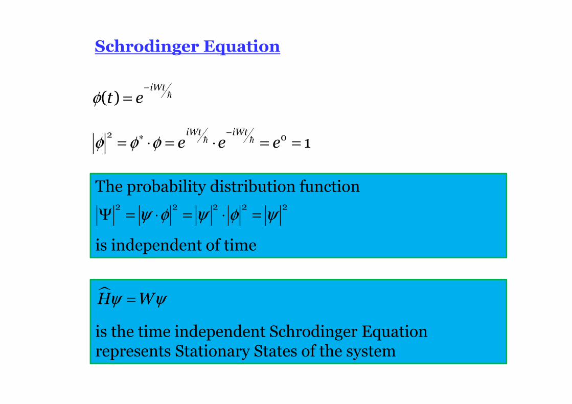
iWtt e( )φ
−
= �
iWt iWte e e
2 0 1φ φ φ−
∗= ⋅ = ⋅ = =� �
The probability distribution function
is independent of time
2 2 2 2 2ψ φ ψ φ ψΨ = ⋅ = ⋅ =
is the time independent Schrodinger Equation represents Stationary States of the system
�H Wψ ψ=
Schrodinger Equation
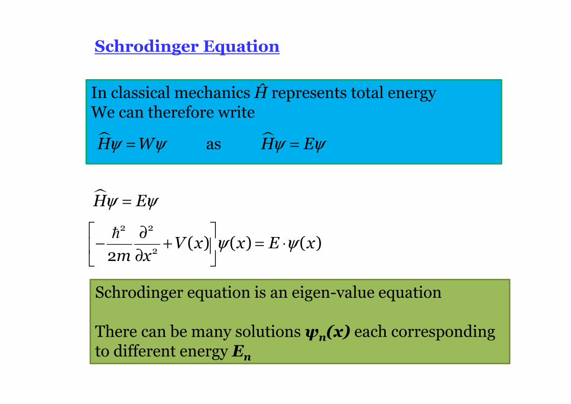
In classical mechanics Ĥ represents total energyWe can therefore write
� �H W H E as ψ ψ ψ ψ= =
�H Eψ ψ=
V x x E xm x
2 2
2( ) ( ) ( )
2ψ ψ
∂− + = ⋅
∂
�
Schrodinger equation is an eigen-value equation
There can be many solutions ψn(x) each corresponding to different energy En
Schrodinger Equation
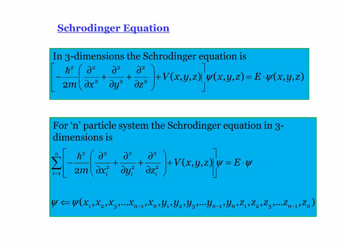
In 3-dimensions the Schrodinger equation is
V x y z x y z E x y zm x y z
2 2 2 2
2 2 2( , , ) ( , , ) ( , , )
2ψ ψ
∂ ∂ ∂− + + + = ⋅
∂ ∂ ∂
�
For ‘n’ particle system the Schrodinger equation in 3-dimensions is
ψ ψ
ψ ψ
=
− − −
∂ ∂ ∂− + + + = ⋅
∂ ∂ ∂
⇐
∑�2 2 2 2
2 2 21
1 2 3 1 1 2 3 1 1 2 3 1
( , , )2
( , , ,... , , , , ,... , , , , ,... , )
n
i i i i
n n n n n n
V x y z Em x y z
x x x x x y y y y y z z z z z
Schrodinger Equation
�
ψ ψ
∂ ∂ ∂= − + +
∂ ∂ ∂
∂ ∂ ∂− + +
∂ ∂ ∂
∂ ∂ ∂− + + ∂ ∂ ∂
∂ ∂ ∂− + + ∂ ∂ ∂
+ + + + + +
⇐
�
�
�
�
2 2 2 2
2 2 21 1 1 1
2 2 2 2
2 2 22 2 2 2
2 2 2 2
2 2 23 3 3 3
2 2 2 2
2 2 24 4 4 4
12 13 14 23 24 34
1 2 3
2
2
2
2
( , , ,
Hm x y z
m x y z
m x y z
m x y z
V V V V V V
x x x x4 1 2 3 4 1 2 3 4, , , , , , , , )y y y y z z z z
( )1 1 1 1, ,m x y z
( )3 3 3 3, ,m x y z( )2 2 2 2, ,m x y z
( )4 4 4 4, ,m x y z
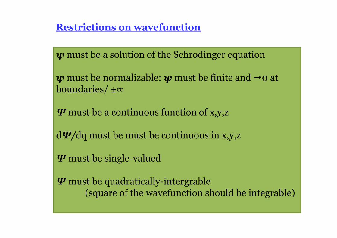
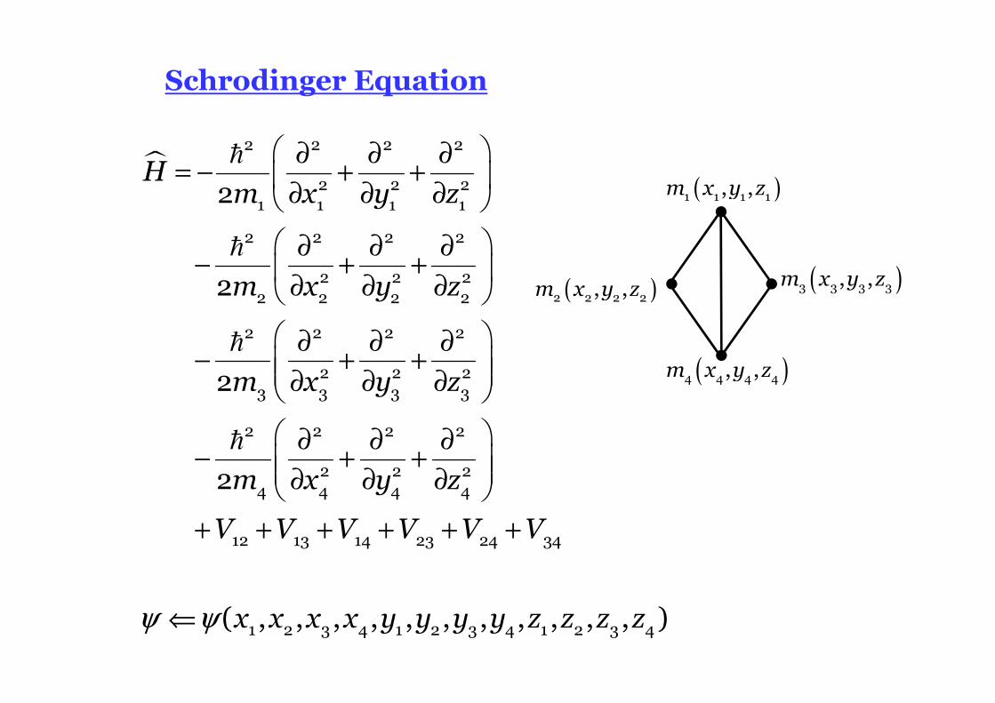
Restrictions on wavefunction
ψ must be a solution of the Schrodinger equation
ψ must be normalizable: ψ must be finite and �0 at boundaries/ ±∞
Ψ must be a continuous function of x,y,z
dΨ/dq must be must be continuous in x,y,z
Ψ must be single-valued
Ψ must be quadratically-intergrable(square of the wavefunction should be integrable)
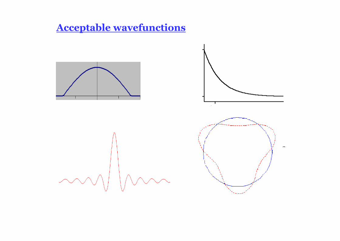
Acceptable wavefunctions
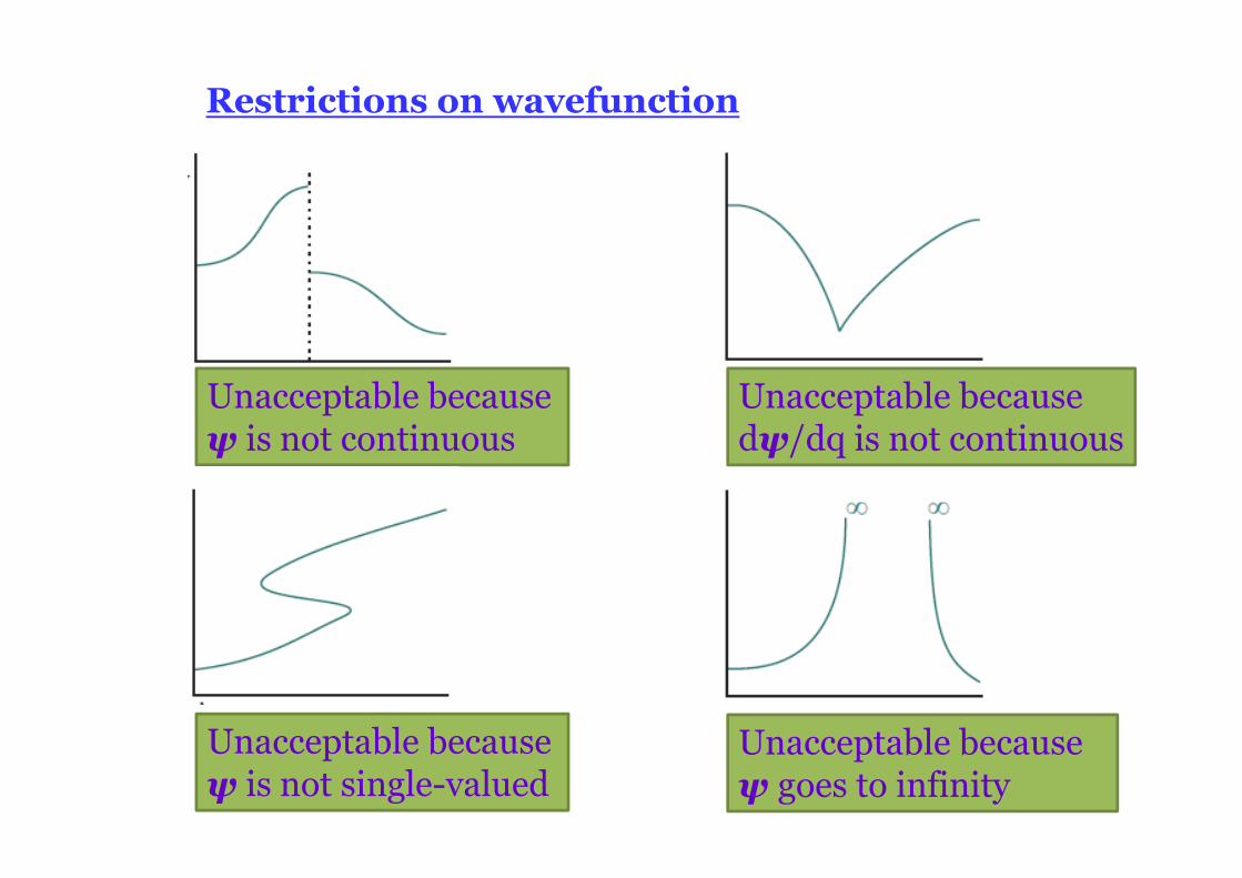
Restrictions on wavefunction
Unacceptable because ψ is not continuous
Unacceptable because ψ is not single-valued
Unacceptable because dψ/dq is not continuous
Unacceptable because ψ goes to infinity
Restrictions on wavefunction
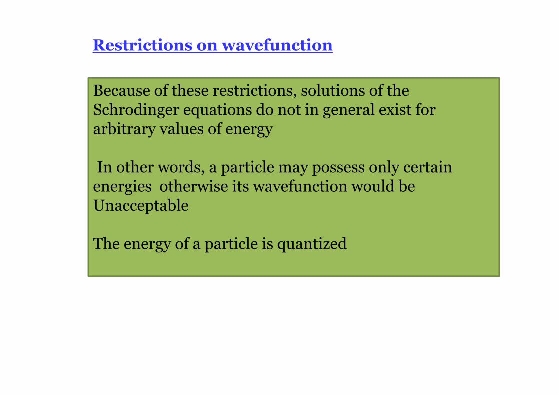
Because of these restrictions, solutions of the Schrodinger equations do not in general exist for arbitrary values of energy
In other words, a particle may possess only certain energies otherwise its wavefunction would be Unacceptable
The energy of a particle is quantized
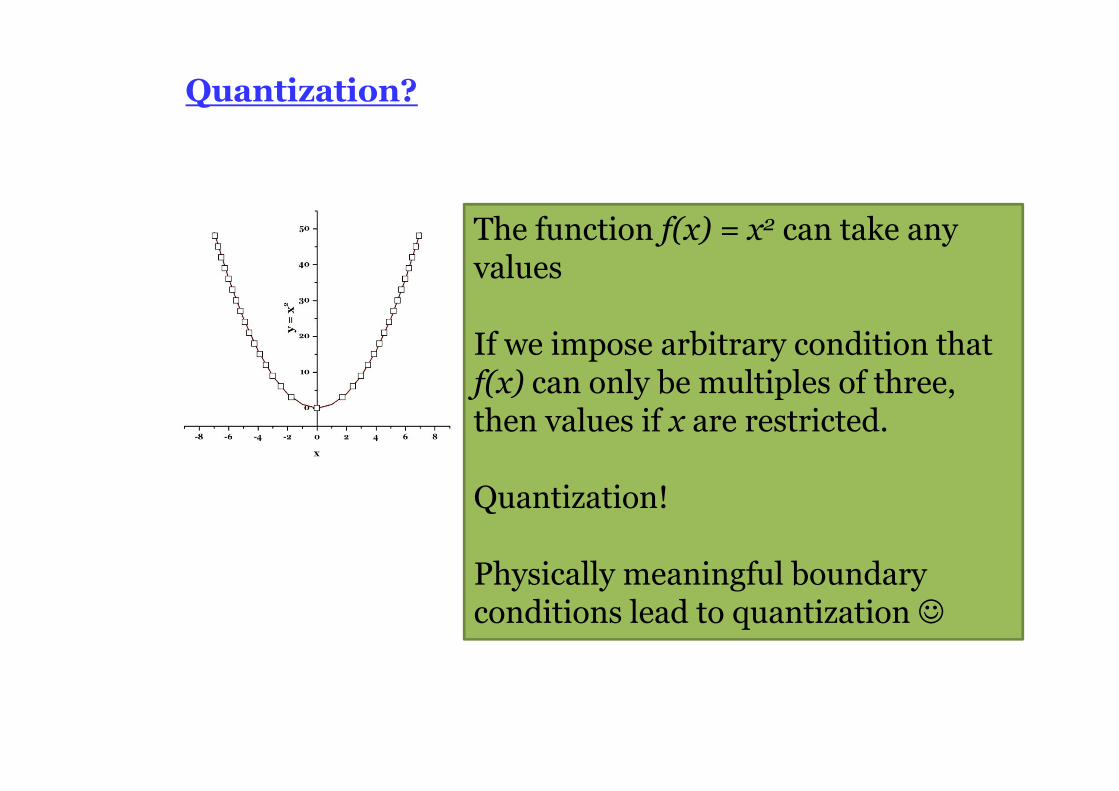
Quantization?
The function f(x) = x2 can take any values
If we impose arbitrary condition that f(x) can only be multiples of three, then values if x are restricted.
Quantization!
Physically meaningful boundary conditions lead to quantization ☺
Not deterministic: Can not precisely determine many parameters in the system, but Ψ can provide all the information (spatio-temporal) of a system.
Only average values and probabilities can be obtained for classical variables, now in new form of “operators”.
Total energy is conserved, but quantization of energy levels come spontaneously from restriction on wave function or boundary condition
Final outputs tally very well with experimental results, and does not violate Classical mechanics for large value of mass.
Essence of Quantum Mechanics
Quantum Mechanics
Examples of Exactly Solvable Systems
1. Free Particle2. Particle in a Square-Well Potential3. Hydrogen Atom
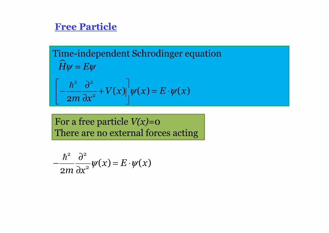
Time-independent Schrodinger equation
Free Particle
�H Eψ ψ=
V x x E xm x
2 2
2( ) ( ) ( )
2ψ ψ
∂− + = ⋅
∂
�
For a free particle V(x)=0There are no external forces acting
x E xm x
2 2
2( ) ( )
2ψ ψ
∂− = ⋅
∂
�
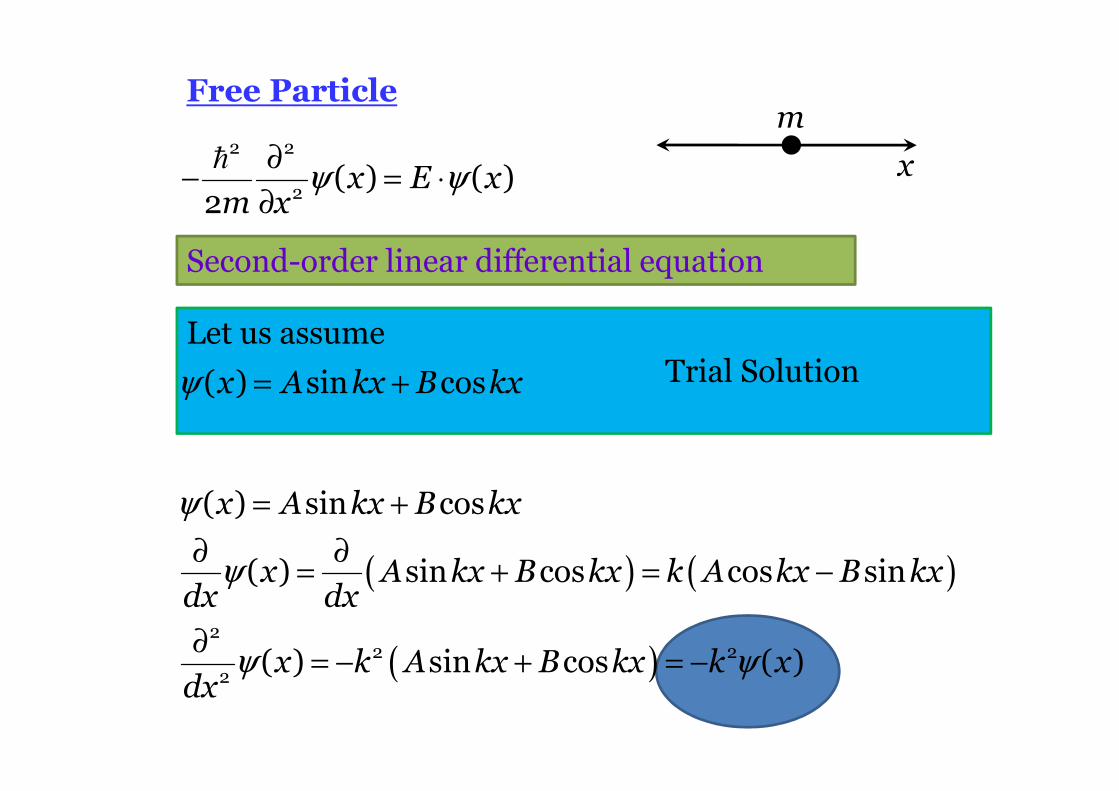
Free Particle
( ) ( )
( )
x A kx B kx
x A kx B kx k A kx B kxdx dx
x k A kx B kx k xdx
22 2
2
( ) sin cos
( ) sin cos cos sin
( ) sin cos ( )
ψ
ψ
ψ ψ
= +
∂ ∂= + = −
∂= − + = −
x E xm x
2 2
2( ) ( )
2ψ ψ
∂− = ⋅
∂
�
m
x
Second-order linear differential equation
Let us assumeTrial Solutionx A kx B kx( ) sin cosψ = +
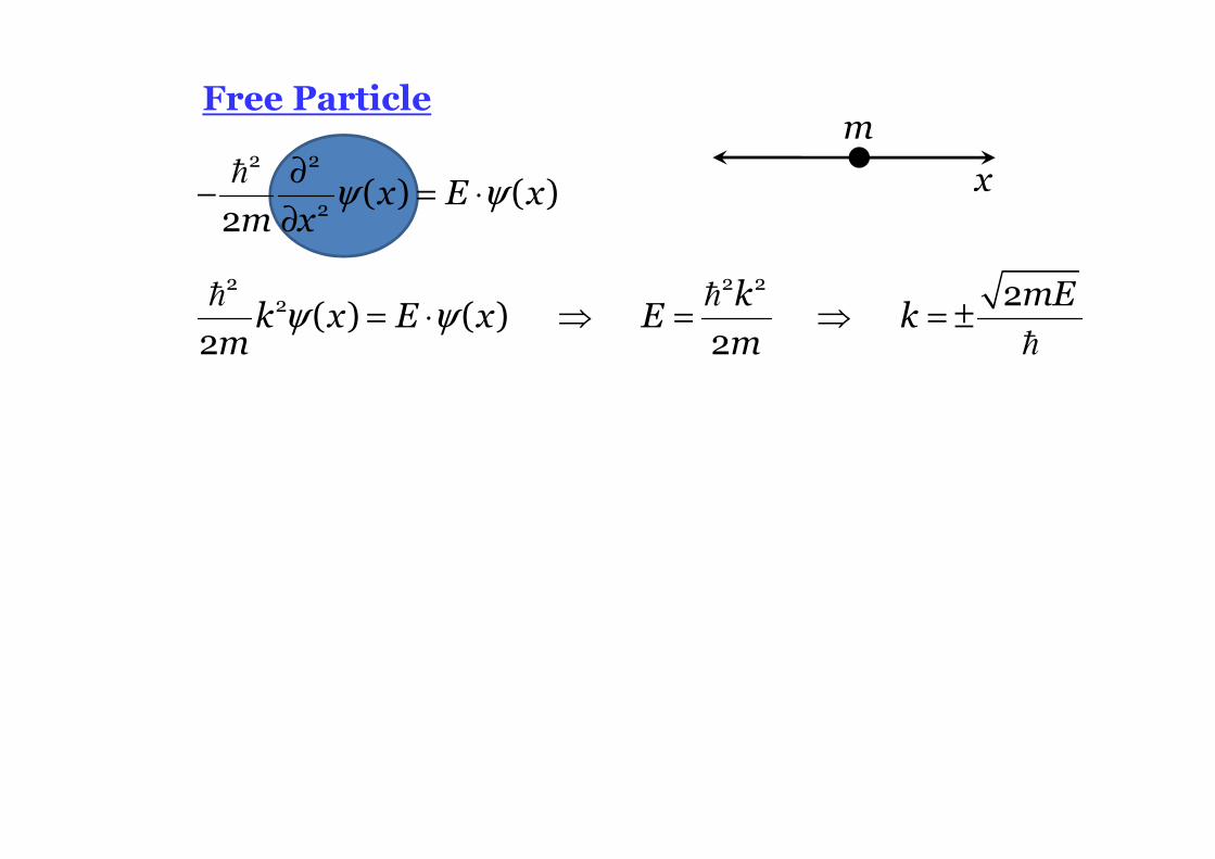
Free Particle
x E xm x
2 2
2( ) ( )
2ψ ψ
∂− = ⋅
∂
�
k mEk x E x E k
m m
2 2 22 2( ) ( )
2 2ψ ψ= ⋅ ⇒ = ⇒ = ±
� �
�
m
x
There are no restrictions on kE can have any valueEnergies of free particles are continuous
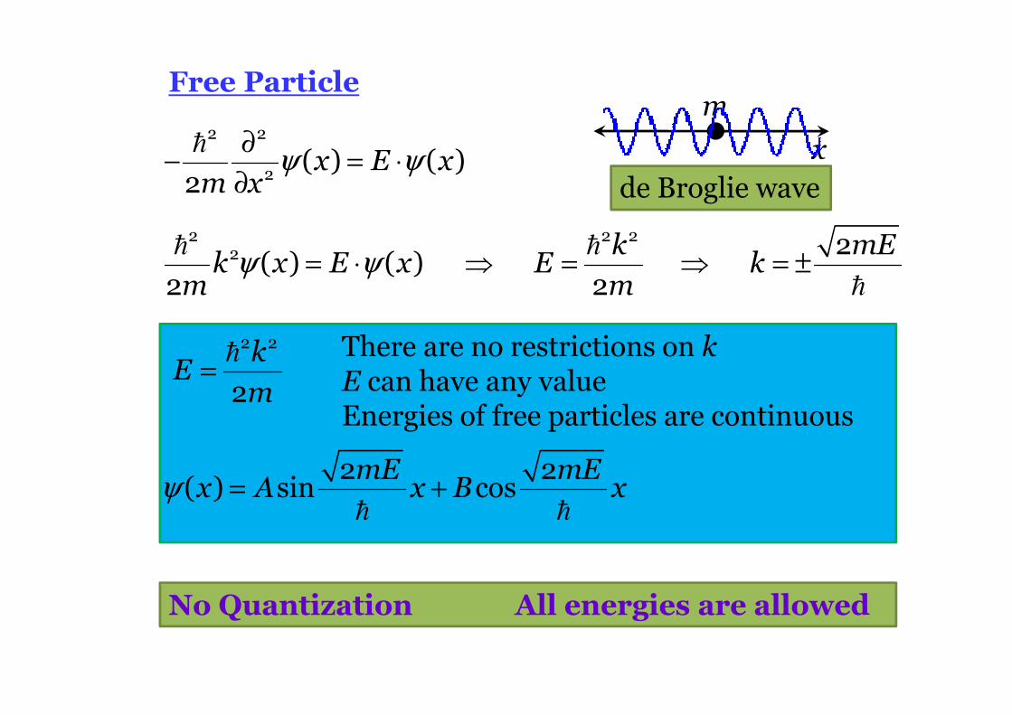
Free Particle
x E xm x
2 2
2( ) ( )
2ψ ψ
∂− = ⋅
∂
�
k mEk x E x E k
m m
2 2 22 2( ) ( )
2 2ψ ψ= ⋅ ⇒ = ⇒ = ±
� �
�
mE mEx A x B x
2 2( ) sin cosψ = +
� �
kE
m
2 2
2
=�
No Quantization All energies are allowed
m
xde Broglie wave
x
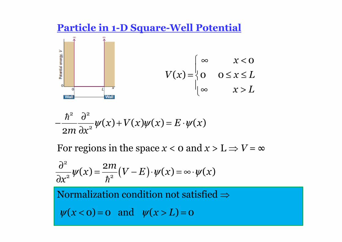
V x x L
x L
0
( ) 0 0
∞ <
= ≤ ≤∞ >
x V x x E xm x
2 2
2( ) ( ) ( ) ( )
2ψ ψ ψ
∂− + = ⋅
∂
�
For regions in the space x < 0 and x > L ⇒ V = ∞
( )m
x V E x xx
2
2 2
2( ) ( ) ( )ψ ψ ψ
∂= − ⋅ = ∞ ⋅
∂ �
Normalization condition not satisfied ⇒
x x L( 0) 0 and ( ) 0ψ ψ< = > =
Particle in 1-D Square-Well Potential
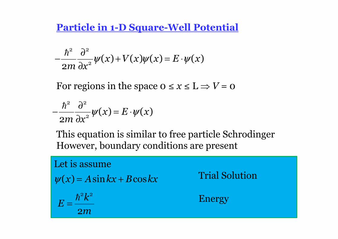
x V x x E xm x
2 2
2( ) ( ) ( ) ( )
2ψ ψ ψ
∂− + = ⋅
∂
�
For regions in the space 0 ≤ x ≤ L ⇒ V = 0
x E xm x
2 2
2( ) ( )
2ψ ψ
∂− = ⋅
∂
�
This equation is similar to free particle SchrodingerHowever, boundary conditions are present
Let is assumeTrial Solution
Energy
x A kx B kx( ) sin cosψ = +
kE
m
2 2
2
=�
Particle in 1-D Square-Well Potential
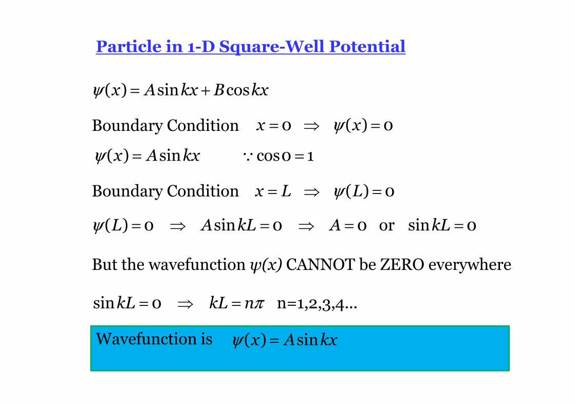
x A kx B kx( ) sin cosψ = +
Boundary Condition x x0 ( ) 0ψ= ⇒ =
Boundary Condition
x A kx( ) sin cos0 1ψ = =∵
x L L ( ) 0ψ= ⇒ =
L A kL A kL( ) 0 sin 0 0 or sin 0ψ = ⇒ = ⇒ = =
But the wavefunction ψ(x) CANNOT be ZERO everywhere
kL kL nsin 0 n=1,2,3,4...π= ⇒ =
Wavefunction is x A kx( ) sinψ =
Particle in 1-D Square-Well Potential
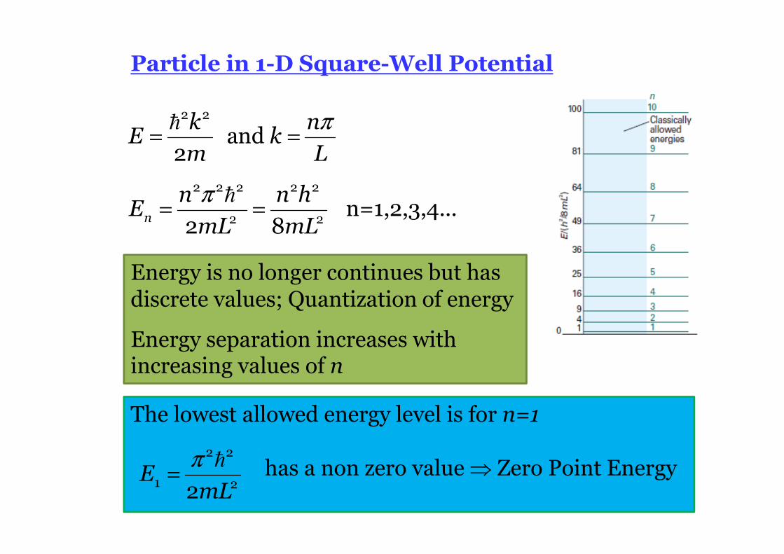
k nE k
m L
2 2
and 2
π= =�
n
n n hE
mL mL
2 2 2 2 2
2 2 n=1,2,3,4...
2 8π
= =�
Energy is no longer continues but has discrete values; Quantization of energy
Energy separation increases with increasing values of n
The lowest allowed energy level is for n=1
has a non zero value ⇒ Zero Point EnergyEmL
2 2
1 22π
=�
Particle in 1-D Square-Well Potential
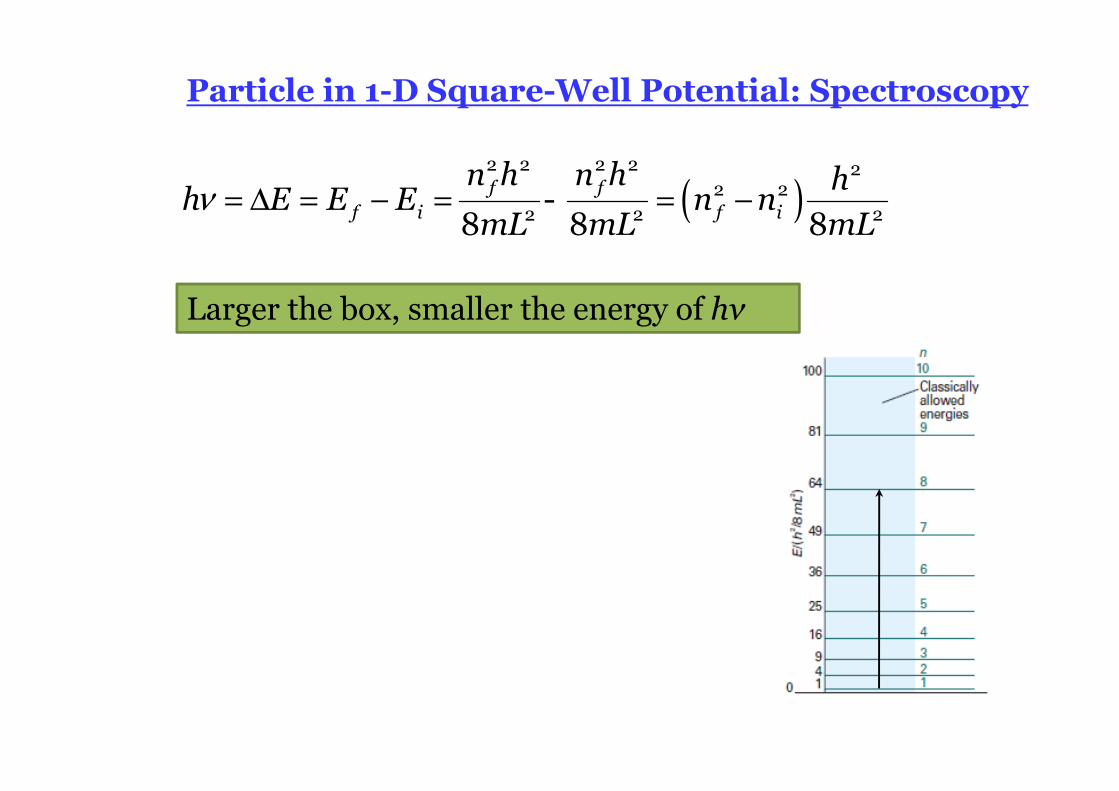
( )f ff i f i
n h n h hh E E E n n
mL mL mL
2 2 2 2 22 2
2 2 2-
8 8 8ν = ∆ = − = = −
Larger the box, smaller the energy of hν
Particle in 1-D Square-Well Potential: Spectroscopy
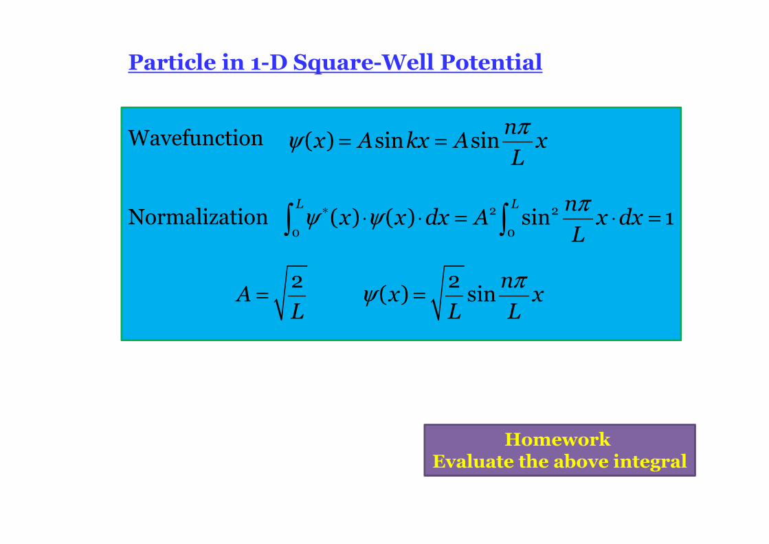
Wavefunction
Normalization
nx A kx A x
L( ) sin sin
πψ = =
L L nx x dx A x dx
L2 2
0 0( ) ( ) sin 1
πψ ψ∗ ⋅ ⋅ = ⋅ =∫ ∫
nA x x
L L L
2 2 ( ) sin
πψ= =
Homework Evaluate the above integral
Particle in 1-D Square-Well Potential
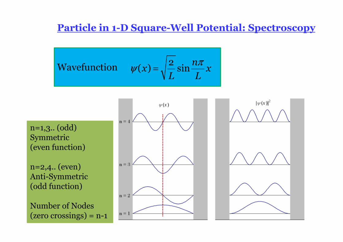
Wavefunction nx x
L L
2( ) sin
πψ =
n=1,3.. (odd) Symmetric(even function)
n=2,4.. (even) Anti-Symmetric(odd function)
Number of Nodes (zero crossings) = n-1
Particle in 1-D Square-Well Potential: Spectroscopy
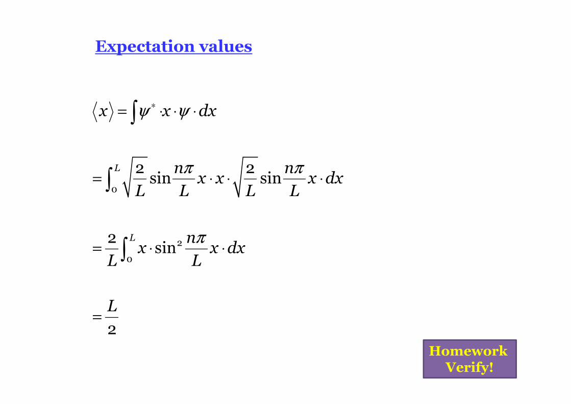
Expectation values
ψ ψ
π π
π
∗= ⋅ ⋅ ⋅
= ⋅ ⋅ ⋅
= ⋅ ⋅
=
∫
∫
∫
0
2
0
2 2sin sin
2sin
2
L
L
x x dx
n nx x x dx
L L L L
nx x dx
L L
L
Homework Verify!
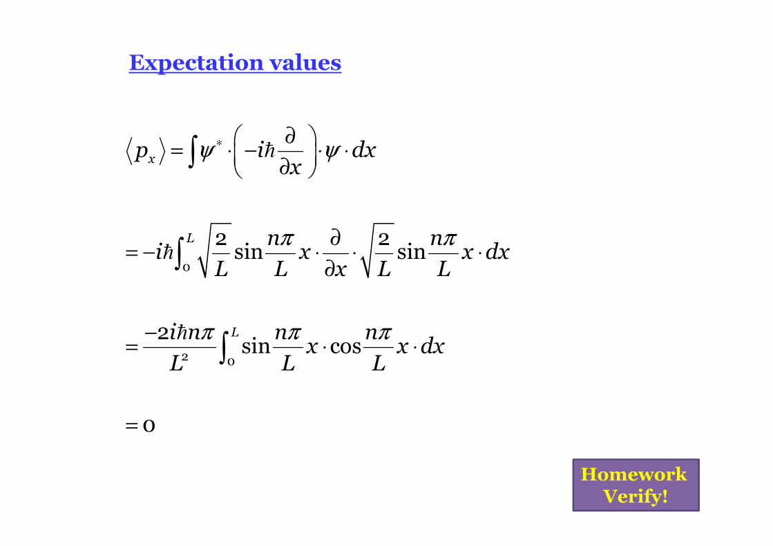
Expectation values
Homework Verify!
ψ ψ
π π
π π π
∗ ∂ = ⋅ − ⋅ ⋅
∂
∂= − ⋅ ⋅ ⋅
∂
−= ⋅ ⋅
=
∫
∫
∫
�
�
�
0
2 0
2 2sin sin
2sin cos
0
x
L
L
p i dxx
n ni x x dx
L L x L L
i n n nx x dx
L L L
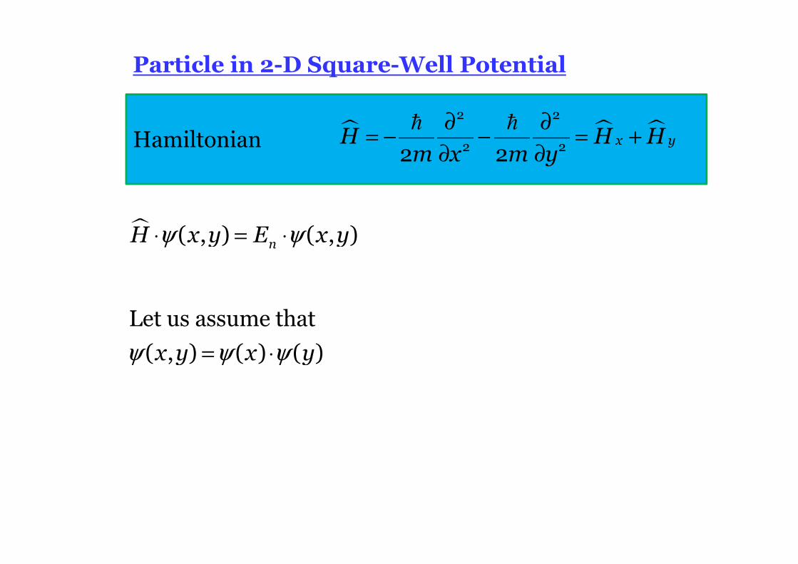
Hamiltonian � � �∂ ∂= − − = +
∂ ∂
� �2 2
2 22 2x yH H H
m x m y
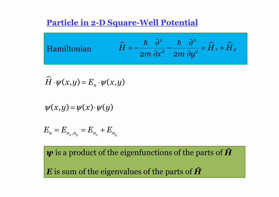
� ψ ψ⋅ = ⋅( , ) ( , )nH x y E x y
ψ ψ ψ= ⋅
Let us assume that
( , ) ( ) ( )x y x y
Particle in 2-D Square-Well Potential
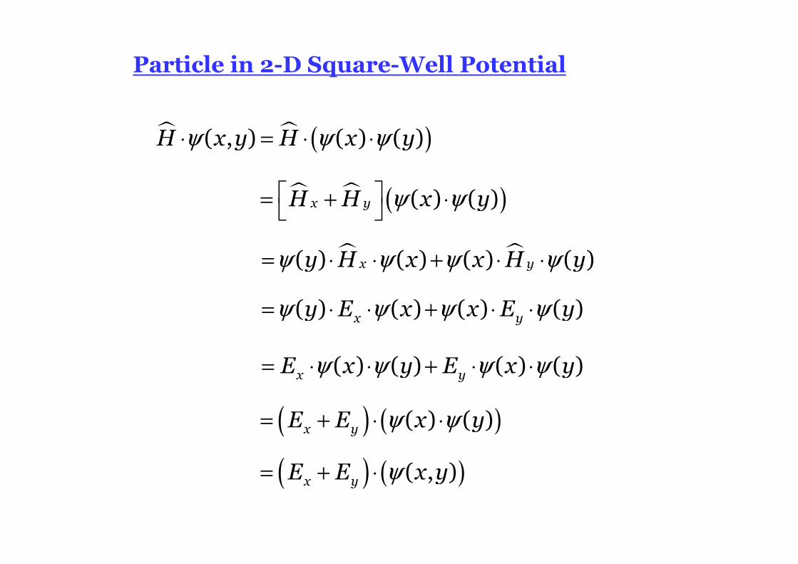
� � ( )H x y H x y( , ) ( ) ( )ψ ψ ψ⋅ = ⋅ ⋅
( ) ( )x yE E x y( , )ψ= + ⋅
� � ( )x yH H x y( ) ( )ψ ψ = + ⋅
� �x yy H x x H y( ) ( ) ( ) ( )ψ ψ ψ ψ= ⋅ ⋅ + ⋅ ⋅
x yy E x x E y( ) ( ) ( ) ( )ψ ψ ψ ψ= ⋅ ⋅ + ⋅ ⋅
x yE x y E x y( ) ( ) ( ) ( )ψ ψ ψ ψ= ⋅ ⋅ + ⋅ ⋅
( ) ( )x yE E x y( ) ( )ψ ψ= + ⋅ ⋅
Particle in 2-D Square-Well Potential
Hamiltonian � � �∂ ∂= − − = +
∂ ∂
� �2 2
2 22 2x yH H H
m x m y
ψ is a product of the eigenfunctions of the parts of Ĥ
E is sum of the eigenvalues of the parts of Ĥ
� ψ ψ⋅ = ⋅( , ) ( , )nH x y E x y
ψ ψ ψ= ⋅( , ) ( ) ( )x y x y
x y x yn n n n nE E E E,= = +
Particle in 2-D Square-Well Potential
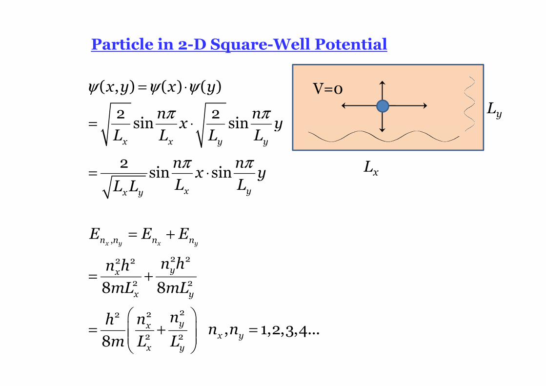
x y x yn n n n
yx
x y
yxx y
x y
E E E
n hn h
mL mL
nnhn n
m L L
,
2 22 2
2 2
222
2 2
8 8
, 1,2,3,4...8
= +
= +
= + =
x x y y
x yx y
x y x y
n nx y
L L L L
n nx y
L LL L
( , ) ( ) ( )
2 2sin sin
2sin sin
ψ ψ ψ
π π
π π
= ⋅
= ⋅
= ⋅
V=0
Lx
Ly
Particle in 2-D Square-Well Potential
( )
x y x yn n n n
yx
x y x y
E E E
n hn h
mL mL
hn n n n
mL
,
2 22 2
2 2
22 2
2
8 8
, 1,2,3,4...8
= +
= +
= + =
x y x y
n nx y
L L L Ln nx y
L L L
( , ) ( ) ( )
2 2sin sin
2sin sin
ψ ψ ψ
π π
π π
= ⋅
= ⋅
= ⋅
V=0
Lx
Ly
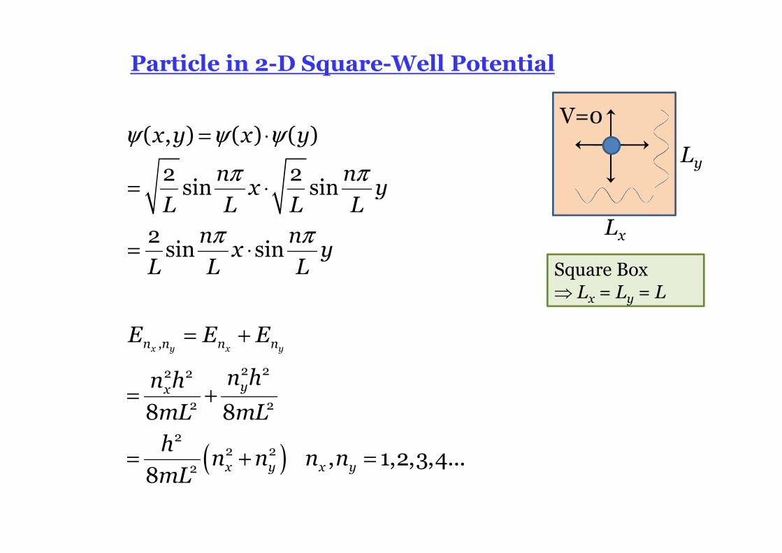
Square Box ⇒ Lx = Ly = L
Particle in 2-D Square-Well Potential
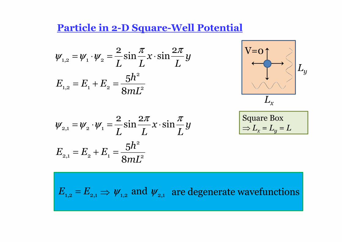
x yL L Lh
E E EmL
1,2 1 2
2
1,2 1 2 2
2 2sin sin
5
8
π πψ ψ ψ= ⋅ = ⋅
= + =
V=0
Lx
Ly
x yL L Lh
E E EmL
2,1 2 1
2
2,1 2 1 2
2 2sin sin
5
8
π πψ ψ ψ= ⋅ = ⋅
= + =
⇒ are degenerate wavefunctionsE E1,2 2,1= 1,2 2,1 and ψ ψ
Particle in 2-D Square-Well Potential
Square Box ⇒ Lx = Ly = L
V=0
Lx
Ly
V=0
Lx
Ly
(1,1)(2,1) (1,2)
(2,2)
(3,1) (1,3)
(1,1) (2,1)(3,1)
(1,2)(2,2)
(3,2)
(1,3)
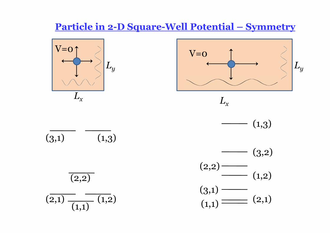
Particle in 2-D Square-Well Potential – Symmetry
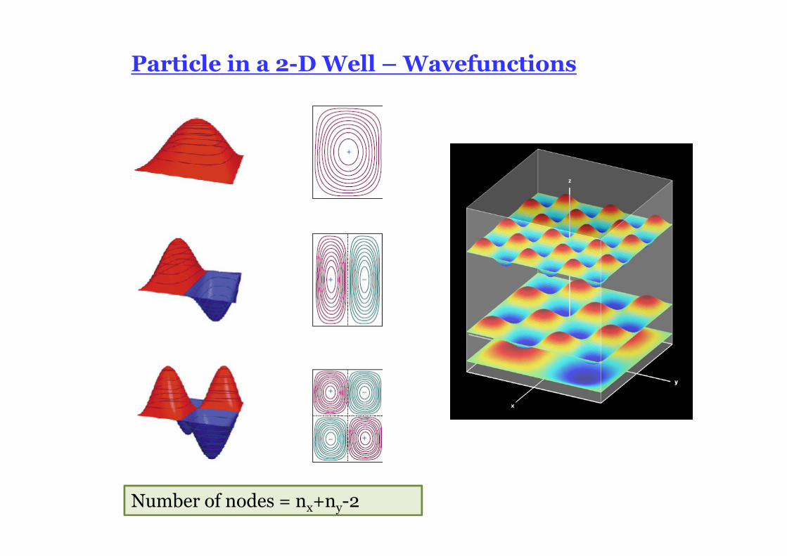
Number of nodes = nx+ny-2
Particle in a 2-D Well – Wavefunctions

Particle in a 3D-Box
yx z
x x y y z z
x y z x y z
nn nx y z
L L L L L L
( , , ) ( ) ( ) ( )
2 2 2sin sin sin
ψ ψ ψ ψ
ππ π
= ⋅ ⋅
= ⋅ ⋅
x y z x y zn n n n n n
yx zx y z
x y z
E E E E
n hn h n hn n n
mL mL mL
, ,
2 22 2 2 2
2 2 2 , , 1,2,3,4...
8 8 8
= + +
= + + =
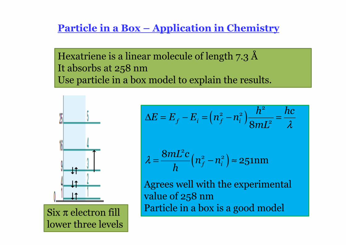
Agrees well with the experimental value of 258 nmParticle in a box is a good model
Particle in a Box – Application in Chemistry
Hexatriene is a linear molecule of length 7.3 ÅIt absorbs at 258 nmUse particle in a box model to explain the results.
�
�
�
Six π electron fill lower three levels
( )
( )
λ
λ
∆ = − = − =
= − ≈
22 2
2
22 2
8
8251nm
f i f i
f i
h hcE E E n n
mL
mL cn n
h
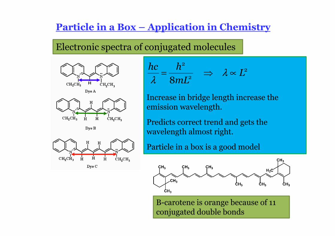
Increase in bridge length increase the emission wavelength.
Predicts correct trend and gets the wavelength almost right.
Particle in a box is a good model
Particle in a Box – Application in Chemistry
Electronic spectra of conjugated molecules
λλ
= ⇒ ∝2
22
8
hc hL
mL
Β-carotene is orange because of 11 conjugated double bonds
Particle in a Box – Application in nano-science
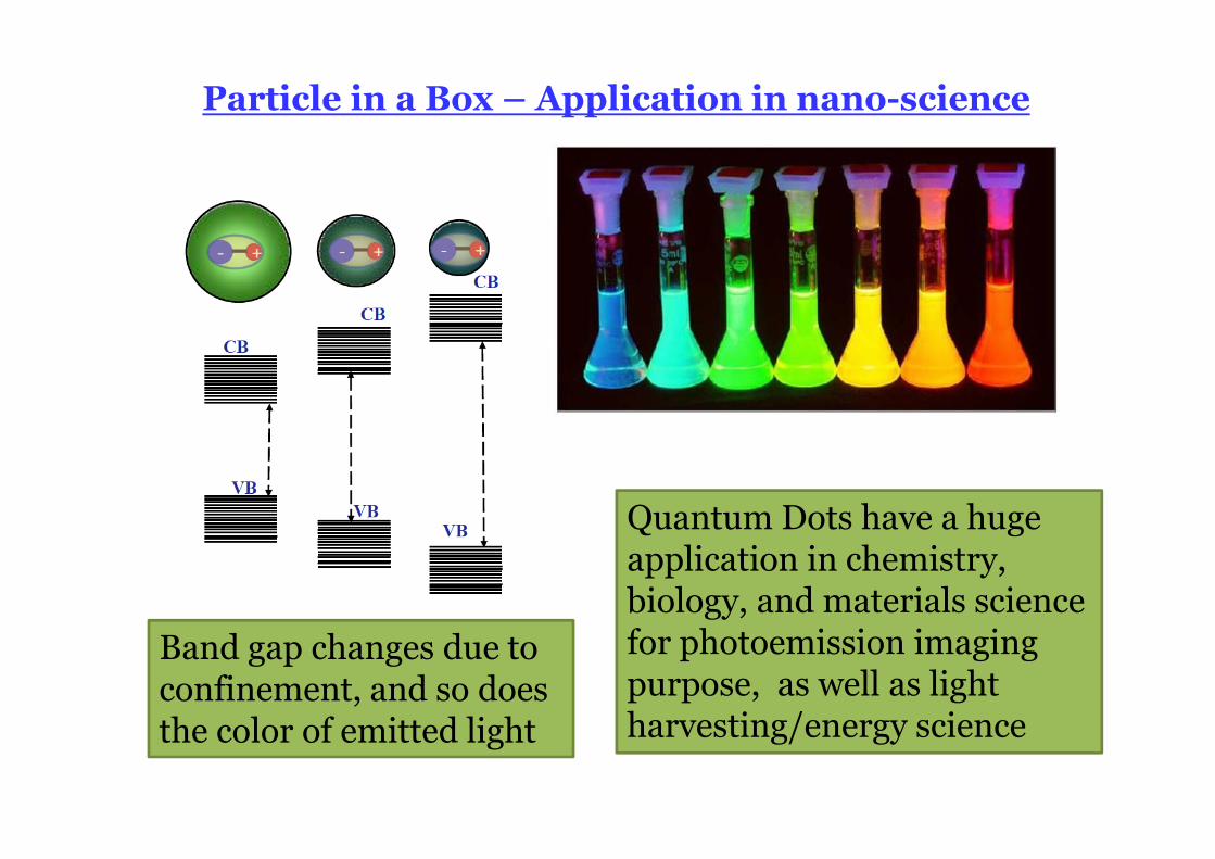
Band gap changes due to confinement, and so does the color of emitted light
Quantum Dots have a huge application in chemistry, biology, and materials sciencefor photoemission imaging purpose, as well as light harvesting/energy science
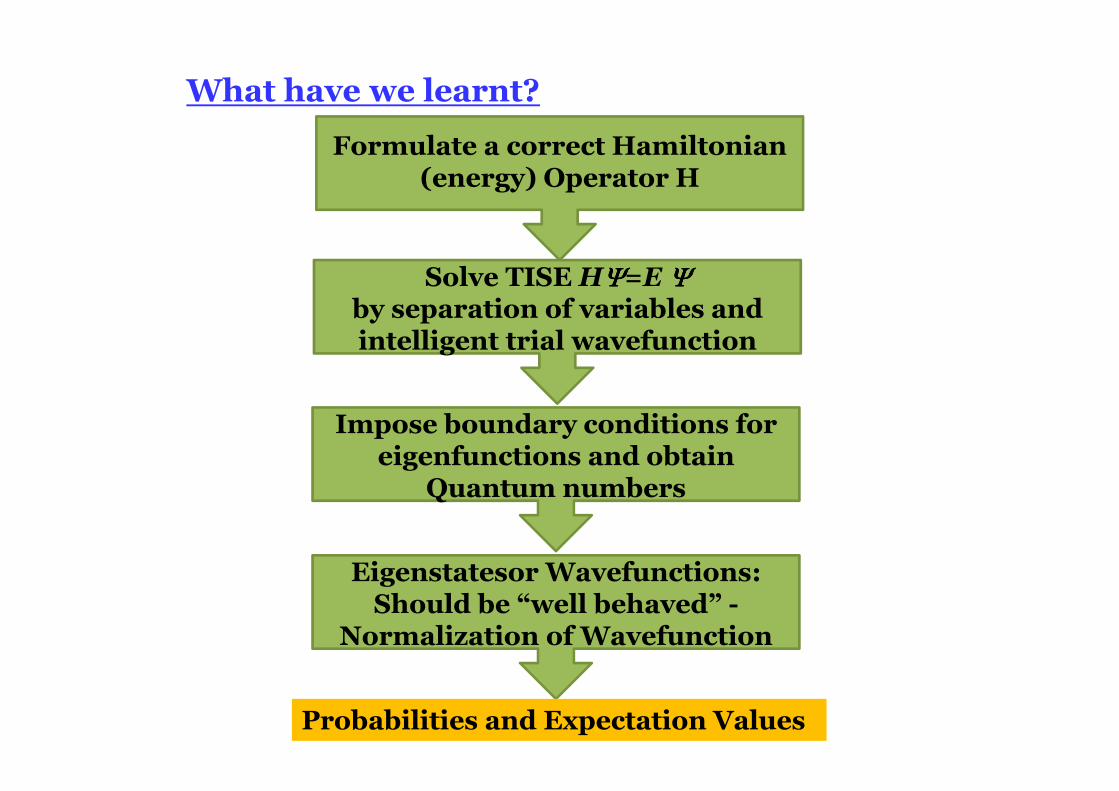
What have we learnt?
Formulate a correct Hamiltonian(energy) Operator H
Solve TISE HΨΨΨΨ=E ΨΨΨΨby separation of variables and intelligent trial wavefunction
Impose boundary conditions for eigenfunctions and obtain
Quantum numbers
Eigenstatesor Wavefunctions: Should be “well behaved” -
Normalization of Wavefunction
Probabilities and Expectation Values
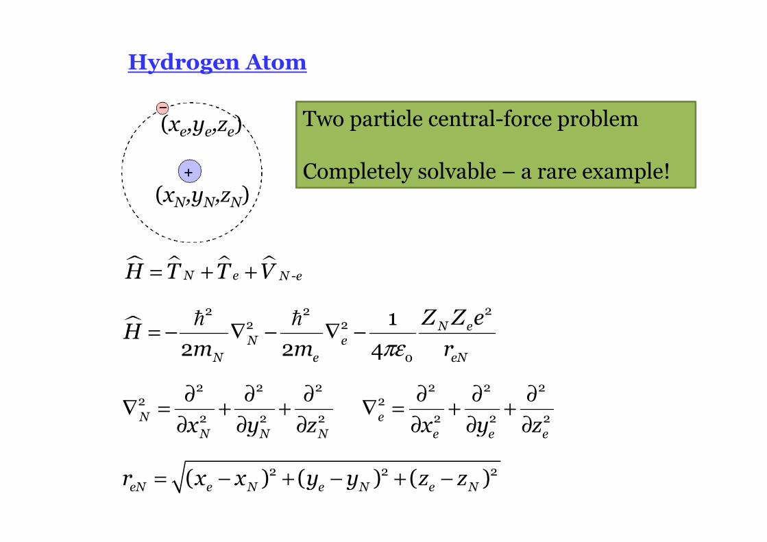
Hydrogen Atom
�
πε= − ∇ − ∇ −
� �22 2
2 2
0
1
2 2 4N e
N eN e eN
Z Z eH
m m r
� � � �N e N eH T T V -= + +
(xe,ye,ze)
= − + − + −2 2 2( ) ( ) ( )eN e N e N e Nr x x y y z z
(xN,yN,zN)
N eN N N e e ex y z x y z
2 2 2 2 2 22 2
2 2 2 2 2 2
∂ ∂ ∂ ∂ ∂ ∂∇ = + + ∇ = + +
∂ ∂ ∂ ∂ ∂ ∂
Two particle central-force problem
Completely solvable – a rare example!
Hydrogen Atom
− ∇ − ∇ − Ψ = ⋅Ψ
� �2 2 2
2 2
2 2N e Total Total TotalN e eN
QZeE
m m r
Schrodinger Equation
Total N N N e e ex y z x y z( , , , , , )Ψ = Ψ
�
πε= − ∇ − ∇ −
� �22 2
2 2
0
1
2 2 4N e
N eN e eN
Z Z eH
m m r
�
πε
= − ∇ − ∇ −
= = =
� �2 2 2
2 2
0
2 2
1 with 1 and
4
N eN e eN
N e
QZeH
m m r
Z Z Z Q
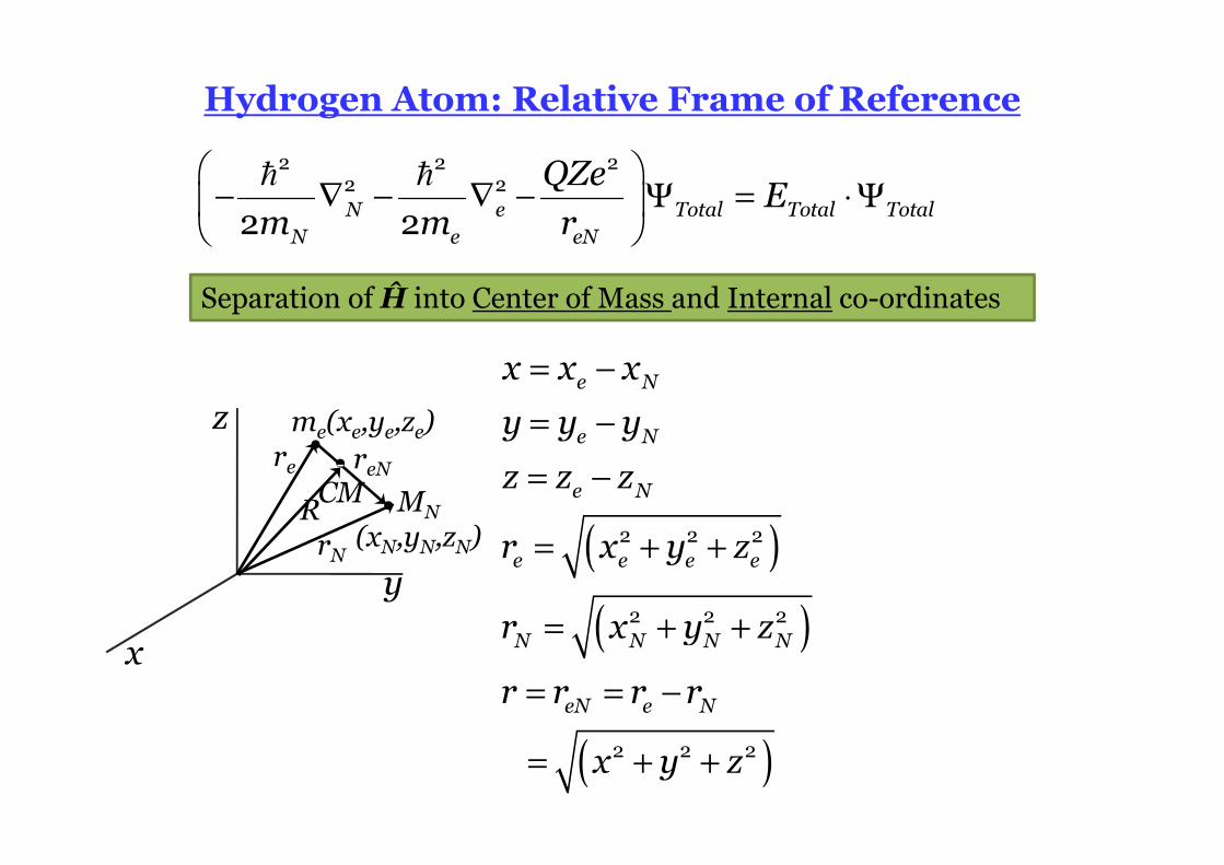
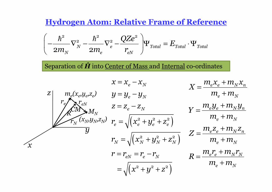
Hydrogen Atom: Relative Frame of Reference
Separation of Ĥ into Center of Mass and Internal co-ordinates
x
z
y
-re
RrN
me(xe,ye,ze)
CMreNMN
(xN,yN,zN) ( )
( )
( )
= −
= −
= −
= + +
= + +
= = −
= + +
2 2 2
2 2 2
2 2 2
e N
e N
e N
e e e e
N N N N
eN e N
x x x
y y y
z z z
r x y z
r x y z
r r r r
x y z
− ∇ − ∇ − Ψ = ⋅Ψ
� �2 2 2
2 2
2 2N e Total Total TotalN e eN
QZeE
m m r
Hydrogen Atom: Relative Frame of Reference
Separation of Ĥ into Center of Mass and Internal co-ordinates
x
z
y
-re
RrN
me(xe,ye,ze)
CMreNMN
(xN,yN,zN)
+=
+
+=
+
+=
+
+=
+
e e N n
e N
e e N n
e N
e e N n
e N
e e N N
e N
m x m xX
m m
m y m yY
m m
m z m zZ
m m
m r m rR
m m
− ∇ − ∇ − Ψ = ⋅Ψ
� �2 2 2
2 2
2 2N e Total Total TotalN e eN
QZeE
m m r
( )
( )
( )
= −
= −
= −
= + +
= + +
= = −
= + +
2 2 2
2 2 2
2 2 2
e N
e N
e N
e e e e
N N N N
eN e N
x x x
y y y
z z z
r x y z
r x y z
r r r r
x y z
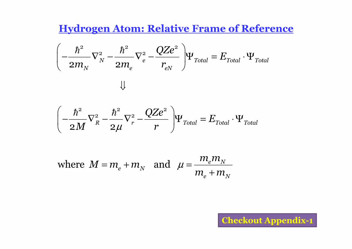
Hydrogen Atom: Relative Frame of Reference
µ
µ
− ∇ − ∇ − Ψ = ⋅Ψ
= + =+
� �2 2 2
2 2
2 2
where and
R r Total Total Total
e Ne N
e N
QZeE
M r
m mM m m
m m
⇓
− ∇ − ∇ − Ψ = ⋅Ψ
� �2 2 2
2 2
2 2N e Total Total TotalN e eN
QZeE
m m r
Checkout Appendix-1
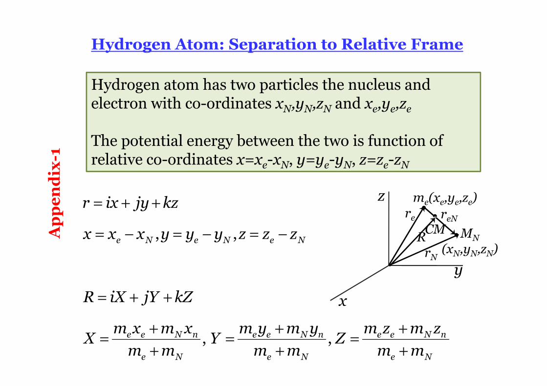
Hydrogen Atom: Separation to Relative Frame
Hydrogen atom has two particles the nucleus and electron with co-ordinates xN,yN,zN and xe,ye,ze
The potential energy between the two is function of relative co-ordinates x=xe-xN, y=ye-yN, z=ze-zN
= + +
= − = − = −
= + +
+ + += = =
+ + +
, ,
, ,
e N e N e N
e e N n e e N n e e N n
e N e N e N
r ix jy kz
x x x y y y z z z
R iX jY kZ
m x m x m y m y m z m zX Y Z
m m m m m m
x
z
y
-re
RrN
me(xe,ye,ze)
CMreNMN
(xN,yN,zN)
Appendix-1
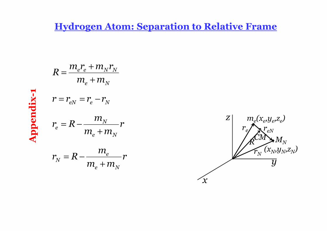
+=
+
= = −
= −+
= −+
e e N N
e N
eN e N
Ne
e N
eN
e N
m r m rR
m m
r r r r
mr R r
m m
mr R r
m m
Hydrogen Atom: Separation to Relative Frame
x
z
y
-re
RrN
me(xe,ye,ze)
CMreNMN
(xN,yN,zN)
Appendix-1
( )
µ µ
= +
= − ⋅ −
+ +
+ − ⋅ −
+ +
= + +
+
= + = + =+
� �
� �� �
� �� �
� �
� �
2 2
2 2
2 2
1 1
2 2
1
2
1
2
1 1
2 2
1 1 where and
2 2
e e N N
N Ne
e N e N
e ee
e N e N
e Ne N
e N
e Ne N
e N
T m r m r
m mT m R r R r
m m m m
m mm R r R r
m m m m
m mT m m R r
m m
m mT M R r M m m
m m
Hydrogen Atom: Separation to Relative Frame
=
=
=
=
�
�
�
�
ee
NN
drr
dtdr
rdtdr
rdtdR
Rdt
Appendix-1
µ
µ
= +
= +
� �2 2
2 2
1 1
2 2
2 2R r
T M R r
p pT
M
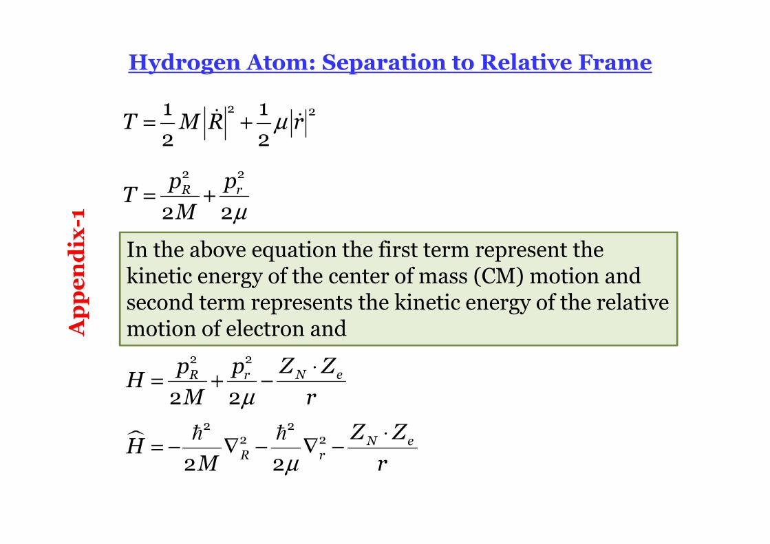
Hydrogen Atom: Separation to Relative Frame
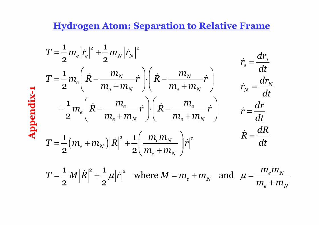
In the above equation the first term represent the kinetic energy of the center of mass (CM) motion and second term represents the kinetic energy of the relative motion of electron and
�
µ
µ
⋅= + −
⋅= − ∇ − ∇ −� �
2 2
2 22 2
2 2
2 2
N eR r
N eR r
Z Zp pH
M r
Z ZH
M r
Appendix-1
Free particle!Kinetic energy of the atom
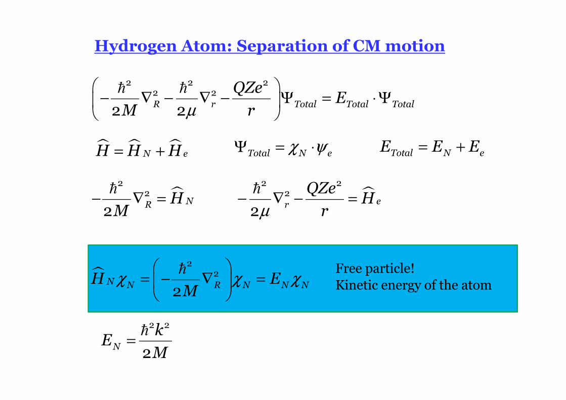
Hydrogen Atom: Separation of CM motion
� χ χ χ
= − ∇ =
�2
2
2N N R N N NH E
M
=�2 2
2N
kE
M
χ ψΨ = ⋅Total N e� � �= +N eH H H = +Total N eE E E
µ
− ∇ − ∇ − Ψ = ⋅Ψ
� �2 2 2
2 2
2 2R r Total Total Total
QZeE
M r
� �
µ− ∇ = − ∇ − =� �2 2 2
2 2 2 2
N eR r
QZeH H
M r
Hydrogen Atom: Electronic Hamiltonian
( )ψ ψ
µ
ψ
∂ ∂ ∂− + + −
∂ ∂ ∂ + +
= ⋅
�2 2 2 2 2
2 2 2 2 2 2( , , ) ( , , )
2
( , , )
e e
e e
QZex y z x y z
x y z x y z
E x y z
Not possible to separate out into three different co-ordinates. Need a new co-ordinate system
r
� ψ ψ ψµ
ψ ψ
⋅ = − ∇ − = ⋅
⇒
�2 2
2
2
( , , )
e e r e e e
e e
QZeH E
r
x y z
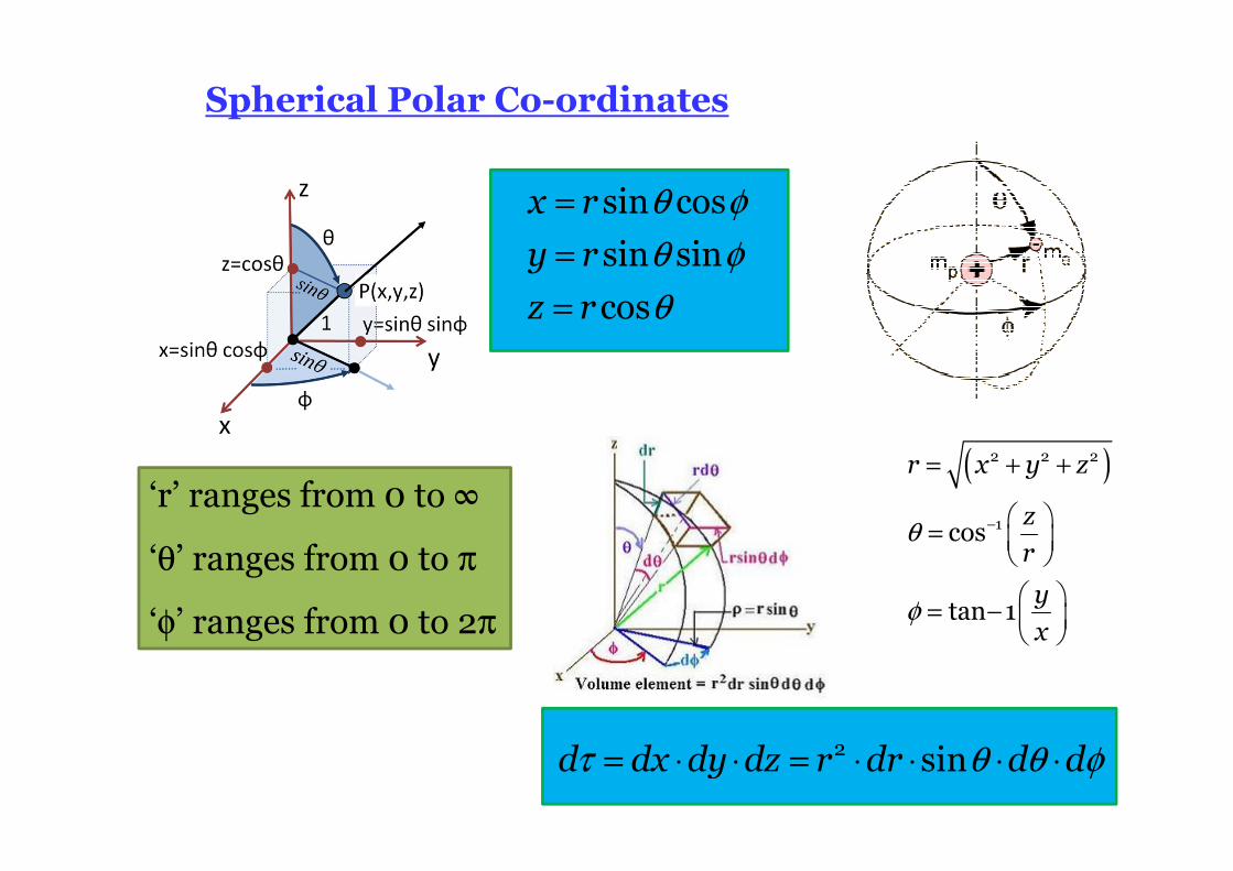
Spherical Polar Co-ordinates
θ φ
θ φ
θ
=
=
=
sin cos
sin sin
cos
x r
y r
z r
( )
θ
φ
−
= + +
=
= −
2 2 2
1cos
tan 1
r x y z
zr
y
x
τ θ θ φ= ⋅ ⋅ = ⋅ ⋅ ⋅ ⋅2 sind dx dy dz r dr d d
‘r’ ranges from 0 to ∞
‘θ’ ranges from 0 to π
‘φ’ ranges from 0 to 2π
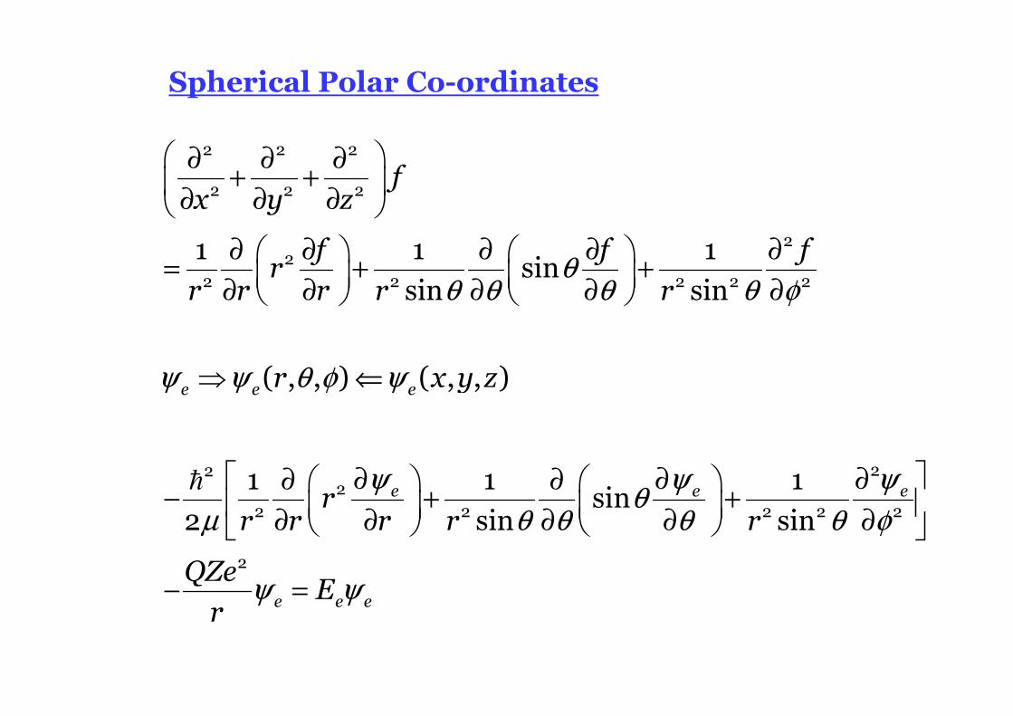
Spherical Polar Co-ordinates
ψ ψ θ φ ψ⇒ ⇐( , , ) ( , , )e e er x y z
θθ θ θ θ φ
∂ ∂ ∂+ +
∂ ∂ ∂
∂ ∂ ∂ ∂ ∂ = + +
∂ ∂ ∂ ∂ ∂
2 2 2
2 2 2
22
2 2 2 2 2
1 1 1sin
sin sin
fx y z
f f fr
r r r r r
ψ ψ ψθ
µ θ θ θ θ φ
ψ ψ
∂ ∂ ∂∂ ∂ − + + ∂ ∂ ∂ ∂ ∂
− =
�22
22 2 2 2 2
2
1 1 1sin
2 sin sine e e
e e e
rr r r r r
QZeE
r
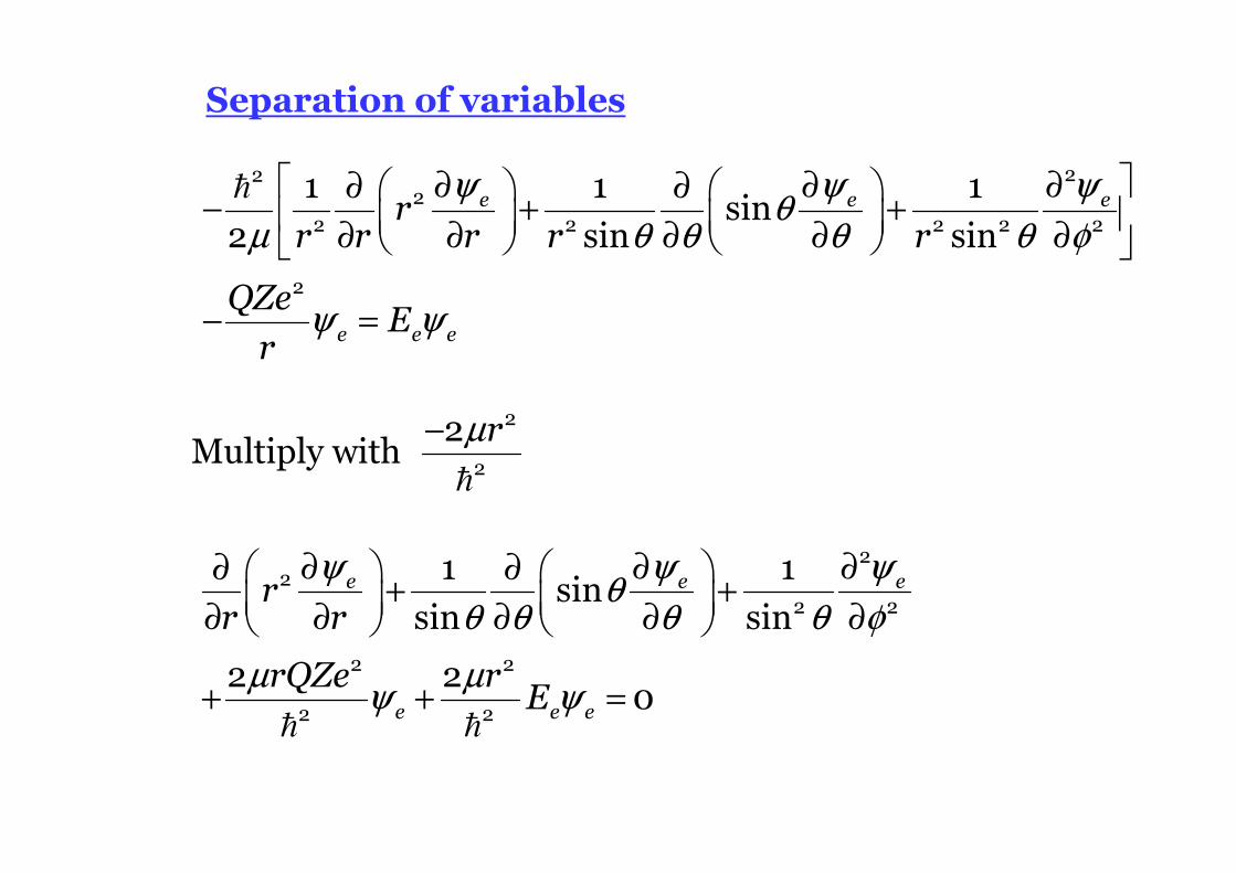
Separation of variables
ψ ψ ψθ
µ θ θ θ θ φ
ψ ψ
∂ ∂ ∂∂ ∂ − + + ∂ ∂ ∂ ∂ ∂
− =
�22
22 2 2 2 2
2
1 1 1sin
2 sin sine e e
e e e
rr r r r r
QZeE
r
µ−
�
2
2
2Multiply with
r
ψ ψ ψθ
θ θ θ θ φ
µ µψ ψ
∂ ∂ ∂∂ ∂ + + ∂ ∂ ∂ ∂ ∂
+ + =� �
22
2 2
2 2
2 2
1 1sin
sin sin
2 20
e e e
e e e
rr r
rQZe rE
Separation of variables
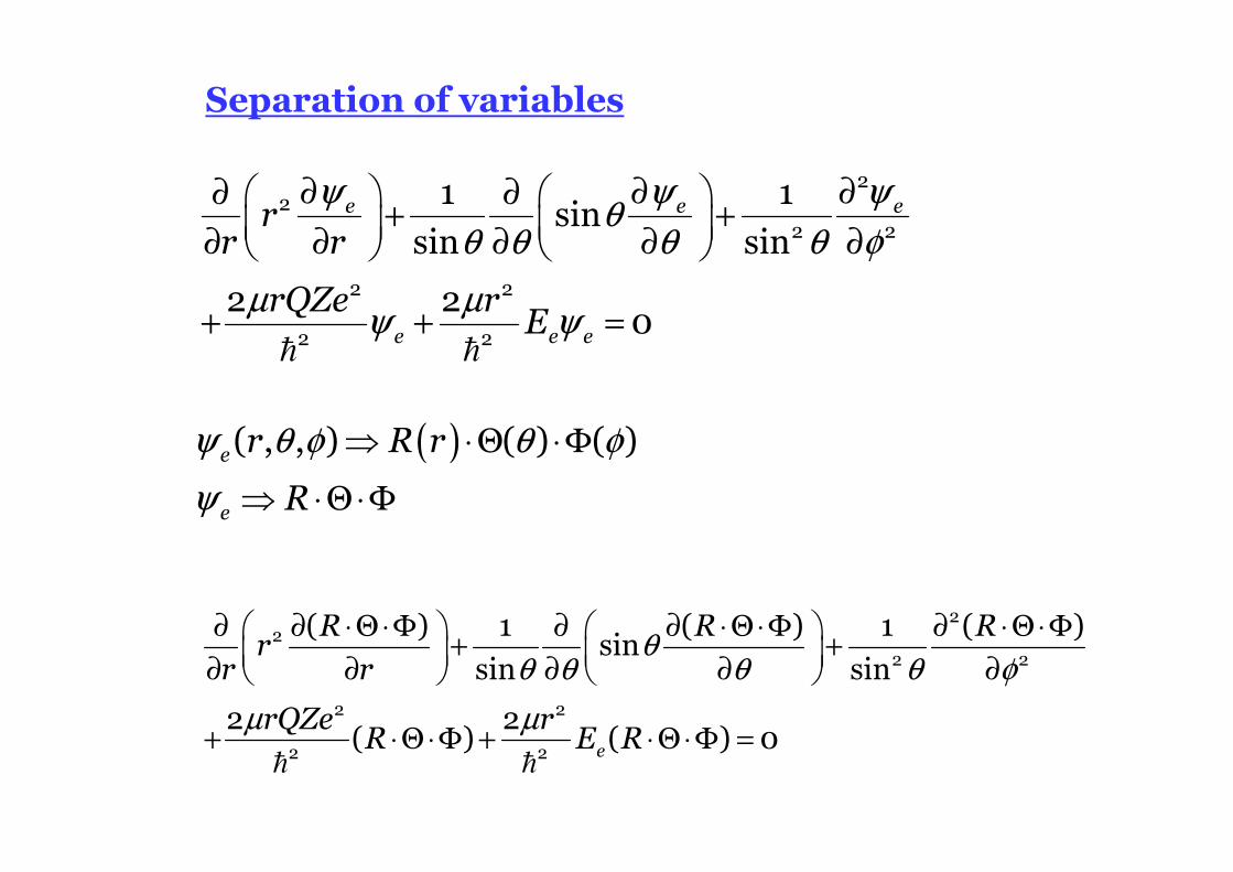
( )ψ θ φ θ φ
ψ
⇒ ⋅Θ ⋅Φ
⇒ ⋅Θ ⋅Φ
( , , ) ( ) ( )e
e
r R r
R
θθ θ θ θ φ
µ µ
∂ ∂ ⋅Θ⋅Φ ∂ ∂ ⋅Θ⋅Φ ∂ ⋅Θ⋅Φ + +
∂ ∂ ∂ ∂ ∂
+ ⋅Θ⋅Φ + ⋅Θ⋅Φ =� �
22
2 2
2 2
2 2
( ) 1 ( ) 1 ( )sin
sin sin
2 2( ) ( ) 0e
R R Rr
r r
rQZe rR E R
ψ ψ ψθ
θ θ θ θ φ
µ µψ ψ
∂ ∂ ∂∂ ∂ + + ∂ ∂ ∂ ∂ ∂
+ + =� �
22
2 2
2 2
2 2
1 1sin
sin sin
2 20
e e e
e e e
rr r
rQZe rE
Separation of variables
θθ θ θ θ φ
µ µ
∂ ∂ ⋅Θ⋅Φ ∂ ∂ ⋅Θ⋅Φ ∂ ⋅Θ⋅Φ + +
∂ ∂ ∂ ∂ ∂
+ ⋅Θ⋅Φ + ⋅Θ⋅Φ =� �
22
2 2
2 2
2 2
( ) 1 ( ) 1 ( )sin
sin sin
2 2( ) ( ) 0e
R R Rr
r r
rQZe rR E R
θθ θ θ θ φ
µ µ
∂ ∂ ∂ ∂Θ ∂ Φ Θ⋅Φ + ⋅Φ + ⋅Θ
∂ ∂ ∂ ∂ ∂
+ ⋅Θ⋅Φ + ⋅Θ⋅Φ =� �
22
2 2
2 2
2 2
1 1( ) ( ) sin ( )
sin sin
2 2( ) ( ) 0e
Rr R R
r r
rQZe rR E R
Rearrange
Separation of variables
∂ ∂ ∂ ∂Θ ∂ Φ Θ⋅Φ + ⋅Φ + ⋅Θ
∂ ∂ ∂ ∂ ∂
+ ⋅Θ⋅Φ + ⋅Θ⋅Φ =� �
22
2 2
2 2
2 2
1 1( ) ( ) sin ( )
sin sin
2 2( ) ( ) 0e
Rr R R
r r
rQZe rR E R
θθ θ θ θ φ
µ µ
⋅Θ ⋅Φ
1Multiply with
R
∂ ∂ ∂ ∂Θ ∂ Φ + +
∂ ∂ Θ ∂ ∂ Φ ∂
+ + =� �
22
2 2
2 2
2 2
1 1 1 1 1sin
sin sin
2 20e
Rr
R r r
rQZe rE
θθ θ θ θ φ
µ µ
Separation of variables
∂ ∂ ∂ ∂Θ ∂ Φ + +
∂ ∂ Θ ∂ ∂ Φ ∂
+ + =� �
22
2 2
2 2
2 2
1 1 1 1 1sin
sin sin
2 20e
Rr
R r r
rQZe rE
θθ θ θ θ φ
µ µ
Rearrange
∂ ∂ + + +
∂ ∂
∂ ∂Θ ∂ Φ = − +
Θ ∂ ∂ Φ ∂
� �
2 22
2 2
2
2 2
1 2 2
1 1 1 1sin
sin sin
e
R rQZe rr E
R r r
µ µ
θθ θ θ θ φ
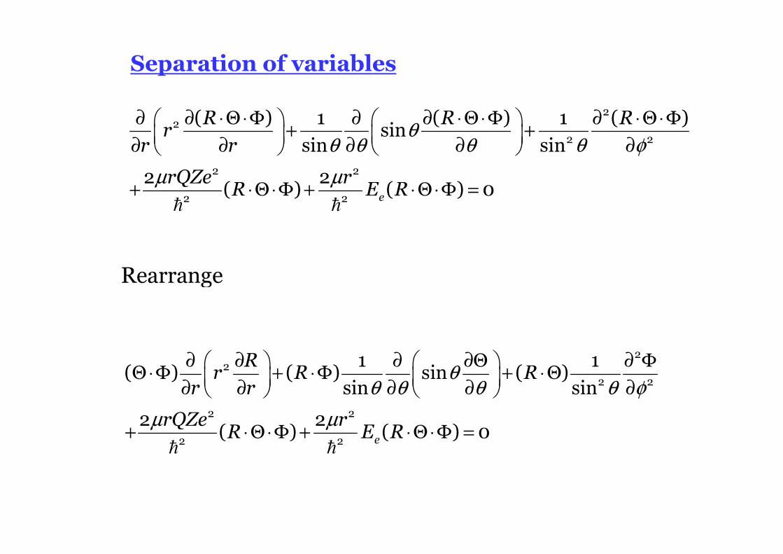
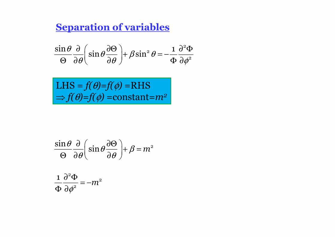
LHS = f(r)=f(θ ,φ) =RHS⇒ f(r)=f(θ ,φ) =constant=β

Separation of variables
∂ ∂ ∂ ∂Θ ∂ Φ + +
∂ ∂ Θ ∂ ∂ Φ ∂
+ + =� �
22
2 2
2 2
2 2
1 1 1 1 1sin
sin sin
2 20e
Rr
R r r
rQZe rE
θθ θ θ θ φ
µ µ
Rearrange
∂ ∂ + + +
∂ ∂
∂ ∂Θ ∂ Φ = − + =
Θ ∂ ∂ Φ ∂
� �
2 22
2 2
2
2 2
1 2 2
1 1 1 1sin
sin sin
e
R rQZe rr E
R r r
µ µ
θ βθ θ θ θ φ
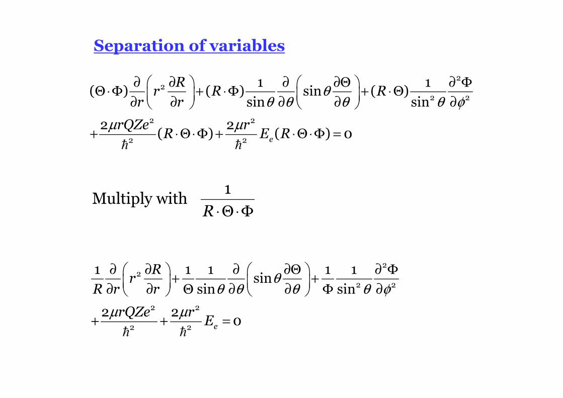
LHS = f(r)=f(θ ,φ) =RHS⇒ f(r)=f(θ ,φ) =constant=β
Separation of variables
∂ ∂ + + + =
∂ ∂
∂ ∂Θ ∂ Φ + = −
Θ ∂ ∂ Φ ∂
� �
2 22
2 2
2
2 2
1 2 2
1 1 1 1sin
sin sin
e
R rQZe rr E
R r rµ µ
β
θ βθ θ θ θ φ
θ βθ θ θ θ φ
∂ ∂Θ ∂ Φ + = −
Θ ∂ ∂ Φ ∂
2
2 2
1 1 1 1sin
sin sin
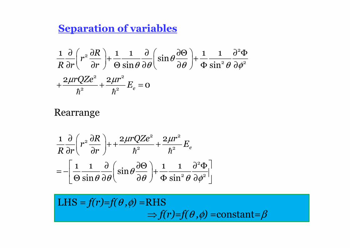
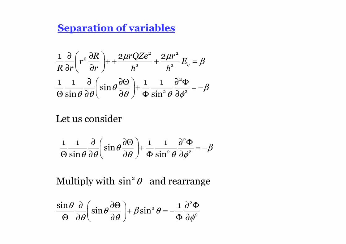
Let us consider
θ2Multiply with sin and rearrange
θθ β θ
θ θ φ
∂ ∂Θ ∂ Φ + = −
Θ ∂ ∂ Φ ∂
22
2
sin 1sin sin
θθ β
θ θ
∂ ∂Θ + =
Θ ∂ ∂
2sinsin m
φ
∂ Φ= −
Φ ∂
22
2
1m
Separation of variables
θθ β θ
θ θ φ
∂ ∂Θ ∂ Φ + = −
Θ ∂ ∂ Φ ∂
22
2
sin 1sin sin
LHS = f(θ)=f(φ) =RHS⇒ f(θ)=f(φ) =constant=m2
∂ ∂ + + + =
∂ ∂ � �
2 22
2 2
1 2 2e
R rQZe rr E
R r r
µ µβ
θθ β θ
θ θ
∂ ∂Θ + =
Θ ∂ ∂
2 2sinsin sin m
φ
∂ Φ= −
Φ ∂
22
2
1m
Separation of variables
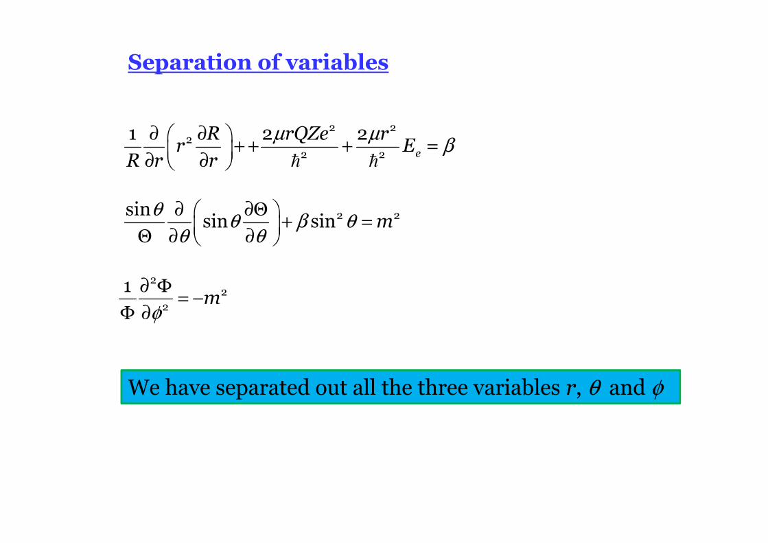
We have separated out all the three variables r, θ and φ
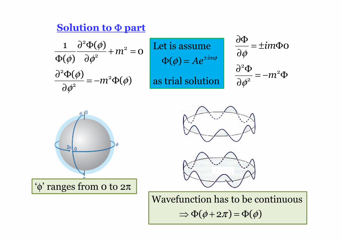
Solution to ΦΦΦΦ part
φ
φ φ
φφ
φ
∂ Φ+ =
Φ ∂
∂ Φ= − Φ
∂
22
2
22
2
1 ( )0
( )
( )( )
m
m
Let is assume
as trial solution
φφ ±Φ =( ) imAeφ
φ
∂Φ= ± Φ
∂
∂ Φ= − Φ
∂
22
2
0im
m
Wavefunction has to be continuous
φ π φ⇒ Φ + = Φ( 2 ) ( )
‘φ’ ranges from 0 to 2π
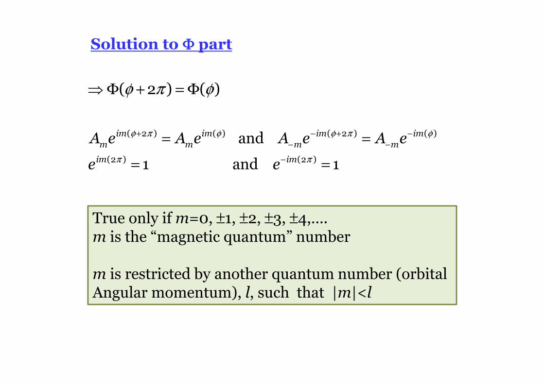
Solution to ΦΦΦΦ part
φ π φ φ π φ
π π
+ − + −
− −
−
= =
= =
( 2 ) ( ) ( 2 ) ( )
(2 ) (2 )
and
1 and 1
im im im imm m m m
im im
A e A e A e A e
e e
True only if m=0, ±1, ±2, ±3, ±4,….m is the “magnetic quantum” number
m is restricted by another quantum number (orbital Angular momentum), l, such that |m|<l
φ π φ⇒ Φ + = Φ( 2 ) ( )
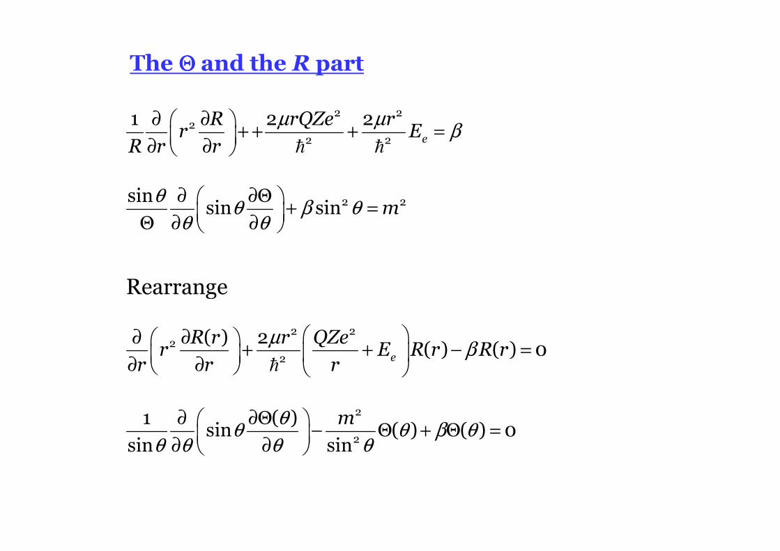
The ΘΘΘΘ and the R part
∂ ∂ + + + =
∂ ∂ � �
2 22
2 2
1 2 2e
R rQZe rr E
R r r
µ µβ
θθ β θ
θ θ
∂ ∂Θ + =
Θ ∂ ∂
2 2sinsin sin m
∂ ∂ + + − =
∂ ∂ �
2 22
2
( ) 2( ) ( ) 0e
R r r QZer E R r R r
r r rµ
β
θθ θ β θ
θ θ θ θ
∂ ∂Θ − Θ + Θ =
∂ ∂
2
2
1 ( )sin ( ) ( ) 0
sin sin
m
Rearrange
Solve to get Θ(θ)
Need serious mathematical skill to solve these two equations. We only look at solutions
The ΘΘΘΘ and the R part
∂ ∂ + + − =
∂ ∂ �
2 22
2
( ) 2( ) ( ) 0e
R r r QZer E R r R r
r r rµ
β
θθ θ β θ
θ θ θ θ
∂ ∂Θ − Θ + Θ =
∂ ∂
2
2
1 ( )sin ( ) ( ) 0
sin sin
m
Solve to get R(r)
Restriction on m are due this this equation
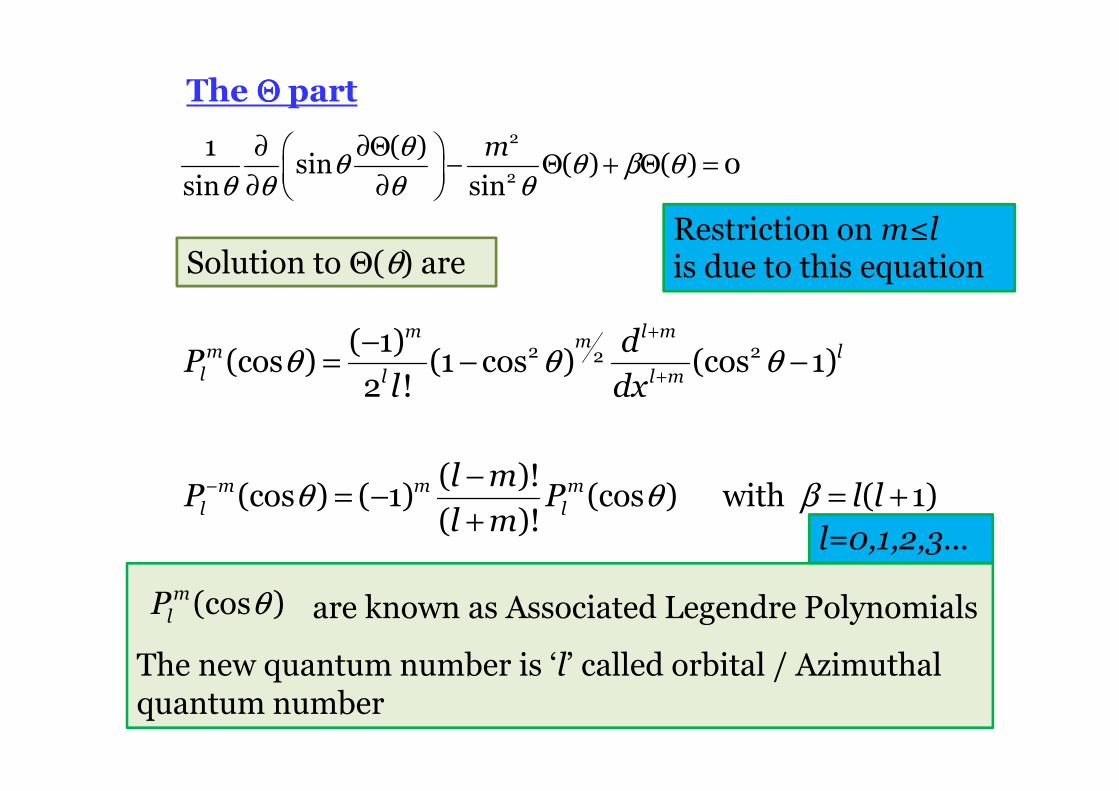
The ΘΘΘΘ part
are known as Associated Legendre Polynomials
The new quantum number is ‘l’ called orbital / Azimuthalquantum number
Restriction on m≤lis due to this equation
θθ θ β θ
θ θ θ θ
∂ ∂Θ − Θ + Θ =
∂ ∂
2
2
1 ( )sin ( ) ( ) 0
sin sin
m
θ θ θ
θ θ β
+
+
−
−= − −
−= − = +
+
2 22( 1)
(cos ) (1 cos ) (cos 1)2 !
( )!(cos ) ( 1) (cos ) with ( 1)
( )!
m l mmm ll l l m
m m ml l
dP
l dx
l mP P l l
l m
Solution to Θ(θ) are
θ(cos )mlP
l=0,1,2,3…
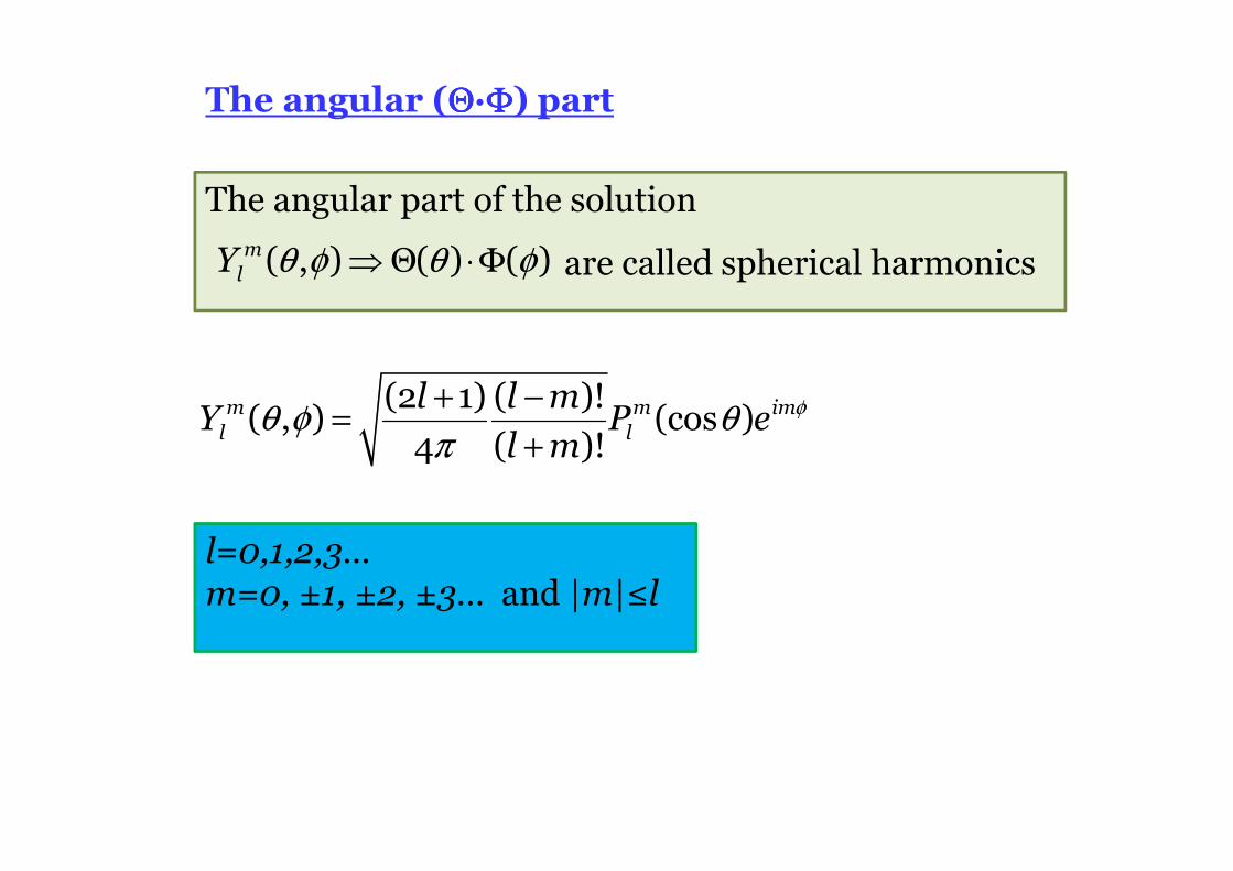
The angular (ΘΘΘΘ·ΦΦΦΦ) part
The angular part of the solution
are called spherical harmonicsθ φ θ φ⇒Θ ⋅Φ( , ) ( ) ( )mlY
φθ φ θπ
+ −=
+
(2 1) ( )!( , ) (cos )
4 ( )!m m iml l
l l mY P e
l m
l=0,1,2,3…m=0, ±1, ±2, ±3… and |m|≤l
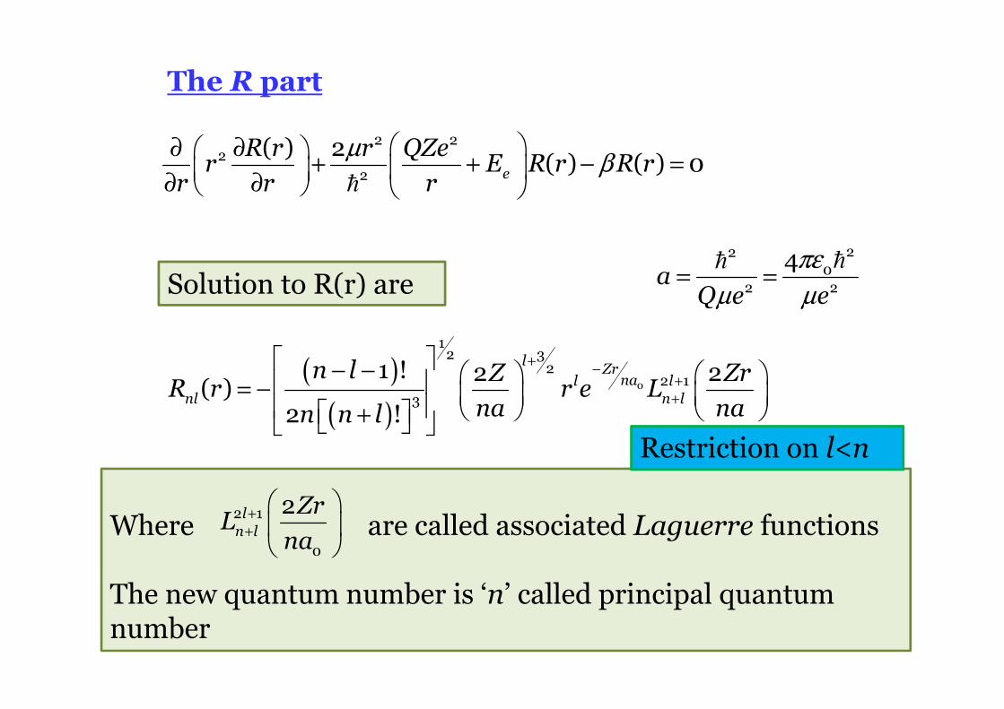
The R part
∂ ∂ + + − =
∂ ∂ �
2 22
2
( ) 2( ) ( ) 0e
R r r QZer E R r R r
r r rµ
β
( )
( )
+−
+
+
− − = − +
0
12 3
22 1
3
1 ! 2 2( )
2 !
lZrnal l
nl n l
n l Z ZrR r r e L
na nan n l
Solution to R(r) are
Where are called associated Laguerre functions
The new quantum number is ‘n’ called principal quantum number
+
+
2 1
0
2ln l
ZrL
na
= =��22
02 2
4aQ e e
πε
µ µ
Restriction on l<n
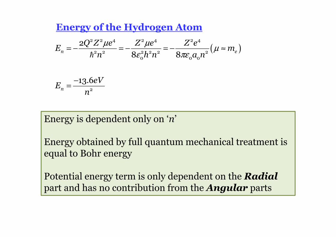
Energy of the Hydrogen Atom
( )= − = − = − ≈
−=
�
2 2 4 2 4 2 4
2 2 2 2 2 20 0 0
2
2
8 8
13.6
n e
n
Q Z e Z e Z eE m
n h n a n
eVE
n
µ µµ
ε πε
Energy is dependent only on ‘n’
Energy obtained by full quantum mechanical treatment is equal to Bohr energy
Potential energy term is only dependent on the Radialpart and has no contribution from the Angular parts
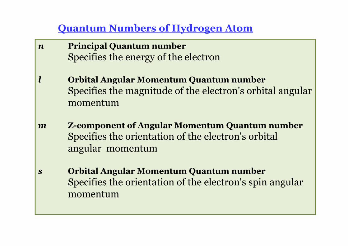
Quantum Numbers of Hydrogen Atom
n Principal Quantum number
Specifies the energy of the electron
l Orbital Angular Momentum Quantum number
Specifies the magnitude of the electron's orbital angular momentum
m Z-component of Angular Momentum Quantum number
Specifies the orientation of the electron's orbital angular momentum
s Orbital Angular Momentum Quantum number
Specifies the orientation of the electron's spin angular momentum
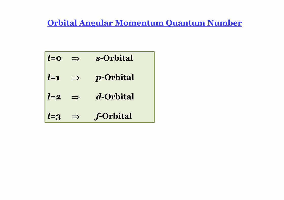
Orbital Angular Momentum Quantum Number
l=0 ⇒⇒⇒⇒ s-Orbital
l=1 ⇒⇒⇒⇒ p-Orbital
l=2 ⇒⇒⇒⇒ d-Orbital
l=3 ⇒⇒⇒⇒ f-Orbital
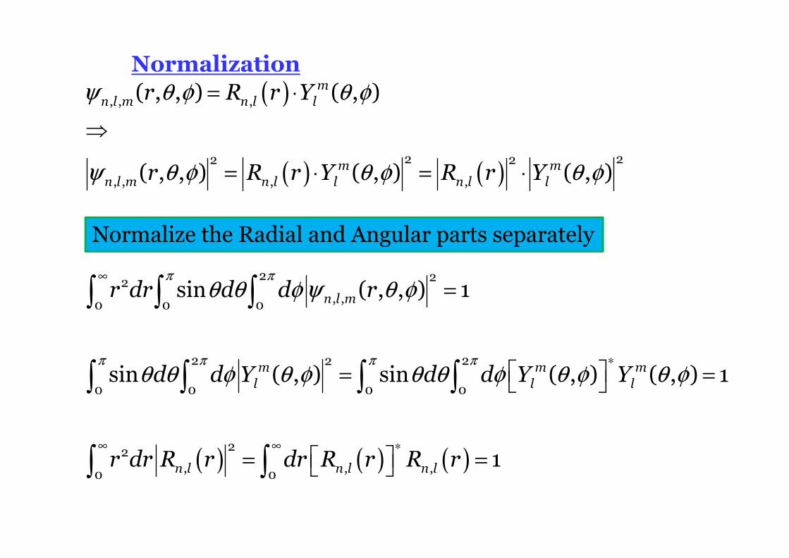
Normalization
( )
( ) ( )
( )
∞
∗
∞ ∞
= ⋅
⇒
= ⋅ = ⋅
=
= =
=
∫ ∫ ∫
∫ ∫ ∫ ∫
∫ ∫
, , ,
2 22 2
, , , ,
2 22, ,0 0 0
2 22
0 0 0 0
22, ,0 0
( , , ) ( , )
( , , ) ( , ) ( , )
sin ( , , ) 1
sin ( , ) sin ( , ) ( , ) 1
mn l m n l l
m mn l m n l l n l l
n l m
m m ml l l
n l n l
r R r Y
r R r Y R r Y
r dr d d r
d d Y d d Y Y
r dr R r dr R
π π
π π π π
ψ θ φ θ φ
ψ θ φ θ φ θ φ
θ θ φ ψ θ φ
θ θ φ θ φ θ θ φ θ φ θ φ
( ) ( )∗
= , 1n lr R r
Normalize the Radial and Angular parts separately
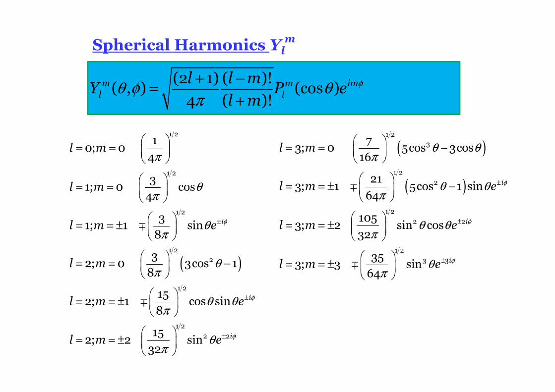
Spherical Harmonics Ylm
( )
φ
φ
φ
π
θπ
θπ
θπ
θ θπ
θπ
±
±
±
= =
= =
= = ±
= = −
= = ±
= = ±
∓
∓
1 2
1 2
1 2
1 22
1 2
1 2
2 2
10; 0
4
31; 0 cos
4
31; 1 sin
8
32; 0 3cos 1
8
152; 1 cos sin
8
152; 2 sin
32
i
i
i
l m
l m
l m e
l m
l m e
l m e
( )
( ) φ
φ
φ
θ θπ
θ θπ
θ θπ
θπ
±
±
±
= = −
= = ± −
= = ±
= = ±
∓
∓
1 23
1 2
2
1 2
2 2
1 2
3 3
73; 0 5cos 3cos
16
213; 1 5cos 1 sin
64
1053; 2 sin cos
32
353; 3 sin
64
i
i
i
l m
l m e
l m e
l m e
φθ φ θπ
+ −=
+
(2 1) ( )!( , ) (cos )
4 ( )!m m iml l
l l mY P e
l m
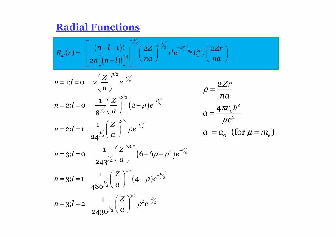
Radial Functions
( )
( )
( )
ρ
ρ
ρ
ρ
ρ
ρ
ρ
ρ
ρ ρ
ρ
ρ
−
−
−
−
−
−
= =
= = −
= =
= = − −
= = −
= =
3 2
2
3 2
212
3 2
212
3 22 2
12
3 2
212
3 22 2
12
1; 0 2
12; 0 2
8
12; 1
24
13; 0 6 6
243
13; 1 4
486
13; 2
2430
Zn l e
a
Zn l e
a
Zn l e
a
Zn l e
a
Zn l e
a
Zn l e
a
ρ
πε
µ
µ
=
=
= =
�2
02
0
2
4
(for )e
Zr
na
ae
a a m
( )
( )
+−
+
+
− − = − +
0
12 3
22 1
3
1 ! 2 2( )
2 !
l Zrnal l
nl n l
n l Z ZrR r r e L
na nan n l
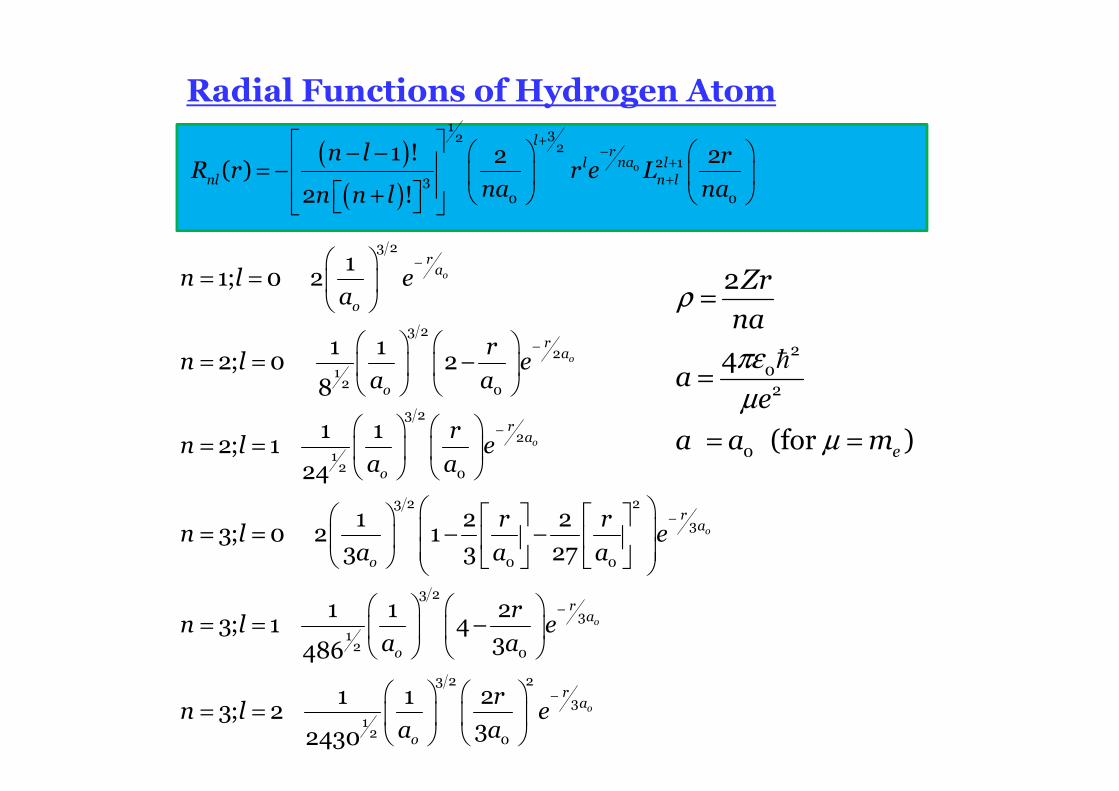
Radial Functions of Hydrogen Atom
−
−
−
−
= =
= = −
= =
= = − −
= =
3 2
3 2
212 0
3 2
212 0
3 2 2
3
0 0
12
11; 0 2
1 12; 0 2
8
1 12; 1
24
1 2 23; 0 2 1
3 3 27
1 13; 1
486
o
o
o
o
ra
o
ra
o
ra
o
ra
o
o
n l ea
rn l e
a a
rn l e
a a
r rn l e
a a a
n la
−
−
−
= =
3 2
3
0
3 2 2
312 0
24
3
1 1 23; 2
32430
o
o
ra
ra
o
re
a
rn l e
a a
( )
( )
+−
+
+
− − = − +
0
1 322
2 13
0 0
1 ! 2 2( )
2 !
lrnal l
nl n l
n l rR r r e L
na nan n l
ρ
πε
µ
µ
=
=
= =
�2
02
0
2
4
(for )e
Zr
na
ae
a a m
Wavefunctions of Hydrogen Atom
φ
ψ ψπ
ψ ψπ
ψ ψ θπ
ψ ψ θπ
ψ ψπ
+
−
−
−
−
−
+
−
= =
= = −
= =
= =
= =
1
1
3 2
1,0,0 1
3 2
22,0,0 2
0
3 2
22,1,0 2
0
3 2
22,1, 1 2
0
3 2
2,1, 1 20
1 1
1 12
4 2
1 1cos
4 2
1 1sin
8
1 1
8
o
o
o
z
o
ra
so
ra
so
ra
po
ra i
po
po
ea
re
a a
re
a a
re e
a a
r
a aφθ
−−
2 sin o
ra ie e
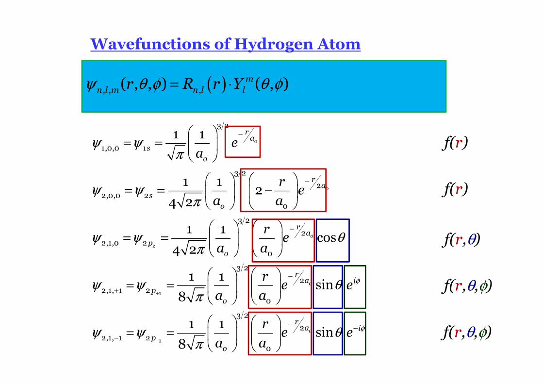
( )ψ θ φ θ φ= ⋅, , ,( , , ) ( , )mn l m n l lr R r Y
f(r)
f(r)
f(r,θ)
f(r,θ,φ)
f(r,θ,φ)
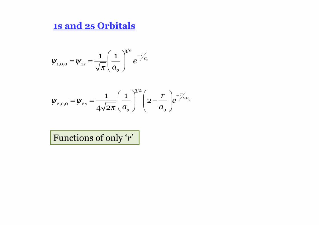
1s and 2s Orbitals
ψ ψπ
ψ ψπ
−
−
= =
= = −
3 2
1,0,0 1
3 2
22,0,0 2
0
1 1
1 12
4 2
o
o
ra
so
ra
so
ea
re
a a
Functions of only ‘r’
φ
φ
ψ ψ θπ
ψ ψ θπ
ψ ψ θπ
+
−
−
−
+
−−
−
= =
= =
= =
1
1
3 2
22,1,0 2
0
3 2
22,1, 1 2
0
3 2
22,1, 1 2
0
1 1cos
4 2
1 1sin
8
1 1sin
8
o
z
o
o
ra
po
ra i
po
ra i
po
re
a a
re e
a a
re e
a a
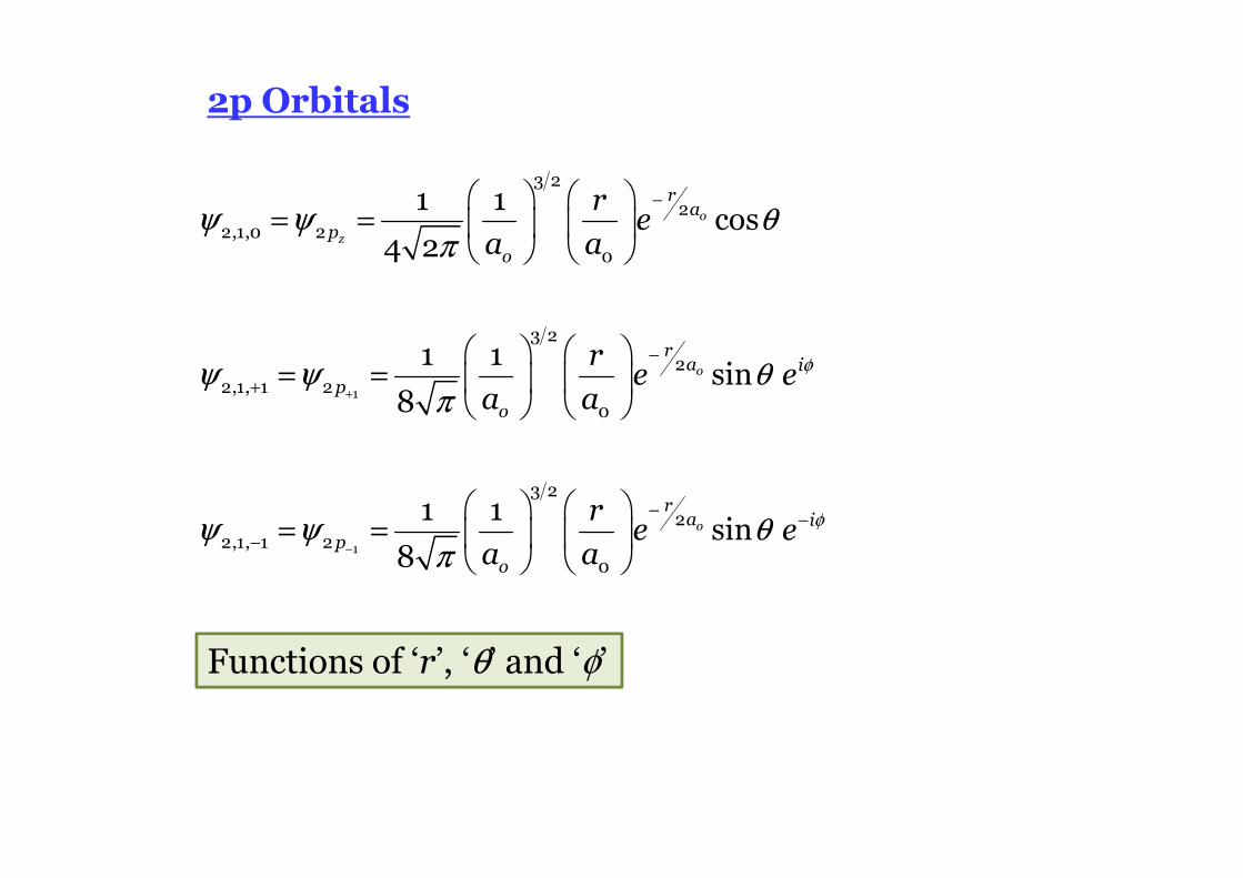
2p Orbitals
Functions of ‘r’, ‘θ’ and ‘φ’
φ
φ
ψ ψ θπ
ψ ψ θπ
ψ ψ θπ
+
−
−
−
+
−−
−
= =
= =
= =
1
1
3 2
22,1,0 2
0
3 2
22,1, 1 2
0
3 2
22,1, 1 2
0
1 1cos
4 2
1 1sin
8
1 1sin
8
o
z
o
o
ra
po
ra i
po
ra i
po
re
a a
re e
a a
re e
a a
2p Orbitals
( )
( )
ψ θ φ ψ ψπ
ψ θ φ ψ ψπ
−
+ −
−
+ −
= +
= −
3 2
22 2,1, 1 2,1, 1
0
3 2
22 2,1, 1 2,1, 1
0
1 1 1sin cos =
32 2
1 1 1sin sin =
32 2
o
x
o
y
ra
po
ra
po
re
a a
re
a a i
Linear combination
Radial functions
ρψ −′=1001s N e ( )
ρ
ψ ρ−
′′= −200 22 2s N e
ρ =0
r
a
ρ
ψ ρ θ−
′′′=210 22 coszpN e
For s-Orbitals the maximum probability denisty of finding the electron is on the nucleus
For s-Orbitals the probability of finding the electron on the nucleus zero
Surface plots
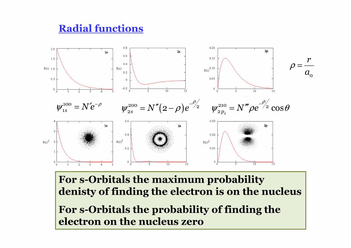
Surface plot of the ΨΨΨΨ2s ; 2s wavefunction (orbital) of the hydrogen atom. The
height of any point on the surface above the xy plane (the nuclear plane)
represents the magnitude of the ΨΨΨΨ2s function at the at point (x,y) in the
nuclear plane. Note that there is a negative region (depression) about the
nucleus; the negative region begins at r=2a0 an goes asymptotically to zero at
r=∞∞∞∞.
Surface plot of the |ΨΨΨΨ2s|2; the probability density associated with
the 1s wavefunction of the hydrogen atom. Note that the negative
region of the 2s plot on the left now appears as positive region.
Surface plot of the 1s wavefunction (orbital) of the hydrogen atom. The height
of any point on the surface above the xy plane (the nuclear plane) represents
the magnitude of the ΨΨΨΨ1s function at the at point (x,y) in the nuclear plane.
The nucleus is located in the xy place immediately below the ‘peak’
Surface plot of the |ΨΨΨΨ1s|2; the probability density associated with
the 1s wavefunction of the hydrogen atom.
1s
2s
(1s)2
(2s)2
Surface plots
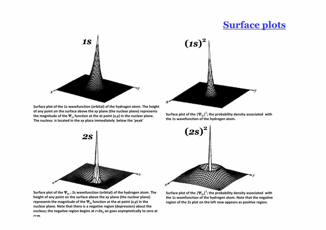
R(2pz)
(2pz)2
Surface plot of radial portion of a 2p wavefunction of the hydrogen
atom. The gird lines have been left transparent so that the inner
‘hollow’ portion is visible.
Profile of the radial portion of a 2p wavefunction of the hydrogen atom.
Profile of the 2pz orbital along the z-azis. Surface plot of the 2pz wavefunction (orbital)
in the xz (or yz) plane for the hydrogen atom.
The ‘pit’ represents the negative lobe and the
‘hill’ the positive lobe of a 2p orbital.
Surface plot of the (2pz)2; the probability density
associated with the 2pz wavefunction of the
hydrogen atom. Each of the hills represents and
area in the xz (or yz) plane where the probability
density is the highest, The probability density
along the x (or y) axis passing through the nucleus
(0,0) is everywhere zero.
2pz2pz
R(2pz)
Surface plots
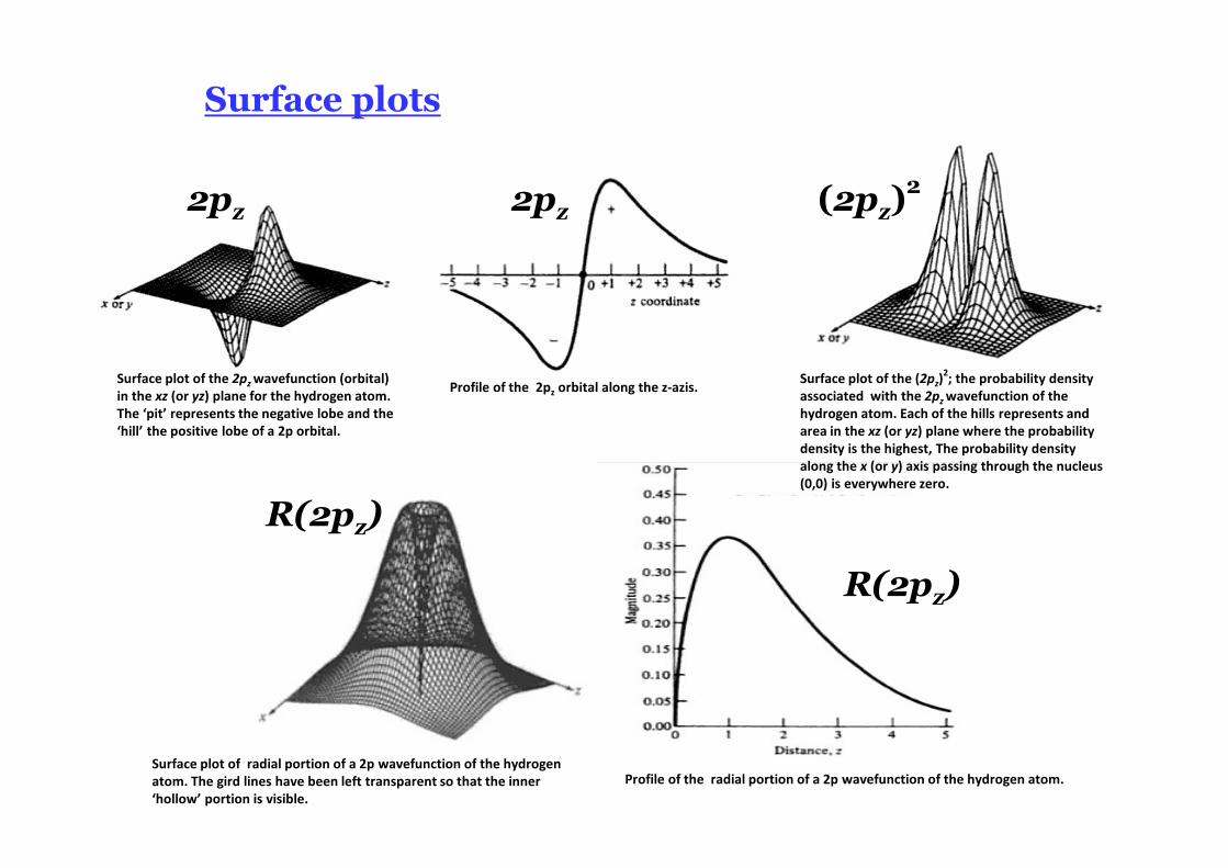
Surface plot of the 3dz2 wavefunction (orbital) in the xz (or yz) plane for the
hydrogen atom. The large hills correspond to the positive lobes and the
small pits correspond to the negative lobes.
Surface plot of the (3dz2 )2 the probability density associated with the 3dz2
orbital of the hydrogen atom. This figure is rotated with respect to the
figure on the left so that the small hill will be clearly visible. Another
smaller hill is hidden behind the large hill.
Surface plot of the 3dxy wavefunction (orbital) in the xz plane for the
hydrogen atom. The hills and the pits have same amplitude. Surface plot of the (3dxy )2 the probability density associated with the 3dxy
orbital of the hydrogen atom. Pits in the figure to the left appear has hills.
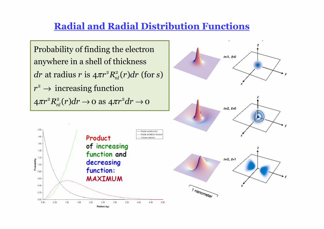
Radial and Radial Distribution Functions
π
π π
→
→ →
2 2
2
2 2 2
Probability of finding the electron
anywhere in a shell of thickness
at radius is 4 ( ) (for )
increasing function
4 ( ) 0 as 4 0
nl
nl
dr r r R r dr s
r
r R r dr r dr
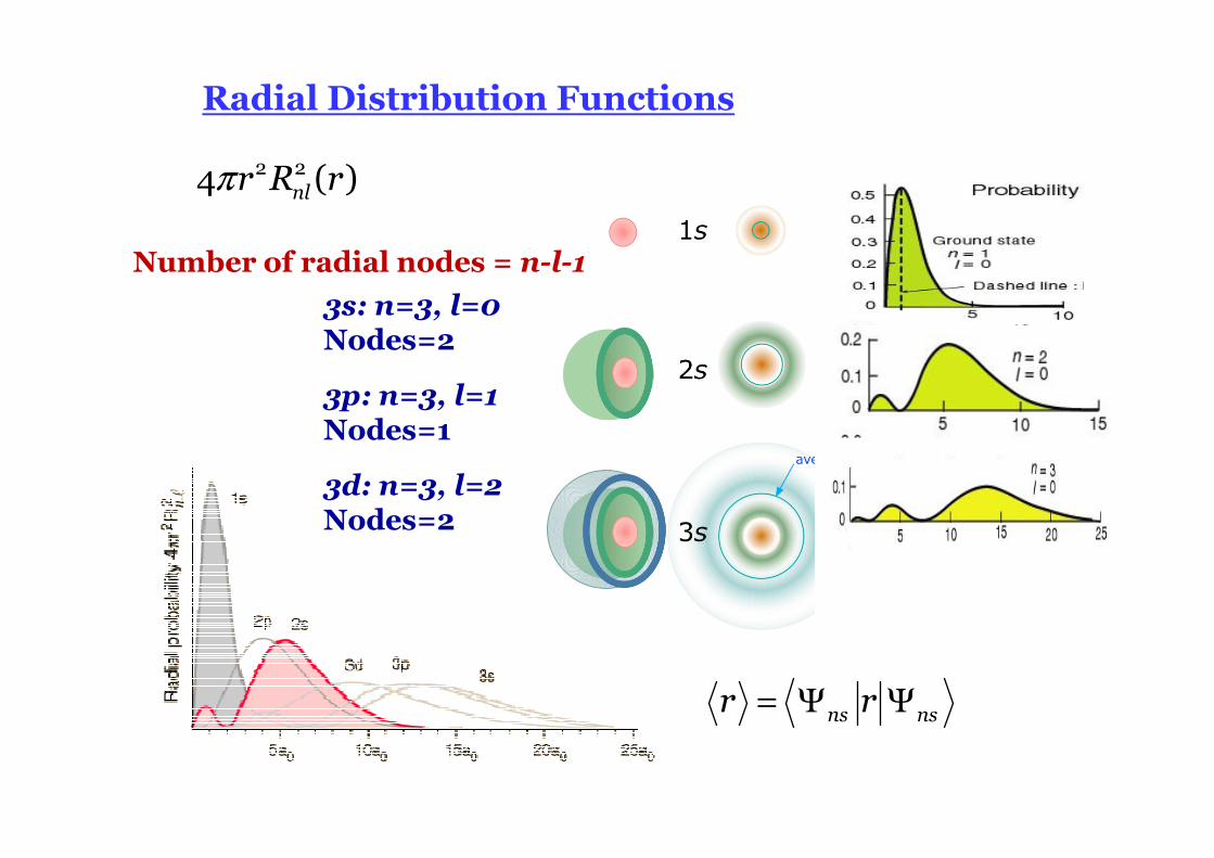
Radial Distribution Functions
π 2 24 ( )nlr R r
3s: n=3, l=0Nodes=2
3p: n=3, l=1Nodes=1
3d: n=3, l=2Nodes=2
= Ψ Ψns nsr r
Number of radial nodes = n-l-1
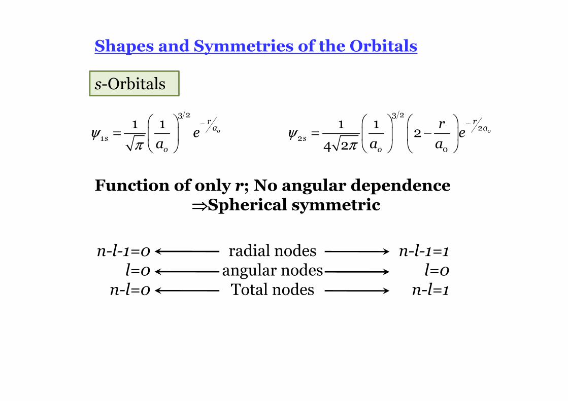
Shapes and Symmetries of the Orbitals
s-Orbitals
ψ ψπ π
− − = = −
3 2 3 2
21 2
0
1 1 1 1 2
4 2o o
r ra a
s so o
re e
a a a
Function of only r; No angular dependence⇒⇒⇒⇒Spherical symmetric
n-l-1=0l=0
n-l=0
radial nodesangular nodesTotal nodes
n-l-1=1l=0n-l=1
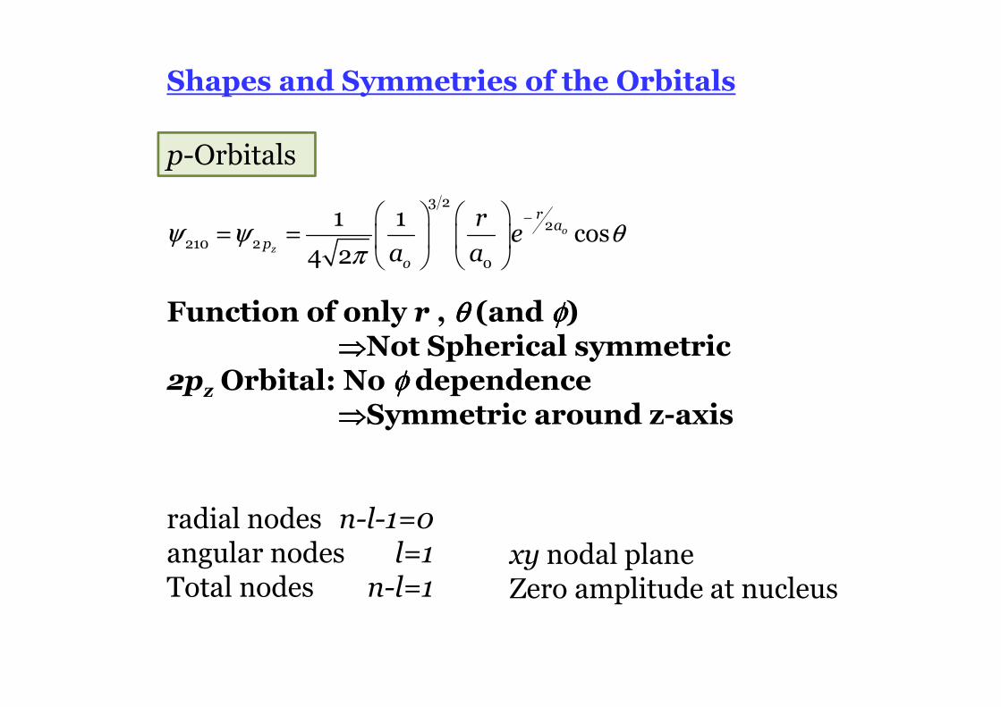
Shapes and Symmetries of the Orbitals
p-Orbitals
Function of only r , θθθθ (and φφφφ)⇒⇒⇒⇒Not Spherical symmetric
2pz Orbital: No φφφφ dependence⇒⇒⇒⇒Symmetric around z-axis
radial nodesangular nodesTotal nodes
n-l-1=0l=1
n-l=1
ψ ψ θπ
− = =
3 2
2210 2
0
1 1cos
4 2o
z
ra
po
re
a a
xy nodal planeZero amplitude at nucleus
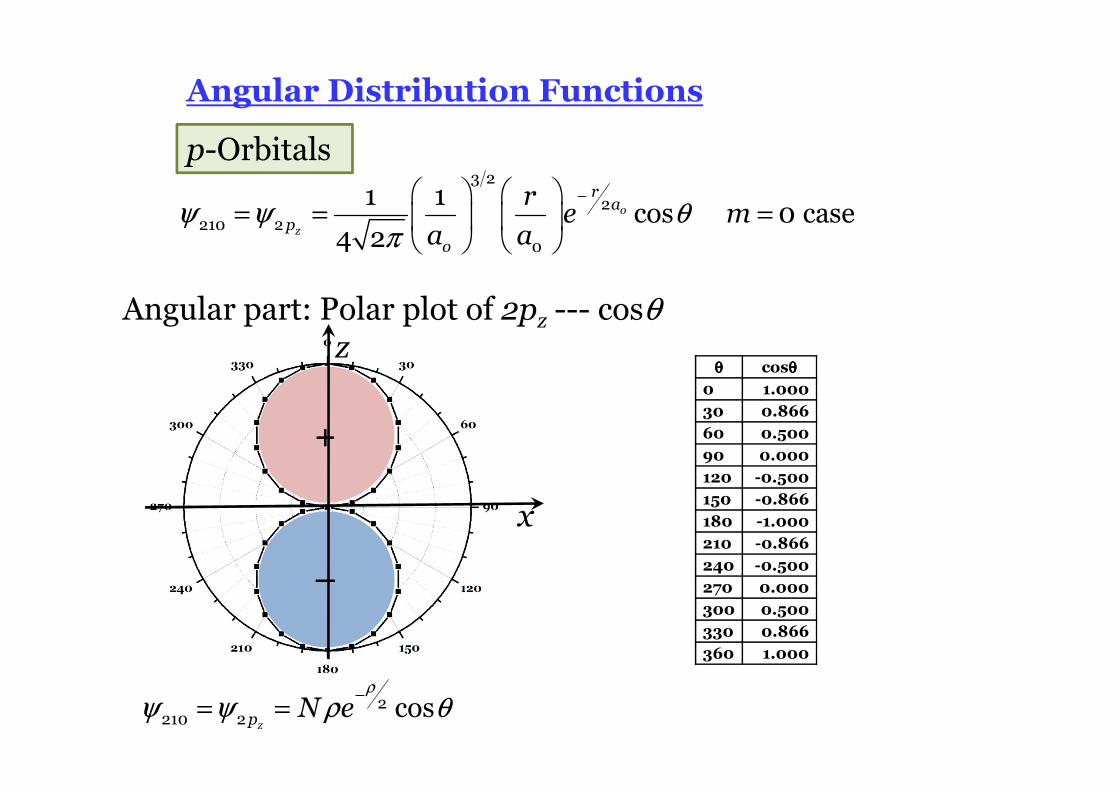
Angular Distribution Functions
p-Orbitals
ψ ψ θπ
− = = =
3 2
2210 2
0
1 1cos 0 case
4 2o
z
ra
po
re m
a a
+
–
θθθθ cosθθθθ
0 1.000
30 0.866
60 0.500
90 0.000
120 -0.500
150 -0.866
180 -1.000
210 -0.866
240 -0.500
270 0.000
300 0.500
330 0.866
360 1.000
ρ
ψ ψ ρ θ−
= = 2210 2 cos
zpN e
Angular part: Polar plot of 2pz --- cosθ
x
z
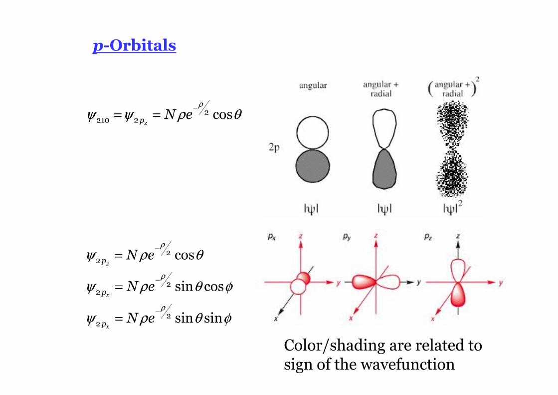
p-Orbitals
ρ
ψ ψ ρ θ−
= = 2210 2 cos
zpN e
ρ
ρ
ρ
ψ ρ θ
ψ ρ θ φ
ψ ρ θ φ
−
−
−
=
=
=
22
22
22
cos
sin cos
sin sin
z
x
x
p
p
p
N e
N e
N e
Color/shading are related to sign of the wavefunction
d-Orbitals
ρ
ρ
ρ
ρ
ρ
ψ ρ θ
ψ ρ θ θ φ
ψ ρ θ θ φ
ψ ρ θ φ
ψ ρ θ φ
−
−
−
−
−
−
= −
=
=
=
=
2
2 2
2 2 313
2 33 2
2 33 3
2 2 33 4
2 2 33 5
(3cos 1)
(sin cos cos )
(sin cos sin )
(sin cos2 )
(sin sin2 )
z
xz
yz
x y
xy
d
d
d
d
d
N e
N e
N e
N e
N e
Angular part
Blue: -veYellow: +ve
Angular + Radial
n=3; l=2; m=0,±1, ±2
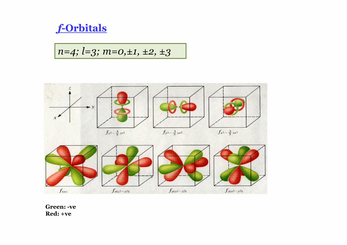
f-Orbitals
n=4; l=3; m=0,±1, ±2, ±3
Green: -veRed: +ve
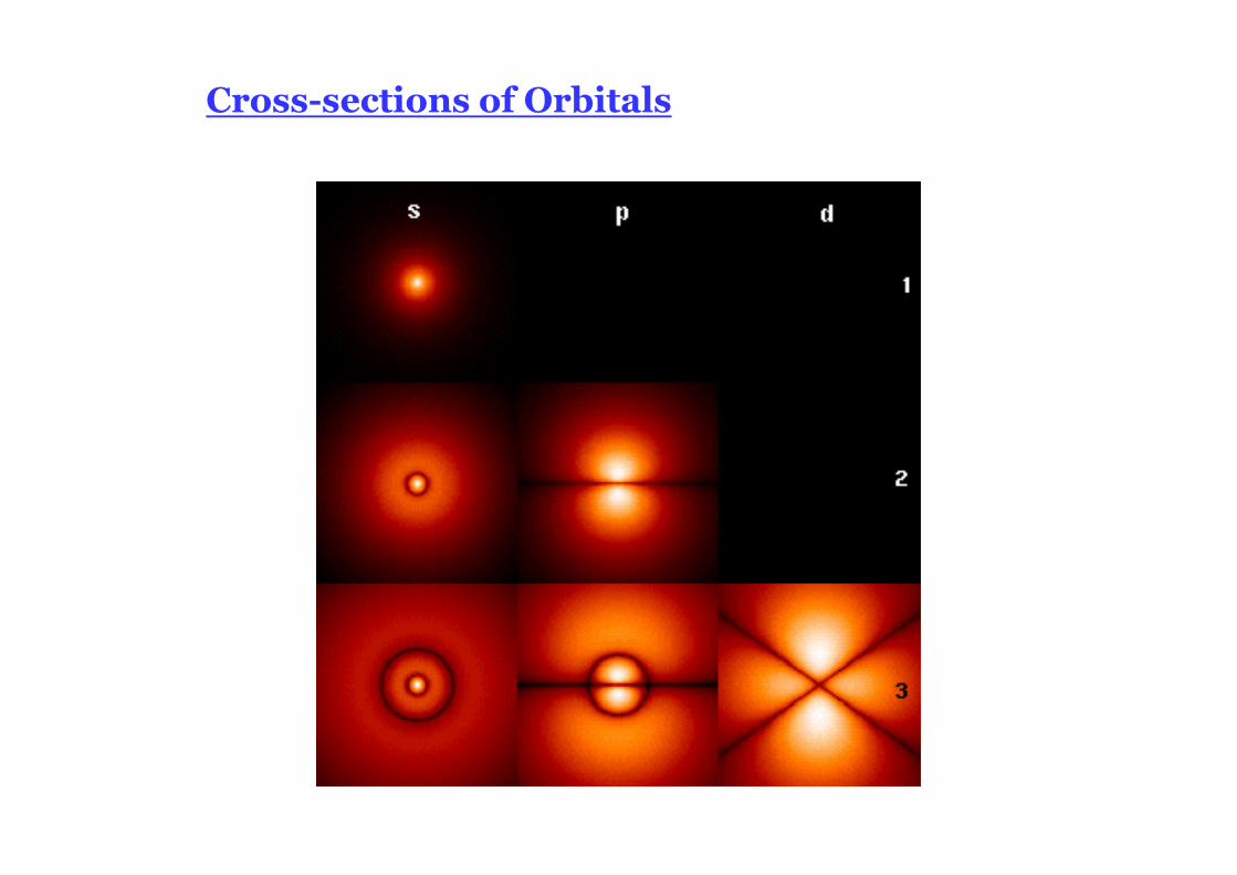
Cross-sections of Orbitals
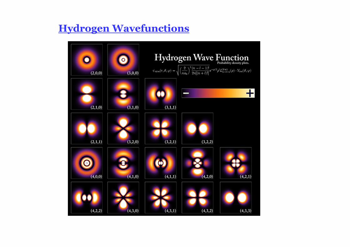
Hydrogen Wavefunctions
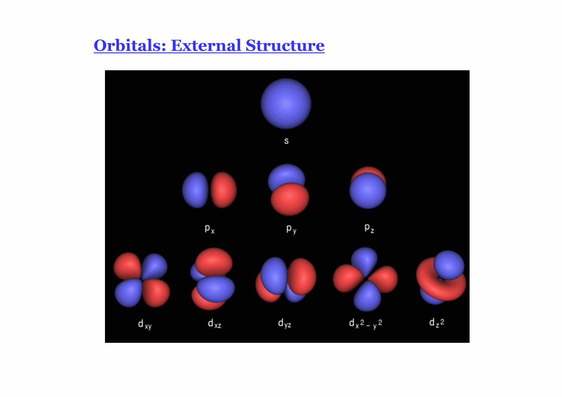
Orbitals: External Structure
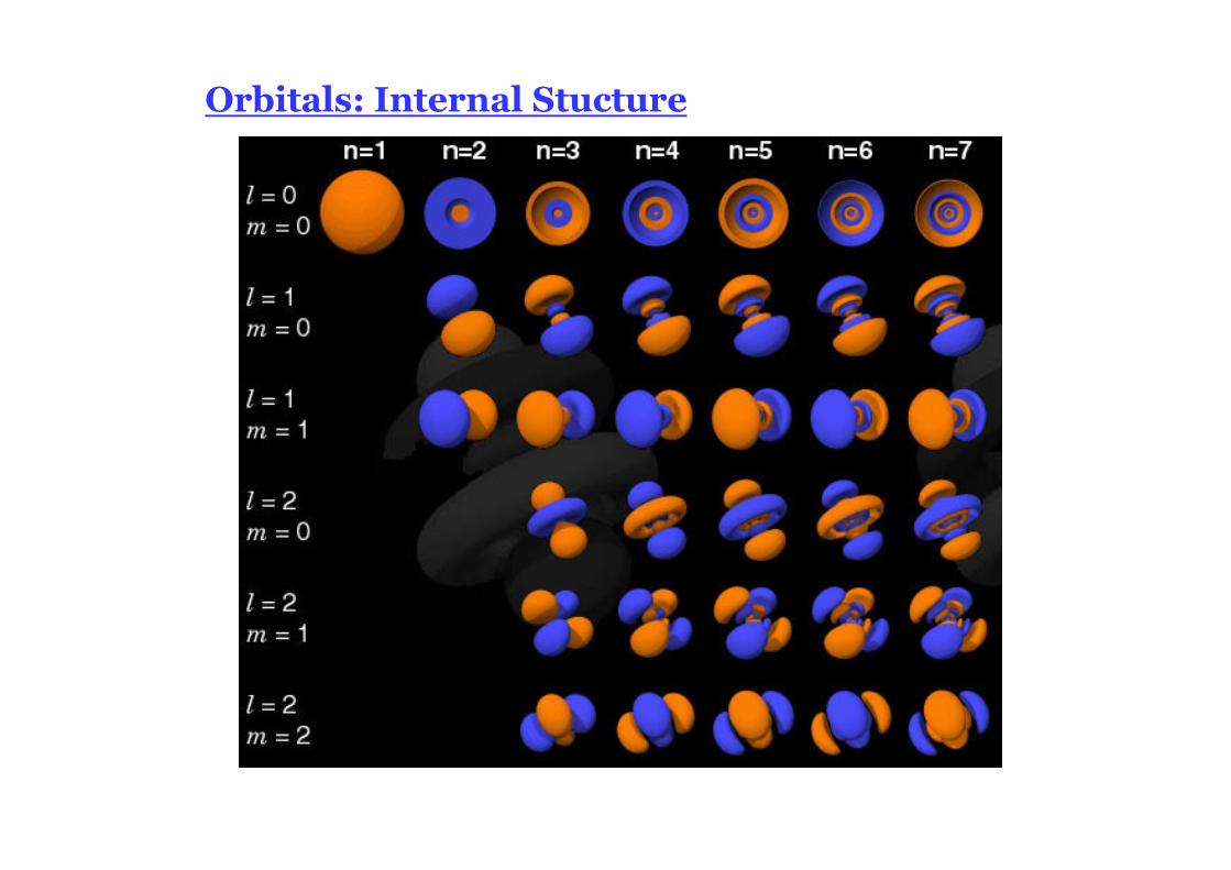
Orbitals: Internal Stucture
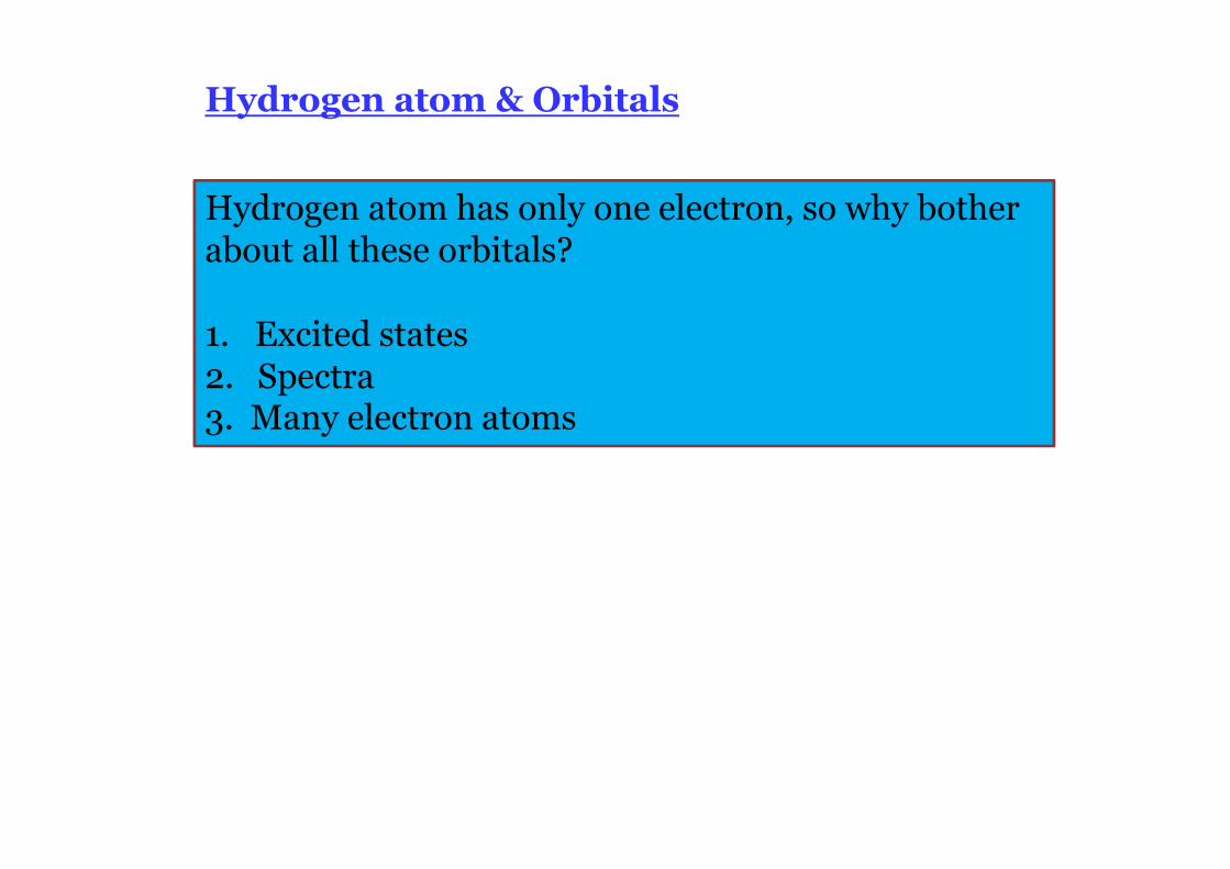
Hydrogen atom & Orbitals
Hydrogen atom has only one electron, so why bother about all these orbitals?
1. Excited states2. Spectra3. Many electron atoms
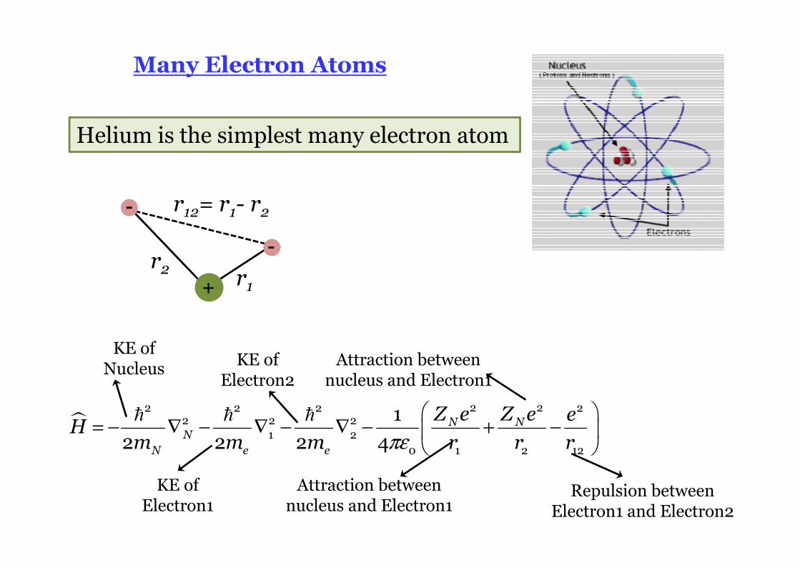
Many Electron Atoms
Helium is the simplest many electron atom
+
-
-
r1r2
r12= r1- r2
�
πε
= − ∇ − ∇ − ∇ − + −
� � �2 22 2 2 2
2 2 21 2
0 1 2 12
12 2 2 4
N NN
N e e
Z e Z e eH
m m m r r r
KE of Nucleus
KE of Electron1
KE of Electron2
Attraction between nucleus and Electron1
Attraction between nucleus and Electron1
Repulsion between Electron1 and Electron2
Helium Atom
�
�
� �
� �
= − ∇ − ∇ − ∇ − + −
= − ∇ − ∇ − − ∇ − + =
= − ∇ = − ∇ − − ∇ − +
=
� � �
� � �
� � �
2 22 2 2 22 2 2
1 20 1 2 12
2 22 2 2 22 2 2
1 21 2 12 0
2 22 2 2 22 2 2
1 21 2 12
1
2 2 2 4
1;
2 2 2 4
2 2 2
N NN
N e e
N NN
N e e
N NN eN
N e e
N eN n N
Z e Z e eH
m m m r r r
QZ e QZ e QeH Q
m m r m r r
QZ e QZ e QeH H
m m r m r r
H E H
πε
πε
χ χ ψ =e e eE ψ
Helium Atom
�
� � �
� �
= − ∇ − − ∇ − +
= + +
= − ∇ − = − ∇ −
� �
� �
2 22 2 22 21 2
1 2 12
2
1 2
12
2 22 22 2
1 21 21 2
2 2
and 2 2
N Ne
e e
e
N N
e e
QZ e QZ e QeH
m r m r r
QeH H H
r
QZ e QZ eH H
m r m r
The Hamiltonians Ĥ1 and Ĥ1 are one electron Hamiltonians similar to that of hydrogen atom
� � �= +
+
1 21 1 1 2 2 2 1 1 1 2 2 2 1 1 1 2 2 2
2
1 1 1 2 2 212
( , , , , , ) ( , , , , , ) ( , , , , , )
( , , , , , )
e e e e
e
H r r H r r H r r
Qer r
r
ψ θ φ θ φ ψ θ φ θ φ ψ θ φ θ φ
ψ θ φ θ φ
Orbital Approximation
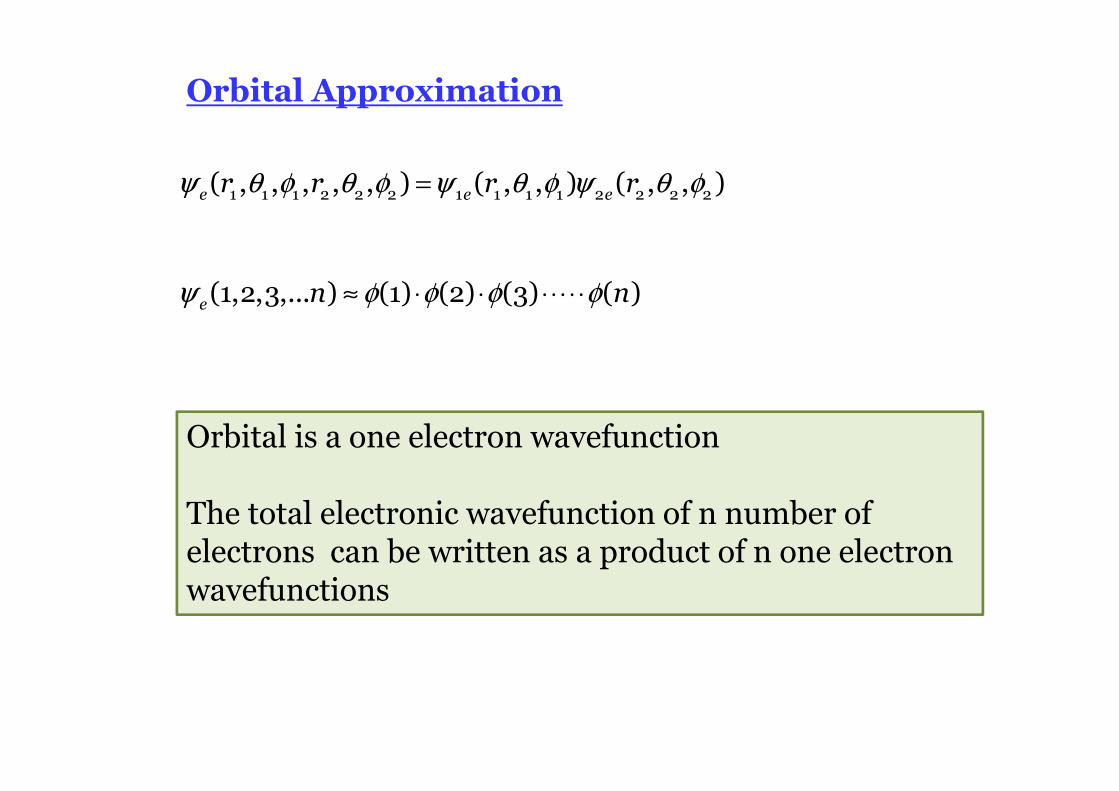
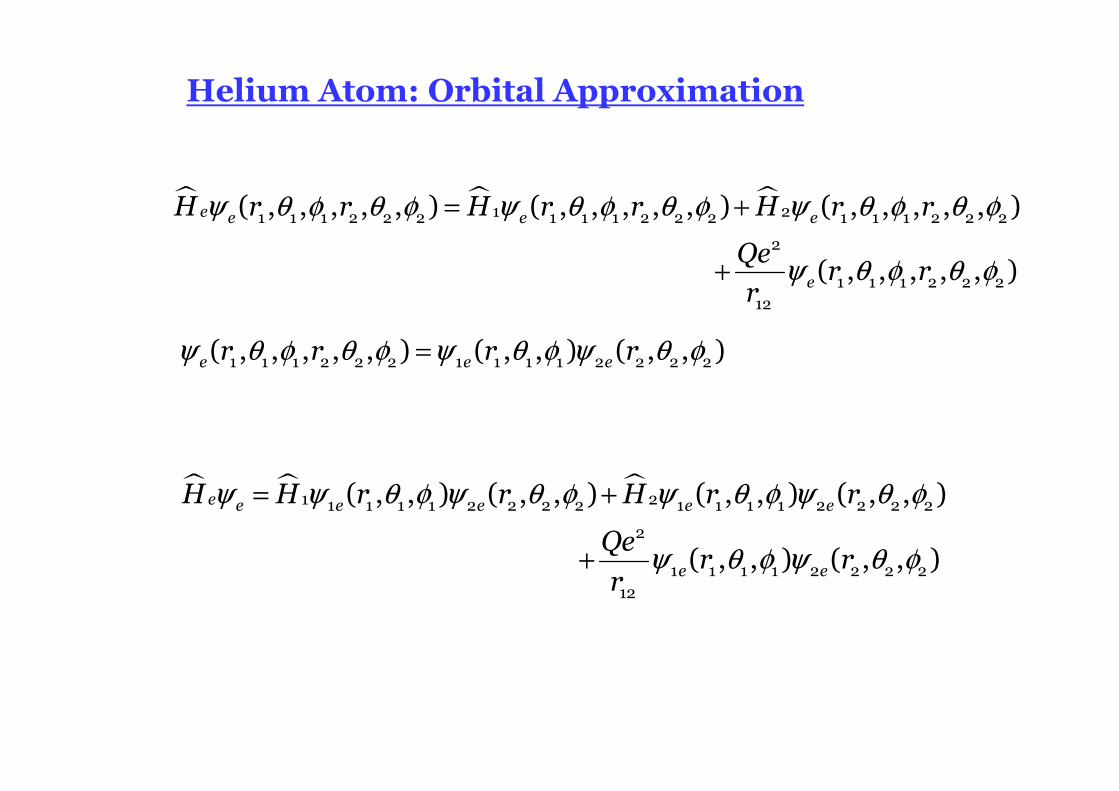
ψ θ φ θ φ ψ θ φ ψ θ φ=1 1 1 2 2 2 1 1 1 1 2 2 2 2( , , , , , ) ( , , ) ( , , )e e er r r r
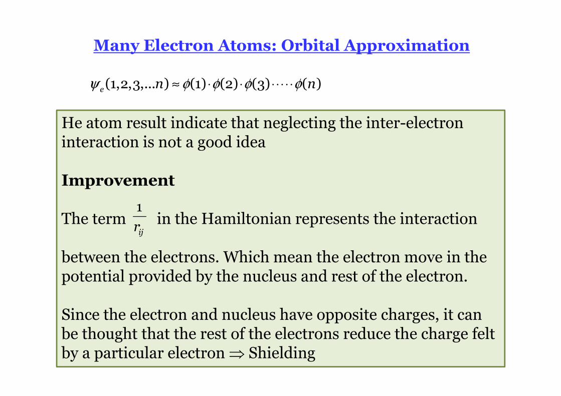
ψ φ φ φ φ≈ ⋅ ⋅ ⋅⋅⋅ ⋅ ⋅(1,2,3,... ) (1) (2) (3) ( )e n n
Orbital is a one electron wavefunction
The total electronic wavefunction of n number of electrons can be written as a product of n one electron wavefunctions
� � �= +
+
1 21 1 1 2 2 2 1 1 1 2 2 2 1 1 1 2 2 2
2
1 1 1 2 2 212
( , , , , , ) ( , , , , , ) ( , , , , , )
( , , , , , )
e e e e
e
H r r H r r H r r
Qer r
r
ψ θ φ θ φ ψ θ φ θ φ ψ θ φ θ φ
ψ θ φ θ φ
ψ θ φ θ φ ψ θ φ ψ θ φ=1 1 1 2 2 2 1 1 1 1 2 2 2 2( , , , , , ) ( , , ) ( , , )e e er r r r
� � �= +
+
1 21 1 1 1 2 2 2 2 1 1 1 1 2 2 2 2
2
1 1 1 1 2 2 2 212
( , , ) ( , , ) ( , , ) ( , , )
( , , ) ( , , )
e e e e e e
e e
H H r r H r r
Qer r
r
ψ ψ θ φ ψ θ φ ψ θ φ ψ θ φ
ψ θ φ ψ θ φ
Helium Atom: Orbital Approximation
� � �ψ ψ θ φ ψ θ φ ψ θ φ ψ θ φ
ψ θ φ ψ θ φ
= +
+
1 21 1 1 1 2 2 2 2 1 1 1 1 2 2 2 2
2
1 1 1 1 2 2 2 212
( , , ) ( , , ) ( , , ) ( , , )
( , , ) ( , , )
e e e e e e
e e
H H r r H r r
Qer r
r
Helium Atom: Orbital Approximation
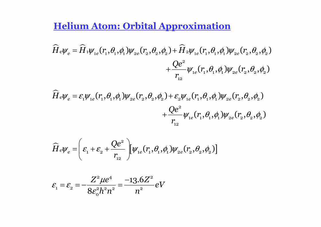
� ψ ε ψ θ φ ψ θ φ ε ψ θ φ ψ θ φ
ψ θ φ ψ θ φ
= +
+
1 1 1 1 1 2 2 2 2 2 1 1 1 1 2 2 2 2
2
1 1 1 1 2 2 2 212
( , , ) ( , , ) ( , , ) ( , , )
( , , ) ( , , )
e e e e e e
e e
H r r r r
Qer r
r
� [ ]ψ ε ε ψ θ φ ψ θ φ
= + +
2
1 2 1 1 1 1 2 2 2 212
( , , ) ( , , )e e e e
QeH r r
r
µε ε
ε
−= = − =
2 4 2
1 2 2 2 2 20
13.68Z e Z
eVh n n
Helium Atom: Orbital Approximation
� [ ]ψ ε ε ψ θ φ ψ θ φ
= + +
2
1 2 1 1 1 1 2 2 2 212
( , , ) ( , , )e e e e
QeH r r
r
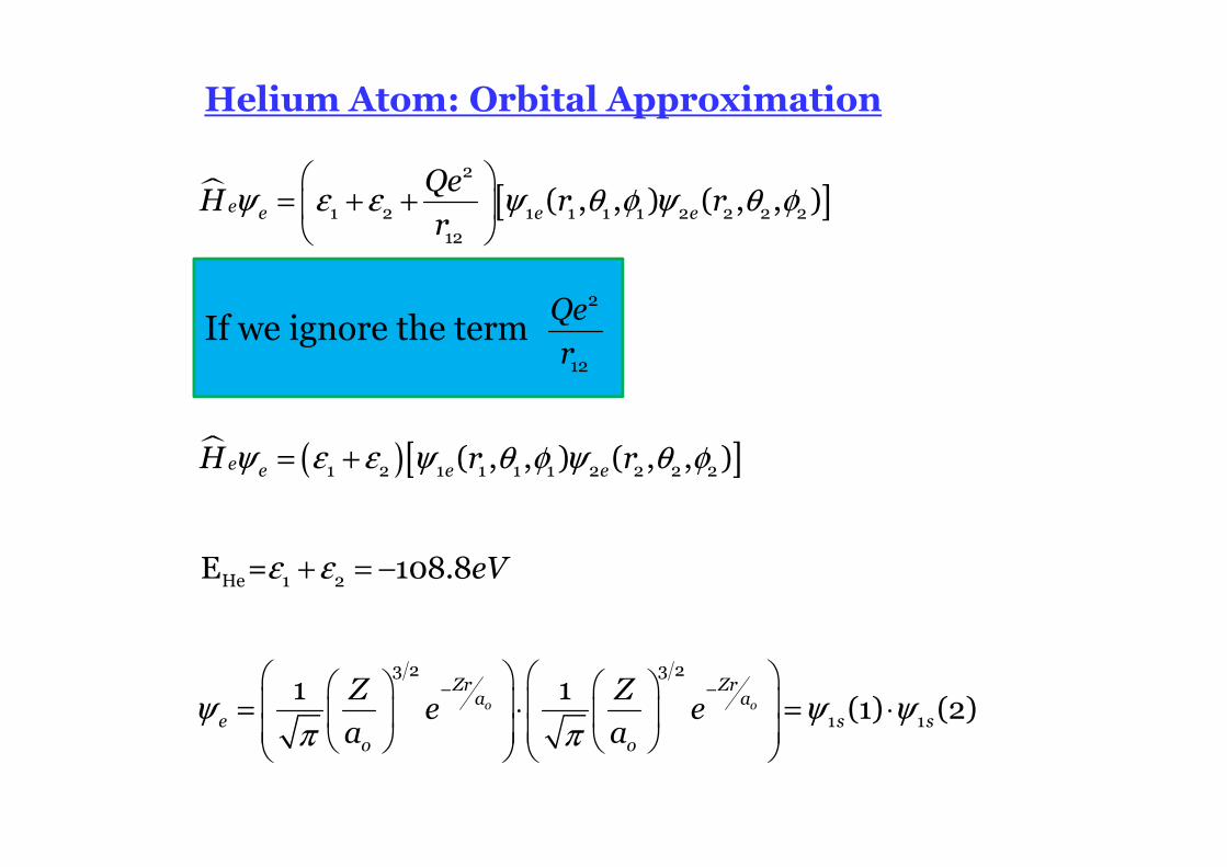
If we ignore the term 2
12
Qe
r
� ( )[ ]ψ ε ε ψ θ φ ψ θ φ= +1 2 1 1 1 1 2 2 2 2( , , ) ( , , )e e e eH r r
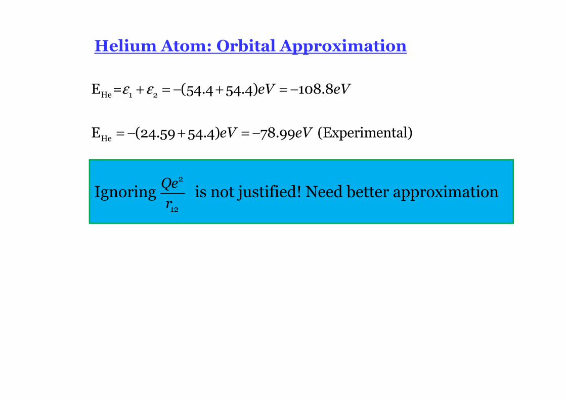
ε ε+ = −He 1 2E = 108.8eV
ψ ψ ψπ π
− − = ⋅ = ⋅
3 2 3 2
1 1
1 1(1) (2)o o
Zr Zra a
e s so o
Z Ze e
a a
Helium Atom: Orbital Approximation
ε ε+ = − + = −
= − + = −
He 1 2
He
E = (54.4 54.4) 108.8
E (24.59 54.4) 78.99 (Experimental)
eV eV
eV eV
Ignoring is not justified! Need better approximation2
12
Qe
r
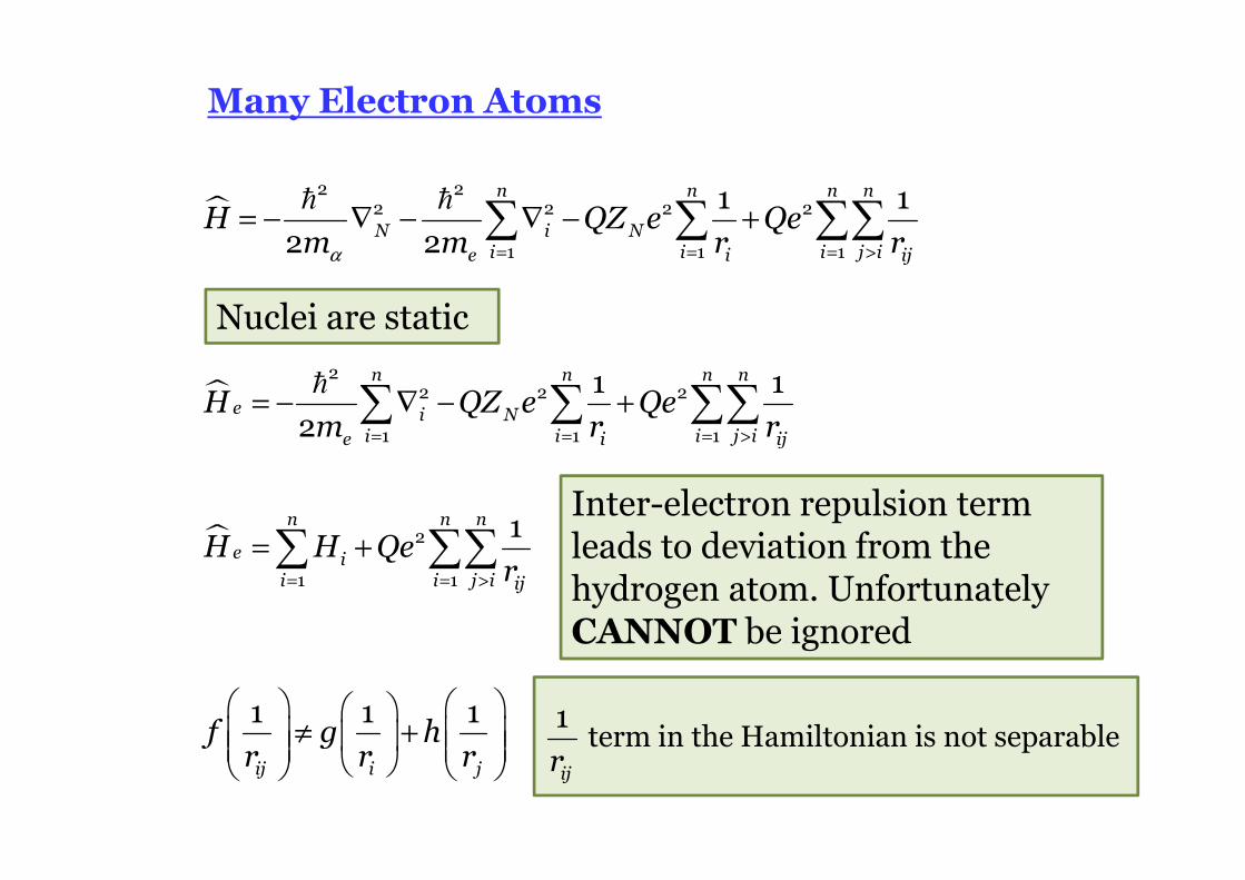
Many Electron Atoms
�
α = = = >
= − ∇ − ∇ − +∑ ∑ ∑∑� �2 2
2 2 2 2
1 1 1
1 1
2 2
n n n n
N i Ni i i j ie i ij
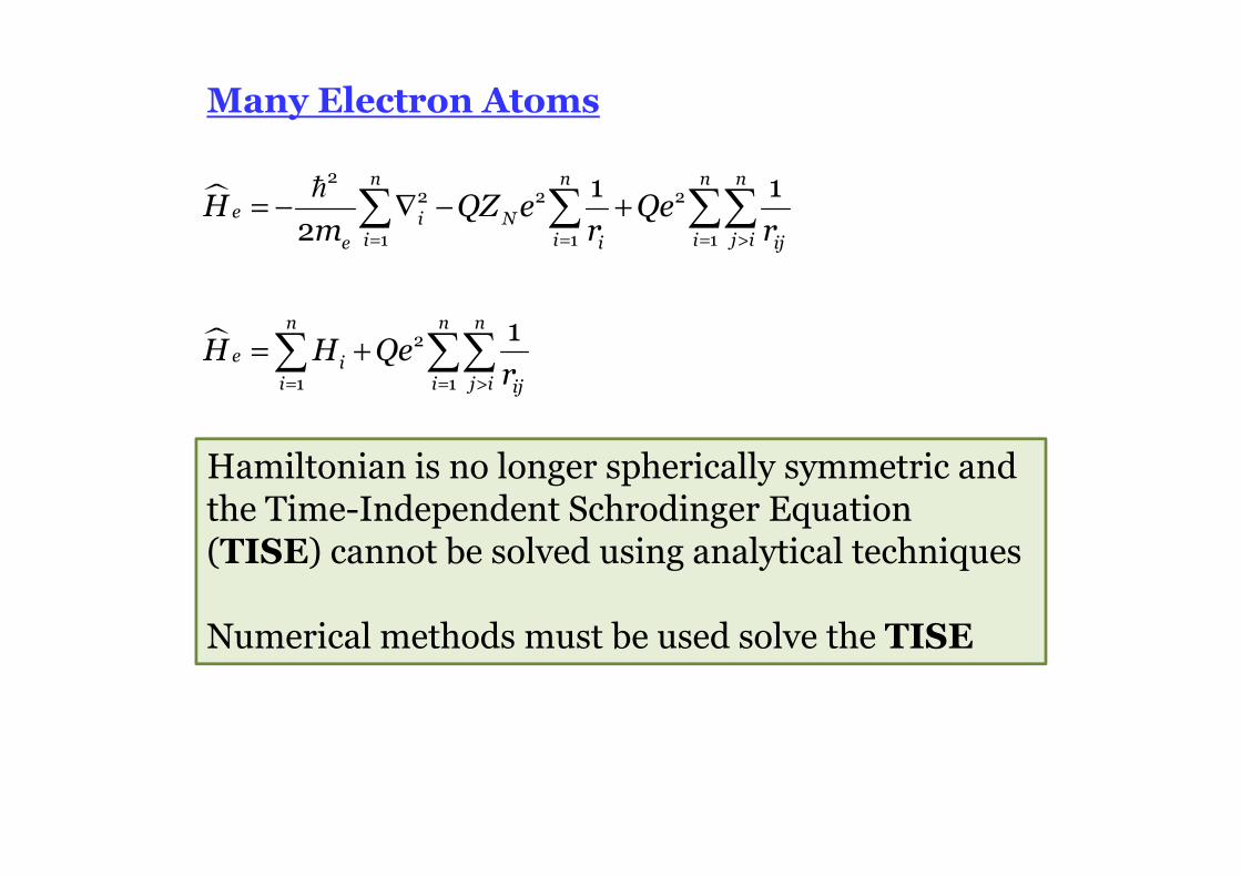
H QZ e Qem m r r
Nuclei are static
�
�
= = = >
= = >
= − ∇ − +
= +
∑ ∑ ∑∑
∑ ∑∑
�2
2 2 2
1 1 1
2
1 1
1 1
2
1
n n n n
e i Ni i i j ie i ij
n n n
e ii i j i ij
H QZ e Qem r r
H H Qer
Inter-electron repulsion term leads to deviation from the hydrogen atom. Unfortunately CANNOT be ignored
≠ +
1 1 1
ij i j
f g hr r r
term in the Hamiltonian is not separable1
ijr
Many Electron Atoms
�
�
= = = >
= = >
= − ∇ − +
= +
∑ ∑ ∑∑
∑ ∑∑
�2
2 2 2
1 1 1
2
1 1
1 1
2
1
n n n n
e i Ni i i j ie i ij
n n n
e ii i j i ij
H QZ e Qem r r
H H Qer
Hamiltonian is no longer spherically symmetric and the Time-Independent Schrodinger Equation (TISE) cannot be solved using analytical techniques
Numerical methods must be used solve the TISE
Many Electron Atoms: Orbital Approximation
He atom result indicate that neglecting the inter-electron interaction is not a good idea
Improvement
The term in the Hamiltonian represents the interaction
between the electrons. Which mean the electron move in the potential provided by the nucleus and rest of the electron.
Since the electron and nucleus have opposite charges, it can be thought that the rest of the electrons reduce the charge felt by a particular electron ⇒ Shielding
1
ijr
ψ φ φ φ φ≈ ⋅ ⋅ ⋅⋅⋅ ⋅⋅(1,2,3,... ) (1) (2) (3) ( )e n n
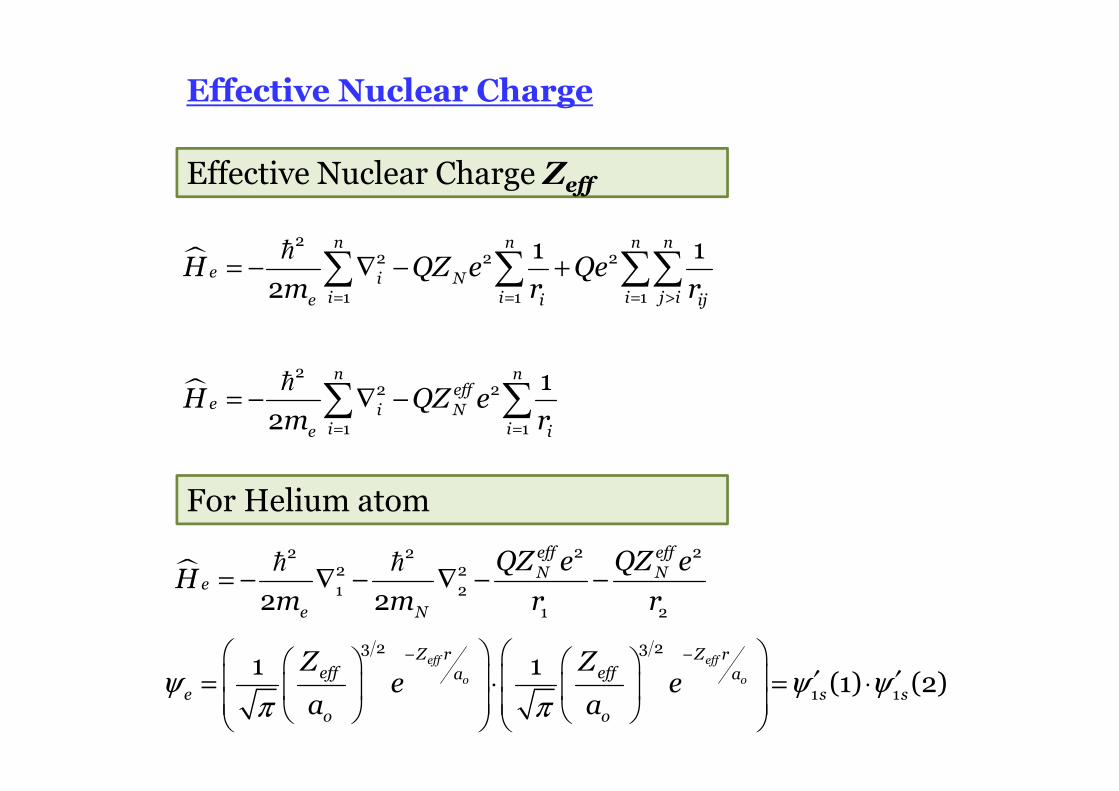
Effective Nuclear Charge
�
�
= = = >
= =
= − ∇ − +
= − ∇ −
∑ ∑ ∑∑
∑ ∑
�
�
22 2 2
1 1 1
22 2
1 1
1 12
12
n n n n
e i Ni i i j ie i ij
n neff
e i Ni ie i
H QZ e Qem r r
H QZ em r
Effective Nuclear Charge Zeff
For Helium atom
ψ ψ ψπ π
− − ′ ′= ⋅ = ⋅
3 2 3 2
1 1
1 1(1) (2)
eff eff
o o
Z r Z reff effa a
e s so o
Z Ze e
a a
� = − ∇ − ∇ − −� �
2 22 22 21 2
1 22 2
eff effN N
e
e N
QZ e QZ eH
m m r r
Effective Nuclear Charge
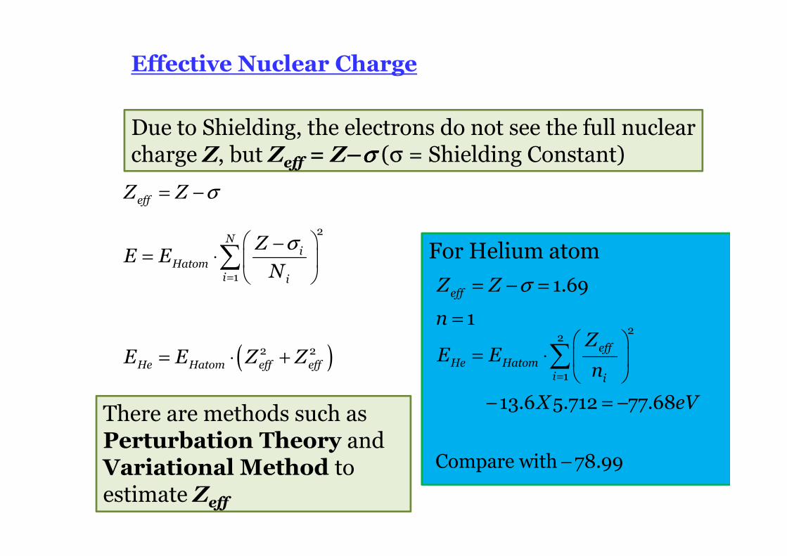
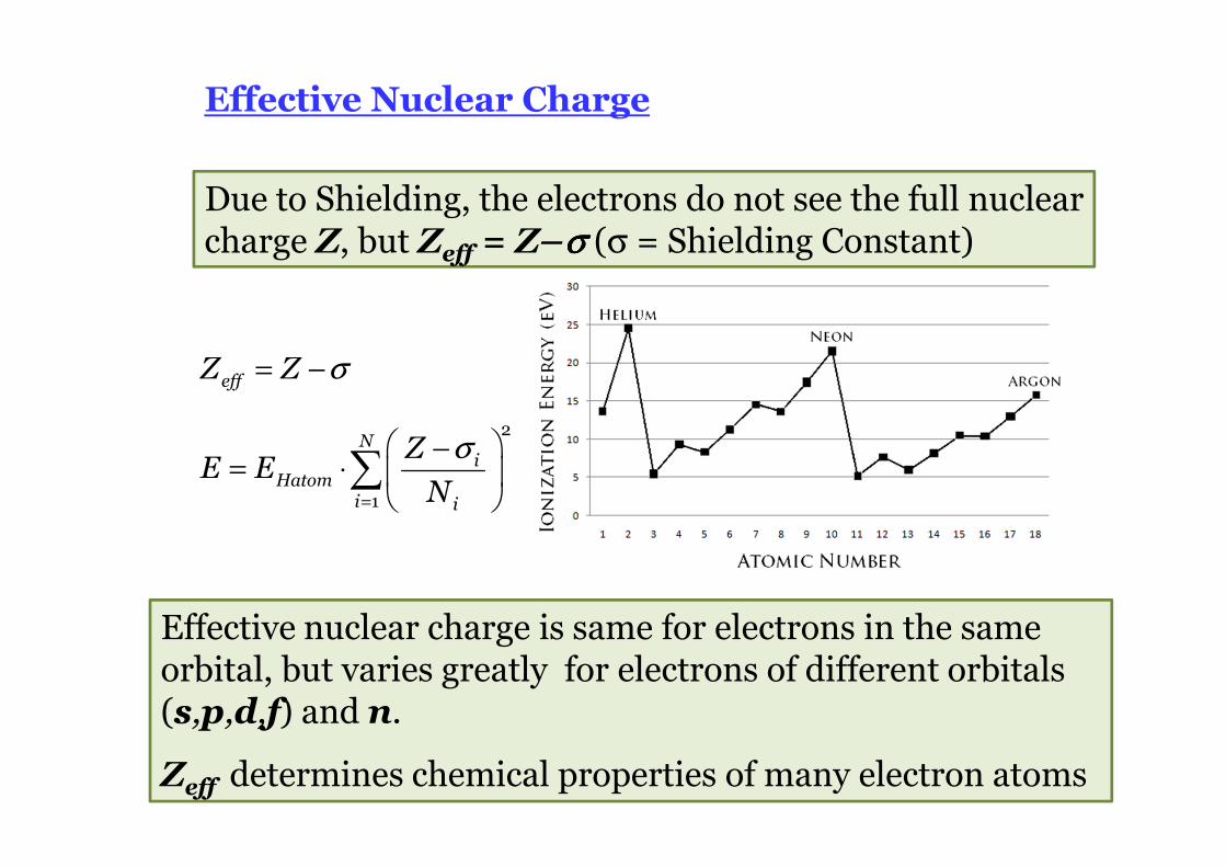
Due to Shielding, the electrons do not see the full nuclear charge Z, but Zeff = Z–σσσσ (σ = Shielding Constant)
( )
σ
σ
=
= −
−= ⋅
= ⋅ +
∑2
1
2 2
eff
Ni
Hatomi i
He Hatom eff eff
Z Z
ZE E
N
E E Z Z
For Helium atom
σ= − =
=
1.69
1
effZ Z
n
=
= ⋅
− = −
−
∑2
2
1
13.6 5.712 77.68
Compare with 78.99
effHe Hatom
i i
ZE E
n
X eVThere are methods such as Perturbation Theory and Variational Method to estimate Zeff
Effective Nuclear Charge
Due to Shielding, the electrons do not see the full nuclear charge Z, but Zeff = Z–σσσσ (σ = Shielding Constant)
σ
σ
=
= −
−= ⋅
∑
2
1
eff
Ni
Hatomi i
Z Z
ZE E
N
Effective nuclear charge is same for electrons in the same orbital, but varies greatly for electrons of different orbitals(s,p,d,f) and n.
Zeff determines chemical properties of many electron atoms
Building-up (Aufbau) Principle
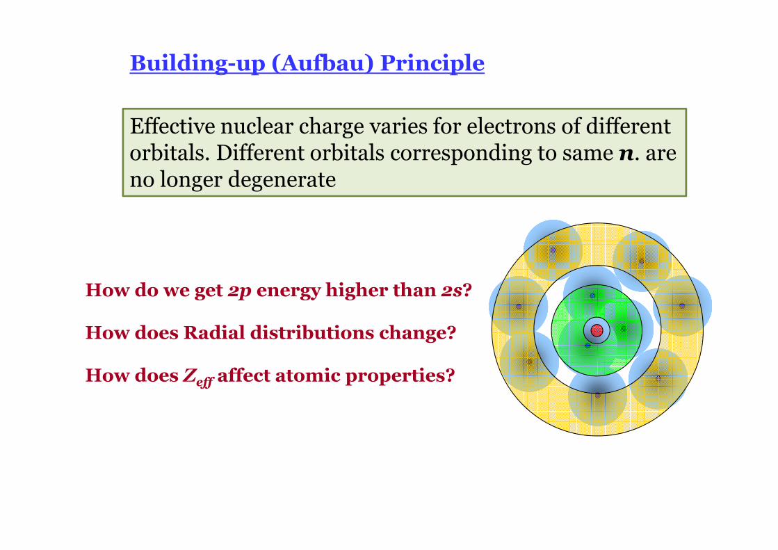
Effective nuclear charge varies for electrons of different orbitals. Different orbitals corresponding to same n. are no longer degenerate
How do we get 2p energy higher than 2s?
How does Radial distributions change?
How does Zeff affect atomic properties?
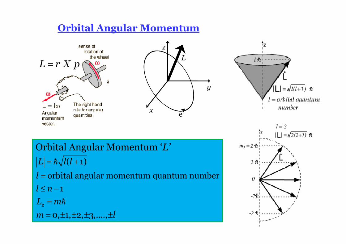
Orbital Angular Momentum
e-x
y
z
L= L r X p
Orbital Angular Momentum ‘L’
= +
=
≤ −
=
= ± ± ± ±
�
�
( 1)
orbital angular momentum quantum number
1
0, 1, 2, 3,....,z
L l l
l
l n
L m
m l
Spin Angular Momentum
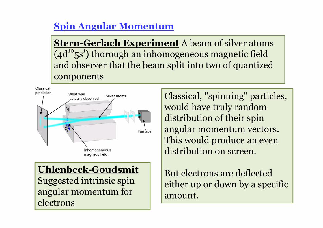
Stern-Gerlach Experiment A beam of silver atoms (4d105s1) thorough an inhomogeneous magnetic field and observer that the beam split into two of quantized components
Classical, "spinning" particles, would have truly random distribution of their spin angular momentum vectors. This would produce an even distribution on screen.
But electrons are deflected either up or down by a specific amount.
Uhlenbeck-GoudsmitSuggested intrinsic spin angular momentum for electrons
Spin Angular Momentum
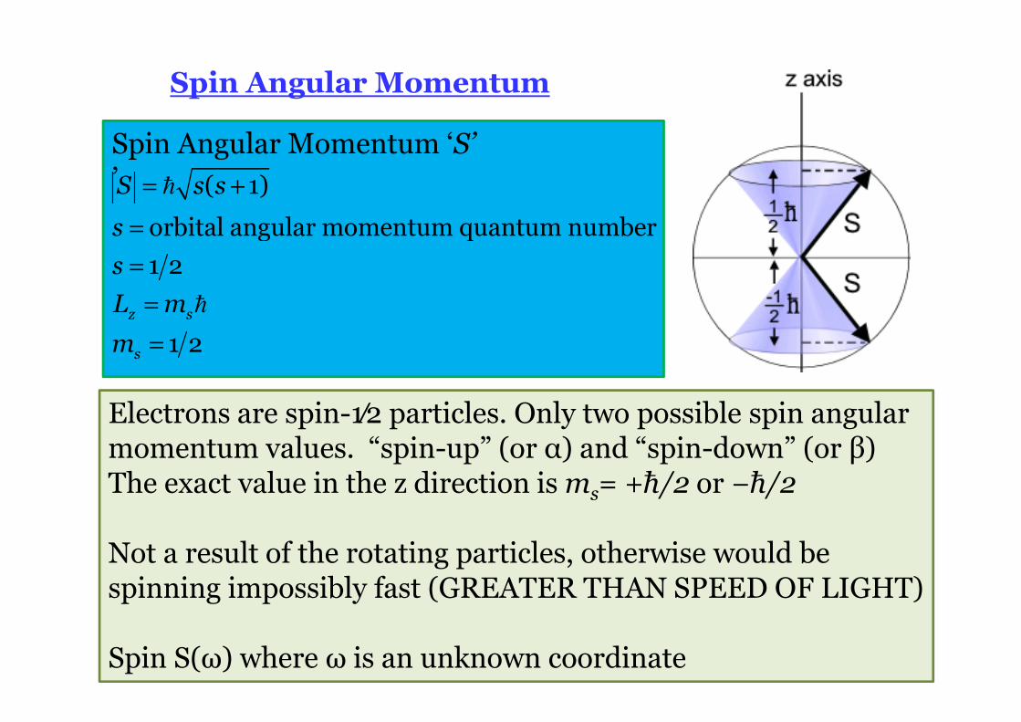
Spin Angular Momentum ‘S’’ = +
=
=
=
=
�
�
( 1)
orbital angular momentum quantum number
1 2
1 2z s
s
S s s
s
s
L m
m
Electrons are spin-1⁄2 particles. Only two possible spin angular momentum values. “spin-up” (or α) and “spin-down” (or β)The exact value in the z direction is ms= +ħ/2 or −ħ/2
Not a result of the rotating particles, otherwise would be spinning impossibly fast (GREATER THAN SPEED OF LIGHT)
Spin S(ω) where ω is an unknown coordinate
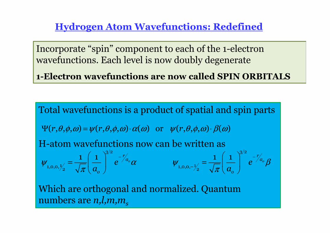
Hydrogen Atom Wavefunctions: Redefined
Incorporate “spin” component to each of the 1-electron wavefunctions. Each level is now doubly degenerate
1-Electron wavefunctions are now called SPIN ORBITALS
Total wavefunctions is a product of spatial and spin parts
H-atom wavefunctions now can be written as
Which are orthogonal and normalized. Quantum numbers are n,l,m,ms
θ φ ω ψ θ φ ω α ω ψ θ φ ω β ω
ψ α ψ βπ π
− −
−
Ψ = ⋅ ⋅
= =
3 2 3 2
1 11,0,0, 1,0,0,2 2
( , , , ) ( , , , ) ( ) or ( , , , ) ( )
1 1 1 1 o o
r ra a
o o
r r r
e ea a
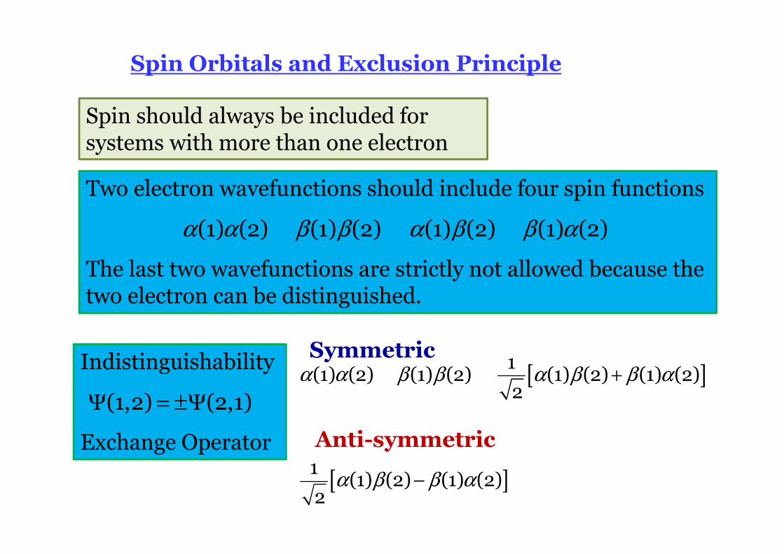
Spin Orbitals and Exclusion Principle
Spin should always be included for systems with more than one electron
Two electron wavefunctions should include four spin functions
The last two wavefunctions are strictly not allowed because the two electron can be distinguished.
α α β β α β β α(1) (2) (1) (2) (1) (2) (1) (2)
Indistinguishability
Exchange Operator
Ψ = ±Ψ(1,2) (2,1)[ ]
[ ]
α α β β α β β α
α β β α
+
−
1(1) (2) (1) (2) (1) (2) (1) (2)
2
1(1) (2) (1) (2)
2
Symmetric
Anti-symmetric
He atom wavefunction
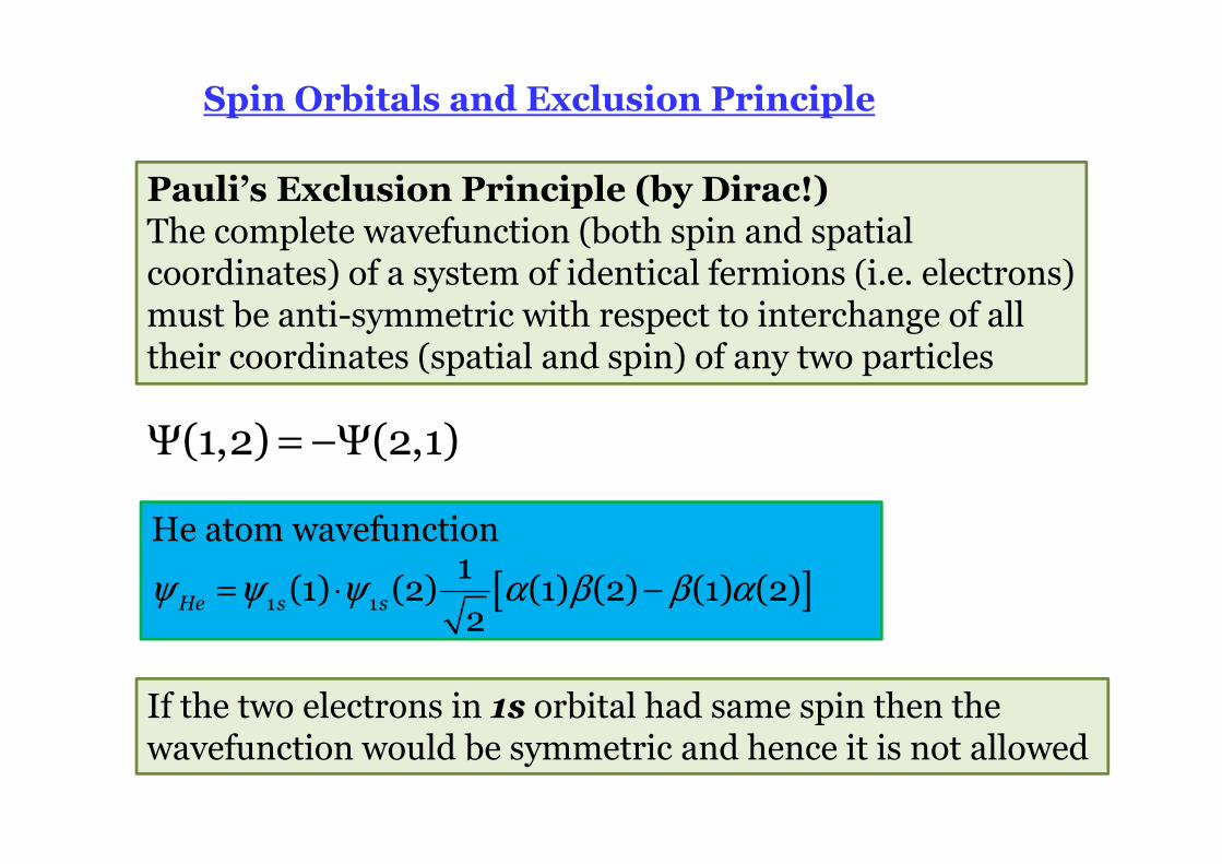
Spin Orbitals and Exclusion Principle
Ψ = −Ψ(1,2) (2,1)
[ ]ψ ψ ψ α β β α= ⋅ −1 1
1(1) (2) (1) (2) (1) (2)
2He s s
Pauli’s Exclusion Principle (by Dirac!)The complete wavefunction (both spin and spatial coordinates) of a system of identical fermions (i.e. electrons) must be anti-symmetric with respect to interchange of all their coordinates (spatial and spin) of any two particles
If the two electrons in 1s orbital had same spin then the wavefunction would be symmetric and hence it is not allowed
Helium Atom: Excited States
[ ] [ ]
α α
α β β α
β β
= =
⋅ − ⋅ + = = = = −
(1) (2) ( 1; 1)
1 11 (1) 2 (2) 1 (2) 2 (1) (1) (2) (1) (2) ( 1; 0)
2 2(1) (2) ( 1; 1)
s
s
s
s m
s s s s s m
s m
[ ][ ]α β β α⋅ + ⋅ − = =1 1
1 (1) 2 (2) 1 (2) 2 (1) (1) (2) (1) (2) ( 0; 0)2 2
ss s s s s m
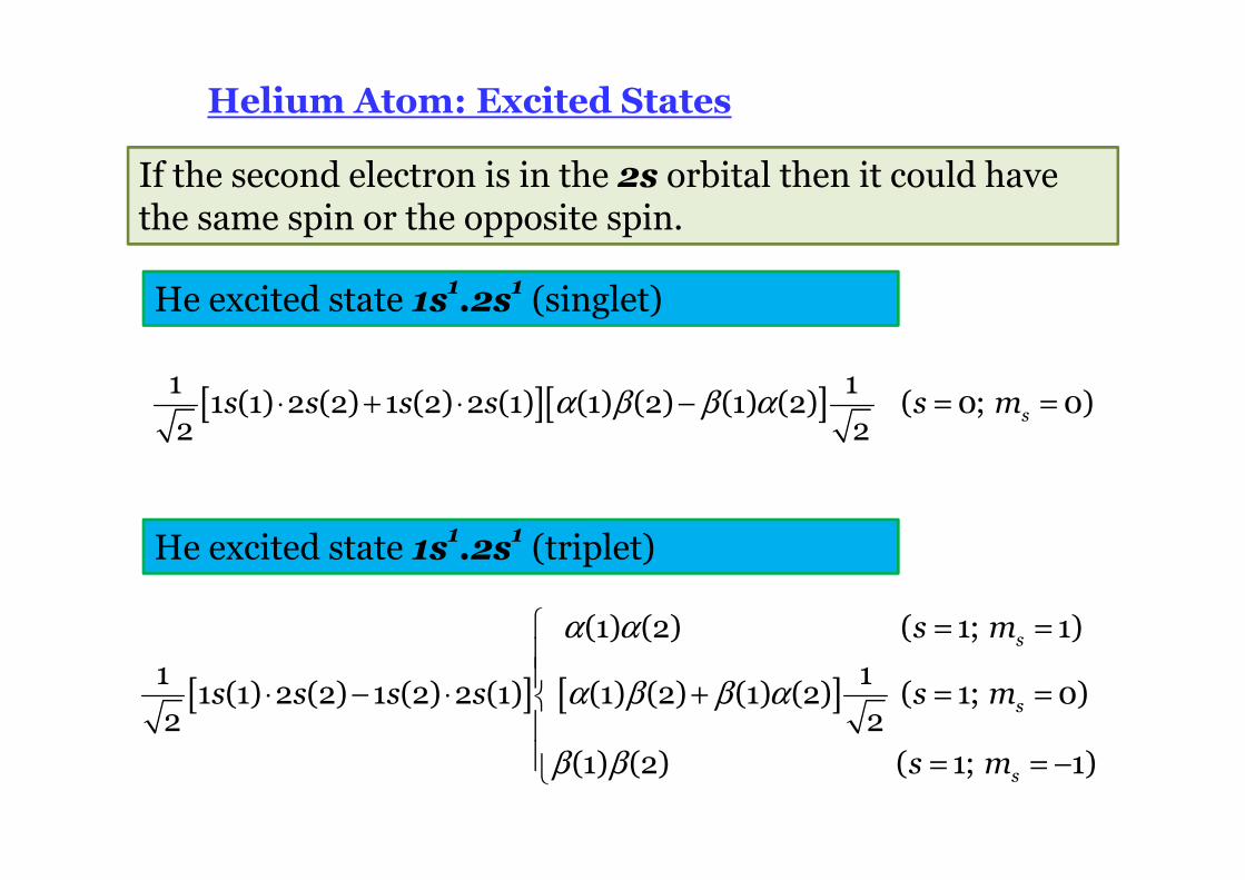
If the second electron is in the 2s orbital then it could have the same spin or the opposite spin.
He excited state 1s1.2s1 (triplet)
He excited state 1s1.2s1 (singlet)
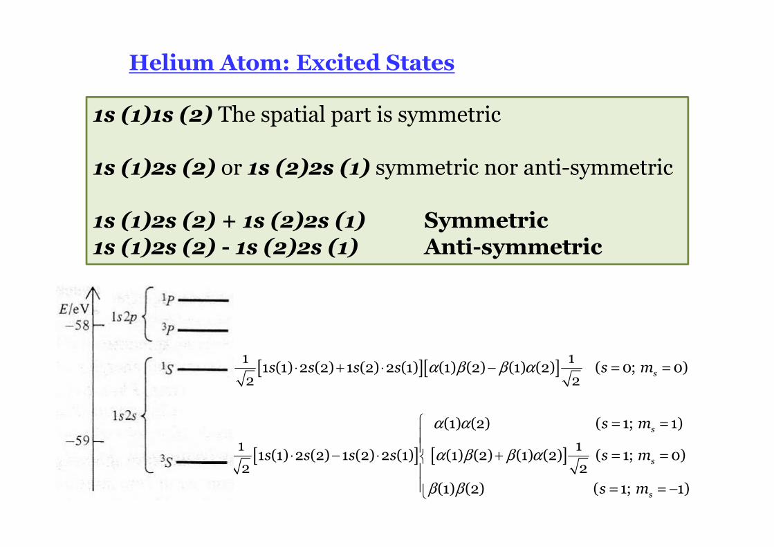
1s (1)1s (2) The spatial part is symmetric
1s (1)2s (2) or 1s (2)2s (1) symmetric nor anti-symmetric
1s (1)2s (2) + 1s (2)2s (1) Symmetric1s (1)2s (2) - 1s (2)2s (1) Anti-symmetric
[ ] [ ]
α α
α β β α
β β
= =
⋅ − ⋅ + = = = = −
(1) (2) ( 1; 1)
1 11 (1) 2 (2) 1 (2) 2 (1) (1) (2) (1) (2) ( 1; 0)
2 2(1) (2) ( 1; 1)
s
s
s
s m
s s s s s m
s m
[ ][ ]α β β α⋅ + ⋅ − = =1 1
1 (1) 2 (2) 1 (2) 2 (1) (1) (2) (1) (2) ( 0; 0)2 2
ss s s s s m
Helium Atom: Excited States
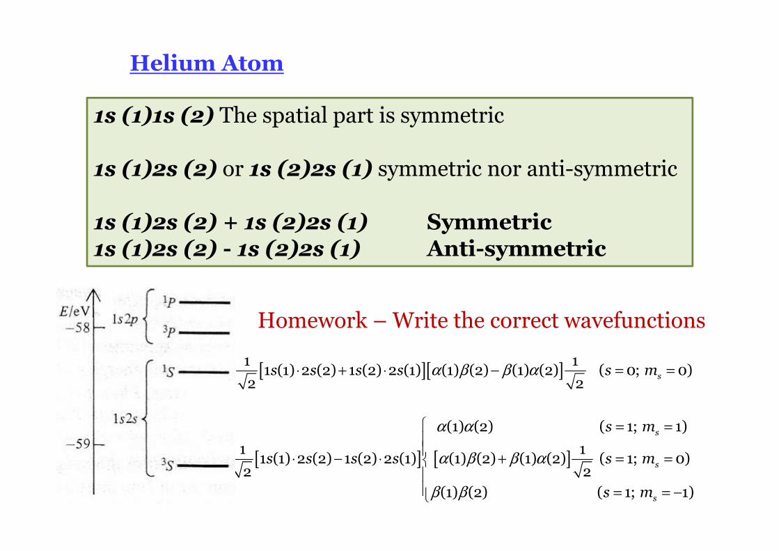
Helium Atom
1s (1)1s (2) The spatial part is symmetric
1s (1)2s (2) or 1s (2)2s (1) symmetric nor anti-symmetric
1s (1)2s (2) + 1s (2)2s (1) Symmetric1s (1)2s (2) - 1s (2)2s (1) Anti-symmetric
[ ] [ ]
α α
α β β α
β β
= =
⋅ − ⋅ + = = = = −
(1) (2) ( 1; 1)
1 11 (1) 2 (2) 1 (2) 2 (1) (1) (2) (1) (2) ( 1; 0)
2 2(1) (2) ( 1; 1)
s
s
s
s m
s s s s s m
s m
[ ][ ]α β β α⋅ + ⋅ − = =1 1
1 (1) 2 (2) 1 (2) 2 (1) (1) (2) (1) (2) ( 0; 0)2 2
ss s s s s m
Homework – Write the correct wavefunctions
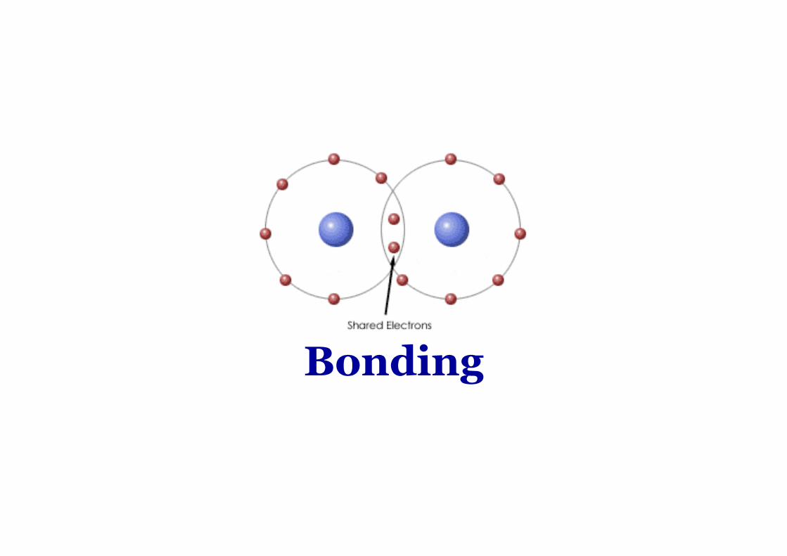
Bonding
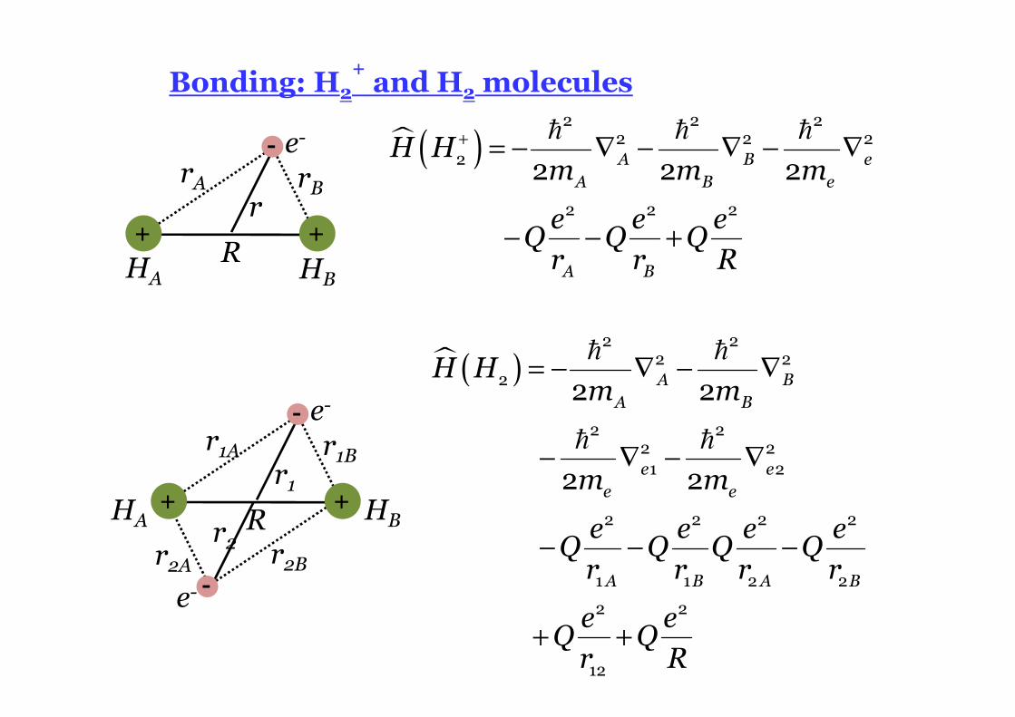
Bonding: H2
+and H2molecules
+
-
+RHA HB
rA rBr
e-
+
-
+RHA HB
r1A r1Br1
e-
-e-r2Br2A
r2
� ( )+ = − ∇ − ∇ − ∇
− − +
� � �2 2 2
2 2 22
2 2 2
2 2 2
A B eA B e
A B
H Hm m m
e e eQ Q Qr r R
� ( ) = − ∇ − ∇
− ∇ − ∇
− − −
+ +
� �
� �
2 22 2
2
2 22 21 2
2 2 2 2
1 1 2 2
2 2
12
2 2
2 2
A BA B
e ee e
A B A B
H Hm m
m m
e e e eQ Q Q Qr r r r
e eQ Qr R
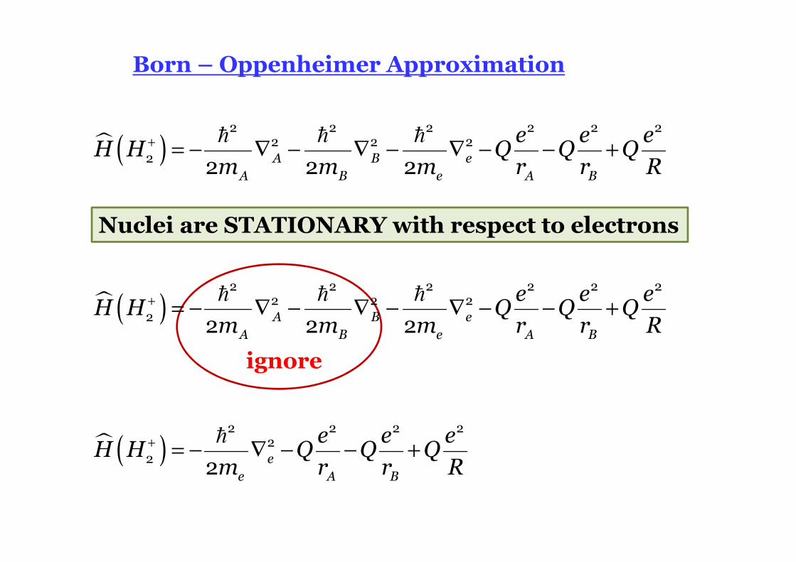
Born – Oppenheimer Approximation
� ( )+ = − ∇ − ∇ − ∇ − − +� � �2 2 2 2 2 2
2 2 22 2 2 2A B e
A B e A B
e e eH H Q Q Q
m m m r r R
Nuclei are STATIONARY with respect to electrons
� ( )+ = − ∇ − − +�2 2 2 2
22 2 e
e A B
e e eH H Q Q Q
m r r R
� ( )+ = − ∇ − ∇ − ∇ − − +� � �2 2 2 2 2 2
2 2 22 2 2 2A B e
A B e A B
e e eH H Q Q Q
m m m r r R
ignore
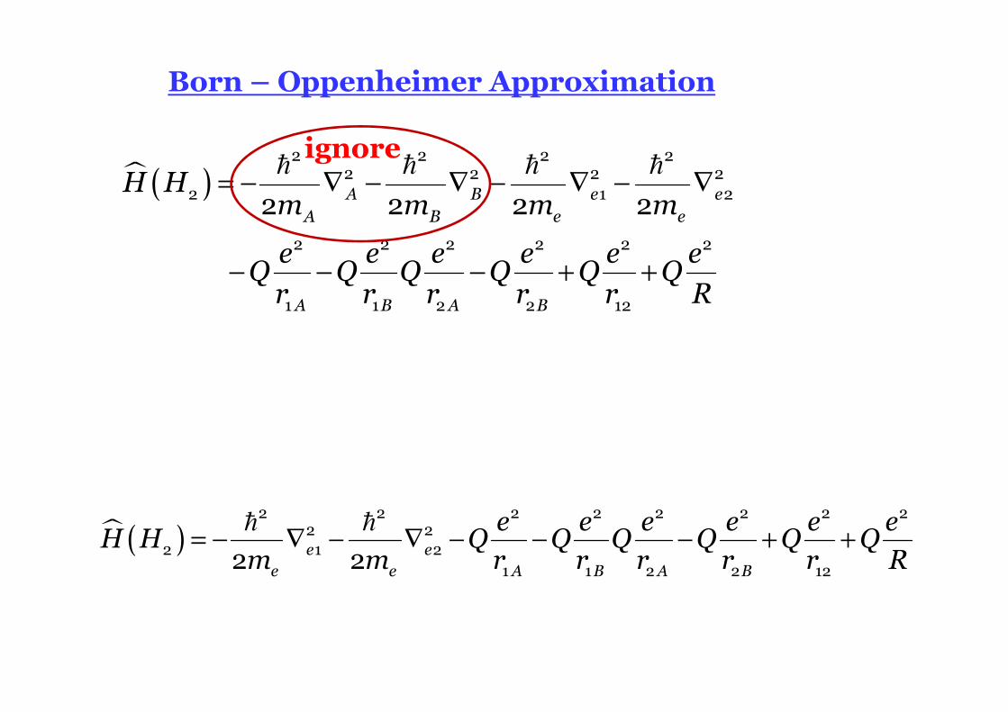
Born – Oppenheimer Approximation
� ( ) = − ∇ − ∇ − ∇ − ∇
− − − + +
� � � �2 2 2 2
2 2 2 22 1 2
2 2 2 2 2 2
1 1 2 2 12
2 2 2 2
A B e eA B e e
A B A B
H Hm m m m
e e e e e eQ Q Q Q Q Qr r r r r R
� ( ) = − ∇ − ∇ − − − + +� �2 2 2 2 2 2 2 2
2 22 1 2
1 1 2 2 122 2e ee e A B A B
e e e e e eH H Q Q Q Q Q Q
m m r r r r r R
ignore
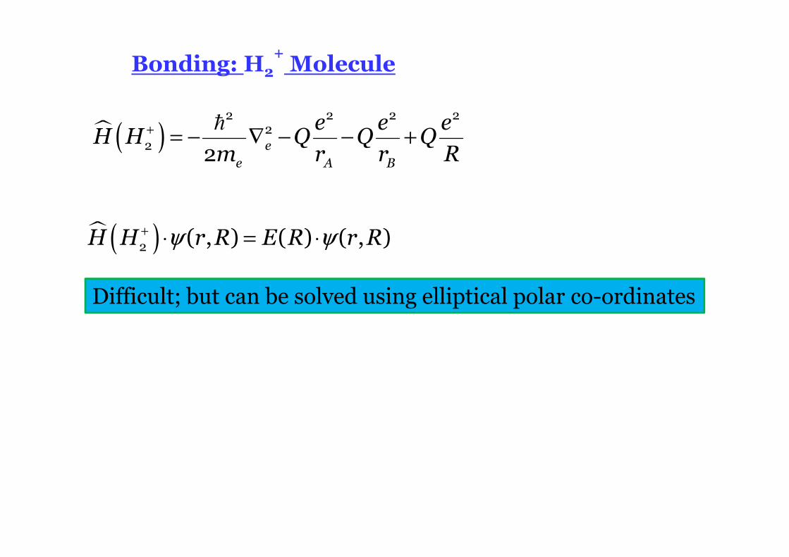
Bonding: H2
+Molecule
� ( )+ = − ∇ − − +�2 2 2 2
22 2 e
e A B
e e eH H Q Q Q
m r r R
� ( ) ψ ψ+ ⋅ = ⋅2 ( , ) ( ) ( , )H H r R E R r R
Difficult; but can be solved using elliptical polar co-ordinates
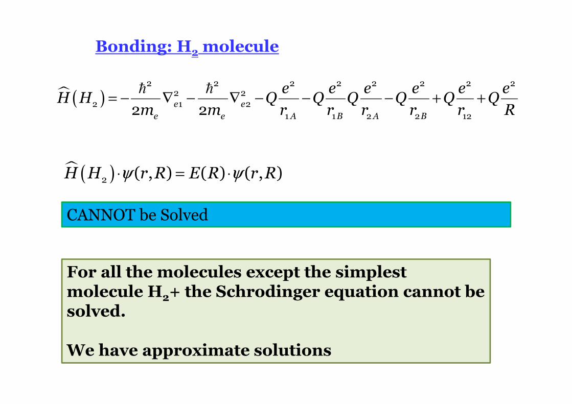
Bonding: H2molecule
� ( ) ψ ψ⋅ = ⋅2 ( , ) ( ) ( , )H H r R E R r R
CANNOT be Solved
� ( ) = − ∇ − ∇ − − − + +� �2 2 2 2 2 2 2 2
2 22 1 2
1 1 2 2 122 2e ee e A B A B
e e e e e eH H Q Q Q Q Q Q
m m r r r r r R
For all the molecules except the simplest molecule H2+ the Schrodinger equation cannot be solved.
We have approximate solutions
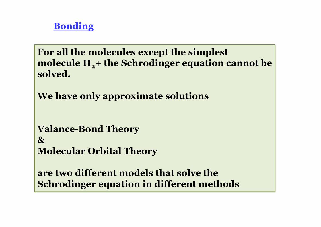
Bonding
For all the molecules except the simplest molecule H2+ the Schrodinger equation cannot be solved.
We have only approximate solutions
Valance-Bond Theory & Molecular Orbital Theory
are two different models that solve the Schrodinger equation in different methods
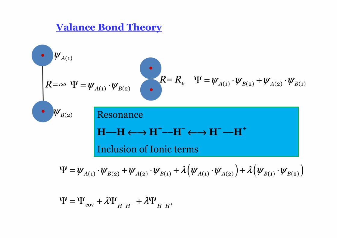
Valance Bond Theory
ψ ψΨ = ⋅(1) (2)A Bψ ψ ψ ψΨ = ⋅ + ⋅(1) (2) (2) (1)A B A B
ψ (1)A
ψ (2)B
R=∞ R= Re
( ) ( )ψ ψ ψ ψ λ ψ ψ λ ψ ψ
λ λ+ − − +
Ψ = ⋅ + ⋅ + ⋅ + ⋅
Ψ = Ψ + Ψ + Ψ
(1) (2) (2) (1) (1) (2) (1) (2)
cov
A B A B A A B B
H H H H
Resonance
H−−−−−−−−H ←→←→←→←→ H+−−−−−−−−H
−−−−←→←→←→←→ H
−−−−−−−−−−−−H
+
Inclusion of Ionic terms
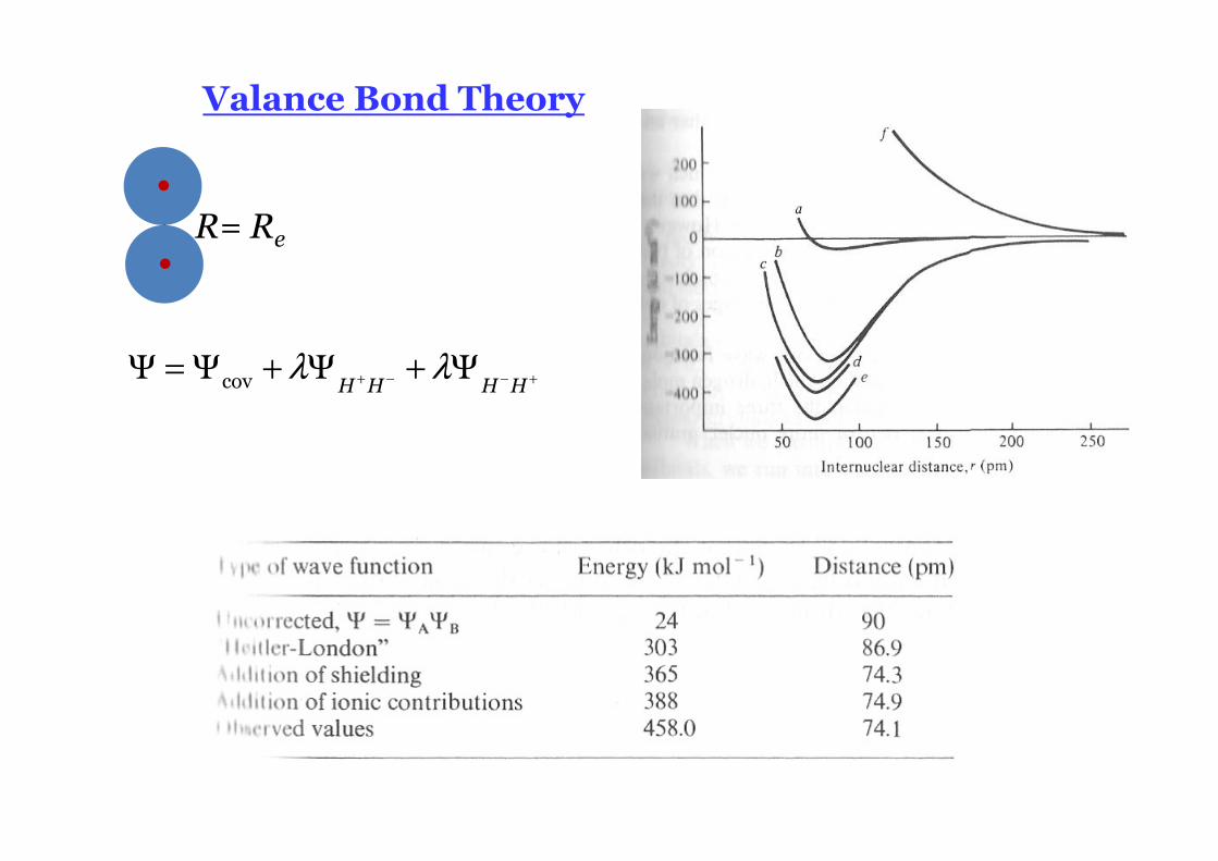
Valance Bond Theory
R= Re
λ λ+ − − +Ψ = Ψ + Ψ + Ψcov H H H H
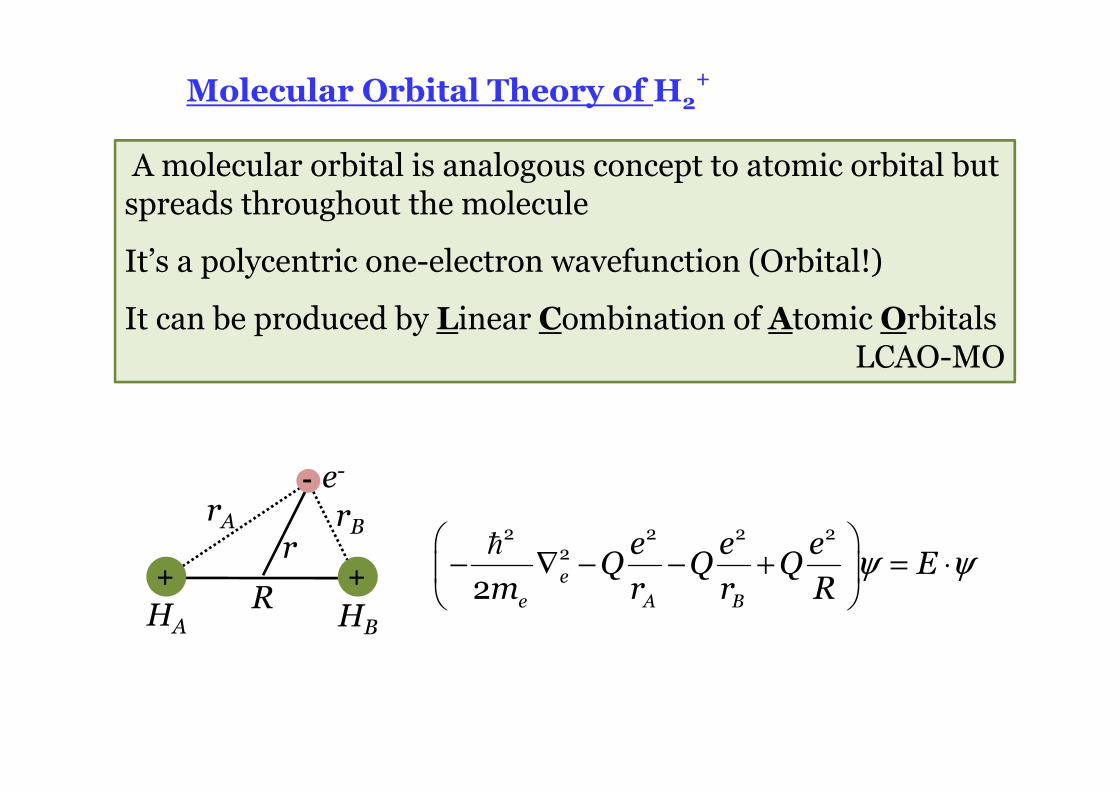
+
-
+RHA HB
rA rBr
e-
A molecular orbital is analogous concept to atomic orbital but spreads throughout the molecule
It’s a polycentric one-electron wavefunction (Orbital!)
It can be produced by Linear Combination of Atomic OrbitalsLCAO-MO
ψ ψ
− ∇ − − + = ⋅
�2 2 2 2
2
2 ee A B
e e eQ Q Q E
m r r R
Molecular Orbital Theory of H2+
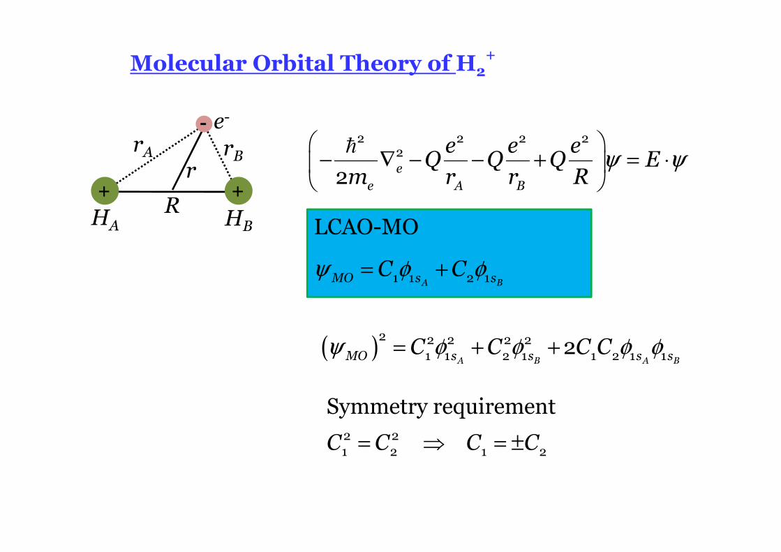
+
-
+RHA HB
rA rBr
e-
ψ ψ
− ∇ − − + = ⋅
�2 2 2 2
2
2 ee A B
e e eQ Q Q E
m r r R
LCAO-MO
ψ φ φ= +1 1 2 1A BMO s sC C
( )ψ φ φ φ φ= + +2 2 2 2 2
1 1 2 1 1 2 1 12A B A BMO s s s sC C C C
= ⇒ = ±2 21 2 1 2
Symmetry requirement
C C C C
Molecular Orbital Theory of H2+
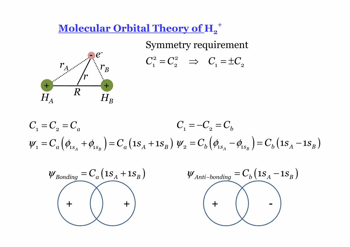
+
-
+RHA HB
rA rBr
e-= ⇒ = ±2 2
1 2 1 2
Symmetry requirement
C C C C
( ) ( )ψ φ φ
= =
= + = +
1 2
1 1 1 1 1A B
a
a s s a A B
C C C
C C s s ( ) ( )ψ φ φ
= − =
= − = −
1 2
2 1 1 1 1A B
b
b s s b A B
C C C
C C s s
+ +
( )ψ = +1 1Bonding a A BC s s
+ -
( )ψ − = −1 1Anti bonding b A BC s s
Molecular Orbital Theory of H2+
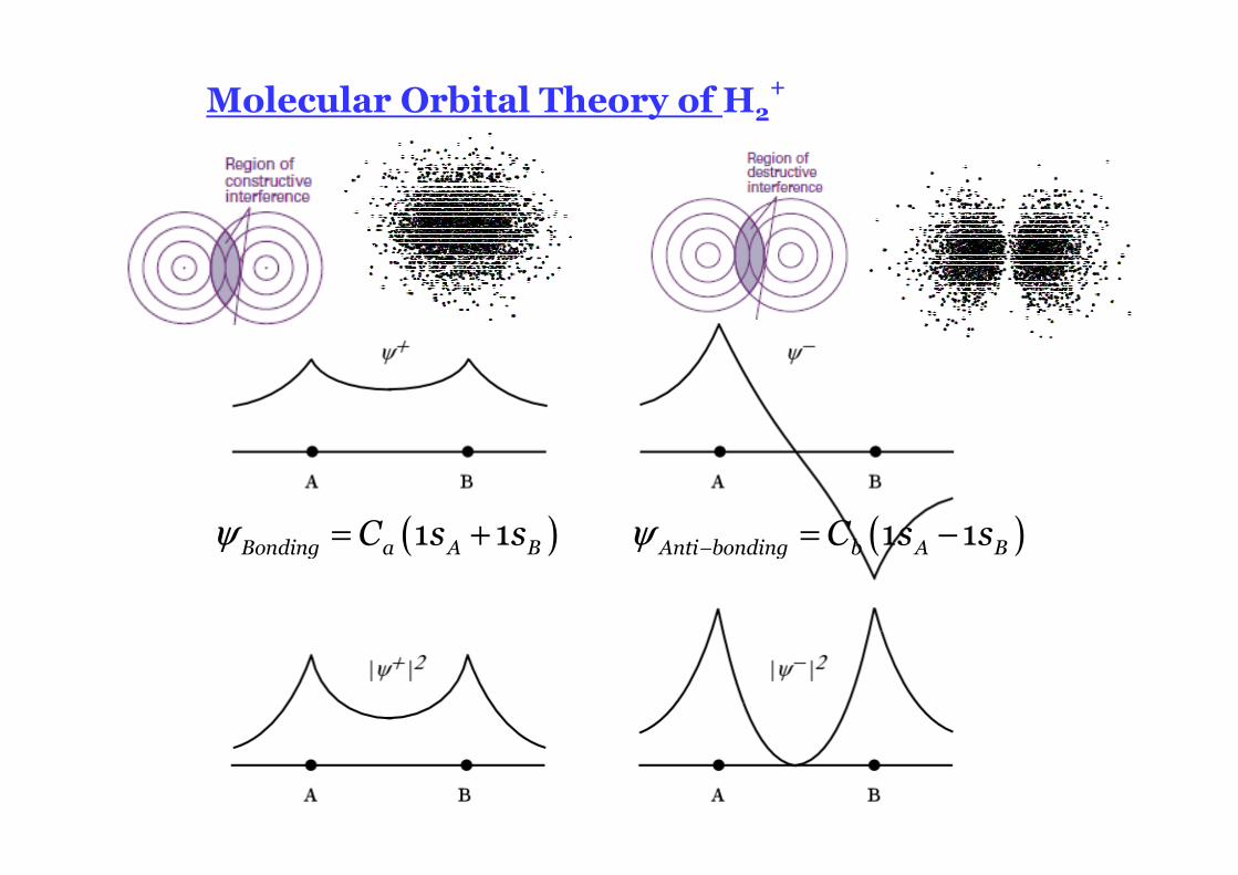
( )ψ = +1 1Bonding a A BC s s ( )ψ − = −1 1Anti bonding b A BC s s
Molecular Orbital Theory of H2+
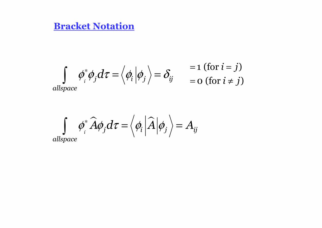
Bracket Notation
� �
φ φ τ φ φ δ
φ φ τ φ φ
∗
∗
= =
= =
∫
∫
i
i
j i j ijallspace
j i j ijallspace
d
A d A A
= =
= ≠
1 (for )
0 (for )
i j
i j
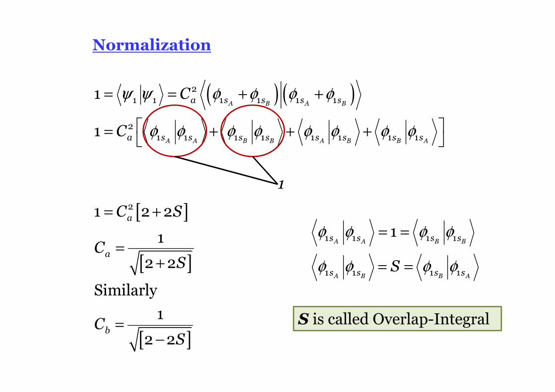
Normalization
( ) ( )
[ ]
[ ]
[ ]
ψ ψ φ φ φ φ
φ φ φ φ φ φ φ φ
= = + +
= + + +
= +
=+
=−
21 1 1 1 1 1
21 1 1 1 1 1 1 1
2
1
1
1 2 2
1
2 2
Similarly
1
2 2
A B A B
A A B B A B B A
a s s s s
a s s s s s s s s
a
a
b
C
C
C S
CS
CS
1
S is called Overlap-Integral
φ φ φ φ
φ φ φ φ
= =
= =
1 1 1 1
1 1 1 1
1A A B B
A B B A
s s s s
s s s sS
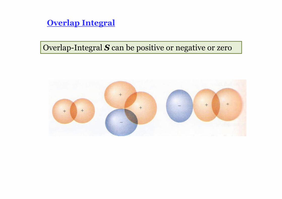
Overlap Integral
Overlap-Integral S can be positive or negative or zero
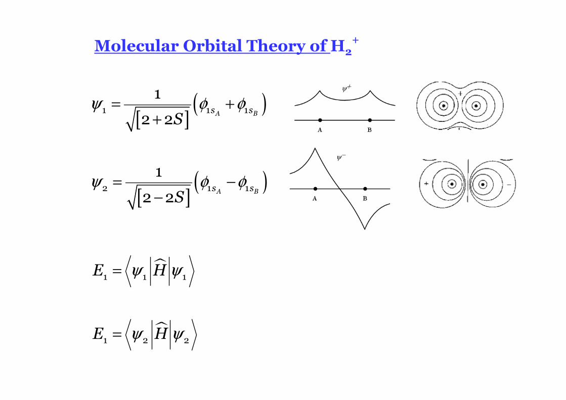
[ ]( )
[ ]( )
ψ φ φ
ψ φ φ
= ++
= −−
1 1 1
2 1 1
1
2 2
1
2 2
A B
A B
s s
s s
S
S
�
�
ψ ψ
ψ ψ
=
=
1 1 1
1 2 2
E H
E H
Molecular Orbital Theory of H2+
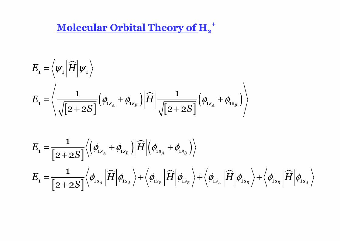
�
[ ]( ) �
[ ]( )
[ ]( ) � ( )
[ ]� � � �
ψ ψ
φ φ φ φ
φ φ φ φ
φ φ φ φ φ φ φ φ
=
= + ++ +
= + ++
= + + ++
1 1 1
1 1 1 1 1
1 1 1 1 1
1 1 1 1 1 1 1 1 1
1 1
2 2 2 2
1
2 2
1
2 2
A B A B
A B A B
A A B B A B B A
s s s s
s s s s
s s s s s s s s
E H
E HS S
E HS
E H H H HS
Molecular Orbital Theory of H2+
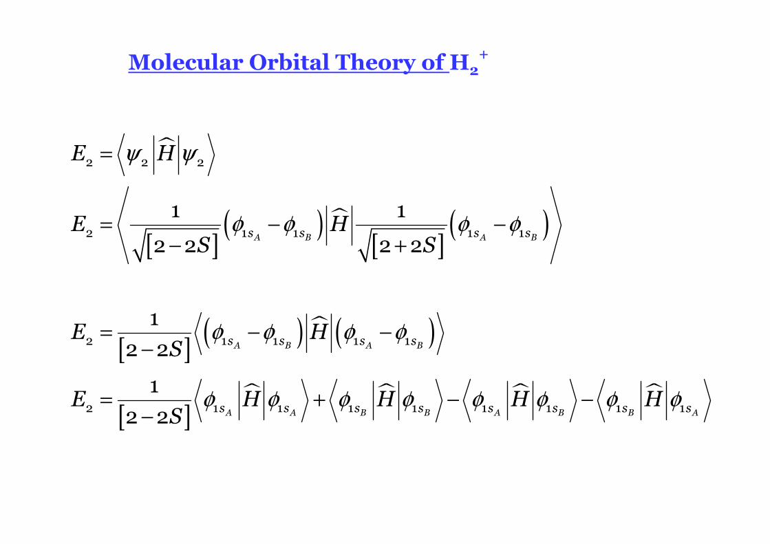
�
[ ]( ) �
[ ]( )
[ ]( ) � ( )
[ ]� � � �
ψ ψ
φ φ φ φ
φ φ φ φ
φ φ φ φ φ φ φ φ
=
= − −− +
= − −−
= + − −−
2 2 2
2 1 1 1 1
2 1 1 1 1
2 1 1 1 1 1 1 1 1
1 1
2 2 2 2
1
2 2
1
2 2
A B A B
A B A B
A A B B A B B A
s s s s
s s s s
s s s s s s s s
E H
E HS S
E HS
E H H H HS
Molecular Orbital Theory of H2+
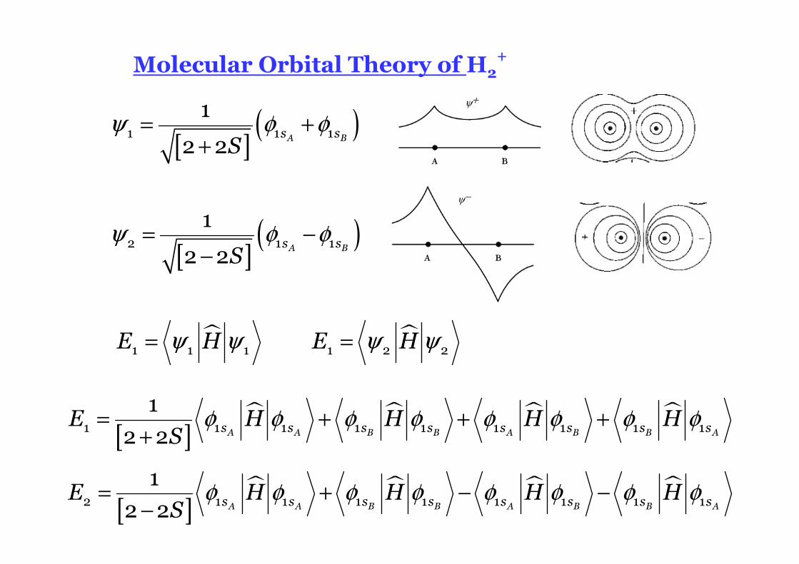
[ ]( )
[ ]( )
ψ φ φ
ψ φ φ
= ++
= −−
1 1 1
2 1 1
1
2 2
1
2 2
A B
A B
s s
s s
S
S
� �ψ ψ ψ ψ= =1 1 1 1 2 2 E H E H
Molecular Orbital Theory of H2+
[ ]� � � �φ φ φ φ φ φ φ φ= + − −
−2 1 1 1 1 1 1 1 1
1
2 2 A A B B A B B As s s s s s s sE H H H HS
[ ]� � � �φ φ φ φ φ φ φ φ= + + +
+1 1 1 1 1 1 1 1 1
1
2 2 A A B B A B B As s s s s s s sE H H H HS
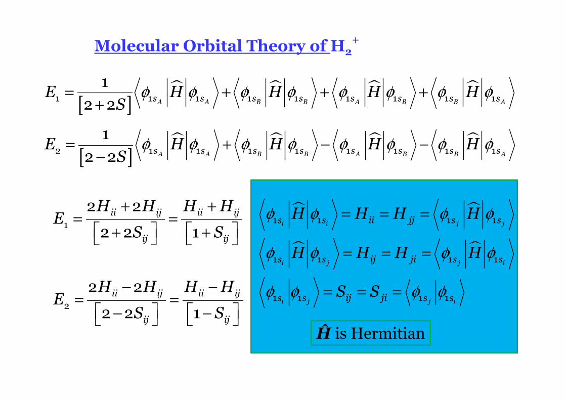
[ ]� � � �φ φ φ φ φ φ φ φ= + + +
+1 1 1 1 1 1 1 1 1
1
2 2 A A B B A B B As s s s s s s sE H H H HS
Molecular Orbital Theory of H2+
� �
� �
φ φ φ φ
φ φ φ φ
φ φ φ φ
= = =
= = =
= = =
1 1 1 1
1 1 1 1
1 1 1 1
i i j j
i j j i
i j j i
s s ii jj s s
s s ij ji s s
s s ij ji s s
H H H H
H H H H
S S
Ĥ is Hermitian
[ ]� � � �φ φ φ φ φ φ φ φ= + − −
−2 1 1 1 1 1 1 1 1
12 2 A A B B A B B As s s s s s s sE H H H H
S
+ += =
+ +
− −= =
− −
1
2
2 2
2 2 1
2 2
2 2 1
ii ij ii ij
ij ij
ii ij ii ij
ij ij
H H H HE
S S
H H H HE
S S
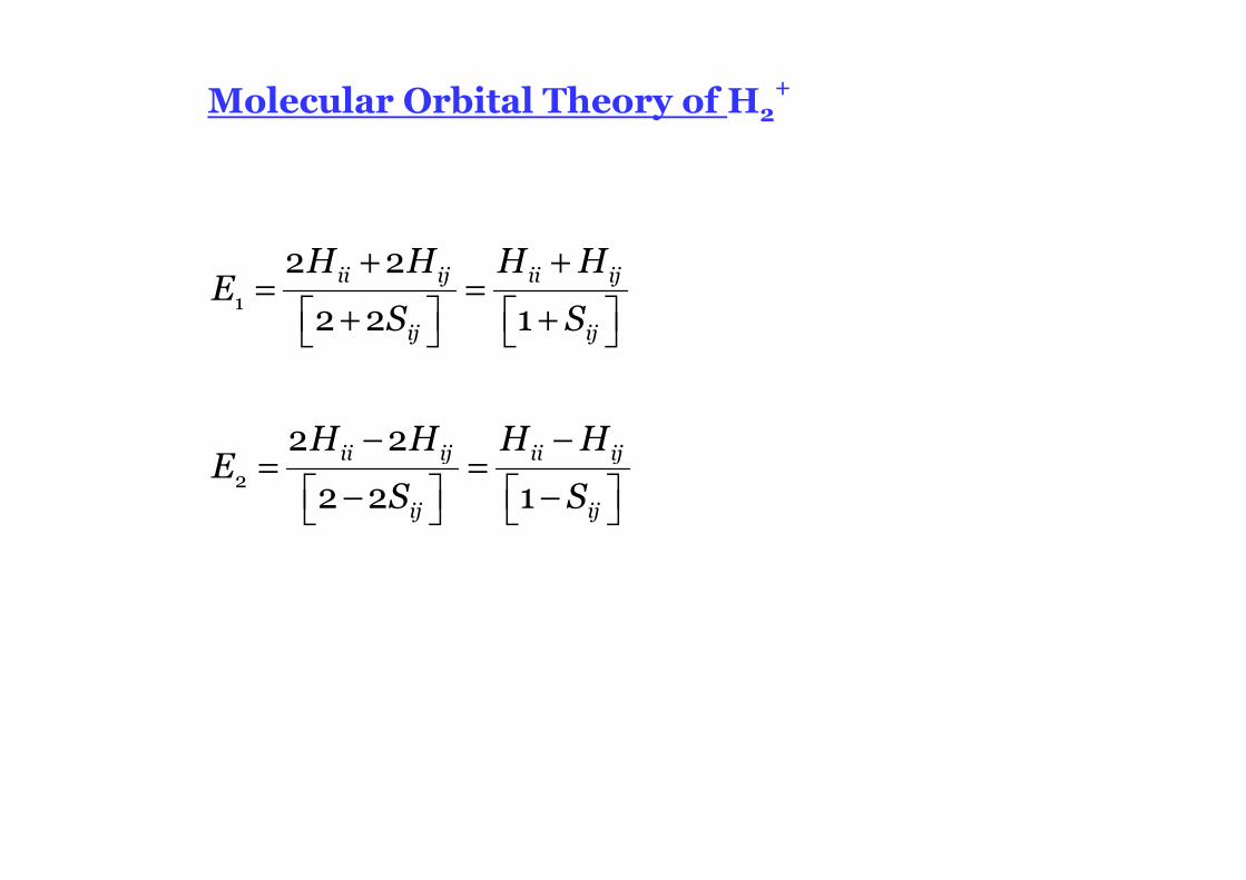
Molecular Orbital Theory of H2+
+ += =
+ +
− −= =
− −
1
2
2 2
2 2 1
2 2
2 2 1
ii ij ii ij
ij ij
ii ij ii ij
ij ij
H H H HE
S S
H H H HE
S S
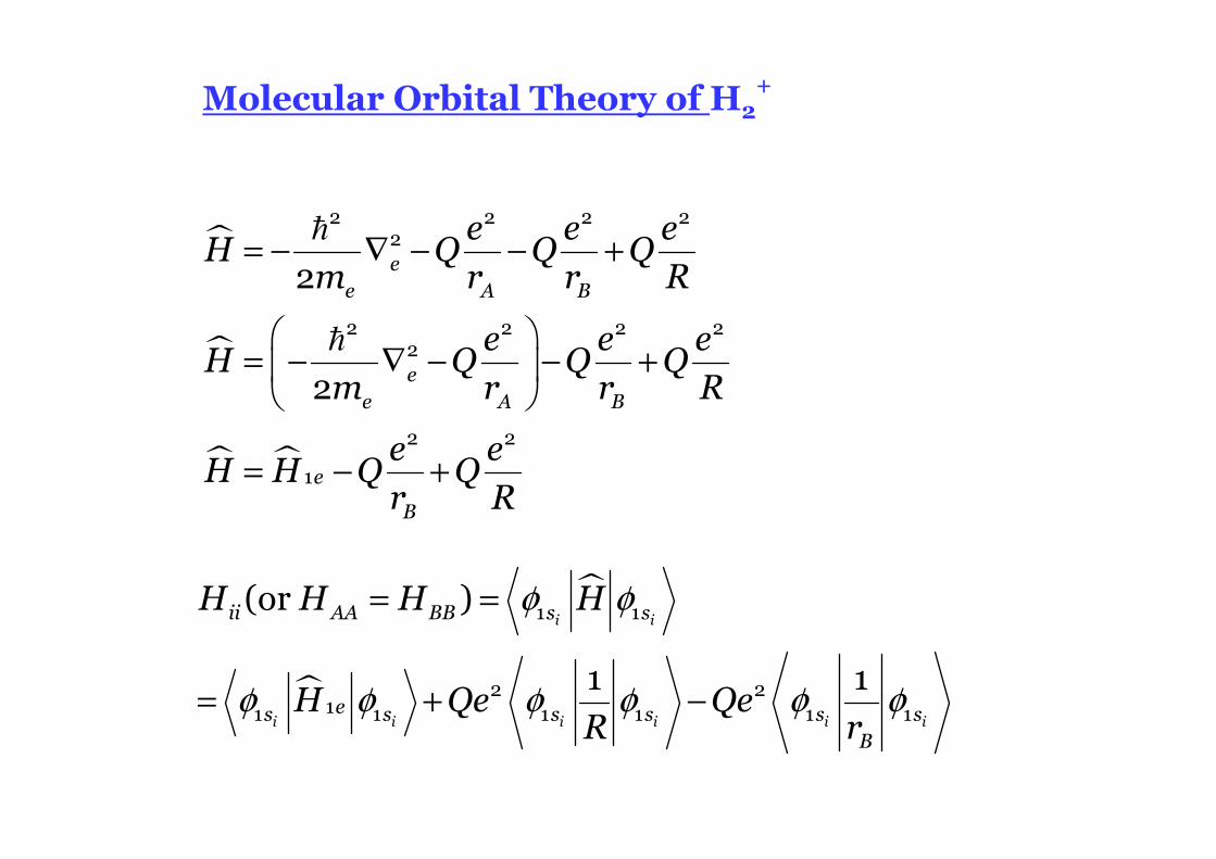
Molecular Orbital Theory of H2+
�
�
� �
= − ∇ − − +
= − ∇ − − +
= − +
�
�
2 2 2 22
2 2 2 22
2 2
1
2
2
ee A B
ee A B
e
B
e e eH Q Q Q
m r r R
e e eH Q Q Q
m r r R
e eH H Q Q
r R
�
�
φ φ
φ φ φ φ φ φ
= =
= + −
1 1
2 211 1 1 1 1 1
(or )
1 1
i i
i i i i i i
ii AA BB s s
es s s s s sB
H H H H
H Qe QeR r
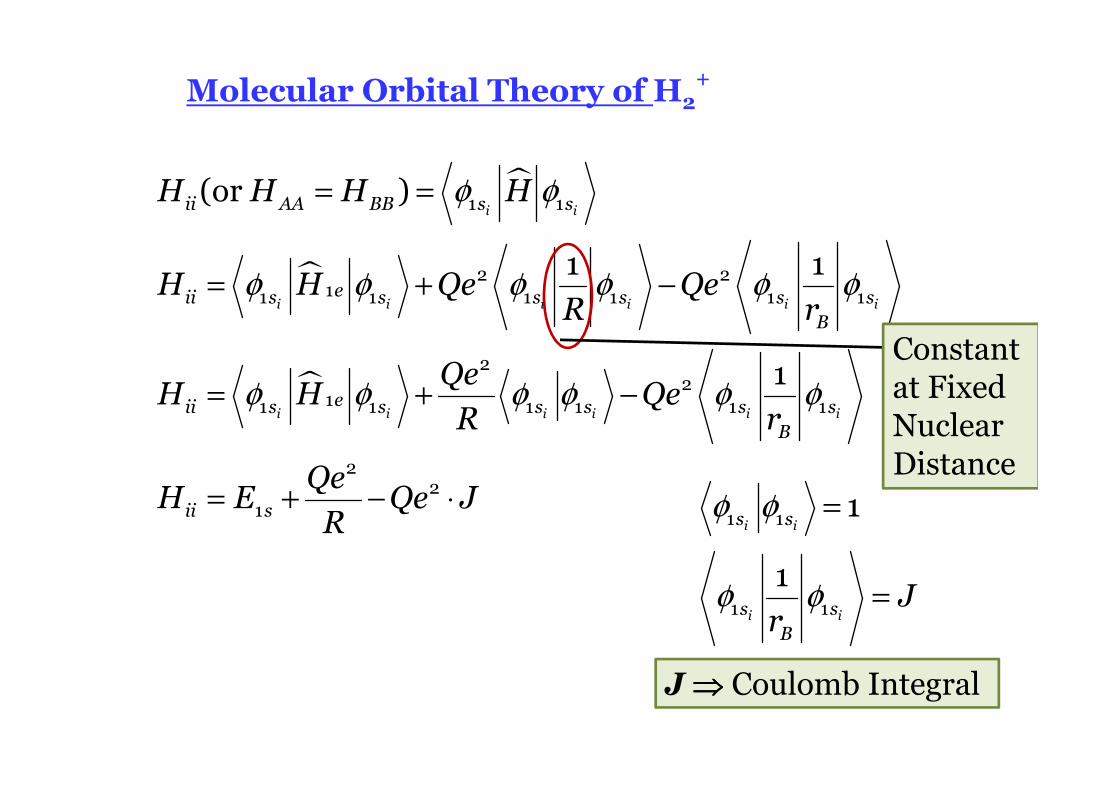
Molecular Orbital Theory of H2+
�
�
�
φ φ
φ φ φ φ φ φ
φ φ φ φ φ φ
= =
= + −
= + −
= + − ⋅
1 1
2 211 1 1 1 1 1
22
11 1 1 1 1 1
22
1
(or )
1 1
1
i i
i i i i i i
i i i i i i
ii AA BB s s
eii s s s s s sB
eii s s s s s sB
ii s
H H H H
H H Qe QeR r
QeH H Qe
R r
QeH E Qe J
R φ φ
φ φ
=
=
1 1
1 1
1
1
i i
i i
s s
s sB
Jr
Constant at Fixed Nuclear Distance
J ⇒⇒⇒⇒ Coulomb Integral
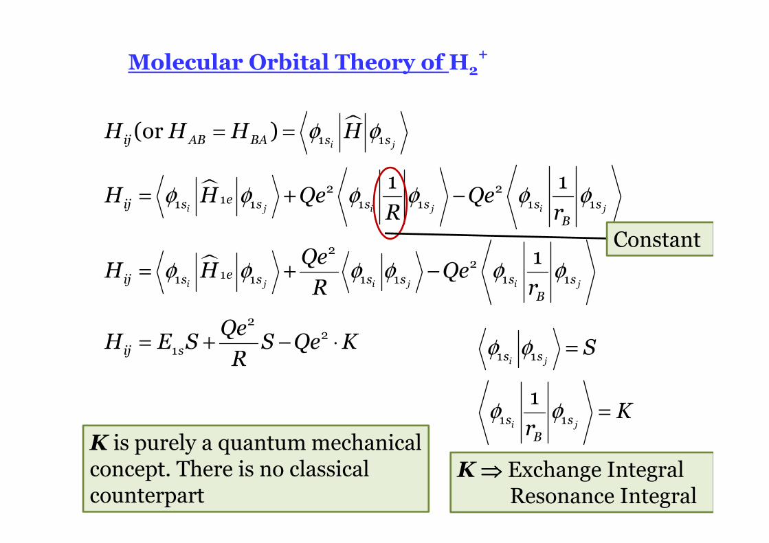
Molecular Orbital Theory of H2+
�
�
�
φ φ
φ φ φ φ φ φ
φ φ φ φ φ φ
= =
= + −
= + −
= + − ⋅
1 1
2 211 1 1 1 1 1
22
11 1 1 1 1 1
22
1
(or )
1 1
1
i j
i j i j i j
i j i j i j
ij AB BA s s
eij s s s s s sB
eij s s s s s sB
ij s
H H H H
H H Qe QeR r
QeH H Qe
R r
QeH E S S Qe K
R φ φ
φ φ
=
=
1 1
1 1
1
i j
i j
s s
s sB
S
Kr
K ⇒⇒⇒⇒ Exchange IntegralResonance Integral
Constant
K is purely a quantum mechanical concept. There is no classical counterpart
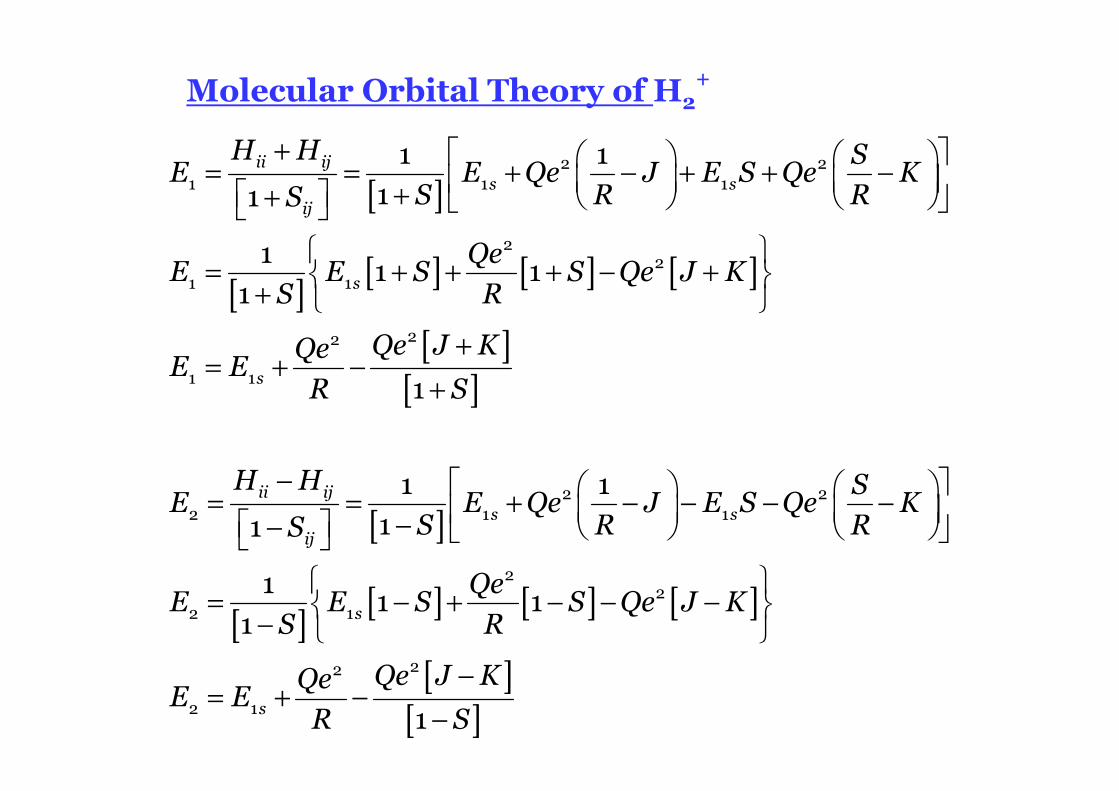
Molecular Orbital Theory of H2+
[ ]
[ ][ ] [ ] [ ]
[ ][ ]
[ ]
[ ][ ]
+ = = + − + + − + +
= + + + − +
+
+= + −
+
− = = + − − − − − −
= −−
2 21 1 1
22
1 1
22
1 1
2 22 1 1
2 1
1 1
11
11 1
1
1
1 1
11
11
1
ii ijs s
ij
s
s
ii ijs s
ij
s
H H SE E Qe J E S Qe K
S R RS
QeE E S S Qe J K
S R
Qe J KQeE E
R S
H H SE E Qe J E S Qe K
S R RS
E E SS
[ ] [ ]
[ ][ ]
+ − − −
−= + −
−
22
22
2 1
1
1s
QeS Qe J K
R
Qe J KQeE E
R S
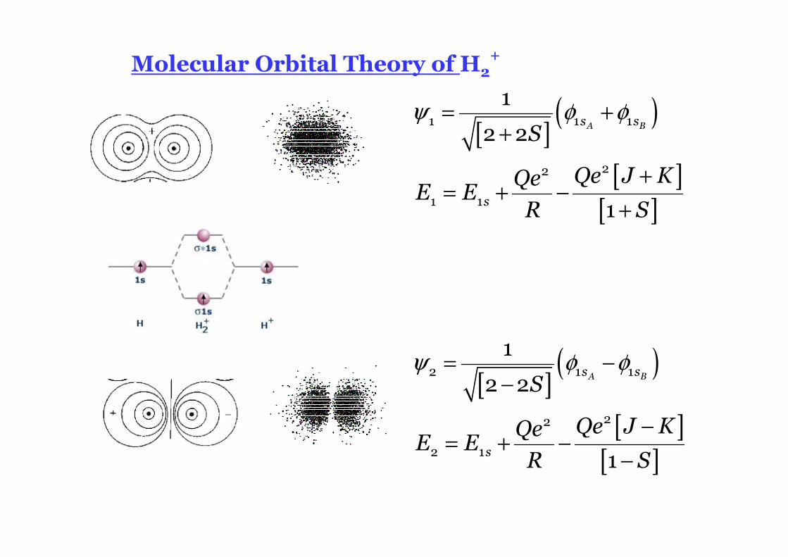
Molecular Orbital Theory of H2+
[ ]( )
[ ][ ]
[ ]( )
[ ][ ]
ψ φ φ
ψ φ φ
= ++
+= + −
+
= −−
−= + −
−
1 1 1
22
1 1
2 1 1
22
2 1
1
2 2
1
1
2 2
1
A B
A B
s s
s
s s
s
S
Qe J KQeE E
R S
S
Qe J KQeE E
R S
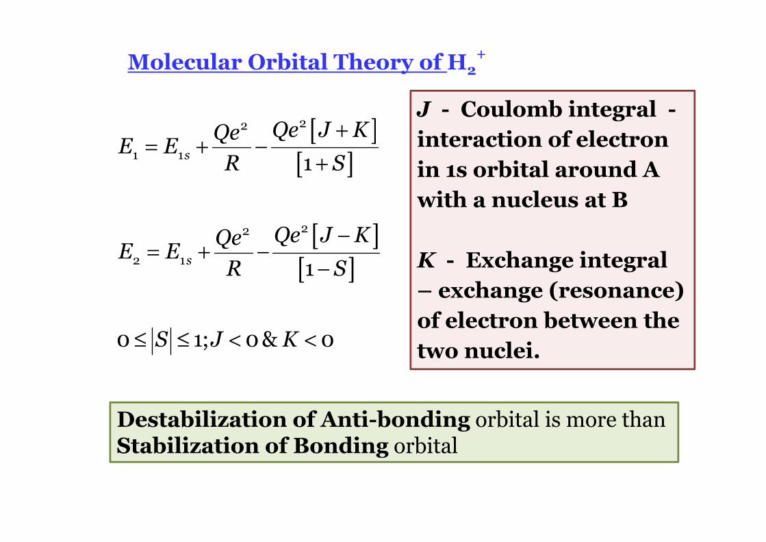
Molecular Orbital Theory of H2+
[ ][ ]
[ ][ ]
+= + −
+
−= + −
−
≤ ≤ < <
22
1 1
22
2 1
1
1
0 1; 0& 0
s
s
Qe J KQeE E
R S
Qe J KQeE E
R S
S J K
Destabilization of Anti-bonding orbital is more than Stabilization of Bonding orbital
J - Coulomb integral -
interaction of electron
in 1s orbital around A
with a nucleus at B
K - Exchange integral
– exchange (resonance)
of electron between the
two nuclei.
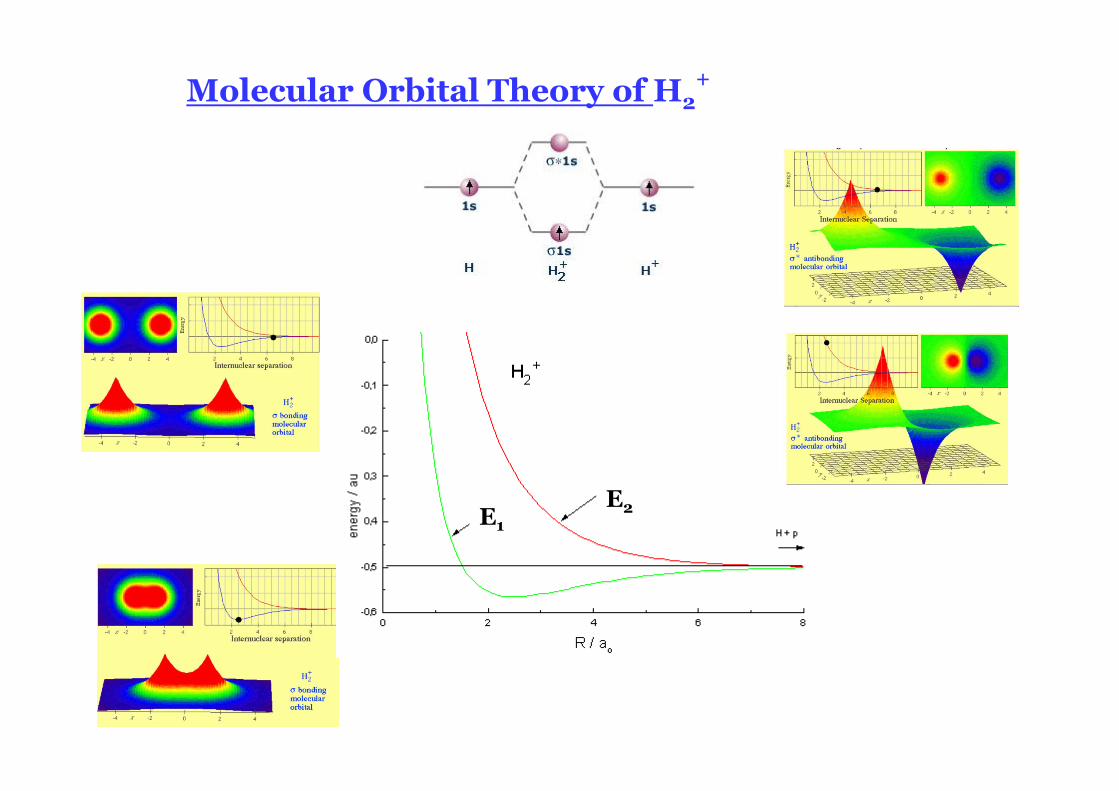
Molecular Orbital Theory of H2+
E1
1E2
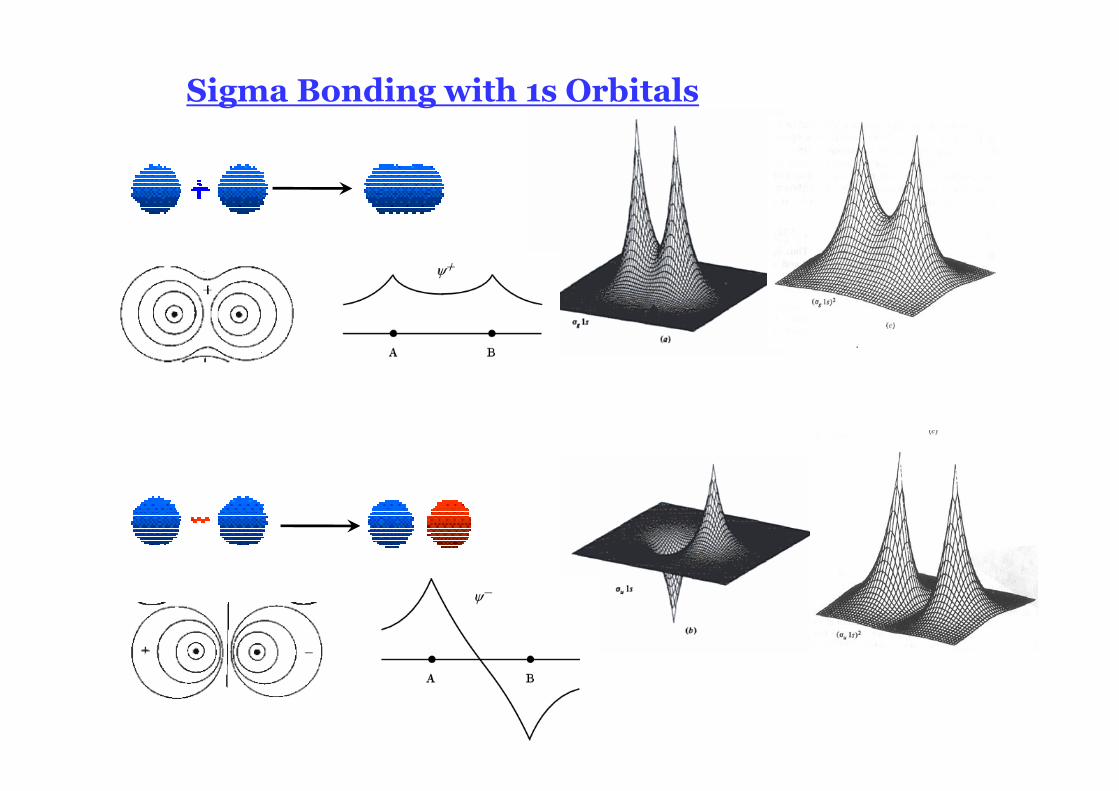
Sigma Bonding with 1s Orbitals
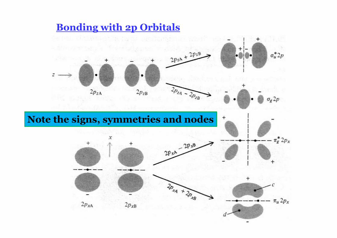
Bonding with 2p Orbitals
Note the signs, symmetries and nodes
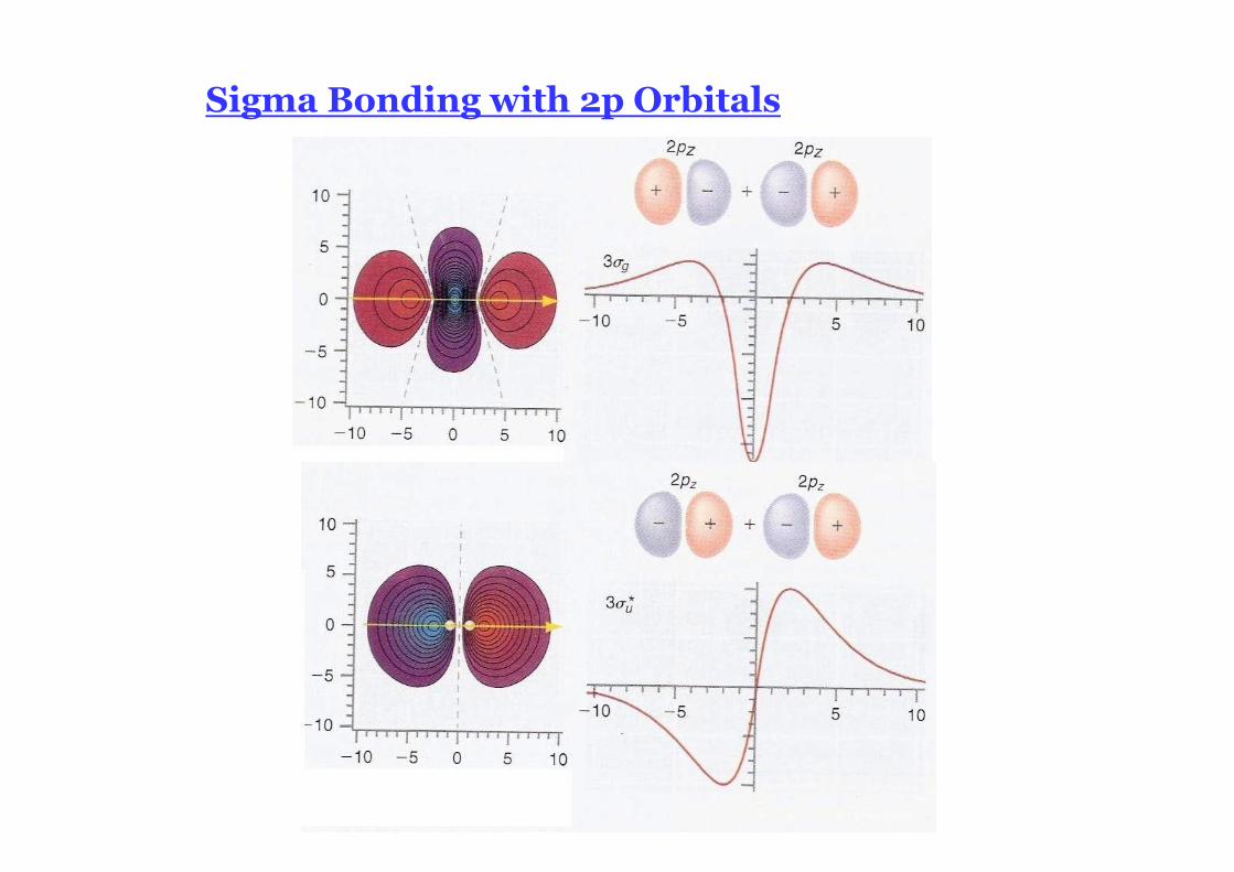
Sigma Bonding with 2p Orbitals
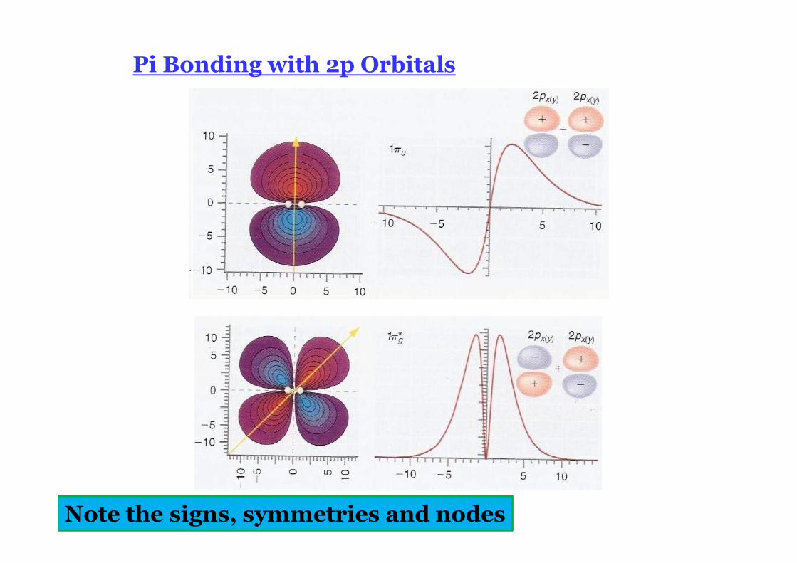
Pi Bonding with 2p Orbitals
Note the signs, symmetries and nodes
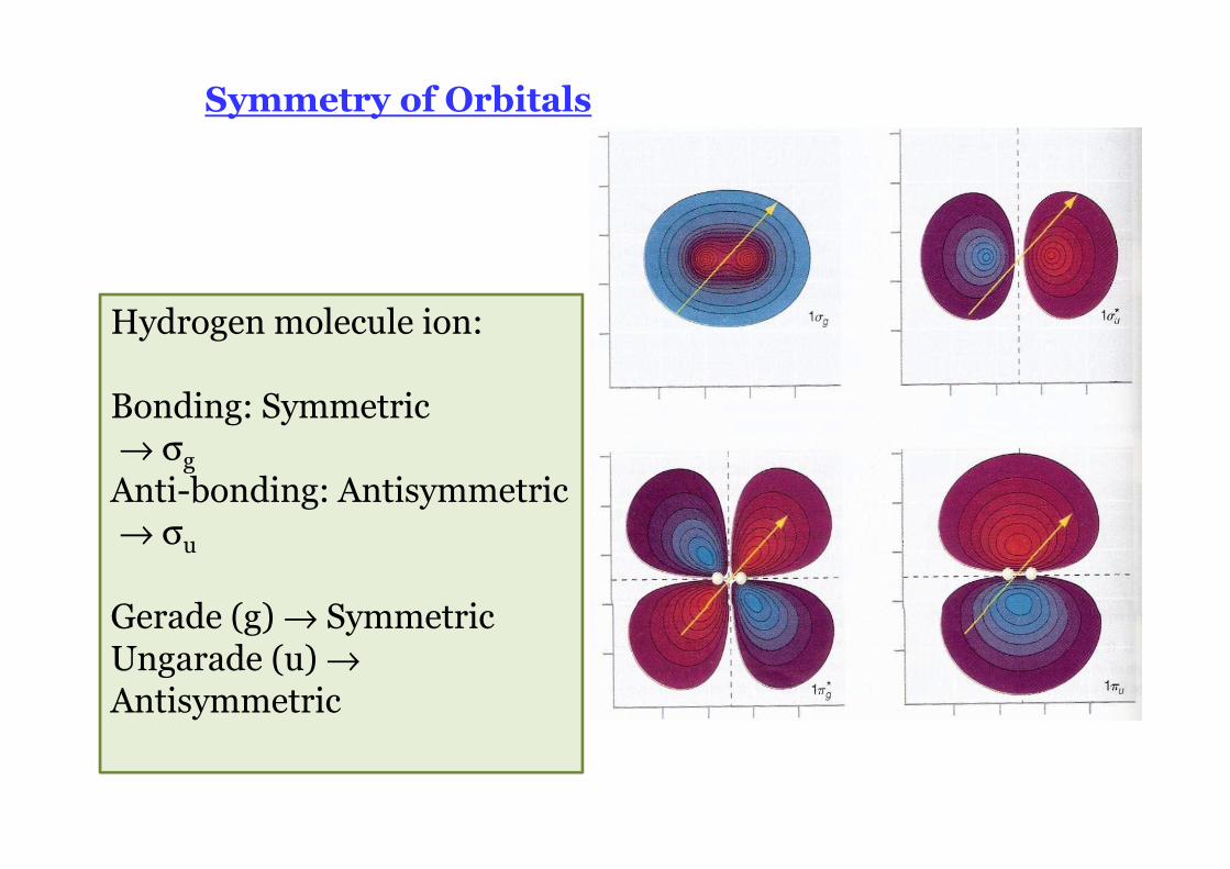
Symmetry of Orbitals
Hydrogen molecule ion:
Bonding: Symmetric→ σg
Anti-bonding: Antisymmetric→ σu
Gerade (g) → SymmetricUngarade (u) →Antisymmetric
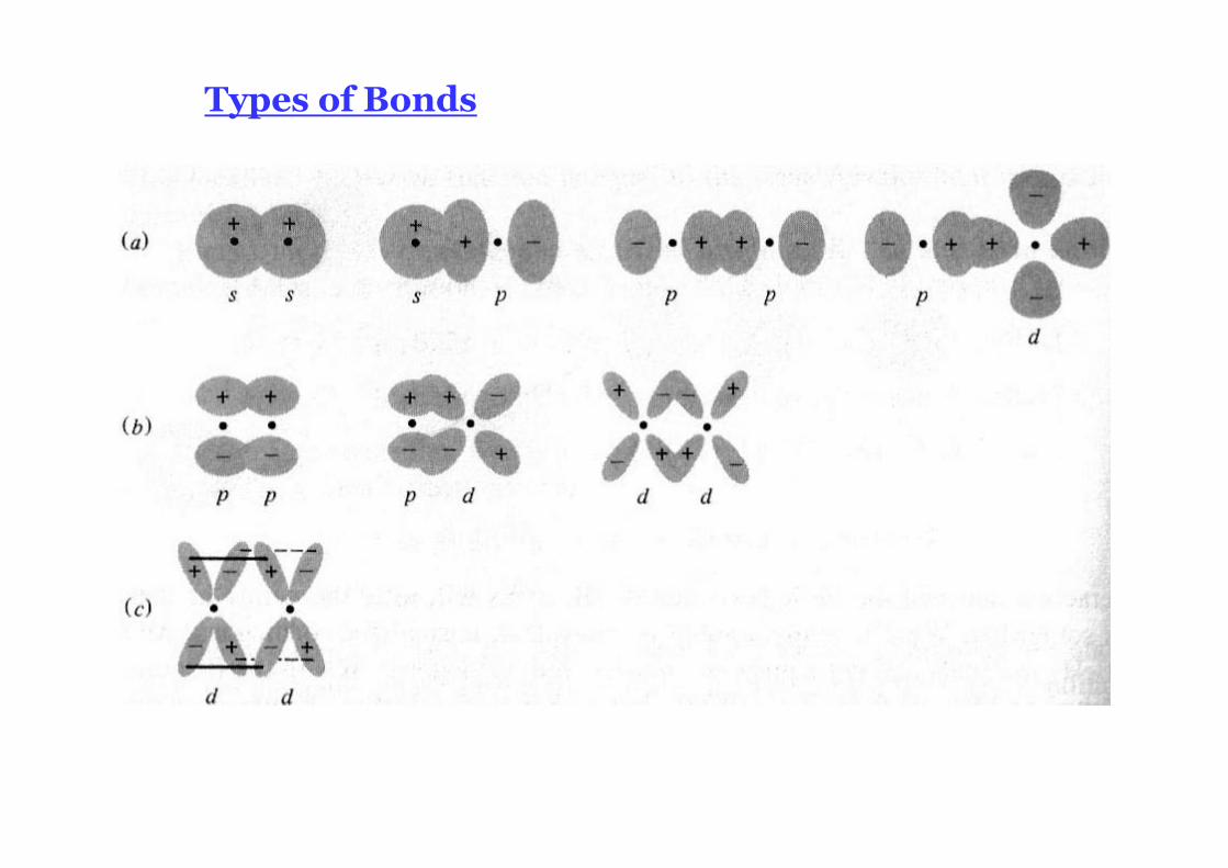
Types of Bonds
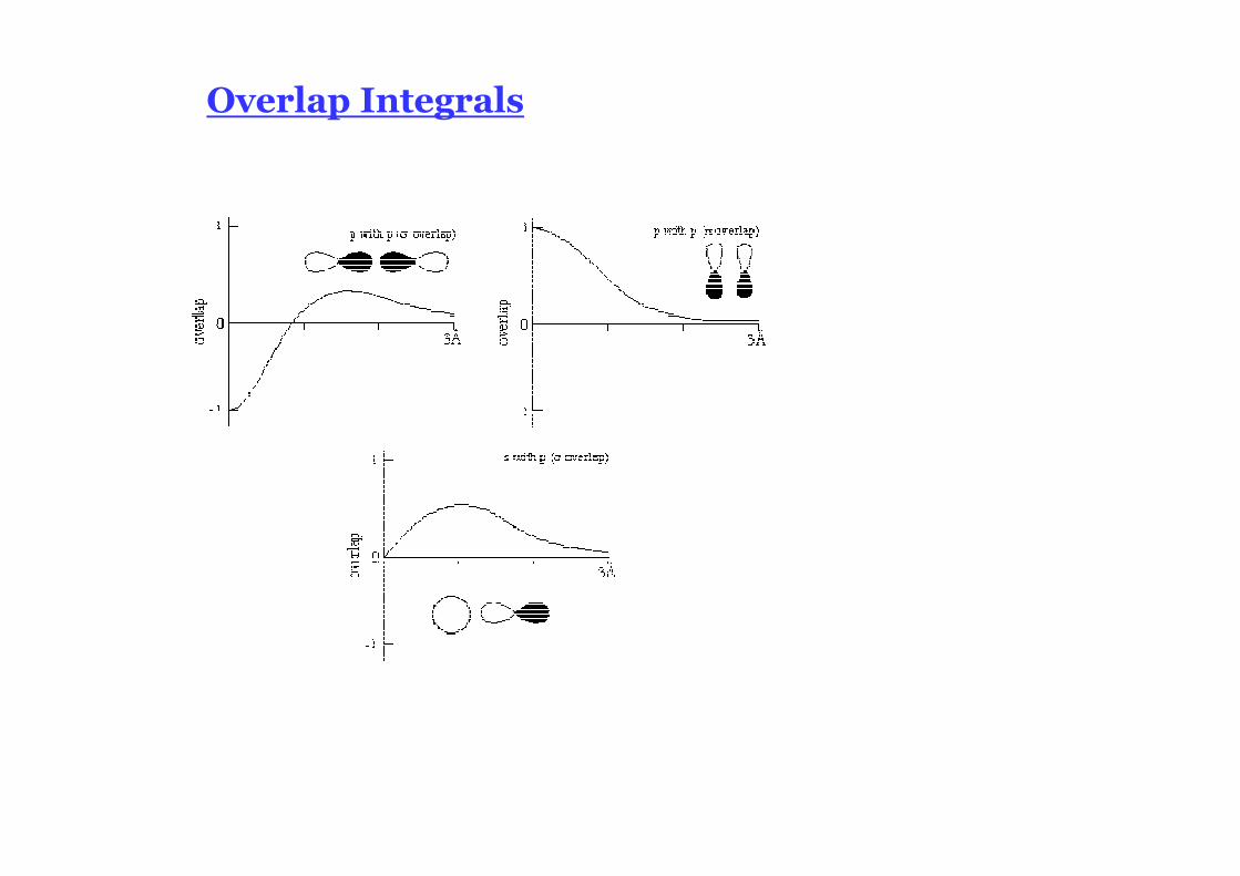
Overlap Integrals
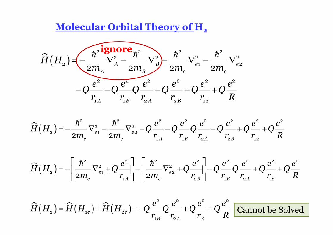
Molecular Orbital Theory of H2
� ( ) = − ∇ − ∇ − ∇ − ∇
− − − + +
� � � �2 2 2 2
2 2 2 22 1 2
2 2 2 2 2 2
1 1 2 2 12
2 2 2 2
A B e eA B e e
A B A B
H Hm m m m
e e e e e eQ Q Q Q Q Qr r r r r R
� ( )
� ( )
� ( ) � ( ) � ( )
= − ∇ − ∇ − − − + +
= − ∇ + − ∇ + − + +
= + − − + +
� �
� �
2 2 2 2 2 2 2 22 2
2 1 21 1 2 2 12
2 2 2 2 2 2 2 22 2
2 1 21 2 1 2 12
2 2 2 2
2 1 21 2 12
2 2
2 2
e ee e A B A B
e ee A e B B A
e eB A
e e e e e eH H Q Q Q Q Q Q
m m r r r r r R
e e e e e eH H Q Q Q Q Q Q
m r m r r r r R
e e e eH H H H H H Q Q Q Q
r r r R
ignore
Cannot be Solved
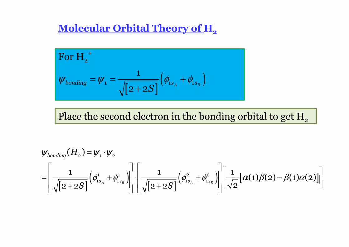
Molecular Orbital Theory of H2
For H2+
[ ]( )ψ ψ φ φ= = +
+1 1 1
1
2 2 A Bbonding s sS
Place the second electron in the bonding orbital to get H2
[ ]( )
[ ]( ) [ ]
ψ ψ ψ
φ φ φ φ α β β α
= ⋅
= + ⋅ + − + +
2 1 2
1 1 2 21 1 1 1
( )
1 1 1(1) (2) (1) (2)
22 2 2 2A B A B
bonding
s s s s
H
S S
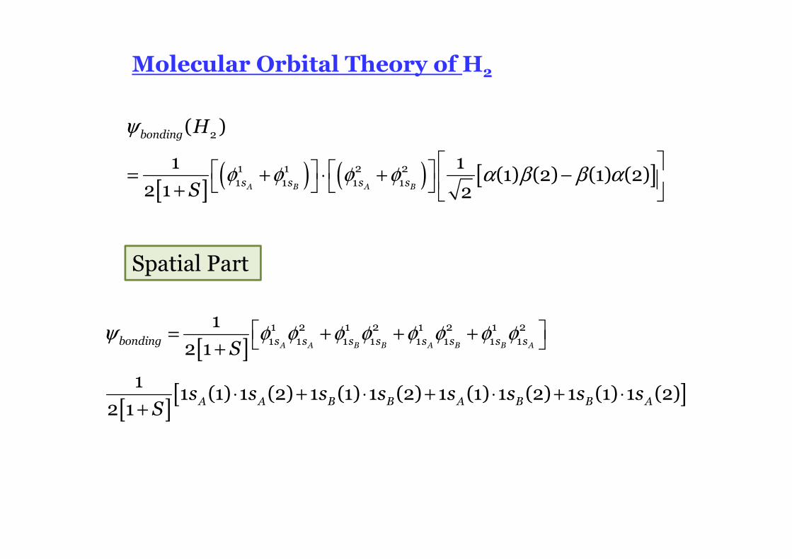
Molecular Orbital Theory of H2
[ ]( ) ( ) [ ]
ψ
φ φ φ φ α β β α = + ⋅ + − +
2
1 1 2 21 1 1 1
( )
1 1(1) (2) (1) (2)
2 1 2A B A B
bonding
s s s s
H
S
[ ]
[ ][ ]
ψ φ φ φ φ φ φ φ φ = + + + +
⋅ + ⋅ + ⋅ + ⋅+
1 2 1 2 1 2 1 21 1 1 1 1 1 1 1
12 1
11 (1) 1 (2) 1 (1) 1 (2) 1 (1) 1 (2) 1 (1) 1 (2)
2 1
A A B B A B B Abonding s s s s s s s s
A A B B A B B A
S
s s s s s s s sS
Spatial Part
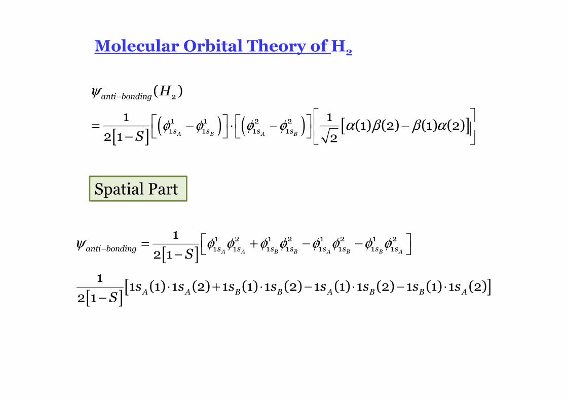
Molecular Orbital Theory of H2
[ ]( ) ( ) [ ]
ψ
φ φ φ φ α β β α
−
= − ⋅ − − −
2
1 1 2 21 1 1 1
( )
1 1(1) (2) (1) (2)
2 1 2A B A B
anti bonding
s s s s
H
S
[ ]
[ ][ ]
ψ φ φ φ φ φ φ φ φ− = + − − −
⋅ + ⋅ − ⋅ − ⋅−
1 2 1 2 1 2 1 21 1 1 1 1 1 1 1
12 1
11 (1) 1 (2) 1 (1) 1 (2) 1 (1) 1 (2) 1 (1) 1 (2)
2 1
A A B B A B B Aanti bonding s s s s s s s s
A A B B A B B A
S
s s s s s s s sS
Spatial Part
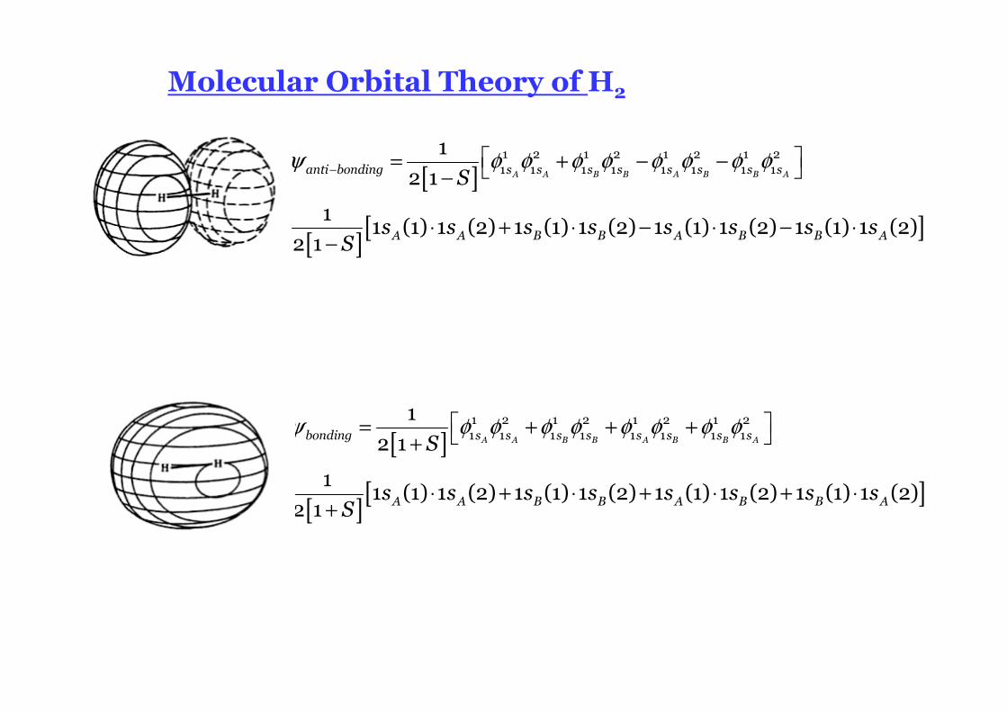
Molecular Orbital Theory of H2
[ ]
[ ][ ]
ψ φ φ φ φ φ φ φ φ = + + + +
⋅ + ⋅ + ⋅ + ⋅+
1 2 1 2 1 2 1 21 1 1 1 1 1 1 1
1
2 1
11 (1) 1 (2) 1 (1) 1 (2) 1 (1) 1 (2) 1 (1) 1 (2)
2 1
A A B B A B B Abonding s s s s s s s s
A A B B A B B A
S
s s s s s s s sS
[ ]
[ ][ ]
ψ φ φ φ φ φ φ φ φ− = + − − −
⋅ + ⋅ − ⋅ − ⋅−
1 2 1 2 1 2 1 21 1 1 1 1 1 1 1
1
2 1
11 (1) 1 (2) 1 (1) 1 (2) 1 (1) 1 (2) 1 (1) 1 (2)
2 1
A A B B A B B Aanti bonding s s s s s s s s
A A B B A B B A
S
s s s s s s s sS
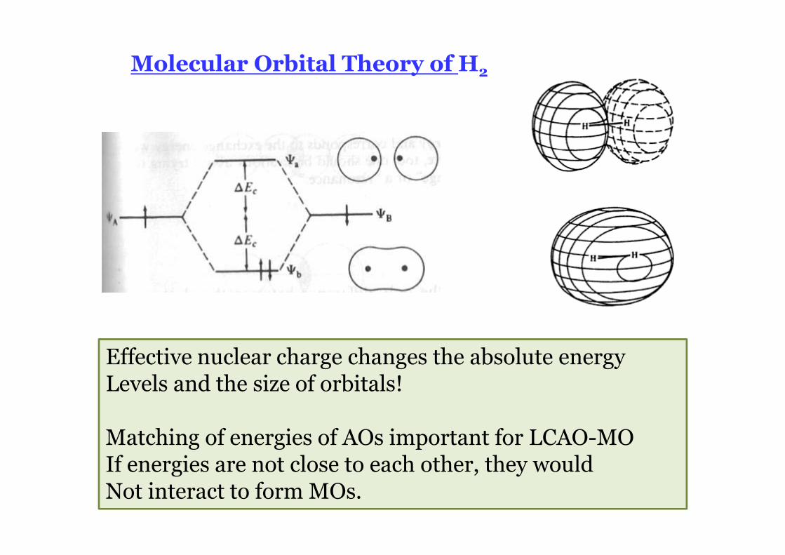
Molecular Orbital Theory of H2
Effective nuclear charge changes the absolute energyLevels and the size of orbitals!
Matching of energies of AOs important for LCAO-MOIf energies are not close to each other, they wouldNot interact to form MOs.
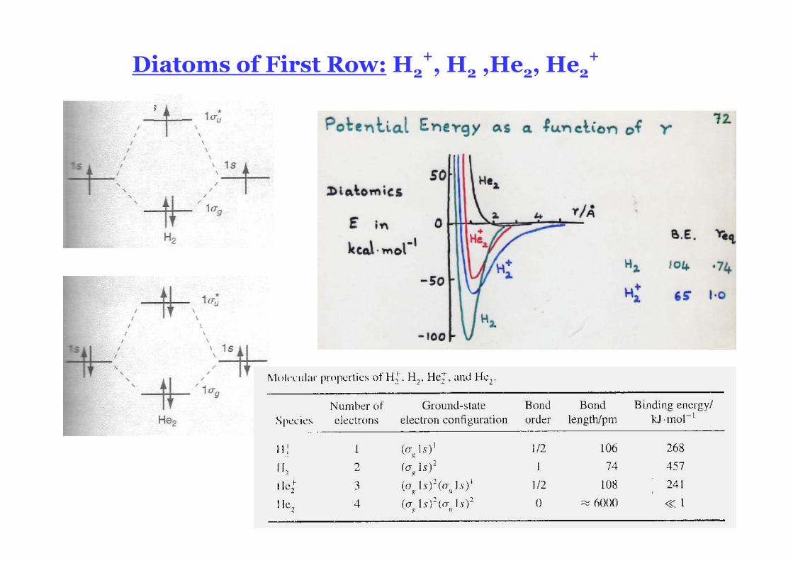
Diatoms of First Row: H2+, H2 ,He2, He2
+
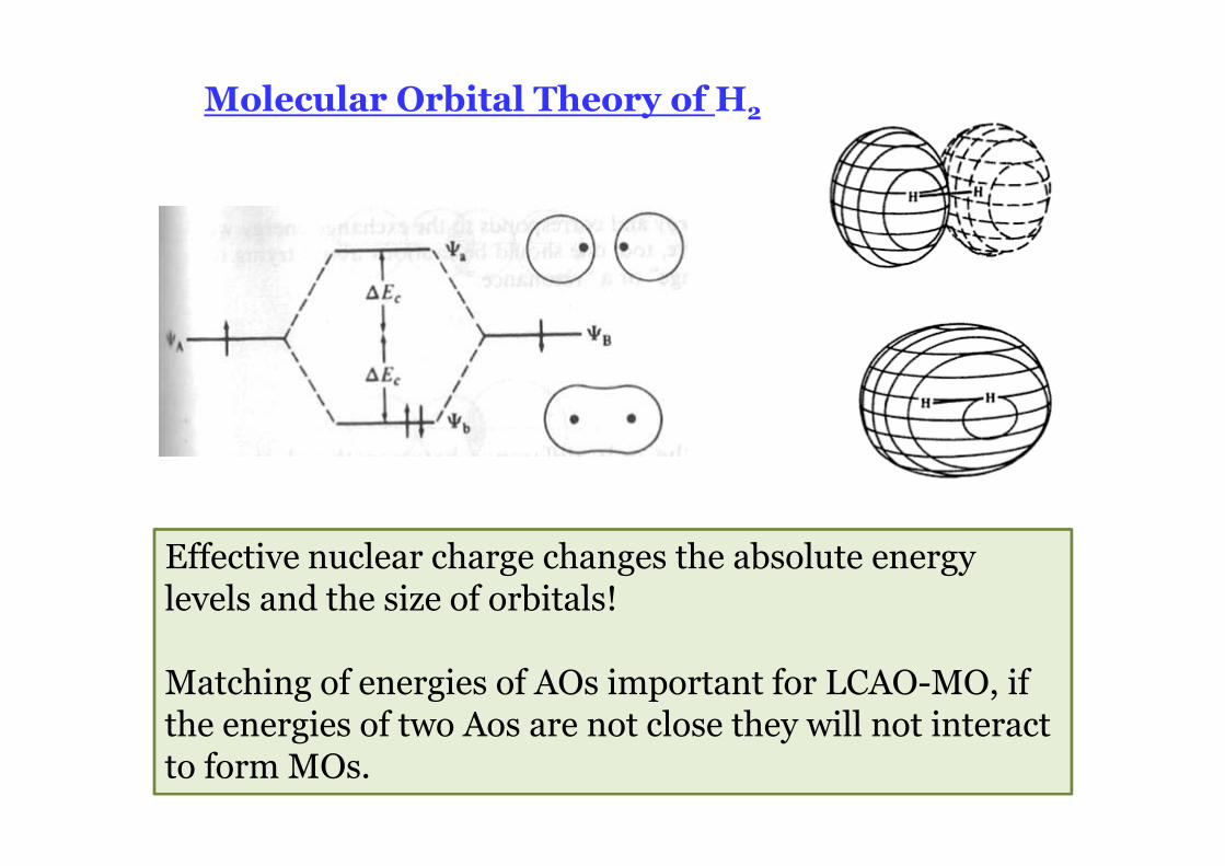
Molecular Orbital Theory of H2
Effective nuclear charge changes the absolute energylevels and the size of orbitals!
Matching of energies of AOs important for LCAO-MO, if the energies of two Aos are not close they will not interact to form MOs.
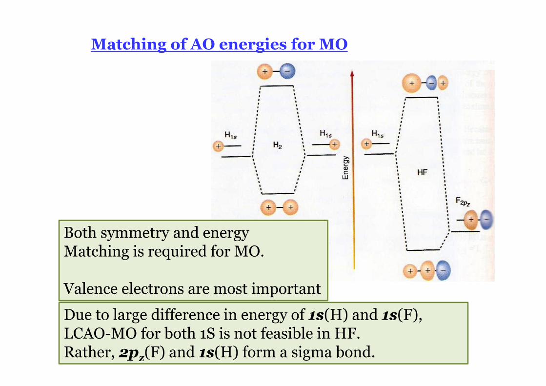
Matching of AO energies for MO
Due to large difference in energy of 1s(H) and 1s(F), LCAO-MO for both 1S is not feasible in HF. Rather, 2pz(F) and 1s(H) form a sigma bond.
Both symmetry and energyMatching is required for MO.
Valence electrons are most important
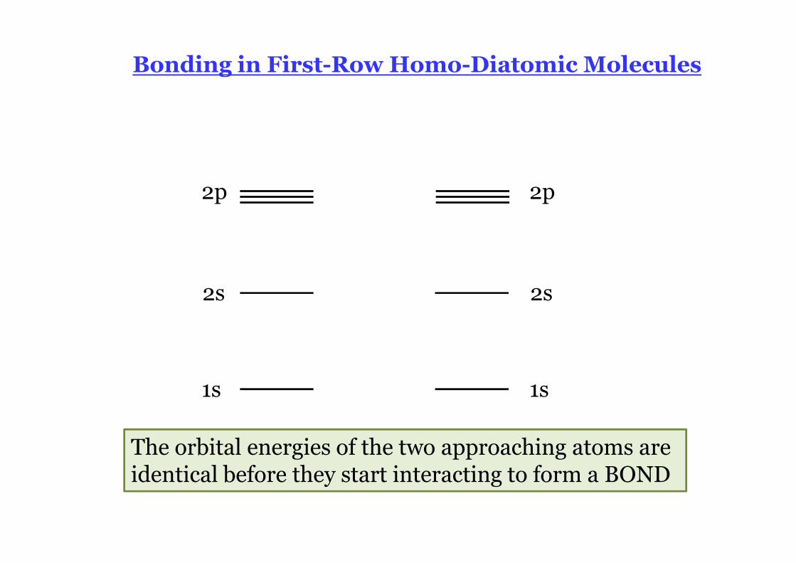
Bonding in First-Row Homo-Diatomic Molecules
1s
2s
2p
1s
2s
2p
The orbital energies of the two approaching atoms are identical before they start interacting to form a BOND
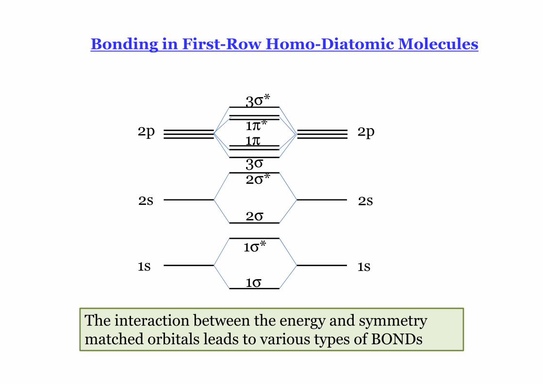
Bonding in First-Row Homo-Diatomic Molecules
1s
2s
2p
1s
2s
2p
1σ
1σ*
2σ
2σ*3σ
3σ*
1π1π*
The interaction between the energy and symmetry matched orbitals leads to various types of BONDs
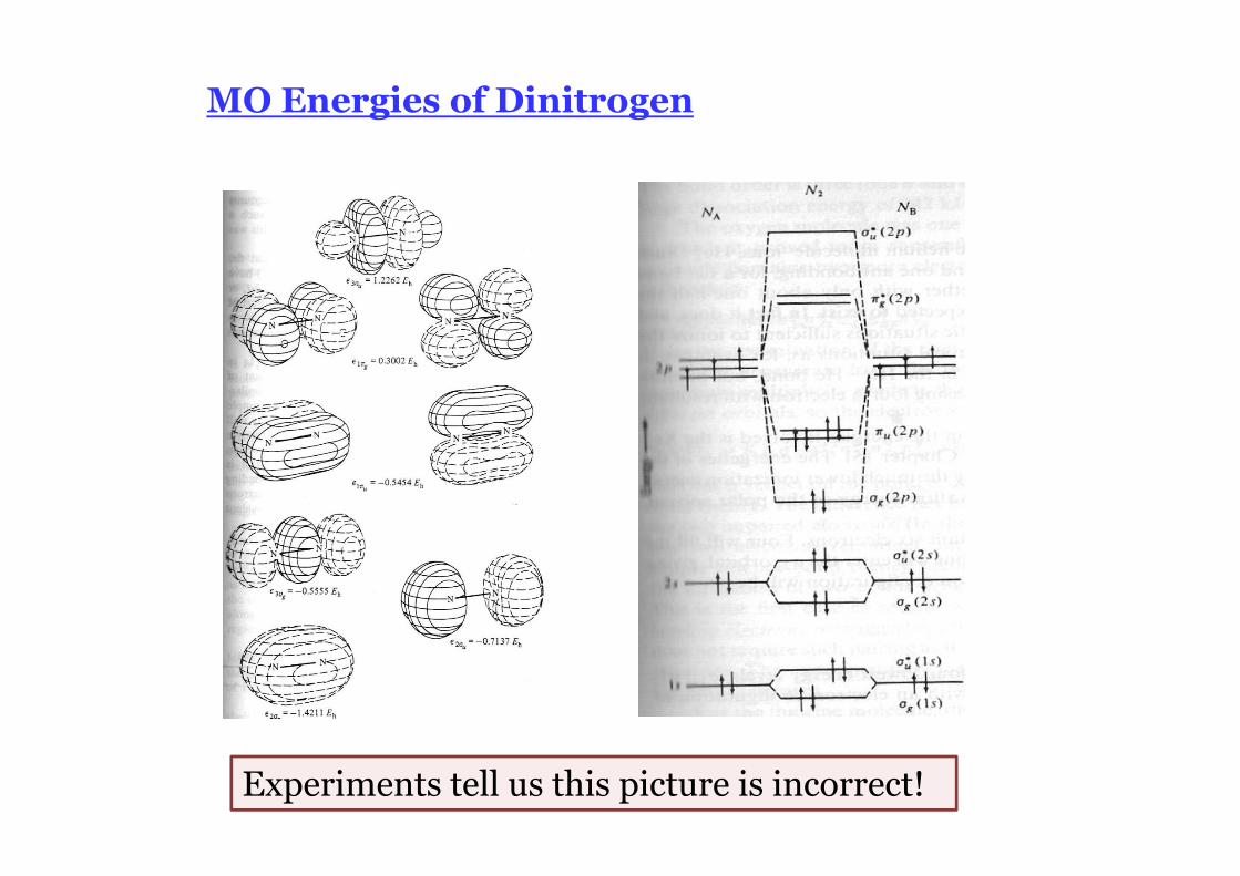
MO Energies of Dinitrogen
Experiments tell us this picture is incorrect!
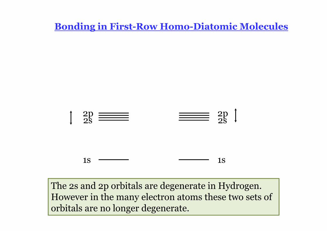
Bonding in First-Row Homo-Diatomic Molecules
1s
2s2p
1s
2s2p
The 2s and 2p orbitals are degenerate in Hydrogen. However in the many electron atoms these two sets of orbitals are no longer degenerate.
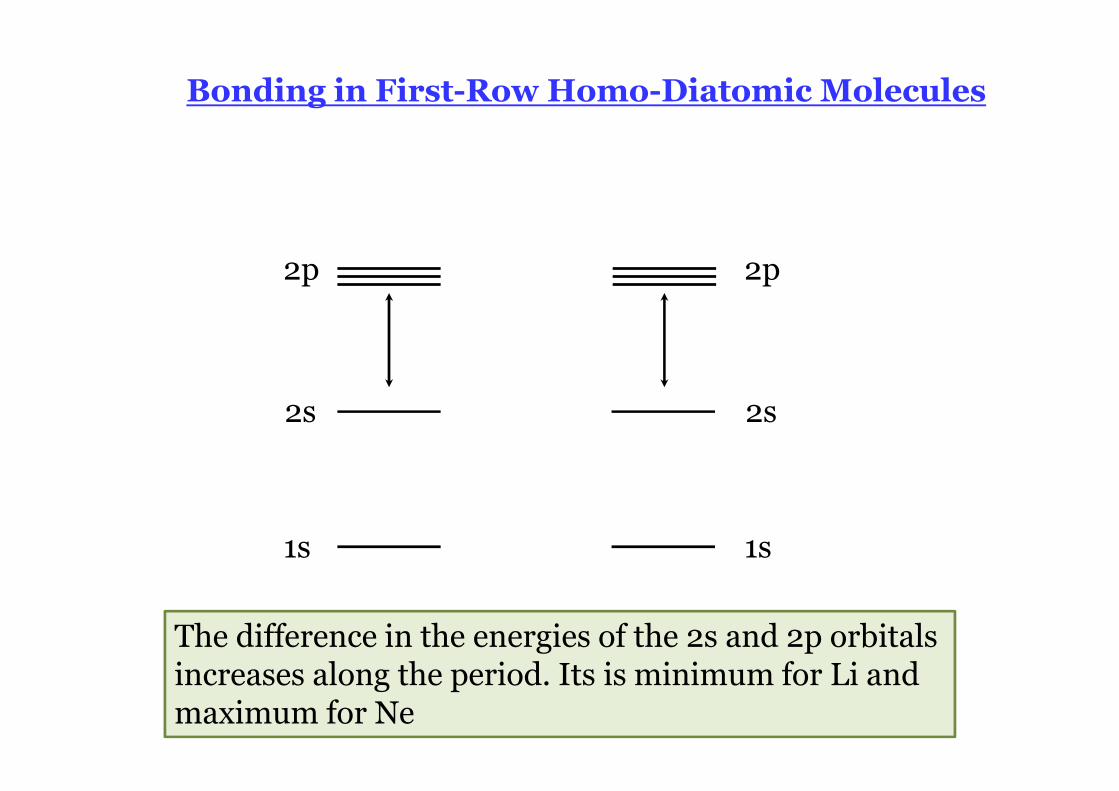
Bonding in First-Row Homo-Diatomic Molecules
1s
2s
2p
1s
2s
2p
The difference in the energies of the 2s and 2p orbitals increases along the period. Its is minimum for Li and maximum for Ne

MO Energies of Dinitrogen
Mixing of 2s and 2p orbital occur because of small energy gap between them2s and 2p electrons feels not so different nuclear charge.
Note how the MO of 2s→σ have p-type looks, while π-levels are clean
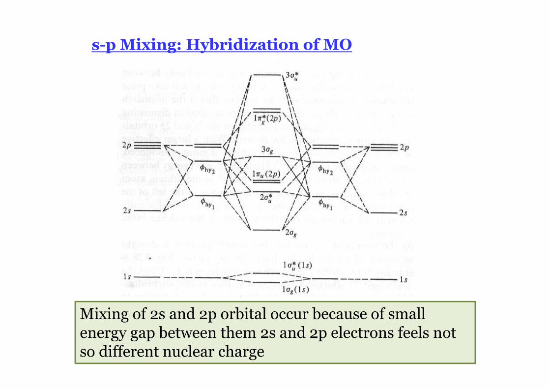
s-p Mixing: Hybridization of MO
Mixing of 2s and 2p orbital occur because of small energy gap between them 2s and 2p electrons feels not so different nuclear charge
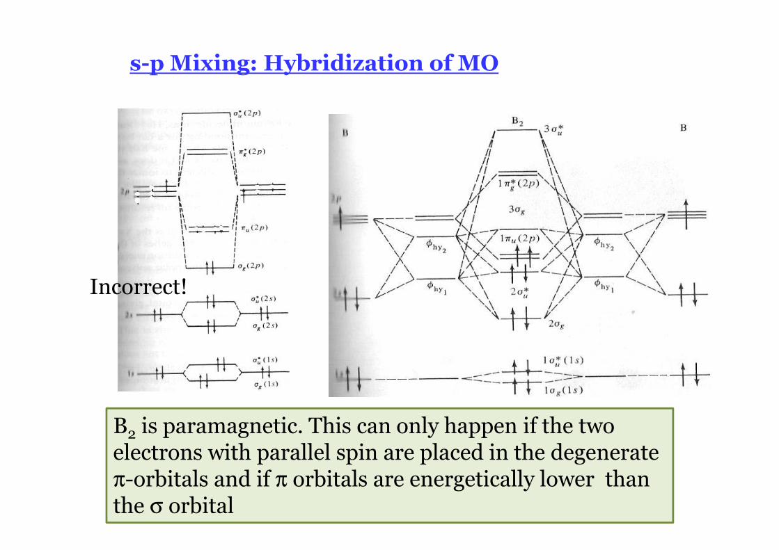
s-p Mixing: Hybridization of MO
B2 is paramagnetic. This can only happen if the two electrons with parallel spin are placed in the degenerate π-orbitals and if π orbitals are energetically lower than the σ orbital
Incorrect!
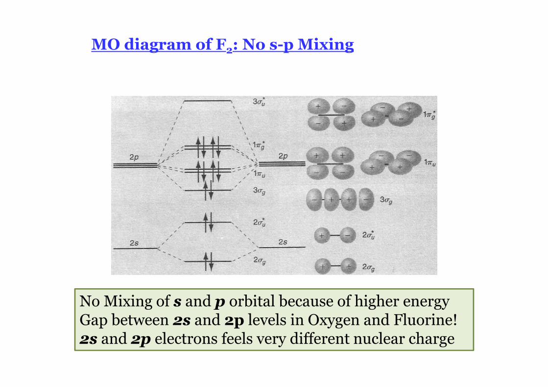
MO diagram of F2: No s-p Mixing
No Mixing of s and p orbital because of higher energyGap between 2s and 2p levels in Oxygen and Fluorine!2s and 2p electrons feels very different nuclear charge
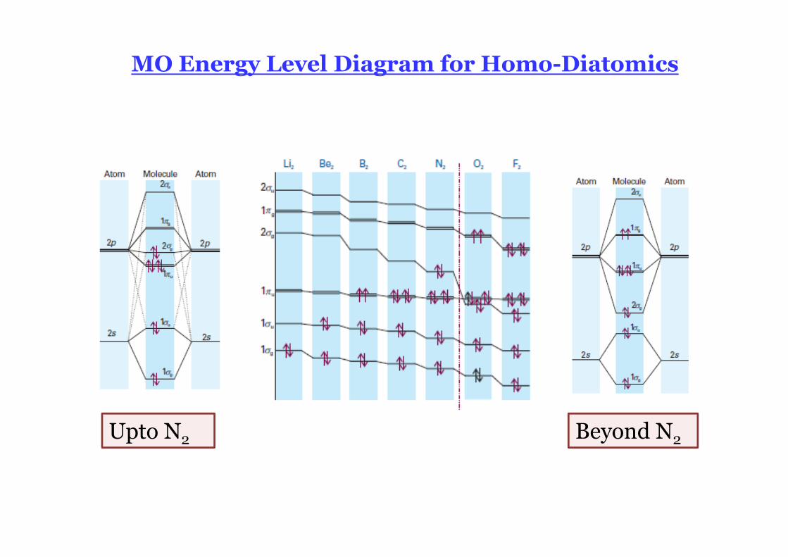
MO Energy Level Diagram for Homo-Diatomics
Upto N2 Beyond N2
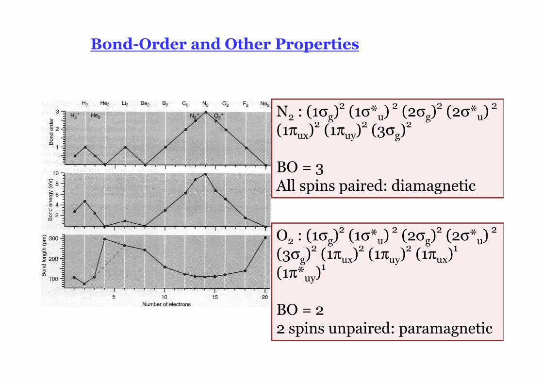
Bond-Order and Other Properties
N2 : (1σg)2 (1σ*u)
2 (2σg)2 (2σ*u)
2
(1πux)2 (1πuy)
2 (3σg)2
BO = 3 All spins paired: diamagnetic
O2 : (1σg)2 (1σ*u)
2 (2σg)2 (2σ*u)
2
(3σg)2 (1πux)
2 (1πuy)2 (1πux)
1
(1π*uy)1
BO = 2 2 spins unpaired: paramagnetic
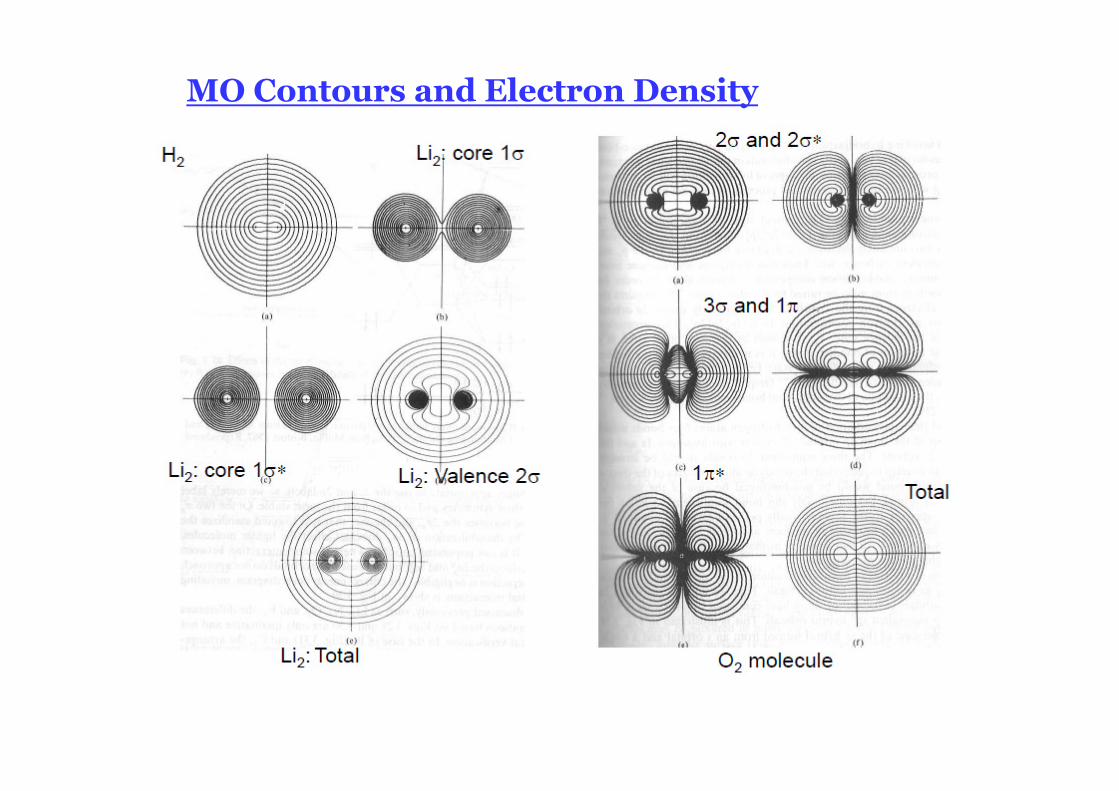
MO Contours and Electron Density
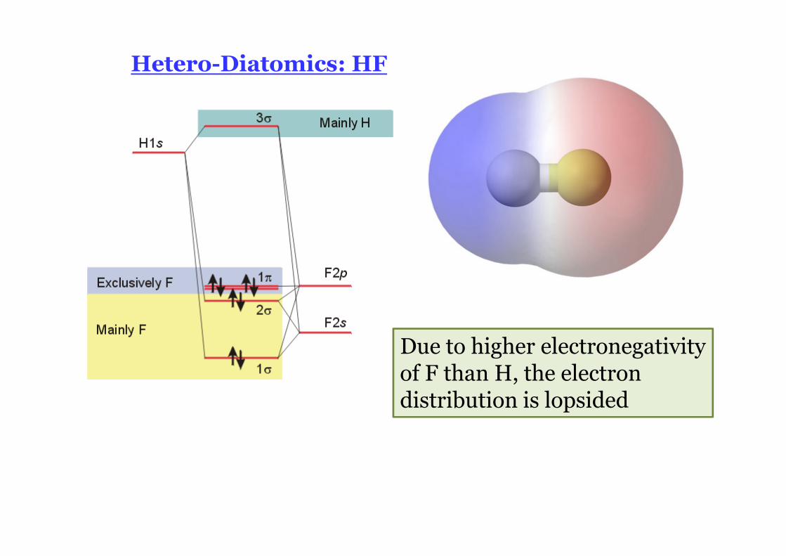
Hetero-Diatomics: HF
Due to higher electronegativityof F than H, the electron distribution is lopsided
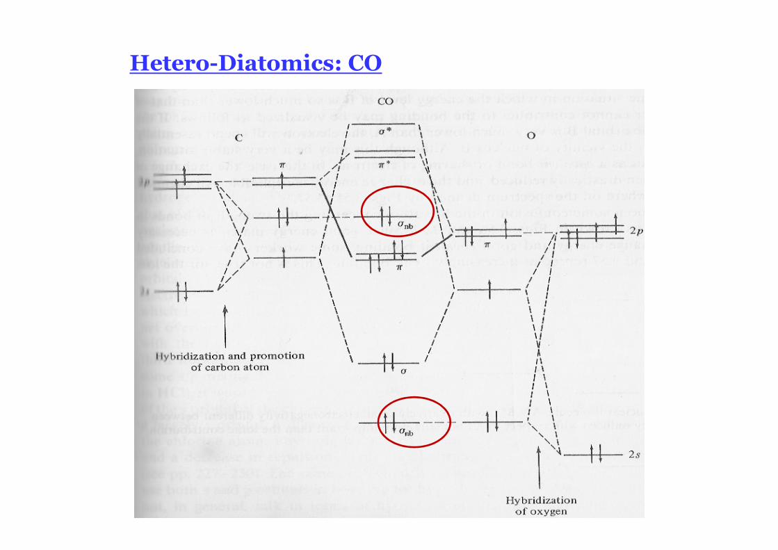
Hetero-Diatomics: CO
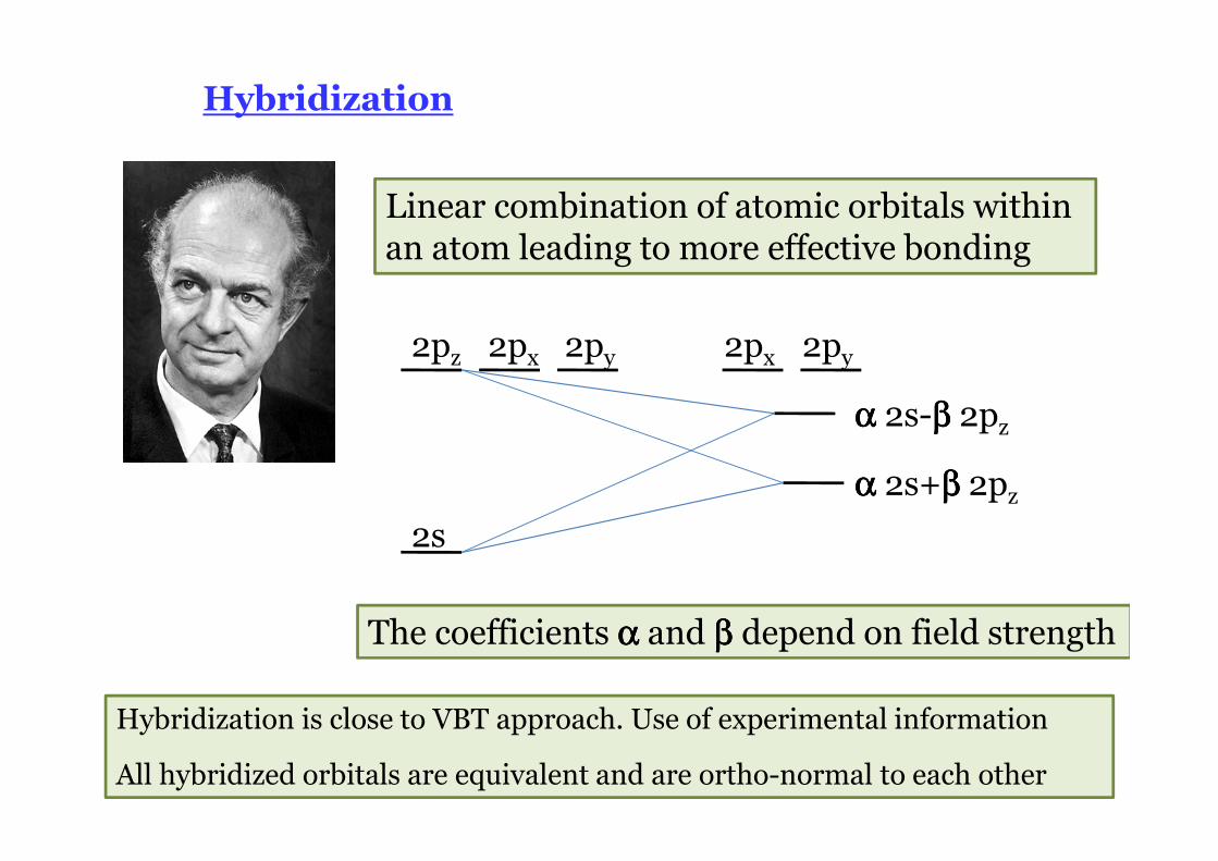
Hybridization
Linear combination of atomic orbitals within an atom leading to more effective bonding
2s
2pz 2px 2py 2px 2py
αααα 2s-ββββ 2pz
αααα 2s+ββββ 2pz
The coefficients αααα and ββββ depend on field strength
Hybridization is close to VBT approach. Use of experimental information
All hybridized orbitals are equivalent and are ortho-normal to each other
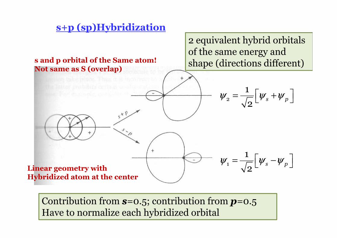
Contribution from s=0.5; contribution from p=0.5Have to normalize each hybridized orbital
= − 1
1
2s pψ ψ ψ
= + 2
1
2s pψ ψ ψ
2 equivalent hybrid orbitalsof the same energy andshape (directions different)
Linear geometry with Hybridized atom at the center
s and p orbital of the Same atom! Not same as S (overlap)
s+p (sp)Hybridization
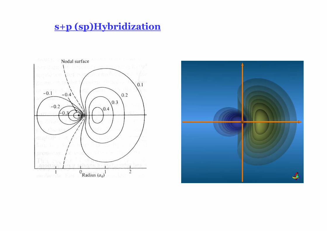
s+p (sp)Hybridization
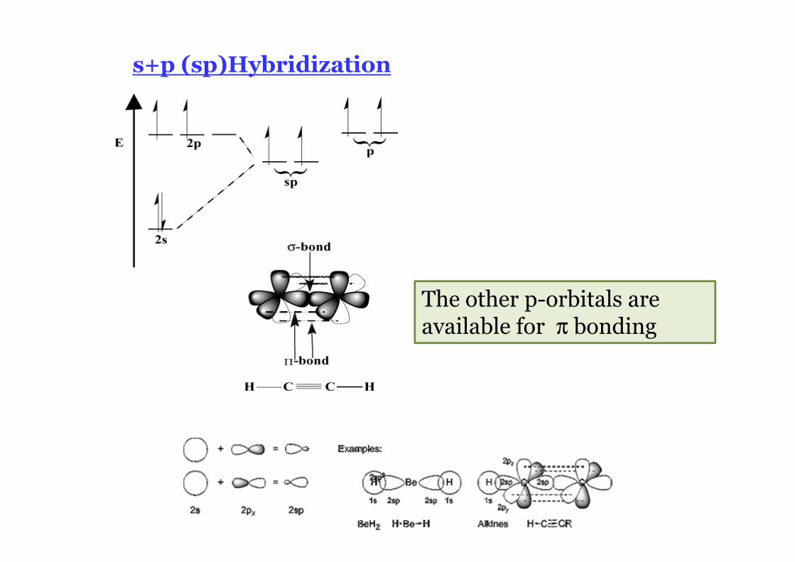
The other p-orbitals are available for π bonding
s+p (sp)Hybridization
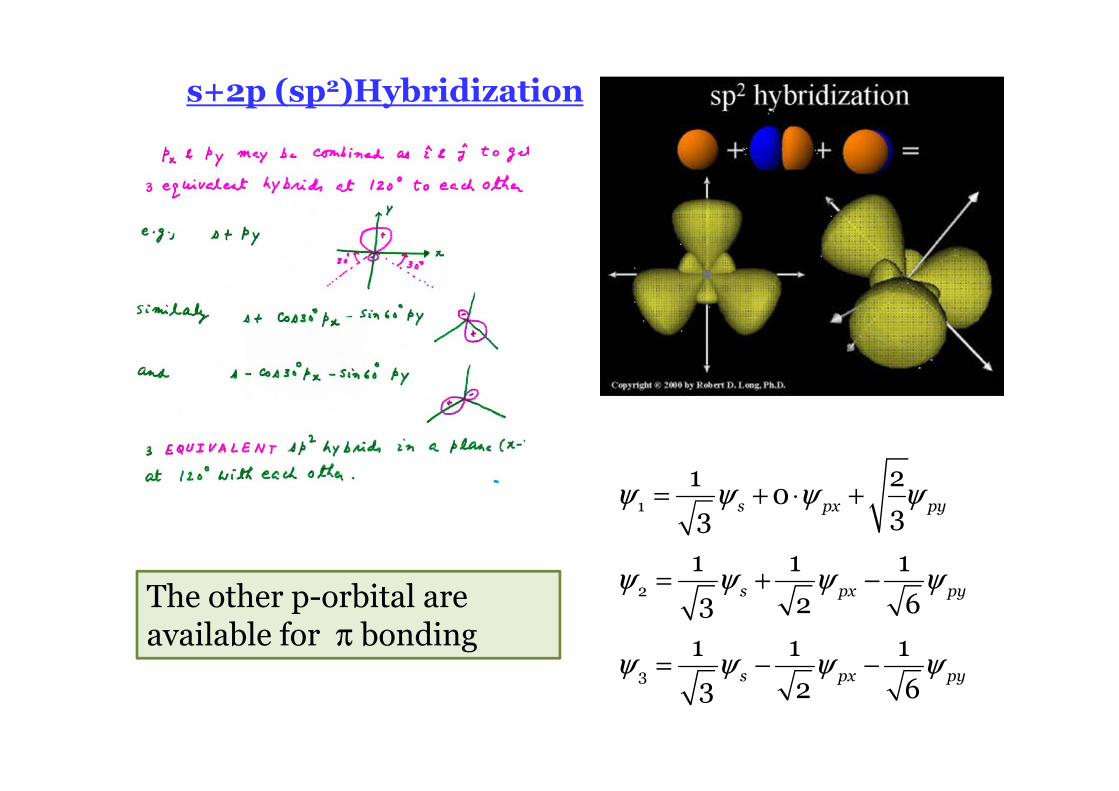
1
2
3
1 20
33
1 1 1
3 2 6
1 1 1
3 2 6
s px py
s px py
s px py
ψ ψ ψ ψ
ψ ψ ψ ψ
ψ ψ ψ ψ
= + ⋅ +
= + −
= − −
The other p-orbital are available for π bonding
s+2p (sp2)Hybridization
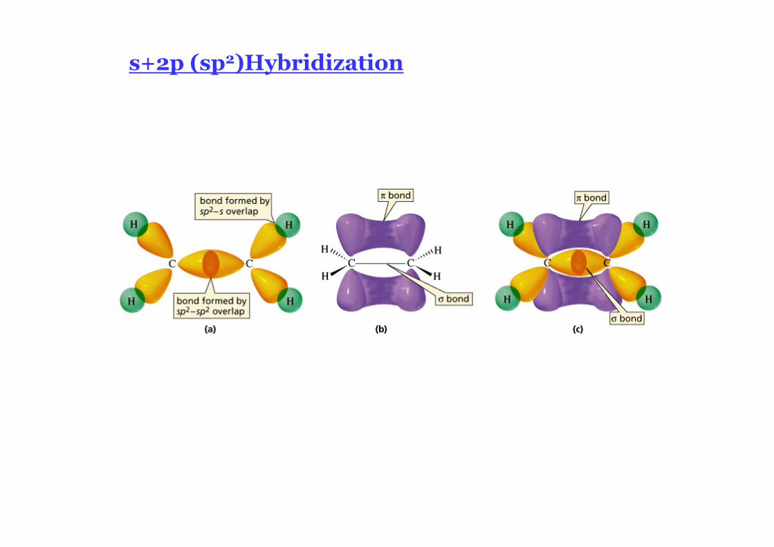
s+2p (sp2)Hybridization
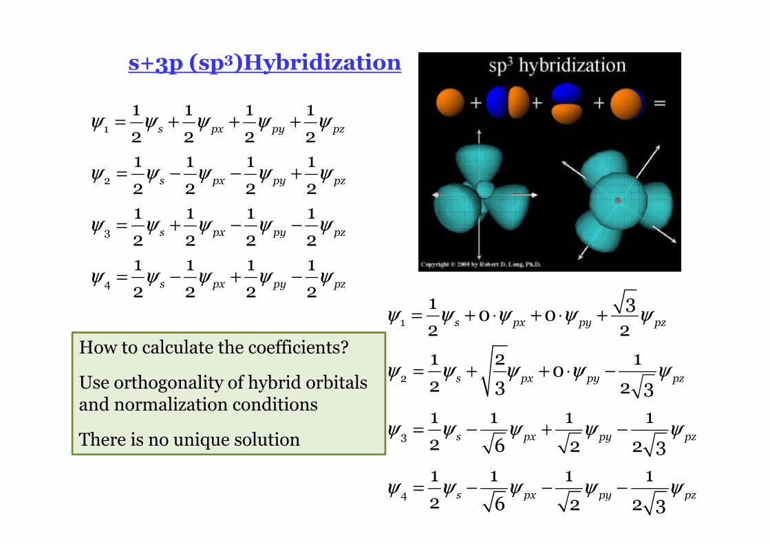
1
2
3
4
1 1 1 1
2 2 2 21 1 1 1
2 2 2 21 1 1 1
2 2 2 21 1 1 12 2 2 2
s px py pz
s px py pz
s px py pz
s px py pz
ψ ψ ψ ψ ψ
ψ ψ ψ ψ ψ
ψ ψ ψ ψ ψ
ψ ψ ψ ψ ψ
= + + +
= − − +
= + − −
= − + −
How to calculate the coefficients?
Use orthogonality of hybrid orbitalsand normalization conditions
There is no unique solution
1
2
3
4
1 30 0
2 2
1 2 10
2 3 2 3
1 1 1 12 6 2 2 3
1 1 1 1
2 6 2 2 3
s px py pz
s px py pz
s px py pz
s px py pz
ψ ψ ψ ψ ψ
ψ ψ ψ ψ ψ
ψ ψ ψ ψ ψ
ψ ψ ψ ψ ψ
= + ⋅ + ⋅ +
= + + ⋅ −
= − + −
= − − −
s+3p (sp3)Hybridization
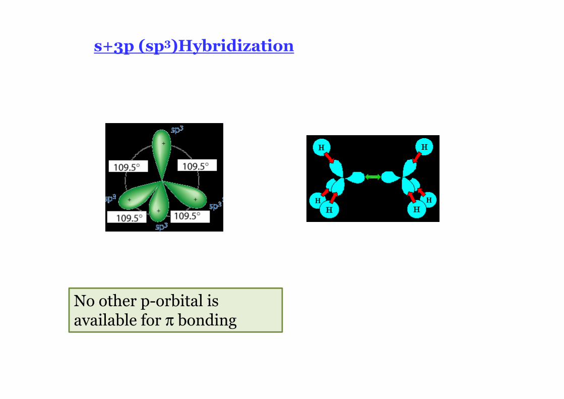
s+3p (sp3)Hybridization
No other p-orbital is available for π bonding
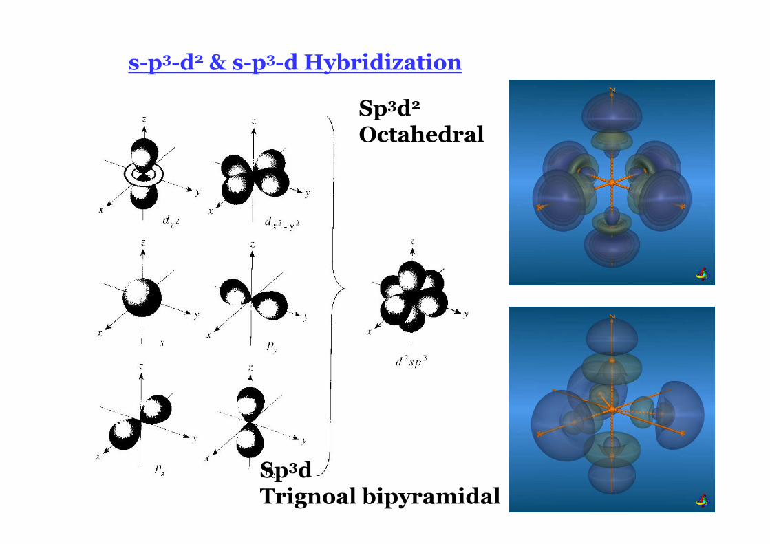
s-p3-d2 & s-p3-d Hybridization
Sp3d2
Octahedral
Sp3dTrignoal bipyramidal
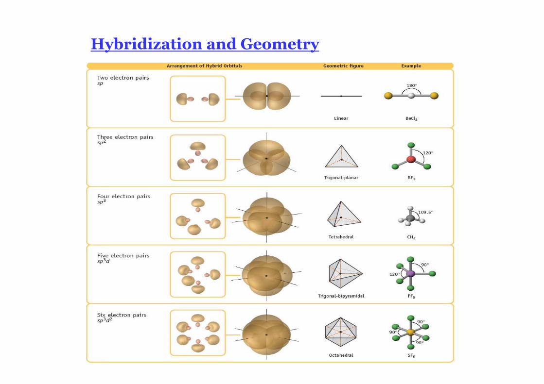
Hybridization and Geometry
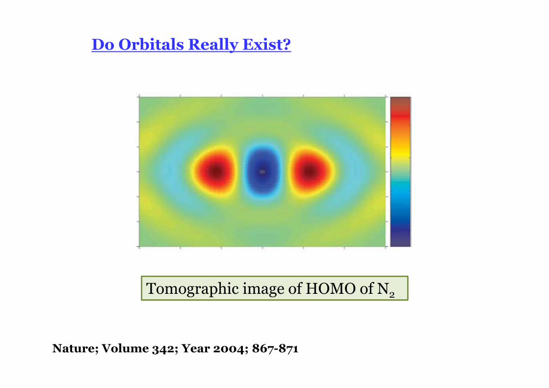
Do Orbitals Really Exist?
Tomographic image of HOMO of N2
Nature; Volume 342; Year 2004; 867-871

Collaboration between Chemists and Engineers
The tensile strength of spider silk is greater than the same weight of steel and has much greater elasticity