GNU Radio Tutorials

Labs 1 – 5

Balint SeeberEttus Research

Version 1.0 (18th April 2014)

Comments & suggetions welcome:balint@ettus.com@spenchdotnet

Lab 1

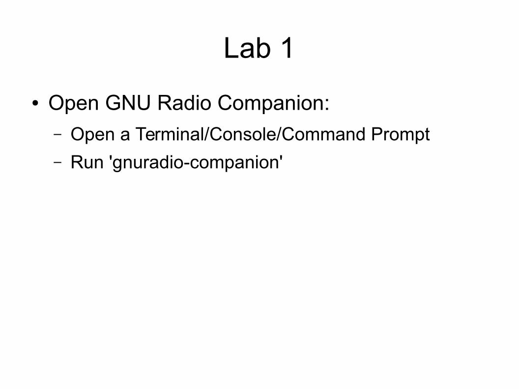
● Open GNU Radio Companion:– Open a Terminal/Console/Command Prompt

– Run 'gnuradio-companion'

Lab 1

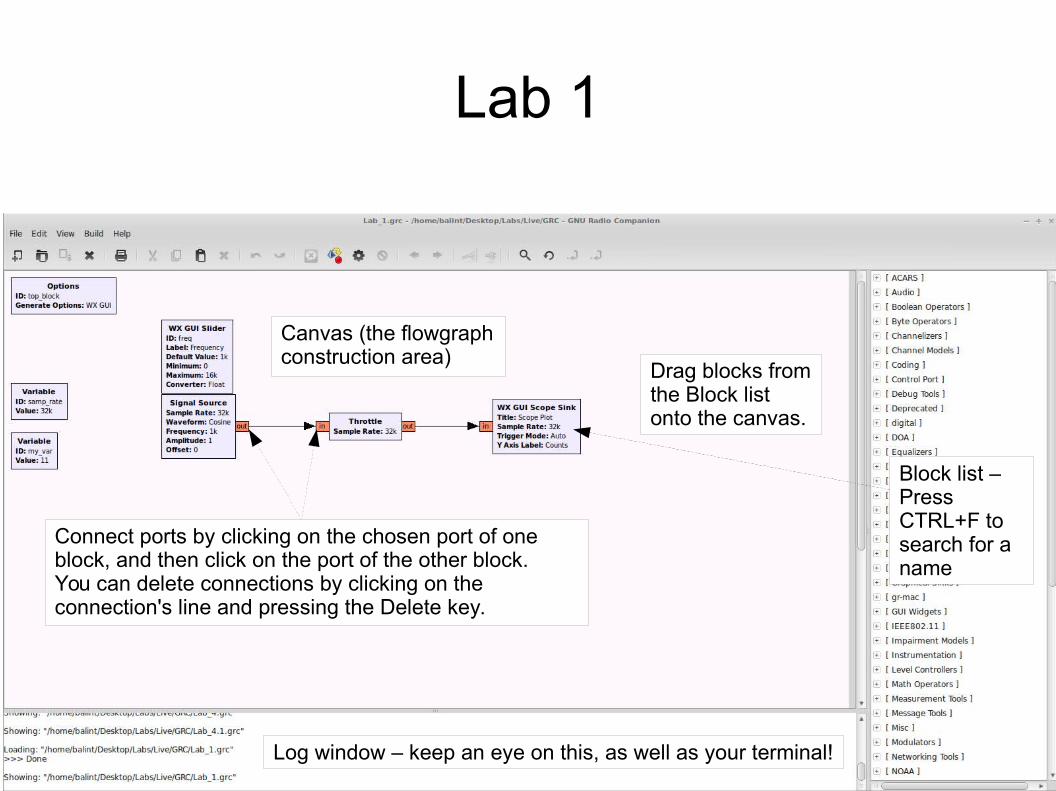
Log window – keep an eye on this, as well as your terminal!

Block list – Press CTRL+F to search for a name

Canvas (the flowgraph construction area)

Drag blocks from the Block list onto the canvas.

Connect ports by clicking on the chosen port of one block, and then click on the port of the other block.You can delete connections by clicking on the connection's line and pressing the Delete key.

Lab 1

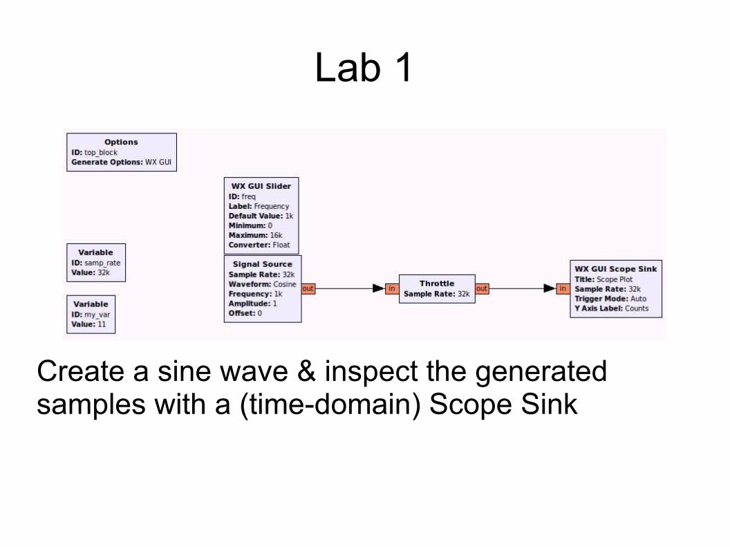
Create a sine wave & inspect the generated samples with a (time-domain) Scope Sink

Lab 1

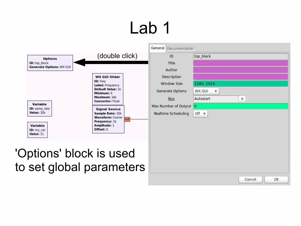
'Options' block is used to set global parameters

(double click)

Lab 1

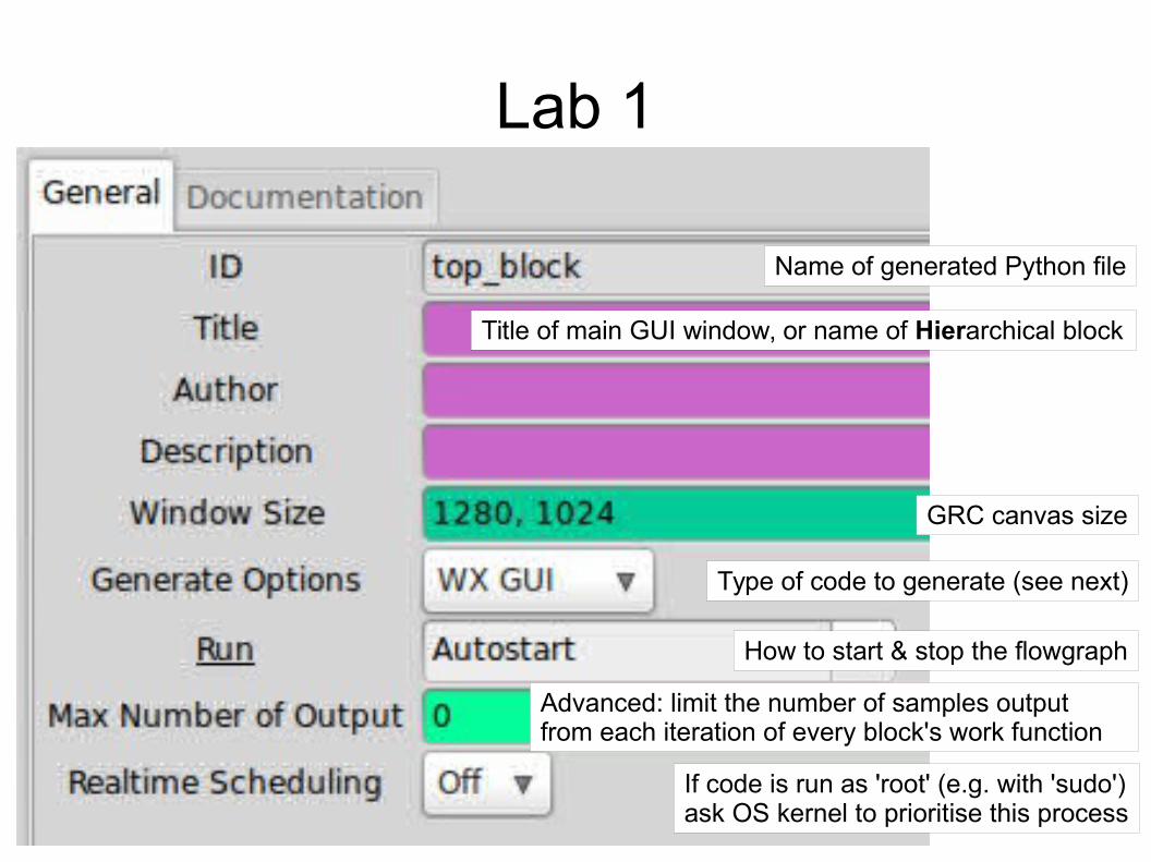
Name of generated Python file

Title of main GUI window, or name of Hierarchical block

GRC canvas size

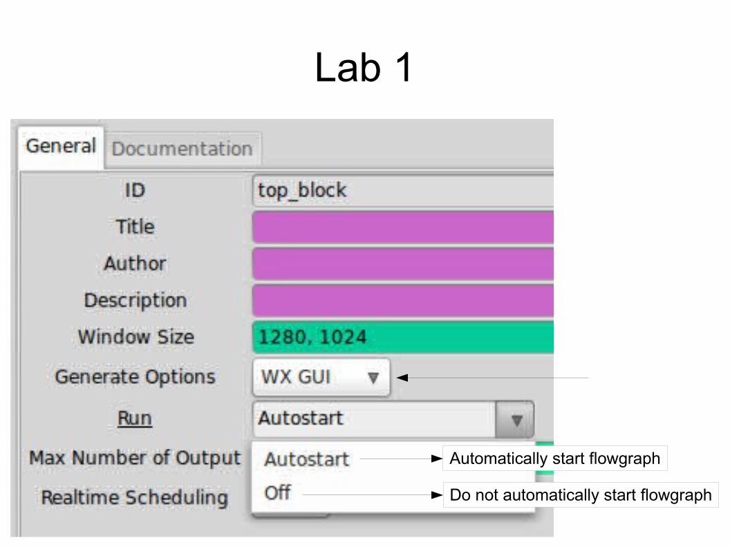
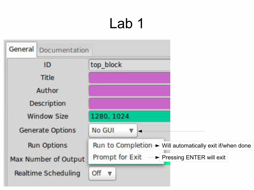
Type of code to generate (see next)

How to start & stop the flowgraph

If code is run as 'root' (e.g. with 'sudo')ask OS kernel to prioritise this process

Advanced: limit the number of samples output from each iteration of every block's work function

Lab 1

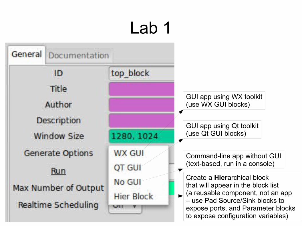
GUI app using WX toolkit(use WX GUI blocks)

GUI app using Qt toolkit(use Qt GUI blocks)

Command-line app without GUI(text-based, run in a console)

Create a Hierarchical block that will appear in the block list(a reusable component, not an app – use Pad Source/Sink blocks to expose ports, and Parameter blocks to expose configuration variables)

Lab 1

Automatically start flowgraph

Do not automatically start flowgraph

Lab 1

Will automatically exit if/when done

Pressing ENTER will exit

Lab 1

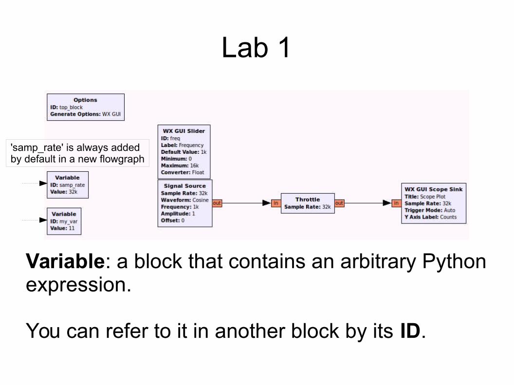
Variable: a block that contains an arbitrary Python expression.

You can refer to it in another block by its ID.

'samp_rate' is always added by default in a new flowgraph

Lab 1

(double click)

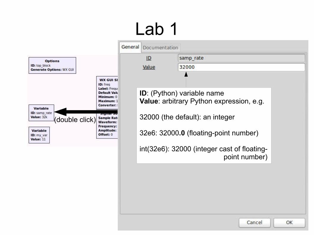
ID: (Python) variable nameValue: arbitrary Python expression, e.g.

32000 (the default): an integer

32e6: 32000.0 (floating-point number)

int(32e6): 32000 (integer cast of floating-point number)

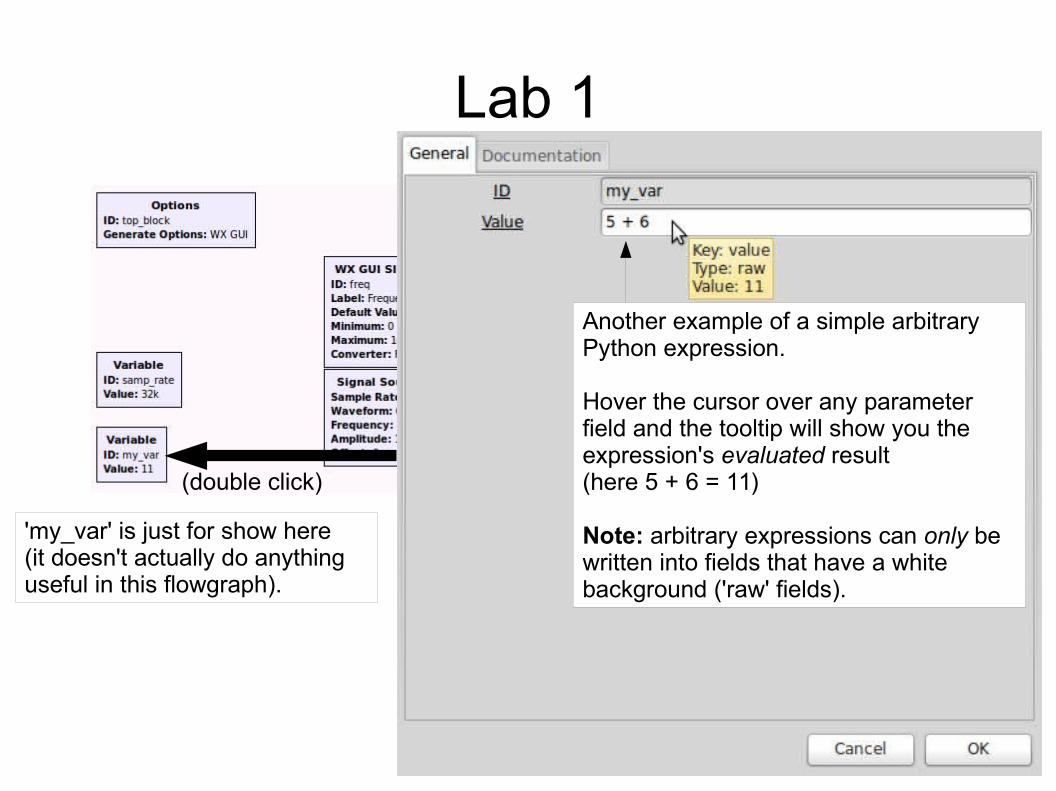
Lab 1

(double click)

Another example of a simple arbitrary Python expression.

Hover the cursor over any parameter field and the tooltip will show you the expression's evaluated result (here 5 + 6 = 11)

Note: arbitrary expressions can only be written into fields that have a white background ('raw' fields).

'my_var' is just for show here(it doesn't actually do anythinguseful in this flowgraph).

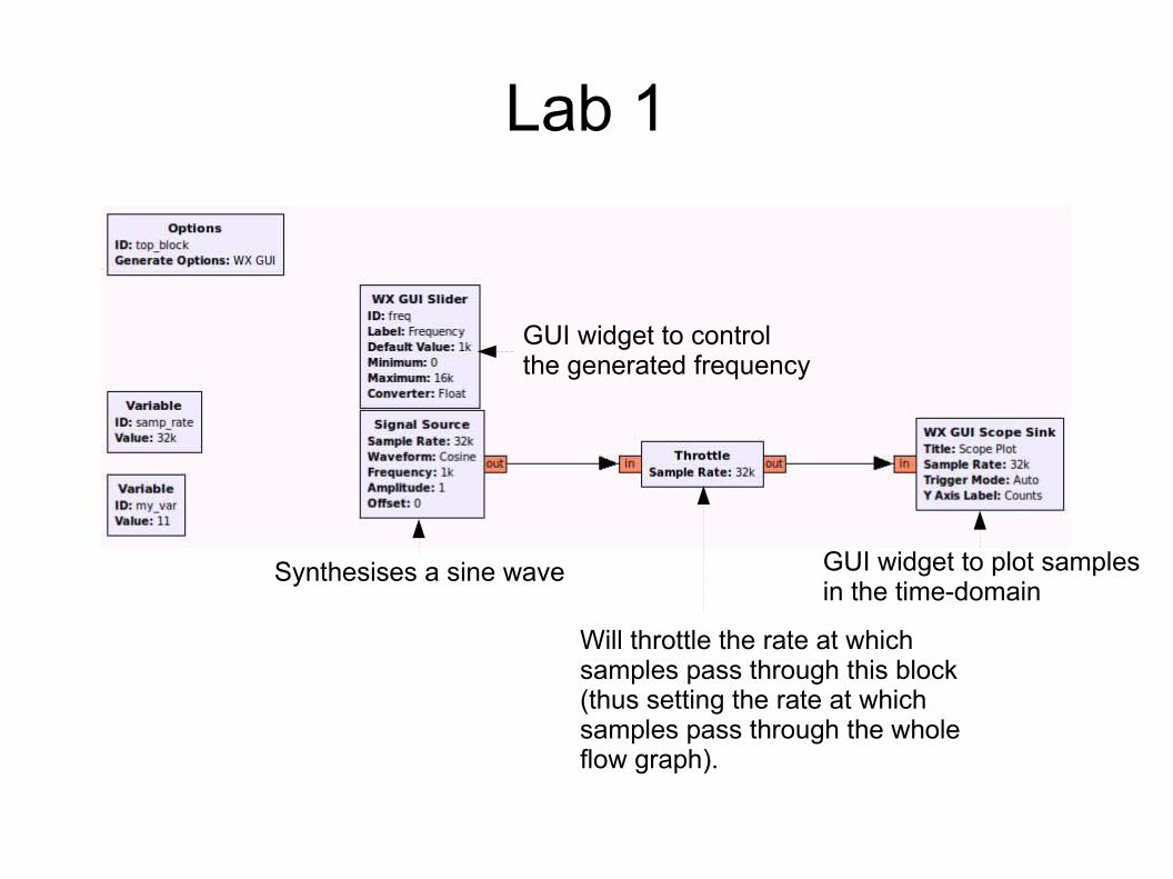
Lab 1

GUI widget to control the generated frequency

GUI widget to plot samples in the time-domain

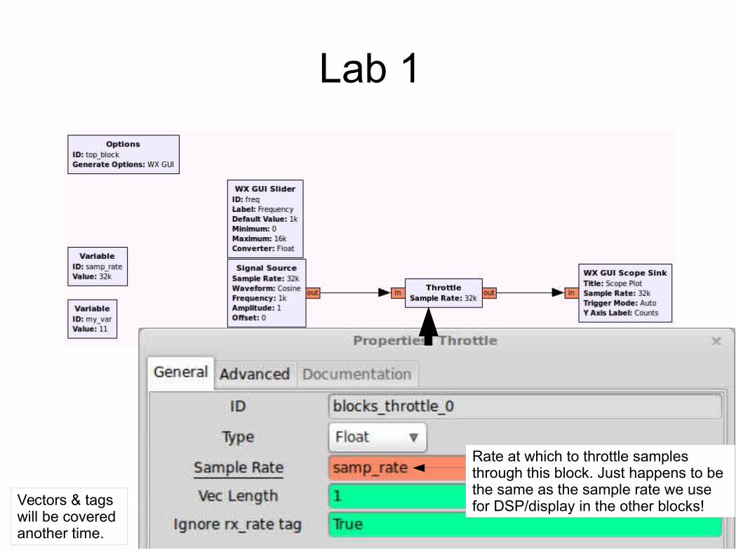
Will throttle the rate at which samples pass through this block(thus setting the rate at which samples pass through the whole flow graph).

Synthesises a sine wave

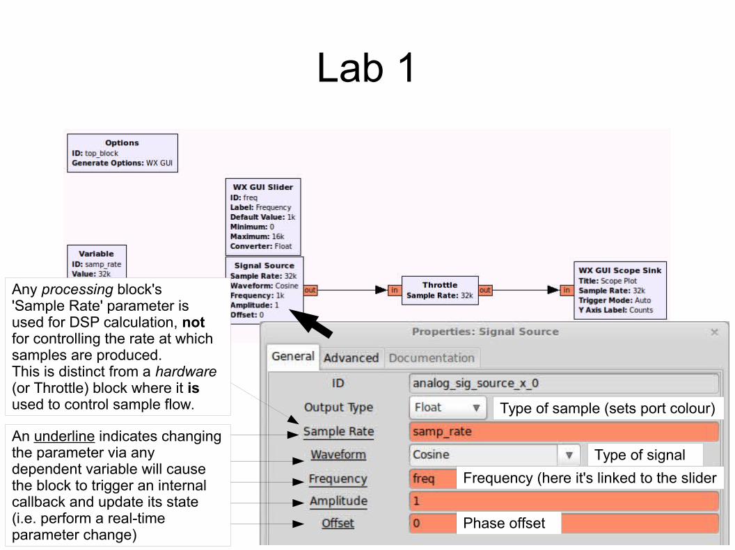
Lab 1

Type of sample (sets port colour)

Any processing block's 'Sample Rate' parameter is used for DSP calculation, not for controlling the rate at which samples are produced.This is distinct from a hardware (or Throttle) block where it is used to control sample flow.

Type of signal

Frequency (here it's linked to the slider

Phase offset

An underline indicates changing the parameter via any dependent variable will cause the block to trigger an internal callback and update its state (i.e. perform a real-time parameter change)

Sample Rate (DSP)

● If calculating a sine wave where a given frequency in Hertz is desired, you actually need to know the sample rate too. This is because the mathematical representation requires both values to calculate the individual sample amplitude at any specific point in time.

● The actual sample rate value used can be anything. It just so happens you'll usually use the same value as in the rest of your flowgraph so that everything will be consistent (operate in the same sample rate domain).

Sample Rate (DSP)

● Think of it as being used to calculate the discrete step size from one sample to the next within a DSP operation (e.g. the time step when calculating the amplitude of the next sample in the sine wave generator)

Sample Rate (Hardware)

● Distinct from mathematical (DSP) calculation, sample rate also refers to the rate at which samples pass through the flowgraph.

● If there is no rate control, hardware clock or throttling mechanism, the samples will be generated, pass through the flowgraph and be consumed as fast as possible (i.e. the flowgraph will be CPU bound).

● This is desirable if you want to perform some fixed DSP on stored data as quickly as possible (e.g. read from a file, resample and write it back).

Sample Rate (Hardware)

● Only a block that represents some underlying hardware with its own clock (e.g. USRP, sound card), or the Throttle Block, will use 'Sample Rate' to set that hardware clock, and therefore have the effect of applying rate control to the samples in the flowgraph.

● A Throttle Block will simply apply host-based timing (against the 'wall clock') to control the rate of the samples it produces (i.e. samples that it makes available on its outputs to downstream blocks).

Sample Rate (Hardware)

● A hardware Sink block will consume samples at a fixed rate (relative to the wall clock)

● The Throttle Block, or a hardware Sink block, will apply 'back pressure' to the upstream blocks (the rate of work of the upstream blocks will be limited by the throttling effect of this rate-controlling block)

● A hardware Source block will produce samples at a fixed rate (relative to the wall clock)

Sample Rate (Hardware)

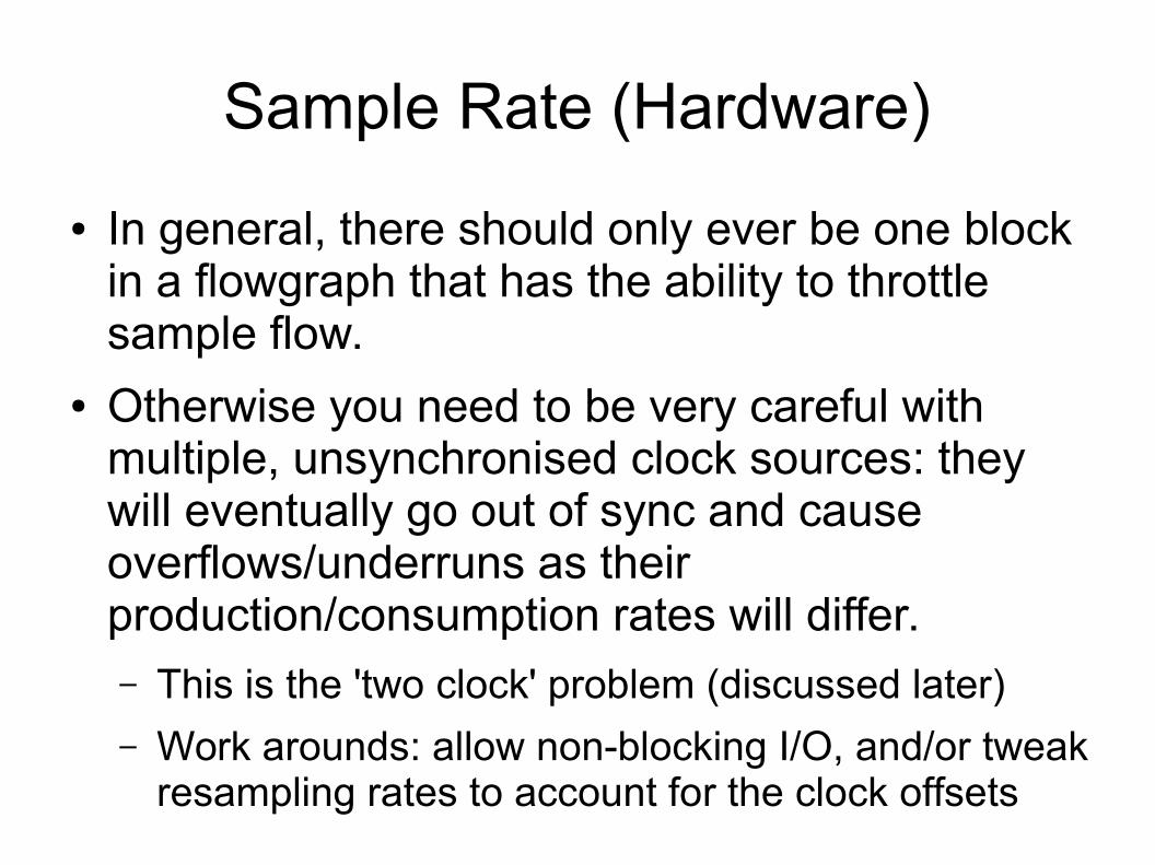
● In general, there should only ever be one block in a flowgraph that has the ability to throttle sample flow.

● Otherwise you need to be very careful with multiple, unsynchronised clock sources: they will eventually go out of sync and cause overflows/underruns as their production/consumption rates will differ.– This is the 'two clock' problem (discussed later)

– Work arounds: allow non-blocking I/O, and/or tweak resampling rates to account for the clock offsets

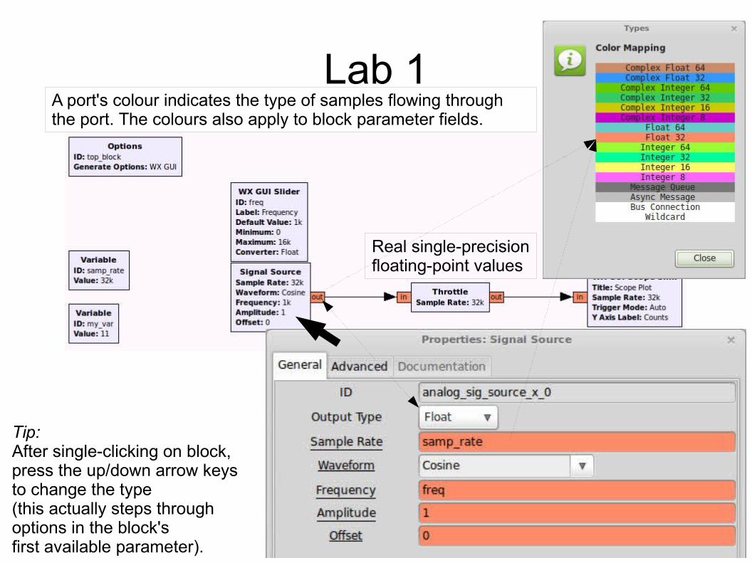
Lab 1A port's colour indicates the type of samples flowing through the port. The colours also apply to block parameter fields.

Tip:After single-clicking on block, press the up/down arrow keys to change the type(this actually steps through options in the block's first available parameter).

Real single-precision floating-point values

Lab 1

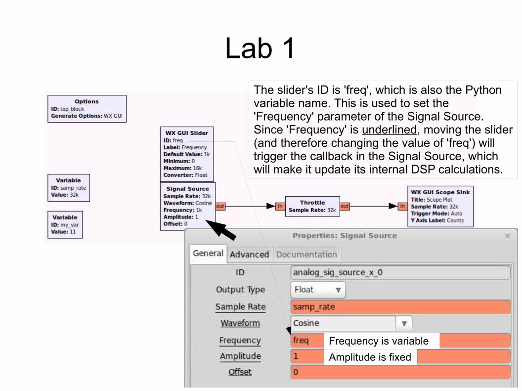
Amplitude is fixed

Frequency is variable

The slider's ID is 'freq', which is also the Pythonvariable name. This is used to set the 'Frequency' parameter of the Signal Source.Since 'Frequency' is underlined, moving the slider(and therefore changing the value of 'freq') will trigger the callback in the Signal Source, which will make it update its internal DSP calculations.

Lab 1

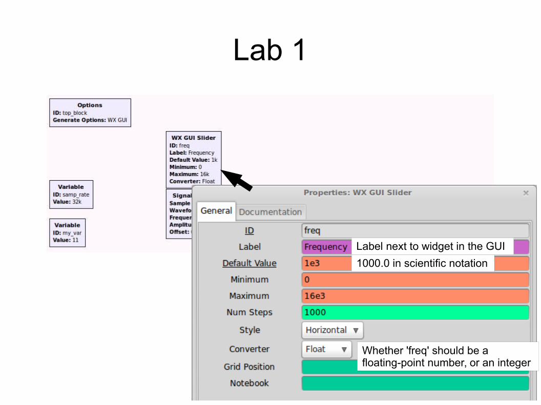
Whether 'freq' should be a floating-point number, or an integer

1000.0 in scientific notation

Label next to widget in the GUI

Lab 1

Rate at which to throttle samples through this block. Just happens to be the same as the sample rate we use for DSP/display in the other blocks!Vectors & tags

will be covered another time.

Lab 1

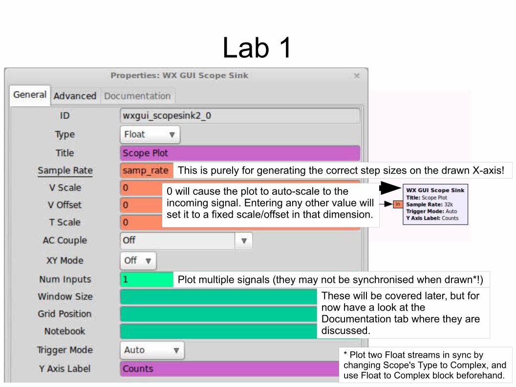
These will be covered later, but for now have a look at the Documentation tab where they are discussed.

Plot multiple signals (they may not be synchronised when drawn*!)

This is purely for generating the correct step sizes on the drawn X-axis!

* Plot two Float streams in sync by changing Scope's Type to Complex, and use Float to Complex block beforehand.

0 will cause the plot to auto-scale to the incoming signal. Entering any other value will set it to a fixed scale/offset in that dimension.

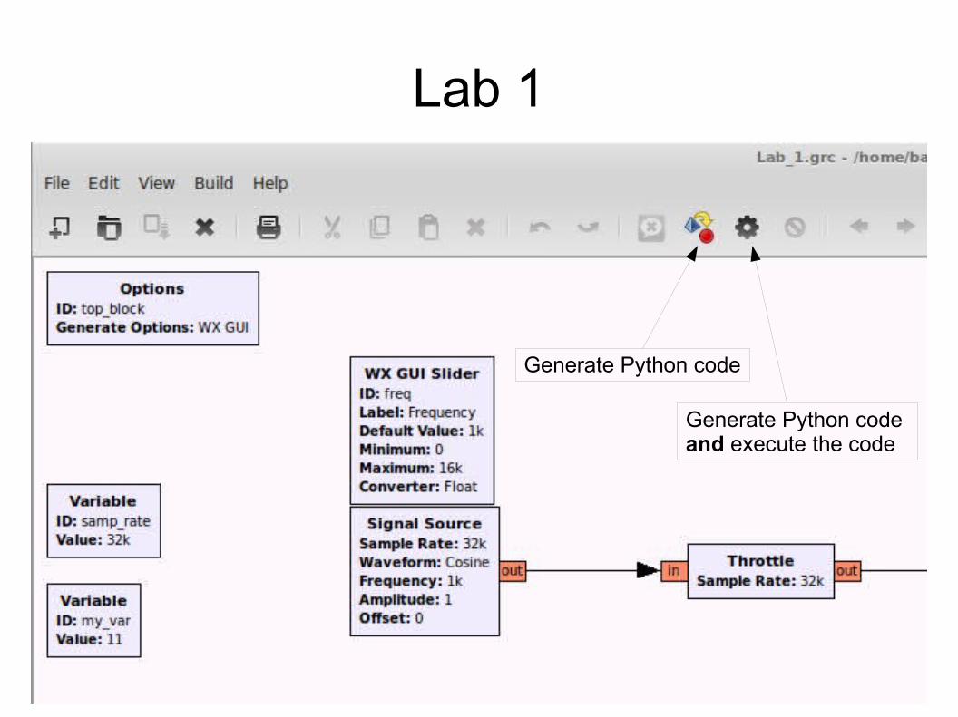
Lab 1

Generate Python code

Generate Python code and execute the code

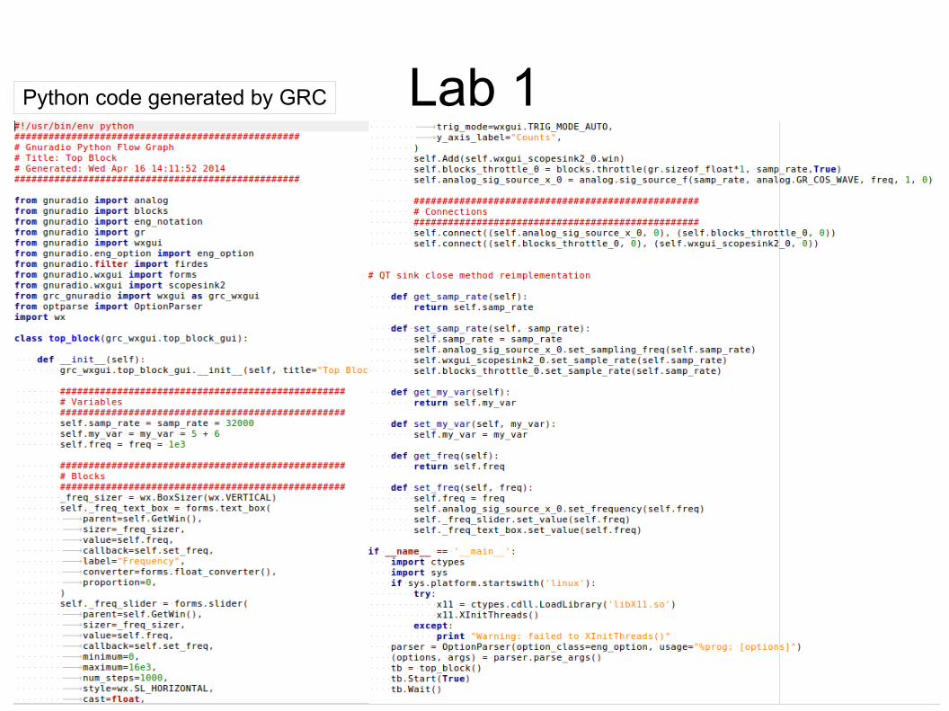
Lab 1Python code generated by GRC

Lab 1

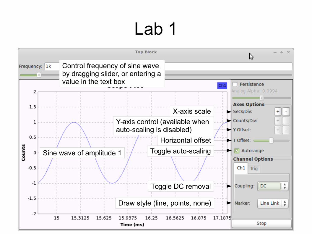
Sine wave of amplitude 1 Toggle auto-scaling

Horizontal offset

Y-axis control (available when auto-scaling is disabled)

X-axis scale

Toggle DC removal

Draw style (line, points, none)

Control frequency of sine wave by dragging slider, or entering a value in the text box

Lab 1

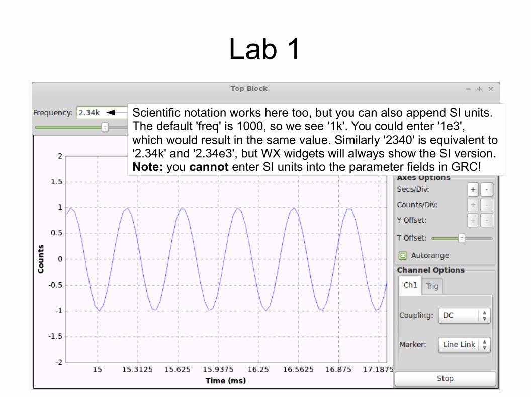
Scientific notation works here too, but you can also append SI units.The default 'freq' is 1000, so we see '1k'. You could enter '1e3', which would result in the same value. Similarly '2340' is equivalent to '2.34k' and '2.34e3', but WX widgets will always show the SI version.Note: you cannot enter SI units into the parameter fields in GRC!

Lab 1: TCP Client (producer)

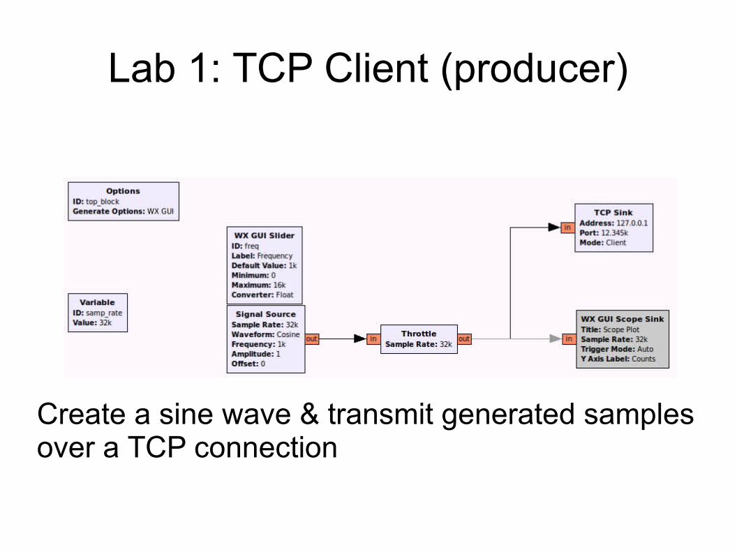
Create a sine wave & transmit generated samples over a TCP connection

Lab 1: TCP Client (producer)

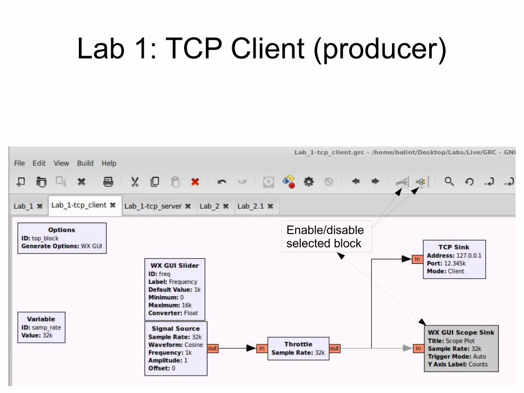
Enable/disable selected block

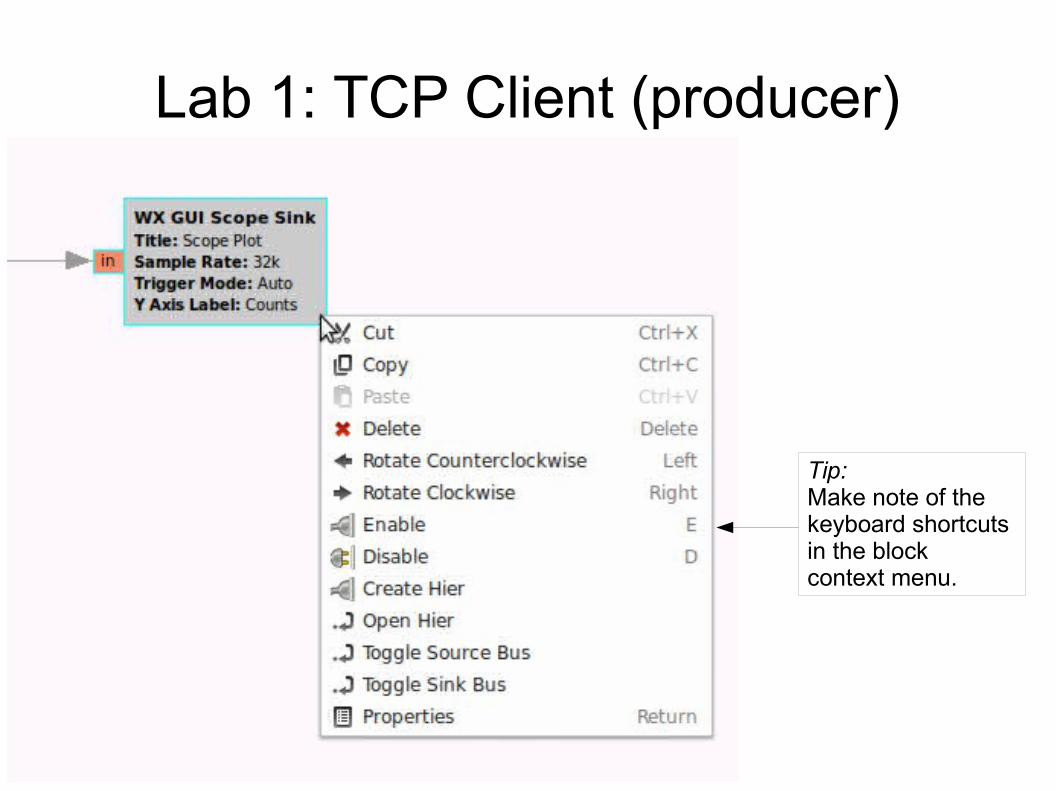
Lab 1: TCP Client (producer)

Tip:Make note of the keyboard shortcuts in the block context menu.

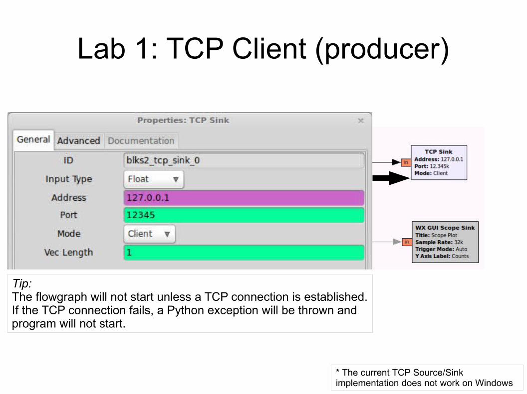
Lab 1: TCP Client (producer)

* The current TCP Source/Sink implementation does not work on Windows

Tip:The flowgraph will not start unless a TCP connection is established.If the TCP connection fails, a Python exception will be thrown and program will not start.

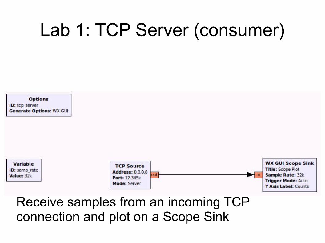
Lab 1: TCP Server (consumer)

Receive samples from an incoming TCP connection and plot on a Scope Sink

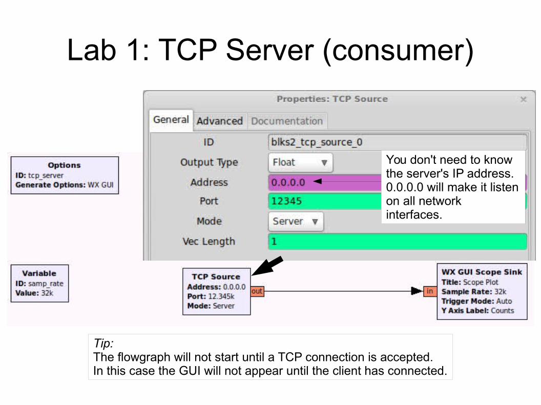
Lab 1: TCP Server (consumer)

Tip:The flowgraph will not start until a TCP connection is accepted.In this case the GUI will not appear until the client has connected.

You don't need to know the server's IP address. 0.0.0.0 will make it listen on all network interfaces.

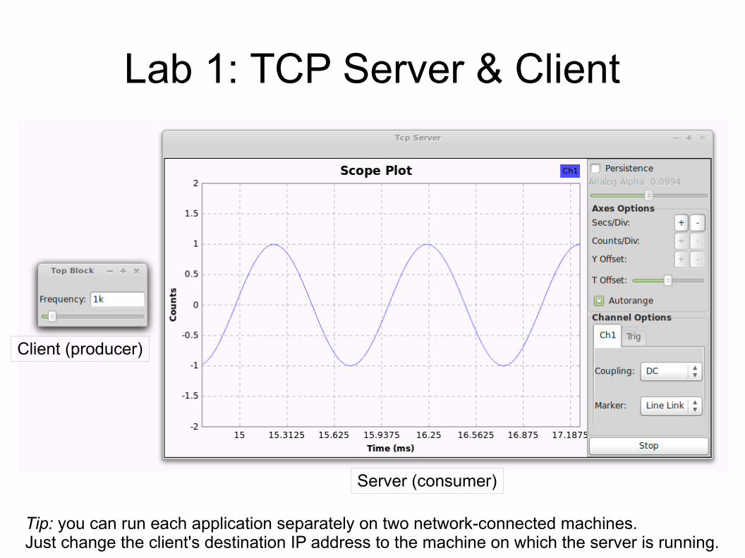
Lab 1: TCP Server & Client

Client (producer)

Server (consumer)

Tip: you can run each application separately on two network-connected machines.Just change the client's destination IP address to the machine on which the server is running.

Lab 2

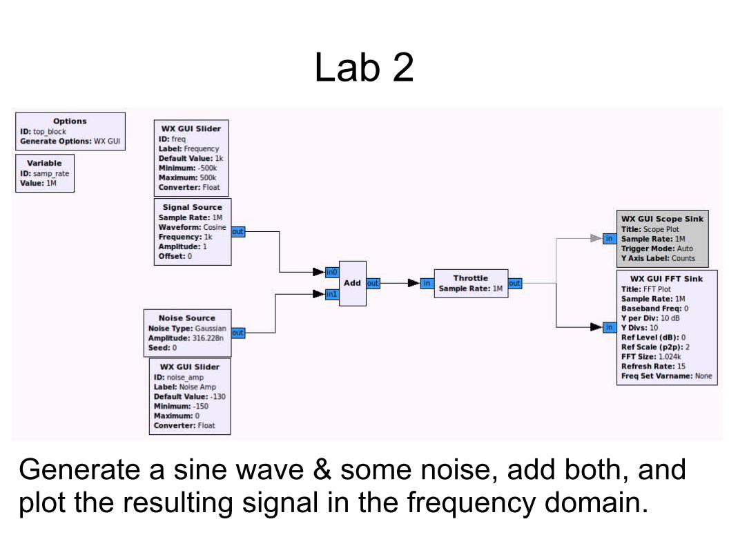
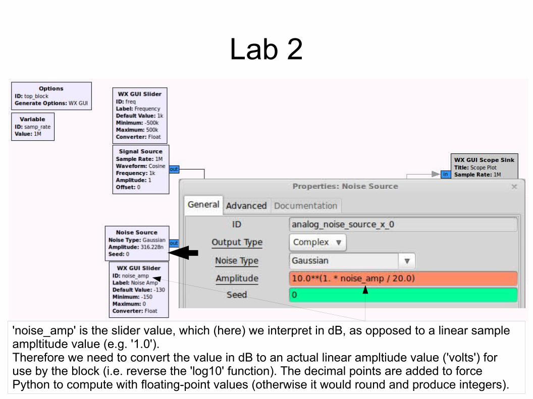
Generate a sine wave & some noise, add both, and plot the resulting signal in the frequency domain.

Lab 2

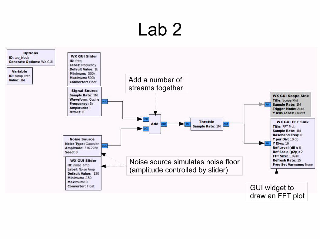
Noise source simulates noise floor(amplitude controlled by slider)

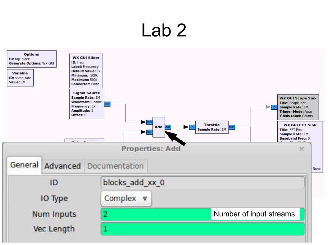
Add a number of streams together

GUI widget todraw an FFT plot

Lab 2

Lab 2

'noise_amp' is the slider value, which (here) we interpret in dB, as opposed to a linear sample ampltitude value (e.g. '1.0').Therefore we need to convert the value in dB to an actual linear ampltiude value ('volts') for use by the block (i.e. reverse the 'log10' function). The decimal points are added to force Python to compute with floating-point values (otherwise it would round and produce integers).

Lab 2

Number of input streams

Lab 2

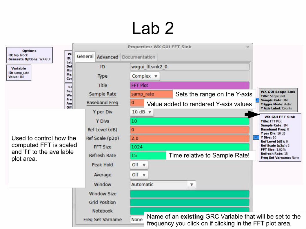
Sets the range on the Y-axis

Value added to rendered Y-axis values

Used to control how the computed FFT is scaled and 'fit' to the available plot area.

Name of an existing GRC Variable that will be set to the frequency you click on if clicking in the FFT plot area.

Time relative to Sample Rate!

Lab 2

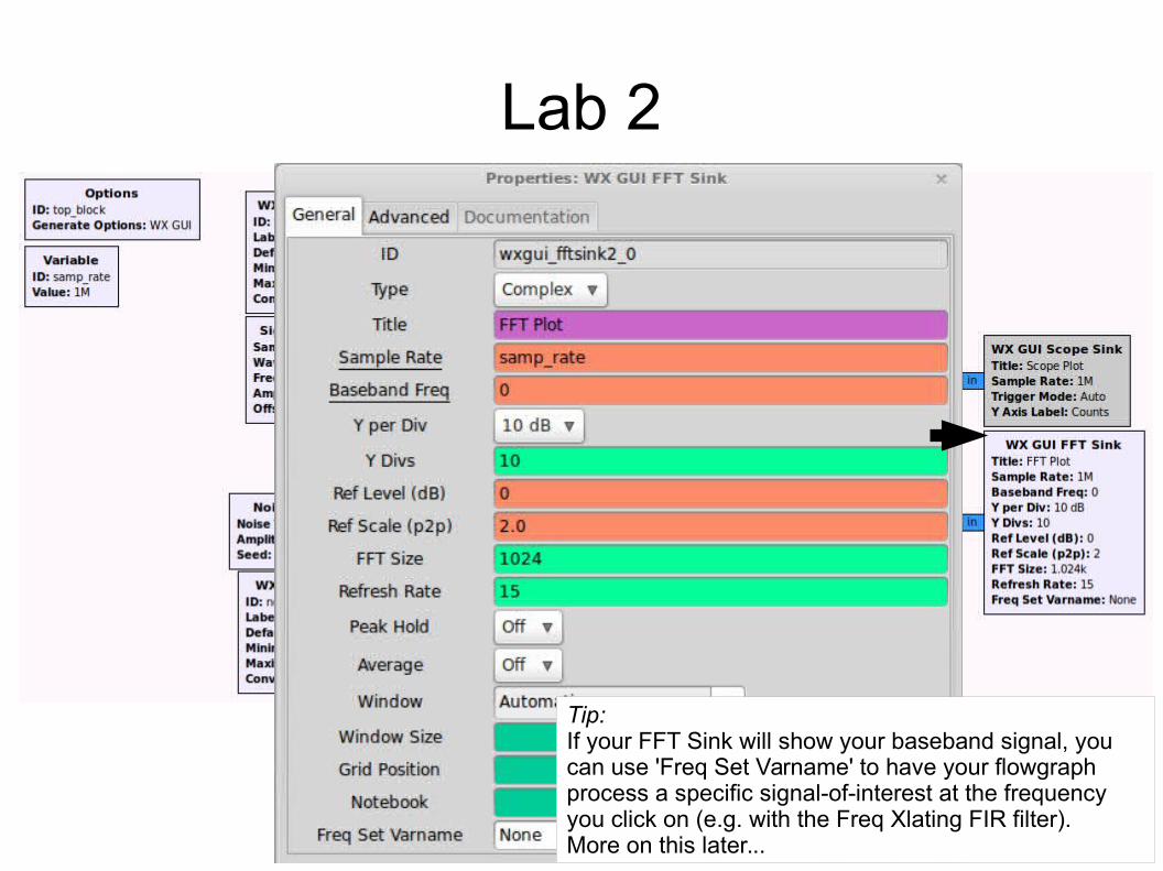
Tip:If your FFT Sink will show your baseband signal, you can use 'Freq Set Varname' to have your flowgraph process a specific signal-of-interest at the frequency you click on (e.g. with the Freq Xlating FIR filter).More on this later...

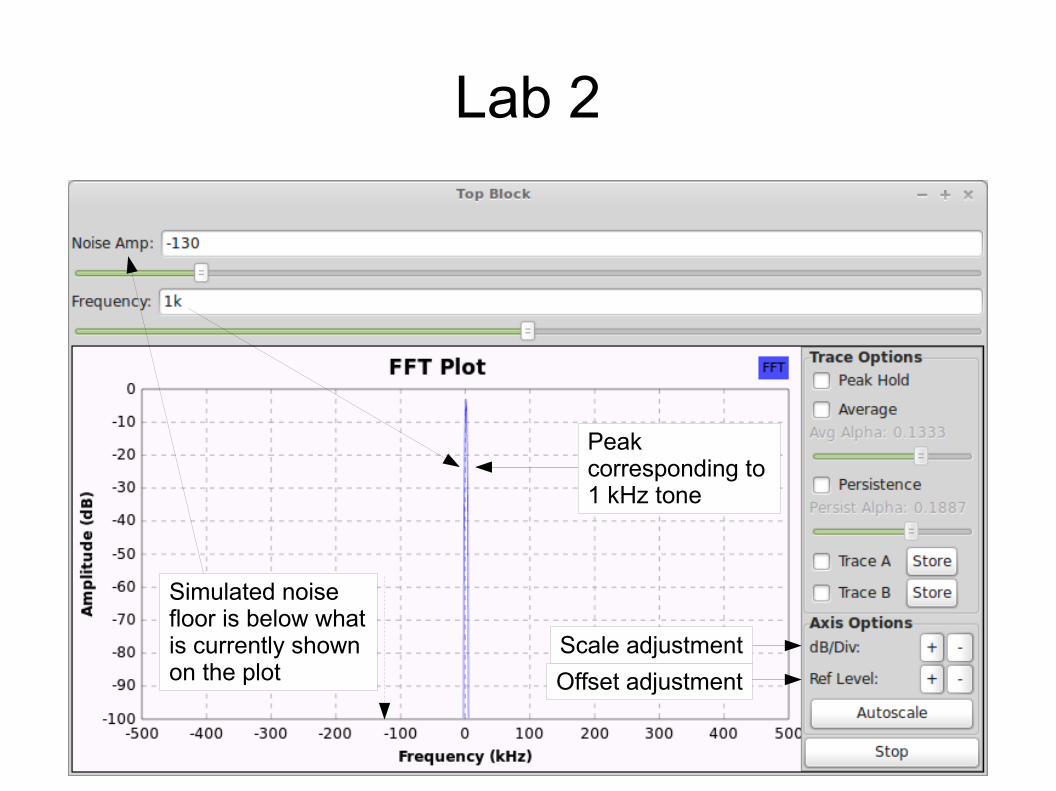
Lab 2

Scale adjustment

Offset adjustment

Peak corresponding to 1 kHz tone

Simulated noise floor is below what is currently shown on the plot

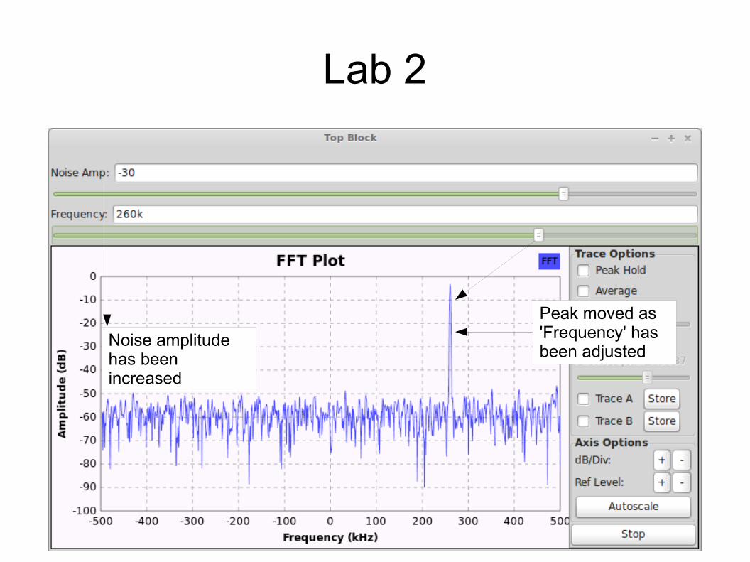
Lab 2

Peak moved as 'Frequency' has been adjusted

Noise amplitude has been increased

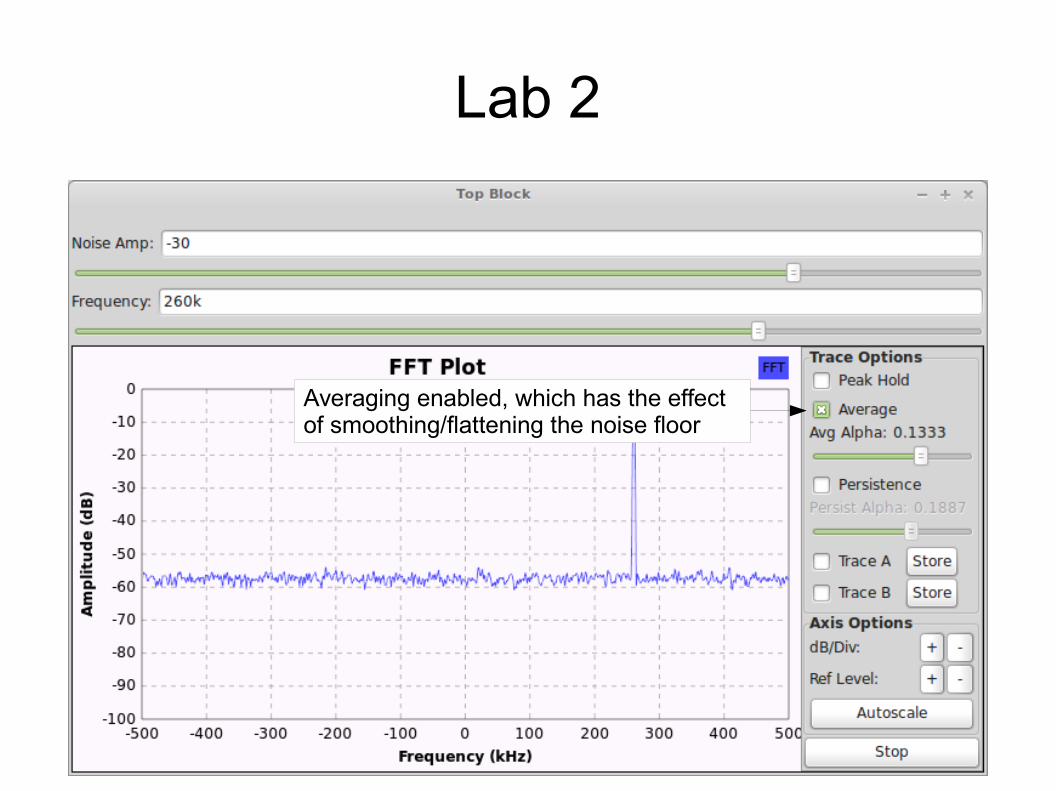
Lab 2

Averaging enabled, which has the effect of smoothing/flattening the noise floor

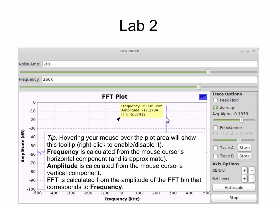
Lab 2

Tip: Hovering your mouse over the plot area will show this tooltip (right-click to enable/disable it).Frequency is calculated from the mouse cursor's horizontal component (and is approximate).Amplitude is calculated from the mouse cursor's vertical component.FFT is calculated from the amplitude of the FFT bin that corresponds to Frequency.

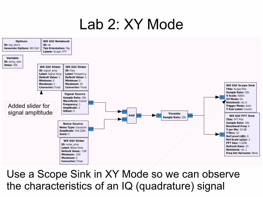
Lab 2: XY Mode

Use a Scope Sink in XY Mode so we can observe the characteristics of an IQ (quadrature) signal

Added slider for signal ampltitude

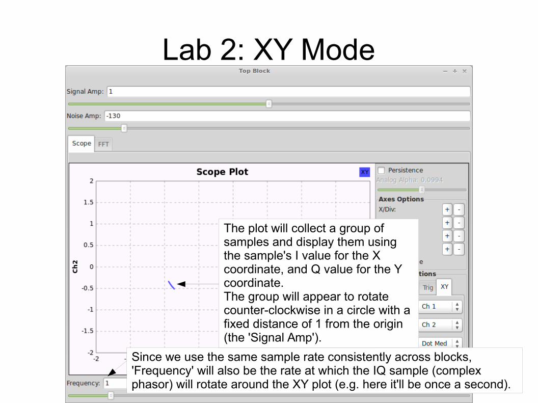
Lab 2: XY Mode

Since we use the same sample rate consistently across blocks, 'Frequency' will also be the rate at which the IQ sample (complex phasor) will rotate around the XY plot (e.g. here it'll be once a second).

The plot will collect a group of samples and display them using the sample's I value for the X coordinate, and Q value for the Y coordinate.The group will appear to rotate counter-clockwise in a circle with a fixed distance of 1 from the origin (the 'Signal Amp').

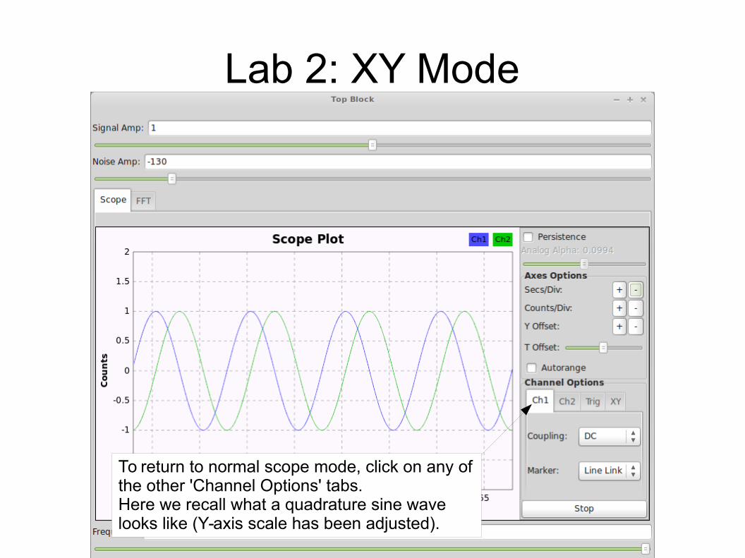
Lab 2: XY Mode

To return to normal scope mode, click on any of the other 'Channel Options' tabs.Here we recall what a quadrature sine wave looks like (Y-axis scale has been adjusted).

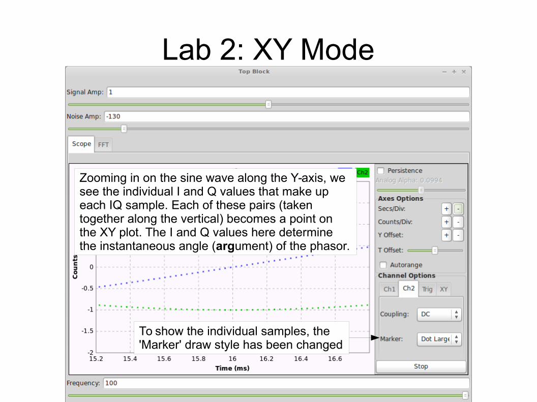
Lab 2: XY Mode

Zooming in on the sine wave along the Y-axis, we see the individual I and Q values that make up each IQ sample. Each of these pairs (taken together along the vertical) becomes a point on the XY plot. The I and Q values here determine the instantaneous angle (argument) of the phasor.

To show the individual samples, the 'Marker' draw style has been changed

Lab 2: XY Mode

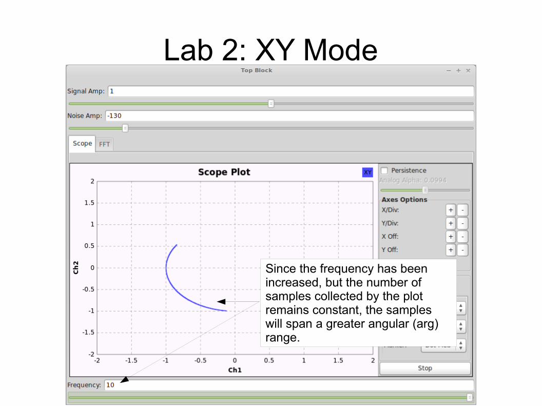
Since the frequency has been increased, but the number of samples collected by the plot remains constant, the samples will span a greater angular (arg) range.

Lab 2: XY Mode

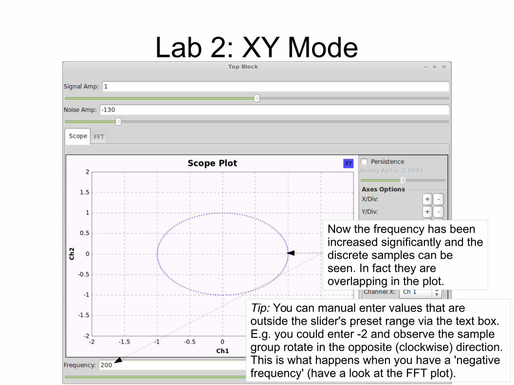
Now the frequency has been increased significantly and the discrete samples can be seen. In fact they are overlapping in the plot.

Tip: You can manual enter values that are outside the slider's preset range via the text box.E.g. you could enter -2 and observe the sample group rotate in the opposite (clockwise) direction. This is what happens when you have a 'negative frequency' (have a look at the FFT plot).

Lab 2: XY Mode

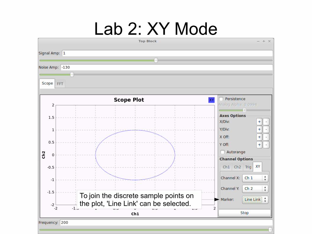
To join the discrete sample points on the plot, 'Line Link' can be selected.

Lab 2: XY Mode

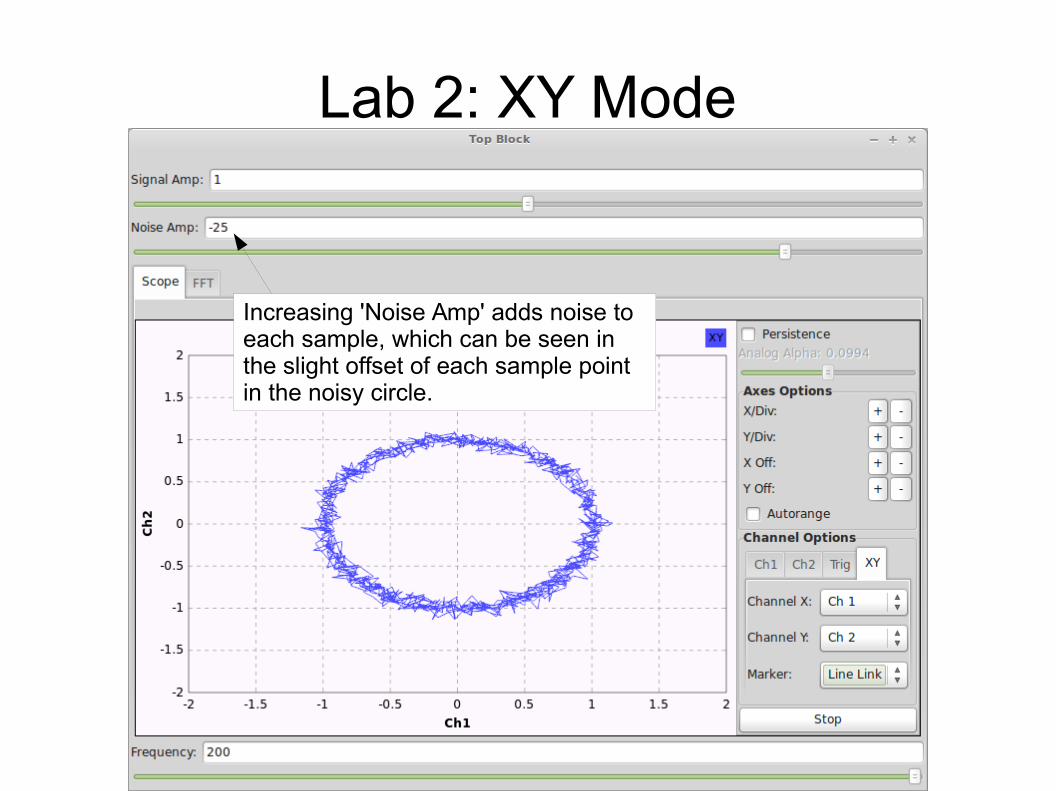
Increasing 'Noise Amp' adds noise to each sample, which can be seen in the slight offset of each sample point in the noisy circle.

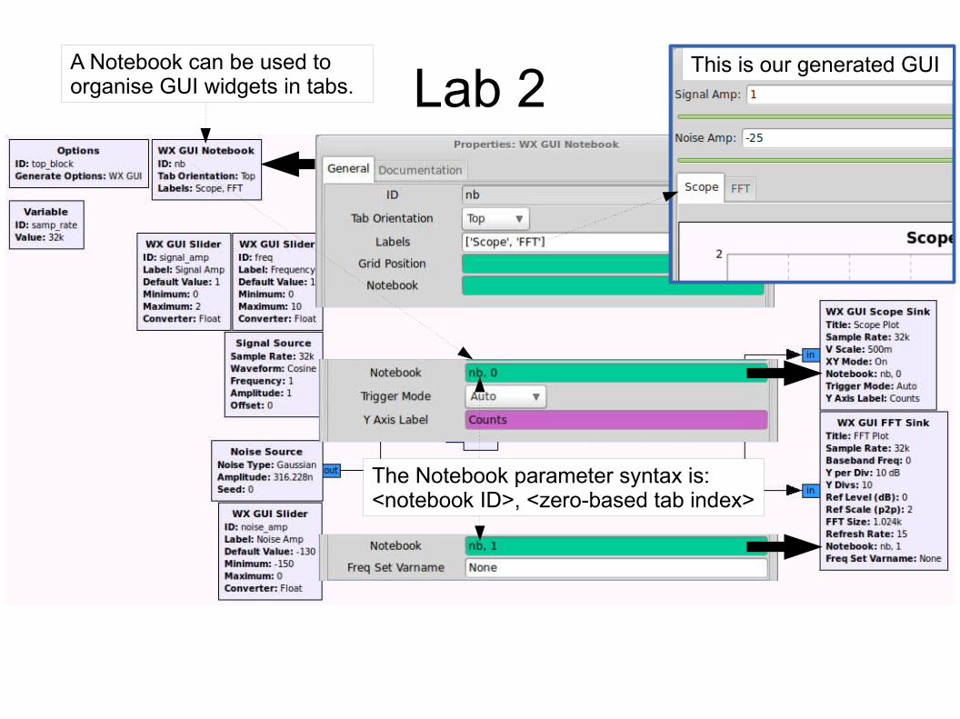
Lab 2A Notebook can be used to organise GUI widgets in tabs.

The Notebook parameter syntax is: <notebook ID>, <zero-based tab index>

This is our generated GUI

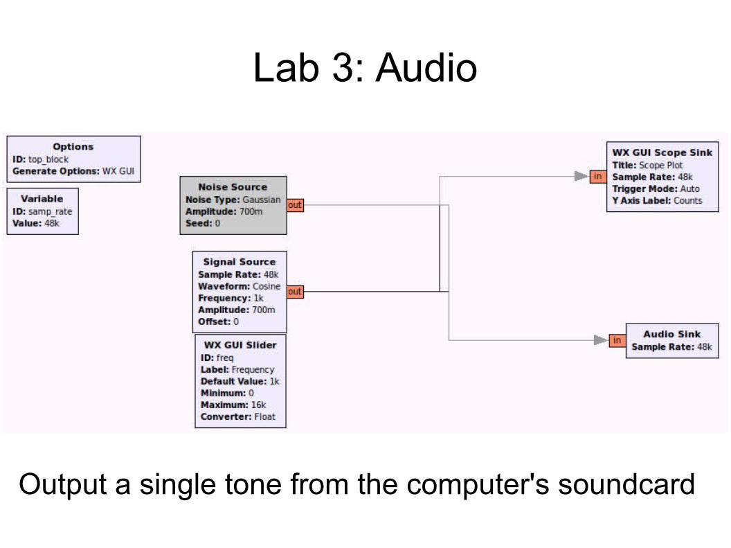
Lab 3: Audio

Output a single tone from the computer's soundcard

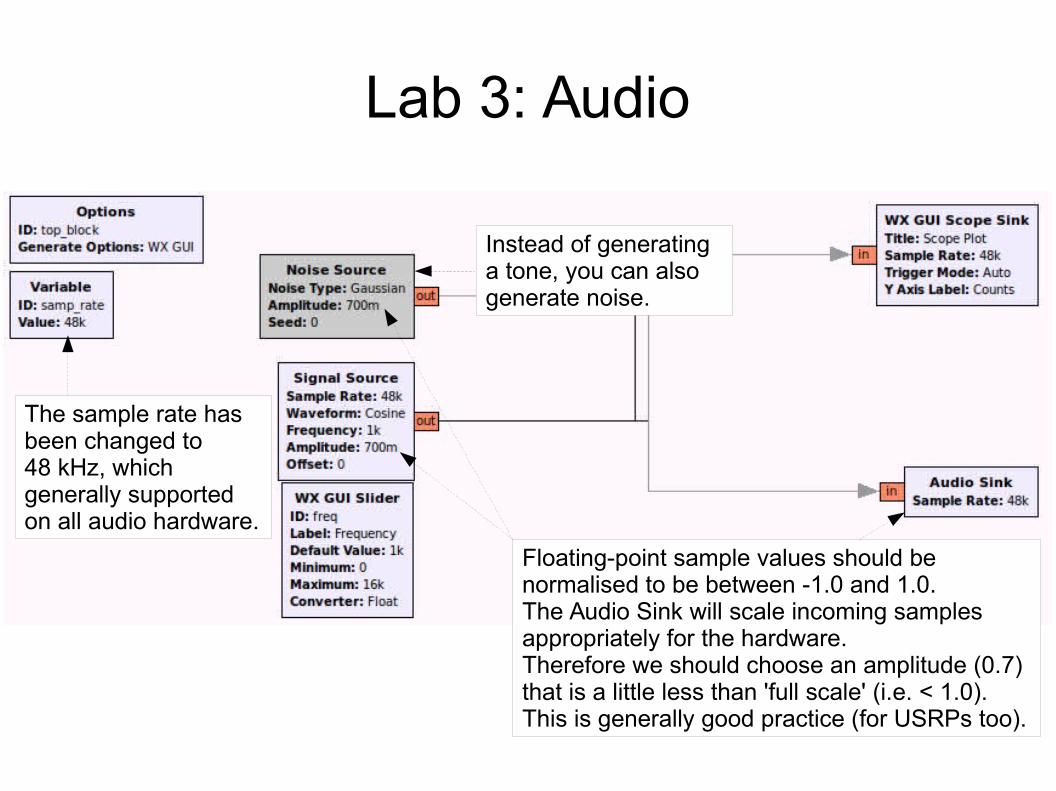
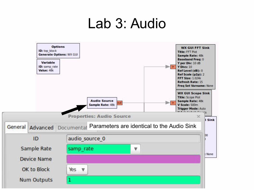
Lab 3: Audio

The sample rate has been changed to 48 kHz, which generally supported on all audio hardware.

Instead of generating a tone, you can also generate noise.

Floating-point sample values should be normalised to be between -1.0 and 1.0.The Audio Sink will scale incoming samples appropriately for the hardware.Therefore we should choose an amplitude (0.7) that is a little less than 'full scale' (i.e. < 1.0).This is generally good practice (for USRPs too).

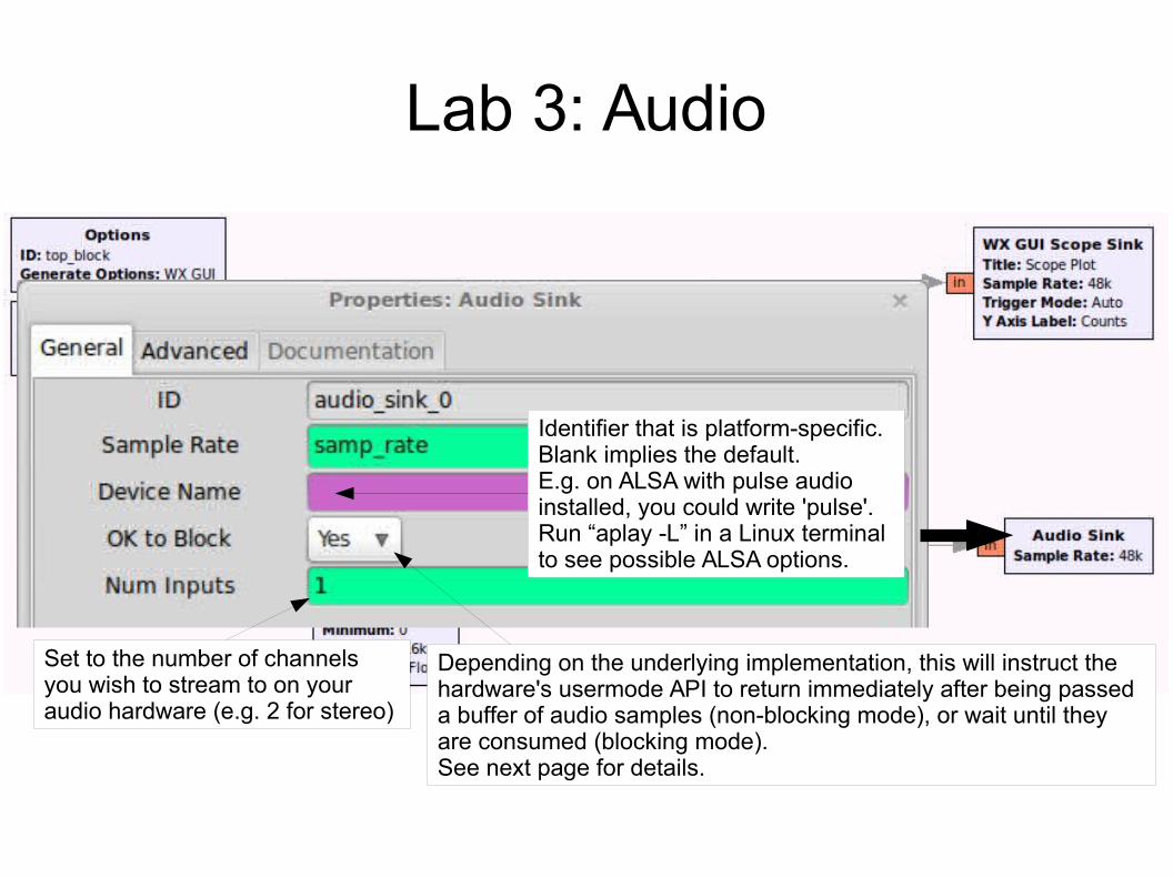
Lab 3: Audio

Identifier that is platform-specific. Blank implies the default. E.g. on ALSA with pulse audio installed, you could write 'pulse'.Run “aplay -L” in a Linux terminal to see possible ALSA options.

Set to the number of channels you wish to stream to on your audio hardware (e.g. 2 for stereo)

Depending on the underlying implementation, this will instruct the hardware's usermode API to return immediately after being passed a buffer of audio samples (non-blocking mode), or wait until they are consumed (blocking mode).See next page for details.

Lab 3: Audio

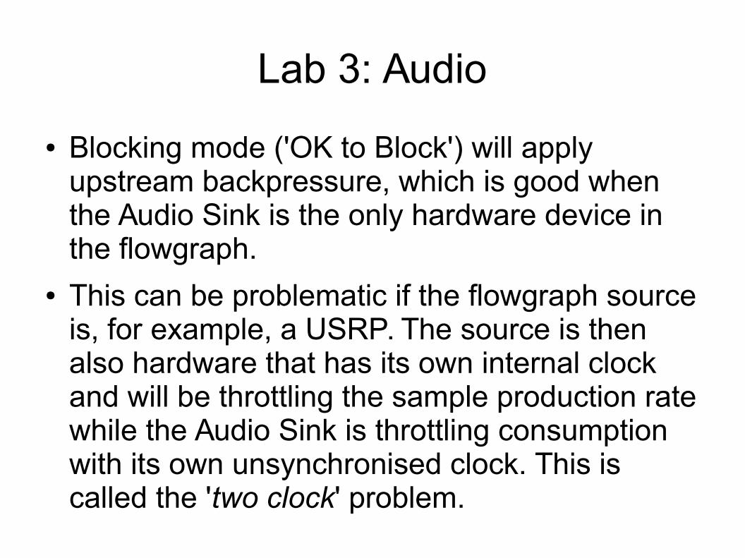
● Blocking mode ('OK to Block') will apply upstream backpressure, which is good when the Audio Sink is the only hardware device in the flowgraph.

● This can be problematic if the flowgraph source is, for example, a USRP. The source is then also hardware that has its own internal clock and will be throttling the sample production rate while the Audio Sink is throttling consumption with its own unsynchronised clock. This is called the 'two clock' problem.

Lab 3: Audio

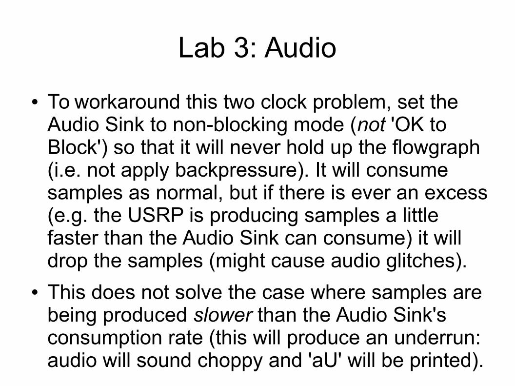
● To workaround this two clock problem, set the Audio Sink to non-blocking mode (not 'OK to Block') so that it will never hold up the flowgraph (i.e. not apply backpressure). It will consume samples as normal, but if there is ever an excess (e.g. the USRP is producing samples a little faster than the Audio Sink can consume) it will drop the samples (might cause audio glitches).

● This does not solve the case where samples are being produced slower than the Audio Sink's consumption rate (this will produce an underrun: audio will sound choppy and 'aU' will be printed).

Lab 3: Audio

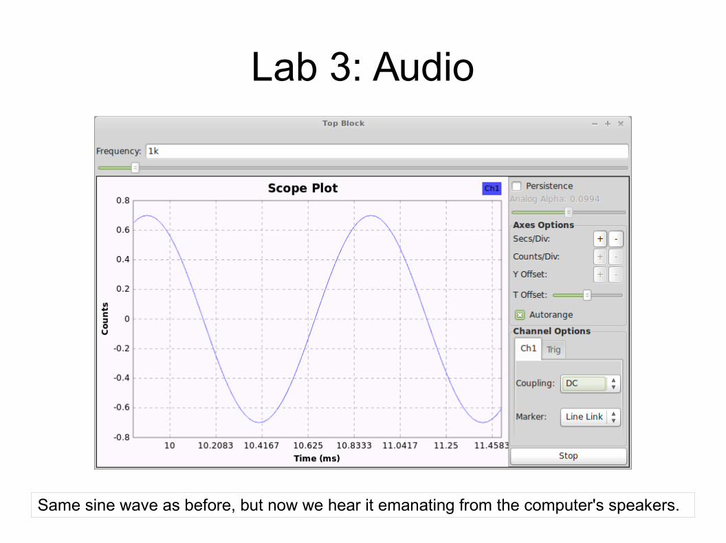
Same sine wave as before, but now we hear it emanating from the computer's speakers.

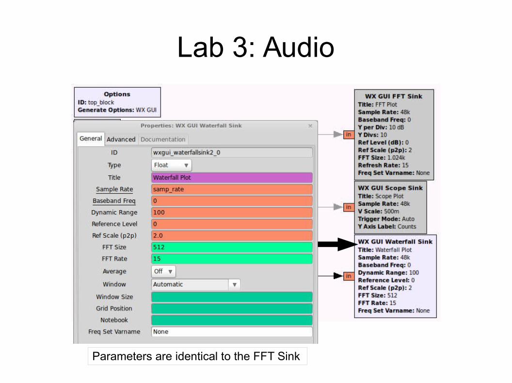
Lab 3: Audio

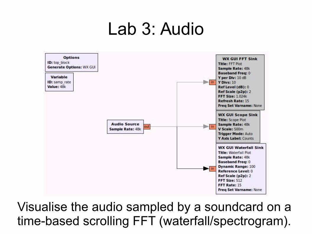
Visualise the audio sampled by a soundcard on a time-based scrolling FFT (waterfall/spectrogram).

Lab 3: Audio

Parameters are identical to the Audio Sink

Lab 3: Audio

Parameters are identical to the FFT Sink

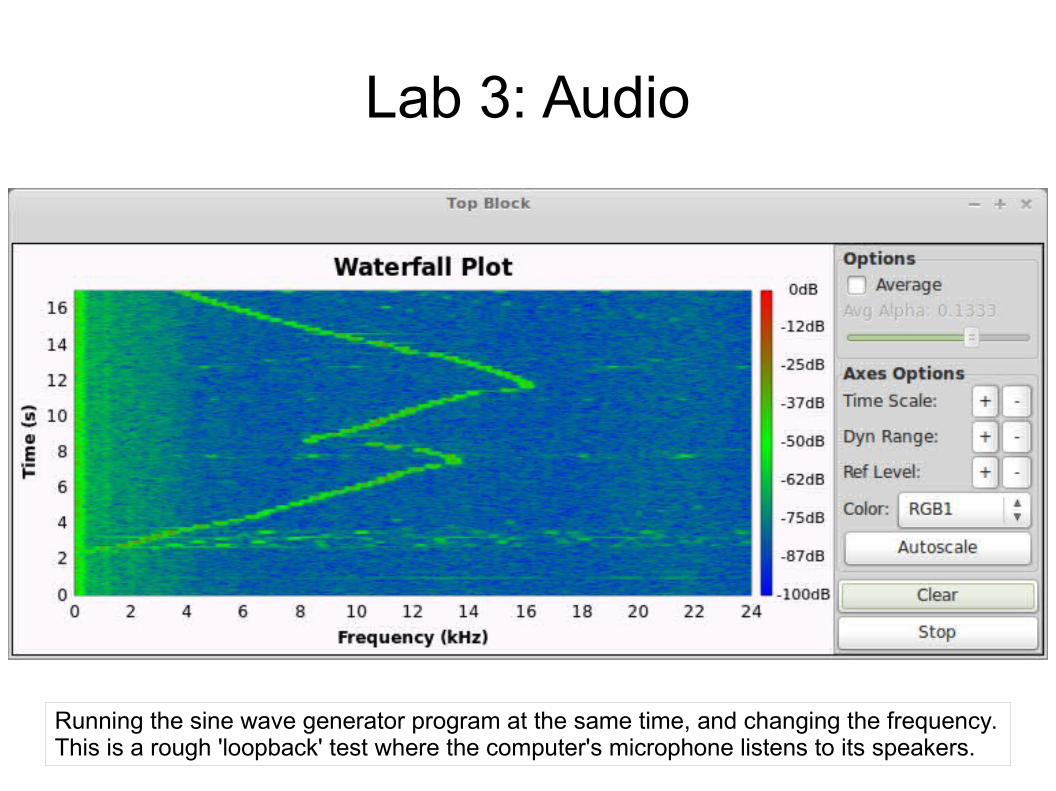
Lab 3: Audio

Running the sine wave generator program at the same time, and changing the frequency.This is a rough 'loopback' test where the computer's microphone listens to its speakers.

Lab 4: FM RX

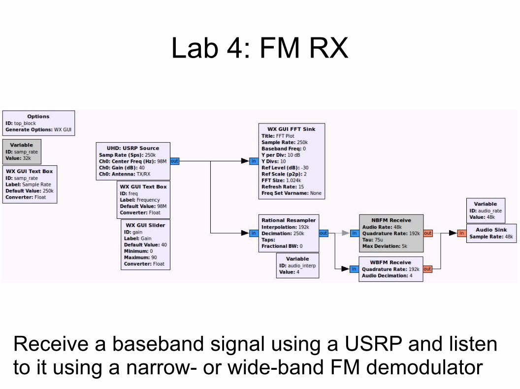
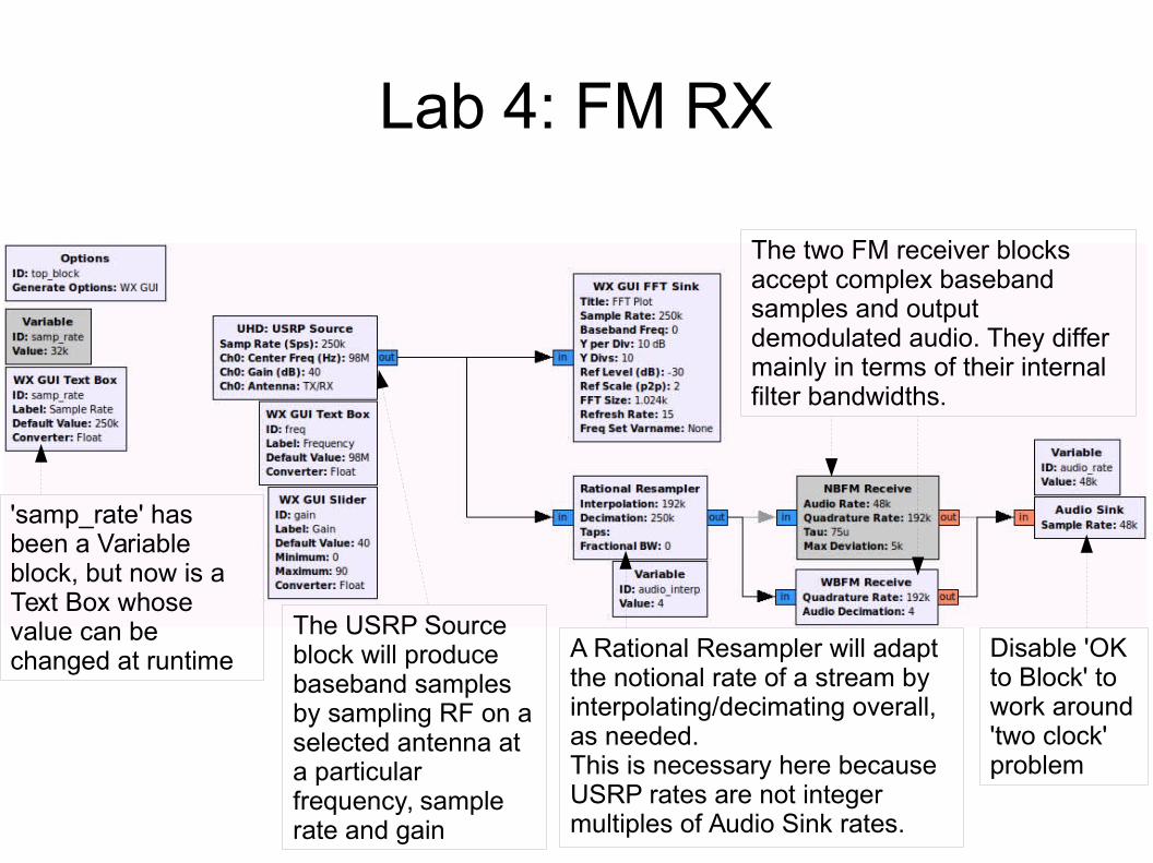
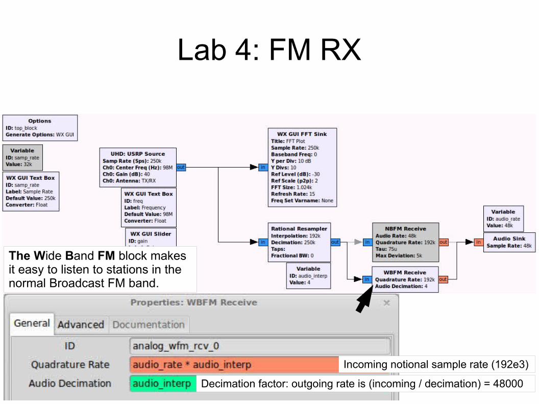
Receive a baseband signal using a USRP and listen to it using a narrow- or wide-band FM demodulator

Lab 4: FM RX

'samp_rate' has been a Variable block, but now is a Text Box whose value can be changed at runtime

The USRP Source block will produce baseband samples by sampling RF on a selected antenna at a particular frequency, sample rate and gain

A Rational Resampler will adapt the notional rate of a stream by interpolating/decimating overall, as needed.This is necessary here because USRP rates are not integer multiples of Audio Sink rates.

The two FM receiver blocks accept complex baseband samples and output demodulated audio. They differ mainly in terms of their internal filter bandwidths.

Disable 'OK to Block' to work around 'two clock' problem

Lab 4: FM RX

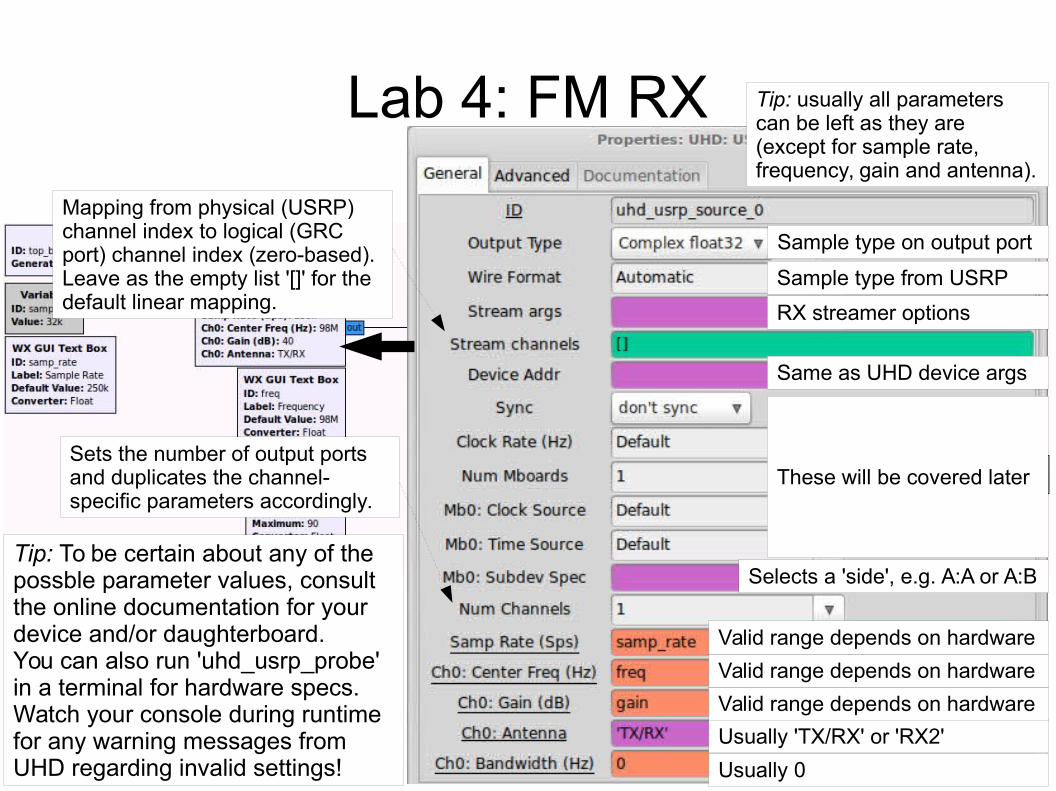
Usually 'TX/RX' or 'RX2'

Tip: To be certain about any of the possble parameter values, consult the online documentation for your device and/or daughterboard.You can also run 'uhd_usrp_probe' in a terminal for hardware specs.Watch your console during runtime for any warning messages from UHD regarding invalid settings! Usually 0

Valid range depends on hardware

Valid range depends on hardware

Valid range depends on hardware

Sample type on output port

Sample type from USRP

Same as UHD device args

RX streamer options

Mapping from physical (USRP) channel index to logical (GRC port) channel index (zero-based). Leave as the empty list '[]' for the default linear mapping.

Tip: usually all parameters can be left as they are (except for sample rate, frequency, gain and antenna).

These will be covered later

Selects a 'side', e.g. A:A or A:B

Sets the number of output ports and duplicates the channel-specific parameters accordingly.

Lab 4: FM RX

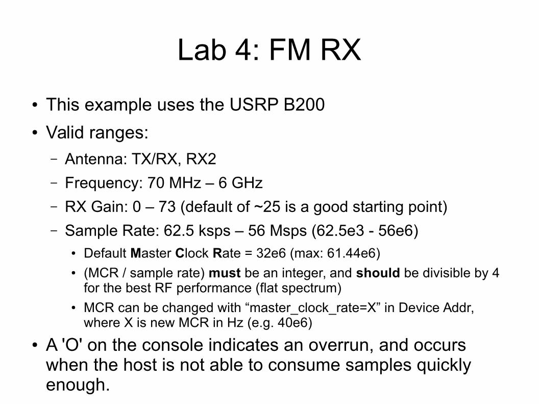
● This example uses the USRP B200● Valid ranges:

– Antenna: TX/RX, RX2

– Frequency: 70 MHz – 6 GHz

– RX Gain: 0 – 73 (default of ~25 is a good starting point)

– Sample Rate: 62.5 ksps – 56 Msps (62.5e3 - 56e6)● Default Master Clock Rate = 32e6 (max: 61.44e6)● (MCR / sample rate) must be an integer, and should be divisible by 4

for the best RF performance (flat spectrum)● MCR can be changed with “master_clock_rate=X” in Device Addr,

where X is new MCR in Hz (e.g. 40e6)

● A 'O' on the console indicates an overrun, and occurs when the host is not able to consume samples quickly enough.

Lab 4: FM RX

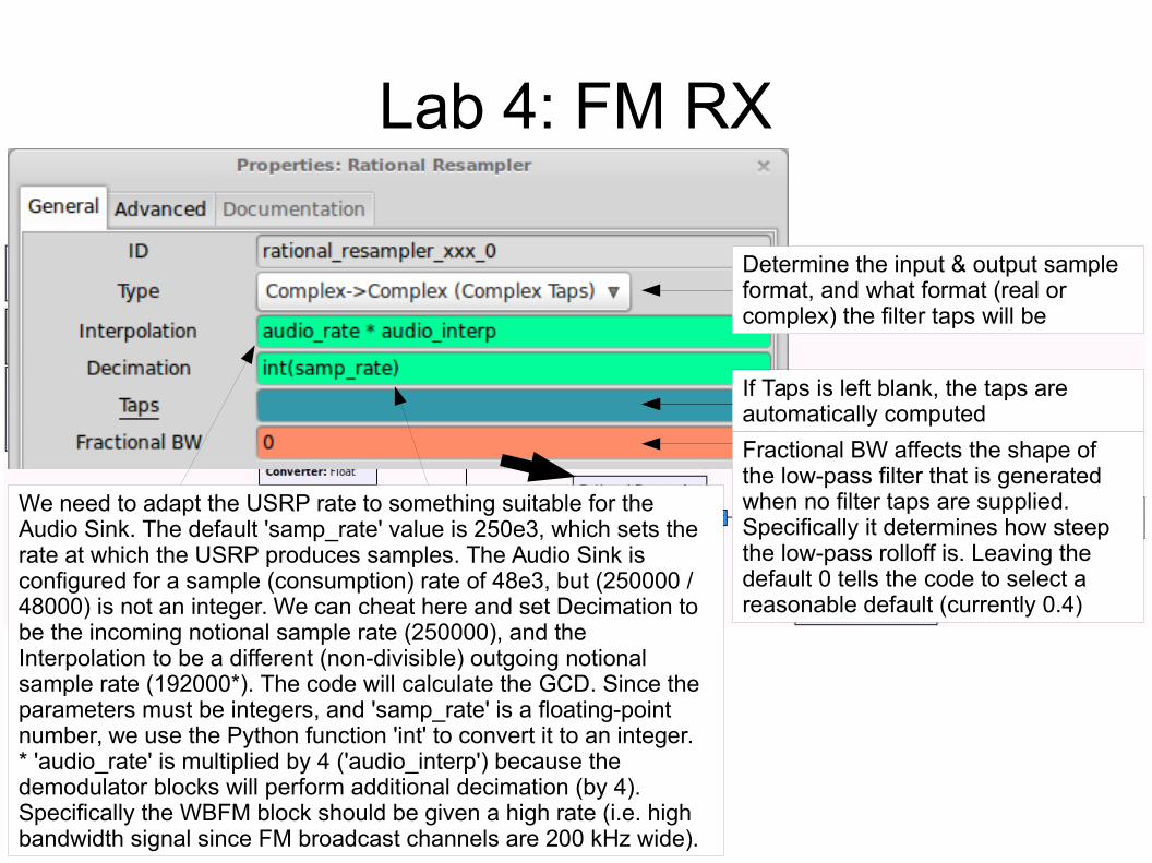
Determine the input & output sample format, and what format (real or complex) the filter taps will be

If Taps is left blank, the taps are automatically computed

Fractional BW affects the shape of the low-pass filter that is generated when no filter taps are supplied.Specifically it determines how steep the low-pass rolloff is. Leaving the default 0 tells the code to select a reasonable default (currently 0.4)

We need to adapt the USRP rate to something suitable for the Audio Sink. The default 'samp_rate' value is 250e3, which sets the rate at which the USRP produces samples. The Audio Sink is configured for a sample (consumption) rate of 48e3, but (250000 / 48000) is not an integer. We can cheat here and set Decimation to be the incoming notional sample rate (250000), and the Interpolation to be a different (non-divisible) outgoing notional sample rate (192000*). The code will calculate the GCD. Since the parameters must be integers, and 'samp_rate' is a floating-point number, we use the Python function 'int' to convert it to an integer. * 'audio_rate' is multiplied by 4 ('audio_interp') because the demodulator blocks will perform additional decimation (by 4). Specifically the WBFM block should be given a high rate (i.e. high bandwidth signal since FM broadcast channels are 200 kHz wide).

Lab 4: FM RX

The Wide Band FM block makes it easy to listen to stations in the normal Broadcast FM band.

Incoming notional sample rate (192e3)

Decimation factor: outgoing rate is (incoming / decimation) = 48000

Lab 4: FM RX

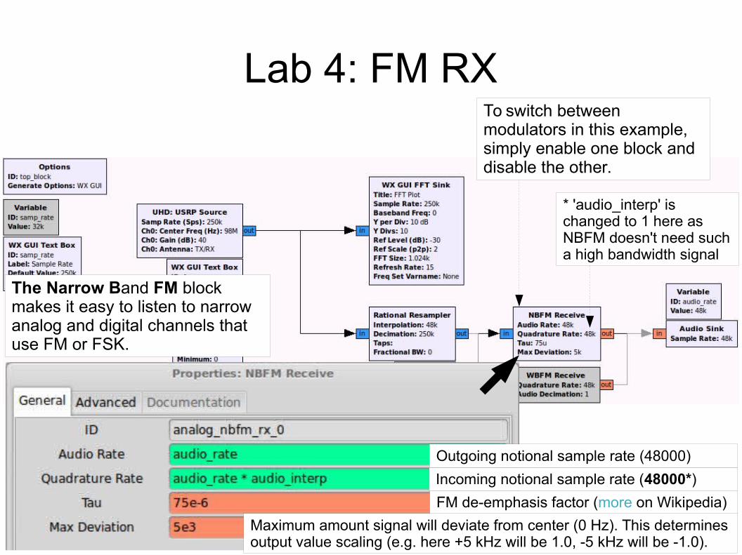
The Narrow Band FM block makes it easy to listen to narrow analog and digital channels that use FM or FSK.

Incoming notional sample rate (48000*)

Outgoing notional sample rate (48000)

To switch between modulators in this example, simply enable one block and disable the other.

FM de-emphasis factor (more on Wikipedia)

Maximum amount signal will deviate from center (0 Hz). This determines output value scaling (e.g. here +5 kHz will be 1.0, -5 kHz will be -1.0).

* 'audio_interp' is changed to 1 here as NBFM doesn't need such a high bandwidth signal

Lab 4: FM RX

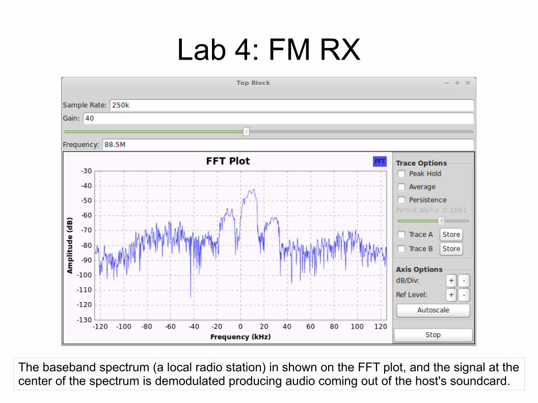
The baseband spectrum (a local radio station) in shown on the FFT plot, and the signal at the center of the spectrum is demodulated producing audio coming out of the host's soundcard.

Lab 4: Manual FM RX

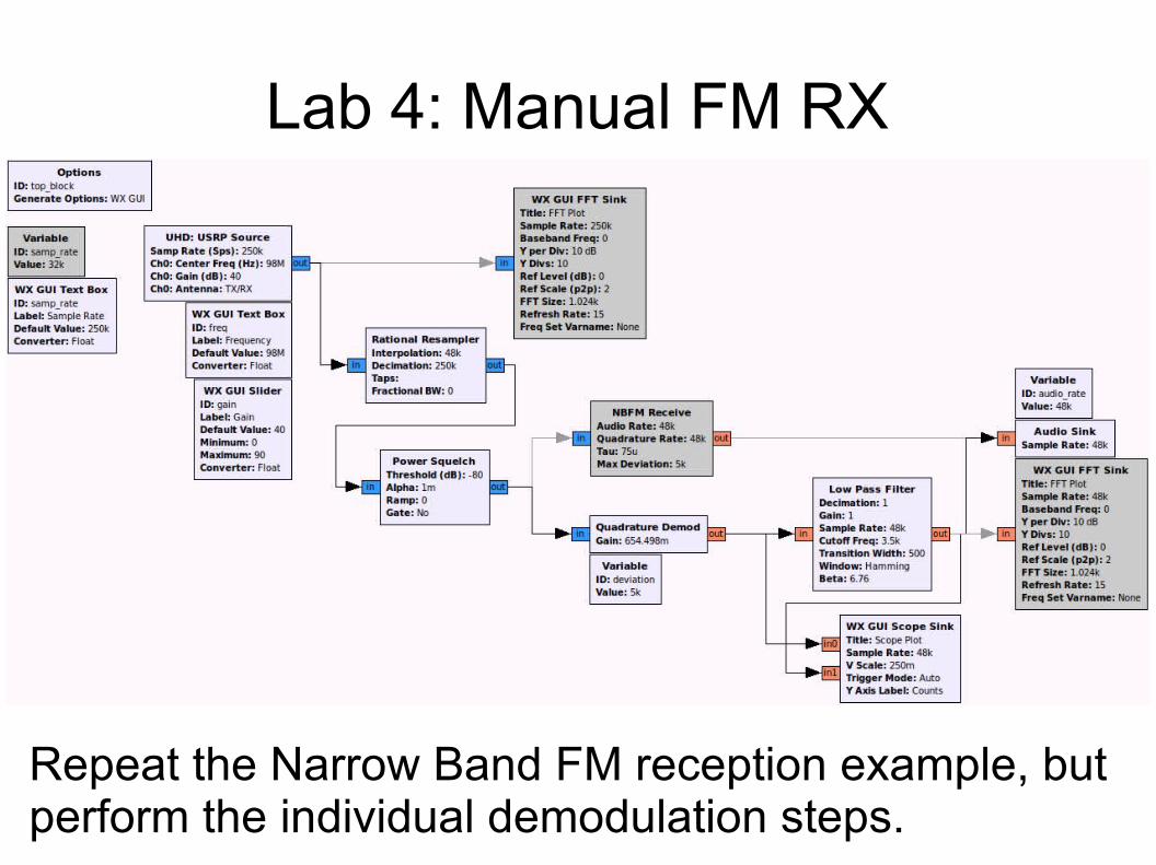
Repeat the Narrow Band FM reception example, but perform the individual demodulation steps.

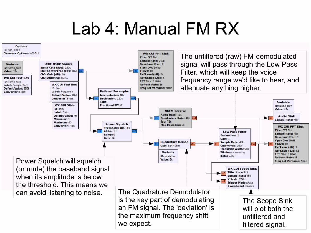
Lab 4: Manual FM RX

Power Squelch will squelch (or mute) the baseband signal when its amplitude is below the threshold. This means we can avoid listening to noise. The Quadrature Demodulator

is the key part of demodulating an FM signal. The 'deviation' is the maximum frequency shift we expect.

The unfiltered (raw) FM-demodulated signal will pass through the Low Pass Filter, which will keep the voice frequency range we'd like to hear, and attenuate anything higher.

The Scope Sink will plot both the unfiltered and filtered signal.

Lab 4: Manual FM RX

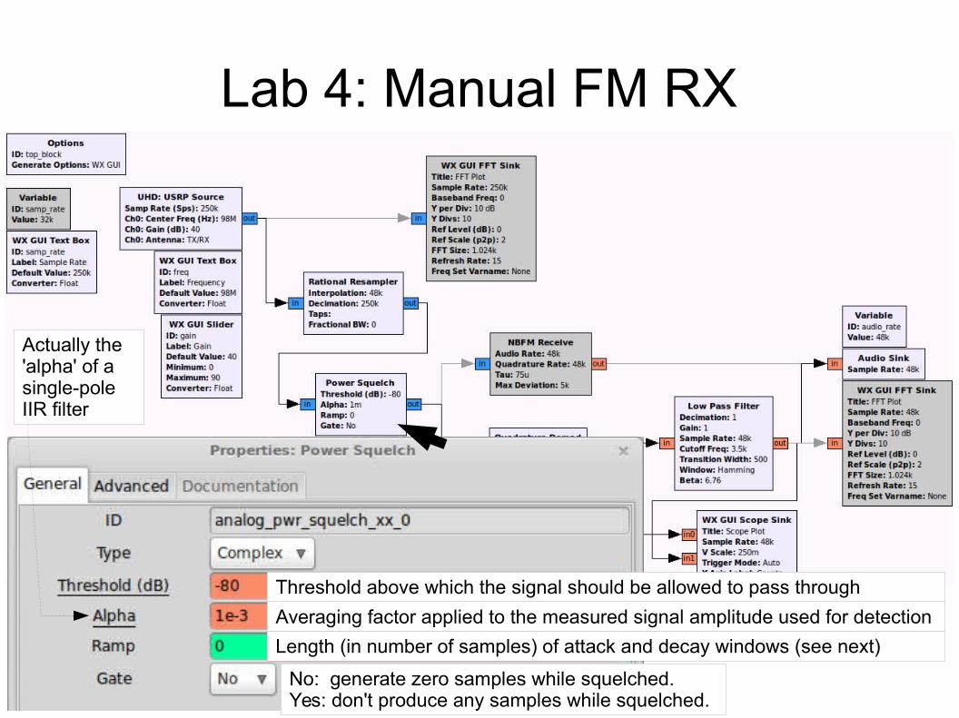
Threshold above which the signal should be allowed to pass through

Averaging factor applied to the measured signal amplitude used for detection

No: generate zero samples while squelched. Yes: don't produce any samples while squelched.

Actually the 'alpha' of a single-pole IIR filter

Length (in number of samples) of attack and decay windows (see next)

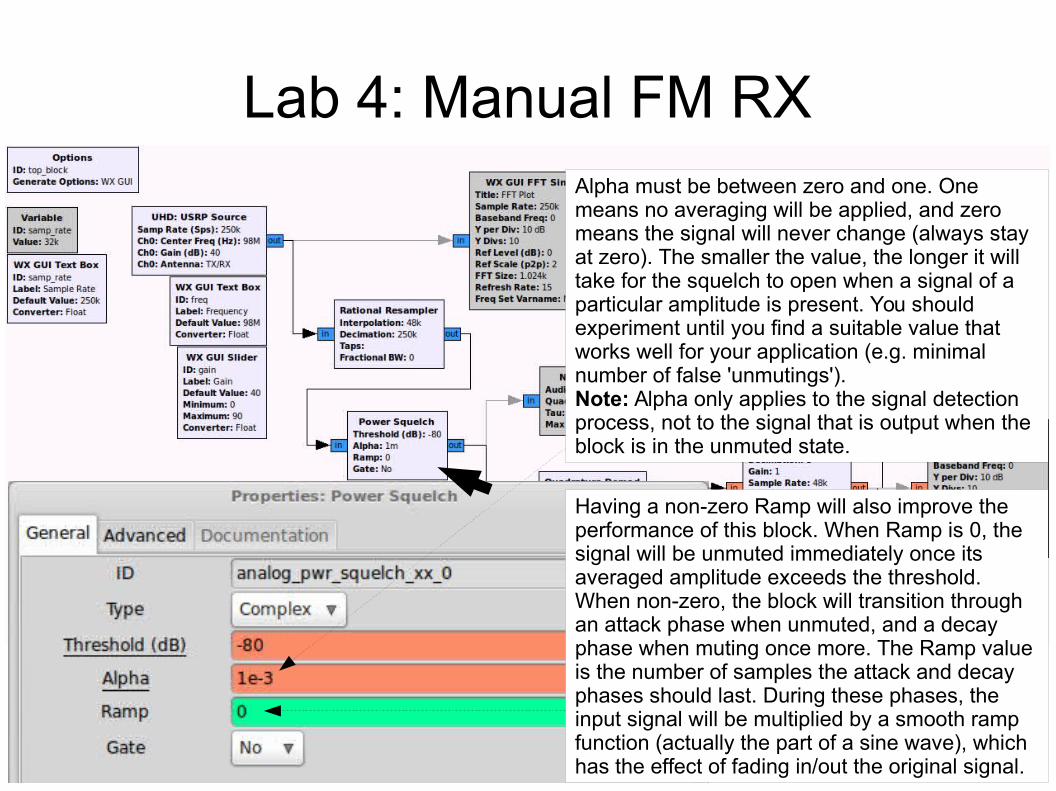
Lab 4: Manual FM RXAlpha must be between zero and one. One means no averaging will be applied, and zero means the signal will never change (always stay at zero). The smaller the value, the longer it will take for the squelch to open when a signal of a particular amplitude is present. You should experiment until you find a suitable value that works well for your application (e.g. minimal number of false 'unmutings').Note: Alpha only applies to the signal detection process, not to the signal that is output when the block is in the unmuted state.

Having a non-zero Ramp will also improve the performance of this block. When Ramp is 0, the signal will be unmuted immediately once its averaged amplitude exceeds the threshold. When non-zero, the block will transition through an attack phase when unmuted, and a decay phase when muting once more. The Ramp value is the number of samples the attack and decay phases should last. During these phases, the input signal will be multiplied by a smooth ramp function (actually the part of a sine wave), which has the effect of fading in/out the original signal.

Lab 4: Manual FM RX

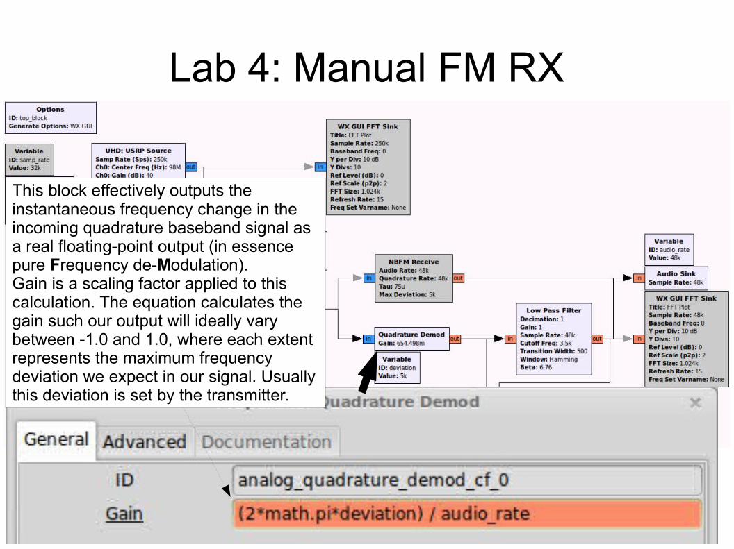
This block effectively outputs the instantaneous frequency change in the incoming quadrature baseband signal as a real floating-point output (in essence pure Frequency de-Modulation).Gain is a scaling factor applied to this calculation. The equation calculates the gain such our output will ideally vary between -1.0 and 1.0, where each extent represents the maximum frequency deviation we expect in our signal. Usually this deviation is set by the transmitter.

Lab 4: Manual FM RX

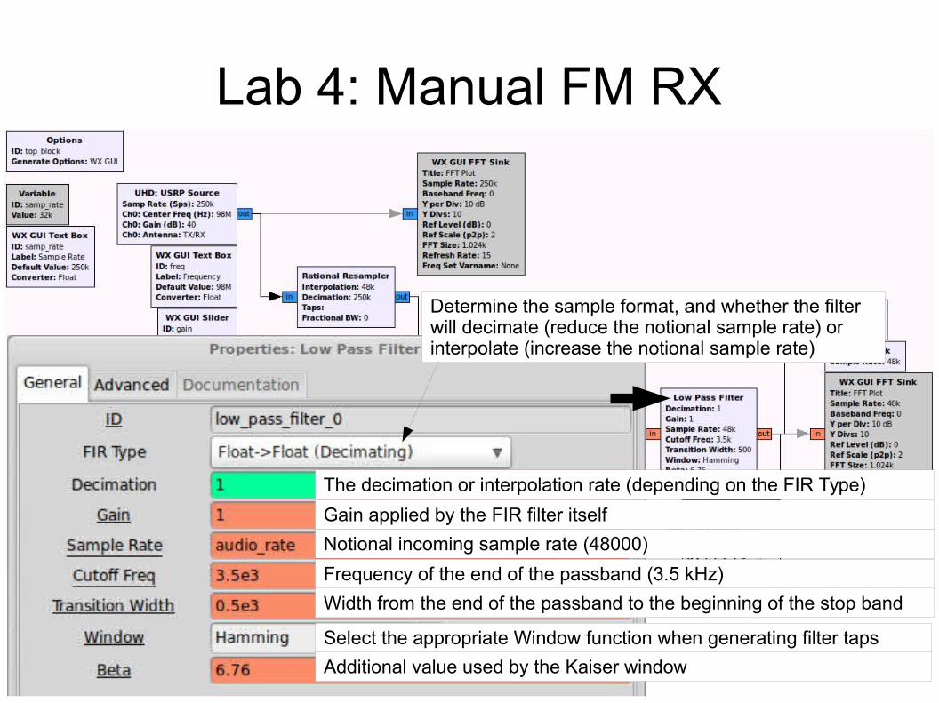
Determine the sample format, and whether the filter will decimate (reduce the notional sample rate) or interpolate (increase the notional sample rate)

The decimation or interpolation rate (depending on the FIR Type)

Gain applied by the FIR filter itself

Notional incoming sample rate (48000)

Frequency of the end of the passband (3.5 kHz)

Width from the end of the passband to the beginning of the stop band

Select the appropriate Window function when generating filter taps

Additional value used by the Kaiser window

Lab 4: Manual FM RX

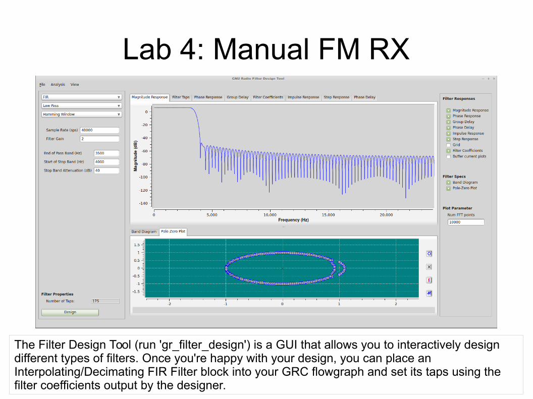
The Filter Design Tool (run 'gr_filter_design') is a GUI that allows you to interactively design different types of filters. Once you're happy with your design, you can place an Interpolating/Decimating FIR Filter block into your GRC flowgraph and set its taps using the filter coefficients output by the designer.

Lab 4: Manual FM RX

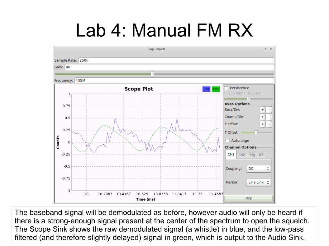
The baseband signal will be demodulated as before, however audio will only be heard if there is a strong-enough signal present at the center of the spectrum to open the squelch. The Scope Sink shows the raw demodulated signal (a whistle) in blue, and the low-pass filtered (and therefore slightly delayed) signal in green, which is output to the Audio Sink.

Lab 5: FM TX

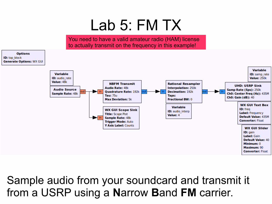
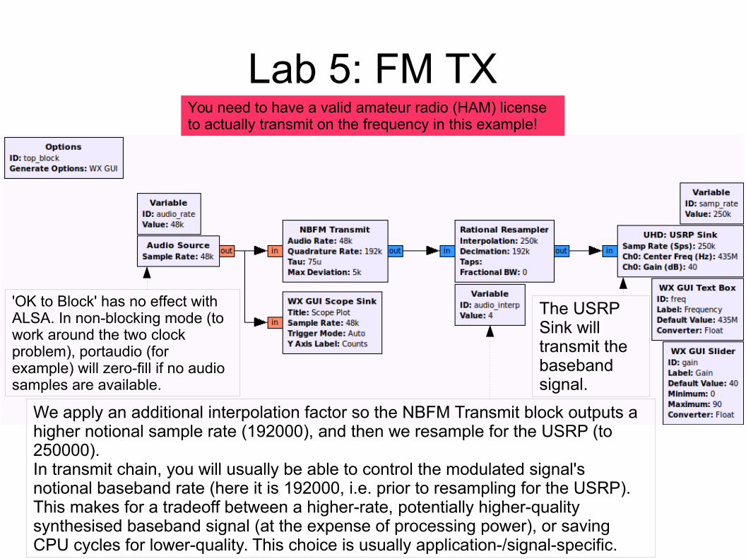
Sample audio from your soundcard and transmit it from a USRP using a Narrow Band FM carrier.

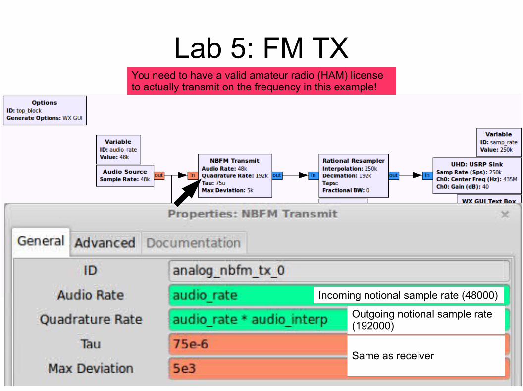
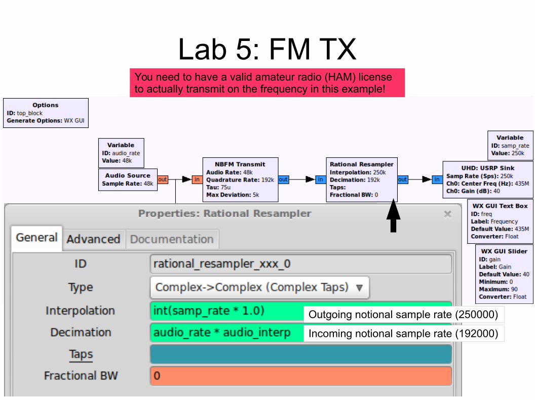
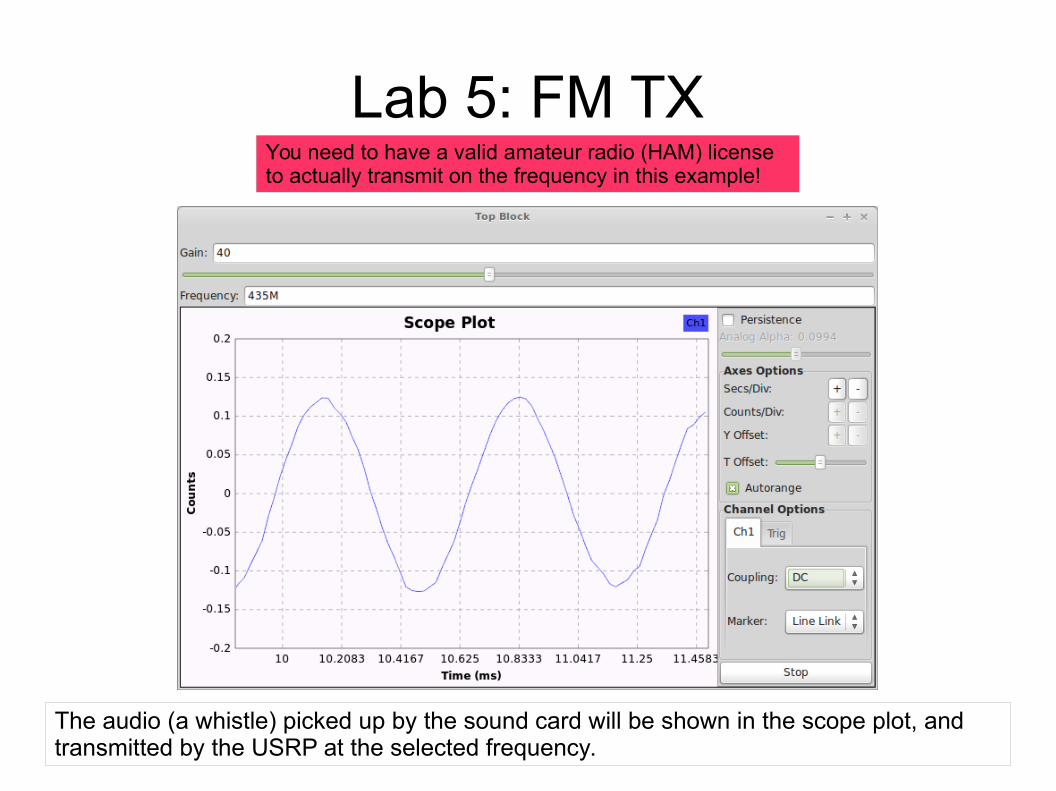
You need to have a valid amateur radio (HAM) license to actually transmit on the frequency in this example!

Lab 5: FM TXYou need to have a valid amateur radio (HAM) license to actually transmit on the frequency in this example!

We apply an additional interpolation factor so the NBFM Transmit block outputs a higher notional sample rate (192000), and then we resample for the USRP (to 250000).In transmit chain, you will usually be able to control the modulated signal's notional baseband rate (here it is 192000, i.e. prior to resampling for the USRP).This makes for a tradeoff between a higher-rate, potentially higher-quality synthesised baseband signal (at the expense of processing power), or saving CPU cycles for lower-quality. This choice is usually application-/signal-specific.

'OK to Block' has no effect with ALSA. In non-blocking mode (to work around the two clock problem), portaudio (for example) will zero-fill if no audio samples are available.

The USRP Sink will transmit the baseband signal.

Lab 5: FM TX

Incoming notional sample rate (48000)

Outgoing notional sample rate (192000)

Same as receiver

You need to have a valid amateur radio (HAM) license to actually transmit on the frequency in this example!

Lab 5: FM TXYou need to have a valid amateur radio (HAM) license to actually transmit on the frequency in this example!

Outgoing notional sample rate (250000)

Incoming notional sample rate (192000)

Lab 5: FM TXYou need to have a valid amateur radio (HAM) license to actually transmit on the frequency in this example!

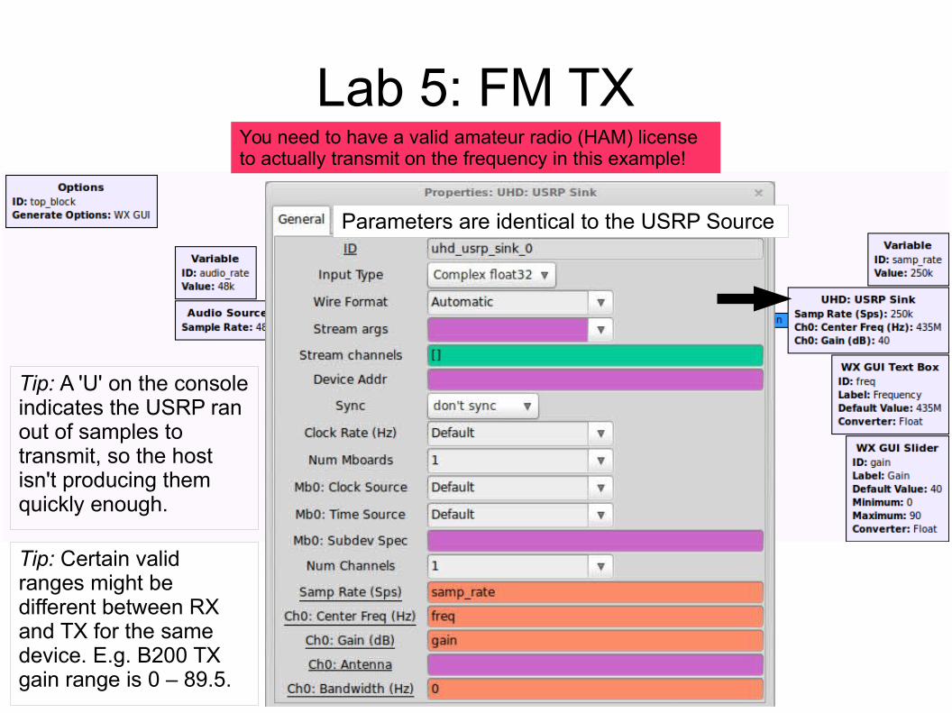
Parameters are identical to the USRP Source

Tip: Certain valid ranges might be different between RX and TX for the same device. E.g. B200 TX gain range is 0 – 89.5.

Tip: A 'U' on the console indicates the USRP ran out of samples to transmit, so the host isn't producing them quickly enough.

Lab 5: FM TX

The audio (a whistle) picked up by the sound card will be shown in the scope plot, and transmitted by the USRP at the selected frequency.

You need to have a valid amateur radio (HAM) license to actually transmit on the frequency in this example!

Lab 5: FM TX

● If you see lots of the letter 'U' in the console, the transmit chain of the USRP is experiencing underruns: samples cannot be produced quickly enough by the host.

● In this example (under Linux/ALSA) it will occur because of the 'two clock' problem, but cannot be fixed by changing 'OK to Block' since the Audio Source is producing samples that are all being consumed without issue, but it happens to be doing this a little too slowly.

Lab 5: FM TX

● It is possible to cheat by adding a 'fudge', or 'twiddle', factor to the Interpolation rate at the Rational Resampler.

● In the example it was:– int(samp_rate * 1.0)

● We can ask the resampler to produce more samples for the same number of input samples so that the USRP will always have enough samples to transmit

● The Interpolation rate would become:– int(samp_rate * 1.01)

– The notional output rate was increased by 1% (1.0 + 0.01),which equals = 252500.The USRP UHD Sink will still consume at 250000.

GNU Radio:

http://gnuradio.org/

CGRAN:

http://cgran.org/

Ettus Research:

http://ettus.com/

UHD Docs:

http://files.ettus.com/uhd_docs/doxymanual/html/