Embed Size (px)
Citation preview

1220
[Journal of Political Economy, 2003, vol. 111, no. 6]� 2003 by The University of Chicago. All rights reserved. 0022-3808/2003/11106-0008$10.00
Gold into Base Metals: Productivity Growth in
the People’s Republic of China during the
Reform Period
Alwyn YoungUniversity of Chicago
With minimal sleight of hand, it is possible to transform the recentgrowth experience of the People’s Republic of China from the ex-traordinary into the mundane. Systematic understatement of inflationby enterprises accounts for 2.5 percent growth per year in the non-agricultural economy during the first two decades of the reform period(1978–98). The usual suspects (i.e., rising participation rates, im-provements in educational attainment, and the transfer of labor outof agriculture) account for most of the remainder. The productivityperformance of the nonagricultural economy during the reform pe-riod is respectable but not outstanding. To the degree that the reformshave improved efficiency, these gains may lie principally in agriculture.
I. Introduction
Between 1978 and 1998, gross domestic product per capita in the Peo-ple’s Republic of China, as reported in official statistics, grew 8.0 percentper year, a performance that makes China the most rapidly growingeconomy in the world during this period, as well as all of recordedhuman history.1 While the unprecedented growth of the Chinese econ-omy can be taken as evidence of the success of its economic reforms,its breathtaking magnitude and inordinate endurance have led others
I am grateful to Robert McCulloch for many useful conversations and to my colleaguesat the Canadian Institute for Advanced Research for helpful feedback. This research wassupported by the Canadian Institute for Advanced Research.
1 All growth rates cited in this paper are ln growth rates; all data, unless otherwise noted,come from the annual issues of the China Statistical Yearbook (CSY).

productivity growth 1221
to seek less favorable, statistical, explanations. Thus Summers and Hes-ton (1994), in version 5.6 of their popular international data set, citethe fact that “it is widely felt that [China’s] growth rates are too high”and, accordingly, arbitrarily lower the reported growth of consumptionand investment during the 1980–93 period by 30 percent and 40 per-cent, respectively. In this paper I take a slightly different approach.Rather than discount the Chinese statistical record, I embrace it. Ac-cepting all the numbers the statisticians of the People’s Republic pro-duce, but making systematic adjustments using their own data, I showthat one can (a) reduce the growth rate during the reform period tolevels previously experienced by other rapidly growing economies, sothat (b) once one takes into account rising labor force participation,the transfer of labor out of agriculture, and improvements in educa-tional attainment, labor and total factor productivity growth in the non-agricultural economy are found to be 2.6 and 1.4 percent per year,respectively; a respectable performance, but by no means extraordinary.
This paper proceeds as follows: Section II begins with a short reviewof the methodology of total factor productivity computations for theuninitiated. Sections III–VII then explain, step by step, how I deriveestimates of output, labor input, human capital, physical capital, andfactor income shares to implement this methodology. In these sectionsI discuss problems with Chinese statistics and the basis on which I havechosen among alternative series. While the estimated growth of pro-ductivity is lowered by some choices (e.g., when I substitute alternativeprice indices, showing higher rates of inflation, for the national accountsdeflators), it is raised by others (e.g., when I substitute a slower-growinglabor series for the official data). In each case, however, I follow theprecept of accepting the Chinese statistical record, making adjustmentsonly when other official series are available, and then only in cases inwhich the deficiencies of the commonly emphasized measures are wellknown or easily recognized. Section VIII brings the different compo-nents together, estimating total factor productivity growth in the non-agricultural economy, and Section IX concludes the paper.
The data of most economies are filled with apparently inconsistentseries. By choosing among them, one can produce almost any estimateof productivity growth imaginable. Consequently, the only value addedin a paper of this sort lies in its treatment and exposition of data,following which the actual total factor productivity results are a mereafterthought. In this paper I depart from standard practice, minimizingthe discussion of productivity methodology and results, and devotingalmost the entire paper to a discussion of Chinese data. To keep thetask manageable, I focus on the reform period (1978–98) alone, es-chewing any temptation to delve into the data of the plan period, whichinvolve a variety of additional issues. I explore the construction and

1222 journal of political economy
biases of each of the alternative data series available for the reformperiod. In the process, I show that the measures of outputs and inputsI select, combined with other data on the Chinese economy, form aninternally consistent whole, with, for example, my measures of laborgrowth matching demographic and participation trends, as well as out-put, wage, and factor share data. Readers can, however, see the steps Itake to reach this conclusion and decide what problems exist in mymethods and what alternatives they would prefer.
This paper restricts its analysis of total factor productivity growth tothe nonagricultural sector. Land is of great importance in agriculture,but any measure of this input faces the formidable problem of its propervaluation relative to the other elements of the economy’s capital stock.Land, however, plays less of a role in the nonagricultural segments ofthe economy.2 In developing economies, much of the investment inagriculture involves livestock and labor-intensive land improvement(e.g., irrigation works). These components are rarely captured in thenational accounts measures of capital investment in machinery and con-struction, which fuel the capital stock estimates of most total factorproductivity studies. Finally, the annual yield of agriculture is heavilyinfluenced by the weather, which has to be controlled for in estimatingproductivity growth. In sum, the study of agriculture, while of greatimportance, involves a host of unique data and estimation problems. Iavoid them by concentrating on the nonagricultural economy alone.
II. Methodology
Let value added be a constant returns to scale function of capital andlabor inputs
Y p F(K, L, t), (1)
where the appearance of t, time, as an independent argument on theright-hand side highlights the fact that the production function evolvesover time. Totally differentiating and dividing by value added, one findsthat
dY F K dK F L dL FK L tp � � dt, (2)( ) ( )Y Y K Y L Y
where represents the partial of F with respect to argument i. WithFi
competitive markets, factors are paid their marginal products, so thatthe terms in parentheses on the right-hand side represent the share of
2 For example, Kim and Park (1985, table 5-13) estimate that land input accounts foronly 4 percent of Korean nonagricultural, nonresidential income during the 1960s and1970s.

productivity growth 1223
each factor in total factor payments. Total factor productivity growth,the last term on the right-hand side, represents the proportional in-crease in output that would have occurred in the absence of any inputchanges and is calculated as a residual item by subtracting the contri-bution of capital and labor from output growth:
dY dK dLTFP growth p � V � VK LY K L
dY dK dY dLp V � � V � , (3)K L( ) ( )Y K Y L
where I have made use of the fact that given constant returns to scale,and , the shares of capital and labor in total factor payments, sumV VK L
to one. As shown by (3), the assumptions of constant returns to scaleand competitive markets provide a formal justification for the ratherintuitive notion of evaluating overall productivity growth as a weightedaverage of the growth of partial productivities, with weights given bythe share of each factor in total income.
Labor and capital inputs are quite differentiated, and variations overtime in the composition of these inputs may play a role in explaininggrowth. To this end, let, for example, overall labor services be a constantreturns to scale function of N types of labor:
L p H(L , L , … , L ). (4)1 2 N
Differentiating, one finds the growth of overall labor services to be aweighted average of the growth of each type of differentiated labor:
dL dLip v , (5)� iL Li i
where . Under the assumption of competitive markets, thev p H L /Hi i i
relative productivities of different types of labor are revealed by(H /H )i j
their relative wages, and equation (5) places greater weight, relative totheir share of the total number of workers, on the growth of types oflabor with higher relative wages.3 The difference between the growthof this weighted aggregate and the growth of the overall labor force,undifferentiated by type, may be taken as the contribution of “humancapital.” Capital input may be similarly disaggregated, although, given
3 Conceptually, H is identified only up to a scalar multiple, since one could double theeffective labor associated with each type of labor input, doubling H and halving themarginal product of labor in F, without meaningfully changing the productive relationshipsin the economy. Equation (4) allows the relative productivities of labor types to differ,which, as highlighted by (5), has implications for the calculation of their contribution togrowth.

1224 journal of political economy
the limitations of Chinese data, I shall not pursue such adjustmentshere.
To implement the preceding methodology, it is necessary to developmeasures of the growth of real value added, labor input (differentiatedby type), and capital input, along with estimates of relative wages andoverall capital and labor income shares. The remainder of the paper isdevoted to these tasks.4
III. Output
China’s national income statistics are, in the main, based on the reportsof local officials, which are passed up through the bureaucracy andaggregated to produce the national figures circulated by the State Sta-tistical Bureau (SSB). Since officials are rewarded for superior perfor-mance and punished for failing to meet targets, it is not surprising thatthey have a tendency to modify their statistical reports in accordancewith central policy objectives, as has been documented, repeatedly, bynone other than the Chinese themselves.5 On the basis of press reports,official opinion appears to be that local officials overstate the growthof output, while understating investment and births.6 In the absence ofa history of independent and comprehensive survey data, there is nosystematic way to evaluate or correct the bias in local reports. It is pos-sible, however, to identify and quantify biases introduced by the statisticalmethods of the SSB. I discuss these biases, and possible corrections, in
4 To apply the continuous-time methodology sketched above to the case of discrete data,I make use of ln growth rates for factor inputs and Tornqvist (average of initial and final)factor income weights. This can be justified, explicitly, by reference to a translog productionfunction (Christensen, Jorgenson, and Lau 1973), which in turn can be taken as a second-order approximation to any given production function.
5 Some fairly frank reporting on the problem of statistical exaggeration, and its foun-dation in the incentives and rewards faced by lower-level officials, can be found in thefollowing sources (as reported and translated by the Foreign Broadcasting InformationService): Changsha Hunan Provincial Service, 1100 GMT, 1 December 1985; Cheng Mingno. 198, 1 April 1994, p. 1; Guangming Ribao, 24 March 1995, p. 1; Hsin Pao, 24 November1993, p. 22; Liaowang, 20 February 1995, p. 1; Renmin Ribao, 18 March 1985, p. 1; 13February 1994, p. 2; 24 June 1994, p. 5; 17 August 1994, p. 1; and 15 December 1999, p.4; Xinhua Domestic Service, 0222 GMT, 13 June 1994; 0513 GMT, 17 January 1995; and1013 GMT, 2 March 1995; and Zhongguo Tongxun She, 1137 GMT, 1 January 1995. Ishould note that the rewards for reporting good performance involve, in some cases,clearly stipulated targets and benefits. Thus, in some localities, township officials “may bepromoted to deputy county level positions so long as the output value of the townshipenterprises exceeds 100 million yuan” (Zhongguo Tongxun She, 1137 GMT, 1 January1995); a State Council decree of 1984 established output targets, varying with populationsize, that would allow counties to be reclassified as cities, thereby automatically entitlingthem to a greater share of enterprise profits and, apparently, higher state subsidies (Chan1994, pp. 273–76). On the flip side, local officials may be punished for failing to meetparticular targets, as reported, e.g., in a Xinhua, 1516 GMT, 5 March 1995, broadcast.
6 See Renmin Ribao, 17 August 1994, p. 1, and 22 April 1995, p. 1, as well as a XinhuaDomestic Service, 2041 GMT, 28 June 1995, broadcast.

productivity growth 1225
TABLE 1Gross Industrial Output and Value Added (100 Million Yuan)
Gross Output
State EnterprisesTownship and
Village
NationalAccounts
Value Added
Original Revised Original Revised Original Revised Original Revised
1990 23,924 23,924 13,064 13,064 4,835 6,858.0 6,858.01991 28,248 26,625 14,955 14,955 5,935 8,087.1 8,087.11992 37,066 34,599 17,824 17,824 8,957 7,166 10,284.5 10,284.51993 52,692 48,402 22,725 22,725 13,950 10,537 14,143.8 14,143.81994 76,909 70,176 26,201 26,201 23,423 17,760 18,358.6 19,359.6
Source.—Original, 1995 CSY; revised, 1996 and later CSY.
this section, examining problems in the measurement of nominal valueadded and the techniques used in its deflation.
A. Nominal Value Added
With regard to the measurement of nominal quantities, the SSB’s re-luctance to revise downward official figures and the approach it hastaken in bringing its statistical system in line with international preceptshave, arguably, imparted an upward bias to the growth of nominal valueadded in the industrial and service sectors.
The SSB appears reluctant to revise national accounts figures sub-stantially downward once they have been released. The most compellingexample of this problem is given by the revision of the gross industrialoutput series, which took place in the mid-1990s. In table 1, I reportthe original gross industrial output series, up to 1994. Following a na-tionwide audit of statistical reports, the 1994 gross industrial outputestimates were revised downward by about 9 percent, with most of theadjustment falling on township and village enterprises, whose outputwas deemed to have been exaggerated by about a third. As shown inthe table, the output series for earlier years was “smoothed” in accor-dance with the new, lower, output estimates.7 In the table I also reportthe national accounts industrial value added series prior to and after
7 Following the 1995 Industrial Census, a new definition of gross output (excludingvalue-added taxes and redefining the gross output measure for outsourced production)was introduced that reduced the gross output estimates further. The revised data for1990–94, which drew on reduced estimates of output, should not be confused with thislater revision, based on new definitions of output. The 1997 CSY clearly indicates that therevised 1990–94 figures (presented in table 1) are based on the old definitions and, infact, links the old and new series by presenting comparable figures for 1995. ZhongguoXinxi Bao (4 May 1995, p. 1; as translated by the Foreign Broadcasting Information Service)also reports that the reduced estimates for 1994 and earlier were the result of the auditingand correction of exaggerated reports.
1226 journal of political economy
the revision of the industrial output series. As the reader can see, thenational accounts industrial value added for 1994 was revised upward,whereas for earlier years it was kept unchanged. Hsueh and Li (1999)provide a comprehensive official description of Chinese statistical meth-ods. They explain that the SSB estimates industrial value added by takingthe gross output series and applying information on the use of inter-mediate inputs gleaned from its more detailed surveys of “independentaccounting” (principally, large and state) enterprises.8 Consequently, a9 percent downward revision in the gross output series, with no changein the estimates for state enterprises, should have led to an equivalentdownward revision of nominal value added. No such revision took place.While the Chinese government has conducted laudable campaignsagainst statistical misrepresentation, recording no less than 70,000 suchcases in 1994 and 60,000 in 1997,9 this information has difficulty infinding its way into revisions of the GDP estimates.
Regarding the service sector, under the Material Planning System,that is, the statistical system used under the plan, only the productionand distribution of material goods were considered a source of outputor income. Thus freight transport, commerce, and even post were con-sidered as output, but items such as passenger transport, real estate,television and radio broadcasting, education, research, finance, insur-ance, and public administration were not. With the exception of a fewlimited areas, such as passenger transport, where detailed statistics werekept through the years, the measurement of most service sectors wasneglected. Consequently, when, during the reform period, the SSBswitched to a System of National Accounts, with its more standard def-inition of output and income, it was ill-equipped to provide a propermeasure of the service sector. Acknowledgment of this defect led to the1991–92 Census of Services, which produced a dramatic revision of thenational accounts.
Table 2 reproduces the SSB’s estimates of the GDP of the service(tertiary) sector, as reported in the CSY. Beginning with the 1995 issueof the publication, the GDP estimates were revised on the basis of thedata from the Census of Services. As the reader can see, the estimatedvalue of service sector output in 1993 was raised by about a third, whereasthe estimates for 1978 were hardly changed at all. In other words, whenthe SSB improved its measurement of the service sector, it concludedthat virtually all the newly discovered, and hitherto unrecorded, value
8 This approach is consistent with that taken, in numerous areas, in other economies(see also Sec. VII below). Typically, aggregate information is limited to a few crude mea-sures, such as gross output, which are then transformed into value-added estimates usingmore detailed surveys of large enterprises.
9 See Zhongguo Tongxun She, 0730 GMT, 23 February 1995; Zhongguo Xinxi Bao, 4May 1995, p. 1; and Beijing Xinhua, 1014 GMT, 25 January 1999.

productivity growth 1227
TABLE 2Nominal GDP of the Service Sector
(100 Million Yuan)
1994 CSY 1995 CSY
1978 824.8 860.51980 918.6 966.41984 1,527.0 1,769.81985 2,119.2 2,556.21986 2,431.0 2,945.61987 2,851.2 3,506.61988 3,656.0 4,510.11989 4,491.6 5,403.21990 4,946.9 5,796.31991 5,797.5 7,227.01992 6,863.4 9,135.91993 8,485.4 11,204.5
added had developed during the reform period. While the developmentof nonmaterial sectors was neglected under the plan, so was their mea-surement. Consequently, the approach adopted by the SSB seems some-what extreme, since it is likely that a fair amount of the newly discoverednonmaterial output was present in 1978. As an alternative, one mightassume that the ratio of unmeasured to measured activity found in 1993existed in 1978 as well. If so, the SSB’s adjustments overstate the growthof service sector nominal output between 1978 and 1993 by 1.6 percentper year.
Despite the problems discussed above, in this paper I defer to theSSB estimates of nominal value added. Any assumption about the quan-tity of unmeasured service sector output in 1978 is equally arbitrary,whereas an adjustment of the entire industrial value added series basedon gross output revisions for the 1990–94 period would be heroic inthe extreme. The growth of industrial and service nominal value addedmay be overstated, but it cannot be credibly adjusted.
B. Deflators
The statisticians of most countries estimate real GDP by deflating nom-inal GDP using separate, independently constructed, price indices. Thisis not the procedure in the People’s Republic. Beginning with the caseof secondary industry (mining, manufacturing, utilities, and construc-tion), in China, enterprises are called on to report the value of outputin current and constant (base year) prices. The difference between thetwo series produces an implicit deflator, which is then used to deflatenominal value added (also reported by the enterprises). Historically,this statistical method dovetailed neatly with the reporting requirementsof the plan and, despite a general movement away from socialist statis-

1228 journal of political economy
tical methods, remains in use today. In regard to the primary sector(farming, fishing, forestry, and animal husbandry), a similar approachis taken, although double deflation of value added is achieved by com-bining the enterprise implicit output deflators10 with separate price in-dices for intermediate inputs. Finally, in regard to the tertiary sector(services), a variety of methods are used, ranging from single deflationusing enterprise-provided implicit output deflators (telecommunica-tions and wholesale and retail trade), to extrapolation using real volumeindices (transport), to single deflation using specialized price indices,some of which are woefully inappropriate (e.g., interest rates in fi-nance!).11 Despite these riders and exceptions, it is fair to say that,overall, the SSB remains heavily dependent on enterprise-provided, out-put-based implicit deflators to deflate nominal value added.12
Ruoen (1995) and Woo (1995) argue that the implicit deflators pro-vided by Chinese enterprises are systematically biased. Enterprises arewell aware of the current value of output and the nominal material valueexpended in its production, and so they can easily report these valuesto statistical officials. However, the construction of accurate constantprice estimates in the base year of the SSB’s choosing is an arduous taskthat, with the relaxation of government control over state enterprisesand the development of nonstate firms during the reform period, isincreasingly unlikely to be seriously undertaken. Ruoen and Woo arguethat many firms assume that the constant price value of output equalsthe nominal value, that is, that the implicit deflator always equals one.This simplifying assumption has been taken by statisticians in other coun-tries (e.g., Singapore [Young 1995, p. 658]), and it seems likely thatChinese firms would find it to be a time-saving approach. More generally,enterprises might assume that the inflation rate has some constant value.
10 As there has been a general privatization of agriculture during the reform period,the SSB uses reports from the remaining state and military farms, supplemented withsurveys of the agricultural sector (Hsueh and Li 1999, p. 94).
11 The use of nominal interest rates to deflate the loan income of banks would measureincreases in the nominal value of loans brought about by inflation as an increase in thereal volume of financial intermediation! While the preceding discussion lays out the formalSSB statement of its procedures (Hsueh and Li 1999), there are indications that, inpractice, these methods are not exactly followed. For example, the value added of whole-sale, retail, and restaurant trade is supposedly deflated using the enterprise implicit outputdeflators (p. 107). However, between 1978 and 1982, the implicit deflator for this sector,in the national accounts, fell 16.6 percent per year! During the same period, the overallGDP deflator rose 2.3 percent per year, and the retail price index rose 3.0 percent peryear. It is impossible to believe that even the most brazen enterprise directors would reporta total collapse of final commercial prices during a period of moderate retail and GDPinflation.
12 The expenditure side of the accounts depends more on independent price indicesbut makes use of a number of grossly incorrect procedures (e.g., using the consumptionbasket of government workers to deflate nominal government expenditure) to balancethe two accounts. Section VI discusses the expenditure accounts in detail.

productivity growth 1229
TABLE 3Average Rates of Inflation (1978–98)
Sector Index Rate of Inflation
Primary sector Implicit deflator 8.5Farm and sideline products pur-
chasing price index7.9
Secondary sector Implicit deflator 4.4Ex-factory industrial price index 6.1Industrial products rural retail
price index5.3
Retail price index 6.6
Tertiary sector Implicit deflator 7.1Consumer price index (services) 10.7
Regardless, the assumption of a constant inflation rate, be it zero orpositive, will make the GDP deflators insufficiently responsive to a surgein the underlying rate of inflation, such as has occurred during thereform period. Fortunately, the SSB does actually compile independentprice indices of its own. It simply does not use them to deflate output!Ruoen (1995) argues that these independent price indices can crediblysubstitute for the existing implicit deflators in the estimation of thegrowth of real output.
Table 3 compares the average rates of inflation recorded by the im-plicit GDP deflators with those of the independent price indices com-piled by the SSB. Beginning with the secondary sector, the ex-factoryindustrial price index, recommended by Ruoen as an alternative to theGDP deflator, covers the factory gate prices of raw materials, electricpower, industrial and construction inputs, and commercial final goods.This index shows 1.7 percent more inflation per year than the implicitsecondary deflator. Alternatives to the ex-factory price index are theindustrial products rural retail price index and the retail price index.Both indices include the profit margins of commercial establishments.In addition, the coverage of the industrial products rural retail priceindex is, obviously, restricted to rural areas, whereas the retail priceindex is basically a consumer goods index. Regressing the growth ofthe implicit secondary deflator on the growth of all three indices, I findthat only the ex-factory index is significant.13 For all these reasons, theex-factory price index is arguably a superior choice as a replacement
13 For the period 1978–98, the coefficients in the regression of the growth of the implicitsecondary deflator on the growth of the industrial products rural price index, the retailprice index, and the ex-factory price index are �.16 (.27), .17 (.25), and .64 (.17), re-spectively (standard errors in parentheses). The industrial products rural price index andthe retail price index are, individually, positively and significantly correlated with thesecondary deflator, but only insofar as they are correlated with the ex-factory price index.

1230 journal of political economy
deflator. It is significant, nevertheless, that during the reform period,all three SSB price indices show more inflation than the implicit sec-ondary deflator. The exaggeration of industrial output growth broughtabout by the use of enterprise deflators has also been independentlyconfirmed by the SSB, which, in a study of Hunan province for theperiod 1982–87, found that a real quantity index, using individual com-modity outputs, implied 3.9 percent less growth per year than indicatedby the implicit deflators (Ruoen 1995, p. 86).
In the primary sector, the long-standing farm and sideline productspurchasing price index, recommended by Ruoen as an alternative tothe primary deflator, measures the average cost of primary-sector goodspurchased by commercial enterprises (of all ownership types), coveringproducts as varied as grains, fruits, vegetables, meat, animal by-products(e.g., furs), fish, and lumber. This index evinces somewhat less inflationthan the implicit GDP deflator, lending no support to Ruoen and Woo’sargument.14 Finally, for the tertiary sector, Ruoen suggests the use ofthe only available service price index, that is, the service price indexsubcomponent of the consumer price index (CPI), which covers postand telecommunications, transport, housing, medical and child care,and other personal and recreational services. The service CPI grew outof the staff and worker cost of living index, which, up until 1985, coveredurban areas alone. In the absence of any alternative, I use the urbanservice price index for 1978–85 and the overall service price index there-after. As shown in the table, the service sector CPI reports the existenceof substantially more inflation than is indicated by the implicit tertiarydeflator.
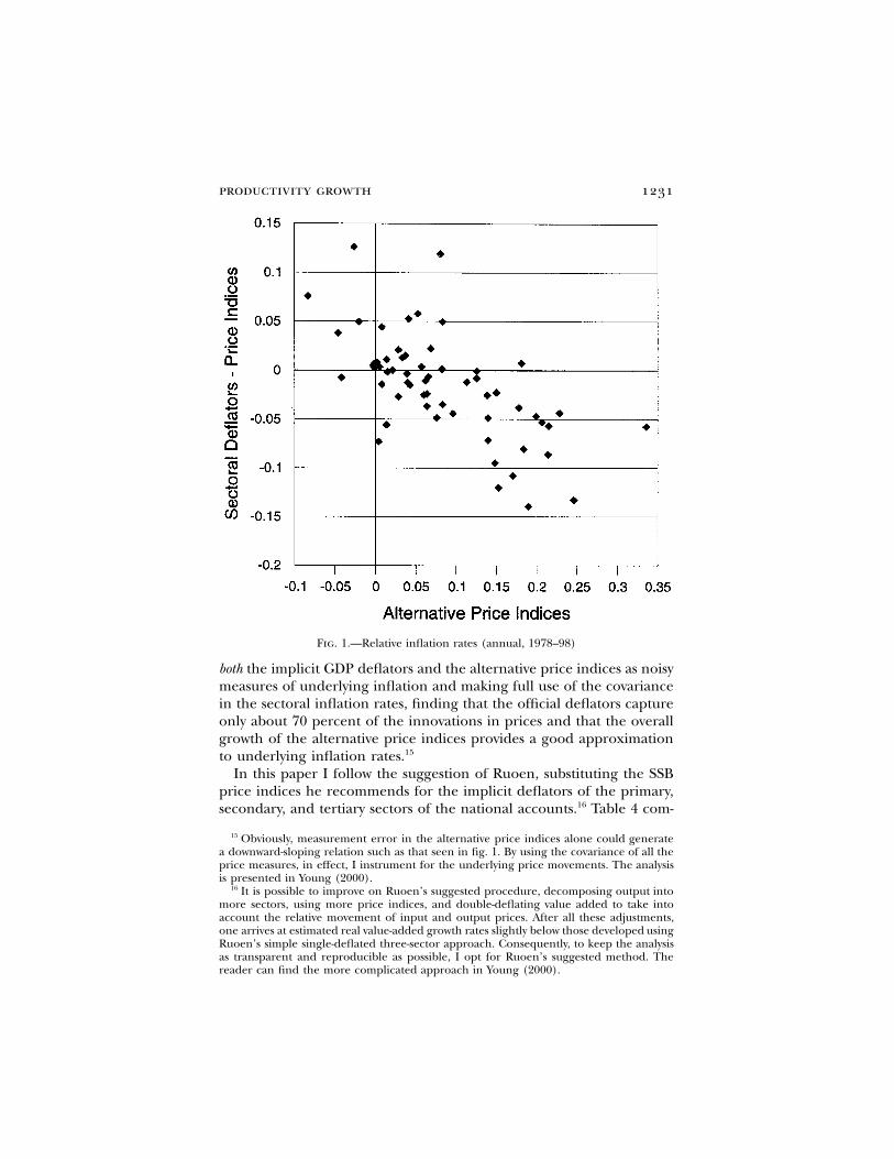
The joint stochastic behavior of the implicit GDP deflators and thealternative price indices collected by the SSB is crudely summarized byfigure 1, which graphs the difference between the growth of each sec-tor’s official deflator and its alternative price index against the inflationpresent in the alternative price index. As the reader can see, the officialdeflators are insufficiently responsive to changes in the underlying in-flation rate as measured by the alternative price indices. In periods ofhigh inflation, the official deflators show smaller price rises (a negativedifference in measured inflation rates), whereas in periods of fallingprices, they evince smaller declines (a positive difference in measuredinflation rates). This is precisely the pattern one would expect if en-terprises economize on effort by assuming price stability or some fixedinflation rate. I have confirmed this result in a formal analysis, treating
14 The reason may be that the implicit deflator is a double-deflated value-added priceindex. With the prices of agricultural goods rising relative to industrial intermediate inputs,the value-added deflator will rise faster than the output deflator. Consequently, it is stillpossible that the agricultural enterprise output deflator grows less than the farm productsprice index.
productivity growth 1231
Fig. 1.—Relative inflation rates (annual, 1978–98)
both the implicit GDP deflators and the alternative price indices as noisymeasures of underlying inflation and making full use of the covariancein the sectoral inflation rates, finding that the official deflators captureonly about 70 percent of the innovations in prices and that the overallgrowth of the alternative price indices provides a good approximationto underlying inflation rates.15
In this paper I follow the suggestion of Ruoen, substituting the SSBprice indices he recommends for the implicit deflators of the primary,secondary, and tertiary sectors of the national accounts.16 Table 4 com-
15 Obviously, measurement error in the alternative price indices alone could generatea downward-sloping relation such as that seen in fig. 1. By using the covariance of all theprice measures, in effect, I instrument for the underlying price movements. The analysisis presented in Young (2000).
16 It is possible to improve on Ruoen’s suggested procedure, decomposing output intomore sectors, using more price indices, and double-deflating value added to take intoaccount the relative movement of input and output prices. After all these adjustments,one arrives at estimated real value-added growth rates slightly below those developed usingRuoen’s simple single-deflated three-sector approach. Consequently, to keep the analysisas transparent and reproducible as possible, I opt for Ruoen’s suggested method. Thereader can find the more complicated approach in Young (2000).

1232 journal of political economy
TABLE 4Estimated Growth of Real GDP (1978–98)
Aggregate Nonagricultural
Official .091 .106Alternative .074 .081
pares the official Chinese growth rates with the alternative estimates ofGDP growth.17 As the table shows, the use of the alternative SSB priceindices to deflate output lowers the growth of aggregate and nonagri-cultural GDP by 1.7 percent and 2.5 percent, respectively. These ad-justments are substantially less than those made by Summers and Hestonversion 5.6, which, for the period 1978–92, when official GDP grew 8.9percent per year, reports an adjusted aggregate GDP growth rate of 5.6percent.18 Figure 2 graphs the official and price index–adjusted annualgrowth of GDP achieved since 1978. All of the downward adjustmentin the growth rate brought about by the deflator substitution comesafter 1986, with growth from 1986 to 1998 averaging 6.2 percent peryear, 3 percent less than the officially reported figure of 9.2 percent. In1989, a year of economic retrenchment, GDP is now seen to have fallenby 5.2 percent, as opposed to the 4.0 percent positive growth reportedin official figures. This provides some insight into the forces that pre-cipitated the political unrest of that year.
IV. Labor
In the People’s Republic there are two sources of data on the total andworking population: the annual administrative and survey-based esti-mates reported in the CSY and the tabulations of the occasional pop-ulation censuses. In table 5, I compare the figures found in the twosources. As the reader can see, the annual population estimates arequite close to those reported by the censuses. This is not surprising sincethe former, although based on residence registration and sample sur-
17 Official Chinese growth rates are computed using Laspeyres price weights. I computeaggregate growth rates as the Tornqvist weighted sum of the sectoral growth rates, i.e.,
s (t) � s (t � 1)i ig(t) p g (t) ,� i [ ]2i
where is the share of sector i in the nominal value added of year t, and is thes (t) g (t)i i
constant price growth of the output of sector i between years and t. In reportingt � 1“official” growth rates in the table, I reestimate the official growth rate using this procedure,which lowers the official growth rate by 0.2 percent per year.
18 For the same period, my adjustments lower the growth of aggregate GDP to 7.7 percentper year.

productivity growth 1233
Fig. 2.—GDP growth during the reform period
TABLE 5Chinese Population and Labor force Data (Millions)
China Statistical Yearbook
Employment Census Sources
Population Old Series Revised PopulationWorking
Population
1978 963 402 4021982 1,017 453 453 1,008 5221989 1,127 553 5531990 1,143 567 639 1,134 6471997 1,236 637 6961998 1,248 624 700Growth:
1982–90 1.5 2.8 4.3 1.5 2.71978–98 1.3 2.2 2.8
Note.—Total population numbers include the military, whereas the working population figures do not. Old seriesemployment data for 1997–98 are based on author’s calculations.
veys, are adjusted in accordance with the results of the latter.19 In regardto employment, however, there are large discrepancies both betweenthe census and the annual estimates and, within the annual estimatesthemselves, between the old series and its recent revision. These dis-crepancies require some explanation.
Under the plan, the SSB, using departmental reports and surveys,
19 See the 1999 CSY, p. 110. I should note that the census population figures I reportin the table do not agree with the numbers reported in popular sources (e.g., the CSY)since I have adjusted the census population numbers to agree with the definition usedin the annual series, i.e., adding in the members of the People’s Liberation Army. Thedata presented in this section and the next, in addition to the CSY, draw on the 1982 and1990 population censuses (People’s Republic of China 1982, 1993), the 1987 and 19951% Population Sample Surveys (People’s Republic of China 1988, 1995), and the annualissues of the China Population Statistics Yearbook.

1234 journal of political economy
collected data on the “labor force of society,” which forms the basis forthe “old” CSY series reported in the table. Referring to the workingpopulation, this series had a fairly stringent definition of employment,requiring, for example, that young people in cities and towns with tem-porary employment20 earn, as a minimum, the wage level of local grade1 workers in order to be included in the series (see Chen and Niu 1989,p. 203; Hsueh, Li, and Liu 1993, p. 565). In contrast, the census defi-nition of employment includes all those earning wage or managementincome, whether through permanent or temporary employment.21 Notsurprisingly, the census numbers tend to be greater. In 1997 the em-ployment series reported in the CSY was revised on the basis of theresults of the annual Survey of Population Change. While the figuresfor earlier years were retained, the numbers from 1990 on rose sub-stantially. As the reader can see, on the basis of the similarity of theestimates, the employment definition used by the population surveyappears to correspond more closely with that used in the census.22 Thelinking of the old data on the labor force of society (prior to 1990) withthe new labor force series (from 1990 on) in current official publicationsis regrettable, since it generates spurious labor force growth, which,unfortunately, has been used by some economists as a measure of em-ployment growth. While the labor force of society is no longer reportedas the official aggregate employment series, these data continue to becollected and can be inferred from the detailed tabulations of the CSY.23
I use these data to extend the “old” series to 1998, as reported in table5. However, I am not able to avoid a further discontinuity, introducedin 1998, when the definition of workers in urban enterprises was revised
20 That is, while waiting to exercise their “right” to employment, participation in themilitary, or further schooling.
21 Both censuses required those with temporary employment to work 16 or more daysin the month before the enumeration (1982 census, pp. 606–7; 1990 census, 4:515) andrestricted the working population to those aged 15 and above.
22 The China Population Statistics Yearbook reports the population survey results but givesno detail as to the underlying definitions. In any case, although the revised annual laborforce series represent an adjustment “in accordance with the data obtained from thesample surveys on population changes” (China Statistical Yearbook 1999, p. 133), they arenot literally the population survey results, since the survey indicates even more workingpersons than are reported in the CSY (compare China Population Statistics Yearbook [1998,p. 72] and China Statistical Yearbook [1999, p. 133]). I should also note that much of therevised industry and enterprise (e.g., state vs. collective) details reported in the early 1990sappear to be based on simple “fudge factors”; i.e., if the revised series indicated 9 percentadditional aggregate employment, then the revised estimates of employment by industryor enterprise were increased, similarly, by 9 percent. As its name implies, the originalemphasis of the Survey of Population Change concerned demographics, not the detailsof employment.
23 While the summary tabulations on industry and enterprise employment in the CSYare adjusted to reflect the revised totals, the tables on the detailed industry structure ofemployment continue to be based on the old series, which, consequently, can be extendedby summing the relevant categories.

productivity growth 1235
TABLE 6Participation Rates by Age and Sex
1982 Census 1990 Census 1997 Survey
Male Female Male Female Male Female
Overall .57 .47 .61 .53 .62 .5615–19 .71 .78 .62 .68 .44 .4720–24 .96 .90 .93 .90 .92 .8925–29 .99 .89 .98 .91 .97 .9130–34 .99 .89 .99 .91 .98 .9235–39 .99 .88 .99 .91 .98 .9240–44 .99 .83 .99 .88 .98 .9145–49 .97 .71 .98 .81 .97 .8550–54 .91 .51 .93 .62 .93 .7255–59 .83 .33 .84 .45 .82 .5360–64 .64 .17 .63 .27 .62 .37≥65 .30 .05 .33 .08 .34 .16
Note.—The 1982 and 1990 censuses exclude military personnel from the numerator and denominator. The 1997data do not specify.
to include only those actually working and receiving income (as opposedto those who retained employment contracts, without actually workingin the unit). This resulted in a substantial reduction in the estimatedworking population, particularly in manufacturing.
As table 5 indicates, all sources show labor force growth substantiallyexceeding the growth of the population. To explore the basis of thisresult, in table 6 I report the participation rates by age group and seximplied by census and survey data.24 Between 1982 and 1990, accordingto the census, participation rates for the youngest age groups fell, andthose for middle-aged and elderly women rose slightly. The data of the1997 Population Change Survey extend these trends. These develop-ments are consistent with growing investment in education and thegradual aging of Communist-era women, who are likely to have had agreater history of lifetime market labor force participation than theirpredecessors. They are, however, largely offsetting. Of the increase inthe overall participation rate from .52 to .57 between the censuses of1982 and 1990, only 1.1 percent is due to changes in the age-specificparticipation rates, with fully 98.9 percent attributable to the evolvingage distribution of the population.
Since demographic trends play such an important role in explainingthe rise in participation rates, it is important to examine them in greaterdetail. Table 7 reports the distribution of the population of each sex by
24 Prior to the 1982 census, only fragmentary data on the characteristics of the workforcein particular sectors are available (e.g., Chen 1967, p. 484). The labor force of societyseries, in particular, did not collect information on the characteristics of workers. Con-sequently, it is not possible to estimate labor force participation rates by age group priorto 1982.
1236 journal of political economy
TABLE 7Demographic Trends
Distribution by Age GroupSurviving/Original
Members
1982 Census 1990 Census 1997 Survey 1990/1982 1997/1990
Male Female Male Female Male Female Male Female Male Female
0–4 .10 .09 .10 .10 .07 .06 1.03 1.03 1.09 1.105–9 .11 .11 .09 .09 .10 .09 .99 .99 1.02 1.0110–14 .13 .13 .09 .09 .09 .09 .97 .98 .84 .8515–19 .12 .13 .11 .11 .08 .07 1.01 .99 .89 .9520–24 .07 .07 .11 .11 .08 .08 1.03 .99 .98 1.0225–29 .09 .09 .09 .09 .10 .11 .98 .98 1.02 1.0530–34 .07 .07 .08 .07 .10 .10 .99 .99 .99 1.0335–39 .06 .05 .08 .08 .06 .06 .97 .98 1.01 1.0540–44 .05 .05 .06 .06 .08 .08 .96 .97 1.03 1.0845–49 .05 .05 .04 .04 .06 .06 .93 .95 1.00 1.0850–54 .04 .04 .04 .04 .05 .05 .90 .93 .99 1.0855–59 .03 .03 .04 .04 .04 .04 .83 .88 .95 1.0360–64 .03 .03 .03 .03 .04 .04 .74 .81 .89 .95≥65 .04 .06 .05 .06 .07 .08 .47 .54 .61 .67
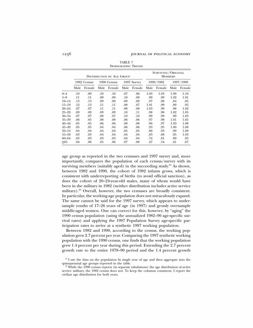
age group as reported in the two censuses and 1997 survey and, moreimportantly, compares the population of each census/survey with itssurviving members (suitably aged) in the succeeding study.25 As shown,between 1982 and 1990, the cohort of 1982 infants grows, which isconsistent with underreporting of births (to avoid official sanction), asdoes the cohort of 20–24-year-old males, many of whom would havebeen in the military in 1982 (neither distribution includes active servicemilitary).26 Overall, however, the two censuses are broadly consistent.In particular, the working-age population does not miraculously expand.The same cannot be said for the 1997 survey, which appears to under-sample youths of 17–26 years of age (in 1997) and grossly oversamplemiddle-aged women. One can correct for this, however, by “aging” the1990 census population (using the annualized 1982–90 age-specific sur-vival rates) and applying the 1997 Population Survey age-specific par-ticipation rates to arrive at a synthetic 1997 working population.
Between 1982 and 1990, according to the census, the working pop-ulation grew 2.7 percent per year. Comparing the 1997 synthetic workingpopulation with the 1990 census, one finds that the working populationgrew 1.4 percent per year during this period. Extending the 2.7 percentgrowth rate to the entire 1978–90 period and the 1.4 percent growth
25 I use the data on the population by single year of age and then aggregate into thequinquennial age groups reported in the table.
26 While the 1990 census reports (in separate tabulations) the age distribution of activeservice military, the 1982 census does not. To keep the columns consistent, I report thecivilian age distribution for both years.

productivity growth 1237
TABLE 8Distribution of the Working Population by Economic Sector
Labor Force of Society Population Census
Agricultural Nonagricultural Agricultural Nonagricultural
1978 .71 .291982 .68 .32 .73 .271990 .60 .40 .72 .281998 .53 .47Absolute growth:
1982–90 1.3 5.6 2.5 3.31978–98 .8 4.5
to the 1990–98 period, one derives an average estimated working pop-ulation growth of 2.2 percent between 1978 and 1998. As can be seenfrom table 5 above, this agrees exactly with the growth reported by the“old” labor force of society employment series (particularly after it re-moved, in 1998, absent workers). In sum, a working population growthof 2.2 percent per year, in excess of the 1.3 percent rate of populationgrowth, is completely consistent with reasonable participation and dem-ographic trends and may be deemed fairly accurate.
To complete this section, I need to derive estimates of the growth ofthe working population in the nonagricultural sector alone. Table 8summarizes the distribution of the working population by economicsector, as reported in the labor force of society data and the census.The labor force of society data indicate a substantial movement of laborout of agriculture into the industrial and service sectors of the economy.In contrast, the census data show an extraordinary stability in sectoralshares. Given the well-known explosion of rural industrial activity duringthe reform period, these data strain credulity. The shift of labor out ofagriculture into the industrial sector is confirmed by the industrial cen-suses of 1985 and 1995, which, as shown in table 9, indicate industriallabor force growth that exceeds that reported in the data of the laborforce of society.
The Chinese population censuses are unusual in that rather than askthe respondents to specify their area of industrial activity, they ask themto provide the name of their place of work, which is then used to de-termine the industrial sector. Thus the 1982 census contains detailedinstructions for enumerators on how the enterprise name should berecorded, even requiring, in the case of large enterprises, a precisespecification of the department name. The 1990 census provides similarinstructions but, perhaps frustrated by the large number of respondentsreporting “agriculture” in the earlier census, emphasizes that peasantsmust report the name of their enterprise (but, still, not its industrialsector). In any case, the instructions then completely undermine the

1238 journal of political economy
TABLE 9Industrial Employment (Millions)
Labor Force of Society Population Census Industrial Census
1982 72 721985 83 941990 97 871995 110 147Absolute growth:
1982–90 3.7 2.41985–95 2.8 4.5
Note.—Industrial refers to mining, manufacturing, and utilities, i.e. the secondary sector other than construction.
accuracy of the statistics by noting that for households that contractland and operate as an independent economic unit, all working mem-bers of the household should report the main household product asthe enterprise name. The confusion created by the use of a single ques-tion to collect two pieces of information, industry of employment anda record, with associated personal names, of each individual’s place ofwork, is obvious.27 In contrast with the census, the labor force of society,since it is based partly on enterprise reports, is much better equipped,albeit not perfectly so, to track the movement of labor between sectors.28
One can make use of a national income identity to verify the accuracyof the intersectoral transfer of labor reported in the labor force of societydata series. The share of labor in nonagricultural GDP equals the sumof worker wages divided by total value added:
� w L � w si i i ii iv p p L , (6)L NANA Q QNA NA
where the index i denotes the various subsectors of nonagricultural GDPand their corresponding shares of total nonagricultural labor. Fromsi
this, it follows that the growth of nonagricultural labor should equalthe (ln) growth of nominal nonagricultural GDP, minus the growth ofweighted wages, plus the growth of the share of labor. Table 10 presentsthe relevant data. Between 1978 and 1998, nominal nonagricultural GDPgrew 16.1 percent per year. Weighting the official series on the wagesof staff and workers by detailed sector using the detailed employmentdistributions of the labor force of society data, I find that weightednominal nonagricultural wages grew 12.5 percent per year. Finally, aswill be seen in Section VII, the national accounts show the income share
27 The statistical purpose served by collecting workplace names is mystifying since thisinformation cannot be meaningfully aggregated.
28 I should note that the broader census definition of employment cannot explain thedifference between the two series. As shown in table 9, the census actually reports lowerabsolute industrial employment in 1990, despite the fact that its overall employmentestimate substantially exceeds that reported in the labor force of society series (table 5).

productivity growth 1239
TABLE 10Consistency between National Income,
Wage, and Employment Data(Nonagricultural Growth Rates, 1978–98)
Nominal GDP 16.1Weighted wages 12.5Share of labor 1.4Implied employment growth 5.0Reported employment growth 4.5
of nonagricultural labor rising 1.4 percent per year. Together, these dataimply a 5.0 percent annual growth in nonagricultural employment. Thelabor force of society indicates growth of 4.5 percent per year. Thus, ifanything, this series may understate the growth of nonagriculturalemployment.29
In this paper I use the data series on the labor force of society tomeasure the growth of labor input. As shown above, the overall growthof the working population in this series is perfectly consistent with rea-sonable demographic and participation data, whereas its nonagricul-tural component, by the standards of the industrial surveys and nationalincome and wage data, is modestly conservative.
V. Human Capital
As noted earlier, a proper measure of the growth of labor input shouldaccount for differentiation in the human capital of the workforce. Whilethe labor force of society data series provides a reasonable measure ofthe overall growth of the labor force and its sectoral distribution, it doesnot contain any information on the characteristics of workers. To adjustfor the changing characteristics of workers, one must turn to censusand occasional survey data. Table 11 summarizes the sex, educational,and age characteristics of the working population, as indicated by the1982 and 1990 censuses, the 1987 and 1995 1% Sample PopulationSurveys, and the 1997 Survey on Population Change. As the table shows,the various censuses and surveys indicate a gradual rise in the proportionof female workers, aging of the labor force, and improvement in itseducational attainment. In the pages that follow, I examine the accuracyof these trends. To shorten the discussion, I focus on the changes from1982 to 1990 (census to census) and 1990 to 1995 (census to survey),
29 Alternatively, one can interpret the data in table 10 as indicating that the growth ofnominal output is overstated by about 0.5 percent per year.

1240 journal of political economy
TABLE 11Distribution of the Working Population by Sex, Education,
and Age Characteristics
1982 1987 1990 1995 1997
A. Sex
Male .563 .555 .550 .543 .535Female .437 .445 .450 .457 .465
B. Educational Attainment
None .282 .229 .169 .126 .116Primary .344 .363 .378 .372 .348Secondary .366 .396 .434 .473 .501Tertiary .009 .012 .019 .029 .035
C. Age Group
!20 .178 .140 .120 .070 .05720–24 .133 .191 .177 .138 .12025–29 .167 .119 .152 .168 .16730–34 .132 .144 .123 .147 .16435–39 .098 .114 .127 .116 .10340–44 .085 .083 .092 .123 .12445–49 .077 .069 .068 .088 .09550–54 .057 .059 .055 .060 .06555–59 .038 .041 .042 .044 .04560–64 .021 .023 .024 .027 .031≥65 .015 .017 .019 .020 .029
since I shall use these two discrete growth periods to measure the growthof human capital during the reform period.30
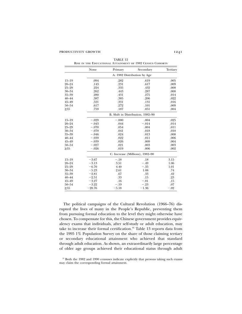
The preceding section established the reasonableness of the demo-graphic and employment trends by sex and age present in the Chinesecensus data. I now turn to the educational data. Table 12 reports thedistribution of educational attainment by age cohort in the aggregateChinese population as recorded in the 1982 census. The table thensubtracts this distribution from that present in the (suitably aged) equiv-alent cohort in the 1990 census. While a rise in the educational attain-ment of young cohorts, who would still be pursuing formal schooling,is to be expected, in the Chinese data, improvements in educationalattainment extend deeply into older age groups. Better-educated per-sons are likely to have lower mortality rates (which will shift the edu-cational distribution up as cohorts age), but, as panel C of the tableshows, this does not explain the Chinese data, where the absolute num-ber of educated persons in older age cohorts rises from one census tothe other!
30 I do not have access to data on the educational attainment of the total populationfor the 1997 survey. As I need this information to generate a synthetic educational at-tainment (see below), I rely on the 1995 survey instead.
productivity growth 1241
TABLE 12Rise in the Educational Attainment of 1982 Census Cohorts
None Primary Secondary Tertiary
A. 1982 Distribution by Age
15–19 .094 .282 .619 .00520–24 .143 .231 .617 .00925–29 .224 .335 .432 .00830–34 .262 .443 .287 .00835–39 .280 .431 .275 .01440–44 .387 .385 .206 .02245–49 .521 .331 .131 .01650–54 .617 .272 .101 .009≥55 .759 .187 .051 .004
B. Shift in Distribution, 1982–90
15–19 �.029 �.000 .004 .02520–24 �.043 .044 �.014 .01425–29 �.070 .054 .004 .01130–34 �.070 .041 .018 .01035–39 �.046 .024 .013 .00840–44 �.039 .022 .011 .00645–49 �.039 .026 .009 .00450–54 �.027 .021 .003 .003≥55 �.026 .019 .006 .002
C. Increase (Millions), 1982–90
15–19 �3.67 �.18 .18 3.1520–24 �3.13 3.51 �.49 1.0625–29 �6.70 4.40 �.35 1.0130–34 �5.23 2.61 1.08 .7435–39 �2.81 .67 .33 .4240–44 �2.51 .33 .15 .2345–49 �3.27 .16 �.01 .1550–54 �3.22 �.19 �.23 .07≥55 �28.76 �5.18 �1.36 �.02
The political campaigns of the Cultural Revolution (1966–76) dis-rupted the lives of many in the People’s Republic, preventing themfrom pursuing formal education to the level they might otherwise havechosen. To compensate for this, the Chinese government provides equiv-alency exams that individuals, after self-study or adult education, maytake to increase their formal certification.31 Table 13 reports data fromthe 1995 1% Population Survey on the share of those claiming tertiaryor secondary educational attainment who achieved that standardthrough adult education. As shown, an extraordinarily large percentageof older age groups achieved their educational status through adult
31 Both the 1982 and 1990 censuses indicate explicitly that persons taking such examsmay claim the corresponding formal attainment.

1242 journal of political economy
TABLE 13Proportion of Individuals Reporting Tertiary and SecondaryEducation Attained through Adult Education (1995 Survey)
Tertiary Upper Secondary
Male Female Male Female
15–19 .22 .23 .04 .0520–24 .29 .35 .07 .0825–29 .36 .40 .08 .0830–34 .47 .52 .07 .0735–39 .58 .59 .07 .0840–44 .59 .55 .12 .1445–49 .52 .46 .14 .1250–54 .32 .23 .12 .0855–59 .22 .14 .11 .0760–64 .22 .14 .11 .08≥65 .17 .09 .09 .06
TABLE 14Mainstream and Adult Education (1998)
Mainstream Adult
Students GraduatesFull-TimeTeachers Students Graduates
Full-TimeTeachers
Primary 139,538 21,174 5,819 5,386 5,485 64Secondary 73,407 21,241 4,312 66,760 88,530 342
Peasant technicaltraining 59,830 82,019 140
Tertiary 3,409 830 407 2,822 826 97
Source.—CSY 1999, tables 20-1, 20-21.Note.—Numbers are thousands of persons.
education courses.32 Data on the annual flow of students in mainstreamand adult education schools (table 14) confirm the relative importanceof continuing education. These data also show, however, the inferiorquality of adult education programs, since they tend to be shorter, witha high ratio of graduates to students, and have much higher student-teacher ratios. While not all such graduates could claim mainstreamequivalency, the mixing of mainstream and adult education in the censusdata on improving educational attainment is clearly problematic, sincethe two types of certification would, most likely, command differentmarket prices. To alleviate any concerns on this dimension, in the anal-ysis below I develop a synthetic 1990 labor force, in which any improve-
32 Not surprisingly, younger age groups also avail themselves of the opportunity to achievehigher levels of certification through this channel.

productivity growth 1243
TABLE 15Consistency between 1990 Census and 1995 Sample Survey
Growth of 1990Cohort Size
Shift in Educational Distributionby Age Cohort
Male Female None Primary Secondary Tertiary
0–4 1.13 1.135–9 1.09 1.0910–14 .94 .9415–19 .86 .93 �.010 �.046 .025 .03120–24 .95 1.03 �.012 �.001 .006 .00725–29 1.01 1.07 �.014 .018 �.012 .00830–34 1.00 1.05 �.019 .012 �.002 .00935–39 1.04 1.08 �.022 .014 .000 .00740–44 1.05 1.10 �.017 .017 �.006 .00645–49 1.04 1.10 �.013 .015 �.007 .00550–54 1.02 1.07 �.015 .012 �.003 .00655–59 1.00 1.06 �.007 .008 �.006 .00560–64 .96 1.03 �.022* .016 .003 .003≥65 .75 .80
Note.—Growth of cohort size includes military personnel in both population estimates. Shift in educational distri-bution does not include military personnel in 1990 figures.
* The numbers in this panel refer to those aged ≥60.
ment in the educational distribution of cohorts aged over 25 in 1982is disallowed.33
I turn next to the 1995 1% Sample Population Survey. Table 15 agesthe quinquennial age cohorts of the 1990 census and compares theresulting distribution to the population recorded by the 1995 survey.Once again, the cohort of 1990 infants expands, reflecting the under-reporting of births. More worrisome, however, is the underreporting ofyouths and oversampling of middle-aged men and, particularly, women,patterns that, as discussed in the preceding section, appear in the 1997Population Survey as well.34 To correct for changes in the samplingdistribution, in the analysis below I construct a synthetic 1995 workingpopulation by aging the 1990 age cohorts (using the 1982–90 annualsurvival rates) and then applying the age#sex labor force participationrates recorded by the 1995 Sample Survey. A comparison of the cohort-specific distribution of educational attainment indicates, as was the casein the 1982–90 period, a systematic rise in the educational attainmentof older cohorts (table 15). Again, to allay concerns on this dimension,I construct an alternative synthetic estimate in which I disallow all im-provements in the educational attainment of cohorts aged over 25 in1990.
33 I allow younger cohorts to improve their attainment, since they could still have beenpursuing formal schooling between 1982 and 1990.
34 This appears to be a characteristic of the 1990s surveys. The 1987 survey, in contrast,is quite consistent with the age distribution of the 1982 and 1990 censuses.

1244 journal of political economy
TABLE 16Measures of Worker Characteristics: Distribution of Working Population
Baseline* Alternative†
1982 1990 1995 1990 1995
A. Sex
Male .563 .550 .552 .550 .552Female .437 .450 .448 .450 .448
B. Educational Attainment
None .282 .169 .119 .195 .152Primary .344 .378 .369 .361 .346Secondary .366 .434 .483 .429 .481Tertiary .009 .019 .029 .015 .021
C. Age Group
!20 .178 .120 .075 .120 .07520–24 .133 .177 .157 .177 .15725–29 .167 .152 .174 .152 .17430–34 .132 .123 .142 .123 .14235–39 .098 .127 .115 .127 .11540–44 .085 .092 .117 .092 .11745–49 .077 .068 .082 .068 .08250–54 .057 .055 .056 .055 .05655–59 .038 .042 .041 .042 .04160–64 .021 .024 .024 .024 .025≥65 .015 .019 .017 .019 .017
* The baseline measures for 1982 and 1990 come from census data; that for 1995 comes from aging 1990 censuspopulation cohorts and applying 1995 educational distribution and sex#age#education participation rates.
† The alternative measure for 1990 comes from aging 1982 census cohorts, retaining 1982 educationaldistribution,and applying 1990 sex#age#education participation rates. The alternative measure for 1995 comes from agingthe alternative 1990 cohorts, retaining alternative 1990 educational characteristics, and applying 1995 sex#age#education participation rates.
Table 16 summarizes my measures of the sex, age, and educationalcomposition of the workforce. The baseline measure accepts the 1982and 1990 census data and estimates the age distribution of the 1995population by aging the 1990 census population using the annualized1982–90 survival rates, using the 1995 survey to determine the partici-pation rates and educational characteristics of each quinquennial agecohort. The alternative measure disallows any improvement in the ed-ucational attainment of cohorts aged over 25 between 1982 and 1990but uses the age#sex#education participation rates of the 1990 censusto determine the labor force participation of the resulting educationallydemoted population. The alternative 1990 population is then aged fur-ther from 1990 to 1995, disallowing any improvements in the educa-tional attainment of cohorts aged over 25 in 1990, and uses theage#sex#education participation rates of the 1995 survey to determinelabor force participation of each group in that year. The resulting mar-ginal distributions are summarized in the table.
Published data on the relative labor incomes of Chinese workers by

productivity growth 1245
worker characteristic are, basically, nonexistent. However, the SSB’s Ur-ban Household Survey has a history of asking for the characteristics andindividual labor income of the members of the survey households. Ihave been able to acquire the survey files for the years 1986–92. I sup-plement them with the files of the Household Survey (urban and rural)executed in 1988 and 1995 by the Chinese Academy of Social Sciences,which contain similar data. (These data can be purchased from theUniversities Service Centre, Chinese University of Hong Kong.) Whilethe surveys cover a large number of provinces and cities, they are byno means a balanced sample (e.g., some provinces are not represented,and the samples, both rural and urban, are heavily biased toward better-educated households). The survey responses also have substantial cod-ing errors and internal inconsistencies, with, for example, non–labormarket participants reporting positive earnings. I narrow the samplesconsiderably by requiring that the respondents consistently, across avariety of questions, identify themselves as working employees in thenonagricultural sector. The final sample size is 222,281 observations. Iregress the ln wage of each individual on age, sex, and education dum-mies, these dummies interacted with time, and a dummy for each survey(year or urban/rural), the latter controlling for overall wage growthand differences in the definition of income used by the different surveys.The of the regression is .83, with a partial , netting out the survey2 2R Rdummies, of .16.
Table 17 reports the estimated education, age, and sex income profilesin the People’s Republic and contrasts them with 1980/81 estimates forthe newly industrializing countries (NICs).35 In China, wages rise witheducational attainment, but at a slower rate than in the other economies.Similarly, for given age and educational characteristics, women earnlower wages, but considerably less so than in the NICs. The age incomeprofile in most of the NICs follows an inverted-U pattern, reflecting,perhaps, the competing forces of experience, vintage effects in humancapital, and physical aging. In contrast, experience (or seniority) in thePeople’s Republic confers permanent income advantages. It is unclearwhether these differences reflect genuine differences in relative mar-ginal products or socialist wage distortions aimed at promoting incomeequality and protecting the elderly. The Chinese trend coefficients argue
35 The Taiwanese profile is estimated using the individual labor income of nonagricul-tural wage earners (excluding self-employed and unpaid workers) in the 1980 Survey ofPersonal Income Distribution. For Hong Kong, Singapore, and South Korea, I do nothave individual files and base my estimates on census data and wage surveys (see Young1995). For these economies, I regress my estimates of the average labor incomes of eachsex#age#education cell on the appropriate dummies. I focus on 1980 on the groundsthat the technology and factor supplies in use in these economies at that time might,heroically, approximate those at play in China during the 1980s and 1990s. I should notethat the Korean data refer primarily to the manufacturing sector.

1246 journal of political economy
TABLE 17Ln Wage Profiles by Employee Characteristics (Relative to Base Group)
China HongKong1981
Singapore1980
SouthKorea1980
Taiwan19801986 Trend
A. Education
None �.32(.022)
.001(.007)
�.08 ⇓ ⇓ �.33
Primary base base base base base baseSecondary .16
(.008).000
(.002).42 .94 .44 .22
Tertiary .25(.010)
.015(.002)
1.09 1.60 .99 .51
B. Age
!20 �.25(.014)
�.014(.004)
�.37 ⇓ �.30 �.28
20–24 base base base base base base25–29 .30
(.010)�.000(.002)
.24 .49 .29 .26
30–34 .49(.009)
�.003(.002)
.39 .76 .36 .41
35–39 .54(.009)
.007(.002)
.39 .87 .39 .51
40–44 .58(.009)
.011(.002)
.35 .90 .45 .54
45–49 .66(.010)
.004(.002)
.37 .96 .49 .53
50–54 .71(.011)
�.001(.003)
.36 1.04 .58 .54
55–59 .67(.014)
.004(.003)
.27 .90 .54 .47
60–64 .60(.023)
�.074(.006)
.14 .59 .69 .38
≥65 .55(.033)
�.118(.009)
�.07 ⇑ ⇑ .16
C. Sex
Male base base base base base baseFemale �.12
(.005)�.004(.001)
�.44 �.47 �.55 �.37
Note.—The ⇑ or ⇓ signifies “included in adjacent group.” Standard errors are in parentheses.
in favor of the latter interpretation, since reform appears to have ledto a declining relative female wage, rapidly rising premium for tertiary-educated workers, and sharp movement toward an inverted-U age profile(with elderly workers earning substantially lower incomes). Nevertheless,rather than make ad hoc adjustments to the Chinese data, I accept themas they are, using the relative wage estimates to weight the changingcomposition of the workforce.36
36 I use the estimates for 1990 and 1995 to weight the working population of those yearsand the point estimate for 1986 to weight the working population of 1982; i.e., I do notextrapolate the wage trends out of sample.

productivity growth 1247
TABLE 18Growth of Human Capital (1978–98)
Income Weights
China Hong Kong Singapore South Korea TaiwanAverage
NIC
Original .011 .011 .019 .010 .011 .013Baseline .011 .011 .018 .010 .011 .013Alternative .010 .010 .016 .009 .010 .011Nonagricultural .008 .012 .017 .010 .008 .012
Table 18 reports my estimates of the average growth of human capitalin the People’s Republic during the reform period.37 The baseline work-ing population, with the use of Chinese income weights, suggests agrowth rate of 1.1 percent per year. This is not substantially differentfrom the estimates one arrives at using the original data (which, in 1995,introduce older workers and more females) or my alternative estimates(disallowing educational improvements for those over 25). The use ofNIC income weights, with their steeper profiles, would, on average, raisethese estimates slightly. As explained in the previous section, I rejectthe census data on the distribution of the working population acrosssectors as being highly unrealistic. Consequently, I also reject the censusdetail on the characteristics of workers by sector, taking the data on theimprovement of the human capital of all workers as being a more ac-curate reflection of overall and sectoral trends.38 Nevertheless, for thereader’s information, I report in the table the growth of human capitalcalculated using data on the characteristics of nonagricultural workers
37 Following the wage profiles reported in table 17, I differentiate labor into 11 age#4education#2 sex categories, for a total of 88 groups. The growth of human capital, asreported in table 18, is the growth of the workforce weighted by relative wages (as in eq.[5] above) minus the growth of the overall working population. I calculate the growthrate of human capital separately for the 1982–90 and 1990–95 periods and arrive at anaverage growth rate for 1978–98 by combining them with weights (i.e., assuming12/8that these rates held throughout 1978–90 and 1990–98, respectively).
38 Focusing on the characteristics of the total working population also allows me, asshown above, to evaluate the overall accuracy of the data and develop alternative estimates.This is not possible at the sectoral level. I should note that the 1995 1% Sample Survey,like the census, shows virtually no transfer of labor out of agriculture. This survey continuesthe tradition of trying to use one question to gather both industrial and personal infor-mation. Thus, following the disappointing results of the previous censuses, the surveyinstructions excoriate peasants not to report “agriculture,” emphasize that villagers withstable employment in enterprises should report the enterprise as their place of work, andeven provide an area (within the item) for detail on the actual industry of employment,while continuing to make the recording of the enterprise (and subdepartment) name themain objective of the questionnaire including, this time, a special emphasis on determiningthe exact legal status of the enterprise. As shown above, the survey’s overall sample isbiased and needs to be adjusted, so I do not include it in Sec. IV’s discussion of theintersectoral allocation of labor. Nevertheless, since it shares a questionnaire very similarto that of the census, it is not surprising that it yields similar results.

1248 journal of political economy
Fig. 3.—Investment over GDP
alone. This lowers the growth rate somewhat when calculated usingChinese income weights, but has a negligible impact on the estimatesderived with the NIC income weights. The NIC income weights placea greater premium on tertiary education, which contributes more tothe rise in the human capital of nonagricultural workers, as reportedin these sources.
In this paper I take the growth of human capital in the nonagriculturalsector of the Chinese economy between 1978 and 1998 to be 1.1 percentper year. As table 18 clearly shows, both slightly lower and moderatelyhigher estimates are plausible, but all estimates are tolerably concen-trated around a value of 1.1 percent.
VI. Physical Capital
Figure 3 graphs the ratio of inventory accumulation and gross fixedcapital formation (GFCF) to nominal GDP in the People’s Republic. Inmy experience, the “changes in stocks” figures reported in the nationalaccounts of developing countries are frequently a residual, fabricated,item used to conceal large discrepancies between the production andexpenditure sides of the accounts. In addition, the proper measurementof inventory changes, including the adjustment for differences betweencurrent valuations and accounting conventions, is technically more chal-lenging than the measurement of the flow value of investment in fixedcapital. Finally, in the context of the People’s Republic, considering theunsold inventories of state enterprises as a productive element of thecapital stock would seem to be an egregious error. For these reasons, I
productivity growth 1249
exclude inventories from my measure of the capital stock and focus onGFCF alone.
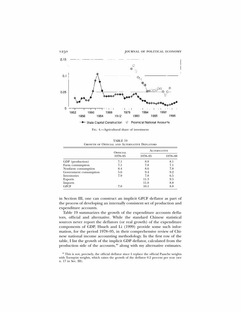
As emphasized in the Introduction, this paper focuses on the non-agricultural sector of the Chinese economy, using reproducible capitalalone as a measure of the capital stock. Although the published Chinesenational accounts do not provide information on the sectoral distri-bution of GFCF, the provincial accounts do. For the period 1978–95,Hsueh and Li (1999) report the sectoral distribution of gross fixedcapital formation in 26 provinces (all provinces other than Jiangxi,Guangdong, Hainan, and Tibet), accounting for an average of 78 per-cent of the annual value of national GFCF. I assume that aggregateGFCF during this time period has the same agricultural/nonagriculturaldistribution and extend the series forward by assuming that investmentshares in 1996 and 1997 were the same as in 1995. For the period1952–77, I draw on data in the CSY on the sectoral distribution of thegross fixed capital formation of state-owned units, which accounted foran average of 57 percent of the annual value of national GFCF duringthis period, to allocate the overall national fixed capital formation be-tween the agricultural and nonagricultural sectors of the economy. Asshown in figure 4, the proportion of state enterprise investment inagriculture is well below the provincial average (which includes theactivity of collective enterprises), so my use of state enterprise investmentto allocate investment during the period 1952–77 produces a discon-tinuity in 1978, when, as I switch to the provincial sample, the proportionof investment in agriculture jumps. This introduces a slight downwardbias into my estimate of capital growth in the nonagricultural sector.
With a measure of nonagricultural investment in hand, it is necessaryto derive an appropriate fixed capital formation deflator. The officialdeflator for GFCF is presumably an inappropriate choice since it relieson enterprise output deflators39 and is, consequently, likely to be char-acterized by the same understatement of inflation that plagues the Peo-ple’s Republic’s production estimates. An alternative independent priceindex is available in the form of the price index of investment, but thisindex has been available only since 1990, which does not provide asufficiently long time series. A third approach is possible: exploiting thenational income accounting identity equating the GDP deflator calcu-lated from the production accounts with the same deflator calculatedfrom the expenditure accounts. Alternative price indices for the non-capital components of final expenditure are available or are easily con-structed. Combining them with the revised production deflators used
39 Most of capital formation is construction (see below), which is deflated using theimplicit enterprise output deflator for the construction industry (Hsueh and Li 1999, p.148).
1250 journal of political economy
Fig. 4.—Agricultural share of investment
TABLE 19Growth of Official and Alternative Deflators
Official1978–95
Alternative
1978–95 1978–98
GDP (production) 7.1 8.9 8.1Farm consumption 7.1 7.8 7.1Nonfarm consumption 8.4 8.6 7.8Government consumption 5.6 9.4 9.2Inventories 7.9 7.8 6.5Exports 11.3 9.5Imports 11.0 8.8GFCF 7.0 10.1 8.8
in Section III, one can construct an implicit GFCF deflator as part ofthe process of developing an internally consistent set of production andexpenditure accounts.
Table 19 summarizes the growth of the expenditure accounts defla-tors, official and alternative. While the standard Chinese statisticalsources never report the deflators (or real growth) of the expenditurecomponents of GDP, Hsueh and Li (1999) provide some such infor-mation, for the period 1978–95, in their comprehensive review of Chi-nese national income accounting methodology. In the first row of thetable, I list the growth of the implicit GDP deflator, calculated from theproduction side of the accounts,40 along with my alternative estimates.
40 This is not, precisely, the official deflator since I replace the official Paasche weightswith Tornqvist weights, which raises the growth of the deflator 0.2 percent per year (seen. 17 in Sec. III).

productivity growth 1251
The expenditure share weighted average of the growth of the compo-nent deflators should equal this number. To begin with the simplestitem, private consumption expenditures, the Chinese national accountsdeflate them using various components of the CPI, plus the implicitenterprise deflator for construction.41 I replace the official deflators withthe rural and urban CPIs,42 which report very similar inflation rates.
I now turn to government consumption. The official (Hsueh and Li1999, p. 148) methodology is to deflate government employee salariesby the consumption basket of those workers (!) and the goods andservice components of government purchases using the retail and ser-vice price indices. Not only is this approach grossly incorrect, it is also,apparently, not implemented. At 5.6 percent per year, the growth of theofficial government expenditure deflator is well below the growth ofthe retail price index, the CPIs, or the (CPI) service price index. Theextremely slow growth of this deflator plays an important role in off-setting the high inflation recorded in other components of the expen-diture accounts, thereby bringing the official expenditure accounts inline with the production side. To replace the official deflator, I calculatethe share of employee salaries (taken as the value of government outputon the production side of the accounts) in government expendituresand arbitrarily divide the remainder, about 80 percent of the total,equally between purchases of goods and services. I then use theseweights to construct an expenditure deflator by combining the growthof the average wage of staff and workers in government and party agen-cies and social organizations43 with the growth of the retail and servicesprice indices.
With regard to inventories, the official deflator divides inventory ac-cumulation into agricultural, industrial, and commercial componentsand deflates them using price indices such as the farm and sidelineproducts procurement price index. I adopt a similar approach, usingthe detailed capital formation accounts of the 26-province sample notedearlier to separate inventory accumulation into primary, secondary, andtertiary sectors, which I then deflate using the farm and sideline prod-ucts, ex-factory, and retail price indices, respectively. It is reassuring thatmy measure of overall inventory inflation is close to the official estimate.Finally, for exports and imports, no official deflator that I know of hasbeen circulated. From earlier work (Young 1999), I have quantity andvalue data on Hong Kong’s trade with the Mainland during the period
41 Peculiarly, the consumption accounts include an adjustment for the depreciation ofprivate housing (Hsueh and Li 1999, p. 147).
42 The rural CPI is available only from 1984 on. I extend it back to 1978 using thegrowth of the urban CPI.
43 Less a 1.1 percent per year adjustment to reflect the changing characteristics ofworkers, as per my analysis in the preceding section.

1252 journal of political economy
1984–96 broken down into 823 consistent import and 899 consistentexport product categories. I use these data to construct a weighted unitvalue index for that period and extend the analysis to the years 1996–98and 1981–84 using data on the values and quantities of principal importand export products published in the CSY.44 For the period 1978–81, Iuse the retail price index to deflate both imports and exports. Theimport and export price indices show about 9 percent inflation per year,although the movement in dollar prices is considerably less, since theeffective yuan/dollar exchange rate (computed by dividing the value ofexports and imports in yuan by their value in dollars, as reported inthe CSY) depreciates 7.9 percent per year.
Finally, I turn to fixed capital formation. The official deflator increases7.0 percent per year between 1978 and 1995. Taking as given my esti-mates for the other elements of the expenditure and production ac-counts, I produce an alternative GFCF deflator, as a balancing residual,which grows 10.1 percent per year during the same period. It is inter-esting to note that the official deflator, which relies heavily on the en-terprise deflators in secondary industry, shows about 0.7 of the inflationrecorded in the alternative GFCF price index, which agrees with myestimates of the bias in the implicit production deflators of the nationalaccounts (see the discussion in Sec. III and the analysis in Young [2000]).As another consistency check, I note that between 1978 and 1998 themachine-building industry component of the ex-factory price index in-creases 4.3 percent per year, and the unit cost of construction activity,calculated from data on state and overall construction costs,45 grows 10.6percent per year. Weighting them by the annual investment shares ofmachinery and construction (with construction accounting for about0.7 on average),46 one arrives at an annual GFCF inflation rate of 8.9percent for the 1978–98 period. This compares, very favorably, with the8.8 percent GFCF inflation rate for 1978–98 calculated, as a residual,in table 19. In sum, three independent ways of calculating the averagegrowth of the GFCF deflator all yield highly similar estimates.
44 The Hong Kong data account for an average of 30 and 19 percent of the value ofChinese exports and imports, respectively; the CSY data cover about two-thirds of the totalvalue of exports and imports in 1981–84 and one-third of their value in 1996–98. TheCSY data contain only about 150 export and 70 import categories. Consequently, for theperiod 1984–96, I rely on the Hong Kong data, which, despite their smaller share of thevalue of trade, contain much finer product detail.
45 I combine the construction component of the price index of investment, availablefor 1990–98, with data on the unit cost per square meter of state capital construction for1978–90, both as reported in the CSY.
46 I use the CSY data on fixed asset investment by use of funds (e.g., 1999 CSY, table6-1). These data include a category “other,” which encompasses noncapital costs such astraining, product research, etc. I remove these items, focusing on equipment and con-struction alone. According to Hsueh and Li (1999), many, but not all (e.g., research), ofthese elements are removed in producing the national accounts estimates of GFCF.
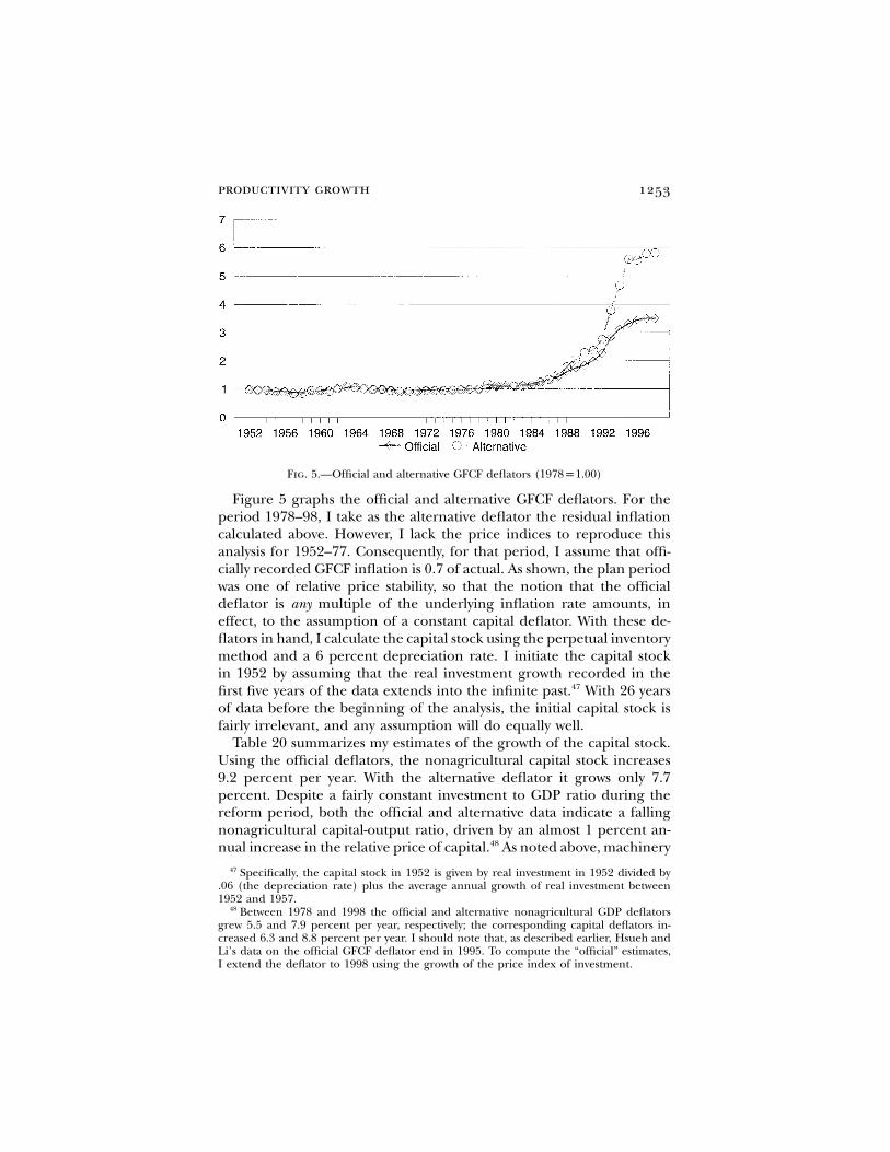
productivity growth 1253
Fig. 5.—Official and alternative GFCF deflators (1978p1.00)
Figure 5 graphs the official and alternative GFCF deflators. For theperiod 1978–98, I take as the alternative deflator the residual inflationcalculated above. However, I lack the price indices to reproduce thisanalysis for 1952–77. Consequently, for that period, I assume that offi-cially recorded GFCF inflation is 0.7 of actual. As shown, the plan periodwas one of relative price stability, so that the notion that the officialdeflator is any multiple of the underlying inflation rate amounts, ineffect, to the assumption of a constant capital deflator. With these de-flators in hand, I calculate the capital stock using the perpetual inventorymethod and a 6 percent depreciation rate. I initiate the capital stockin 1952 by assuming that the real investment growth recorded in thefirst five years of the data extends into the infinite past.47 With 26 yearsof data before the beginning of the analysis, the initial capital stock isfairly irrelevant, and any assumption will do equally well.
Table 20 summarizes my estimates of the growth of the capital stock.Using the official deflators, the nonagricultural capital stock increases9.2 percent per year. With the alternative deflator it grows only 7.7percent. Despite a fairly constant investment to GDP ratio during thereform period, both the official and alternative data indicate a fallingnonagricultural capital-output ratio, driven by an almost 1 percent an-nual increase in the relative price of capital.48 As noted above, machinery
47 Specifically, the capital stock in 1952 is given by real investment in 1952 divided by.06 (the depreciation rate) plus the average annual growth of real investment between1952 and 1957.
48 Between 1978 and 1998 the official and alternative nonagricultural GDP deflatorsgrew 5.5 and 7.9 percent per year, respectively; the corresponding capital deflators in-creased 6.3 and 8.8 percent per year. I should note that, as described earlier, Hsueh andLi’s data on the official GFCF deflator end in 1995. To compute the “official” estimates,I extend the deflator to 1998 using the growth of the price index of investment.

1254 journal of political economy
TABLE 20Nonagricultural Growth Rates (1978–98)
Capital Capital/Output
Official Data 9.2 �1.4Alternative 7.7 �.4
prices are rising relatively slowly, but the growth of the price of con-struction (whether measured officially or with alternative price indices)is very high, and construction dominates fixed capital formation.
VII. Factor Income Shares
Table 21 reports the ratio of compensation of employees to GDP atfactor cost in the People’s Republic, estimated using data from thenational accounts and input-output tables. As the reader can see, thefigures produced by the two sources are in broad agreement, althoughthe data in the input-output tables are quite volatile. The overall econ-omywide share of labor appears to be about 0.6, whereas in the non-agricultural sector it averages slightly below 0.5. At first glance, thesefigures appear to be somewhat low. As shown in table 22, in my 1995analysis of total factor productivity growth in the NICs, for example, Iused (adjusted) shares of labor in nonagricultural GDP on the orderof 0.6, 0.7, and even 0.75. Only in the case of Singapore did my estimateof the share of labor in nonagricultural activity fall as low as 0.5. Thesefigures, however, involve a modification of the underlying data. In table22, I also report the actual share of labor, that is, compensation ofemployees divided by GDP at factor cost, recorded by the national ac-counts and input-output tables of the NICs. At this level, the NICs arequite similar to the People’s Republic and to each other as well, withnonagricultural labor shares of 0.5 appearing to be the norm ratherthan the exception. To understand the adjustments I made, why theseadjustments were so minimal for Singapore and so substantial for theother economies and why no such adjustments are necessary for China,requires some explanation of the methods of the national accounts.
While the standard precepts of national income accounting requirethe imputation of some sources of income (e.g., the implicit rental onowner-occupied housing), they explicitly exclude such imputations inthe case of labor. “Compensation of employees,” as defined in the Systemof National Accounts, includes all wages, salaries, and supplementsearned by employees, the value of any income in-kind (lodging, etc.)they receive from their employers, and employer payments for theirsocial or private pensions. The implicit labor income of proprietors,unpaid family members, and the self-employed is supposed to be cap-

productivity growth 1255
TABLE 21Share of Labor in GDP at Factor Cost
National Accounts Input-Output Tables
GDP Nonagriculture GDP Nonagriculture
1978 .57 .421979 .59 .421980 .58 .431981 .60 .431982 .61 .441983 .61 .431984 .61 .441985 .60 .451986 .60 .461987 .59 .46 .60 .491988 .59 .471989 .59 .471990 .61 .49 .63 .521991 .60 .491992 .58 .48 .52 .401993 .59 .501994 .59 .511995 .61 .53 .54 .4419961997 .63 .56Average .60 .46 .58 .46
Note.—Input-output data for 1987 and 1990 are calculated from GDP at market prices and include under laborremuneration a residual category, “other,” consisting of some payments to labor and elements of enterprise materialconsumption.
TABLE 22Nonagricultural Labor Shares in the NICs (as Estimated in Young [1995])
Adjusted Unadjusted
HongKong Singapore
SouthKorea Taiwan
HongKong Singapore
SouthKorea Taiwan
1961 .62 .501966 .74 .551970 .66 .50 .69 .74 .56 .39 .47 .531975 .67 .63 .55 .451980 .57 .53 .76 .74 .49 .44 .50 .551985 .62 .70 .53 .491990 .60 .48 .78 .76 .52 .43 .56 .59Average .62 .50 .71 .75 .53 .42 .49 .56
Note.—Hong Kong data for 1970 on refer to the year plus one, e.g., 1971 instead of 1970. Hong Kong and Singaporedata refer to the entire economy, but the agricultural sectors are negligible.
tured, along with elements of the return to capital, under items suchas “income from unincorporated enterprises” (United Nations 1953).Since compensation of employees is restricted to employees, a naturaladjustment suggests itself: Impute to each nonemployee worker anhourly wage equal to the average hourly wage of employees with thesame age, sex, and educational characteristics. Aggregating across em-
1256 journal of political economy
ployee and nonemployee hours of work then provides an estimate oftotal explicit and implicit labor income. Multiplying the unadjustedshare of labor (compensation of employees over GDP at factor cost) inthe national accounts by one plus the ratio of implicit to explicit laborincome yields an estimate of the “true” share of labor.49 This is theprocedure I used in my 1995 analysis of the NICs. Unfortunately, itsystematically overstates the share of labor.
While national income accountants are not supposed to impute laborincome to nonemployees, in practice they do so, albeit unintentionally.To understand why, the reader might consider how he or she would goabout constructing an estimate of total compensation of employees ina data-poor developing country. The cost shares of large incorporatedenterprises are somewhat known, from sectoral surveys or tax records.In the case of small unincorporated enterprises, however, officials havelittle data, since the costs of data collection and monitoring limit theinformation, where it exists, to the most basic items, for example, de-clared output. Bereft of data, the national income accountant can as-sume either that (a) unincorporated enterprises pay no compensationto employees or that (b) the share of compensation of employees intheir total output is the same as that appearing in larger incorporatedenterprises. The latter assumption is more palatable and appears to beused in practice (see, e.g., Republic of China 1997, pp. 235–39). Sincethe share of unpaid workers in small firms is substantially higher thanin large firms, this procedure automatically imputes labor income tothe unpaid workers of small firms. In table 23, I list my 1995 estimatesof the adjusted share of labor in sectors such as wholesale and retailtrade and personal, social, and community services, which have largenumbers of nonemployee workers. Imputing an implicit income to un-paid workers frequently results in a labor share exceeding one as pay-ments to labor more than exhaust the total output of the sector.50 Thisis precisely what would arise if one double-counted the implicit incomeof unpaid workers.51
The data on compensation of employees reported by national income
49 One cannot use the estimates of implicit and explicit labor income drawn from laborforce survey and census data directly, since they typically do not include income in-kindor pensions. Multiplying by the national accounts estimate of compensation of employeesscales for these factors, as well as adjusts for any inconsistency between the overall levelof employee income reported by workers and firms.
50 The trends in the share of labor derive from the trends in the share of self-employedworkers (falling in wholesale and retail trade and rising in community, social, and personalservices) as the unadjusted national accounts estimates of compensation of employeesover GDP at factor cost are fairly constant.
51 In a similar vein, Denison (1979, app. G) found that business income (net of laborand material payments) in unincorporated enterprises in the United States was insufficientto cover an implicit labor and capital income equal to that of business sector employeesand incorporated enterprise capital.

productivity growth 1257
TABLE 23Nonagricultural Labor Shares by Sector in Korea and Taiwan
(Adjusted for Unpaid Workers, as Estimated by Young [1995])
Wholesale and Retail TradeCommunity, Social, and
Personal Services
A. South Korea
1970 1.20 .981975 1.01 .961980 .95 1.041985 .86 1.041990 .68 1.07
B. Taiwan
1966 1.50 .981970 1.92 1.061980 1.18 1.031990 1.09 1.02
accountants lie somewhere between the accounting precepts of the Sys-tem of National Accounts and a measure involving a full imputation ofthe implicit labor income of unpaid workers. As a lower labor share willtypically yield lower estimates of total factor productivity growth, to avoidcriticism on this dimension, in Young (1995), I assumed that the nationalaccounts followed, precisely, the conventions of the System of NationalAccounts and made a full adjustment for the implicit income of unpaidworkers. The difference between Singapore and the other economiesdoes not lie in the national income data, but rather in the fact thatSingapore has far fewer unpaid workers operating in small family-runenterprises. While my labor share estimates for Singapore are oftencriticized as being too low, it is more likely the case that, if anything,the estimates for the other economies are too high.
In the People’s Republic, self-employment is fairly rare.52 Moreover,the Chinese national accounts explicitly impute labor income to the self-employed, assuming that in industrial and construction enterprises inwhich self-employment is found, all income is labor income, and goingso far as to conclude that the entire output of some sectors (e.g., personaland social services) contains no net capital income component what-soever, allocating all of the output of the sector between compensationof employees and depreciation (see Hsueh and Li 1999, pp. 111, 114–15,123). Consequently, there is no reason to modify the reported Chineseestimates of the share of labor. The share of labor in the nonagriculturaleconomy in China is similar to that reported in other economies. Onceadjustment is made for unpaid workers, the ratios of other economies
52 According to the 1999 CSY (table 5-4), self-employed individuals accounted for only3 percent of the working population in 1990. This figure rises to 9 percent by 1998.
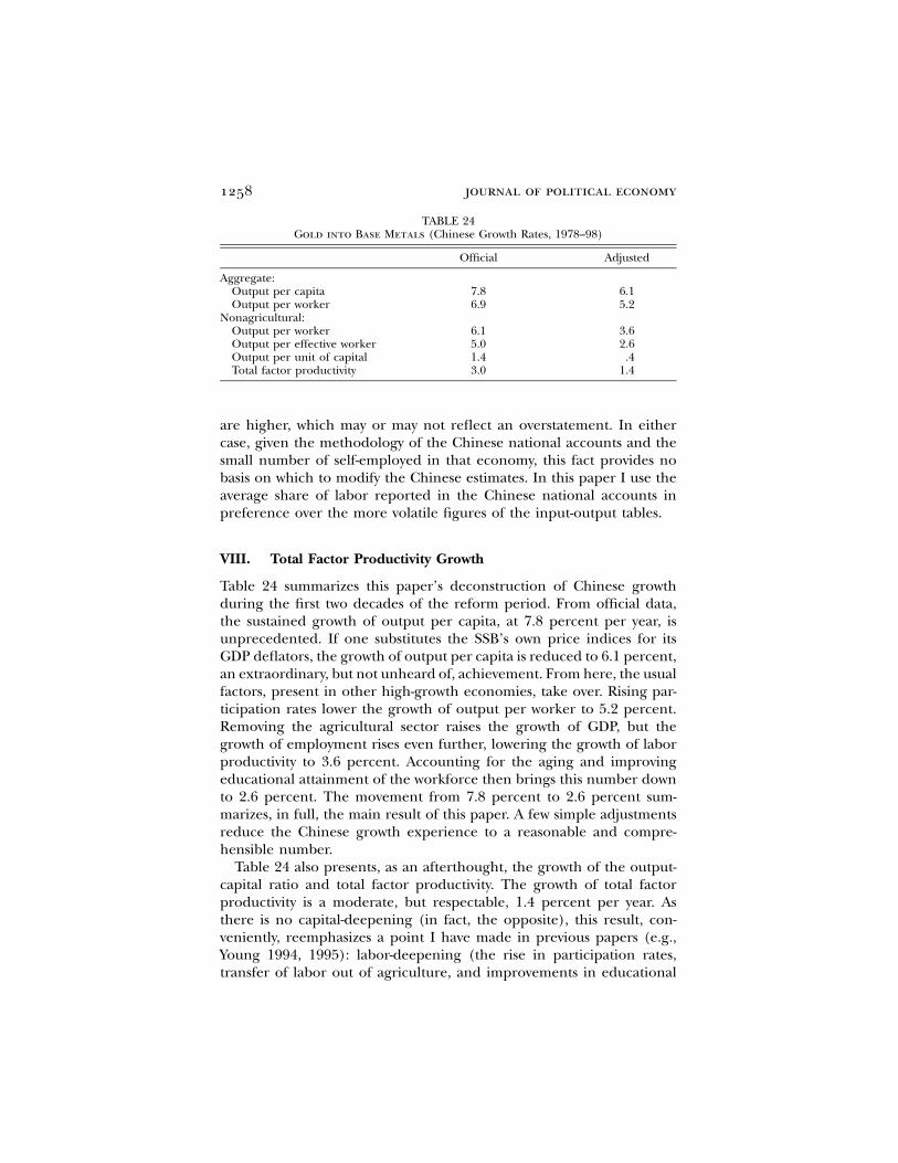
1258 journal of political economy
TABLE 24Gold into Base Metals (Chinese Growth Rates, 1978–98)
Official Adjusted
Aggregate:Output per capita 7.8 6.1Output per worker 6.9 5.2
Nonagricultural:Output per worker 6.1 3.6Output per effective worker 5.0 2.6Output per unit of capital 1.4 .4Total factor productivity 3.0 1.4
are higher, which may or may not reflect an overstatement. In eithercase, given the methodology of the Chinese national accounts and thesmall number of self-employed in that economy, this fact provides nobasis on which to modify the Chinese estimates. In this paper I use theaverage share of labor reported in the Chinese national accounts inpreference over the more volatile figures of the input-output tables.
VIII. Total Factor Productivity Growth
Table 24 summarizes this paper’s deconstruction of Chinese growthduring the first two decades of the reform period. From official data,the sustained growth of output per capita, at 7.8 percent per year, isunprecedented. If one substitutes the SSB’s own price indices for itsGDP deflators, the growth of output per capita is reduced to 6.1 percent,an extraordinary, but not unheard of, achievement. From here, the usualfactors, present in other high-growth economies, take over. Rising par-ticipation rates lower the growth of output per worker to 5.2 percent.Removing the agricultural sector raises the growth of GDP, but thegrowth of employment rises even further, lowering the growth of laborproductivity to 3.6 percent. Accounting for the aging and improvingeducational attainment of the workforce then brings this number downto 2.6 percent. The movement from 7.8 percent to 2.6 percent sum-marizes, in full, the main result of this paper. A few simple adjustmentsreduce the Chinese growth experience to a reasonable and compre-hensible number.
Table 24 also presents, as an afterthought, the growth of the output-capital ratio and total factor productivity. The growth of total factorproductivity is a moderate, but respectable, 1.4 percent per year. Asthere is no capital-deepening (in fact, the opposite), this result, con-veniently, reemphasizes a point I have made in previous papers (e.g.,Young 1994, 1995): labor-deepening (the rise in participation rates,transfer of labor out of agriculture, and improvements in educational

productivity growth 1259
attainment) and not capital-deepening is the key force explaining theextraordinary improvements in per capita living standards, in the pres-ence of moderate total factor productivity growth, achieved by the high-growth economies of East Asia.
The total factor productivity estimates of this paper should not, byany means, be taken as definitive. As table 24 shows, if one merely acceptsthe official GDP deflators but keeps all other elements of the analysisunchanged, the growth of total factor productivity jumps to 3.0 percent.Beyond this, an impressive range of estimates is possible. A quick anddirty optimist (Dr. Pangloss) might focus on the official (Laspeyres)growth of aggregate output per capita, denying the improvements inparticipation rates, ignoring changes in the composition of the work-force, and assuming a constant capital-output ratio and a 0.7 labor share(in line with the developed world), to produce a total factor productivitygrowth estimate of 5.6 percent per year. At the other extreme, the data-mining pessimist (Dr. Doom) might take my estimates as a baseline butlower the growth of nominal output by 1 percent (to correct for ex-aggeration), use the current official series on employment (with itsdiscontinuity in 1990), and weight the growth of human capital usingSingaporean relative wages in 1980, to produce a nonagricultural totalfactor productivity growth estimate of �0.4 percent per year. Theseparodies highlight the ease with which one can raise or lower estimatesof total factor productivity growth. It is hoped that the reader can makeuse of the lengthy discussion of data in this paper to adjust the estimatespresented in table 24 and attach to them the appropriate standard error.
IX. Conclusion
Having pressed through countless pages of dry data analysis, the readershould, arguably, be rewarded with some free-ranging interpretation andspeculation. The finding of moderate nonagricultural labor and totalfactor productivity growth can be viewed as either positive or negative.On the one hand, when contrasted with the experience of other re-forming economies, sustained 2.6 percent labor productivity growth canbe seen as nothing short of miraculous. On the other hand, given thatthe estimates presented in this paper are by no means the lowest possible(in particular, there is no adjustment for the exaggeration of nominalgrowth) and given the presumed inefficiency of central planning, onemight have expected greater gains in a “successfully” reforming econ-omy. In this regard, moderate productivity growth might be seen asreflecting enduring problems, such as the failure to reform state en-terprises and the inefficiencies introduced by local government inter-vention in industrial production and trade. Both interpretations arevalid since the Chinese glass is, clearly, both half full and half empty.

1260 journal of political economy
Like many magicians and alchemists, this paper buries its trickery inthe setting of the stage. Excluding agriculture, at the very beginning,from the analysis incorporates the transfer of labor out of that sectoras an input, while excluding agricultural total factor productivity growthand the efficiency gains brought about by movement of labor from themeasurement of output. The sustained growth of agricultural outputduring the reform period, in light of its rapidly declining share of thelabor force, is a testament to the misguided nature of plan policies thatkept the peasantry tied up in agriculture, by restricting rural-urban mi-gration and limiting the development of rural nonagricultural activity,while saddling it with inefficient and alien organizational structures.The reversal of these policies may be one of the greatest, and easiest,achievements of the reforms, although agriculture remains distorted inmany respects (e.g., with local procurement and price controls). Aproper analysis of the agricultural sector, lying well beyond the abilitiesof the techniques used in this paper, might find rapid productivitygrowth in that sector and large gains from the release of its pent-up“surplus” labor.
Along with rising participation rates, educational attainment, and cap-ital investment, the transfer of labor out of agriculture, whether drivenby productivity growth in that sector or the equalization of labor’s mar-ginal product with other sectors of the economy, has played an impor-tant role in the growth of economies such as Korea and Taiwan. It playsan equally significant role in fueling the growth of the People’s Republic.Despite the popular academic emphasis on industry and exports, adeeper understanding of the success of the world’s most rapidly growingeconomies may lie in that most fundamental of development topics:agriculture, land, and the peasant.
References
Chan, Kam Wing. “Urbanization and Rural-Urban Migration in China since1982.” Modern China 20 (July 1994): 243–81.
Chen, Dong, and Zhili Niu, eds. Practical Manual on Economic Statistics of China(Zhongguo tongji shiyong daquan). Beijing: China People’s Univ. Pubs., 1989.
Chen, Nai-ruenn. Chinese Economic Statistics: A Handbook for Mainland China. Chi-cago: Aldine, 1967.
Christensen, Laurits R.; Jorgensen, Dale W.; and Lau, Lawrence J. “Transcen-dental Logarithmic Production Frontiers.” Rev. Econ. and Statis. 55 (February1973): 28–45.
Denison, Edward F. Accounting for Slower Economic Growth: The United States in the1970’s. Washington: Brookings Inst., 1979.
Hsueh, Tien-tung, and Li, Qiang, eds. China’s National Income, 1952–1995. Boul-der, Colo.: Westview, 1999.
Hsueh, Tien-tung; Li, Qiang; and Liu, Shucheng, eds. China’s Provincial Statistics,1949–1989. Boulder, Colo.: Westview, 1993.
productivity growth 1261
Kim, Kwang-suk, and Park, Joon-kyung. Sources of Economic Growth in Korea,1963–1982. Seoul: Korea Development Inst., 1985.
People’s Republic of China. State Statistical Bureau. China Population StatisticsYearbook (Zhongguo renkou tongji nianjian). Beijing: China Statis. Pub. House,annual issues.
———. China Statistical Yearbook (Zhongguo tongji nianjian). Beijing: China Statis.Pub. House, annual issues.
———. 1982 Population Census of China (Zhongguo 1982 nian renkou pucha ziliao).Beijing: China Statis. Pub. House, 1982.
———. Tabulations of China 1% Population Sample Survey (Zhongguo 1987 nian1% renkou chouyang diaocha ziliao). Beijing: China Statis. Pub. House, 1988.
———. Tabulation on the 1990 Population Census of the People’s Republic of China(Zhongguo 1990 nian renkou tongji ziliao). Beijing: China Statis. Pub. House,1993.
———. 1995 nian quanguo 1% renkou chouyang diaocha ziliao. Beijing: China Statis.Pub. House, 1995.
Republic of China. National Income in Taiwan Area of the Republic of China, 1997.Taipei: Directorate-General Budget, Accounting and Statis., 1997.
Ruoen, Ren. “China’s Economic Performance in International Perspective.”Manuscript. Paris: OECD Development Centre, October 1995.
Summers, Robert, and Heston, Alan. “Append 5.6: Appendix Table of Contentsfor a Space-Time System of National Accounts aka Penn World Table 5.6.”Text file accompanying Penn World Tables version 5.6. December 1994. http://www.nber.org/pub/pwt56/ascii/append.56.
United Nations. Department of Economic Affairs. A System of National Accountsand Supporting Tables. New York: United Nations, 1953.
Woo, Wing Thye. “Chinese Economic Growth: Sources and Prospects.” Manu-script. Davis: Univ. California, October 1995.
Young, Alwyn. “Lessons from the East Asian NICS: A Contrarian View.” EuropeanEcon. Rev. 38 (April 1994): 964–73.
———. “The Tyranny of Numbers: Confronting the Statistical Realities of theEast Asian Growth Experience.” Q.J.E. 110 (August 1995): 641–80.
———. “Transport, Processing and Information: Value Added and the CircuitousMovement of Goods.” Manuscript. Chicago: Univ. Chicago, May 1999.
———. “Gold into Base Metals: Productivity Growth in the People’s Republicof China during the Reform Period.” Working Paper no. 7856. Cambridge,Mass.: NBER, August 2000.