Good practice guide for the calibration of EDMs on baselines · Good practice guide for the calibration of ... 3.5 Mounting of the EDM and the reflector ... A calibration measurement

SURVEYING Good practice guide EMRP JRP SIB60 Dissemination level: Public

Page 1 of 30 Version: V1.0 Status: Public © SURVEYING JRP-Consortium 2016

Good practice guide for the calibration of electro-optic distance meters on baselines


Page 2 of 30 Version: V1.0 Status: Public © SURVEYING JRP-Consortium 2016

Imprint

Authors: Milena Astrua1

Thomas Fordell2 Christa Homann3

Jorma Jokela4 Wolfgang Niemeier3 Florian Pollinger5

Dieter Tengen3

Jean-Pierre Wallerand6 Massimo Zucco1

1Instituto Nazionale di Ricercia Metrologica (INRIM), Strada delle Cacce 91, 10135 Torino, Italy 2VTT Technical Research Centre of Finland Ltd, Centre for Metrology MIKES, P.O. Box 1000, FI-02044 VTT, Finland 3Technische Universität Braunschweig, Institut für Geodäsie und Photogrammetrie, Pockelsstraße 3, 38106 Braunschweig, Germany 4Finnish Geospatial Research Institute (FGI), Geodeetinrinne 2, 02430 Masala, Finland 5Physikalisch-Technische Bundesanstalt (PTB), Bundesallee 100, 38116 Braunschweig, Germany 6Conservatoire National des Arts et Métiers (CNAM), 292 rue Saint-Martin, 75141 Paris Cédex 03, France

Contact email: [email protected]

These good practice guidelines were developed in 2016 by the JRP SIB60 “Metrology for Long Distance Surveying”

as part of the European Metrology Research Programme EMRP run by EURAMET e.V. All procedures were developed with best knowledge.

Neither the authors nor EURAMET e.V., however, can be held accountable for any damage caused by the application of these guidelines.

The good practice guide may not be altered or copied as excerpts without written consent of the

author team. The good practice guide as a whole can be freely distributed.

Braunschweig, September 16, 2016


Page 3 of 30 Version: V1.0 Status: Public © SURVEYING Consortium 2016

Contents

Objectives ........................................................................................................................................................ 4

1 SI traceability and concept of measurement uncertainty ......................................................................... 5

2 Requirements for reference baselines ..................................................................................................... 6

2.1 Location ................................................................................................................................................. 6 2.2 Construction of pillars ........................................................................................................................... 6 2.3 Meteorological sensor network ............................................................................................................ 7

3 Recommendations for Calibration Measurements ................................................................................... 8

3.1 Introduction ........................................................................................................................................... 8 3.2 Field book .............................................................................................................................................. 8 3.3 Synchronisation ..................................................................................................................................... 8 3.4 Meteorological compensation............................................................................................................... 8 3.5 Mounting of the EDM and the reflector ................................................................................................ 8 3.6 Distance observations ........................................................................................................................... 9

4 Data Processing ..................................................................................................................................... 10

4.1 General considerations on the processing strategy ............................................................................ 10 4.2 Components of a suitable 3D adjustment model ................................................................................ 11

5 Measurement uncertainty ..................................................................................................................... 14

5.1 Survey on contributions ...................................................................................................................... 14 5.2 Influence of the refractive index ......................................................................................................... 14 5.3 Influence of turbulence ....................................................................................................................... 16 5.4 Projection of the reference point ........................................................................................................ 17 5.5 Uncertainty estimate of the calibration parameters ........................................................................... 18

6 Presentation of results ........................................................................................................................... 21

7 Appendix ............................................................................................................................................... 23

7.1 Field book ............................................................................................................................................ 23 7.2 On traceability ..................................................................................................................................... 25

8 Literature ............................................................................................................................................... 28

Acknowledgements ........................................................................................................................................ 30



Objectives

The aim of this guideline is to provide a calibration strategy and a practical solution for surveyors and survey authorities who intend to or by law/regulations have to verify or calibrate their electro-optic distance meters (EDM) on a reference baseline. The content of this document is based on existing literature in the field, many years of practical experience of the authors in EDM calibration and on results of research performed by the joint research project (JRP) “SIB60 metrology for long distance surveying” as part of the European metrology research programme (EMRP) between July 2013 and June 2016

In this report the basic problem of traceability is discussed first to allow the surveyor to evaluate the standard of his calibration procedure with respect to the quality of the applied reference length information.

The specific objective of calibration measurements is typically to estimate the following calibration parameters: - Scale factor - Additional constant

For this task, a quality assessment of the used reference baseline is required and specific procedures for carrying out the observations, the data processing and their analysis are given here. As a result estimates for the calibration parameters “scale” and “additional constant” and the associated uncertainty are achieved.

The origin and magnitude of many uncertainty contributions are introduced, as well as a Monte Carlo based approach for the combination of adjustment-based coordinate analysis with uncertainty propagation.

Some information on alternative optical standards for realisation of SI units and the possibility of frequency calibration complete these guidelines.



1 SI traceability and concept of measurement uncertainty

Length measurements in surveying produce data that is stored and processed often for decades. They are the basis for cadastral archives or risk assessments. It is of utmost importance that the data taken by different instruments and observers is comparable, with a common scale and a common labelling of quality. According to the metre convention, all length measurements should be traceable to the SI definition of the metre:

“The metre is the length of the path travelled by light in vacuum during a time interval of 1/299 792 458 of a second.” (CGPM 1983, Resolution 1)

A calibration measurement must hence make sure that traceability to this definition is secured. The realisation of this definition and traceability of a particular device thereto can never be perfect. The standardized quantitative measure for the quality of a measurand with respect to its agreement with the SI definition is the measurement uncertainty according to the “Guide to the expression of uncertainty in measurement” (ISO/IEC Guide 98-3:2008).

“A measurement result is generally expressed as a single measured quantity value and a measurement uncertainty.” (ISO 17123-1:2010)

In case of EDM baseline calibrations, one important source of uncertainty is the fact that these measurements are not performed in vacuum but in air. The propagation speed of light depends on the medium. In case of air, models allow the derivation of the index of refraction from the measurement of thermodynamic properties like temperature, ambient pressure, humidity and carbon dioxide contents.

There are different approaches to establish SI traceability of geodetic baselines. One important perquisite for SI traceability is the correct estimate of the associated measurement uncertainty. In the appendix, two different examples for the realisation of traceability to the SI definition of the metre with low uncertainty are given.



2 Requirements for reference baselines

Following the discussion in section 1 on traceability, establishing a direct link to the SI definition with low measurement uncertainty is a laborious procedure and can only be made for selected so-called reference baselines. For setting up of a reference baseline that will serve calibration measurements for decades, some general requirements can be defined:

2.1 Location

For a reference baseline the location has to be selected carefully.

A stable geological area with homogeneous soil is required in order to guarantee long-term stability of pillars.

A shaded location with smooth winds results in low turbulence. If the reference baseline has to serve GNSS measurements as well, a free sky is required.

Effects due to human activity in the surrounding, e.g. machinery in buildings or traffic loads, have to be avoided.

To avoid reduction problems to common coordinate systems, the reference baseline should be almost horizontal. To guarantee a good intervisibility between pillars, a slight vertical gradient can help.

Regarding the length of the baseline, it should be related to the typical distances measured in practical surveying work. In general, the length of the reference baseline is in the range between 500 and 1000 m. A longer baseline is favourable for the determination of the scale factor with low uncertainty.

2.2 Construction of pillars

Regarding the purpose of the reference baselines, high effort is required for the set-up of all the pillars:

The centering system should guarantee an uncertainty of 0.1 mm and it has to serve for EDM equipment from different manufacturers.

Required is an identical instrument and target height or very precise information of tribrach zero points.

Typically six to eight pillars should be used and distributed so that all distances between a minimum and a maximum distance can be realised

For the construction of pillars, refer to DVW Merkblatt 8 (2014) where some specific requirements are given for the optimum construction principles and related problems.

A regular check of the stability of all pillars is mandatory, even if geological and soil conditions are good. This stability check has to be performed with an instrument whose measurement uncertainty should be considerably smaller than the suspected changes of pillar positions. The history of possible displacements of each pillar should be documented.



It should be mentioned that in principle, it is possible to design the baseline so that the measurement scale (“unit length”) of a specific device under test is sampled systematically (ISO17123-4:2012, Rüeger 1996). Thus the baseline verification is supposed to be sensitive to cyclic or short periodic errors as well. However, it is challenging to design baselines incorporating the various unit lengths of all devices on the market. More importantly, the typically small cyclic errors of modern instruments are much more reliably detectable by laboratory experiments. Therefore, it is advisable to use a reference system with considerably higher resolution e.g. an interference comparator, for this purpose. In case of a cyclic error, a typical sinusoidal deviation can be identified. This information can either be used to derive a correction formula. Alternatively the amplitude can also be used as an estimate of the magnitude of the uncertainty of this effect, assuming a rectangular probability distribution function.

2.3 Meteorological sensor network

To achieve a high accuracy for the estimation of the calibration parameters (scale factor and additional constant), the knowledge of the atmospheric conditions along the signal path is very important: an uncertainty of 1 °C on the average temperature along the optical path implies that a scale factor lower than 1 mm/km cannot be determined. For this reason a dense sensor field is desirable for a reference baseline, where air temperature, air pressure and relative humidity along the reference baseline are observed parallel to the calibration campaign. All sensors should be mounted so that they are not directly exposed to solar radiation, but with little thermal contact to their housing. In case of temperature, ventilation of the temperature mount is favourable (Eschelbach, 2009). A minimum requirement is the measurement of the temperature at two points, the device and target pillar.

The measurement of the environmental conditions should be frequently performed and recorded with a time stamp. Ideally, the data should be stored automatically. A reading at the beginning and at the end of a single pillar-pillar observation allows interpolation and the assignment of a temperature to one observation. For automatic reading, the thermal inertia of the sensors sets the sensible limit for temporal resolution. An interval of 30 s should provide sufficient resolution for typical scenarios.

It is furthermore advantageous to monitor irradiance in parallel. This quantity monitors the solar power transferred into the environment and is a suitable parameter to characterise homogeneity.



3 Recommendations for Calibration Measurements

3.1 Introduction

In regular intervals or due to legal prerequisites the responsible surveyor has to perform calibration or verification measurements, for example because he or she has to prove that the used equipment is in agreement with the specifications. It is recommended that these calibration measurements take place at least every year, since the validity of calibration parameters is restricted due to instrumental effects, like aging of electronic sensors, dynamic loads, and extreme weather conditions.. The history of calibration parameters for each instrument should be documented to monitor long-term aging effects and to identify sudden jumps as indicators for instrumental problems.

3.2 Field book

The field book to be used should contain all information on instruments used and their distribution as well as time stamps for every observation. An example for such a field book is given in the appendix.

3.3 Synchronisation

The operators must ensure that all clocks of the sensor network, of the operators and of the EDM under test are synchronized to enable secure assignment and post-processing of the various datasets. The accuracy of the synchronisation should be well below the refreshment interval of the environmental data.

3.4 Meteorological compensation

The correct application of velocity corrections, i.e. the compensation of the index of refraction is of high importance for a successful high accuracy calibration. The environmental sensor data can be entered into most contemporary EDMs and the internal velocity correction is immediately applied by software. In practice, however, this manual procedure is error-prone, provoking typos and extending the actual measurement significantly. Thus, it has turned out that it is more constructive to record the environmental data as described in section 2 and to apply the velocity correction only in the analysis of the whole dataset (in the office). To make this possible, it is important not to adopt any settings for temperature, air pressure and relative humidity within the instrument. It is recommended to use the settings for the standard atmosphere of each instrument instead. In this case, the scale for the internal meteorological correction should be “0 ppm”.

3.5 Mounting of the EDM and the reflector

For each instrument it is necessary to use the same prism that is used in daily operation. The prism constant given by the manufacturer of the prism has to be introduced into the instrument and recorded in the field book. It is expected that the prism constant is applied to the distances.



The forced centring of the instrument/prism is critical for high accuracy calibration measurements. Even in high quality grade tripods, eccentricities can amount up to several tenths of millimetres. If possible, the tribrachs should remain on the pillars during the whole calibration campaign. Thus, the position of the instrument/prism with respect to the reference point is always the same. If this is not possible, measures like the use of markers should be taken to ensure that the tribrachs have the same rotational position for each calibration.

All tribrachs should be carefully levelled. Suitable instruments are geodetic laser plummets with two perpendicular tubular levels and typical uncertainties in the order of 30 arcseconds.

Instrument and prism heights have to be measured and recorded. The difference should not exceed 15 mm, otherwise the prism carrier is unsuitable incapable for the calibration (see also the respective uncertainty estimate in section 0). To secure constant height offsets and to simplify the analysis, it is recommended to use identical tripods on all pillars.

The EDM and the target should be shadowed by an umbrella to avoid any effect due to direct sunshine and variable insulation effects. This also reduces bending effects due to temperature differences on each side of the instrument.

3.6 Distance observations

All distances have to be measured according to the specified order in the field book as defined by the intended analysis scheme (see section 4). Any automated target detection (ATR) should be turned off to avoid systematic artefacts. Instead, the centre of the reflector should be targeted manually by the observer. Each distance should be measured multiple times, typically 5 times independently. The instrument has to be newly adjusted to the prism each time.



4 Data Processing

4.1 General considerations on the processing strategy

The processing of the calibration measurements are based on two information sources:

Length information and height differences or 3D-coordinates of the pillars of the reference baseline as given in the calibration certificate of the baseline

set of actual observations during the calibration campaign as given in the field book

To determine the instrumental parameters (scale and additional constant) a least square adjustment is appropriate. At least two different approaches to determine these parameters are possible:

The parameters scale and the additional constant define a straight line, so the easiest way to determine the parameters is a linear regression: The EDM measurements are compared to constant distances calculated from the coordinates of the pillars and the differences are modelled as a straight line. The disadvantage of a linear regression model is that small centring errors will distort the results as the coordinates of the points are considered to be fixed.

If the pillar coordinates are included as parameters in the adjustment, it is possible that the coordinates of the pillars can be changed within the limits of the pillar uncertainties to fit the measurements. In such a 3D model, the slope distances are described as a function of the wanted instrumental parameters and the pillar coordinates. The 3D-adjustment should be carried out in a spherical coordinate system.

With almost horizontal distances in a straight line the coordinates of only one axis can be determined by distance observations. To work in 3D model additional information about the other axis has to be inserted into the adjustment model. An appropriate way is the introduction of additional observations: The coordinates of the pillars with variance information. A further advantage of this model is that the prior accuracy information on the pillar coordinates from the baseline determination can be taken into account.

Thus, the observations in latter model are:

Reduced slope distances between pillars.

Coordinates of pillars with covariance matrix to avoid rank deficiency. The covariance describes the accuracy of the pillar coordinate. Thus, it should be included in the modelling that the reference coordinates are imperfect as well. However, the uncertainty of the reference coordinates, determined by the reference measurement and the reproducibility of the centring should be low enough that the scale is not affected. A reasonable mathematical constraint for these experimental values are, e.g., standard deviations of σx = 0.1 mm, σy = 0.2 mm, σz = 0.1 mm, with y denoting the axis along the distance measurement.

The unknowns in this model are:

Y-component of point coordinates, determined by distances and prior coordinates

X- and Z- component of point coordinates, determined only by prior coordinates



instrumental parameters scale correction m and additive constant c

4.2 Components of a suitable 3D adjustment model

In the course of the JRP Surveying, a numerical analysis tool was developed based on the processing algorithms in this chapter. It has been implemented in the software tool “baseline” (Tengen and Niemeier, 2016). In the following major algorithmic steps will be discussed.

4.2.1 Functional model for the slope distances

A local spherical coordinate system with earth curvature is taken into consideration. It coincides with coordinate system of total stations and levelling. Projection corrections are not necessary. As side effect, however, the computation of slope distances sC from coordinates gets slightly more complicated

2 22

C 1 2 1 2

h

2 coss R h i R h t R h i R h t

s

R

with R representing the local earth radius, h1,2 the pillar heights, i and t respectively the instrument and target heights above the pillar reference points. The horizontal distances sh can be determined from the Cartesian pillar distances xi,j and yi,j by

2 1 2 1hcos cos *cosx x y y

R

s

RR

.

Since the angle is relatively small, it is numerically more stable to work with the first equation in the following numerically more stable approximation:

22

C 1 2 1 2

2 4 62 8

1 2 1 2

2 1 cos

22! 4! 6!

s h h i t R h i R h i

h h i t R h i R h i O

The observed distances s’ are corrected by a single common scale correction m and additive constant c for all observations

O 's m s c .

The basic functional model for the adjustment is hence finally the identity of computed slope distances sC with the corrected distances sO:

!

O Cs s .

Figure 1 Graphical representation of the instrument pararameters

c



4.2.2 Stochastic model for the observations

The 3D adjustment treats both the coordinate pillars and the observed distances as variables. The weighting between these observations must reflect the different uncertainties of this entrance data. The corrections deduced in the adjustment should be in the order of the assumed uncertainties. Larger deviations are an indication that the assumptions on the accuracy of the prior information should be reconsidered.

For the observed distances, prior accuracy information can be introduced either from previous calibrations or from specifications.

In case of the coordinates of the pillars, a covariance matrix Qxx,j for each pillar j should be introduced as derived from adjustment resp. determination of reference baseline coordinates /lengths.

𝑄𝑥𝑥,𝑗 = [

𝑞𝑥𝑥 𝑞𝑥𝑦 𝑞𝑥𝑧

𝑞𝑦𝑦 𝑞𝑦𝑧

𝑞𝑧𝑧

]

During the adjustment, the introduction of individual observation accuracies is a possible way to reweight blunders during the processing chain.

4.2.3 Correction of distances

It is mandatory to have corrections applied to the raw observations:

Atmospheric corrections:

First velocity correction: determine the refractive index from temperature, air pressure, and relative humidity and the approximation formula (Ciddor/Bönsch).

Beam curvature correction. Laser beam does not follow the chord between instrument and reflector, but follows a gentle arc with a radius 8 times larger than the earth radius (Rüeger, 1996)

Second speed correction. Local scale refractive index depends on altitude. Following the gentle arc, the laser beam passes closer to earth surface in its midpath.

Geometrical corrections:

If instrument and prism heights are different, parallax has to be considered (see also section 0).

4.2.4 Adjustment Model

A Gauss-Markov Model (Niemeier (2008)) can be used to determine the instrument parameter. The algorithms behind this analysis are sketched in the following:

Functional model:

�̂� = 𝑓(�̂�)



This equation is relating the adjusted observations �̂� explicitly to the estimated parameters �̂�. The measured observations 𝑠 have to be corrected by a residual 𝑣:

𝑠 + 𝑣 = 𝑓(�̂�)

The functional model is linearized explicitly by approximation to a first-order Taylor series expansion:

𝑠 + 𝑣 = 𝑓(�̂�) = 𝑓(𝑥0) + 𝐴𝑥

where 𝑥0 are a priori values of the parameters and 𝑥 are the estimated parameter corrections to the a

priori values: �̂� = 𝑥0 + 𝑥. The design matrix 𝐴 = [(𝜕𝑓

𝜕𝑥)

𝑥0

] contains the first derivative of function 𝑓()

with respect to parameters 𝑥.

𝑣 = 𝐴𝑥 − (𝑠 − 𝑓(𝑥0))

The linearized model with 𝑙 = (𝑠 − 𝑓(𝑥0)) then reads

𝑣 = 𝐴𝑥 − 𝑙

Stochastic model:

1

llP Q

The matrix 𝑄𝑠𝑠contains the covariance of the observations and the inverse matrix 𝑃 is called the weight matrix.

Least square minimization:

𝑣𝑇𝑃𝑣 = (𝐴𝑥 − 𝑙)𝑇𝑃(𝐴𝑥 − 𝑙) → min

Leading to

0Tv Pv

x

Solution:

1

ˆ T Tx A PA A Pl

𝑄𝑥�̂� = (𝐴𝑇𝑃𝐴)−1

The matrix 𝑄�̂��̂� contains the covariance of the adjusted parameters.



5 Measurement uncertainty

5.1 Survey on contributions

The calibration of offset and scale of an EDM is influenced by multiple uncertainty contributions. A survey is given in the Ishikawa diagram depicted in figure 2. According to GUM, all these contributions need to be quantified and their contribution to the calibration values determined by uncertainty propagation through the analysis. In this chapter, uncertainty magnitudes and a Monte Carlo based method for the determination of the expanded measurement uncertainty will be discussed.

Figure 2 Ishikawa diagram summarizing uncertainty contributions to the calibration process.

5.2 Influence of the refractive index

The uncertainty of the expressions by Ciddor or Bönsch and Potulski for the refractive index of air is at the level of a few parts in 10-8, but this requires temperature to be known within 10 mK, pressure within 4 Pa, relative humidity within 1 % and CO2 contents within 70 ppm. The uncertainty of the calibration of respective sensors is typically well below these. However, the uncertainty of the effective refractive index along the whole beam path is dominated by the challenge to sample the spatial and temporal gradients of these quantities directly.



For long distance surveying under rapidly changing conditions, a near continuous array of accurate and fast sensors would be needed exactly along the path of the EDM beam. The requirements for temperature and humidity are especially demanding. While substantial progress has been made in lessening the demands on temperature data by measuring at multiple wavelengths (Meiners-Hagen et al., 2016) and in realizing a spatially continuous measurement of temperature (Hieta et al., 2011) and humidity (Pollinger et al., 2012b) along the EDM path spectroscopically, these methods are not widely available yet. When the air parameters can only be measured at one or a few points around the EDM beam, knowledge of the size of gradients, especially for temperature, becomes very important for determining the measurement uncertainty.

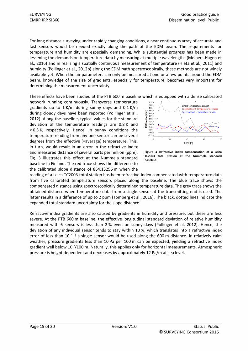
These effects have been studied at the PTB 600 m baseline which is equipped with a dense calibrated network running continuously. Transverse temperature gradients up to 1 K/m during sunny days and 0.1 K/m during cloudy days have been reported (Pollinger et al., 2012). Along the baseline, typical values for the standard deviation of the temperature readings are 0.8 K and < 0.3 K, respectively. Hence, in sunny conditions the temperature reading from any one sensor can be several degrees from the effective (=average) temperature. This, in turn, would result in an error in the refractive index and measured distance of several parts per million (ppm). Fig. 3 illustrates this effect at the Nummela standard baseline in Finland. The red trace shows the difference to the calibrated slope distance of 864.13256 m when the reading of a Leica TC2003 total station has been refractive-index-compensated with temperature data from five calibrated temperature sensors placed along the baseline. The blue trace shows the compensated distance using spectroscopically determined temperature data. The grey trace shows the obtained distance when temperature data from a single sensor at the transmitting end is used. The latter results in a difference of up to 2 ppm (Tomberg et al., 2016). The black, dotted lines indicate the expanded total standard uncertainty for the slope distance.

Refractive index gradients are also caused by gradients in humidity and pressure, but these are less severe. At the PTB 600 m baseline, the effective longitudinal standard deviation of relative humidity measured with 6 sensors is less than 2 % even on sunny days (Pollinger et al, 2012). Hence, the deviation of any individual sensor tends to stay within 10 %, which translates into a refractive index error of less than 10-7 if a single sensor would be used along the 600 m distance. In relatively calm weather, pressure gradients less than 10 Pa per 100 m can be expected, yielding a refractive index gradient well below 10-7/100 m. Naturally, this applies only for horizontal measurements. Atmospheric pressure is height dependent and decreases by approximately 12 Pa/m at sea level.

Figure 3 Refractive index compensation of a Leica TC2003 total station at the Nummela standard baseline.

Single temperature sensor Ensemble of 5 temperature sensors Spectrocopic temperature sensor



Regarding temporal gradients, pressure changes over the course of a normal day tend to be small, well below 100 Pa/d, yielding an estimate for the refractive index change due to pressure variations of <10-8/h. In the evening hours, humidity can change by several tens of percent in one hour, which gives a refractive index change of a few times 10-7/h. Finally, for temperature, a typical temporal gradient during the day is 1 K/h, which turns into 1∙10-6/h for the refractive index. In the morning and evening hours, the gradient can be several times higher; however, the passing of local rain shower can reduce the temperature by several degrees in, say, 15 minutes, giving a refractive index gradient up to 1∙10-5/h. This is illustrated in Fig. 4, which shows the average and standard deviation of five Pt-100 temperature sensors placed along the 864-m Nummela standard baseline. At about 15 o’clock, a rain shower lasting for about one hour dropped the temperature by 3 degrees in 20 minutes, the maximum gradient being around 15 K/h, which corresponds to 1∙10-5/h for the refractive index.

5.3 Influence of turbulence

The propagation of the laser beam in the atmosphere to measure optically distance is affected by turbulence caused by movement of the mass of air either caused by wind or by thermal exchanges between the ground and the air.

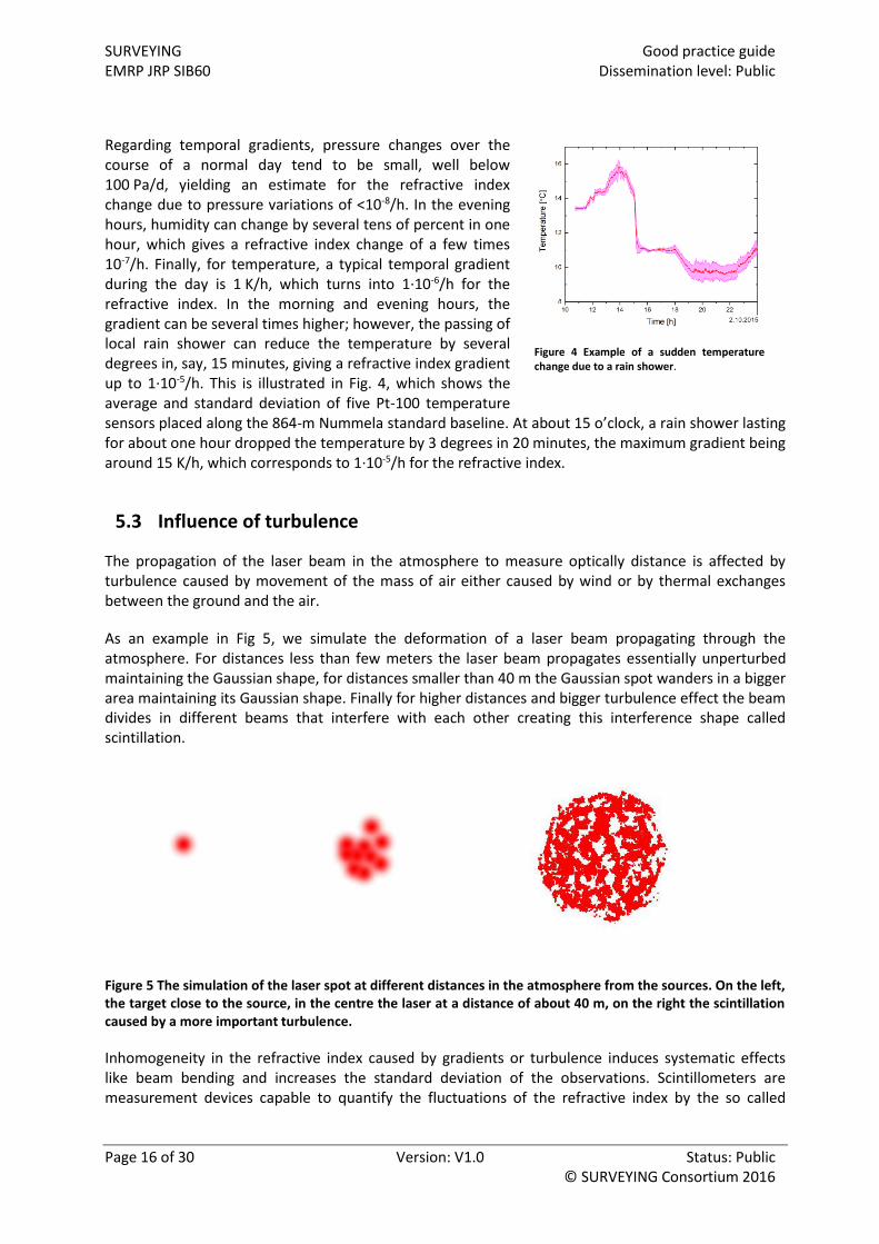
As an example in Fig 5, we simulate the deformation of a laser beam propagating through the atmosphere. For distances less than few meters the laser beam propagates essentially unperturbed maintaining the Gaussian shape, for distances smaller than 40 m the Gaussian spot wanders in a bigger area maintaining its Gaussian shape. Finally for higher distances and bigger turbulence effect the beam divides in different beams that interfere with each other creating this interference shape called scintillation.

Figure 5 The simulation of the laser spot at different distances in the atmosphere from the sources. On the left, the target close to the source, in the centre the laser at a distance of about 40 m, on the right the scintillation caused by a more important turbulence.

Inhomogeneity in the refractive index caused by gradients or turbulence induces systematic effects like beam bending and increases the standard deviation of the observations. Scintillometers are measurement devices capable to quantify the fluctuations of the refractive index by the so called

Figure 4 Example of a sudden temperature change due to a rain shower.



“structure constant of refractive index” Cn2. Quite Intense turbulence conditions (Cn

2 ≈ 5 10-13 m-2/3) correspond to typical standard deviations in the order of 10 µm for a distance of 80 m. This is effect is hence often negligible compared to other effects. For more turbulent conditions, however, the standard deviation can increase significantly.

A measurement of the wind speed can also used to deduce conclusions on the magnitude of these effects. For a length of approx. 80 m, a wind speed up to 3 m/s leads to a standard deviation of the order of 10 µm.

As a general recommendation, calibration measurements should only be performed if the weather conditions are stable. Generally speaking, direct sun exposure should be avoided if possible. A few hours after sunset more homogeneous conditions can be expected. Wind speed should be below 3 m/s. If measurable, the structure constant Cn

2 should be well below 10-13 m-2/3.

For a deepened treatment of the influence of turbulence one can refer, for example, to the work of Brunner, 1979, Böckem et al., 2000, Grabner and Kvicera, 2012, Konyaev et al., 2015, Yano et al., 2014, and Zucco et al., 2015.

5.4 Projection of the reference point

Levelling (requirement on accuracy)

The levelling accuracy depends on the minimum distance between the pillars. It is assumed that the pillars are in a horizontal straight line (see also figure 1).

∆𝑠 = √𝑠2 + ∆ℎ2 − 𝑠 ⇒ ∆ℎ = √∆𝑠 ∗ (2𝑠 − ∆𝑠)

Examples:

s = 18.78 m (the shortest distance baseline at the reference baseline of Neubiberg, Germany)

∆𝑠 = 0.1 𝑚𝑚 → ∆ℎ = 61𝑚𝑚

∆𝑠 = 0.01𝑚𝑚 → ∆ℎ = 17 𝑚𝑚

The requirements for the height determination are therefore moderate and can be met with reasonable effort. This refers to the instrument and prism heights, too.

Tribrach orientation

The uncertainty of geodetic-grade centrings are typically in the order of 20 µm or below. More critical are eccentricities of the tribrach reference point which can amount up to several tenths of a millimetre. It is important to mount tribrachs reproducibly on a baseline during a calibration and with respect to the reference value determination. Markers for the orientation can help to reduce this source of uncertainty.

Levelling the individual tribrachs should be performed with high quality geodetic laser plummets with two perpendicular tubular levels. For typical uncertainties in the order of 30 arcseconds, length deviations due to tilted EDMs and reflectors can be reduced to the order of 40 µm.



5.5 Uncertainty estimate of the calibration parameters

Uncertainty propagation for a 3D adjustment as discussed in chapter 4.2 is not straightforward. Monte Carlo methods which numerically repeat the analysis with randomly varying starting conditions are a suitable and well-established tool to propagate the contributing uncertainties.

Nowadays with efficient computers and good random number generators large samples are possible. Input variability is computed by deterministic, pseudorandom sequences, making it easy to test and re-run simulations.

One algorithm for the implementation of such an uncertainty propagation could be:

Define the functional relation between input data and quantity of interest (see chapter 4.2).

Use the uncertainty assessment of the various contributing quantities to define a domain of

possible input data.

Generate input data randomly from a probability distribution over the domain.

Perform a deterministic computation on the inputs and get the quantities of interest.

Aggregate and analyze the computed quantities of interest.

To demonstrate achievable measurement uncertainties for a calibration measurement, this procedure was performed for measurements at the baseline of PTB Braunschweig in the following discussion.

Each simulation consists of 1000 runs of the adjustment. Each time a new set of points and observations is generated. A forced centring is assumed so the coordinates may differ in each simulation according to the pillar centring variations. As a result the scale and the additional constant are determined in each run.

Steps per run:

Adopt centring variations to pillar coordinates

Consider instrument and target height

Calculate observations from coordinates

o Uncertainties of calibration data for EDM

o Uncertainties of atmospheric data for EDM

o Instrument accuracy

Adjust the observations

Store the results of the adjustment

The data of each run are collected. The results are stored in a vector, sorted by value and the following values are determined:

2,5 % lower limit 95 % significance level

16 % lower limit 68 % significance level, one standard deviation

50 % Median

84 % upper limit 68 % significance level, one standard deviation

97,5 % upper limit 95 % significance level



It should be noted that the quantiles can be interpreted independent from the distribution.

Based on the considerations before, the following entrance parameters were chosen for the uncertainty propagation:

Type A: based on statistical analysis of real observations during the measurement

In a real calibration measurement, the following quantities are acquired by multiple measurements. The derived mean value and standard deviation enter into the adjustment. For the simulations, also these “observations” were simulated based on the following assumptions for the uncertainties:

Observed distances: Every EDM under test is imperfect, e.g. due to electronic noise or mechanical design stability. The quality of the observation data limits of course also the uncertainty of the achievable correction parameters. To account for this effect, a selection of devices of typical different accuracy grades has been used for the simulations (c is the additional constant and m the scale factor):

Instrument Standard deviation of c [mm]

Standard deviation of m [ppm]

Ideal 0.0 0.0

ME 5000 0.2 0.2

EDM A 0.6 1.0

EDM B 1.0 2.0

EDM C 2.0 2.0

Atmospheric Parameters: The atmospheric parameters are observed by a temperature network. For the simulations, the following uncertainties and distributions are assumed reflecting the difficulty in sampling them with sufficient accuracy: Temperature: uniform distribution, σ = 0.8 K; 1 K ≈ 1 ppm

Pressure: uniform distribution, σ = 0.5 mbar; 1 mbar ≈ 0.3 ppm

Humidity: uniform distribution, σ = 5 %

Type B: based on prior knowledge

These uncertainty contributions are estimated based on other prior information like

1. Pillar and centring variations Uniform distribution, 0.1 mm

2. Instrument and target height Uniform distribution, 0.2 mm



The PTB baseline consists of 8 pillars with distances between 50 m and 600 m. All 28 different distances are measured 5 times, total 140 measurements. For each instrument 1000 adjustments were carried out.

The results for the additional constant and the scale are stored and sorted. To determine the quantile the 25th, 160th, 500th, 850th and 975th value was selected and is shown in the following tables.

Results: additional constant c in mm:

Instrument 2.5% 16% Median 84% 97.5%

ideal -0.05 -0.03 0.00 0.024 0.044

ME5000 -0.08 -0.04 0.00 0.04 0.08

EDM A -0.21 -0.10 0.00 0.11 0.21

EDM B -0.32 -0.16 0.00 0.18 0.33

EDM C -0.36 -0.17 0.00 0.19 0.35

Results: scale factor in ppm:

Instrument 2.5% 16% Median 84% 97.5%

ideal -0.32 -0.16 0.00 0.17 0.31

ME5000 -0.41 -0.20 -0.01 0.20 0.35

EDM A -0.82 -0.44 0.00 0.40 0.75

EDM B -1.02 -0.64 -0.01 0.56 1.12

EDM C -1.39 -0.74 -0.02 0.68 1.29



6 Presentation of results

The calibration result should be given as correction value with the expanded measurement uncertainty corresponding to a coverage interval of 95%, e.g.:

Scale factor = (0.10 ± 0.30) ppm

Additional constant c = (-4.800 ± 0.071) mm

The calibration certificate should also provide more detailed information, like a graphical representation of the adjustment result (figure 6), or a tabular compilation of the individual measurements (table 1).

Figure 6 Graphical representation of the adjustment result for the instrumental parameters

Reference distance [mm]



Table 1 List of measured distances, extract



7 Appendix

7.1 Field book

The following field book realized in a spreadsheet program collects all information required for the analysis of the calibration measurement.

Figure 7 General data

observers:

home institutes:

all clocks synchronised: yes

EDM:

automated data aquisition: no

reflector:

targeting method: manual

calibrated device: yes

calibration date:

calibration factors: offset / m: scale factor: further:

standard pressure / hPa:

standard temperature / °C:

standard humidity / %rf:

baseline:

baseline orientation with

respect to the starting point:

nominal pillar positions / m 0 50 100 150 250 350 500 600

centring method:

centring uncertainty (k=1):

level for alignment: type:

device height over reference

point / m

reflector height over reference

point / m

measurement date

Dates and operators

operators

uncertainty / m (k=1):

uncertainty / m (k=1):

uncertainty / deg (k=1):

Baseline data

Mounting and Alignment

Measurement method

Measurement method

Environmental correction - please use standard atmosphere!

calibration laboratory:



Figure 8 Sensor configuration

Figure 9 Environmental parameter observations

Figure 10 Distance observation sheet

Location type short identifier position / m device name/

specification

serial number date of

last calibration

starting point - measurement simultaneously with every data point

barometer p_start n.a. mbar

thermometer T_start n.a. K

humidity sensor RH_start n.a. %RH

barometer p_end n.a. mbar

thermometer T_end n.a. K

humidity sensor RH_end n.a. %RH

thermometer 1 T_long1 K



thermometer 1 T_lat1 K



thermometer 1 T_vert1 K



wind speed sensor v_wind

wind direction sensor v_direct

CO2 contents CO2 ppm

luxmeter Lux

measurement uncertainty of

last calibration (k=1)

end point - measurement simultaneously for every data point

longitudinal temperature gradient - measurement at least every 15 minutes

lateral gradient - measurement at least every 15 minutes

ancillary sensors - measurement at least every 15 minutes

to be shaded

by umbrella

to be shaded

by umbrella

vertical gradient - measurement at least every 15 minutes

Date Time overall p_start T_start RH_start p_end T_end RH_end T_long1 T_long2 T_long3 T_lat1 T_lat2 T_lat3 T_vert1 T_vert2 T_vert3 v_wind v_direct CO2 Lux

00.01.1900 00:00:00

00.01.1900 00:15:00

00.01.1900 00:30:00

00.01.1900 00:45:00

00.01.1900 01:00:00

00.01.1900 01:15:00

00.01.1900 01:30:00

00.01.1900 01:45:00

Final slope distances - all distances given shall be given in raw slope data, neither refractivity-compensated, nor reduced

Date time EDM position Reflector position p_start T_start RH_start p_end T_end RH_end Reading 1 Reading 2 Reading 3 Reading 4 Reading 5

00.01.1900 00:00:00

00.01.1900 00:00:00

00.01.1900 00:00:00

00.01.1900 00:00:00

00.01.1900 00:00:00

00.01.1900 00:00:00

00.01.1900 00:00:00

distance IDenvironmental conditions

(EDM position)

Dateenvironmental conditions

(reflector position)

distance for five manual readings



7.2 On traceability

7.2.1 Traceability chain: the example of the Nummela scale transfer

The establishment of traceability to the SI definition of the metre for reference lengths of baselines with low uncertainty is non-trivial. In this section, the approach of the Finnish Geospatial Research Institute (FGI) is introduced. The so-called Nummela scale transfer is an internationally acknowledged calibration service for geodetic baselines. It also demonstrates the increase of uncertainties in the different steps of the traceability chain.

The national metrology institute of Finland, VTT MIKES Metrology, performs the high-level realization of the definition of the metre using internationally recommended methods. VTT also calibrates FGI’s 1-metre-long quartz gauges, which transfer the traceable scale to FGI’s Väisälä interference comparator. A measurement setup and procedure combining white light and laser light in an interferometer for long gauge blocks is used (Lassila et al. 2003).

The length of a quartz gauge, known with 35 nm standard uncertainty, is multiplied in the (white-light) Väisälä interference comparator to realise longer distances. The design of FGI’s Nummela Standard Baseline allows a multiplication of 2 x 2 x 3 x 3 x 4 x 6 x 1 m = 864 m. Typical standard uncertainties are from 0.03 mm to 0.08 mm for the baseline lengths from 24 m to 864 m (Jokela 2014).

Projection measurements transfer the lengths between underground baseline benchmarks to lengths between centring equipment on above ground observation pillars, which are used in EDM calibrations. Owing to the optimal measurement geometry and best available measurement instruments the standard uncertainties after the projections remain smaller than 0.2 mm.

The FGI mostly uses a Kern ME5000 high-precision EDM equipment as a transfer standard for traceable scale transfer from Nummela to other geodetic baselines. The transfer standard is calibrated a few times at Nummela before and after the measurement at the scale transfer site, accompanied by before and after projections at Nummela. Figure 11 shows the procedure in more detail.

In processing meteorological data for EDM the FGI uses a computation method first proposed by Ciddor (1996), as recommended by the International Association of Geodesy (IAG, 2000). If using some of the formulas presented in the Kern ME5000 manual (Owens, Edlen, Barrel & Sears) instead, differences of up to 0.1 mm may occur in corrections.



Figure 11 Overview of calibration of transfer standard for scale transfer (Jokela 2014)

7.2.2 Alternative optical standards for the primary realisation of the SI unit metre in surveying

As mentioned in 1.1, even if an optical instrument is capable of measuring somehow the time of flight of a light beam between two points with an accuracy as high as possible, the estimation of the distance between these points will be degraded by the way of estimating the speed of light between these points. The classical way is based on local sensors that are expected to give estimation as close as possible of the effective atmospheric parameters all along the light beam. But even with a large effort in the sensor network, the uncertainty of such a sensor-based approximation of the effective environmental parameters remains limited (see chapter 5.1). Spectroscopic sampling of the effective environmental parameters can reduce the uncertainty significantly (Hieta, 2011).

Another alternative is to use the dispersion of air index (known thanks to air index formulas) between two separate wavelengths. By measuring the same distance simultaneously at two different wavelengths, the true distance can be deduced without measuring neither the air temperature nor the

air pressure. If L1 is the distance measured at wavelength 1 (taking the air index equal to unity), L2 the

distance measured at wavelength 2 (taking the air index equal to unity), the true distance L can be written as follow (with minor simplification):

L=L1+A(1 ,2 )x(L2-L1)

The A factor is a quantity deduced from air index formulas and that depends only on the value of the

two wavelengths chosen for the measurement (for 1=1064 nm and 2=532 nm A is equal to 21). This A factor acts also as an amplification factor of the dispersion of the distance measurement: the dispersion on (L2-L1) measurement is amplified by this factor A. This is the price to pay for air index compensation: the uncertainty on L2-L1 should be A times better than the global uncertainty reached

Weather variations along the path of measurement ?

Stability of the baseline ?

National standard baselinesection lengths (between

underground markers)

Projection measurements for calibrations

National standard baseline section lengths (aboveground, between

observation pillars)

EDM instrument observations for calibration (including

centring, levelling, targetting etc.)

Weather observations (t, p, rh%, CO2)

Instrument corrections for weather observations

Height differences for geometrical corrections

Observed and corrected baseline section lengths

Comparison, weighted

least-squares adjustment

EDMinstrument corrections

for the transfer standard• scale correction,• additive constant,• possible other;

• stability of results (calibrations before/after)?

Computation formulas for corrections for distances

Similar measurements and computations using the calibrated transfer standard

at the transfer site

Calibration programme

Calibration history (time series)



for the true distance. In the past, several units of such a device, known as Terrameter (Hugget, 1981) were realized and used for some critical applications. The principle of operation with millimetre level accuracy was demonstrated but no such instrument is in operation today.

Within the frame of the JRP Surveying this approach was revived using modern optical and recent advances in laser technology. The “TeleYAG” system (Meiners-Hagen et al., 2015) is a primary standard for baseline calibrations with measurement uncertainties on sub-millimetre level. It is now used in the German national metrology institute for the calibration of their baseline. A stronger focus on transportability and user-friendliness was put on the parallel not yet completed development of the TeleDiode system based on optoelectronic fibre technology (Guillory et al., 2016). The developers see the potential of the design to make an operational transportable instrument available to a broader application group in a near future.



8 Literature

Bönsch, G.; Potulski, E (1998). Measurement of the refractive index of air and comparison with modified Edlén's formulae. Metrologia 35, 133-139

Böckem, B.; Flach, P.; Weiss, A.; Hennes, M. (2000). Refraction influence analysis and investigations on automated elimination of refraction effects on geodetic measurements. Proc. of XVI IMEKO World Congress 2000

Brunner F.K. (1979). Vertical refraction angle derived from the variance of the angle-of-arrival fluctuations. Refractional Influences in Astrometry and Geodesy, pp. 227-238

Ciddor, P. E.; Hill, R. J. (1999): Refractive index of air: 2. Group index. Applied Optics, 38(1999)9, 1663-1667.

Ciddor, P. E. (2002): Refractive index of air: 3. The roles of CO2, H2O, and refractivity virials. Applied Optics, Vol. 41, No. 12, 2292-2298, 2002

Ciddor, P. E. (1996). Refractive index of air: New equations for the visible and near infrared, Appl. Opt. 35:9, 1566–1573.

DVW-Merkblatt 8 (2014). Vermessungspfeiler. Available online under http://www.dvw.de/dvw-iso/17515/vermessungspfeiler

Eschelbach, C. (2009). Refraktionskorrekturbestimmung durch Modellierung des Impuls und Wärmeflusses in der Rauhigkeitsschicht, Dissertation, Schriftenreihe des Studiengangs Geodäsie und Geoinformatik, Universität Karlsruhe (TH), Heft-Nr. 2009/1. 2009.

Grabner, M.; Kvicera V. (2012). Measurement of the Structure Constant of Refractivity at Optical Wavelengths Using a Scintillometer. Radioengineering 21, pp. 455-458

Guillory, J.; Šmid, R.; Garcia-Marquez, J.; Truong, D.; Alexandre, C.; Wallerand, J.-P. (2016). High resolution kilometric range optical telemetry in air by radio frequency phase measurement Review of Scientific Instruments 87, 075105

Heister, H. (2012): Die neuen Kalibrierbasis der UniBW München. AVN, 10/2012, p 336-343

Heunecke,O. (2015). Die neue Neubiberger Pfeilerstrecke, In: Zeitschrift für Geodäsie, Geoinformation und Landmanagement, ZFV, 2015, pp. 357-364.

Hieta, T.; Merimaa, M.; Vainio, M.; Seppä, J.; Lassila, A. (2011). High-precision diode-laser-based temperature measurement for air refractive index compensation Appl. Opt., , 50, pp. 5990-5998

Huggett, G (1981), Two-color terrameter, Tectonophysics 71, pp. 29 - 39

IAG (2000). IAG Resolution 3 adopted at the XXIIth General Assembly in Birmingham. J. Geodesy 74:1, 66–67.

ISO 17123-1:2010, Optics and optical instruments – Field procedures for testing geodetic and surveying instruments – Part 1: Theory (2010)

ISO 17123-4:2012, , Optics and optical instruments – Field procedures for testing geodetic and surveying instruments – Part 4: Electro-optical distance meters (EDM measurement to reflectors)

ISO/IEC Guide 98-3:2008, Uncertainty of measurement – Part 3: Guide to the expression of uncertainty in measurement (GUM:1995)

http://www.dvw.de/dvw-iso/17515/vermessungspfeiler

http://www.dvw.de/dvw-iso/17515/vermessungspfeiler



Jokela, J. (2014). Length in Geodesy – On Metrological Traceability of a Geospatial Measurand. Publ. Finn. Geod. Inst. 154. 240 p.

Konyaev, P. A.; Botygina N. N.; Antoshkin, L.V.; Emaleev, O.N.; Lukin, V. P. (2015). On Atmospheric Turbulence Structure Constant Measurements by a Passive Optical Method. Proc. SPIE Vol 9680, 968024

Lassila, A., Jokela, J., Poutanen, M., Xu, J. (2003). Absolute calibration of quartz bars of Väisälä interferometer by white light gauge block interferometer. Proc. XVII IMEKO World Congress, June 22–27, 2003, Dubrovnik, Croatia, p. 1886–1890.

Meiners-Hagen, K.; Bosnjakovic, A.; Köchert, P.; Pollinger, F. (2015). Air index compensated interferometer as a prospective novel primary standard for baseline calibrations. Measurement Science and Technology 26, 084002

Meiners-Hagen, K.; Meyer, T.; Mildner, J.; Pollinger, F. (2016). Traceable Realization of geodetic distances with low uncertainty. In preparation

Niemeier (2008): Ausgleichungsrechnung – Statistische Auswertemethoden. Lehrbuch, 2. Auflage, deGruyter Verlag, Berlin

Pollinger, F.; Meyer, T.; Beyer, J.; Doloca, N. R.; Schellin, W.; Niemeier, W.; Jokela, J.; Häkli, P.; Abou-Zeid, A.; Meiners-Hagen, K. (2012). The upgraded PTB 600 m baseline: A high-accuracy reference for the calibration and the development of lomg distance measurement devices, Measurement Science and Technology 23, 094018

Pollinger, F.; Hieta, T.; Vainio, M.; Doloca, N. R.; Abou-Zeid, A.; Meiners-Hagen, K.; Merimaa, M. (2012b). Effective humidity in length measurements: comparison of three approaches, Measurement Science and Technology 23, 02550

Rüeger, J.M. (1996). Electronic Distance Measurement, 4th edn, Berlin: Springer

Schwarz, W. (2012). Einflussgrößen bei elektrooptischen Distanzmessungen und ihre Erfassung. AVN, 10/2012, p 323-335

Tengen, D.; Niemeier W. (2016). Baseline. Software tool, Technical University of Braunschweig, Germany

Tomberg, T.; Fordell, T.; J. Jokela; Merimaa, M.; T. Hieta (2016). Spectroscopic thermometry for long distance surveying, In preparation

Yano, K.; Yoshihisa, T.; Gyoda, K. (2014). Measurements of the Refractive Index Structure Constant and Studies on Beam wander. Proc. International Conference on Space Optical Systems and Applications (ICSOS) 2014, P-15, Kobe, Japan, May 7-9 (2014)

Zucco, M.; Pisani, M.; Astrua, M. (2015). Characterization of the effects of the turbulence on the propagation of a laser beam in air. Proc. CIM 2015, 17th International Congress of Metrology Paris, (September 21, 2015). DOI: http://dx.doi.org/10.1051/metrology/20150013014



Acknowledgements

We gratefully acknowledge funding from the European Metrology Research Program (EMRP). The EMRP is jointly funded by the EMRP participating countries within EURAMET and the European Union.

Documents

Good practice guide for the calibration of EDMs on baselines · Good practice guide for the calibration of ... 3.5 Mounting of the EDM and the reflector ... A calibration measurement