Embed Size (px)
Citation preview
GPS Receiver Test
Conducted by the Department of
Mathematical Geodesy and Positioning
Delft University of Technology
A. Amiri-Simkooei
R. Kremers
C. Tiberius
May 2004

2
Preface
For the purpose of a receiver test, to be carried out by the Mathematical Geodesy and Positioning (MGP) section ofTU Delft, under contract with Leica Geosystems AG based in Switzerland, two of Leica�s latest GPS/GNSSreceivers were provided, the Leica System GPS1200.
The receivers were tested, early Winter 2003/2004, in a typical reference station set up, at the GNSS observatory ofthe Department in Delft, and in a typical survey environment with both a zero and a short baseline to assessmeasurement performance. The results of these tests are documented in this report.
AliReza Amiri-SimkooeiRien KremersChristian Tiberius
May 3rd, 2004
Section of Mathematical Geodesy and Positioning (MGP)Delft University of Technology (TU Delft)Kluyverweg 1NL-2629 HS DelftThe Netherlands
3
Table of Contents
INTRODUCTION ................................................................................................................................................4
DATA QUALITY .................................................................................................................................................5
2.1 Baseline Processing ..............................................................................................................................6
2.2 Least-Squares Residuals.......................................................................................................................8
2.3 Time-Correlation of Phase Residuals ................................................................................................14
2.4 Residual Statistics...............................................................................................................................17
DATA QUANTITY ............................................................................................................................................21
3.1 Integrity Monitoring ...........................................................................................................................22
3.2 Observation, Outlier and Slip Counts ................................................................................................23
3.3 Code Standard Deviation....................................................................................................................26
3.4 Standard Deviation Versus Elevation and Azimuth..........................................................................29
SUMMARY AND CONCLUSION ..................................................................................................................31
BIBLIOGRAPHY...............................................................................................................................................32
4
Chapter 1
Introduction
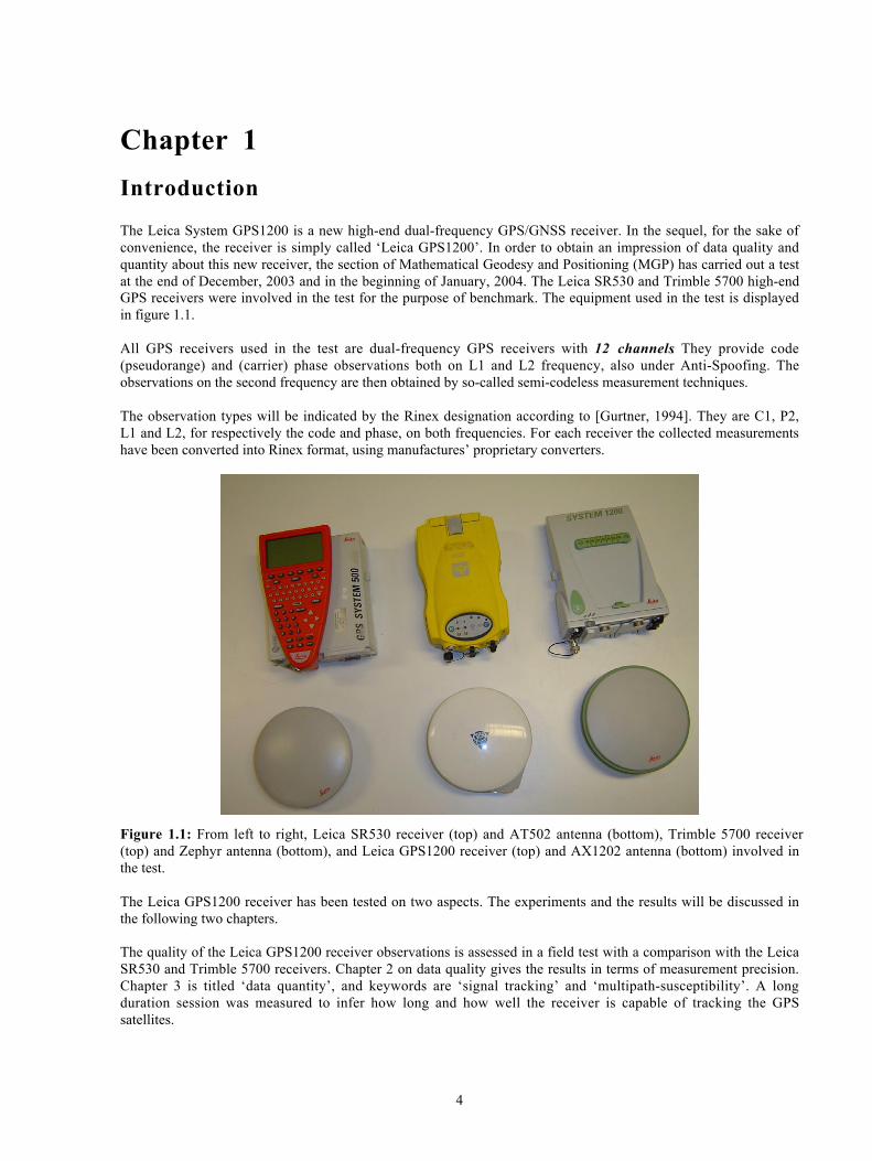
The Leica System GPS1200 is a new high-end dual-frequency GPS/GNSS receiver. In the sequel, for the sake ofconvenience, the receiver is simply called �Leica GPS1200�. In order to obtain an impression of data quality andquantity about this new receiver, the section of Mathematical Geodesy and Positioning (MGP) has carried out a testat the end of December, 2003 and in the beginning of January, 2004. The Leica SR530 and Trimble 5700 high-endGPS receivers were involved in the test for the purpose of benchmark. The equipment used in the test is displayedin figure 1.1.
All GPS receivers used in the test are dual-frequency GPS receivers with 12 channels. They provide code(pseudorange) and (carrier) phase observations both on L1 and L2 frequency, also under Anti-Spoofing. Theobservations on the second frequency are then obtained by so-called semi-codeless measurement techniques.
The observation types will be indicated by the Rinex designation according to [Gurtner, 1994]. They are C1, P2,L1 and L2, for respectively the code and phase, on both frequencies. For each receiver the collected measurementshave been converted into Rinex format, using manufactures� proprietary converters.
Figure 1.1: From left to right, Leica SR530 receiver (top) and AT502 antenna (bottom), Trimble 5700 receiver(top) and Zephyr antenna (bottom), and Leica GPS1200 receiver (top) and AX1202 antenna (bottom) involved inthe test.
The Leica GPS1200 receiver has been tested on two aspects. The experiments and the results will be discussed inthe following two chapters.
The quality of the Leica GPS1200 receiver observations is assessed in a field test with a comparison with the LeicaSR530 and Trimble 5700 receivers. Chapter 2 on data quality gives the results in terms of measurement precision.Chapter 3 is titled �data quantity�, and keywords are �signal tracking� and �multipath-susceptibility�. A longduration session was measured to infer how long and how well the receiver is capable of tracking the GPSsatellites.
5
Chapter 2
Data Quality
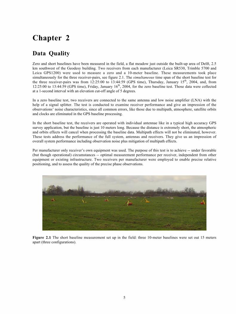
Zero and short baselines have been measured in the field, a flat meadow just outside the built-up area of Delft, 2.5km southwest of the Geodesy building. Two receivers from each manufacturer (Leica SR530, Trimble 5700 andLeica GPS1200) were used to measure a zero and a 10-meter baseline. These measurements took placesimultaneously for the three receiver-pairs, see figure 2.1. The simultaneous time span of the short baseline test forthe three receiver-pairs was from 12:25:00 to 13:44:59 (GPS time), Thursday, January 15th, 2004, and, from12:25:00 to 13:44:59 (GPS time), Friday, January 16th, 2004, for the zero baseline test. Those data were collectedat a 1-second interval with an elevation cut-off angle of 5 degrees.
In a zero baseline test, two receivers are connected to the same antenna and low noise amplifier (LNA) with thehelp of a signal splitter. The test is conducted to examine receiver performance and give an impression of theobservations� noise characteristics, since all common errors, like those due to multipath, atmosphere, satellite orbitsand clocks are eliminated in the GPS baseline processing.
In the short baseline test, the receivers are operated with individual antennae like in a typical high accuracy GPSsurvey application, but the baseline is just 10 meters long. Because the distance is extremely short, the atmosphericand orbits effects will cancel when processing the baseline data. Multipath effects will not be eliminated, however.These tests address the performance of the full system, antennas and receivers. They give us an impression ofoverall system performance including observation noise plus mitigation of multipath effects.
Per manufacturer only receiver�s own equipment was used. The purpose of this test is to achieve -- under favorable(but though operational) circumstances -- optimal measurement performance per receiver, independent from otherequipment or existing infrastructure. Two receivers per manufacturer were employed to enable precise relativepositioning, and to assess the quality of the precise phase observations.
Figure 2.1: The short baseline measurement set up in the field: three 10-meter baselines were set out 15 metersapart (three configurations).
6
2.1 Baseline Processing
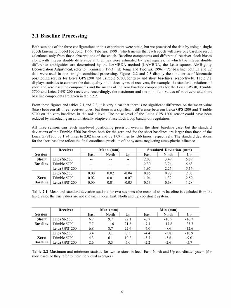
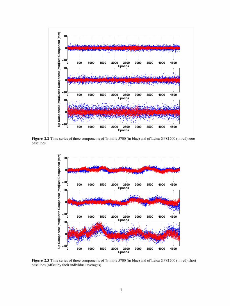
Both sessions of the three configurations in this experiment were static, but we processed the data by using a singleepoch kinematic model [de Jong, 1999; Tiberius, 1999], which means that each epoch will have one baseline resultcalculated only from those observations of the epoch. Baseline components and differential receiver clock biasesalong with integer double difference ambiguities were estimated by least squares, in which the integer doubledifference ambiguities are determined by the LAMBDA method (LAMBDA, the Least-squares AMBiguityDecorrelation Adjustment, refer to [Teunissen, 1993], [de Jonge and Tiberius, 1996]). Per baseline, both L1 and L2data were used in one straight combined processing. Figures 2.2 and 2.3 display the time series of kinematicpositioning results for Leica GPS1200 and Trimble 5700, for zero and short baselines, respectively. Table 2.1displays statistics to compare the data quality of all three types of receivers, for example, the standard deviations ofshort and zero baseline components and the means of the zero baseline components for the Leica SR530, Trimble5700 and Leica GPS1200 receivers. Accordingly, the maximum and the minimum values of both zero and shortbaseline components are given in table 2.2.
From these figures and tables 2.1 and 2.2, it is very clear that there is no significant difference on the mean value(bias) between all three receiver types, but there is a significant difference between Leica GPS1200 and Trimble5700 on the zero baselines in the noise level. The noise level of the Leica GPS 1200 sensor could have beenreduced by introducing an automatically adaptive Phase Lock Loop bandwidth regulation.
All three sensors can reach mm-level positioning precision even in the short baseline case, but the standarddeviations of the Trimble 5700 baselines both for the zero and for the short baselines are larger than those of theLeica GPS1200 by 1.94 times to 2.02 times and by 1.09 times to 1.66 times, respectively. The standard deviationsfor the short baseline reflect the final coordinate precision of the systems neglecting atmospheric influences.
Mean (mm) Standard Deviation (mm)Session
ReceiverEast North Up East North Up
Leica SR530 -- -- -- 2.03 3.49 5.89Trimble 5700 -- -- -- 2.30 3.74 5.63
ShortBaseline
Leica GPS1200 -- -- -- 1.97 2.25 5.16Leica SR530 0.00 0.02 -0.04 0.86 0.98 2.03Trimble 5700 0.02 0.01 0.07 1.04 1.32 2.59Zero
Baseline Leica GPS1200 0.00 0.01 -0.05 0.53 0.68 1.28
Table 2.1: Mean and standard deviation statistic for two sessions (the mean of short baseline is excluded from thetable, since the true values are not known) in local East, North and Up coordinate system.
Max (mm) Min (mm)Session
ReceiverEast North Up East North Up
Leica SR530 6.7 9.7 22.1 -6.7 -10.5 -16.7Trimble 5700 7.7 11.6 21.8 -7.4 -17.8 -23.7
ShortBaseline
Leica GPS1200 6.8 8.7 22.6 -7.0 -8.6 -12.6Leica SR530 3.4 3.1 8.5 -4.4 -3.8 -10.9Trimble 5700 4.3 6.1 10.2 -3.7 -5.6 -9.0Zero
Baseline Leica GPS1200 2.6 3.3 5.0 -2.2 -2.6 -5.7
Table 2.2: Maximum and minimum statistic for two sessions in local East, North and Up coordinate system (forshort baseline they refer to their individual averages).
7
0 500 1000 1500 2000 2500 3000 3500 4000 4500−10
0
10
Epochs
Eas
t C
om
po
nen
t (m
m)
0 500 1000 1500 2000 2500 3000 3500 4000 4500−10
0
10
Epochs
No
rth
Co
mp
on
ent
(mm
)
0 500 1000 1500 2000 2500 3000 3500 4000 4500−10
0
10
Epochs
Up
Co
mp
on
ent
(mm
)
Figure 2.2: Time series of three components of Trimble 5700 (in blue) and of Leica GPS1200 (in red) zerobaselines.
0 500 1000 1500 2000 2500 3000 3500 4000 4500−20
0
20
Epochs
Eas
t C
om
po
nen
t (m
m)
0 500 1000 1500 2000 2500 3000 3500 4000 4500−20
0
20
Epochs
No
rth
Co
mp
on
ent
(mm
)
0 500 1000 1500 2000 2500 3000 3500 4000 4500−20
0
20
Epochs
Up
Co
mp
on
ent
(mm
)
Figure 2.3: Time series of three components of Trimble 5700 (in blue) and of Leica GPS1200 (in red) shortbaselines (offset by their individual averages).
8
2.2 Least-Squares Residuals
For the processing of the residuals, in-house software, namely the RELRES program, was used [de Jong, 1999].The processing of the data is done epoch-by-epoch. We will analyze the least-squares single difference residualsof the adjustments. Under the working mathematical model, the residuals of the single difference observations areexpected to have zero mean. The residuals represent the measurements noise and they show biases and anomalieswhen present. A similar analysis was made in [Bona and Tiberius, 2000]. Note that in our analysis the a-prioristandard deviation of the least-squares residual is constant and the same for all epochs and all channels (satellites),so that time-series of residuals later on can be mutually compared.
In discussing the figures 2.4 through 2.11 we consider biases, trends and variations in the time series, and, apartfrom these, we make an attempt to quantify the width of the noise band, in order to present an indication on thenominal receiver noise. Before doing so, we address the issue of time correction. It should be kept in mindthroughout this chapter, that in general, filtering or smoothing brings down the noise level, at the price of timecorrelation. Additionally, multipath in the short baseline may introduce time-correlation to the observations.
9
0 1000 2000 3000 4000−20
−10
0
10
20
Res
idu
al [
mm
]
Time [s]
Zero Baseline, Leica SR530, PRN21, L1
0 1000 2000 3000 4000−20
−10
0
10
20
Res
idu
al [
mm
]
Time [s]
Zero Baseline, Leica SR530, PRN10, L1
0 1000 2000 3000 4000−20
−10
0
10
20
Res
idu
al [
mm
]
Time [s]
Zero Baseline, Leica GPS1200, PRN21, L1
0 1000 2000 3000 4000−20
−10
0
10
20
Res
idu
al [
mm
]
Time [s]
Zero Baseline, Leica GPS1200, PRN10, L1
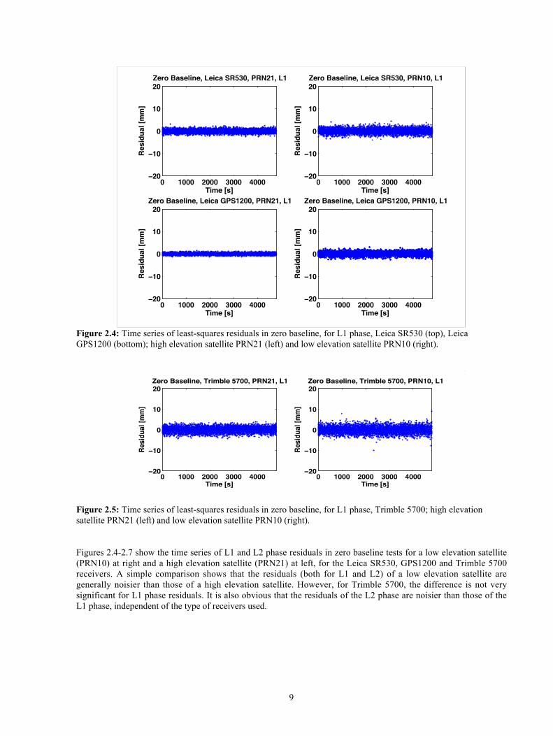
Figure 2.4: Time series of least-squares residuals in zero baseline, for L1 phase, Leica SR530 (top), LeicaGPS1200 (bottom); high elevation satellite PRN21 (left) and low elevation satellite PRN10 (right).
0 1000 2000 3000 4000−20
−10
0
10
20
Res
idua
l [m
m]
Time [s]
Zero Baseline, Trimble 5700, PRN21, L1
0 1000 2000 3000 4000−20
−10
0
10
20
Res
idua
l [m
m]
Time [s]
Zero Baseline, Trimble 5700, PRN10, L1
Figure 2.5: Time series of least-squares residuals in zero baseline, for L1 phase, Trimble 5700; high elevationsatellite PRN21 (left) and low elevation satellite PRN10 (right).
Figures 2.4-2.7 show the time series of L1 and L2 phase residuals in zero baseline tests for a low elevation satellite(PRN10) at right and a high elevation satellite (PRN21) at left, for the Leica SR530, GPS1200 and Trimble 5700receivers. A simple comparison shows that the residuals (both for L1 and L2) of a low elevation satellite aregenerally noisier than those of a high elevation satellite. However, for Trimble 5700, the difference is not verysignificant for L1 phase residuals. It is also obvious that the residuals of the L2 phase are noisier than those of theL1 phase, independent of the type of receivers used.
10
0 1000 2000 3000 4000−20
−10
0
10
20
Res
idu
al [
mm
]
Time [s]
Zero Baseline, Leica SR530, PRN21, L2
0 1000 2000 3000 4000−20
−10
0
10
20
Res
idu
al [
mm
]
Time [s]
Zero Baseline, Leica SR530, PRN10, L2
0 1000 2000 3000 4000−20
−10
0
10
20
Res
idu
al [
mm
]
Time [s]
Zero Baseline, Leica GPS1200, PRN21, L2
0 1000 2000 3000 4000−20
−10
0
10
20
Res
idu
al [
mm
]
Time [s]
Zero Baseline, Leica 1200, PRN10, L2
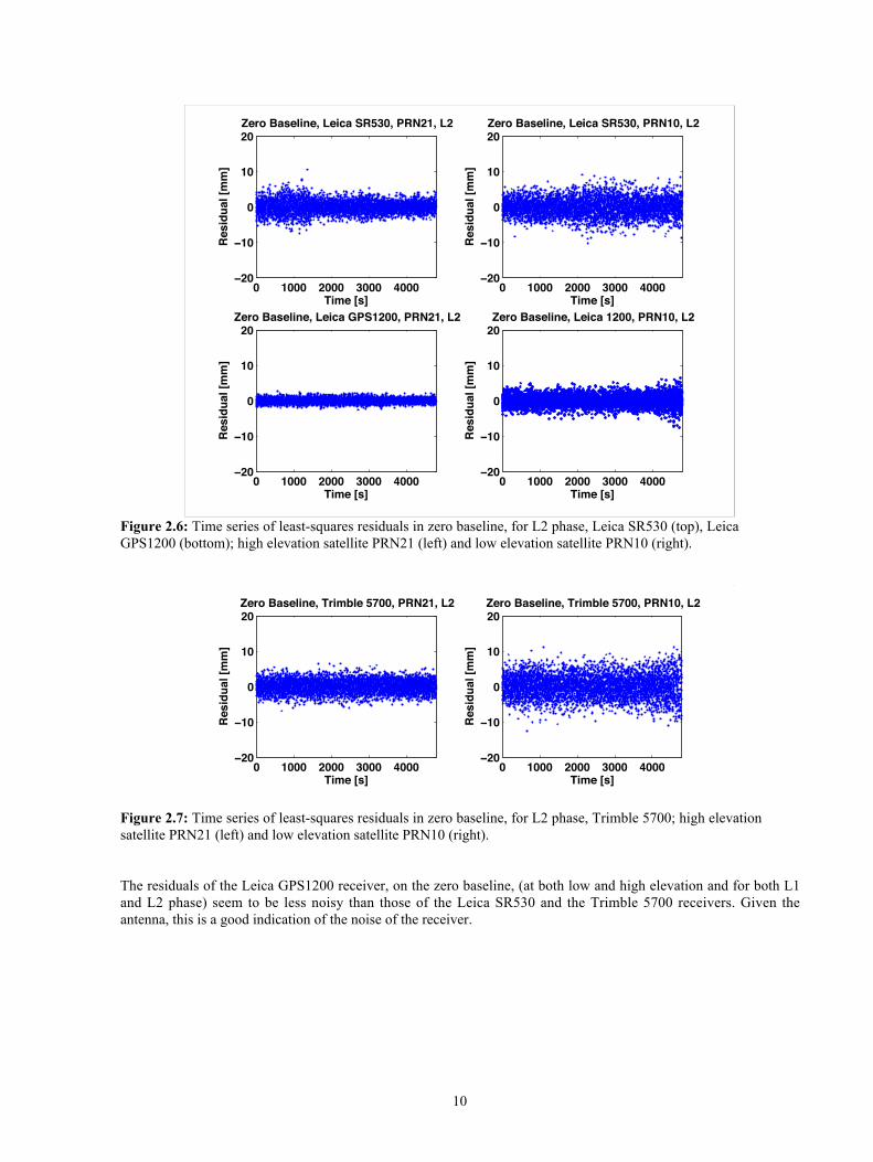
Figure 2.6: Time series of least-squares residuals in zero baseline, for L2 phase, Leica SR530 (top), LeicaGPS1200 (bottom); high elevation satellite PRN21 (left) and low elevation satellite PRN10 (right).
0 1000 2000 3000 4000−20
−10
0
10
20
Res
idu
al [
mm
]
Time [s]
Zero Baseline, Trimble 5700, PRN21, L2
0 1000 2000 3000 4000−20
−10
0
10
20
Res
idu
al [
mm
]
Time [s]
Zero Baseline, Trimble 5700, PRN10, L2
Figure 2.7: Time series of least-squares residuals in zero baseline, for L2 phase, Trimble 5700; high elevationsatellite PRN21 (left) and low elevation satellite PRN10 (right).
The residuals of the Leica GPS1200 receiver, on the zero baseline, (at both low and high elevation and for both L1and L2 phase) seem to be less noisy than those of the Leica SR530 and the Trimble 5700 receivers. Given theantenna, this is a good indication of the noise of the receiver.
11
0 1000 2000 3000 4000−100
−50
0
50
100
Res
idu
al [
cm]
Time [s]
Zero Baseline, Leica SR530, PRN21, C1
0 1000 2000 3000 4000−100
−50
0
50
100
Res
idu
al [
cm]
Time [s]
Zero Baseline, Leica SR530, PRN10, C1
0 1000 2000 3000 4000−100
−50
0
50
100
Res
idu
al [
cm]
Time [s]
Zero Baseline, Leica GPS1200, PRN21, C1
0 1000 2000 3000 4000−100
−50
0
50
100
Res
idu
al [
cm]
Time [s]
Zero Baseline, Leica GPS1200, PRN10, C1
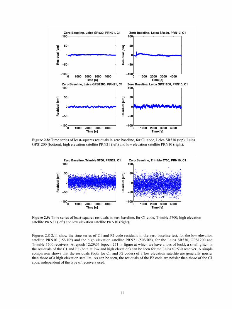
Figure 2.8: Time series of least-squares residuals in zero baseline, for C1 code, Leica SR530 (top), LeicaGPS1200 (bottom); high elevation satellite PRN21 (left) and low elevation satellite PRN10 (right).
0 1000 2000 3000 4000−100
−50
0
50
100
Res
idu
al [
cm]
Time [s]
Zero Baseline, Trimble 5700, PRN21, C1
0 1000 2000 3000 4000−100
−50
0
50
100
Res
idu
al [
cm]
Time [s]
Zero Baseline, Trimble 5700, PRN10, C1
Figure 2.9: Time series of least-squares residuals in zero baseline, for C1 code, Trimble 5700; high elevationsatellite PRN21 (left) and low elevation satellite PRN10 (right).
Figures 2.8-2.11 show the time series of C1 and P2 code residuals in the zero baseline test, for the low elevationsatellite PRN10 (15º-10º) and the high elevation satellite PRN21 (50º-70º), for the Leica SR530, GPS1200 andTrimble 5700 receivers. At epoch 12:29:31 (epoch 271 in figure at which we have a loss of lock), a small glitch inthe residuals of the C1 and P2 (both at low and high elevation) can be seen for the Leica SR530 receiver. A simplecomparison shows that the residuals (both for C1 and P2 codes) of a low elevation satellite are generally noisierthan those of a high elevation satellite. As can be seen, the residuals of the P2 code are noisier than those of the C1code, independent of the type of receivers used.
12
0 1000 2000 3000 4000−100
−50
0
50
100
Res
idu
al [
cm]
Time [s]
Zero Baseline, Leica SR530, PRN21, P2
0 1000 2000 3000 4000−100
−50
0
50
100
Res
idu
al [
cm]
Time [s]
Zero Baseline, Leica SR530, PRN10, P2
0 1000 2000 3000 4000−100
−50
0
50
100
Res
idu
al [
cm]
Time [s]
Zero Baseline, Leica GPS1200, PRN21, P2
0 1000 2000 3000 4000−100
−50
0
50
100
Res
idu
al [
cm]
Time [s]
Zero Baseline, Leica GPS1200, PRN10, P2
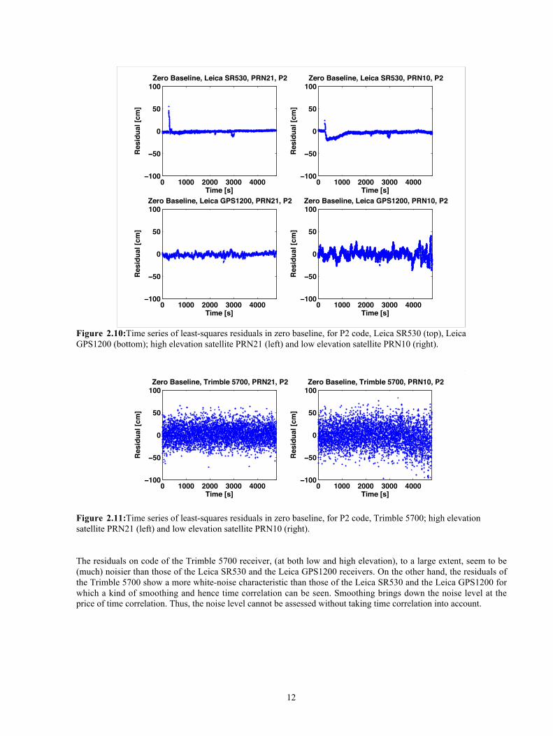
Figure 2.10: Time series of least-squares residuals in zero baseline, for P2 code, Leica SR530 (top), LeicaGPS1200 (bottom); high elevation satellite PRN21 (left) and low elevation satellite PRN10 (right).
0 1000 2000 3000 4000−100
−50
0
50
100
Res
idu
al [
cm]
Time [s]
Zero Baseline, Trimble 5700, PRN21, P2
0 1000 2000 3000 4000−100
−50
0
50
100
Res
idu
al [
cm]
Time [s]
Zero Baseline, Trimble 5700, PRN10, P2
Figure 2.11: Time series of least-squares residuals in zero baseline, for P2 code, Trimble 5700; high elevationsatellite PRN21 (left) and low elevation satellite PRN10 (right).
The residuals on code of the Trimble 5700 receiver, (at both low and high elevation), to a large extent, seem to be(much) noisier than those of the Leica SR530 and the Leica GPS1200 receivers. On the other hand, the residuals ofthe Trimble 5700 show a more white-noise characteristic than those of the Leica SR530 and the Leica GPS1200 forwhich a kind of smoothing and hence time correlation can be seen. Smoothing brings down the noise level at theprice of time correlation. Thus, the noise level cannot be assessed without taking time correlation into account.

13
Table 2.3 : Standard deviation (std), maximum (max) and minimum (min) values of residuals (L1, L2 C1 and P2)for a high (PRN21) and a low (PRN10) elevation satellite, zero baseline, all in millimeters.
Satellite PRN21 Satellite PRN10Type Receiver Std.
(mm)Max.(mm)
Min.(mm)
Std. (mm)
Max.(mm)
Min.(mm)
Leica SR530 2.4 9.3 -8.1 8.5 25.4 -21.8Trimble 5700 2.2 8.4 -7.4 8.2 28.4 -18.4L1Leica GPS1200 2.2 8.4 -5.6 7.3 32.6 -22.2Leica SR530 3.7 15.1 -10.8 12.2 36.5 -25.9Trimble 5700 2.8 7.8 -11.5 10.5 34.7 -32.5L2Leica GPS1200 3.3 8.1 -9.4 9.4 23.3 -27Leica SR530 44 54 -227 174 496 -372Trimble 5700 241 927 -971 402 1550 -1544C1Leica GPS1200 64 179 -229 144 405 -608Leica SR530 114 183 -296 250 670 -298Trimble 5700 272 1031 -1334 406 1172 -1849P2Leica GPS1200 80 359 -308 245 1392 -676
Table 2.4 : Standard deviation (std), maximum (max) and minimum (min) values of residuals (L1, L2, C1 and P2)for a high (PRN21) and a low (PRN10) elevation satellite, short baseline, all in millimeters.
The tables 2.3 and 2.4 present the minimum and maximum value of the least-squares residuals over the full 1 hour20 minutes period, for a high elevation satellite (PRN21) and a low elevation satellite (PRN10), for eachobservation type. Also the standard deviation is given.
From figures 2.4 to 2.11, we can obtain some comparative impressions not only on the Leica SR530, LeicaGPS1200 and the Trimble 5700 receivers, but also different behavior on high elevation and low elevation satellites.These figures allow us to see the details, from which we can conclude at least:
Satellite PRN21 Satellite PRN10Type Receiver Std.
(mm)Max.(mm)
Min.(mm)
Std.(mm)
Max.(mm)
Min.(mm)
Leica SR530 0.7 3.2 -2.4 1 4.5 -3.9Trimble 5700 1.3 3.8 -4.3 1.6 8.9 -9.9L1Leica GPS1200 0.4 1.4 -1.4 0.7 3.0 -2.6Leica SR530 1.8 10.5 -7.5 2.5 9.2 -10.2Trimble 5700 1.8 6.6 -6.8 3.2 11.1 -12.6L2Leica GPS1200 0.7 2.7 -2.5 1.6 6.4 -7.6Leica SR530 14 56 -92 36 168 -105Trimble 5700 154 697 -546 255 808 -1076C1Leica GPS1200 23 56 -85 44 134 -151Leica SR530 31 552 -127 51 237 -221Trimble 5700 188 656 -714 246 831 -1299P2Leica GPS1200 37 101 -196 95 395 -370
14
1) The residuals of a high elevation satellite are generally less noisy than those of a low elevation satellite nomatter which type of receivers, however, this conclusion is not very distinct in the case of the zerobaseline. The reason has been given in the beginning of this chapter.
2) The residuals of the L1 phase observations are less noisy when compared to those of the L2 phase.3) The residuals of the L1 and L2 phase for the Leica GPS1200 receiver seem to be less noisy than those of
the Leica SR530 and Trimble 5700 receivers both on the short baseline and the zero baseline.
Further numerical values for statistics on the residuals as mean, median and standard deviation per satellite (andhence elevation) are presented in section 2.4.
2.3 Time-Correlation of Phase Residuals
Here we will investigate the common assumption with data processing, of observations possessing only whitenoise. That is, they are not correlated from epoch to epoch. We consider a correlogram of the time-series of theleast-squares residual. The correlogram gives the auto-correlation coefficient versus lag (the interval between twosamples). The coefficient at lag 0 equals 1 by definition. If the residual would be a white noise process, then allother coefficients should be about zero, otherwise, the residuals probably show the behavior of time correlation.Two aspects may cause time-correlation for the least-squares residuals: one is that the observations are quite noisy(e.g. because of the anti-spoofing encryption) so that some smoothing or filtering may be applied, while, the otherone is that some time-correlation error resources, such as multipath effects, atmospheric delays, remain in theresiduals after data processing. The latter (external) cause can generally be ruled out on zero baseline data.
15
0 10 20 30 40 50−0.5
0
0.5
1 Zero Baseline, Leica SR530, PRN21, L1
Lags [s]
Co
rrel
atio
n
0 10 20 30 40 50−0.5
0
0.5
1 Zero Baseline, Leica SR530, PRN10, L1
Lags [s]
Co
rrel
atio
n
0 10 20 30 40 50−0.5
0
0.5
1 Zero Baseline, Leica GPS1200, PRN21, L1
Lags [s]
Co
rrel
atio
n
0 10 20 30 40 50−0.5
0
0.5
1 Zero Baseline, Leica GPS1200, PRN10, L1
Lags [s]
Co
rrel
atio
n
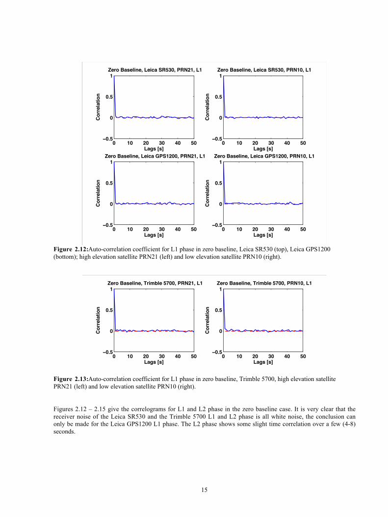
Figure 2.12: Auto-correlation coefficient for L1 phase in zero baseline, Leica SR530 (top), Leica GPS1200(bottom); high elevation satellite PRN21 (left) and low elevation satellite PRN10 (right).
0 10 20 30 40 50−0.5
0
0.5
1 Zero Baseline, Trimble 5700, PRN21, L1
Lags [s]
Co
rrel
atio
n
0 10 20 30 40 50−0.5
0
0.5
1 Zero Baseline, Trimble 5700, PRN10, L1
Lags [s]
Co
rrel
atio
n
Figure 2.13: Auto-correlation coefficient for L1 phase in zero baseline, Trimble 5700, high elevation satellitePRN21 (left) and low elevation satellite PRN10 (right).
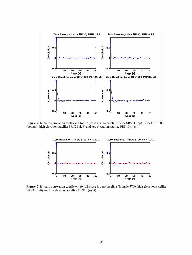
Figures 2.12 � 2.15 give the correlograms for L1 and L2 phase in the zero baseline case. It is very clear that thereceiver noise of the Leica SR530 and the Trimble 5700 L1 and L2 phase is all white noise, the conclusion canonly be made for the Leica GPS1200 L1 phase. The L2 phase shows some slight time correlation over a few (4-8)seconds.
16
0 10 20 30 40 50−0.5
0
0.5
1 Zero Baseline, Leica SR530, PRN21, L2
Lags [s]
Co
rrel
atio
n
0 10 20 30 40 50−0.5
0
0.5
1 Zero Baseline, Leica SR530, PRN10, L2
Lags [s]
Co
rrel
atio
n
0 10 20 30 40 50−0.5
0
0.5
1 Zero Baseline, Leica GPS1200, PRN21, L2
Lags [s]
Co
rrel
atio
n
0 10 20 30 40 50−0.5
0
0.5
1 Zero Baseline, Leica GPS1200, PRN10, L2
Lags [s]
Co
rrel
atio
n
Figure 2.14: Auto-correlation coefficient for L2 phase in zero baseline, Leica SR530 (top), Leica GPS1200(bottom); high elevation satellite PRN21 (left) and low elevation satellite PRN10 (right).
0 10 20 30 40 50−0.5
0
0.5
1 Zero Baseline, Trimble 5700, PRN21, L2
Lags [s]
Co
rrel
atio
n
0 10 20 30 40 50−0.5
0
0.5
1 Zero Baseline, Trimble 5700, PRN10, L2
Lags [s]
Co
rrel
atio
n
Figure 2.15: Auto-correlation coefficient for L2 phase in zero baseline, Trimble 5700, high elevation satellitePRN21 (left) and low elevation satellite PRN10 (right).
17
2.4 Residual Statistics
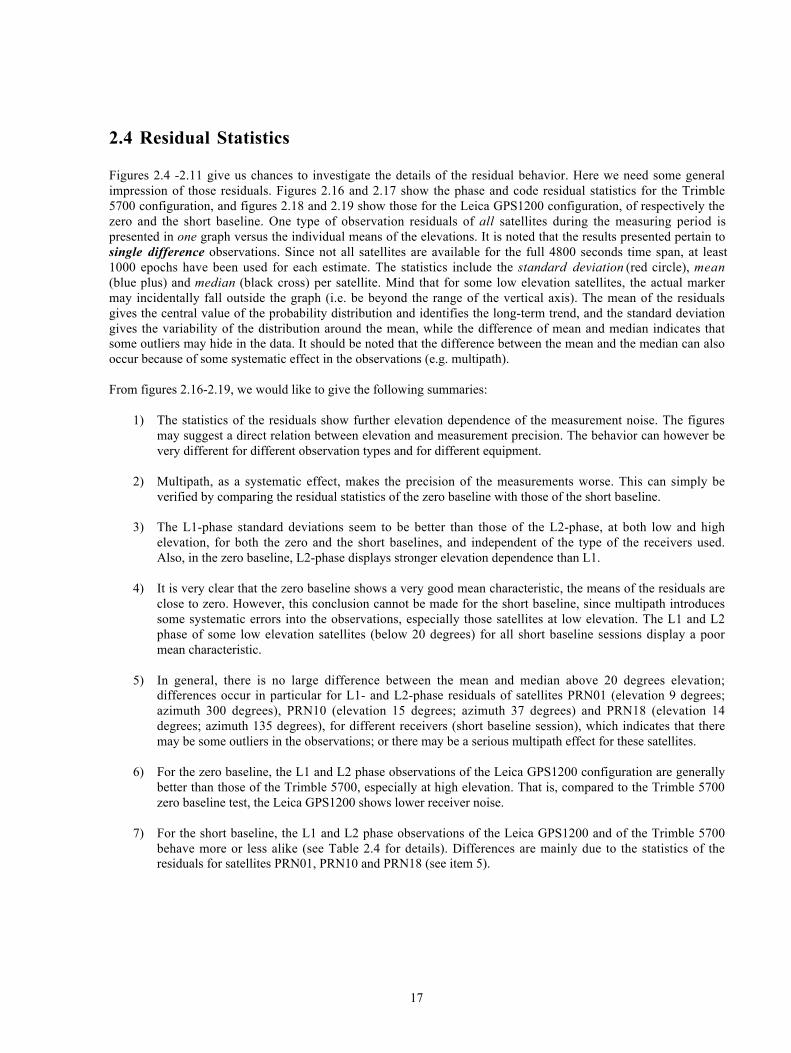
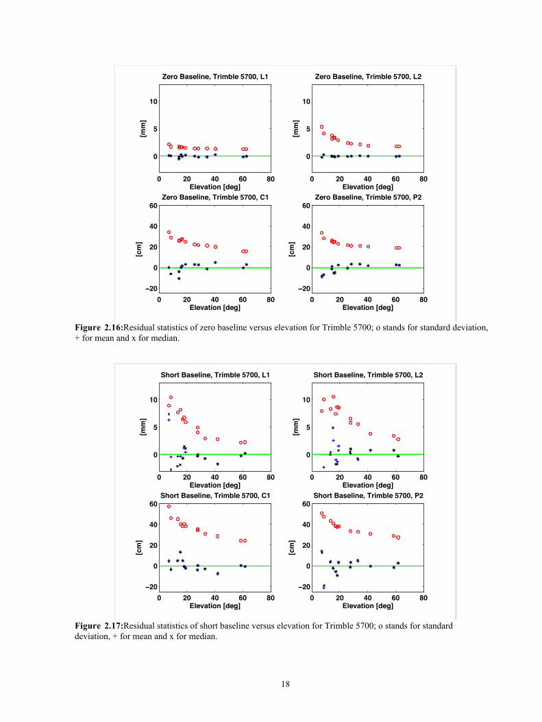
Figures 2.4 -2.11 give us chances to investigate the details of the residual behavior. Here we need some generalimpression of those residuals. Figures 2.16 and 2.17 show the phase and code residual statistics for the Trimble5700 configuration, and figures 2.18 and 2.19 show those for the Leica GPS1200 configuration, of respectively thezero and the short baseline. One type of observation residuals of all satellites during the measuring period ispresented in one graph versus the individual means of the elevations. It is noted that the results presented pertain tosingle difference observations. Since not all satellites are available for the full 4800 seconds time span, at least1000 epochs have been used for each estimate. The statistics include the standard deviation (red circle), mean(blue plus) and median (black cross) per satellite. Mind that for some low elevation satellites, the actual markermay incidentally fall outside the graph (i.e. be beyond the range of the vertical axis). The mean of the residualsgives the central value of the probability distribution and identifies the long-term trend, and the standard deviationgives the variability of the distribution around the mean, while the difference of mean and median indicates thatsome outliers may hide in the data. It should be noted that the difference between the mean and the median can alsooccur because of some systematic effect in the observations (e.g. multipath).
From figures 2.16-2.19, we would like to give the following summaries:
1) The statistics of the residuals show further elevation dependence of the measurement noise. The figuresmay suggest a direct relation between elevation and measurement precision. The behavior can however bevery different for different observation types and for different equipment.
2) Multipath, as a systematic effect, makes the precision of the measurements worse. This can simply beverified by comparing the residual statistics of the zero baseline with those of the short baseline.
3) The L1-phase standard deviations seem to be better than those of the L2-phase, at both low and highelevation, for both the zero and the short baselines, and independent of the type of the receivers used.Also, in the zero baseline, L2-phase displays stronger elevation dependence than L1.
4) It is very clear that the zero baseline shows a very good mean characteristic, the means of the residuals areclose to zero. However, this conclusion cannot be made for the short baseline, since multipath introducessome systematic errors into the observations, especially those satellites at low elevation. The L1 and L2phase of some low elevation satellites (below 20 degrees) for all short baseline sessions display a poormean characteristic.
5) In general, there is no large difference between the mean and median above 20 degrees elevation;differences occur in particular for L1- and L2-phase residuals of satellites PRN01 (elevation 9 degrees;azimuth 300 degrees), PRN10 (elevation 15 degrees; azimuth 37 degrees) and PRN18 (elevation 14degrees; azimuth 135 degrees), for different receivers (short baseline session), which indicates that theremay be some outliers in the observations; or there may be a serious multipath effect for these satellites.
6) For the zero baseline, the L1 and L2 phase observations of the Leica GPS1200 configuration are generallybetter than those of the Trimble 5700, especially at high elevation. That is, compared to the Trimble 5700zero baseline test, the Leica GPS1200 shows lower receiver noise.
7) For the short baseline, the L1 and L2 phase observations of the Leica GPS1200 and of the Trimble 5700behave more or less alike (see Table 2.4 for details). Differences are mainly due to the statistics of theresiduals for satellites PRN01, PRN10 and PRN18 (see item 5).
18
0 20 40 60 80
0
5
10
[mm
]
Elevation [deg]
Zero Baseline, Trimble 5700, L1
0 20 40 60 80
0
5
10
[mm
]
Elevation [deg]
Zero Baseline, Trimble 5700, L2
0 20 40 60 80
−20
0
20
40
60
[cm
]
Elevation [deg]
Zero Baseline, Trimble 5700, C1
0 20 40 60 80
−20
0
20
40
60
[cm
]
Elevation [deg]
Zero Baseline, Trimble 5700, P2
Figure 2.16: Residual statistics of zero baseline versus elevation for Trimble 5700; o stands for standard deviation,+ for mean and x for median.
0 20 40 60 80
0
5
10
[mm
]
Elevation [deg]
Short Baseline, Trimble 5700, L1
0 20 40 60 80
0
5
10
[mm
]
Elevation [deg]
Short Baseline, Trimble 5700, L2
0 20 40 60 80
−20
0
20
40
60
[cm
]
Elevation [deg]
Short Baseline, Trimble 5700, C1
0 20 40 60 80
−20
0
20
40
60
[cm
]
Elevation [deg]
Short Baseline, Trimble 5700, P2
Figure 2.17: Residual statistics of short baseline versus elevation for Trimble 5700; o stands for standarddeviation, + for mean and x for median.

19
0 20 40 60 80
0
5
10
[mm
]
Elevation [deg]
Zero Baseline, Leica GPS1200, L1
0 20 40 60 80
0
5
10
[mm
]
Elevation [deg]
Zero Baseline, Leica GPS1200, L2
0 20 40 60 80
−20
0
20
40
60
[cm
]
Elevation [deg]
Zero Baseline, Leica GPS1200, C1
0 20 40 60 80
−20
0
20
40
60
[cm
]
Elevation [deg]
Zero Baseline, Leica GPS1200, P2
Figure 2.18: Residual statistics of zero baseline versus elevation for Leica GPS1200; o stands for standarddeviation, + for mean and x for median.
0 20 40 60 80
0
5
10
[mm
]
Elevation [deg]
Short Baseline, Leica GPS1200, L1
0 20 40 60 80
0
5
10
[mm
]
Elevation [deg]
Short Baseline, Leica GPS1200, L2
0 20 40 60 80
−20
0
20
40
60
[cm
]
Elevation [deg]
Short Baseline, Leica GPS1200, C1
0 20 40 60 80
−20
0
20
40
60
[cm
]
Elevation [deg]
Short Baseline, Leica GPS1200, P2
Figure 2.19: Residual statistics of short baseline versus elevation for Leica GPS1200; o stands for standarddeviation, + for mean and x for median.
20
We have investigated the details of the residual behavior, the estimated statistics of observations per satellite andthe time-correlation of the observation residuals as well. Here we focus on the non-diagonal elements of the singledifference observations� variance-covariance, the covariances between different GPS observation types. From thevariances and covariances, one can compute the empirical correlation coefficient, which can explore the cross-correlation relationship between different GPS observation types [Tiberius and Kenselaar, 2003]. To be allowed touse only one single variance value for all channels / satellites, we here restrict our computations to the residuals ofonly two satellites PRN21 and PRN16, both with elevations larger than 45° in the case of the zero baseline.
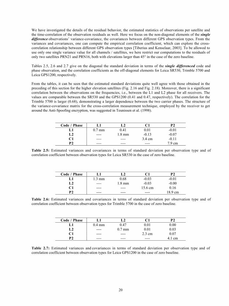
Tables 2.5, 2.6 and 2.7 give on the diagonal the standard deviation in terms of the single differenced code andphase observation, and the correlation coefficients as the off-diagonal elements for Leica SR530, Trimble 5700 andLeica GPS1200, respectively.
From the tables, it can be seen that the estimated standard deviations quite well agree with those obtained in thepreceding of this section for the higher elevation satellites (Fig. 2.16 and Fig. 2.18). Moreover, there is a significantcorrelation between the observations on the frequencies, i.e., between the L1 and L2 phase for all receivers. Thevalues are comparable between the SR530 and the GPS1200 (0.41 and 0.47, respectively). The correlation for theTrimble 5700 is larger (0.68), demonstrating a larger dependence between the two carrier phases. The structure ofthe variance-covariance matrix for the cross-correlation measurement technique, employed by the receiver to getaround the Anti-Spoofing encryption, was suggested in Teunissen et al. (1998).
Table 2.5: Estimated variances and covariances in terms of standard deviation per observation type and ofcorrelation coefficient between observation types for Leica SR530 in the case of zero baseline.
Table 2.6: Estimated variances and covariances in terms of standard deviation per observation type and ofcorrelation coefficient between observation types for Trimble 5700 in the case of zero baseline.
Table 2.7: Estimated variances and covariances in terms of standard deviation per observation type and ofcorrelation coefficient between observation types for Leica GPS1200 in the case of zero baseline.
Code / Phase L1 L2 C1 P2L1 0.7 mm 0.41 0.01 -0.01L2 ---- 1.8 mm -0.13 -0.07C1 ---- ---- 3.4 cm -0.11P2 ---- ---- ---- 7.9 cm
Code / Phase L1 L2 C1 P2L1 1.3 mm 0.68 -0.03 -0.01L2 ---- 1.8 mm -0.03 -0.00C1 ---- ---- 15.6 cm 0.16P2 ---- ---- ---- 18.9 cm
Code / Phase L1 L2 C1 P2L1 0.4 mm 0.47 0.01 0.00L2 ---- 0.7 mm 0.01 0.03C1 ---- ---- 2.3 cm 0.07P2 ---- ---- ---- 4.1 cm
21
Chapter 3
Data Quantity
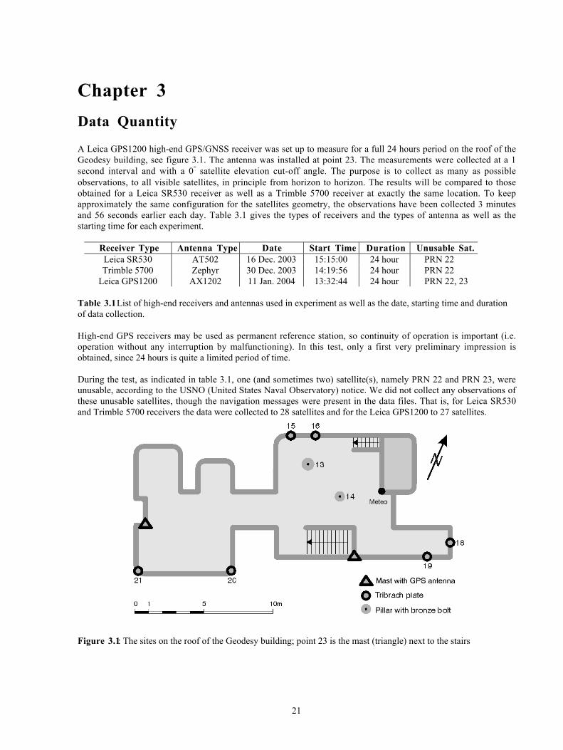
A Leica GPS1200 high-end GPS/GNSS receiver was set up to measure for a full 24 hours period on the roof of theGeodesy building, see figure 3.1. The antenna was installed at point 23. The measurements were collected at a 1second interval and with a 0° satellite elevation cut-off angle. The purpose is to collect as many as possibleobservations, to all visible satellites, in principle from horizon to horizon. The results will be compared to thoseobtained for a Leica SR530 receiver as well as a Trimble 5700 receiver at exactly the same location. To keepapproximately the same configuration for the satellites geometry, the observations have been collected 3 minutesand 56 seconds earlier each day. Table 3.1 gives the types of receivers and the types of antenna as well as thestarting time for each experiment.
Receiver Type Antenna Type Date Start Time Duration Unusable Sat.Leica SR530 AT502 16 Dec. 2003 15:15:00 24 hour PRN 22Trimble 5700 Zephyr 30 Dec. 2003 14:19:56 24 hour PRN 22
Leica GPS1200 AX1202 11 Jan. 2004 13:32:44 24 hour PRN 22, 23
Table 3.1 List of high-end receivers and antennas used in experiment as well as the date, starting time and durationof data collection.
High-end GPS receivers may be used as permanent reference station, so continuity of operation is important (i.e.operation without any interruption by malfunctioning). In this test, only a first very preliminary impression isobtained, since 24 hours is quite a limited period of time.
During the test, as indicated in table 3.1, one (and sometimes two) satellite(s), namely PRN 22 and PRN 23, wereunusable, according to the USNO (United States Naval Observatory) notice. We did not collect any observations ofthese unusable satellites, though the navigation messages were present in the data files. That is, for Leica SR530and Trimble 5700 receivers the data were collected to 28 satellites and for the Leica GPS1200 to 27 satellites.
Figure 3.1: The sites on the roof of the Geodesy building; point 23 is the mast (triangle) next to the stairs

22
3.1 Integrity Monitoring
The 24-hour data are processed and analysed with the integrity monitoring software [de Jong, 1997] developed atthe Department. Data analysis is possible on the observations of a single receiver to a single satellite. The integritymonitoring software aims at detecting in real-time outliers and slips in dual frequency data. For the presentanalysis, a post-processing version of the software is used.
The integrity monitoring software can provide the following statistics per satellite
counts of the number of complete observation epochsan epoch is complete if all code (C1 and P2) and phase (L1 and L2) observations to a satellite areavailable
counts of the number of incomplete observation epochsan epoch is incomplete if some or all of the code and phase observations to a satellite are missing(or when a full observation epoch is missing)
counts of the number of outliers in the C1 and P2 code observationstheoretically the software is able to detect outliers of approximately 4 times the a-priori codestandard deviation, which is fixed at 0.75 m
counts of the number of slips in the L1 and L2 phase observationstheoretically the software is able to detect slips of even 1 cycle
estimates of the standard deviation of the C1 and P2 code observationsthe standard deviations are estimated from linear combinations of code and phase observations
The linear combinations, Mc1 and Mp2, of observations read
21
21
11
11 LLCM C ααα
−−
−++=
21
11
1
222 LLPM P α
αα
α−+−
−+=
with 22
21 ff=α the ratio of the two GPS carrier frequencies, squared, and all observations C1, P2, L1 and L2
have been expressed in meters.
The geometric range to the satellite, the atmospheric delays and the clock errors are absent in these combinations.Present are the carrier phase ambiguities (of L1 and L2), but they are constants. These so-called multipathcombinations are free from time-varying effects and should thus be constants, apart from noise on the observations.The noise of the code (pseudorange) will thereby dominate. The combinations Mc1 and Mp2 give an impression ofthe measurement precision of the code (C1 or P2) and possibly of multipath effects.
In the sequel, three analyses are performed, based on the statistics provided by the integrity monitoring software:counts of observation epochs, and of outliers and slips
code standard deviation, as function of elevation
code standard deviation, as function of elevation and azimuth
23
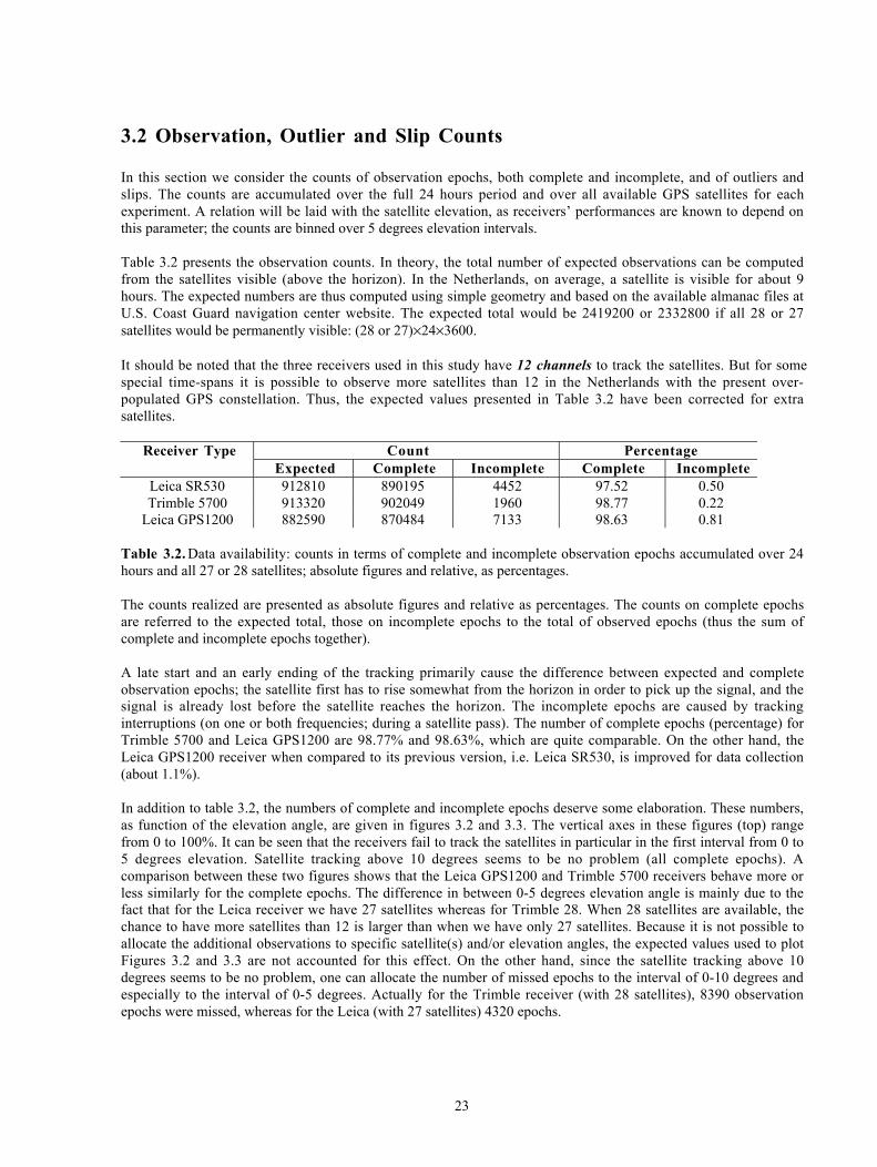
3.2 Observation, Outlier and Slip Counts
In this section we consider the counts of observation epochs, both complete and incomplete, and of outliers andslips. The counts are accumulated over the full 24 hours period and over all available GPS satellites for eachexperiment. A relation will be laid with the satellite elevation, as receivers� performances are known to depend onthis parameter; the counts are binned over 5 degrees elevation intervals.
Table 3.2 presents the observation counts. In theory, the total number of expected observations can be computedfrom the satellites visible (above the horizon). In the Netherlands, on average, a satellite is visible for about 9hours. The expected numbers are thus computed using simple geometry and based on the available almanac files atU.S. Coast Guard navigation center website. The expected total would be 2419200 or 2332800 if all 28 or 27satellites would be permanently visible: (28 or 27)×24×3600.
It should be noted that the three receivers used in this study have 12 channels to track the satellites. But for somespecial time-spans it is possible to observe more satellites than 12 in the Netherlands with the present over-populated GPS constellation. Thus, the expected values presented in Table 3.2 have been corrected for extrasatellites.
Count PercentageReceiver TypeExpected Complete Incomplete Complete Incomplete
Leica SR530 912810 890195 4452 97.52 0.50Trimble 5700 913320 902049 1960 98.77 0.22
Leica GPS1200 882590 870484 7133 98.63 0.81
Table 3.2. Data availability: counts in terms of complete and incomplete observation epochs accumulated over 24hours and all 27 or 28 satellites; absolute figures and relative, as percentages.
The counts realized are presented as absolute figures and relative as percentages. The counts on complete epochsare referred to the expected total, those on incomplete epochs to the total of observed epochs (thus the sum ofcomplete and incomplete epochs together).
A late start and an early ending of the tracking primarily cause the difference between expected and completeobservation epochs; the satellite first has to rise somewhat from the horizon in order to pick up the signal, and thesignal is already lost before the satellite reaches the horizon. The incomplete epochs are caused by trackinginterruptions (on one or both frequencies; during a satellite pass). The number of complete epochs (percentage) forTrimble 5700 and Leica GPS1200 are 98.77% and 98.63%, which are quite comparable. On the other hand, theLeica GPS1200 receiver when compared to its previous version, i.e. Leica SR530, is improved for data collection(about 1.1%).
In addition to table 3.2, the numbers of complete and incomplete epochs deserve some elaboration. These numbers,as function of the elevation angle, are given in figures 3.2 and 3.3. The vertical axes in these figures (top) rangefrom 0 to 100%. It can be seen that the receivers fail to track the satellites in particular in the first interval from 0 to5 degrees elevation. Satellite tracking above 10 degrees seems to be no problem (all complete epochs). Acomparison between these two figures shows that the Leica GPS1200 and Trimble 5700 receivers behave more orless similarly for the complete epochs. The difference in between 0-5 degrees elevation angle is mainly due to thefact that for the Leica receiver we have 27 satellites whereas for Trimble 28. When 28 satellites are available, thechance to have more satellites than 12 is larger than when we have only 27 satellites. Because it is not possible toallocate the additional observations to specific satellite(s) and/or elevation angles, the expected values used to plotFigures 3.2 and 3.3 are not accounted for this effect. On the other hand, since the satellite tracking above 10degrees seems to be no problem, one can allocate the number of missed epochs to the interval of 0-10 degrees andespecially to the interval of 0-5 degrees. Actually for the Trimble receiver (with 28 satellites), 8390 observationepochs were missed, whereas for the Leica (with 27 satellites) 4320 epochs.
24
The graphs at bottom on incomplete epochs reveal some data loss at low elevations. Note that the vertical axesrange here from 0 to 10%, so the rate of incomplete data is rather small. The incomplete epochs are caused at lowelevation angles (mainly between 0-5 degrees). A comparison between Figures 3.2 and 3.3 shows that the Trimble5700 and the Leica GPS1200 receivers lose approximately 2% and 5% of the data (as incomplete ones) in the 0-5degrees elevation angle interval. Since the total number of complete epochs for both receivers in this interval looksthe same, this may mean that the total number of observed (both complete and incomplete) epochs for the Leicareceiver is larger than for the Trimble receiver. This can also be verified from the results presented in Table 3.2.
Tables 3.3 and 3.4 give the number of outliers, for the C1 and P2 code observations with a 0 degree and 10 degreessatellite elevation cut-off angle, respectively. As can be seen from table 3.3, the outlier percentages of codeobservations, in general, are quite low. The C1 code has approximately 1000 outliers, which is negligible. A littlebit larger number for the P2 code is explained by the fact that the a-priori standard deviation for the code was set to0.75 m, and the P2 code shows a somewhat larger standard deviation at low elevation, which can also be seen fromfigures 3.4 and 3.5. Table 3.4 implies that most of the outliers (perhaps more than 90%) on C1 and P2 code happenin the low elevation range (0-10 degrees). However, this conclusion is not very distinct on P2 code for Trimble5700.
Tables 3.5 and 3.6 present the number of slips, for both the L1 and L2 phase observations with a 0-degree and 10-degrees satellite elevation cut-off angle, respectively. As can be seen from table 3.5, the number of L1 cycle slipsalmost equals the number of L2 cycle slips; it turns out that cycle slips on L1 and L2 occur usually simultaneouslywith these receivers. In general the number of cycle slips is rather limited. Table 3.6 implies that most of the slipson L1 and L2 phase happens in the low elevation range (0-10 degrees).
The numbers of outliers and slips under the header �percentage� both in table 3.3 and table 3.5 have beenreferenced each time to the number of complete epochs (in table 3.2). For tables 3.4 and 3.6, the number ofcomplete epochs has been adapted to reflect the 10-degrees elevation cut-off angle. The number of completeepochs for Trimble 5700 and Leica GPS1200 is 689977 and 662052. It should be concluded that with larger dataavailability (i.e., in particular at low elevation) outlier and slips become more likely to occur.
Count PercentageReceiver TypeC1 Code P2 Code C1 Code P2 Code
Trimble 5700 1141 2293 0.126 0.254Leica GPS1200 981 3365 0.113 0.387
Table 3.3: Outlier counts on C1 and P2 code, absolute figures and relative, as percentages of the number ofcomplete epochs, with 0 degree elevation cut-off angle.
Count PercentageReceiver TypeC1 Code P2 Code C1 Code P2 Code
Trimble 5700 99 1230 0.014 0.178Leica GPS1200 142 114 0.021 0.017
Table 3.4 Outlier counts on C1 and P2 code, absolute figures and relative, as percentages of the number ofcomplete epochs, with 10 degrees elevation cut-off angle.

25
0 10 20 30 40 50 60 70 80 900
20
40
60
80
100
Elevation of satellites (5 deg interval)
Per
cent
Number of complete epochs as % number of expected epochs
0 10 20 30 40 50 60 70 80 900
2
4
6
8
10
Elevation of satellites (5 deg interval)
Per
cent
Number of incomplete epochs as % number of observed epochs
Figure 3.2: Data collection by receiver Trimble 5700; number of complete epochs as percentage of the number ofexpected epochs, binned after elevation (top); number of incomplete epochs as percentage of the number ofobserved epochs, binned after elevation (bottom).
0 10 20 30 40 50 60 70 80 900
20
40
60
80
100
Elevation of satellites (5 deg interval)
Per
cent
Number of complete epochs as % number of expected epochs
0 10 20 30 40 50 60 70 80 900
2
4
6
8
10
Elevation of satellites (5 deg interval)
Per
cent
Number of incomplete epochs as % number of observed epochs
Figure 3.3: Data collection by receiver Leica GPS1200; number of complete epochs as percentage of the numberof expected epochs, binned after elevation (top); number of incomplete epochs as percentage of the number ofobserved epochs, binned after elevation (bottom).

26
Count PercentageReceiver TypeL1 Phase L2 Phase L1 Phase L2 Phase
Trimble 5700 2946 2876 0.327 0.319Leica GPS1200 2359 2430 0.271 0.279
Table 3.5: Slip counts on L1 and L2 phase, absolute figures and relative, as percentages of the complete epochs,with 0 degree elevation cut-off angle.
Count PercentageReceiver TypeL1 Phase L2 Phase L1 Phase L2 Phase
Trimble 5700 134 135 0.019 0.020Leica GPS1200 158 157 0.024 0.024
Table 3.6 Slip counts on L1 and L2 phase, absolute figures and relative, as percentages of the complete epochs,with 10 degrees elevation cut-off angle.
3.3 Code Standard Deviation
This section presents estimates of the standard deviation of the code observation (undifferenced), as function of thesatellite elevation. Observation noise is known to depend strongly on the satellite elevation. By the antenna gainpattern, the atmospheric path length and multipath, the quality of the observations will generally degrade withdecreasing elevation.
Figures 3.4 �and 3.5 give the estimates for the standard deviation of the C1 and P2 code observations of theTrimble 5700 and Leica GPS1200 receivers. The standard deviations for the code observations are computed for15 minutes time intervals, per satellite. They are plotted as a function of the elevation angle (mean value over the15 minutes period). The dependence of the noise on the satellite elevation is evident for all code observations. Andat the lowest elevation angles, the standard deviation estimates are, in most cases, suddenly smaller than that ofneighboring low elevation angles. This is probably related to the data loss below 5 degrees.
For the Trimble 5700 receiver, the standard deviation of multipath combinations for C1 and P2 code observationscomes down to 0.1-0.2 m at high elevations. For C1 code, it hardly exceeds 0.8 m at low elevation and it does notget better than 0.4 m. The general standard deviation estimated from all multipath combinations is 0.32 m. For P2code, the standard deviation of multipath combination hardly exceeds 1.1 m at low elevation and it does not getbetter than 0.3 m. The general standard deviation estimated from all multipath combinations is 0.33 m.

27
0 10 20 30 40 50 60 70 80 900
0.2
0.4
0.6
0.8
1
1.2
1.4
1.6
1.8
Elevation [deg]
Sta
ndar
d de
viat
ion
[m]
C1−code standard deviation estimates vs. elevation
Figure 3.4: Estimated standard deviation in meter for multipath combinations MC1 (left) and MP2 (right); Trimble5700 receiver.
0 10 20 30 40 50 60 70 80 900
0.2
0.4
0.6
0.8
1
1.2
1.4
1.6
1.8
Elevation [deg]
Sta
ndar
d de
viat
ion
[m]
C1−code standard deviation estimates vs. elevation
Figure 3.5: Estimated standard deviation in meter for multipath combinations MC1 (left) and MP2 (right); LeicaGPS1200 receiver.
For the Leica GPS1200, the standard deviation of multipath combinations for C1 and P2 code observations comesdown to 0.05 m at high elevations and it hardly exceeds 1.2 m at low elevation. It can get better than 0.2 m and 0.3m at low elevation for C1 and P2, respectively. The general standard deviation estimated from all multipathcombinations is 0.17 m and 0.21 m for C1 and P2 code, respectively.
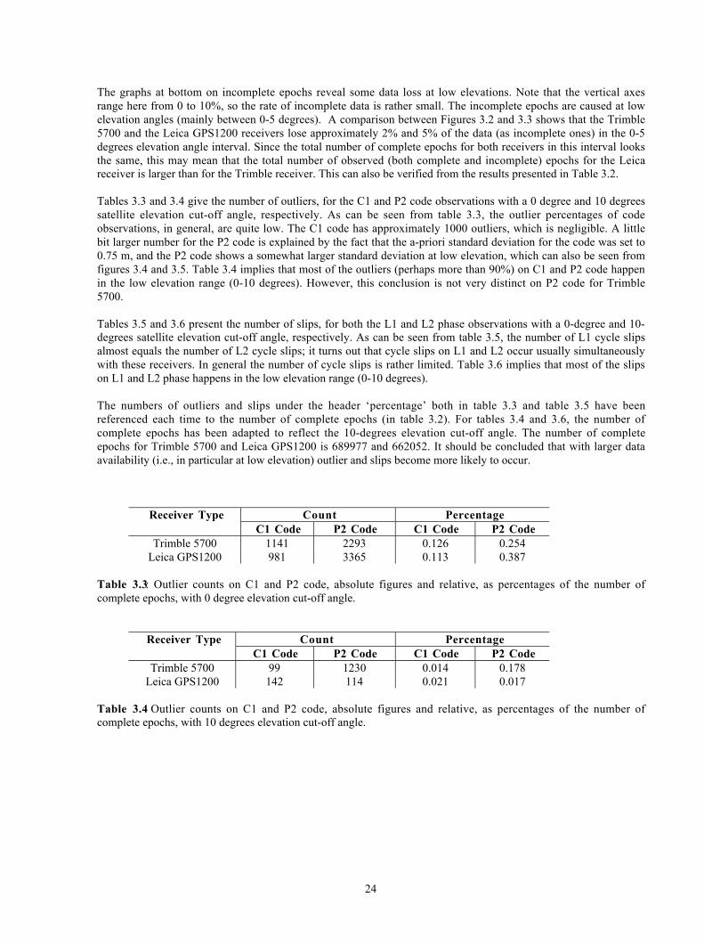
In the following we consider time series of the multipath combinations themselves. Figures 3.6 and 3.7 show themultipath combinations for one pass of satellite PRN 30. The horizontal axes represent 6 hours and 27 minutes.The solid green lines give the elevation angle, with the scale along the vertical axes at right. As can be seen fromthe figures, the C1 codes in blue are nearly as noisy as P2 codes in red for all receivers.
Figure 3.6 shows the multipath combinations for the Trimble 5700 receiver. The variation for both C1 and P2covers 2 m at low elevation, and just within 1 m at high elevation. As we mentioned before, the C1 and P2 codebehave similarly, however, the P2 code (in red) seems to be a little bit noisier than the C1 code (in green). Both ofthem, to some extent, are stable at the high elevation. The two multipath combinations give the impression that thetime series are more or less like a random series, which may imply independence of neighboring observations. Itseems that both receiver noise and multipath errors exist in this time series and the former plays the main role inthis combination.
0 10 20 30 40 50 60 70 80 900
0.2
0.4
0.6
0.8
1
1.2
1.4
1.6
1.8
Elevation [deg]
Sta
ndar
d de
viat
ion
[m]
P2−code standard deviation estimates vs. elevation
0 10 20 30 40 50 60 70 80 900
0.2
0.4
0.6
0.8
1
1.2
1.4
1.6
1.8
Elevation [deg]
Sta
ndar
d de
viat
ion
[m]
P2−code standard deviation estimates vs. elevation
28
Figure 3.7 shows the multipath combinations for the Leica GPS1200 receiver. The variation for both C1 and P2 iswithin 1 m at low elevation, and within 0.5 m at high elevation. The P2 code seems to be a little bit noisier than theC1 code. Both of them are quite stable at the high elevation. The time series of the multipath combination herecannot be interpreted as a random series from one sample to the next. A kind of smoothing and hence correlationbetween the observation epochs can be observed. As long as the receiver can bring down the noise level well, thiscorrelation can be expected because of multipath. That is, for the Leica receiver, it seems also that both receivernoise and multipath error exist in this multipath combination, but the latter plays the main role.
0 0.5 1 1.5 2
x 104
−6
−5
−4
−3
−2
−1
0
1
2
MP
2 [m
]
M
C1
[m]
Time [sec]
Multipath combination for a single pass satellite (c)
0 0.5 1 1.5 2
x 104
0
10
20
30
40
50
60
70
80
90
Ele
vatio
n an
gle
[deg
]
Figure 3.6. Multipath combinations MC1 (top, offset by the mean) and MP2 (bottom, offset by the mean withadding �3 m) as a function of time for a single pass of satellite PRN 30; Trimble 5700 receiver.
0 0.5 1 1.5 2
x 104
−6
−5
−4
−3
−2
−1
0
1
2
MP
2 [m
]
M
C1
[m]
Time [sec]
Multipath combination for a single pass satellite (a)
0 0.5 1 1.5 2
x 104
0
10
20
30
40
50
60
70
80
90
Ele
vatio
n an
gle
[deg
]
Figure 3.7. Multipath combinations MC1 (top, offset by the mean) and MP2 (bottom, offset by the mean withadding �3 m) as functions of time for a single pass of satellite PRN 30; Leica GPS1200 receiver.

29
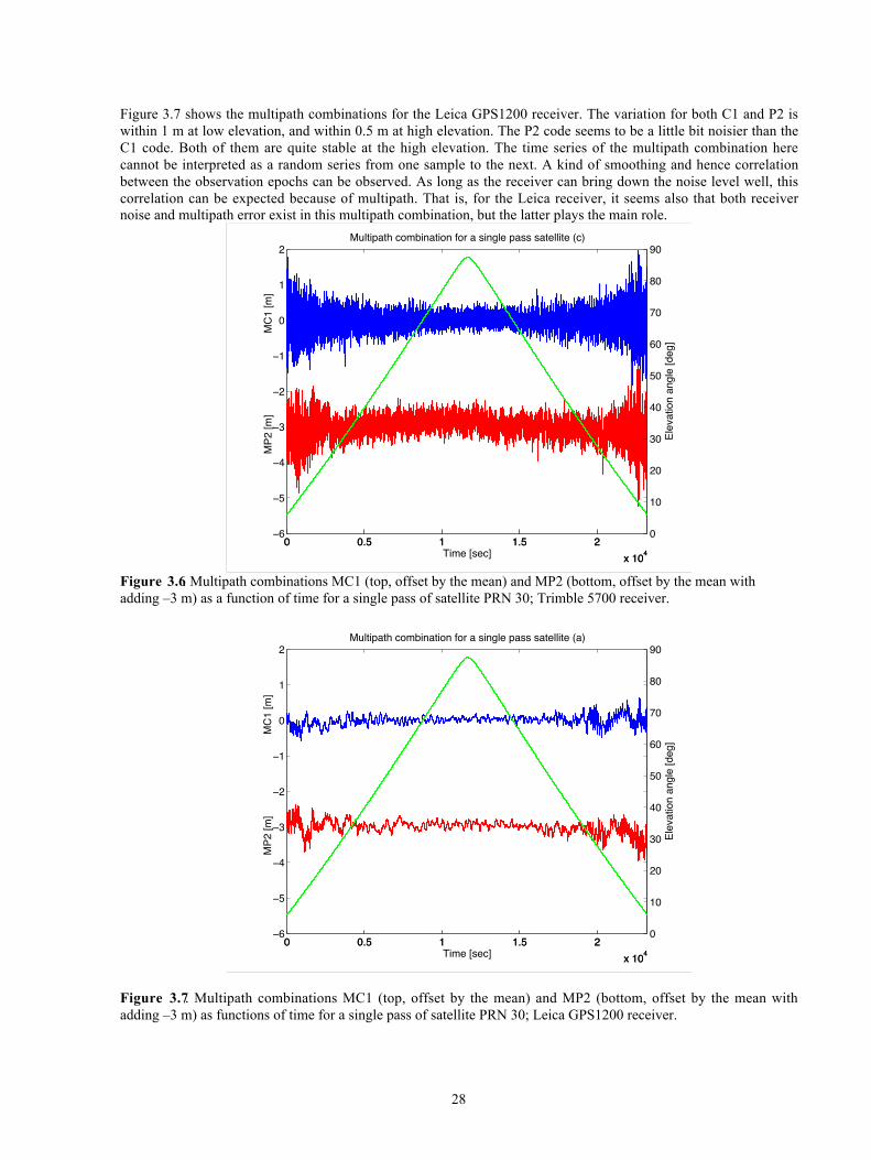
3.4 Standard Deviation Versus Elevation and Azimuth
Multipath effects depend on the receiver-satellite geometry. These effects may induce both an elevation andazimuth dependence on the statistics. The test location, point 23 on the mast is depicted in figure 3.8. Theobservation platform is to the left of this mast (mainly North). In figure 3.1 point 23 is the mast (triangle) in themiddle, next to the stairs.
In order to get an impression of the severity of the multipath conditions on the test location, standard deviations forthe code observations are computed for fixed 15 minutes time intervals and plot as a function of both satelliteazimuth and elevation, for C1 and P2 code observations for three experiments. In other words, we have plottedFigures 3.4 and 3.5 not only in terms of elevation angles but now also in terms of azimuth for each satellite.Figures 3.9 and 3.10 show the results. The same color bar, for both sky plots, has been used to make thecomparison simple. These graphs require careful inspection, as the differences are small.
If little or no multipath effects are present at a site, the estimates can be expected to be scattered more or lessrandom over the skyplot (at least for similar elevation angles). If, on the other hand, multipath is playing asignificant role, the best and worst estimates will show an uneven distribution, i.e. a dependence on azimuth. Thisis the case for both C1 and P2 code observations in Figures 3.9 and 3.10.
Figure 3.8: The AX1202 antenna on the top of the mast (point 23) on the roof of the Geodesy building;X = 3924693.553 m, Y = 301139.237 m, Z = 5001907.509 m (ITRF 2000 at epoch 2004.0).
The site is at 52 degrees latitude North.
30
03060
0
30
60
90
North
EastWest
South0
0.1
0.2
0.3
0.4
0.5
0.6
0.7
0.8
0.9
1
1.1
1.2
1.3
1.4
Figure 3.9: Code standard deviation estimates versus elevation and azimuth for C1 (left) and P2 (right).Trimble 5700 receiver.
03060
0
30
60
90
North
EastWest
South0
0.1
0.2
0.3
0.4
0.5
0.6
0.7
0.8
0.9
1
1.1
1.2
1.3
1.4
Figure 3.10: Code standard deviation estimates versus elevation and azimuth for C1 (left) and P2 (right);Leica GPS1200.
The worst estimates, the red, yellow, and probably green dots, are mainly concentrated in the North-East, i.e., thedirection to the roof of the observatory, see Figure 3.1. The North-West direction yields observations withrelatively less noise than that in the North-East direction. As such, the experiment turned out to be highlyrepeatable, and the azimuth-elevation multipath plots give a multipath �footprint� of the site on the Geodesybuilding. This analysis can serve as a multipath source locator.
For the Trimble 5700 receiver, Figure 3.9 shows the results. The worst estimates for both C1 and P2 areconcentrated in the North-East direction. In this direction, the standard deviation of C1 code seems to be a little bitbetter than that of P2 code. As can be seen, for both code observations, in general, the standard deviation estimatesget larger at low elevation.
For the Leica GPS1200 receiver, Figure 3.10 shows the results. The worst estimates for both C1 and P2 are againconcentrated in the North-East direction. In this direction, the standard deviation of C1 and P2 codes seems to bemore or less the same. As can be seen, for both code observations, in general, the standard deviation estimates donot get very much larger at low elevation (cf. Figure 3.9). That is, from this standpoint, at lower elevation angle,the Leica GPS1200 receiver has a better performance than the Trimble 5700 receiver.
03060
0
30
60
90
North
EastWest
South0
0.1
0.2
0.3
0.4
0.5
0.6
0.7
0.8
0.9
1
1.1
1.2
1.3
1.4
03060
0
30
60
90
North
EastWest
South0
0.1
0.2
0.3
0.4
0.5
0.6
0.7
0.8
0.9
1
1.1
1.2
1.3
1.4
31
Chapter 4
Summary and Conclusion
This report presents the results of the Leica GPS1200 receiver test carried out by the Mathematical Geodesy andPositioning (MGP) section in Delft in December, 2003 and January, 2004.
Chapter 2 gives an impression of the measurement performance in terms of measurement noise. The measurementswere collected out in the field under rather favorable, but realistic circumstances. By the constrained relativepositioning processing, the noise characteristics of both code and phase can be assessed. For the Leica GPS1200receiver, the precision of the phase observations is at the millimeter level, and for the code observations at thecentimeter-level. No severe biases were found in the range observations. From the results of single epoch precisepositioning, the standard deviation of the Leica GPS1200 baseline components turns out to be better than that forthe Leica SR530 and Trimble 5700 receivers, both for zero and short baseline. The L1 and L2 phase residuals forLeica GPS1200 receiver turn out to be less noisy than those for the Leica SR530 and Trimble 5700 receivers;though multipath effect behaves more or less alike for all receivers. The precision of the C1 and P2 codeobservations for Leica GPS1200 receiver turns out, to a large extent, to be better than that for the Trimble 5700receiver. However, the C1 and P2 code residuals of the Leica GPS1200 show time-correlation, while those for theTrimble 5700 show more or less a white-noise characteristic. That is, they are not correlated in time. Also, thecarrier phase observations on L1 and L2 are positively correlated for all receivers. The correlation for the Trimble5700 is larger than those for the Leica receivers.
Satellite tracking and multipath are dealt with in chapter 3. As a general rule, the receiver does follow a satelliteadequately from and again down to 10 degrees elevation. The results show that the Leica GPS1200 and Trimble5700 receivers behave more or less similarly for the number of complete epochs. But the number of observedepochs (both complete and incomplete) for the Leica GPS1200 receiver seems to be larger than for the Trimblereceiver. The general standard deviations estimated from all multipath combinations are 0.17 m for C1 code and0.21 m for P2 code (for Leica GPS1200) and 0.32 m for C1 code and 0.33 m for P2 code (for Trimble 5700),respectively.
As a conclusion, in general signal-tracking capability was found to be good. The receiver tested in the 24 hoursexperiment showed very few cycle slips in the phase observations and outliers in the code observations.Concerning high accuracy positioning the Leica GPS1200 receiver definitely represents the state-of-the-art intoday high-end GPS/GNSS receiver market.
32
Bibliography
[Bona and Tiberius, 2000] Bona, P. and Tiberius, C. (2000). An experimental comparison on noise characteristicof seven high-end dual frequency GPS receiver-sets. In Proceedings IEEE PLANS 2000 , pages 237-244. SanDiego, CA, USA, March 13-16.
[de Jong, 1997] de Jong, C. (1997). Principles and applications of permanent GPS arrays. PhD thesis, TUBudapest, Hungary.
[de Jong, 1999] de Jong, C. (1999). A modular approach to precise GPS positioning. GPS Solutions, Vol. 2, No. 4,pp. 52-56
[de Jonge and Tiberius, 1996] de Jonge, P. and Tiberius, C. (1996). The LAMBDA method for integer ambiguityestimation: implementation aspects. In: Delft Geodetic Computing Center LGR Series, No. 12, 45 pp.
[Gurtner, 1994] Gurtner, W. (1994). RINEX: Receiver Independent Exchange format. GPS World, 5(6): 48-52.Innovation Column.
[Liu, 2002] Liu, X. L. (2002). A comparison of stochastic models for GPS single differential kinematic positioning.In: Proceedings of ION GPS 2002, 24-27 September 2002, Portland, OR, pp. 1830-1841.
[Teunissen, 1993] Teunissen, P.J.G. (1993). Least-squares estimation of the integer GPS ambiguities. Invitedlectures, Section IV Theory and Methodology, IAG General Meeting, Beijing, China, August 1993. Also inDelft Geodetic Computing Center LGR Series, No.6, 16 pp.
[Teunissen et al, 1998] Teunissen, P.J.G., Tiberius, C.C.J.M., Jonkman, N.F., and de Jong, C.D. (1998).Consequences of the cross-correlation measurement technique. In: Proceedings GNSS98, CNES, Toulouse,France, 1-6
[Tiberius, 1999] Tiberius, C.C.J.M. (1999). The GPS data weight matrix: what are the issues? In: Proceedings ofNational Technical Meetings & 19th Biennal Guidance Test Symposium ION 1999, pp. 219-227, January 25-27, 1999 San Diego, CA
[Tiberius and Kenselaar, 2003] Tiberius, C. and Kenselaar, F. (2003). Variance component estimation and preciseGPS positioning: case study. Journal of Surveying Engineering, Vol. 129, No. 1, February 1, 2003

Leica Geosystems AGHeinrich-Wild-Strasse
CH-9435 Heerbrugg(Switzerland)
www.leica-geosystems.com Illustrations, descriptions and technical specifications are not binding and may change. Printed in Switzerland – Copyright Leica Geosystems AG, Heerbrugg, Switzerland, 2004. 741549 – V.04 – INT