GPU-friendly shape interpolation based on trajectory warping

SPECIAL ISSUE PAPER

GPU-friendly shape interpolation based ontrajectory warping

Lu Chen, Jin Huang, Hongxin Zhang and Wei Hua*

State Key Lab of CAD&CG, Zhejiang University 310058, Hangzhou, China

ABSTRACT

In this paper, we propose a GPU-friendly shape interpolation method. In contrast with state-of-the-art interpolation

algorithms, our method computes the trajectory of each vertex independently instead of solving large linear systems in

every interpolation step. Given two poses being interpolated, we find trajectory parameters for each vertex by optimization

with the consideration of the key pose reconstruction and as-rigid-as-possible deformation in the pre-computing stage.

During run-time, the vertices coordinates on the intermediate shape can be computed in parallel according to a close form

formulation. In the results we demonstrate that our method achieves extremely high performance on modern GPU and can

be extended easily to multi-pose interpolation. Copyright # 2011 John Wiley & Sons, Ltd.

KEYWORDS

shape interpolation; vertex path problem; trajectory warping

*Correspondence

Wei Hua, State Key Lab of CAD&CG, Zhejiang University 310058, Hangzhou, China.

E-mail: [email protected]

1. INTRODUCTION

Shape interpolation is a widely utilized technique in

computer animation, which interpolates between given

shapes to create attractive effects. In general, shape

interpolation includes two major issues: how to build a

one-to-one mapping between key shapes [1,2] and how to

compute trajectory between corresponding vertices during

the interpolation. In this paper, we focus on the latter issue,

i.e. the trajectory issue.

It is well-known that the explicit linear interpolation of

vertex coordinates suffers shrinkage problem, as illustrated

in Figure 1. To generate visual pleasant results, most of the

state-of-the-art methods [3–5] interpolate gradient infor-

mation or Laplacian coordinates instead of vertex

coordinates, and then implicitly reconstruct vertex coordi-

nates by optimizing least squares errors. Due to the as-

rigid-as-possible preserving nature of gradient domain

methods, such approaches can produce high quality shapes.

However, these methods need to solve large linear systems

in each interpolation step. The large amount memory

consumption of matrices makes them hard to interpolate

large models in realtime even with pre-computing step.

Moreover they are not GPU-friendly as vertex coordinates

cannot be reconstructed in a parallel way. Therefore,

gradient domain methods are not suitable for performance

demanding applications such as games and virtual reality.

In this paper, we propose an explicit nonlinearinterpolation method which can reconstruct the intermedi-

ate shape on GPUwithout shrinkage problem. The key idea

is to bring in a close form formulation of the vertex

trajectory for describing the interpolation procedure of

each vertex. Inspired by the modal-warping technique [6],

we regulate the linear interpolation trajectory with

additional angular velocity component for tracing the

local rotations. In this paper, we call this technique

trajectory warping, which can handle shape interpolation

properly even under large deformation cases.

The major contributions of our work include:

� A new close form interpolation trajectory which can

reconstruct the intermediate shape on GPU without

solving any equation.

� An optimization method to find the parameters of the

vertices trajectories which can interpolate given shapes

with as-rigid-as-possible energy constraints to avoid

producing interpolation artifacts.

2. RELATED WORK

As Ref. [7] provided a good survey of earlier work, we only

review several recent work related to 3D shape interp-

olation with feature preservation in this section.

COMPUTER ANIMATION AND VIRTUAL WORLDS

Comp. Anim. Virtual Worlds 2011; 22:285–294

Published online 12 April 2011 in Wiley Online Library (wileyonlinelibrary.com). DOI: 10.1002/cav.407

Copyright � 2011 John Wiley & Sons, Ltd. 285

Shape interpolation is related to feature preserving mesh

deformation [8–10]. These methods reconstruct deformed

shape according to given deformation gradient or

Laplacian coordinates by minimizing the changing of

local details. Most of these methods can be naturally

extended to shape interpolation [3,5,11] as the rotation

aspect of such local presentation can be easily separated

from the stretch and scale. By applying proper rotation

interpolation technique, intermediate shape can be

reconstructed according to interpolated deformation

gradient or Laplacian coordinates. All these gradient

domain methods produce high quality results but with the

cost of solving large linear systems.

Alternatively, literature [12] formulates the shape

interpolation problem as computing geodesic curves in

the shape space. Although their method can provide high

quality results, it is hard to generate intermediate shapes on

the fly unless by storing all the vertex positions for the

intermediate shapes.

To reduce the computational cost of gradient domain

methods, some other approaches adopt subspace tech-

nique. For example, Ref. [13] uses the methods proposed in

Ref. [14] to construct a generalized skeletal subspace. Ref.

[15] can compute the transformations for each bone

independently from the control points. To ensure the

deformation quality, they apply a Poisson-based solver.

With the help of the skeletal subspace, the dimensionality

of the linear system for reconstruction is greatly reduced. It

is worth mentioning that the recent work [16] also adopts

generalized skeletal structure for improving the interp-

olation quality with significant pose variation. However,

their method still requires solving a large linear system for

shape reconstruction.

Same as gradient domain methods, our method needs to

optimize shapes with as-rigid-as-possible deformation

constraints. However, this optimization is only occurred

in the pre-compute stage. During run-time, the trajectory of

each vertex is evaluated independently on the fly according

to trajectory warping. This is inspired by the modal

warping technique [6], which greatly improves the

traditional modal analysis to handle large rotation. In this

paper, we extend such a trajectory representation from

elastic object simulation into shape interpolation.

3. ALGORITHM

Given two consistent triangle meshes M0 and c with nvertices, the goal of shape interpolation is to find a

displacement trajectory function diðtÞ ðt2½0; 1�Þ for each

vertex xi. Let p0i and p

1i be positions of vertex xi onM0 and

M1, respectively. The interpolation trajectory of this

vertex can be expressed as:

piðtÞ ¼ p0i þ diðtÞ (1)

under position interpolation constraints:

dið0Þ ¼ 0 and p1i ¼ p0i þ dið1Þ (2)

In following sections, we will present a new close form

of trajectory diðtÞ for handling large rotation and introducean optimization strategy for finding the best trajectory of

each vertex.

3.1. Trajectory Warping

The most efficient trajectory calculation method is to use

linear interpolation of the vertex positions:

diðtÞ ¼ tðp1i�p0i Þ (3)

Figure 1. The pose interpolation results of armadillo model using linear interpolation (top) and our method (bottom), respectively. The

blue models in each row are the input poses.

286 Comp. Anim. Virtual Worlds 2011; 22:285–294 � 2011 John Wiley & Sons, Ltd.DOI: 10.1002/cav

GPU-friendly shape interpolation L. Chen et al.

Unfortunately, it cannot provide satisfied results under

large rotation as which involves high nonlinearity [7].

Based on this observation, the main idea of trajectory

warping is to introduce nonlinear correcting terms into the

trajectory formulation for compensating the rotation of

local frames.

As shown in Figure 2, the rotation can be achieved by

integrating the displacement velocity v(t) underrotational local frame as infinitesimal deformation.The displacement trajectory of a rotational vertex can bedescribed as below:

diðtÞ ¼Z t

0

RiðsÞviðsÞds (4)

where RiðtÞ is the rotation matrix representing the

orientation of the local frame. We employ Rodrigues

formula to express the rotation matrix in terms of the angle

uiðtÞ and the unit axis of rotation riðtÞ:RiðtÞ ¼ Iþ ½riðtÞ��sin uiðtÞð Þ

þ½riðtÞ�2� 1�cos uiðtÞð Þð Þ (5)

where ½ri�� denotes the standard skew symmetric matrix of

unit axis vector ri.During an interpolation procedure, steady and smooth

deformation of shapes are desired. So it is reasonable to

assume that the displacement velocity viðtÞ � vi and

riðtÞ � ri are constant, while uiðtÞ ¼ tui. Denote wiðtÞ ¼uiðtÞriðtÞ, then the displacement trajectory function can be

simplified:

diðtÞ ¼ t~Rðt;wiÞvi (6)

where

~Rðt;wiÞ ¼ Iþ ½ri�� 1�cosðtuiÞtui

þ½ri�2� 1� sinðtuiÞtui

� � (7)

In this simplification, wi and vi can be considered asthe per-vertex angular and displacement velocities,respectively. Compared with the linear interpolationtrajectory, wi introduces nonlinear warping which isessential for handling large rotation.

3.2. Velocity Optimization

With trajectory warping, our interpolation problem is

converted to finding the optimal angular and displacement

velocities for all the vertices. Let v and w be both 3n� 1vectors which pack the vi and wi of all the vertexpositions into column vectors. In our approach, tomake the trajectory start fromM0 and end withM1 aswell as keep the intermediate shapes as rigid as possible,velocities w and v are selected by minimizing thefollowing energy function:

Eðv;wÞ ¼ a2Epose þ b2Erot þ g2Egrad (8)

where a, b, and g are weights. In the objective function,

Epose and Erot are key pose and rotation energy terms,

respectively. For further controlling the shape qualities during

interpolation, we also introduce a gradient energy term Egrad.

Note that once we get the parameters of the vertex

trajectories, the intermediate shape vertex positions can be

calculated in parallel according to Equations (1) and (6) for

any interpolation parameter t.

3.2.1. Key Pose Energy.As the requirement of shape interpolation, the trajectory

must pass the target shape M1 at time t¼ 1. It implies the

following pose constraint energy must be minimized

Epose ¼ k~RðwÞv�ðP1�P0Þk2 (9)

where P0 and P1 are both 3n� 1 vectors standing forthe vertex coordinates of the interpolation shapes,and ~RðwÞ ¼ diagð~Rð1;w1Þ; . . . ; ~Rð1;wnÞÞ is a block-diagonal matrix.

Note that ~Rðt;wiÞ � ~Rð1; twiÞ, then we have ~RðtwÞ ¼diagð~Rðt;w1Þ; . . . ; ~Rðt;wnÞÞ, which will be used in the

following sections.

3.2.2. Rotation Energy.In our method, angular velocities w is used to representthe rotational variation of local frame. To keepinterpolation results as rigid as possible, w should beclose to the rotational variation caused by the localdisplacement velocity v for tracking the local frame well.Let v be per-vertex defined velocity field by viði ¼ 1; . . . ; nÞ. According to the kinematics of infini-tesimal deformation analysis [6], it shows that thefollowing least square on each vertex xi should beminimized:

kwi� 1

2r� vðxiÞk2 (10)

In Equation (10), symbol 5� stands for curl operation.12r� vðxiÞ is viewed as the rotational component of

velocity field v on vertex xi. Note that here we assume that

the curl operation is constant during all infinitesimal steps

of the deformation.

However, it is not trivial to calculate 12r� v on a

triangular mesh. Inspired by Ref. [17], we adopt following

approximation method to calculate per-vertex rotationalFigure 2. Local coordinate frames of rotational deformation.

Comp. Anim. Virtual Worlds 2011; 22:285–294 � 2011 John Wiley & Sons, Ltd.DOI: 10.1002/cav

287

L. Chen et al. GPU-friendly shape interpolation

component of the velocity field. Let A be a triangle which

undergoes a deformation and (p0i , vi) (i¼ 1, 2, 3)represents its three vertex positions in static state andlocal displacement velocities, respectively. Thenrotational variation of triangle A can be approximatedby a linear matrix product WAvA with

WA ¼ �K�1 ½q1�� j q2�� j ½q3��

vTA ¼ vT1 j vT2 j vT3� � (11)

where qi ¼ p0i� 13

Pi p

0i and K ¼ P3

i ½qi�2�.For the rotational component on a vertex, we use the

average of the rotational variation of all the triangles sharing

the same vertex. Thus, we could assemble the matrices WA

of all the triangles to form the global curlmatrixW, whichis in dimension 3n� 3n. Finally we obtain the rotationenergy on the total mesh as following:

Erot ¼ kw�Wvk2 (12)

3.2.3. Intermediate Gradient Energy.Notice that the global curl matrix W only restricts therotation component of the deformation. In many cases,the shape interpolation may involve a large degree ofstretching or compression. In such cases, the rotationcomponent is not dominant. If we only consider keypose and rotation energy, the resultant interpolationmay give rise to a sort of distortions. Figure 3 illustratesone such example. Hence we need to introduceadditional terms to control scaling and shearing duringinterpolation.

To overcome such problem, our solution is partly

inspired by Refs. [4,18]. We introduce an as-rigid-as-

possible deformation gradient to guide the shape interp-

olation. Consider a triangle A on shape M0 who is under

deformation and its vertex positions at time t are pti (i¼ 1,

2, 3). For calculating the deformation gradient of this

deforming triangle, we employ the surface-based defor-

mation gradient proposed in Ref. [19], which is equivalent

to the ‘‘volumetric’’ one [3] on the tetrahedron mesh but

does not involve a fourth vertex. Let ptA ¼ ðpt1jpt2jpt3Þ, thenthe surface-based deformation gradient of this triangle D

t

A

can be calculated by:

Dt

A ¼ ptAGA (13)

and

GA ¼1 0 0

0 1 0

�1 �1 0

0@

1A p01�p03jp02�p03jnA� ��1

(14)

where nA is the normal vector of the triangle inundeformed state and GA is the linear gradientoperator.

For the target interpolated deformation gradient,

considering the triangle A referred above, we first calculate

the transformation of this triangle from start to end DA

(3� 3), using method described in Ref. [3] whichinvolves the fourth vertices. Then, according to Ref. [4],we interpolate the rotational and scale/shear com-ponents of DA separately:

gtA ¼ RtAðtSAÞ (15)

where gtA is the as-rigid-as-possible interpolated defor-

mation gradient matrix at time t. RA and SA are obtainedby polar factorization DA ¼ RASA and Rt

A is therotational interpolation of RA with I.

Notice that the surface-based gradient Dt

A discards the

normal component [19] and for our intermediate gradient

constraint, the target interpolated gradients should also

Figure 3. The comparison of without (top)/with (bottom) the intermediate gradient energy control.



remove the degree of freedom along the normal direction:

gtA ¼ gtA�gtAnAnTA (16)

We use this as-rigid-as-possible deformation gradient as

a guidance constraint at the intermediate frame:

EgradtðAÞ ¼ kptAGA�gtAk2F (17)

In practice, we find that under the key pose and rotation

constraints, we can efficiently optimize the interpolation by

only constraining the deformation gradient of intermediate

frame t¼ 0.5.

Summarizing all the constraint energies on all mtriangles with repacking the gradient operator matrices and

target gradient vectors into 9m� 3n matrix G and 9m� 1vector g0:5, we can get the global form of gradientguidance constraint energy in terms of velocitiesparameters:

Egrad ¼XA

Egrad0:5ðAÞ

¼ kGP0:5�g0:5k2

¼ k 12G~R

w

2

� �v� g0:5�GP0

� �k2¼D k 1

2G~R

w

2

� �v�gk2

(18)

4. IMPLEMENTATION

In this section, we presents the implementation details on

solving the optimization problem of Equation (8) for

trajectory warping.

4.1. Gauss-Newton Algorithm

We adopt Gauss-Newton method to solve this optimization

problem. Note that the objective function is a sum of

squares, we can rewrite it in dot product form of vector F,i.e. Eðv;wÞ ¼ FTF. Moreover let J(v, w) be theJacobian matrix of vector F(v, w). Base on thisconfiguration, the whole optimization is performedin an iterative way:

vkþ1 ¼ vk þ dkvwkþ1 ¼ wk þ dkw

�(19)

where (dkv, dkw) is obtained by solving following linear least

squares problem

argmindkv ;d

kw

Jðvk;wkÞ dkvdkw

� �þ Fðvk;wkÞ

��2

(20)

4.2. Initial Value

To obtain the initial value (v0, w0), we first calculate thelocal frame variation of vertex xi by averaging rotation

components of its neighboring triangles N i:

w0i ¼

1

jN ijXAj2N i

logðRjÞ (21)

here Rj is the rotation component of the deformationgradient Dj of triangle Aj and extracted by polardecomposition Dj ¼ RjSj. When the shape defor-mation involves mainly the rotation component, theintegration of the rotation vector wi will be close to thevariation of local frame around this vertex. Thereforew0

i is a good estimation of per-vertex angular velocity.Hence we assemble all of them as the initial angularvelocity vector w0 in our solver.

The initial value of the displacement velocity is

calculated by:

v0 ¼ ~Rðw0Þ� ��1ðP1�P0Þ (22)

We find that under most cases, the nonlinear optimiz-

ations converge within 10 iterations by adopting these

initial values.

4.3. Weighting Schema

To select meaningful weights, we first calculate a base set

of weights a0, b0, and g0 such that Hessian matrices of

energy terms Epos, Erot, and Egrad have same Frobenius

norms. Then, because the pose constraint is expected to be a

hard constraint for our shape interpolation application, we set

the weight a¼ a0 as the largest weight in our optimization.

For the weights of the compatibility and intermediate

gradient constraints, we found that a large range of values

work well and a minimal amount of example-specific tuning

is required. In this paper, we use the setting of b ¼ 0:1 � b0

and g ¼ 0:05 � g0 for most of the examples.

4.4. Post-Processing

After solving the optimization, we can compute the

velocities (v, w) for performing the interpolation.However in the velocity optimization [Equation (8)],pose energy Epose acts as a soft constraint which cannotbe exactly ensure pose interpolation. Therefore we needto adopt a simple post-processing. That is we modifydisplacement velocities to directly satisfy the poseinterpolation constraint [Equation (2)]:

v0 ¼ ~RðwÞ� ��1ðP1�P0Þ: (23)

After this, we can ensure that the trajectories interpolate

shape M1 when t¼ 1. Usually the changes brought in by

the post-procedure can not be noticed visually because the

residuals are very small when the optimization converges.

5. RESULTS AND DISCUSSIONS

Our framework can be applied to various scenarios and

applications. In this section we will first show several


289


applications of our method. Then performance will be

reported as well. Finally, we will discuss an extension of

our trajectory warping technique for better handling an

intrinsic complex articulated motion.

5.1. Applications

5.1.1. Two Shapes Interpolation.Figure 1 shows pose interpolation between two armadillo

poses. Our method can handle the large deformations of the

legs. Figure 4 shows the morphing result between two head

models. The results of our method are as good as those of

Poisson Interpolation [5] and the comparisons between

Poisson method and ours can be found in the companion

video.

5.1.2. Multi-Pose Interpolation.Given K multiple poses Mk (k2f1; . . . ;Kg) and one

reference pose Mr, we can calculate the vector pairs

fvk;wkg for all poses. Consider the poses Mk as a pose

space refer to Mr , the vector pairs fvk;wkg could be

viewed as the coordinates of these poses in this high

dimension space. The multi-pose interpolation could be

transformed into interpolating the vector pairs. Given a set

of interpolation weights jk (k2f1; . . . ;Kg), the coordinatesof the interpolated pose is:

fvinter;winterg ¼XKk¼1

jkvk;XKk¼1

jkwk

( )(24)

and the new pose could be reconstructed in our framework

with Equation 6:

Pinter ¼ P0 þ ~RðwinterÞvinter (25)

Figure 5 shows the multi-pose interpolation between

armadillo poses. The top three poses are given and the first

one is used as the reference pose. The triangle areas with

red points indicate the interpolation weights. The three

corners correspond to the input poses and the weights are

(1, 0, 0), (0, 1, 0), and (0, 0, 1). The red point inside the

triangle area indicates the weight as its barycentric

Figure 4. The morphing result between head models.

Figure 5. Multi-pose interpolation between armadillo poses.



coordinate. The bottom four poses are interpolated using

the weights shown by the above triangle figures.

Because our reconstruction procedure is very fast, the

users can interactively change the weights and get the

interpolated shape in real-time. The effects of this real-time

multi-pose interpolation are demonstrated in the compa-

nion video. Users can create new animation interactively

by interpolating the existing poses in real-time.

5.2. Timing and Comparison

Table 1 shows the statistics of the demos in this paper,

including the complexity of the models and the perform-

ance of the algorithm. All the timings in the table are

measured on an Intel Pentium Dual 2.0GHz (only one core

used), 3.0GB RAM machine with a NVIDIA GForce

9800GT graphics card.

The third column in the table shows one iteration time of

our nonlinear optimization solver and the fourth column

shows the iteration times before the solver converges. The

fifth column shows the run-time interpolation performance

on GPU. Here we implement the per-vertex integration

[Equation (6)] using CUDA and bind a VBO for rendering

the deformed models. After we upload the velocity pairs to

GPU at the beginning, only the interpolation coefficient tneed to be passed to GPU every frame, while for multi-pose

interpolation, the set of interpolation weights jk need to be

passed on.

Compared to the time cost of Poisson method (the sixth

column), our method is faster in several orders of

magnitude. The time cost of the Poisson method is the

cost of back-substitution and constructing the right-hand

side value of one frame, but not includes the cost for

Cholesky factorization, which is done in pre-computation.

5.3. Multi-Basis Trajectory Extension

Note that in the simplified trajectory function

[Equation (6)], we have made strong assumption on steady

shape deformation which fixes the angular and displace-

ment velocities. Although it is sufficient for many cases

and ensure our methods efficiency, this assumption limits

the expression ability of the trajectory for many complex

cases. Actually, we find that when the interpolation motion

has intrinsic complex articulated structure, the user are

very sensitive to the rigidity preserving of each part and our

current basic formulation may not achieve the ‘‘desired’’

result [Figure 6(a)].

The motion of the end effector of a complex articulated

structure is actually composed by all the motions of linked

joints. For expressing this composite motion, we extend the

basic formulation by appending additional velocity-pairs, i.e.

diðtÞ ¼ t~RðtwiÞvi þ tXk2Si

~Rðtwappk Þvappk (26)

where wappk and v

appk are velocity basis introduced for

expressing the motion of joint k and Si is the indices set ofthe joints which contribute to the motion of vertex i.

For a model whose interpolation motion may involve

intrinsic complex articulated structure, we first extract its

articulated segmentation and structure [Figure 6(c)].

Similar to Ref. [16], we use mean-shift clustering

algorithm for extracting the near-rigid components, and

manually handle the joint part for completing a segmenta-

tion. Then, one segment is chosen to be the root part and the

articulated structure can be generated based on the

connected relations. We assume the root part to be near-

static during the interpolation (otherwise we can align the

models by the root part first), and append bases for

presenting the joint motions whose node distances to the

root node are larger than 2. As shown in Figure 6(c), we add

two new bases for solving.

We use the same optimization strategy in Equation (8)

for solving the appended velocity bases (wapp, vapp) withthe basic bases (w, v) simultaneously, where wapp andvapp are the packed vectors of all appended angular anddisplacement velocities respectively. Based on the newformulation in Equation (26), the derivations of thenew constraint energies of key pose and intermediategradient are straightforward. For the rotation energyterm, note that the rotation component of the localframe relates to the sum of the displacement velocitieson all basis and the rotation vectors of the basic basesimpact the per-vertex local frames. The new rotationenergy is then formulated as following:

E0rot ¼ kw�Wv�Wappvappk2 (27)

whereWapp is a matrix which repacks the correspondingterms in W.

As shown in Figure 6(b), our method greatly improves

the result, while the cost only increases a little because only

a few additional variables are introduced. The bottom row

pictures show the result of the displacement integration

results of different bases. Figure 6(d) is the result only

integrates the basic bases, while Figure 6(e) and (f) are the

Table 1. The statistics of demos in the paper.

Model in figure #Tri. num. Iter. opti. (second) Iter. num. GPU (microsecond) Poisson (millisecond)

Figure 1 40k 16.2 3 34.2 189.5

Figure 4 48k 19.9 6 39.6 169.5

Figure 6 4k 0.6 4 16.8 11.6

Figure 7 40k 17.3 9 74.5 160


291


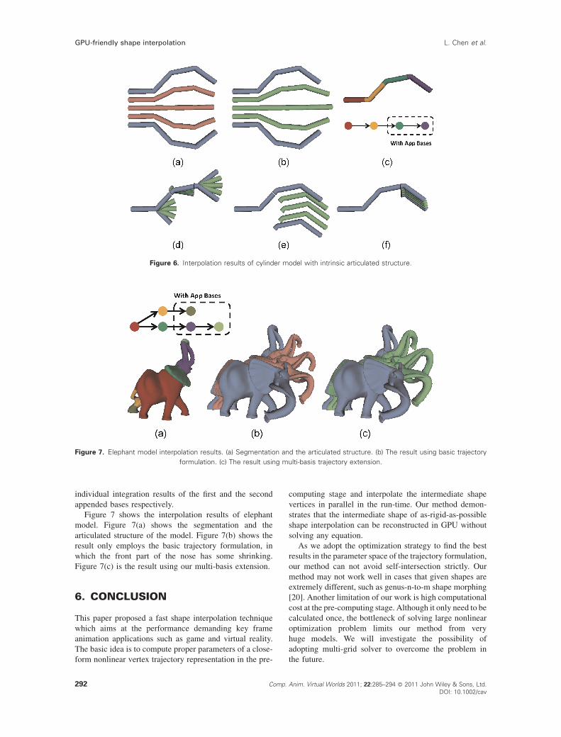
individual integration results of the first and the second

appended bases respectively.

Figure 7 shows the interpolation results of elephant

model. Figure 7(a) shows the segmentation and the

articulated structure of the model. Figure 7(b) shows the

result only employs the basic trajectory formulation, in

which the front part of the nose has some shrinking.

Figure 7(c) is the result using our multi-basis extension.

6. CONCLUSION

This paper proposed a fast shape interpolation technique

which aims at the performance demanding key frame

animation applications such as game and virtual reality.

The basic idea is to compute proper parameters of a close-

form nonlinear vertex trajectory representation in the pre-

computing stage and interpolate the intermediate shape

vertices in parallel in the run-time. Our method demon-

strates that the intermediate shape of as-rigid-as-possible

shape interpolation can be reconstructed in GPU without

solving any equation.

As we adopt the optimization strategy to find the best

results in the parameter space of the trajectory formulation,

our method can not avoid self-intersection strictly. Our

method may not work well in cases that given shapes are

extremely different, such as genus-n-to-m shape morphing

[20]. Another limitation of our work is high computational

cost at the pre-computing stage. Although it only need to be

calculated once, the bottleneck of solving large nonlinear

optimization problem limits our method from very

huge models. We will investigate the possibility of

adopting multi-grid solver to overcome the problem in

the future.

Figure 6. Interpolation results of cylinder model with intrinsic articulated structure.

Figure 7. Elephant model interpolation results. (a) Segmentation and the articulated structure. (b) The result using basic trajectory

formulation. (c) The result using multi-basis trajectory extension.



ACKNOWLEDGEMENTS

This work is supported by the China 863 project (No.

2009AA12Z229), China 973 Program (No.

2009CB320801), National Natural Science Foundation

of China (No. 61070073) and the Fundamental Research

Funds for the Central Universities (No. 2009QNA5023).

We also thank the anonymous reviewers for their helpful

comments and suggestions.

REFERENCES

1. Kraevoy V, Sheffer A. Cross-parameterization and

compatible remeshing of 3d models. Transactionson Graphics 23(3): 861–869. 2004.

2. Schreiner J, Asirvatham A, Praun E, Hoppe H. Inter-

surface mapping. ACM Transactions on Graphics2004; 23(3): 870–877.

3. Sumner RW., Popovic J 2004. Deformation

transfer for triangle meshes. In ACM SIGGRAPH2004 Papers (SIGGRAPH ’04), J Marks, (Ed.).

ACM, New York, NY, USA, 399–405.

DOI¼10.1145/1186562.1015736 http://doi.acm.

org/10.1145/1186562.1015736.

4. Alexa M, Cohen-Or D, Levin D. 2000. As-rigid-as-

possible shape interpolation. In Proceedings of the

27th annual conference on Computer graphics and

interactive techniques (SIGGRAPH ’00). ACM

Press/Addison-Wesley Publishing Co., New York,

NY, USA, 157-164. DOI¼10.1145/344779.344859

http://dx.doi.org/10.1145/344779.344859

5. Xu D, Zhang H,Wang Q, Bao H. 2005. Poisson shape

interpolation. In Proceedings of the 2005 ACM

symposium on Solid and physical modeling

(SPM ’05). ACM, New York, NY, USA, 267-

274. DOI¼10.1145/1060244.1060274 http://doi.

acm.org/10.1145/1060244.1060274

6. Choi MG, Ko H-S. Modal warping: Real-time simu-

lation of large rotational deformation and manipula-

tion. IEEE Transactions on Visualization andComputer Graphics 2005; 11(1): 91–101.

7. Alexa M. Recent advances in mesh morphing. Com-puter Graphics Forum 2002; 21(2): 173–196.

8. Alexa M. Differential coordinates for local mesh

morphing and deformation. The Visual Computer2003; 19(2): 105–114.

9. Sheffer A, Kraevoy V. 2004. Pyramid Coordinates

for Morphing and Deformation. In Proceedings of

the 3D Data Processing, Visualization, and Trans-

mission, 2nd International Symposium (3DPVT

’04). IEEE Computer Society, Washington, DC,

USA, 68-75. DOI¼10.1109/3DPVT.2004.99 http://

dx.doi.org/10.1109/3DPVT.2004.99.

10. Yu Y, Zhou K, Xu D, Shi X, Bao H, Guo B, et al.

Mesh editing with Poisson-based gradient field

manipulation. Transactions on Graphics 2004;

23(3): 644–651.11. Lipman Y, Sorkine O, Levin D, Cohen-Or. D. Linear

rotation-invariant coordinates for meshes. Trans-actions on Graphics 2005; 24(3): 479–487.

12. Kilian M, Mitra NJ, Pottmann H. 2007. Geometric

modeling in shape space. ACM Trans. Graph. 26 3.

Article 64 (July 2007). DOI¼10.1145/1276377.

1276457 http://doi.acm.org/10.1145/1276377.

1276457.

13. Der KG, Sumner RW, Popovic J. Inverse kinematics

for reduced deformable models. Transactions onGraphics 2006; 25(3): 1174–1179.

14. James DL, Twigg CD. Skinning mesh animations.

SIGGRAPH 2005; 399–407.

15. Feng W-W, Kim B-U, Yu. Y. Real-time data driven

deformation using kernel canonical correlation

analysis. SIGGRAPH 2008; 1–9.

16. Chu H-K, Lee. T-Y. Multiresolution mean shift clus-

tering algorithm for shape interpolation. IEEE Trans-actions on Visualization and Computer Graphics2009; 15(5): 853–866.

17. Choi MG, Woo SY, Ko. H-S. Real-time simulation of

thin shells. Computer Graphics Forum 2007; 26(3):349–354.

18. Sumner RW, Zwicker M, Gotsman C, Popovic J.

Mesh-based inverse kinematics. Transactions onGraphics 2005; 24(3): 488–495.

19. Botsch M, Sumner R, Pauly M, Gross M. Deformation

transfer for detail-preserving surface editing. In

Vision, Modeling & Visualization 2006; pp. 357–364.

20. Lee T-Y, Yao C-Y, Chu H-K, Tai M-J, Chen. C-C.

2006. Generating genus-n-to-m mesh morphing

using spherical parameterization: Research

Articles. Comput. Animat. Virtual Worlds 17,

3-4 (July 2006), 433-443. DOI¼10.1002/cav.v17:3/

4 http://dx.doi.org/10.1002/cav.v17:3/4.


293


AUTHORS’ BIOGRAPHIES

Lu Chen is a PhD student in theState Key Laboratory of CAD &CG at Zhejiang University. Hereceived his BS degree from theDepartment of Computer Science,Chu Kochen Honors Collegein 2005. His research interestsinclude geometric modeling andvirtual reality.

Jin Huang is an associate profes-sor in the State Key Laboratory ofCAD&CG at Zhejiang University,PR China. He received his PhDdegree in Computer Science fromZhejiang University in 2007 withExcellent Doctoral DissertationAward of China ComputerFederation (CCF). His research

interests include geometric processing and physical-based simulation. He has served as reviewer forACM SIGGRAPH, IEEE TVCG, Eurographics andCommittee Member of Pacific Graphics 2010.

Hongxin Zhang is an associate pro-fessor of the State Key Laboratoryof CAD & CG at Zhejiang Univer-sity, PR China. He received BS andPhD degrees in applied mathe-matics from Zhejiang University.His research interests include geo-metric modeling, texture synthesis,and machine learning.

Wei Hua is an Associate Professorin the State Key Lab ofCAD\&CG, College of ComputerScience at Zhejiang University,China. He received the Ph.D.degree in applied mathematicsfrom Zhejiang University in2002. Before that, he received hisBachelor’s degree from ZhejiangUniversity in 1996 in biomedical

engineering. His research interests include machinelearning, virtual reality and information retrieval.



Documents

GPU-friendly shape interpolation based on trajectory warping