Embed Size (px)
Citation preview
Graceful Labelings
By
Charles Michael Cavalier
Bachelor of ScienceLouisiana State University 2006
Submitted in Partial Fulfillment of the Requirements
for the Degree of Master of Science in
Mathematics
College of Arts and Sciences
University of South Carolina
2009
Accepted by:
Eva Czabarka, Major Professor
Joshua Cooper, Second Reader
James Buggy, Interim Dean of the Graduate School

Dedication
To my parents, Rickey and Susan.
ii

Acknowledgments
I would first and foremost like to thank Professor Eva Czabarka, my advisor, for
her steady support, guidance, and immense help in organizing and keeping me honest.
I would also like to thank my second reader, Professor Josh Cooper.
Additionally, I would like to thank my fellow graduate students and the other
people I’ve met through them. I could always count on Luke and Kate as well as
Mark, Ashley, and Matt for a good game of poker or pool. I would also like to thank
Aaron and Caroline for the great food they always donated to the office. Finally, I’d
like to thank Sam, Sarah, Rob, and Andrew. Without them, my graduate experience
would have been much less memorable.
iii
Abstract
Let T be a tree on n vertices and let f : V → {1, 2, . . . , n} be a valuation on
V (T ). Then f is called a graceful labeling of T if |f(v) − f(u)| is unique for each
edge vu ∈ E(T ). We will establish the connection between gracefully labeled trees
and the Ringel-Kotzig Conjecture, as well as survey several classes of trees that have
been proven graceful as a result of efforts to show that all trees are graceful.
iv

Contents
Dedication . . . . . . . . . . . . . . . . . . . . . . . . . . . . . . . . . . . . ii
Acknowledgments . . . . . . . . . . . . . . . . . . . . . . . . . . . . . . . iii
Abstract . . . . . . . . . . . . . . . . . . . . . . . . . . . . . . . . . . . . . iv
List of Figures . . . . . . . . . . . . . . . . . . . . . . . . . . . . . . . . . vi
Chapter 1. Introduction . . . . . . . . . . . . . . . . . . . . . . . . . . 1
Chapter 2. The Graph Labelings of Alexander Rosa . . . . . . . . 4
Chapter 3. Graceful Graphs . . . . . . . . . . . . . . . . . . . . . . . . 14
3.1. Graceful Graphs and a Classic Problem . . . . . . . . . . . . . . . . 14
3.2. The Graceful Tree Conjecture . . . . . . . . . . . . . . . . . . . . . . 18
Chapter 4. Adjacency Matrices of Graceful Graphs . . . . . . . . 43
Bibliography . . . . . . . . . . . . . . . . . . . . . . . . . . . . . . . . . . . 54
v

List of Figures
2.1 Cyclic Decomposition of K5 . . . . . . . . . . . . . . . . . . . . 10
2.2 Edges of K5 . . . . . . . . . . . . . . . . . . . . . . . . . . . . 10
3.1 Gracefully Labeled Kn for n = 2, 3, 4 . . . . . . . . . . . . . . . 15
3.2 K5 with Repeated Edge Labels . . . . . . . . . . . . . . . . . . 16
3.3 Gracefully Labeling a Caterpillar . . . . . . . . . . . . . . . . . 20
3.4 The Smallest Non-Caterpillar Tree . . . . . . . . . . . . . . . . 21
3.5 A Graceful Labeling of S(2, 2, 2, 2). . . . . . . . . . . . . . . . . 25
3.6 Graceful Tree T . . . . . . . . . . . . . . . . . . . . . . . . . . 31
3.7 The Graceful Tree T 3v . . . . . . . . . . . . . . . . . . . . . . . 32
3.8 Graceful trees T and S. . . . . . . . . . . . . . . . . . . . . . . 36
3.9 T∆S Labeled Gracefully. . . . . . . . . . . . . . . . . . . . . . 37
4.1 A Graceful Caterpillar . . . . . . . . . . . . . . . . . . . . . . . 45
4.2 Bipartite Graphs G1 and G2 with Compatible Labelings. . . . . 48
4.3 The Graceful Tree T = P4. . . . . . . . . . . . . . . . . . . . . 51
4.4 The Induced Graph T ◦K1,3. . . . . . . . . . . . . . . . . . . . 52
vi
Chapter 1
Introduction
The study of graph labelings has become a major subfield of graph theory. Very
often, the problems from this area draw attention due to their application to real
life situations or, in some cases, their history. Many of the most arduous problems
of graph theory are the easiest to state. The four-color theorem, for example, states
that a planar map can be colored using at most four colors in such a way that no
two bordering regions have the same color. This problem, originally hypothesized in
the early 1850’s, remained unsolved until the 1980’s, and its proof relies on the use of
computer software to check a large number of cases. Subsequent, more elegant proofs
have arisen, but the problem was unsolved for some one hundred eighty years.
Here, we investigate another somewhat longstanding problem in graph labelings.
The Graceful Tree Conjecture, which states that every tree graph on n vertices has
some vertex labeling using the numbers 1, 2, . . . , n such that the edge labeling obtained
from the vertex labeling by taking the absolute value of the difference of two adjacent
vertex labels assigns distinct edge labels. Alexander Rosa was the first to consider
such a labeling scheme as a method to prove the conjectures of Ringel and Kotzig
[15]. Ringel’s conjecture states that the complete graph K2m+1 can be decomposed
into 2m+1 subgraphs that are all isomorphic to a given tree on m edges. Kotzig later
conjectured that such a decomposition could be achieved cyclically. Rosa established
that these conjectures could be solved by showing that every tree can be labeled as
described above, which was ultimately termed graceful labeling.
1
In this monograph, we begin by introducing the definitions needed to state the
various conjectures and establish the early results of Rosa that facilitated an accessi-
bility to this problem leading to the publication of hundreds of papers on the subject.
While our main interest lies in the exposition of graceful labelings, we will see that
Rosa defines four labeling in [15] that are intimately related to each other. At times
we will give some of the results related to the other labelings. Chapter 2 contains
Rosa’s equivalence to the Ringel-Kotzig conjecture as well as other results pertaining
to the labelings.
In Chapter 3, we first focus on graceful graphs in general and a problem posed by
Golomb that utilizes graceful labelings in its solution. We then restrict to trees and
present several of the results toward the verification of the graceful tree conjecture.
Most of the results pertaining to this problem have come in the form of establishing
the gracefulness of relatively small classes of trees. Our discussion is broken into two
parts. First, we consider several families of trees shown to be graceful by more or less
standard techniques such as counting arguments, exhaustive techniques, and label
searches. The second phase of the discussion investigates the constructive methods
developed to build larger and larger graceful trees. Throughout this chapter, we offer
several examples of the constructions as it is often easier to understand them when
they are presented visually.
Finally, we consider adjacency matrices and their properties with respect to grace-
fully labeled graphs. We establish several conditions that give us an easy way to check
the gracefulness of a labeling given the graph’s adjacency matrix. We also provide
alternative ways to construct classes of graceful graphs by creating matrices from the
adjacency matrices of smaller graphs that induce larger graceful graphs.
These conjectures, which were made in the mid 1960’s, remain open to this day.
Kotzig and Rosa have referred to the graceful tree conjecture as a “graphical disease”
due to the inability to establish results reaching further than showing small classes of
trees are graceful. In fact, Frank Harary was the first to label problems as diseases, and
2
one of his originally diagnosed diseases was the aforementioned four-color theorem [7].
Nevertheless, work continues on the conjecture, more or less in the same direction.
Our goal here is to give a brief overview of the problem, as well as a flavor for
the techniques developed over the previous 4 decades. For a more comprehensive
treatment on graceful labelings, the reader is encouraged to reference A Dynamic
Survey of Graph Labeling maintained by Joseph A. Gallian [5].
3
Chapter 2
The Graph Labelings of Alexander Rosa
Here, we wish to survey the early types of graph labelings that were developed to
be used in investigating the Ringel-Kotzig Conjecture. We begin with a few central
definitions.
Definition 2.1. A graph G = (V,E) consists of a set V of vertices and a set E
of edges where each edge is of the form e = vi, vj for some vi, vj ∈ V , vi 6= vj. The
order of G is the number of vertices of G and is denoted by |G|. The size of G is the
number of edges of G and is denoted by ||G||.
In this thesis, a graph is a simple graph in that it has at most one edge between
any two vertices in V , and no edge has the same vertex as its endpoints. When more
than one graph is in question, we will sometimes denote the vertex and edge sets of
a graph G by V (G) = VG and E(G) = EG, respectively.
Definition 2.2. The degree of a vertex v in a graph G, denoted deg(v), is the
number of edges incident with v.
Definition 2.3. For a vertex v in a graph G, the neighborhood of v is the set
N(v) = {w ∈ V (G)|wv ∈ E(G)}.
Definition 2.4. A labeling (or vertex labeling) of a graph G, sometimes called a
valuation, is an injective map f : V → N that assigns to each vertex v ∈ V a unique
natural number.
4
Definition 2.5. A graph G is said to be bipartite if V (G) can be partitioned into
classes X = {x1, x2, . . . , xp} and Y = {y1, y2, . . . , yq} such that the edge xixj /∈ E(G)
for any i, j and the edge yky` /∈ E(G) for any k, `.
Definition 2.6. A graph G on n vertices is called the complete graph on n vertices
if the edge vivj ∈ E(G) for all 1 ≤ i, j ≤ n, i 6= j. We denote the complete graph of
order n by Kn.
Definition 2.7. A graph G is said to be the complete bipartite graph Kp,q if
V (G) can be partitioned into classes X = {x1, x2, . . . , xp} and Y = {y1, y2, . . . , yq}
such that the edge xixj /∈ E(G) for any i, j, the edge ypyq /∈ E(G) for any p, q, and
x`ym ∈ E(G) for all 1 ≤ ` ≤ p and 1 ≤ m ≤ q.
Definition 2.8. A walk between two vertices x and y in a graph G is a sequence
of vertices w1w2 . . . wk, where x = w1, y = wk, and for each i ∈ {1, 2, . . . , k − 1} we
have wiwi+1 ∈ E(G). The length of a walk is defined to be k − 1.
Definition 2.9. A closed walk in a graph is a walk that begins and ends with
the same vertex.
Definition 2.10. A path between two vertices x and y in a graph G is a walk
between x and y such that no vertex is repeated in the walk.
Definition 2.11. For vertices x, y ∈ V (G), the distance, d(x, y) = d(y, x), is the
length of a shortest path between x and y.
Definition 2.12. The graph G is called connected if for any two vertices x and
y in G, there is a path between x and y.
Definition 2.13. A cycle in a graph G is a closed walk of the form w1w2 . . . wk,
where k ≥ 3, and if for some i 6= j we have wi = wj, then {i, j} = {1, 2}.
Definition 2.14. A graph G is called acyclic if it contains no cycles.
5
Definition 2.15. A forest is an acyclic graph.
Definition 2.16. A tree is a connected acyclic graph.
Definition 2.17. A leaf of a tree T is a vertex v ∈ V (T ) such that deg(v) = 1.
Definition 2.18. The path graph on n vertices, Pn, is the graph whose edges
form a path of length n− 1.
Definition 2.19. A circuit in a graph G is a closed walk that traverses an edge
at most once.
Definition 2.20. A graph G is said to be Eulerian if there exists a circuit C ⊆ G
such that E(C) ≡ E(G).
We now state several theorems noting that the proofs can be found in any intro-
ductory graph theory text.
Theorem 2.21. A connected graph G is Eulerian if and only if the degree of each
vertex in G is even.
Theorem 2.22. For any tree T , there is a unique path between any two vertices
x and y in V (T ).
Theorem 2.23. Every tree is a bipartite graph.
Theorem 2.24. Every tree on n ≥ 2 vertices has at least two leaves.
Theorem 2.25. A tree with n vertices has n− 1 edges.
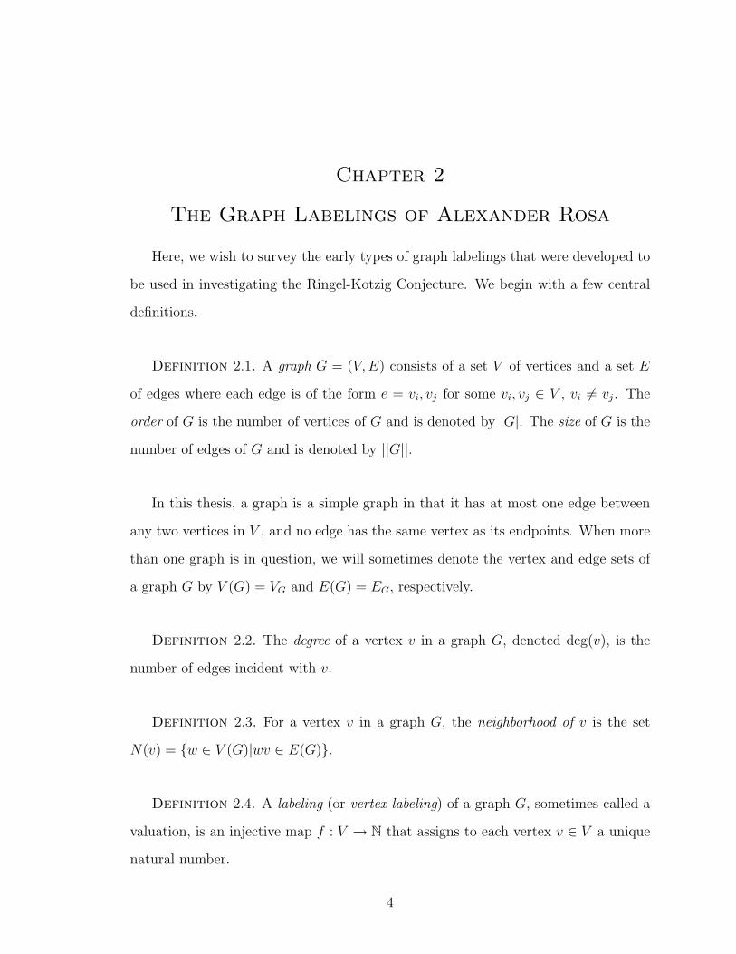
In 1966, Alexander Rosa published On Certain Valuations of the Vertices of a
Graph [15], which introduced several types of vertex labelings for simple graphs.
These constructions were the result of his work on a problem Ringel had presented
several years earlier in 1964, which was later strengthened by Kotzig. We now define
the labelings as introduced by Rosa.
6

Let G = (V,E) be a graph with n vertices and m edges, and let f : V → N
be a labeling of the vertices of V . Let ai = f(vi), for 1 ≤ i ≤ n. Define VΦG=
{a1, a2, . . . , an} to be the set of labels of the vertices of G given by f . For any edge
ek = vivj in E, let bk = |f(vi)−f(vj)| = |ai−aj|. We denote by EΦGthe set of values
bk of the edges of G induced by f .
Let f be a labeling of a graph G with m edges and consider the following condi-
tions:
(1) VΦG⊂ {0, 1, 2, . . . ,m}
(2) VΦG⊂ {0, 1, 2, . . . , 2m}
(3) EΦG= {1, 2, . . . ,m}
(4) EΦG= {x1, x2, . . . , xm} where xi = i or xi = 2m+ 1− i
(5) There exists x, with x ∈ {0, 1, 2, . . . ,m}, such that for any edge vivj of G,
either ai ≤ x and aj > x, or aj ≤ x and ai > x holds.
Then Rosa defines the following valuations:
• If f satisfies (1),(3), and (5), then f is called an α-valuation.
• If f satisfies (1) and (3), then f is called a β-valuation.
• If f satisfies (2) and (3), then f is called a σ-valuation.
• If f satisfies (2) and (4), then f is called a ρ-valuation.
From the definitions of these valuations, we see that there is a hierarchy structure
relating them. That is, an α-valuation is also a β, σ, and ρ-valuation. A β-valuation is
also a σ-valuation and a ρ-valuation. And finally, a σ-valuation is also a ρ-valuation.
Moreover, if there is an α-valuation of G, then G is a bipartite graph. While the
condition that G is bipartite is not sufficient for G to have an α-valuation, G being
complete bipartite is. For this reason, α-valuations are also referred to as bipartite
labelings.
Theorem 2.26. If a graph G has an α-valuation, then G is a bipartite graph.
7

Proof. Let G have an α-valuation and partition VΦG= {a0, a1, . . . , am} as fol-
lows. Define two sets by
A := {ai | ai > x}
B := {aj | aj ≤ x} .
Clearly, A ∩B = ∅. Also, for any edge e = a`am, the endvertices of e are in different
partitions. Thus G is a bipartite graph. �
Theorem 2.27. The graph Kp,q has an α-valuation.
Proof. [15] Let X and Y partition E and let V (X) = {x1, x2, . . . , xp} and
V (Y ) = {y1, y2, . . . , yq}. Then the valuation with f(xi) = i − 1 and f(yj) = jp is
an α-valuation. To see this, we note that Kp,q has m = pq edges. Without loss of
generality, we may assume that p ≤ q. Now, f maps V (Kp,q) into {0, 1, . . . , pq}, and
using x = p− 1 we have that for all edges xiyj, f(xi) ≤ x and f(yj) > x. Moreover,
|f(yj)− f(xi)| = f(yj)− f(xi) = jp− i+ 1. Since i ∈ {1, 2, . . . , p}, we have that for a
fixed j, {|f(yj)− f(xi)|∣∣i ∈ {1, 2, . . . , p}} = {(j− 1)p+ 1, (j− 1)p+ 2, . . . , jp}, which
gives that Ef(G) = {1, 2, . . . , pq}. Thus f is an α-valuation. �
These valuations provided the tools Rosa used to attack the conjectures of Ringel
and Kotzig. These conjectures, along with the necessary definitions follow.
Definition 2.28. Let G = (V,E) be a graph. Then the graph H = (V ′, E ′) is a
subgraph of G if V ′ ⊆ V and E ′ ⊆ E.
Definition 2.29. Let G1 = (V1, E1) and G2 = (V2, E2) be two graphs. Then the
union G1 ∪G2 = (V1 ∪ V2, E1 ∪ E2).
Definition 2.30. Let G be a graph. Then a decomposition, D, of G is a collection
of subgraphs Hi ⊆ G, i = 1, 2, . . . , k, such that E(Hi) ∩ E(Hj) = ∅ for all 1 ≤ i <
j ≤ k and G = ∪ki=1Hi.
8
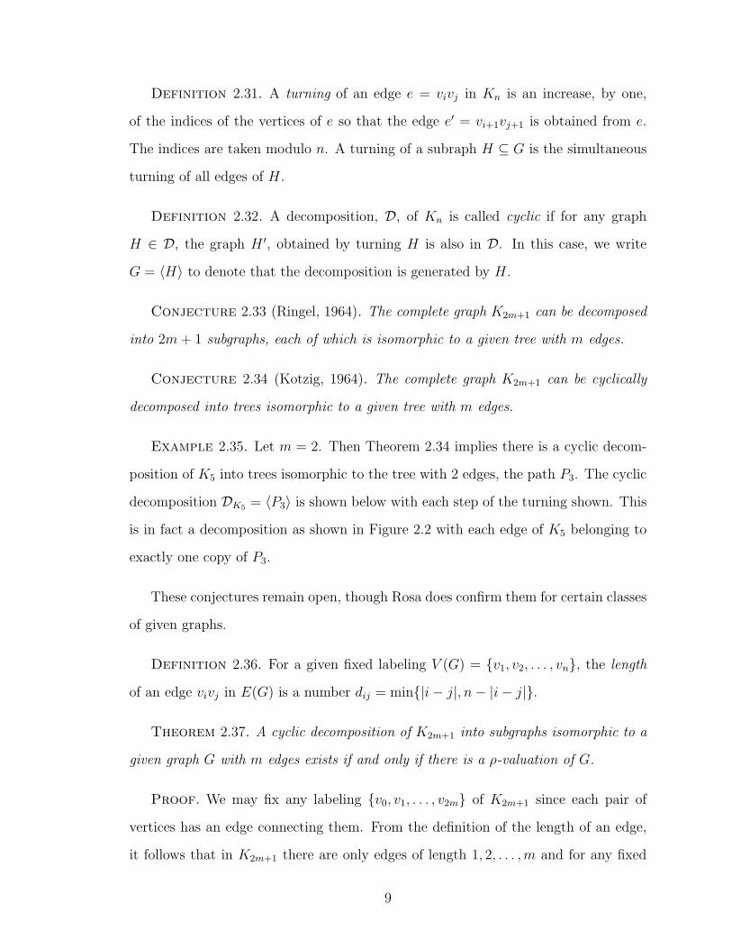
Definition 2.31. A turning of an edge e = vivj in Kn is an increase, by one,
of the indices of the vertices of e so that the edge e′ = vi+1vj+1 is obtained from e.
The indices are taken modulo n. A turning of a subraph H ⊆ G is the simultaneous
turning of all edges of H.
Definition 2.32. A decomposition, D, of Kn is called cyclic if for any graph
H ∈ D, the graph H ′, obtained by turning H is also in D. In this case, we write
G = 〈H〉 to denote that the decomposition is generated by H.
Conjecture 2.33 (Ringel, 1964). The complete graph K2m+1 can be decomposed
into 2m+ 1 subgraphs, each of which is isomorphic to a given tree with m edges.
Conjecture 2.34 (Kotzig, 1964). The complete graph K2m+1 can be cyclically
decomposed into trees isomorphic to a given tree with m edges.
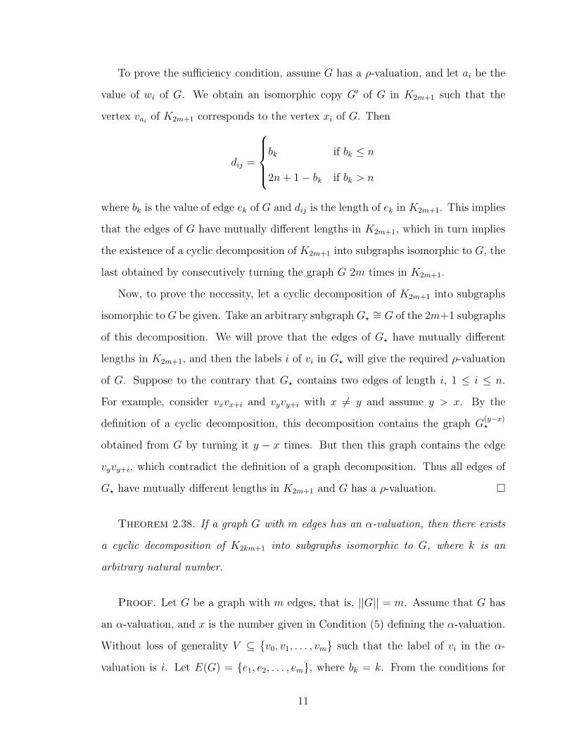
Example 2.35. Let m = 2. Then Theorem 2.34 implies there is a cyclic decom-
position of K5 into trees isomorphic to the tree with 2 edges, the path P3. The cyclic
decomposition DK5 = 〈P3〉 is shown below with each step of the turning shown. This
is in fact a decomposition as shown in Figure 2.2 with each edge of K5 belonging to
exactly one copy of P3.
These conjectures remain open, though Rosa does confirm them for certain classes
of given graphs.
Definition 2.36. For a given fixed labeling V (G) = {v1, v2, . . . , vn}, the length
of an edge vivj in E(G) is a number dij = min{|i− j|, n− |i− j|}.
Theorem 2.37. A cyclic decomposition of K2m+1 into subgraphs isomorphic to a
given graph G with m edges exists if and only if there is a ρ-valuation of G.
Proof. We may fix any labeling {v0, v1, . . . , v2m} of K2m+1 since each pair of
vertices has an edge connecting them. From the definition of the length of an edge,
it follows that in K2m+1 there are only edges of length 1, 2, . . . ,m and for any fixed
9
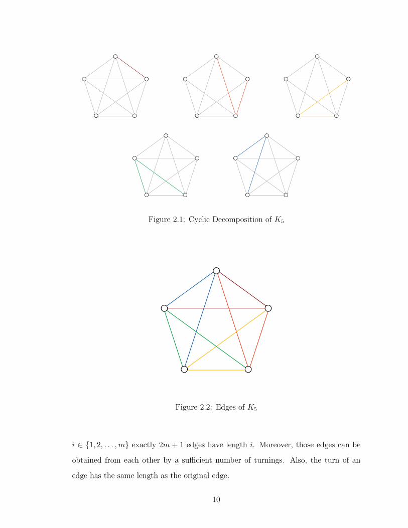
Figure 2.1: Cyclic Decomposition of K5
Figure 2.2: Edges of K5
i ∈ {1, 2, . . . ,m} exactly 2m + 1 edges have length i. Moreover, those edges can be
obtained from each other by a sufficient number of turnings. Also, the turn of an
edge has the same length as the original edge.
10
To prove the sufficiency condition, assume G has a ρ-valuation, and let ai be the
value of wi of G. We obtain an isomorphic copy G′ of G in K2m+1 such that the
vertex vaiof K2m+1 corresponds to the vertex xi of G. Then
dij =
bk if bk ≤ n
2n+ 1− bk if bk > n
where bk is the value of edge ek of G and dij is the length of ek in K2m+1. This implies
that the edges of G have mutually different lengths in K2m+1, which in turn implies
the existence of a cyclic decomposition of K2m+1 into subgraphs isomorphic to G, the
last obtained by consecutively turning the graph G 2m times in K2m+1.
Now, to prove the necessity, let a cyclic decomposition of K2m+1 into subgraphs
isomorphic to G be given. Take an arbitrary subgraph G?∼= G of the 2m+1 subgraphs
of this decomposition. We will prove that the edges of G? have mutually different
lengths in K2m+1, and then the labels i of vi in G? will give the required ρ-valuation
of G. Suppose to the contrary that G? contains two edges of length i, 1 ≤ i ≤ n.
For example, consider vxvx+i and vyvy+i with x 6= y and assume y > x. By the
definition of a cyclic decomposition, this decomposition contains the graph G(y−x)?
obtained from G by turning it y − x times. But then this graph contains the edge
vyvy+i, which contradict the definition of a graph decomposition. Thus all edges of
G? have mutually different lengths in K2m+1 and G has a ρ-valuation. �
Theorem 2.38. If a graph G with m edges has an α-valuation, then there exists
a cyclic decomposition of K2km+1 into subgraphs isomorphic to G, where k is an
arbitrary natural number.
Proof. Let G be a graph with m edges, that is, ||G|| = m. Assume that G has
an α-valuation, and x is the number given in Condition (5) defining the α-valuation.
Without loss of generality V ⊆ {v0, v1, . . . , vm} such that the label of vi in the α-
valuation is i. Let E(G) = {e1, e2, . . . , em}, where bk = k. From the conditions for
11
an α-valuation for each ` ∈ {1, 2, . . . ,m} we are given i`, j` such that e` = vi`vj`and
i` ≤ x and j` > x.
Let A = {vq ∈ V (G)|q ≤ x} and B = V (G) − A. For p ∈ {1, 2, . . . , k} we
will define the graph Gp = (V p, Ep) as follows: V p = A ∪ {vj+m(p−1) : vj ∈ B}
and Ep = {ep = vi`vj`+m(p−1)| ` ∈ {1, 2, . . . ,m}}. Note that by definition, Gp is
isomorphic to G, moreover, G1 = G. Also, any edge in Gp has an endpoint in A, and
another endpoint in the set {v(p−1)m, v(p−1)m+1, . . . , vpm}, so the Gp are edge-disjoint.
Moreover, for the edge ep we have that
|j` +m(p− 1)− i`| = (j` − i` +m(p− 1)) = `+m(p− 1) (1)
Let G′ =⋃k
p=1Gp. Since the Gp are edge disjoint, ||G′|| = k||G|| = km.
By our construction, V (G′) ⊆ {v0, . . . , vkm}. Define the valuation Φ : V (G′) →
{0, 1, . . . , km} by Φ(vq) = q. As for any edge of G′, there is a p ∈ {1, . . . , k} and
` ∈ {1, 2, . . . ,m} such that the edge is of the form vi` , v(p−1)m+j`, where i` ≤ x and
(p− 1)m + j` ≥ j` > x. Also, by equation (1) we have that EΦ(G′) = {1, 2, . . . , km}.
Thus, φ is an α- (and thus also a ρ-)valuation of G′, which, by Theorem 2.37 means
that there is a cyclic decomposition of K2km+1 into subgraphs isomorphic to G′. But
G′ is an edge-disjoint union of k copies of G, so this decomposition gives a cyclic
decomposition of K2km+1 into subgraphs isomorphic to G. �
If it were shown that every tree has an α-valuation, then both Ringel and Kotzig’s
conjectures would be confirmed. It has been proven, however, that not every tree
has an α-valuation. Since then, attention has been turned to investigating which
graphs have β-valuation. If it could be shown that every tree has a β-valuation,
then Kotzig’s Conjecture would be proven. This implies every tree has a ρ-valuation,
which would in turn prove Ringel’s Conjecture. In 1972, Solomon Golomb published
an article containing his results on graph labelings [6]. Among some of the labelings he
investigates were β-valuations, which he termed graceful labelings. It is now standard
to use the terms graceful labeling and graceful graph when referring to a graph that
12
admits a β-valuation. We follow suit and will use Golomb’s terminology from now
on. To repeat, therefore, the graceful labeling of a graph is defined as follows:
Definition 2.39. Let G be a graph on n vertices with m edges. G is said to
have a graceful labeling if there is a map f : V (G) → {0, 1, 2, . . . ,m} such that
|f(x) − f(y)| is unique for each edge xy ∈ E(G). We then necessarily have that
E(G) = {1, 2, . . . ,m}.
Finally, we wish to note that shifting the vertex labels by a positive integer k does
not affect whether or not the labeling is graceful. That is, if a graph is gracefully
labeled using labels from {0, 1, . . . ,m}, we get the same edge labels if we add k to
each vertex label, with each still being distinct. In general, we will be using labels
from {0, 1, . . . ,m}. In other cases, we will specify when we are using labels from
{k, 1 + k, . . . ,m+ k} by saying that we will be labeling beginning with k.
We now turn to the advancements in labeling graphs gracefully.
13

Chapter 3
Graceful Graphs
We now wish to restrict our discussion of graph labelings to one in particular —
graceful labelings. There have been many results in this direction. The majority of
the work done with this labeling applies to the class of trees, due obviously to its
connection with the decomposition theorems mentioned earlier. We will first look at
graceful graphs in general, then give results obtained for trees.
3.1. Graceful Graphs and a Classic Problem
Golomb [6] gives an application of a graph labeling, and gives a condition for the
labeling to be graceful. Suppose we are given solid bar of integer length `. We want
to carve n − 2 notches in it at integer distances from either end with the condition
that the distances between any two notches, as well as the distances from any notch
to either of the endpoints, are all distinct. This problem can be viewed as labeling
the vertices of the complete graph Kn with the elements of the set {0, 1, . . . , `} and
labeling each edge by taking the absolute value of the difference of its endvertices.
The problem is to find the smallest integer ` so that Kn can be labeled this way. In the
event that the vertices can be labeled using only numbers from N = {0, 1, 2, . . . ,(
n2
)},
with each edge label being distinct, then each number from N \{0} is used once. But
this simply implies that for this n, Kn has a graceful labeling.
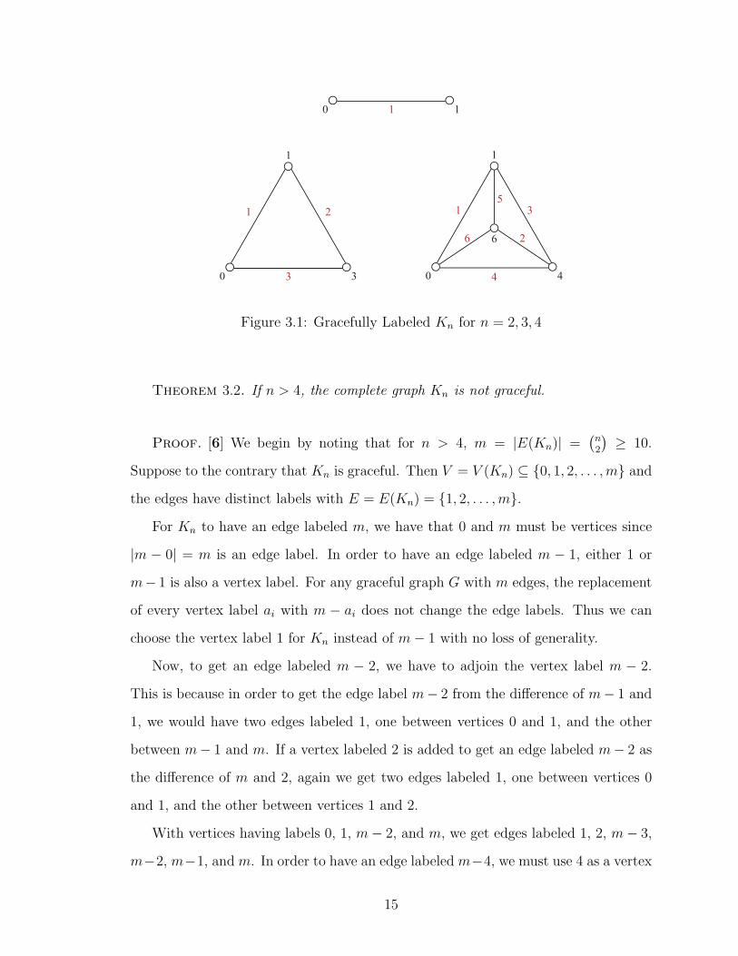
Example 3.1. Looking at the complete graphs on n vertices for n = 2, 3 and 4,
we have that the vertex labelings shown in Figure 3.1 are graceful.
It turns out that n = 4 is the largest n for which Kn can be labeled gracefully, as
proven by Golomb.
14
1
0 4
6
51
2
3
4
6
1
0 3
1 2
3
0 11
Figure 3.1: Gracefully Labeled Kn for n = 2, 3, 4
Theorem 3.2. If n > 4, the complete graph Kn is not graceful.
Proof. [6] We begin by noting that for n > 4, m = |E(Kn)| =(
n2
)≥ 10.
Suppose to the contrary that Kn is graceful. Then V = V (Kn) ⊆ {0, 1, 2, . . . ,m} and
the edges have distinct labels with E = E(Kn) = {1, 2, . . . ,m}.
For Kn to have an edge labeled m, we have that 0 and m must be vertices since
|m − 0| = m is an edge label. In order to have an edge labeled m − 1, either 1 or
m− 1 is also a vertex label. For any graceful graph G with m edges, the replacement
of every vertex label ai with m − ai does not change the edge labels. Thus we can
choose the vertex label 1 for Kn instead of m− 1 with no loss of generality.
Now, to get an edge labeled m − 2, we have to adjoin the vertex label m − 2.
This is because in order to get the edge label m− 2 from the difference of m− 1 and
1, we would have two edges labeled 1, one between vertices 0 and 1, and the other
between m− 1 and m. If a vertex labeled 2 is added to get an edge labeled m− 2 as
the difference of m and 2, again we get two edges labeled 1, one between vertices 0
and 1, and the other between vertices 1 and 2.
With vertices having labels 0, 1, m− 2, and m, we get edges labeled 1, 2, m− 3,
m−2, m−1, and m. In order to have an edge labeled m−4, we must use 4 as a vertex
15

label. This is because if we use 2, then we get two edges labeled 2 as a difference of
2 and 0 and as a difference of m− 2 and m.
If n = 5, then we should be done (we do have precisely 5 vertex labels). However,
in this case m = 10, and we have that m− 6 = 4, so there actually is a pair of edges
that have the same induced label, as shown in Figure 3.2. Thus, for n = 5 there
is no good labeling. We need to only consider the case when n > 5. In this case
m > 10 and so 4 < m − 6 and there clearly is no repetition of edge labels at this
point; moreover, we still need more labels. With vertices having labels 0, 1, 4, m− 2,
1
10
2 3
4
9
8
4
6 7
10
0
4
8
1
Figure 3.2: K5 with Repeated Edge Labels
and m, we have edge labels 1, 2, 3, 4, m − 6, m − 4, m − 3, m − 2, m − 1, and m.
Note that for K4, m = 6.
There is no way to obtain an edge labeled m − 5 because all choices for ways to
get such an edge label contains at least one vertex label that can’t be used. Adding
a vertex labeled m − 5 gives a second edge labeled m − 6 = (m − 5) − 1. Adding
a vertex labeled m − 4 gives two edges labeled 4 = m − (m − 4). Adding a vertex
16
labeled m − 1 gives duplicate edges labeled m − 2 = (m − 1) − 1. We cannot add a
vertex labeled 3 since we get two edges labeled 3− 1 = 2. Finally, our last choice is
adding a vertex labeled 5. This is not possible either since we get two edges labeled
5− 4 = 1. This is a contradiction to our assumption that Kn is graceful for all cases
when m− 5 > 4, which corresponds to n ≥ 5. �
Rosa also gives a necessary condition for a graph to be graceful.
Theorem 3.3. [15] If G is an Eulerian graph with m edges such that m ≡ 1 or
2 (mod 4), then G cannot be labeled gracefully.
Proof. Suppose to the contrary that G is graceful graph of size m ≡ 1 or
2 (mod 4) with an Eulerian circuit, and suppose G is graceful. Taking the sum
over all edge labels bi , we have
m∑i=1
bi =m∑
i=1
i =(m+ 1)m
2.
Now it is easy to see that if m ≡ 1 or 2 (mod 2), then
m∑i=1
bi ≡ 1 (mod 2)
However, for an arbitrary closed path C = a1, a2, . . . , am, a1, the edge labels are given
by
|a1 − a2|, |a2 − a3|, . . . , |am − a1|,
and, as |y| ≡ y (mod 2), the sum of the edge labels, with the indicies taken modulo
m+ 1, ism∑
i=1
|ai − ai+1| ≡m∑
i=1
(ai − ai+1) ≡ 0 (mod 2).
Thus, we have reached a contradiction and the claim is proven. �
17
3.2. The Graceful Tree Conjecture
The conjectures of Ringel and Kotzig have led to one of the most easily stated,
yet elusive conjectures in the realm of graph labelings.
Conjecture 3.4. All trees are graceful.
Many methods have been developed in hopes of resolving the nearly fifty year
old problem. Initially, Rosa established the gracefulness of several classes of trees in
[15]. Since then, other classes have been shown to admit graceful labelings. We will
investigate several of these classes, dividing the proof methods into constructive and
non-constructive classes.
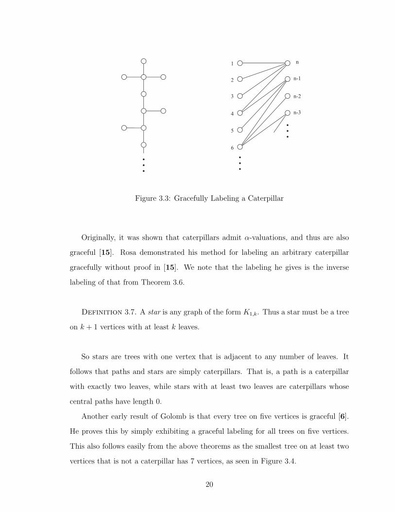
3.2.1. Several Classes of Graceful Trees. Here we consider several classes of
graceful trees. Unless otherwise stated, the graceful labelings given in this section are
starting from 1 in keeping with the convention used by the majority of publications
on graceful trees. The first class considered, caterpillars, was shown to be graceful by
Rosa in [15].
Definition 3.5. A caterpillar is a tree such that either every vertex is a leaf, or
by removing all leaves, we obtain a path. We call such a path a central path of the
caterpillar.
Now, it follows that a caterpillar has at least 2 vertices, and if it has at least 3
vertices, then the central path exists and is unique. The next theorem establishes the
gracefulness of caterpillars.
Theorem 3.6. All caterpillars are graceful.
Proof. [16] Let T be a caterpillar with n vertices. If n ≤ 2, then T is a path of
length one and we are done. So assume n ≥ 3, and let P = v0v1 . . . vk be the path
obtained from T by deleting the leaves of T . Since n ≥ 3, P has at least one vertex.
18

We now partition the vertex set of T as follows:
X = {x|x ∈ V (T ), d(v0, x) ≡ 0 (mod 2)}
Y = {y|y ∈ V (T ), d(v0, y) ≡ 1 (mod 2)} = V (T )−X.
We note that vi ∈ X if i is even and vi ∈ Y if i is odd. Label v0 with n. Label
the neighbors of v0 with 1, 2, 3, . . . where the neighbor getting the largest label is
v1. Assign labels n − 1, n − 2, n − 3, . . . to the neighbors of v1, other than v0, with
the largest label going to v2. Continue as follows. After v2i receives its label, assign
increasing integer labels to its neighbors other than v2i−1 starting with the smallest
unused label, assigning the largest label to v2i+1. Then, assign labels to the neighbors
of v2i+1, other than v2i, in decreasing order starting with the largest unused integer
smaller than n ending by labeling v2i+2.
The resulting labeling gives labels n, n− 1, . . . , n− |X|+ 1 to vertices in X while
vertices of Y are labeled 1, 2, . . . , |Y |. Moreover, since |X| + |Y | = n, the labels of
the vertices are all different.
Let `i be the label of the vertex vi. Clearly, `1 < `3 < . . . and `0 > `2 > . . ..
Now for an even i, if i /∈ {0, k}, the neighbors of vi have labels `i−1, `i−1 + 1, . . . , `i+1
and the induced edge labels are `i − `i+1, `i − `i+1 − 1, . . . , `i − `i−1. For an odd i,
if i 6= k, the neighbors of the vertex vi have labels `i−1, `i−1 + 1, . . . , `i+1, and the
induced edge labels are `i−1− `i, `i−1 + 1− `i, . . . , `i + 1− `i. The neighbors of v0 have
labels 1, 2 . . . , `1, the neighbors of vk have labels `k−1, `k−1 + 1, . . . , `k − 1 if k is even,
and `k + 1, `k + 2, . . . , `k+1 if k is odd. From all this it is easy to see that the n − 1
edge-labels are all different, the largest is n− 1 and the smallest is 1. Thus the given
labeling, as shown in Figure 3.3, is graceful. Note that the given labeling is also an
α-labeling, since conditions (1) and (3) are already checked, and condition (5) clearly
holds using x = |Y |. �
19
n
n-1
n-2
n-3
5
6
1
2
3
4
Figure 3.3: Gracefully Labeling a Caterpillar
Originally, it was shown that caterpillars admit α-valuations, and thus are also
graceful [15]. Rosa demonstrated his method for labeling an arbitrary caterpillar
gracefully without proof in [15]. We note that the labeling he gives is the inverse
labeling of that from Theorem 3.6.
Definition 3.7. A star is any graph of the form K1,k. Thus a star must be a tree
on k + 1 vertices with at least k leaves.
So stars are trees with one vertex that is adjacent to any number of leaves. It
follows that paths and stars are simply caterpillars. That is, a path is a caterpillar
with exactly two leaves, while stars with at least two leaves are caterpillars whose
central paths have length 0.
Another early result of Golomb is that every tree on five vertices is graceful [6].
He proves this by simply exhibiting a graceful labeling for all trees on five vertices.
This also follows easily from the above theorems as the smallest tree on at least two
vertices that is not a caterpillar has 7 vertices, as seen in Figure 3.4.
20
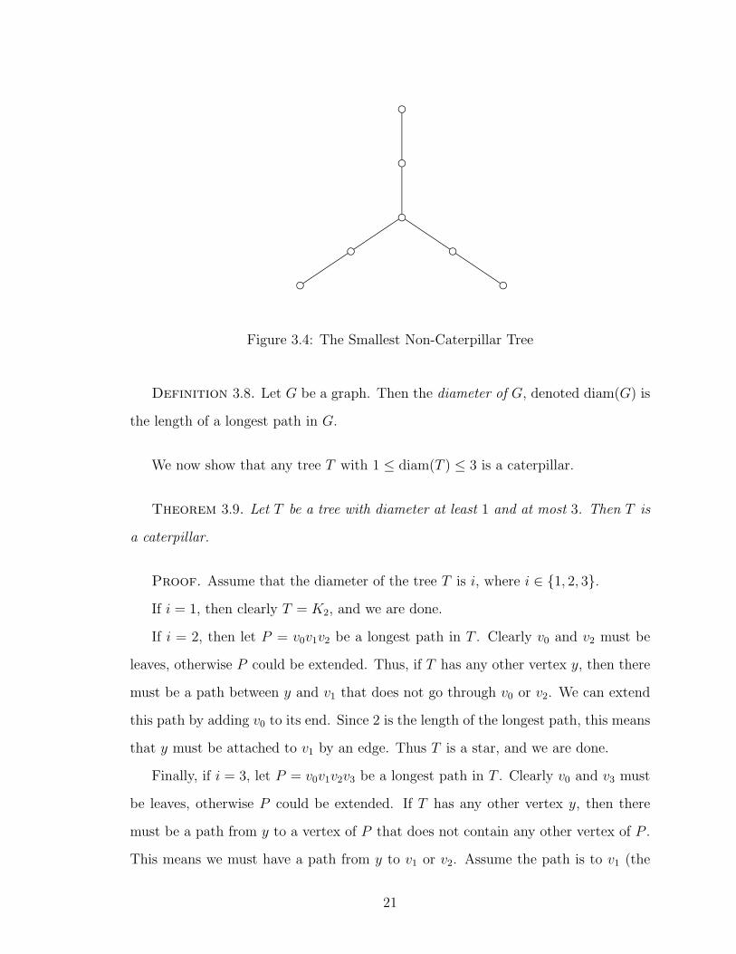
Figure 3.4: The Smallest Non-Caterpillar Tree
Definition 3.8. Let G be a graph. Then the diameter of G, denoted diam(G) is
the length of a longest path in G.
We now show that any tree T with 1 ≤ diam(T ) ≤ 3 is a caterpillar.
Theorem 3.9. Let T be a tree with diameter at least 1 and at most 3. Then T is
a caterpillar.
Proof. Assume that the diameter of the tree T is i, where i ∈ {1, 2, 3}.
If i = 1, then clearly T = K2, and we are done.
If i = 2, then let P = v0v1v2 be a longest path in T . Clearly v0 and v2 must be
leaves, otherwise P could be extended. Thus, if T has any other vertex y, then there
must be a path between y and v1 that does not go through v0 or v2. We can extend
this path by adding v0 to its end. Since 2 is the length of the longest path, this means
that y must be attached to v1 by an edge. Thus T is a star, and we are done.
Finally, if i = 3, let P = v0v1v2v3 be a longest path in T . Clearly v0 and v3 must
be leaves, otherwise P could be extended. If T has any other vertex y, then there
must be a path from y to a vertex of P that does not contain any other vertex of P .
This means we must have a path from y to v1 or v2. Assume the path is to v1 (the
21
other case can be handled similarly). If the path from y to v1 is not a single edge,
then we obtain a new path that is of length at least 4 by appending v2 and v3. Thus,
any vertex y of T not on P is attached by a single edge to either v1 or v2. Therefore,
T is a caterpillar. �
Huang, Kotzig, and Rosa [9] believed that showing all trees of diameter four were
graceful would be a major achievement in getting closer to proving the graceful tree
conjecture.
Let T (4) be the set of all trees of diameter 4. Let T (0, 4) be the singleton set
containing the path of length four. Now let T (1, 4) be the set of caterpillars of
diameter 4 excluding P5, and let T (2, 4) be the set of remaining trees of diameter
4. Then T (4) = T (0, 4) ∪ T (1, 4) ∪ T (2, 4), and these sets partition T (4). The
notation for these sets comes from T (i, n) containing the trees where there is a fixed
longest path of length n and a vertex x whose distance to the path is i, and all other
vertices have distance at most i from the path. Also, T (i, n) is non-empty provided
i ≤ bn2c, and these sets partition T (n), the set of trees on n vertices. Clearly any tree
from T (0, 4)∪ T (1, 4) is graceful. Showing the set T (2, 4) is graceful is slightly more
challenging. Huang et al. prove the following:
Theorem 3.10. If T ∈ T (2, 4), then T does not have an α-labeling.
The authors then proceed to show a special subclass of T (2, 4) is graceful. Shi-Lin
Zhao shows that the trees of T (2, 4) are graceful in [17].
Theorem 3.11. All trees of diameter 4 are graceful.
Zhao notes that although he was able to confirm that all trees of diameter four
are graceful, the result does not impact the general graceful tree conjecture as greatly
as hypothesized by Huang, Kotzig, and Rosa.
In 2001, the team of Hrnciar and Haviar established that trees of diameter 5 are
graceful in [8].
22
Theorem 3.12. All trees of diameter 5 are graceful.
Definition 3.13. LetG1 = (V1, E1) andG2 = (V2, E2) be graphs with no common
vertices, and let u ∈ V1 and v ∈ V2. By identifying the vertex u with the vertex v we
mean the procedure that results in the graph G = (V,E), where V = (V1 ∪ V2)−{v}
and
E = E1 ∪(E2 \ {vx|vx ∈ E2}
)∪ {ux|vx ∈ E2}
We will also call this the uv join of G1 and G2 and denote it by G1u ⊕G2
v.
Now, if G1 and G2 are trees, then clearly their uv-join is also a tree.
Definition 3.14. Let Gi = (Vi, Ei) be vertex-disjoint graphs with vi ∈ Vi. By
identifying the vertices v1, v2, . . . , vk we mean the result of the following recursive
procedure: For each j ∈ {2, 3, . . . , k} we define
G1v1⊕G2
v2⊕ . . .⊕Gj
vj=(G1
v1⊕G2
v2⊕ . . .⊕Gj−1
vj−1
)v1
⊕Gjvj
Definition 3.15. A spider is a tree consisting of m paths Px1 , Px2 , . . . , Pxm where
the vertices v1, v2, . . . , vm, with each vi a leaf of Pxi, are identified.
Huang et al. prove several results on spiders [9]. Recall that an α-valuation is
called a bipartite labeling.
Lemma 3.16. Let f1 be a bipartite labeling with labels starting at 0 of a tree S
with f1(u) = 0 for some u ∈ V (S). Let f2 be a graceful labeling (bipartite labeling,
resp.) with labels starting at 0 of a tree T with f2(v) = 0 for some v ∈ V (T ). Then
there is a graceful labeling (bipartite labeling, resp.) of Su ⊕ Tv.
23
Here we only sketch the proof. Define the labeling g of Su ⊕ Tv by
g(z) =
f ′1(z) if z ∈ V (T1) \ {u}, and f ′1(z) ≤ x
f ′1(z) +m if z ∈ V (T1) \ {u}, and f ′1(z) > x
f2(z) + x if z ∈ V (T2) \ {v}
x if z = u
where x is the value from condition (5) pertaining to a bipartite labeling, mi = ||Ti||,
and the valuation f ′1 is the inverse labeling of f1. That is, f ′1(z) = m1 − f1(z).
It is easy to see that an edge in T that has at least one endpoint on the vertices of T2
has the same value induced by g as the value induced by f2 on the corresponding edge
of T2. Thus, on these edges we have the induced edge-labels 1, 2, . . . ,m2. Therefore
we only need to show that the edge labels induced by g on the edges of T1 are m2 +
1, . . . ,m. That easily follows from the fact that f ′1 induces edge-labels {1, 2 . . . ,m1}
and all edges of T1 run between points z1z2 with f1(z1) ≤ x and f1(z2) > x.
We pause to note that it has been shown in [14] that for any path Pn and any
v ∈ V (Pn), there exists a graceful labeling f of Pn such that f(v) = 0. Also, there is
a bipartite labeling g of Pn such that g(v) = 0 for any v ∈ V (Pn) except when n = 5
and v is the middle vertex of P5.
Theorem 3.17. The spiders S(x1, x2, x3) with three legs are graceful.
Proof. This proof follows directly from the previous comment on labeling paths
and from Lemma 3.16. Identify a leaf from the path Px1 with a leaf of Px2 . The
resulting tree, T , is itself a path. Choose a graceful labeling of T such that the
identified vertex has label 0. Then, choose a bipartite labeling of Px3 such that one of
its leaves has label 0. Finally, joining T and Px3 and relabeling according to Lemma
3.16 results in the tree S(x1, x2, x3), which is labeled gracefully. �
24

It follows that every spider with three legs, except for S(2, 2, 2) has a bipartite
labeling. S(2, 2, 2) does not since there is no bipartite labeling of P5 with the central
vertex having label 0.
Theorem 3.18. The spiders S(x1, x2, x3, x4) with 4 legs are graceful.
Proof. [9] If at least one of x1, x2, x3, x4 is not 2, then without loss of generality
x1 + x2 6= 4. Let u be the central vertex of the spider S(x1, x2) = Px1+x2 and v be
the central vertex of the spider S(x3, x4) = Px3+x4 . We know that there is a bipartite
labeling of S(x1, x2) that labels u with 0 and a graceful labeling of S(x3, x4) that
labels v with 0. The result follows from Theorem 3.16. The only other possibility is
that x1 = x2 = x3 = x4 = 2. A graceful labeling of S(2, 2, 2, 2) is shown in Figure 3.5.
0
2 4 6 8
7 5 3 1
Figure 3.5: A Graceful Labeling of S(2, 2, 2, 2).
�
We will revisit spiders in Chapter 4 and show other subclasses that are graceful.
In 1998, Aldred and McKay published a paper outlining a computer based al-
gorithm they developed for testing trees for gracefulness [1]. Their result extended
Rosa’s result from [15] that all trees on at most 16 vertices are graceful.
Theorem 3.19. All trees on at most 27 vertices are graceful.
25
We now present the algorithm noting that they used two different search methods
in proving Theorem 3.19. For a tree T and an arbitrary labeling L of the vertices,
let z(T, L) denote the number of distinct edge labels induced by L. The goal of the
algorithm is to find a labeling L such that z(T, L) = |V (T )| − 1 as this would imply
the edge labels are distinct. For vertices v, w ∈ V (T ), define Sw(L; v, w) to be the
labeling achieved by swapping the labels on v and w given by L. Their first method,
whch relies on the parameter M , follows:
(1) Start with any arbitrary vertex labeling of T with labels {0, 1, . . . , n− 1}.
(2) If z(T, L) = n− 1, stop.
(3) For each pair of vertices {v, w}, replace L by L′ = Sw(L; v, w) if z(T, L′) >
z(T, L).
(4) If (3) finishes with L unchanged, replace L by Sw(L; v, w), where the vertices
{v, w} are chosen at random from the set of all {v, w} such that
(a) {v, w} has not been chosen during the most recent M times this step
has been executed.
(b) Sw(L; v, w) is maximal subject to (a).
(5) Repeat from step (2).
The authors note that this method sometimes gets stuck, but the problem is
resolved by restarting the algorithm using a different arbitrary initial labeling. The
parameter M prevents the algorithm from repeatedly cycling through a small number
of labelings. They add that M = 10 is usually suitable for smaller trees, but a useful
value for M increases as the size of the tree does. Their second method was an
exhaustive search over a restricted class of labelings. This second method was used
when the first search method did not succeed fast enough. They note that a graceful
labeling for a tree was typically used in determining the initial labeling for a larger
tree, and that the first method usually terminated quickly with a graceful labeling.
Their second method was invoked when this was not the case. Aldred and McKay also
26
illustrate the volume of their computations by informing us that there are 279,793,450
trees of order 26 and 751,065,460 trees of order 27.
3.2.2. Constructive Methods. Constructive methods for finding families of
graceful trees often originate with the goal of extending a known graceful tree or
collection of trees to a larger tree with a graceful labeling. In 1976, Cahit [3] posed
the question “Are all complete binary trees graceful?” This helped spark an interest
in graceful labelings and led to early research in constructive methods for finding
graceful trees. This section contains several constructions, each of which uses vertex
labelings starting with label 1.
Definition 3.20. An n-ary tree is a rooted tree in which the root has degree 0
or degree n, and every other non-leaf vertex has degree n+ 1.
Definition 3.21. The complete n-ary tree is an n-ary tree in which every root-
leaf path has length k. Denote by T (n, k) the complete n-ary tree with root-leaf path
length k.
It was Koh, Rogers, and Tan [11] who were able to verify an even stronger state-
ment. Let T be a graceful tree on n vertices where the vertex v has label n. Let
T p =
p·⋃i=1
Ti
for any p ∈ N and where each Ti is an isomorphic copy of T . That is, T p is the
disjoint union of p copies of T . Now, adjoin a new vertex v? to T p and the edge
{vi, v?} for all 1 ≤ i ≤ p, where vi is the isomorphic image of v in Ti. Let T p
v be the
graph constructed in this way. The claim, then, is that T pv is graceful.
Theorem 3.22. Let T be a gracefully labeled tree with n vertices, and let v ∈ V
be the vertex with label n. Then for any p ≥ 1, the graph T pv is graceful and v? has
the label np+ 1.
27

Proof. [11] For each vertex w in T , let d(w) (called the level of w) be the length
of the shortest path joining v and w in T . Given any integer p ≥ 1, we define a
valuation f ? from the vertex set of T pv onto the set {1, 2, . . . , np+ 1} in terms of the
valuation f and by the notion d(w) as follows:
(1) f ?(v?) = pn+ 1
(2) for each w in Ti∼= T , i = 1, 2, . . . , p,
f ?(w) =
i · n+ 1− f(w) if d(w) is even in T
(p+ 1− i)n+ 1− f(w) if d(w) is odd in T
Note that f ?(vi) = (i− 1)n+ 1 for each i = 1, 2, . . . , p, and f ?(v?) = pn+ 1 > f ?(w)
for each w in T pv − {v?}.
To show that f ? is a valuation, it suffices to show that f ? is one-to-one. Thus, let
u and w be two distinct vertices in ·∪Ti, i = 1, 2, . . . , p, and suppose to the contrary
that f ?(u) = f ?(w).
Case 1. Both u and w are in Ti for some i = 1, 2, . . . , p.
Clearly, u 6= w in T . Since f(u) 6= f(w), u and w can neither both lie on an
even level nor both on an odd level in T . Thus, by symmetry, we may suppose that
d(u) is even and d(w) is odd in T . By the definition of f ?, we get i · n + 1− f(u) =
(p + 1− i)n + 1− f(w), which implies n|p + 1− 2i| = |f(w)− f(u)| < n and forces
that p+ 1− 2i = 0. But then it follows that f(u) = f(w), which is not possible.
Case 2. u is in Ti and w is in Tj where i, j = 1, 2, . . . , p, and i 6= j.
Assume that d(u) is odd and d(w) is even in T . From the fact that f ?(u) = f ?(w),
it follows that (p+1−i)n+1−f(u) = jn+1−f(w). Thus we have n|j−(p+1−i)| =
|f(w) − f(u)| < n which implies that j − (p + 1 − i) = 0 and hence f(u) = f(w), a
contradiction.
28
Suppose either d(u) and d(w) are odd or d(u) and d(w) are even (say the latter).
Then i ·n+ 1− f(u) = jn+ 1− f(w), that is, n|j− 1| = |f(w)− f(u)|n, which again
implies that j = i, a contradiction.
Hence f ? is one-to-one and therefore is a valuation from the vertex set of T pv onto
the set {1, 2, . . . , pn+ 1}
To prove that f ? is a graceful valuation on T pv , it remains to be shown that the
edge labels of T pv induced by f ? are distinct. For each edge uw in T , let uiwi be the
corresponding copy of uw in Ti, and let f ?(uiwi) be the label induced by f ? on the
edge uiwi.
Now, since an edge in T must run between different a vertex of even and a vertex
of odd level, we may assume without loss of generality that u is at even level and w
is at odd level. Thus, we must have that
f ∗(uiwi) = |in+ 1− f(u)− (p+ 1− i)n− 1 + f(w)| = |(2i− p− 1)n+ f(w)− f(u)|.
This implies that
{f ∗(uiwi), f∗(up+1−iwp+1−i} = {|2i− p− 1|n+ f(uw), |2i− p− 1|n− f(u,w)}
For each integer i ∈ {1, 2 . . . , bp/2c} let
Si = {f ∗(uiwi), f∗(up+1−iwp+1−i)|uw ∈ E(T )}
= {(p+ 1− 2i)n+ f(uw), (p+ 1− 2i)n− f(u,w)|uv ∈ E(T )}.
Clearly, unless p is odd and i = p+12
, all integers in Si are pairwise distinct, and for
each x in Si, either (p− 2i)n < x < (p+ 1− 2i)n or (p+ 1− 2i)n < x < (p+ 2− 2i)n.
As T is graceful, the 2(n− 1) edges in Ti∪Tp+1−i are therefore assigned the following
29
2(n− 2) distinct integers:
(p− 2i)n+ 1,
(p− 2i)n+ 2,
...
(p− 2i)n+ (n− 1) and
(p+ 1− 2i)n+ 1,
...
(p+ 1− 2i)n+ (n− 1)
If p is odd and i = p+12
, then i = p+ 1− i, thus, by definition, S(p+1)/2 becomes
S(p+1)/2 = {f ∗(u(p+1)/2w(p+1)/2)|uw ∈ E(T )}
= {f(uw)|uw ∈ E(T )}
Note that if p is even, then the p isomorphic copies T1, . . . , Tp are grouped into p/2
pairs {T1, Tp}, {T2, Tp−1}, . . . , {Tp/2, Tp/2+1}. If p is odd, let
S(p+1)/2 = {f ?(u(p+1)/2w(p+1)/2)|uw is an edge in T}
By the definition of f ?, f ?(u(p+1)/2w(p+1)/2) = f(uw). Since f ?(v?v1) = p, . . . , f ?(v?vi) =
(p + 1 − i)n, . . . , f ?(v?vp) = n, it follows that each integer x = 1, 2, . . . , pn has been
assigned to an edge in T pv . Thus the proof is complete. �
The preceding proof allows us to take p copies of a graceful tree and identify the
largest labeled vertex in each copy with a leaf of the star K1,p. It follows immedi-
ately that every complete binary tree is graceful. Furthermore, all complete n-ary
trees are also graceful since they can be constructed inductively with the base case
corresponding to the star K1,n−1 on n vertices with central vertex labeled n and each
step of the induction producing a graceful tree using the labeling defined in Theorem
3.22.
30
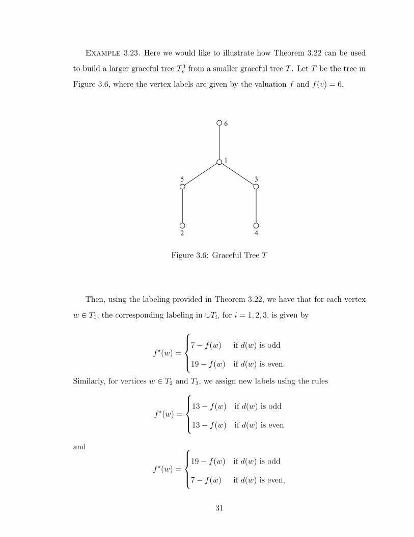
Example 3.23. Here we would like to illustrate how Theorem 3.22 can be used
to build a larger graceful tree T 3v from a smaller graceful tree T . Let T be the tree in
Figure 3.6, where the vertex labels are given by the valuation f and f(v) = 6.
5
1
2
3
4
6
Figure 3.6: Graceful Tree T
Then, using the labeling provided in Theorem 3.22, we have that for each vertex
w ∈ T1, the corresponding labeling in ·∪Ti, for i = 1, 2, 3, is given by
f ?(w) =
7− f(w) if d(w) is odd
19− f(w) if d(w) is even.
Similarly, for vertices w ∈ T2 and T3, we assign new labels using the rules
f ?(w) =
13− f(w) if d(w) is odd
13− f(w) if d(w) is even
and
f ?(w) =
19− f(w) if d(w) is odd
7− f(w) if d(w) is even,
31
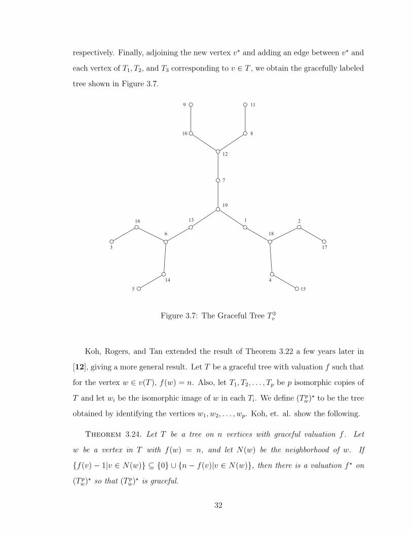
respectively. Finally, adjoining the new vertex v? and adding an edge between v? and
each vertex of T1, T2, and T3 corresponding to v ∈ T , we obtain the gracefully labeled
tree shown in Figure 3.7.
113
19
7
12
8
11
10
9
186
16 2
3 17
414
155
Figure 3.7: The Graceful Tree T 3v
Koh, Rogers, and Tan extended the result of Theorem 3.22 a few years later in
[12], giving a more general result. Let T be a graceful tree with valuation f such that
for the vertex w ∈ v(T ), f(w) = n. Also, let T1, T2, . . . , Tp be p isomorphic copies of
T and let wi be the isomorphic image of w in each Ti. We define (T pw)? to be the tree
obtained by identifying the vertices w1, w2, . . . , wp. Koh, et. al. show the following.
Theorem 3.24. Let T be a tree on n vertices with graceful valuation f . Let
w be a vertex in T with f(w) = n, and let N(w) be the neighborhood of w. If
{f(v) − 1|v ∈ N(w)} ⊆ {0} ∪ {n − f(v)|v ∈ N(w)}, then there is a valuation f ? on
(T pw)? so that (T p
w)? is graceful.
32
We omit the proof but note that it is similar to the proof of Theorem 3.22, and
note that the valuation f ? of (T pw)? given in the proof is as follows:
(1) f ?(w) = p(n− 1) + 1 and
(2) for every v ∈ Ti \ {w}, with i = 1, 2, . . . , p
f ?(v) =
(i− 1)(n− 1) + f(v) if d(w, v) is odd,
(p− i)(n− 1) + f(v) if d(w, v) is even.
Also appearing in [12] is a method for taking two arbitrary gracefully labeled trees
and combining them to obtain a larger graceful tree. Let T and S be graceful trees
under the valuations f1 and f2, respectively. Let V (T ) = {w1, w2, . . . , wm} and let v
be an arbitrary fixed vertex of S. Adjoin, to each wi, a copy Si of S by identifying
the isomorphic image of v in each Si, and wi. The tree obtained is denoted T∆S.
The m copies of S are pairwise disjoint and clearly, no new edges are added by this
operation.
Theorem 3.25. Let T and S be two graceful trees under the valuations f1 and f2,
respectively, and let |T | = m and |S| = n. Then there is a valuation f on T∆S such
that T∆S is graceful.
Proof. [12] Define a mapping f : T∆S → {1, 2, . . . ,mn} as follows:
We will denote the copy of a vertex z ∈ V (S) in the copy Si by zi. For each z in
V (S) and i ∈ {1, 2, . . . ,m}, we define
f(zi) =
(f1(wi)− 1)n+ f2(z) if d(v, z) is even,
(m− f1(wi))n+ f2(z) if d(v, z) is odd.
Since 1 ≤ f1(wi) ≤ m and 1 ≤ f2(z) ≤ n, it follows from the above definition that
f(zi) ∈ {1, 2, . . . ,mn}. We now show that f is one-to-one. Let ui ∈ Si and zj ∈ Sj
33
with ui 6= zj and f(zj) = f(ui). If d(v, u) is even and d(v, z) is odd, then
(f1(wi)− 1
)n+ f2(u) =
(m− f1(wj)
)n+ f2(z),
which gives that
n− 1 ≥ |f2(u)− f2(z)| = n|[m+ 1− (f1(wi) + f2(wj))]| ≥ 0.
Thus f2(u) = f2(z), which is a contradiction. If both d(v, u) and d(v, z) are either
even or odd, we again reach a contradiction by applying a similar argument, showing
that f is one-to-one. Thus f is a valuation.
We now show that the edge labels of T∆S are distinct. First, note that f(wiwj) =
nf1(wiwj) if wiwj is an edge in T . Indeed,
f(wiwj) = |f(wi)− f(wj)|
= |(f1(wi)− 1)n+ f2(v)− (f1(wj)− 1)n− f2(v)|
= n|f1(wi)− f1(wj)|
= nf1(wiwj).
Now consider an edge in T∆S other than the ones of the form wiwj. This edge then
must be an edge of Si for some i, i.e. it is of the form uizi for some uz ∈ E(S).
Assume without loss of generality that d(v, u) is even and d(v, z) is odd. Observe
that
f(uizi) = |(f1(wi)− 1)n+ f2(u)− (m− f1(wi))n− f2(z)|
= |(2f1(wi)−m− 1)n+ (f2(u)− f2(z))|,
which clearly is not a multiple of n. Thus it suffices to show that f(uizi) 6= f(u′jz′j)
for any pair of distinct edges uv and u′jz′j in T∆S where uz, u′z′ ∈ E(S), and i, j ∈
{1, 2, . . . ,m}. To this end, assume also without loss of generality that u′z′ is an edge
34
of S and say d(u′, v) is even and d(z′, v) is odd. Then we have
f(u′jz′j) = |(2f1(wj)−m− 1)n+ (f2(u)− f2(z))|.
Assume f(uizi) = f(u′jz′i), and for simplicity, let a = (2f1(wi)−m− 1)n, b = f2(u)−
f2(z), c = (2f1(wj)−m−1)n, and d = f2(u′)−f2(z′). We want to show that the edges
uizi and u′jz′j must be the same. Note that from the definition, |b| = f2(uz) ≤ n− 1
and |d| ≤ f2(u′z′) ≤ n − 1. We may also assume without loss of generality that
a+ b ≥ c+ d. We have the following cases:
Case 1. a+ b ≥ 0 and c+ d ≥ 0.
In this case we have a+ b = c+ d. Thus, a− c = d− b. In other words,
(2n)|f1(wi)− f1(wj)| = |d− b| ≤ 2(n− 1)
which forces that f1(wi) = f1(wj). That is, i = j. From i = j and d = b we get
f2(uz) = f2(u′z′), which means that u = u′ and z = z′. Thus u′jz′j = uizi, and the
two edges were not different to begin with.
Case 2. a + b ≥ 0, c + d ≥ 0. If this is the case we have that a + b = −c− d, which
means that if c ≥ 0 then
(2f1(wi)−m− 1)n+ b = (m+ 1− 2f1(wj))n− d
otherwise
(2f1(wi)−m− 1)n+ b = (2f1(wj)−m− 1))n− d.
Both of these lead to the conclusion that 2n divides b+d. But, since |b+d| ≤ |b|+|d| ≤
2(n − 1), this is only possible if b = −d, from which we get that f2(u) − f2(z) =
f2(z′) − f2(u′). But this means that the uv and u′v′ edges are the same in S, but
u = z′ and z = u′. This contradicts the assumption that d(u, v) is even but d(z′, v) is
odd. Thus, this case can not occur and the proof is complete. �
35
This ∆-construction essentially uses one graceful tree, say T , as a type of support,
and adjoins to each vertex in T a copy of another graceful tree S by identifying each
vertex of T with an arbitrary, but fixed vertex in each copy of S.
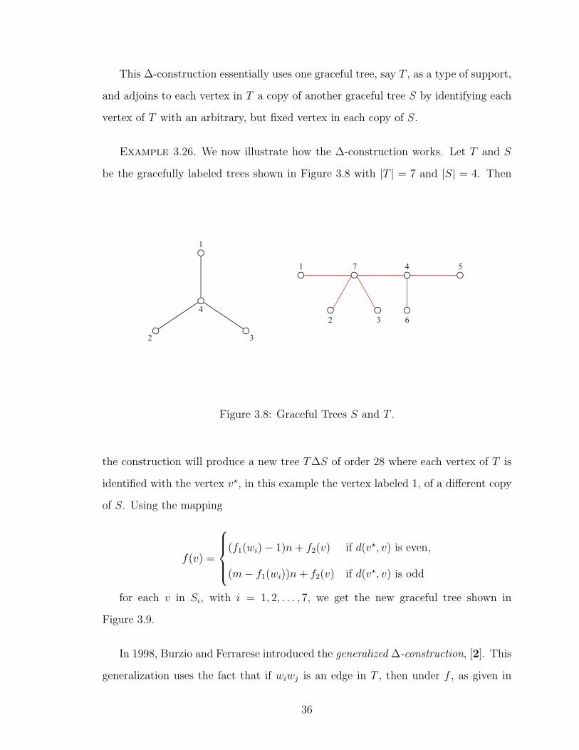
Example 3.26. We now illustrate how the ∆-construction works. Let T and S
be the gracefully labeled trees shown in Figure 3.8 with |T | = 7 and |S| = 4. Then
1
2 3
4
1 7 4 5
2 3 6
Figure 3.8: Graceful Trees S and T .
the construction will produce a new tree T∆S of order 28 where each vertex of T is
identified with the vertex v?, in this example the vertex labeled 1, of a different copy
of S. Using the mapping
f(v) =
(f1(wi)− 1)n+ f2(v) if d(v?, v) is even,
(m− f1(wi))n+ f2(v) if d(v?, v) is odd
for each v in Si, with i = 1, 2, . . . , 7, we get the new graceful tree shown in
Figure 3.9.
In 1998, Burzio and Ferrarese introduced the generalized ∆-construction, [2]. This
generalization uses the fact that if wiwj is an edge in T , then under f , as given in
36
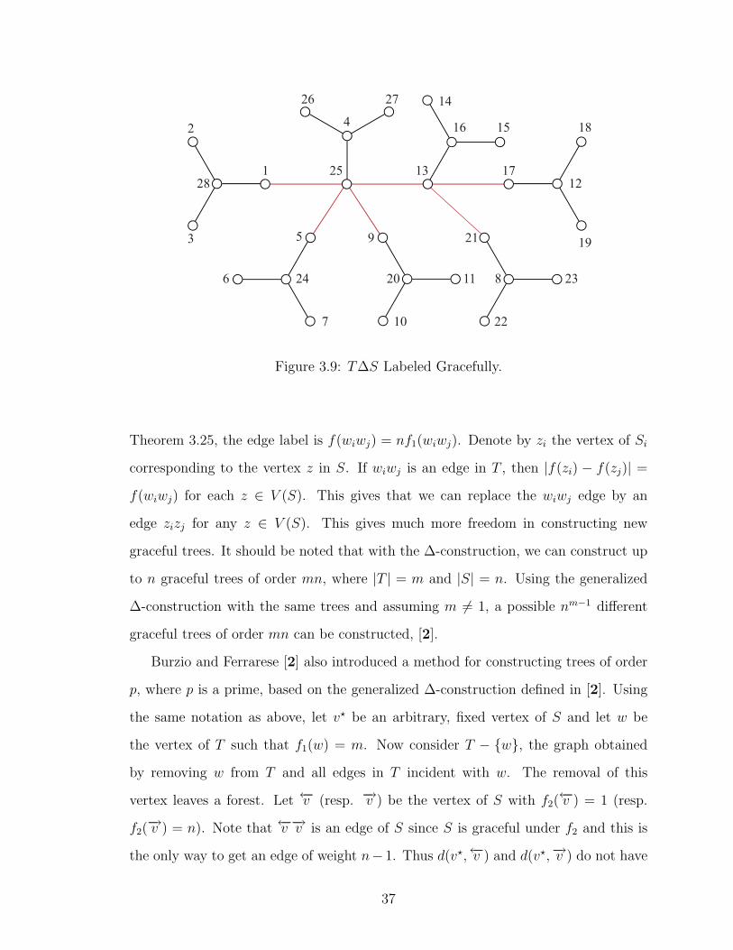
1 25 13 17
2
3
28
26
4
27 14
16 15
5
246
7 10 22
9 21
20 11 8 23
19
18
12
Figure 3.9: T∆S Labeled Gracefully.
Theorem 3.25, the edge label is f(wiwj) = nf1(wiwj). Denote by zi the vertex of Si
corresponding to the vertex z in S. If wiwj is an edge in T , then |f(zi) − f(zj)| =
f(wiwj) for each z ∈ V (S). This gives that we can replace the wiwj edge by an
edge zizj for any z ∈ V (S). This gives much more freedom in constructing new
graceful trees. It should be noted that with the ∆-construction, we can construct up
to n graceful trees of order mn, where |T | = m and |S| = n. Using the generalized
∆-construction with the same trees and assuming m 6= 1, a possible nm−1 different
graceful trees of order mn can be constructed, [2].
Burzio and Ferrarese [2] also introduced a method for constructing trees of order
p, where p is a prime, based on the generalized ∆-construction defined in [2]. Using
the same notation as above, let v? be an arbitrary, fixed vertex of S and let w be
the vertex of T such that f1(w) = m. Now consider T − {w}, the graph obtained
by removing w from T and all edges in T incident with w. The removal of this
vertex leaves a forest. Let ←−v (resp. −→v ) be the vertex of S with f2(←−v ) = 1 (resp.
f2(−→v ) = n). Note that ←−v −→v is an edge of S since S is graceful under f2 and this is
the only way to get an edge of weight n− 1. Thus d(v?,←−v ) and d(v?,−→v ) do not have
37
the same parity. Define a new valuation f = f2 if d(v?,←−v ) is even and f = n+ 1− f2
if d(v?,←−v ) is odd. Construct a new graph G = (T − {w})∆S, which has (m − 1)n
vertices and will generally be a proper forest. We define the valuation f on G as
follows:
f(vi) =
(f1(w)− 1)n+ f(v) if d(v?, v) is even,
(m− 1− f1(wi))n+ f(v) if d(v?, v) is odd.
for each vertex v ∈ V (Si), i = 1, 2, . . . ,m− 1.
The values for each edge vv′ of G, given by |f(v) − f(v′)|, are distinct. Since
f1(w) = n, it follows that the edge label values not appearing are the multiples npk,
where each pk is the weight of the edge wwk, the edge incident with w in T . To
recover the missing values, add to G a new vertex u and for each k such that wwk is
an edge in T , add the edges u←−v (k) to G if f = f2 (resp. u−→v if f = f ′2) where ←−v (k)
(resp. −→v (k)) is the corresponding vertex of←−v (resp. −→v ) in Sk. We denote this graph
by T∆+S.
Theorem 3.27. The mapping f+ : T∆+S → {1, 2, . . . , (m− 1)n+ 1} defined by
f+(v) = f(v) for each v ∈ V (G)
f+(u) = (m− 1)n+ 1
is a graceful valuation on T∆+S.
Proof. [2] If f = f2, we need only show that |f+(u)− f+(←−v (k))| = npk. But
|f+(u)− f+(←−v (k))| = |(m− 1)n+ 1− [(f1(wk)− 1)n+ 1]|
= |(m− 1)n+ 1− [(m− pk − 1)n+ 1]|
= |pkn| = pkn
The proof for when f = f ′2 is similar. �
38
Using these results, Burzio and Ferrarese were able to show that subdivision
graphs are graceful.
Definition 3.28. Let G be a graph. The graph obtained by replacing each edge
uv of G by a new vertex w and the edges uw and vw is called the subdivision graph
of G, denoted S(G).
Theorem 3.29. The subdivision graph of a graceful tree is a graceful tree.
Proof. [2] Let T be a graceful tree under valuation f1 and a let |T | = m. Let
w ∈ V (T ) be the vertex such that f1(w) = m. Let S = P2, the path on two vertices,
be graceful under f2 with vertices ←−v ,−→v such that f2(←−v ) = 1 and f2(−→v ) = 2. Fix
v? = ←−v in S and obtain T∆+S with the ∆+-construction. Using the generalized
∆-construction, connect the copies Si and Sj in T −{w} by the edge ←−v (i)←−v (j) (resp.
−→v (i)−→v (j)) if d(wj, w) = d(wi, w) + 1 is odd (resp. even). Then S(T ) = T∆+S is the
subdivision graph of T and S(T ) is graceful by Theorem 3.27. �
Koh et al., in [10], summarize their previous results from [11] and [12] as well as
define and explore a class of trees they call interlaced trees. Here, they add conditions
to those for graceful labelings and give methods for generating larger interlaced trees.
Definition 3.30. Let T be a tree on n vertices. The vertex b ∈ V (T ) for which
f(b) = 1 under the valuation f is the base of the valuation f .
For any vertex v ∈ T , let E(v) be the set of all vertices u in T for which d(v, u) is
even. Note that v ∈ E(v), and d(v, v) = 0. Let s(v) = |E(v)|.
Definition 3.31. If T is graceful under f with base b, then the size, s, of T
under f is s = s(b).
Definition 3.32. Let T be a tree, and let b be the base of the valuation f of T .
Then f is a parity valuation if it induces, by restriction, a bijection between E(b) and
the set {1, 2, . . . , s}.
39

Definition 3.33. An interlaced valuation f of T is a graceful valuation that is
also a parity valuation. Interlaced trees are trees admitting interlaced valuations.
In order to state and prove the following two results, let T1 and T2 be disjoint
trees on n1 and n2 vertices having graceful valuations f1 and f2 with bases b1 and
b2, respectively. Let s1 and s2 be the sizes of T1 and T2 when f1 or f2 is interlaced.
These constructions give a way to combine interlaced trees to obtain graceful trees
and give conditions for which the resulting tree is also interlaced.
Theorem 3.34. Let T1 be an interlaced tree under f1 and let x ∈ V (T1) be the
vertex for which f1(x) = s1. Let T be the tree obtained from T1 and T2 by identifying
x ∈ V (T1) with b2 ∈ V (T2). Then T is graceful. Furthermore, if f2 is also interlaced,
then T is an interlaced tree.
Proof. [10] We define the valuation f of T as follows:
f(v) =
f1(v) v ∈ ET1(b1)
f1(v) + n2 − 1 v /∈ ET1(b1) ∪ V (T2)
f2(v) + s1 − 1 v ∈ V (T2) \ {b2}
Now by definition, f(ET1) = f1(ET1) = {1, 2, . . . , s1}, f(V (T1) \ ET1) = {s1 + n2, s1 +
n2 + 1, . . . , n1 +n2− 1} and f(V (T2)−{b2}) = {s1 + 1, s1 + 2, . . . , s1 +n2− 1}. Thus,
f is a valuation assigning labels from {1, 2, . . . , n1 + n2 − 1}.
Since the edges of T1 are between vertices of ET1 and V (T1) \ ET1 , we get that
Ef(T1) = {n2, n2 + 1, . . . , n2 + n1 − 2}. On the other hand, Ef(T2) = {1, 2 . . . , n2 − 1}.
Thus, f is graceful. Also, when f2 is interlaced, f is an interlaced labeling of T with
base b1 and size s1 + s2− 1, since b1 and b2 = x are an even distance from each other.
Consequently, ET (b1) = ET1(b1)∪ET2(b2) and f(ET ) = {1, 2, . . . , s1, s1 + 1, . . . , s1 + s2−
1}. �
40
The next theorem gives a method for taking the disjoint union of two interlaced
trees and adding an edge between a vertex from each to obtain a new graceful tree.
Conditions are also given for when the resulting tree is interlaced.
Theorem 3.35. Suppose f1 and f2 are interlaced labelings of T1 and T2, respec-
tively. Also, suppose there are vertices u1 ∈ V (T1) and u2 ∈ V (T2) such that either:
(1) f1(u1)− f2(u2) = s1 < f1(u1), or
(2) n2 + f1(u1)− f2(u2) = s1 ≥ f1(u1)
Let T be the tree obtained by joining u1 and u2 by a new edge. Then T is graceful.
Furthermore, if in the two cases above we also have
(1) f2(u2) ≤ s2, or
(2) f2(u2) > s2,
then T is also an interlaced tree.
Proof. [10] Define f on V (T ) as follows:
f(v) =
f1(v) v ∈ ET1(b1)
f1(v) + n2 v /∈ ET1(b1) ∪ V (T2)
f2(v) + s1 v ∈ V (T2).
Then, f(ET1(b)) = {1, 2 . . . , s1}, f(V (T1) \ ET1(b1)) = {s1 + n2 + 1, s1 + n2 +
2, . . . , n1 + n2} and f(V (T2)) = {s1 + 1, s1 + 2, . . . , s1 + n2}, so f is a valuation that
assigns labels in {1, 2, . . . , n1 + n2}.
Now since edges of T1 run between a vertex of ET1(b1) and a vertex of V (T )\ET1(b1),
Ef(T1) = {n2 + 1, n2 + 1, . . . , n2 + n1}, and Ef(T2) = {1, 2, . . . , n2 − 1}. Moreover, in
case (1), since we have u1 /∈ ET1(b1),
|f(u1)− f(u2)| = f(u1)− f(u2) = f1(u1) + n2 − (f2(u2) + s1) = n2,
41
and in case (2), when u1 ∈ ET1 ,
|f(u1)− f(u2)| = f(u2)− f(u1) = (f2(u2) + s1)− f1(u1) = n2.
Thus, in either case we have that the new edge has weight n2. Hence the edges of T
carry all possible weights in {1, 2, . . . , n1 + n2 − 1} and f is a graceful labeling of T .
Additionally, if f2(u2) ≤ s2 when f1(u1) > s1 or f2(u2) > s2 when f1(u1) ≤ s1, then
it follows that the bases b1 and b2 are an even distance apart. So T is an interlaced
tree with size s = s1 + s2 and base b = b1. �
42
Chapter 4
Adjacency Matrices of Graceful Graphs
Definition 4.1. Let G be a graph with V (G) = {v1, v2, . . . , vn}. Then the matrix
AG = [aij] defined by
aij =
1 if vivj ∈ E(G)
0 otherwise
is called the adjacency matrix of G.
Definition 4.2. Let G be a graph with m = ||G|| and a valuation f : V (G) →
{1, 2, . . . ,m+ 1}. Then the (m+ 1)× (m+ 1) matrix AG = [aij] defined by
aij =
1 if xy ∈ E(G) for f(x) = i and f(y) = j
0 otherwise.
is called the generalized adjacency matrix of G induced by the valuation f . For
simplicity, we will assume in this chapter that V (G) ⊆ {v1, v2, . . . , vm+1} and f is
given by f(vi) = i.
Note that when G is a tree then the concepts in Definitions 4.1 and 4.2 agree.
Also, the generalized adjacency matrix allows (all zero) rows/columns corresponding
to missing labels; while in the adjacency matrix such rows correspond to vertices of
degree 0. If two graphs have the same (or similar) adjacency matrix, then they are
isomorphic, but if two graphs have the same generalized adjacency matrix, they may
not be isomorphic. However, we get isomorphic graphs if we leave out the vertices of
degree 0 from both.
43
Adjacency matrices are quite useful as they encode many of the corresponding
graphs’ characteristics. For example, vertex labeling, vertex adjacency, vertex degree,
and other graph features are quickly ascertained by looking at a graph’s adjacency
matrix. In fact, the field of spectral graph theory makes use of adjacency matrices
and their eigenvalues, eigenvectors, characteristic functions, etc., in investigating in-
variant graph properties. One particularly nice property of adjacency matrices is that
one can find the number of walks of varying lengths between vertices by looking at
multiplicative powers of the matrix. As stated earlier, we are only considering simple
undirected graphs. This means that the corresponding adjacency matrices will be
symmetric since there is no orientation on the edges and thus there is no distinction
drawn between edges vivj and vjvi. The property that all the graphs considered are
simple guarantees that the main diagonal entries of the adjacency matrices will be
zeros as a one on the main diagonal corresponds to a loop in the graph. Our interest
in adjacency matrices is motivated by their properties when the corresponding graph
is labeled gracefully.
Definition 4.3. Let A be an n × n matrix. Then the kth diagonal line of A is
the collection of entries Dk = {aij| j − i = k}, counting multiplicity.
So it is clear that 0 ≤ |k| ≤ n − 1. When A = AG is a (generalized) adjacency
matrix, A is symmetric and Dk = D−k. Thus we make the convention that the entry
1 corresponding to an edge between vertices vi and vj lies in the |j− i|th diagonal line
and the edge label for that edge is |j − i|, assuming f(vi) = i for each i = 1, 2, . . . , n
and f is a valuation on G. We now prove a theorem characterizing the adjacency
matrices of graceful graphs.
Theorem 4.4. Let G be a labeled graph and let AG be the generalized adjacency
matrix for G. Then AG has exactly one entry 1 in each diagonal line, except the main
diagonal of zeros, if and only if the valuation f on G that induces AG is graceful.
44
Proof. We begin by noting that we need only consider the upper triangular part
of AG since it is symmetric. That is, for edges vivj, we may assume j > i.
Suppose AG has exactly one entry of 1 in each diagonal line, other than the main
diagonal of zeros. Suppose to the contrary that the labeling of G that induces AG is
not a graceful labeling. Then there are distinct edges vgvh and vqv` with edge labels
h− g = `− q = k > 0. This implies
∑i,j:j−i=k
j>i
aij ≥ 2
contradicting the assumption that AG has exactly one entry in each diagonal (not
including main diagonal).
Now suppose G is gracefully labeled by f and consider AG. Then for all k =
1, 2, . . . , |E(G)|, there is exactly one non-zero entry aij = 1, such that j > i and
j − i = k, contributing to |Dk| since each edge has a unique label. That is, AG has
exactly one entry of 1 in each non-main diagonal. �
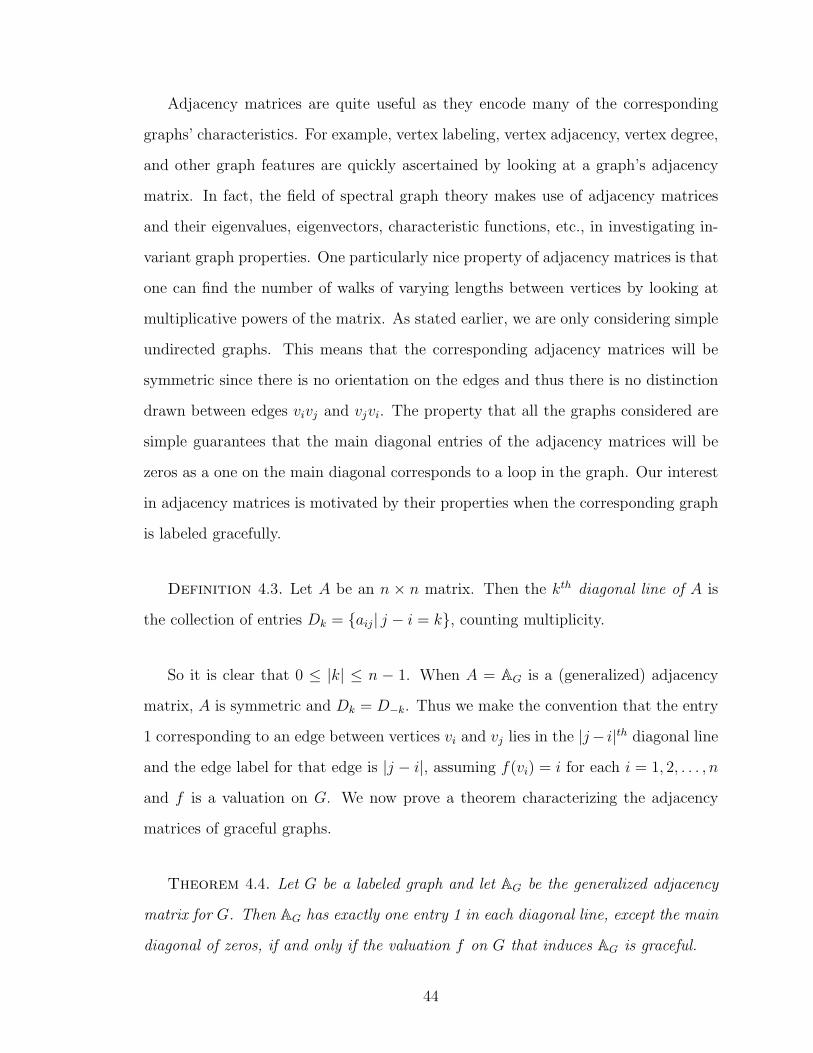
Example 4.5. We now consider the caterpillar shown in Figure 4.1 below. This
1 13
7 12
8 11 10
9
6162
317
4 14
15
5
113 7
12 8
11 10 9 616 2
3
4
14
15
5
Figure 4.1: A Graceful Caterpillar
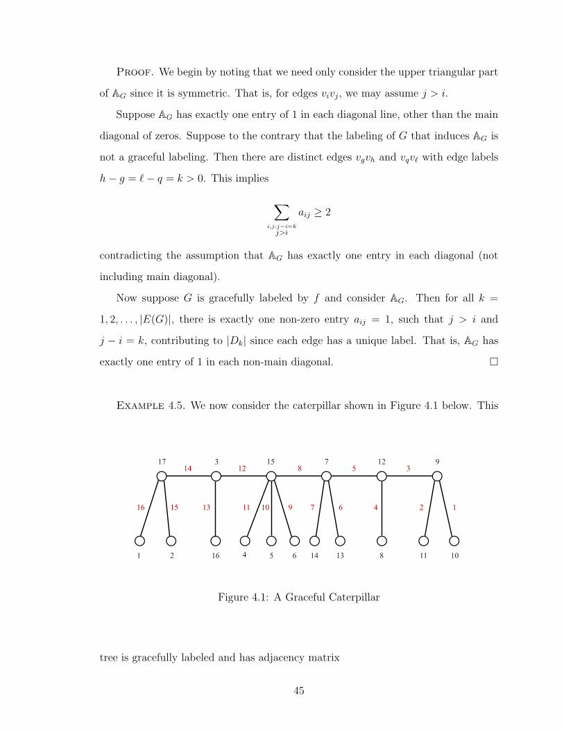
tree is gracefully labeled and has adjacency matrix
45
0 0 0 0 0 0 0 0 0 0 0 0 0 0 0 0 10 0 0 0 0 0 0 0 0 0 0 0 0 0 0 0 10 0 0 0 0 0 0 0 0 0 0 0 0 0 1 1 10 0 0 0 0 0 0 0 0 0 0 0 0 0 1 0 00 0 0 0 0 0 0 0 0 0 0 0 0 0 1 0 00 0 0 0 0 0 0 0 0 0 0 0 0 0 1 0 00 0 0 0 0 0 0 0 0 0 0 1 1 1 1 0 00 0 0 0 0 0 0 0 0 0 0 1 0 0 0 0 00 0 0 0 0 0 0 0 0 1 1 1 0 0 0 0 00 0 0 0 0 0 0 0 1 0 0 0 0 0 0 0 00 0 0 0 0 0 0 0 1 0 0 0 0 0 0 0 00 0 0 0 0 0 1 1 1 0 0 0 0 0 0 0 00 0 0 0 0 0 1 0 0 0 0 0 0 0 0 0 00 0 0 0 0 0 1 0 0 0 0 0 0 0 0 0 00 0 1 1 1 1 1 0 0 0 0 0 0 0 0 0 00 0 1 0 0 0 0 0 0 0 0 0 0 0 0 0 01 1 1 0 0 0 0 0 0 0 0 0 0 0 0 0 0
which satisfies Theorem 4.4. In fact, it is easy to see that the labeling described in
Theorem 4.4 will always give a “staircase shaped” matrix.
The condition from Theorem 4.4 allows us to look at an adjacency matrix and
immediately determine if the graph is labeled gracefully. We now consider several
families of trees that can be shown to be graceful by building the adjacency matrix
to be graceful.
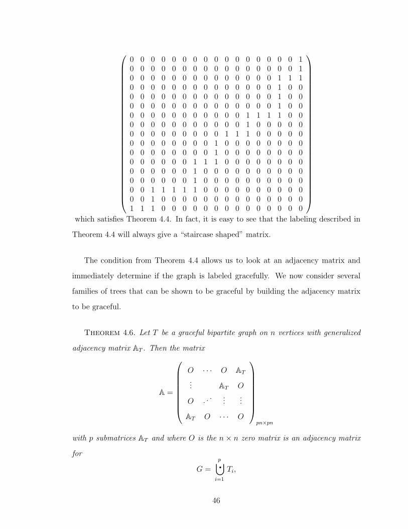
Theorem 4.6. Let T be a graceful bipartite graph on n vertices with generalized
adjacency matrix AT . Then the matrix
A =
O · · · O AT
... AT O
O . . . ......
AT O · · · O
pn×pn
with p submatrices AT and where O is the n× n zero matrix is an adjacency matrix
for
G =
p·⋃i=1
Ti,
46
the disjoint union of p copies of T .
Here we pause to note that all trees are bipartite. Thus this theorem holds for
graceful trees.
Proof. We begin by noting that A is a (0,1)-matrix, and since AT is symmetric,
so is A. Also, the main diagonal of A has all zero entries. This can be seen by the
fact that the main diagonal does not contain entries from any submatrix AT when
p is even, and goes through exactly the main diagonal of one of the AT when p is
odd. So A is a generalized adjacency matrix. We now want to show that it is the
generalized adjacency matrix for G = ·∪Ti, i = 1, 2, . . . , p.
Consider V (T ). Note that if AT is graceful, then there is an edge with induced
label m. Thus, there are adjacent vertices with labels 1 and m + 1. Let x ∈ V (T )
be the vertex such that f(x) = 1 where f is the graceful valuation of T . Since T is
bipartite, we can fix a bipartition V1, V2 of the vertices such that x ∈ V1. Moreover,
{v ∈ V (T )|d(x, v) is even } ⊆ V1 and {v ∈ V (T )|d(x, v)is odd } ⊆ V2, with equality
holding if T is connected. Also, in the generalized adjacency matrix AT of the graph
T , we have that aij = 1 implies that vi ∈ V1 and vj ∈ V2 or vice versa. We will denote
by C and D the set of labels on vertices of V1 and V2. That is,
C = {` : v` ∈ V1} and
D = {` : v` ∈ V2}
Now consider the p copies of AT in the generalized adjacency matrix A. We will call
a copy the j-th copy if it is the j-th counting from the bottom left corner of A.
For a set of integers S, let a+ S = {a+ s|s ∈ S} for any a ∈ Z. It is easy to see
that for j ∈ {1, 2 . . . , p} the j-th copy of AT in A defines edges between vertices with
labels ((j − 1)n+ C
)∪((p− j)n+D
),
47
and there is an edge v(j−1)n+iv(p−j)n+` for some i ∈ C and ` ∈ D precisely when
vi ∈ V1, v` ∈ V2 and vivj ∈ E(T ). Thus, the j-th copy of AT induces an isomorphic
copy Tj of T on the corresponding vertex set. It is easy to see that the Tj are vertex
disjoint. �
There are a few things we wish to note about the matrix constructed in Theorem
4.6. First off, since AT is the generalized adjacency matrix of a graceful graph, each
diagonal line of A has at most one 1. In fact, the only diagonal lines with all zero
entries are the diagonal lines Dk, with k = 0,±n,±2n, . . . ,±(p−2)n,±(p−1)n. This
means that the edge labels for the edges of G are distinct though not all labels from
{1, 2, . . . , pn− 1} are used.
Definition 4.7. Let G1 and G2 be two bipartite graphs with m = ||G1|| =
||G2||. Let f1 and f2 be labelings of G1 and G2 from the set {1, 2, . . . ,m + 1},
respectively. We call f1 and f2 compatible labelings, if there are disjoint sets C,D,
where C ∪ D = {1, 2 . . . ,m+ 1} and bipartitions (C1, D1) of G1, (C2, D2) of G2 such
that f1(C1), f2(C2) ⊆ C and f1(D2), f2(D2) ⊆ D. It follows that isomorphic graphs
are easily seen to be compatible.
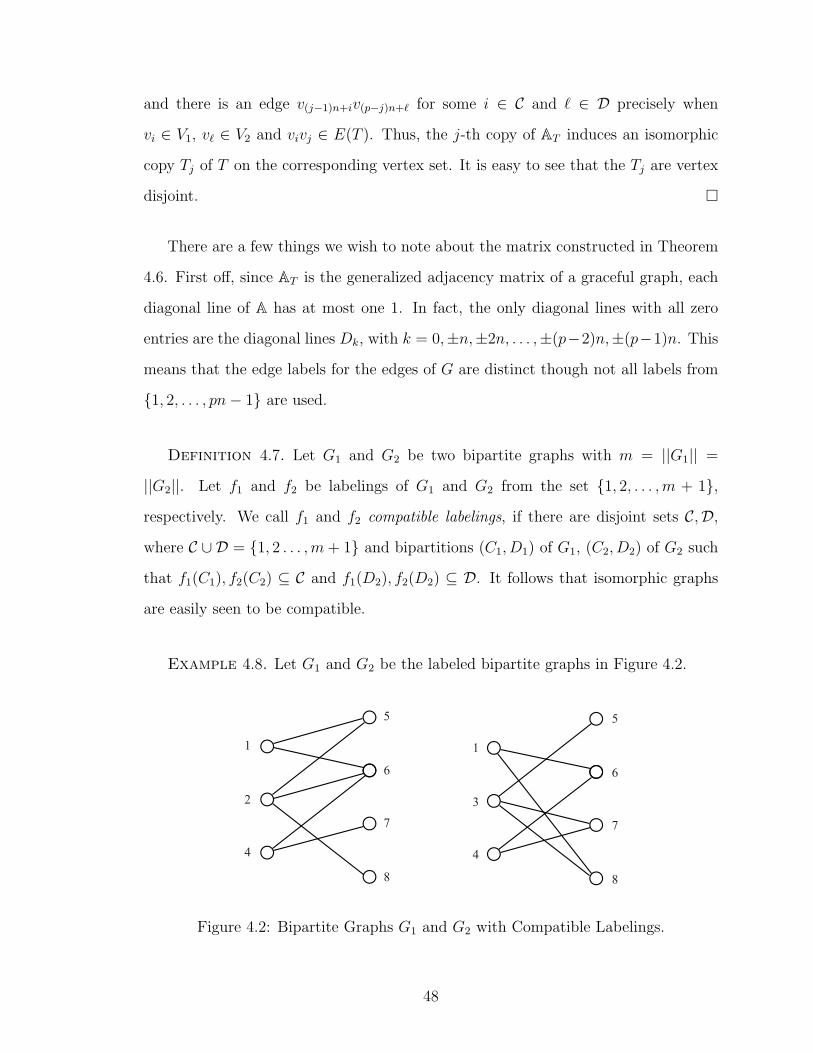
Example 4.8. Let G1 and G2 be the labeled bipartite graphs in Figure 4.2.
1
2
4
5
6
7
8
1
3
4
5
6
7
8
Figure 4.2: Bipartite Graphs G1 and G2 with Compatible Labelings.
48
Then clearly the labelings of G1 and G2 are compatible labelings. Note, however,
that these labelings are not graceful.
Theorem 4.9. Let T1, T2, . . . , Tp be graceful bipartite graphs such that Ti and
Tp+1−i have compatible graceful labelings, and denote the generalized adjacency ma-
trices of these compatible labelings by ATi. Then the matrix
A =
O · · · O ATp
... ATp−1 O
O . . . ......
AT1 O · · · O
pn×pn
with p submatrices of the form ATiand where O is the n×n zero matrix is a generalized
adjacency matrix for
G =
p·⋃i=1
Ti,
the disjoint union of vertex-disjoint copies of T . Note that if T is a tree, then A is
the usual adjacency matrix of G.
The proof of this theorem is essentially the same as that of the previous theorem,
thus we omit it.
Let T be a graceful tree on n vertices with valuation f . We want to construct a
new tree by identifying a leaf of K1,p with the vertex x such that f(x) = 1 in each
of p copies of T . We denote this tree by T ◦ K1,p. It has been shown that the tree
constructed this way, previously called T pv , is graceful in Theorem 3.22. The next
definition gives us a way to describe the graph resulting from matrix manipulations.
Definition 4.10. The matrix A is said to gracefully induce G if A is an adjacency
matrix for G, and A satisfies the conditions of Theorem 4.4.
Theorem 4.11. Let T be a graceful tree on n vertices. Then the graph T ◦K1,p
is graceful.
49
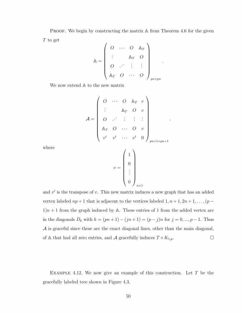
Proof. We begin by constructing the matrix A from Theorem 4.6 for the given
T to get
A =
O · · · O AT
... AT O
O . . ....
...
AT O · · · O
pn×pn
.
We now extend A to the new matrix
A =
O · · · O AT v
... AT O v
O . . ....
......
AT O · · · O v
vt vt · · · vt 0
pn+1×pn+1
.
where
v =
1
0
...
0
n×1
and vt is the transpose of v. This new matrix induces a new graph that has an added
vertex labeled np+ 1 that is adjacent to the vertices labeled 1, n+ 1, 2n+ 1, . . . , (p−
1)n + 1 from the graph induced by A. These entries of 1 from the added vertex are
in the diagonals Dk with k = (pn+ 1)− (jn+ 1) = (p− j)n for j = 0, ..., p− 1. Thus
A is graceful since these are the exact diagonal lines, other than the main diagonal,
of A that had all zero entries, and A gracefully induces T ◦K1,p. �
Example 4.12. We now give an example of this construction. Let T be the
gracefully labeled tree shown in Figure 4.3.
50
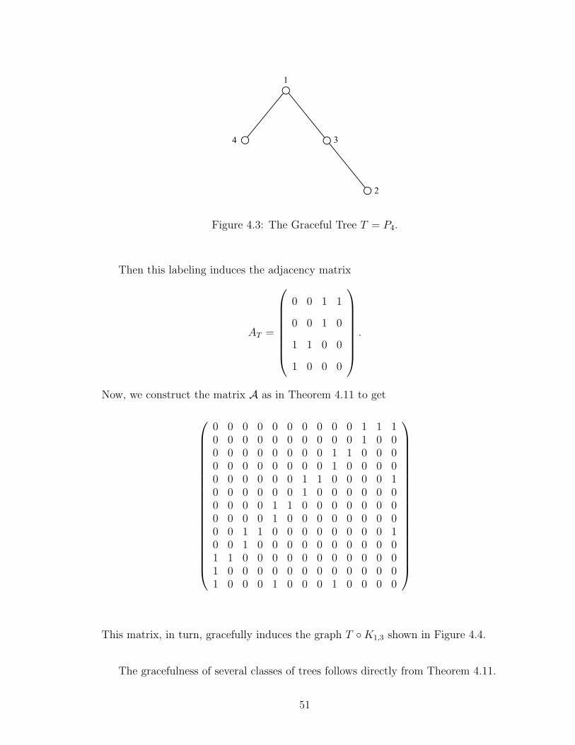
1
4
2
3
Figure 4.3: The Graceful Tree T = P4.
Then this labeling induces the adjacency matrix
AT =
0 0 1 1
0 0 1 0
1 1 0 0
1 0 0 0
.
Now, we construct the matrix A as in Theorem 4.11 to get
0 0 0 0 0 0 0 0 0 0 1 1 10 0 0 0 0 0 0 0 0 0 1 0 00 0 0 0 0 0 0 0 1 1 0 0 00 0 0 0 0 0 0 0 1 0 0 0 00 0 0 0 0 0 1 1 0 0 0 0 10 0 0 0 0 0 1 0 0 0 0 0 00 0 0 0 1 1 0 0 0 0 0 0 00 0 0 0 1 0 0 0 0 0 0 0 00 0 1 1 0 0 0 0 0 0 0 0 10 0 1 0 0 0 0 0 0 0 0 0 01 1 0 0 0 0 0 0 0 0 0 0 01 0 0 0 0 0 0 0 0 0 0 0 01 0 0 0 1 0 0 0 1 0 0 0 0
This matrix, in turn, gracefully induces the graph T ◦K1,3 shown in Figure 4.4.
The gracefulness of several classes of trees follows directly from Theorem 4.11.
51
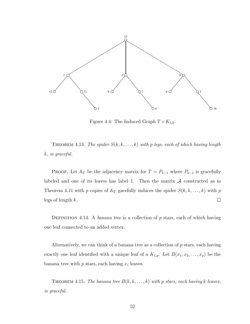
5
8
6
7
1
12
2
11
9
4
10
3
13
Figure 4.4: The Induced Graph T ◦K1,3.
Theorem 4.13. The spider S(k, k, . . . , k) with p legs, each of which having length
k, is graceful.
Proof. Let AT be the adjacency matrix for T = Pk−1 where Pk−1 is gracefully
labeled and one of its leaves has label 1. Then the matrix A constructed as in
Theorem 4.11 with p copies of AT gacefully induces the spider S(k, k, . . . , k) with p
legs of length k. �
Definition 4.14. A banana tree is a collection of p stars, each of which having
one leaf connected to an added vertex.
Alternatively, we can think of a banana tree as a collection of p stars, each having
exactly one leaf identified with a unique leaf of a K1,p. Let B(x1, x2, . . . , xp) be the
banana tree with p stars, each having xi leaves.
Theorem 4.15. The banana tree B(k, k, . . . , k) with p stars, each having k leaves,
is graceful.
52
Proof. Let AT be the adjacency matrix for T = K1,k where K1,k is gracefully
labeled and one of its leaves is labeled 1. Then the matrix A constructed as in
Theorem 4.11 with p copies of AT gracefully induces B(k, k, . . . , k). �
It is beyond the scope of this thesis to elaborate much more on graceful trees,
though certainly there is plenty more that can be said. Therefore, we end here and
refer the interested reader to Gallian’s A Dynamic Survey of Graph Labelings [5] for
a comprehensive treatment of the Graceful Tree Conjecture.
53
Bibliography
1. R. E. L. Aldred and B. D. McKay, Graceful and Harmonious Labellings of Trees,Bulletin of the Institute of Combinatorics and its Applications, 23 (1998), 69-72.
2. M. Burzio and G. Ferrarese, The Subdivision Graph of a Graceful Tree is a GracefulTree, Discrete Mathematics, 181 (1998) No. 1-3, 275-281.
3. I. Cahit, Are All Complete Binary Trees Graceful?, American MathematicsMonthly, 83 (1976), 35-37.
4. G. Chartrand and P. Zhang, Introduction to Graph Theory, McGraw Hill, NewYork (2005).
5. J. A. Gallian, A Dynamic Survey of Graph Labeling The Electronic Journal ofCombinatorics, (http://www.combinatorics.org/) DS6 16 (2009).
6. S. W. Golomb, How to Number a Graph, Graph Theory and Computing, R. C.Read, Editor, Academic Press, New York (1972), 23-37.
7. F. Harary, The Four-Color Conjecture and Other Graphical Diseases, Proof Tech-niques in Graph Theory, Academic Press, New York (1969), 1-9.
8. P. Hrnciar and A. Haviar, All Trees of Diameter Five are Graceful, Discrete Math-ematics, 233 (2001), 133-150.
9. C. Huang, A. Kotzig, A. Rosa, Further Results on Tree Labelings, Utilitas Math-ematica, 21 (1982), 31-48.
10. K. M. Koh, D. G. Rogers, T. Tan, Interlaced Trees: A Class of Graceful Trees,Combinatorial Mathematics, VI, 1978, pp. 65-78 Lecture Notes in Mathematics,748, Springer, Berlin, 1979.
11. K. M. Koh, D. G. Rogers, T. Tan, On Graceful Trees, Nanta Mathematica, 10(1977) No. 2, 207-211.
12. K. M. Koh, D. G. Rogers, T. Tan, Two Theorems on Graceful Trees, DiscreteMathematics, 25 (1979) No. 2, 141-148.
54

13. D. G. Rogers, A Graceful Algorithm, Southeast Asian Bulletin of Mathematics,2 (1978), 42-44.
14. A. Rosa, Labelling Snakes, Ars Combinatorica, 3 (1977), 67-73.
15. A. Rosa, On Certain Valuations of the Vertices of a Graph, Theory of Graphs (In-ternational Symposium, Rome, July 1966), Gordon and Breach, N.Y. and DunodParis (1967), 349-355.
16. W. D. Wallis, A Beginner’s Guide to Graph Theory, Birkhauser, Boston (2007),p. 125.
17. S. L. Zhao, All Trees of Diameter Four are Graceful, Graph Theory and its Appli-cations: East and West (Jinan, 1986), 700-706, Annals of the New York Academyof Sciences, 576, New York Academy of Sciences, New York, 1989.
55