1

Gravity Equations and Economic Frictions in the World Economy by Jeffrey H. Bergstrand and Peter Egger At the same time that the modern theory of international trade due to comparative advantage

developed in the post-World War II era to explain the patterns of international trade using 2x2x2 general

equilibrium models, a small and separate line of empirical research in international trade emerged to

“explain” statistically actual aggregate bilateral trade flows among large numbers of countries. Drawing

upon analogy to Isaac Newton’s Law of Gravitation, these international trade economists noted that

observed bilateral aggregate trade flows between any pair of countries i and j could be explained very

well using statistical methods by the product of the economic sizes of the two countries (GDPiGDPj)

divided by the distance between the country pairs’ major economic centers (DISTij). Specifically, these

researchers conjectured that:

PXij= β0(GDPi)β1(GDPj)β2(DISTij)β3 εij (1)

or

lnPXij= lnβ0 + β1lnGDPi + β2lnGDPj + β3lnDISTij +ln εij

(2)

where PXij is the value (in current prices) of the merchandise trade flow from exporter i to importer j,

GDPi (GDPj) is the level of nominal gross domestic product in country i (j), DISTij is the bilateral

physical distance between the economic centers of countries i and j, and εij is assumed to be a log-

normally distributed error term. In equation (2), ln refers to the natural logarithm. Intuition suggested that

β1 >0, β2 > 0, and β3 < 0. In the 1960s, equations (1) and (2) came to be known among international trade

economists as the “gravity equation” – owing to its obvious similarity to Newton’s gravity equation in

physics. Two notable aspects of equations (1) or (2) were that (i) actual bilateral trade flows could be

explained quite well by this specific and simple multiplicative or log-linear equation and (ii) bilateral

trade flows were actually strongly influenced by economic trade “frictions” (or trade “costs”) – such as

2

distance – which had played a very minor role in the traditional theory of international trade.1

This chapter examines both the role of frictions in international trade and the contribution of the

gravity equation toward understanding international trade flows. The gravity equation has also been used

extensively for understanding the determinants of observed bilateral foreign direct investment and

migration flows, although to an extent less than for trade flows; we will address these flows also but not

as extensively, due to space constraints. We organize our chapter into 5 parts. Section 1 discusses the

role of frictions inhibiting the flows of goods, services, capital, and labor in the world economy. While

distance has long been recognized as a prominent friction impeding trade, foreign direct investment

(FDI), and migration flows, there are numerous other impediments to these flows, some of which are also

“natural” – such as being landlocked – and some of which are “un-natural” (or “man-made”) – such as

government-policy-based impediments. In the remainder of the paper, we discuss the gravity equation.

Section 2 discusses the historical evolution of the literature on and contribution of the “traditional”

gravity equation, including some important empirical applications. However, starting in 1979, rigorous

theoretical general equilibrium foundations surfaced for the gravity equation for trade. Section 3

discusses the state-of-the-art in theoretical foundations for the gravity equation for trade and econometric

implications of these developments since 1979. Yet, in a world with multinational enterprises,

international trade flows are not independent of FDI and migration flows. Section 4 discusses very recent

developments in the theoretical foundations for the gravity equation in a world with national and

multinational firms, and econometric implications of these developments for understanding trade, FDI,

and migration flows. Section 5 concludes.

1. Frictions in the World Economy

Contrary to the popular notion that globalization has proceeded so rapidly due to technological

advance and trade-policy liberalizations, frictions to international trade, FDI, and migration flows are still

prominent and play an important role in explaining the levels of such flows. Part A discusses important

frictions to international trade flows. Part B discusses frictions to FDI flows. Part C discusses those

1A common measure of a good statistical fit is the R2 measure. Gravity equations often produced R2 values

of 80-90 percent. This suggests that 80-90 percent of the variation across country pairs in observed trade flows could be explained the variation in GDPs and bilateral distance (using the logarithmic version in ordinary linear least

3

frictions associated with migration flows.

A. Trade Frictions

Frictions that impede international trade flows are often called “trade costs.” Trade costs can be

decomposed into two main sources: “natural” trade costs and “unnatural” (or policy-based) trade costs.

Natural trade costs refer to those costs incurred largely – though not exclusively – by geography.

Distance between a pair of countries is an example of a natural trade cost. Unnatural trade costs refer to

those additional costs impeding trade if physical distances (or other natural costs) were absent. These

costs are largely “man-made” or “artificial,” and are mainly attributable to policy decisions of

governments. A tax imposed by one nation’s (j’s) government on imports from another country (i) –

typically called a tariff – is an example of a policy-based (or man-made) trade cost.

1. Natural Trade Frictions

Natural trade costs can be decomposed into transport costs and other related costs. The most

common measure of transport costs is referred to commonly as the “cif-fob factor.” Trade flows from one

country to another are often measured “free on board” (fob), which refers to the value of a shipment of

goods delivered to and put “on board” an overseas vessel for potential shipment. The same trade flows

are often also measured reflecting “cost-insurance-freight” (cif), which refers to the value of the same

shipment at the destination port (or airport), including the cost of insurance and freight charges. The ratio

of these two values minus unity provides an ad valorem “rate” for the add-on associated with

international transport. Baier and Bergstrand (2001) report that average cif-fob factors for 16

Organization for Economic Co-operation and Development (OECD) countries in 1958 and 1988 were 8.2

percent and 4.3 percent, respectively. Moreover, they show that the decline in such costs explain about 8

percent of the increase in world trade from the late 1950s to the late 1980s, after accounting for expanding

GDPs and falling tariffs. Hummels (1999) finds that freight rates in 1994 vary dramatically across

countries with average transport costs ranging from 3.8 percent for the United States to 13.3 percent for

land-locked Paraguay. Such costs vary even more across commodities within countries. An excellent

early study defining the major issues with respect to cif-fob measurements is Moneta (1959). Data on cif-

squares (OLS)).

4

fob factors is obtainable from the International Monetary Fund, either through the International Financial

Statistics or the Direction of Trade Statistics.

Intuitively, one would expect that geographic variables – such as distances between two

countries’ economic centers and sharing a common land border (often termed in the literature

“adjacency”) – would be important factors explaining trade costs; such intuition is correct, although other

factors matter as well. Two excellent studies that have examined systematically the geographic (and

miscellaneous) factors explaining variation in cif-fob factors (and other measures of shipping costs) are

Hummels (1999) and Limão and Venables (2001). Hummels (1999) finds robust evidence that the

transport-cost factor’s elasticity with respect to distance is approximately 0.25; this implies a 4 percent

increase in distance raises the transport-cost factor by 1 percent. Hummels (2007) found that fuel costs

matter also in explaining transport-cost factors.

Limão and Venables (2001) also examined the determinants of transport-cost factors. Using a

unique data set on shipments from Baltimore, Maryland in the United States to various destinations and

also using cif-fob factors to over 100 countries, these authors found that transport-cost factors were

influenced by both marginal and fixed cost factors. Regarding marginal costs, Limão and Venables

(2001) found that the distance between and adjacency of two countries had economically and statistically

significant effects on transport-cost factors, with distance increasing costs and adjacency (representing

better transit networks) reducing costs. Regarding fixed trade costs, the authors found that – for coastal

economies – the higher the level/quality of infrastructure of both the exporting and importing countries

the lower the cost, and – for landlocked countries – the higher the level or quality of infrastructure of the

“transit” exporting or importing country (the one used for its ocean port) the lower the cost. Since the

level of infrastructure in economies is endogenous to the level of government expenditures, and

consequently infrastructure may be considered a “policy-based” factor by some researchers.

While cif-fob factors are the most common method for estimating the costs associated with transit

of a good from country i to country j, this measure is not without flaws. Hummels (2007) raises the

concern that this measure may underestimate the true transport costs. He finds that the average level (and

variances) of cif-fob factors in disaggregated data is much higher than that in aggregate data. He

5

interprets the lower cif-fob factors for aggregate data as reflecting that importers minimize transport costs;

thus, trade costs have an allocative effect on trade flows.

Time also is a natural trade cost. It takes longer on average for the same good to move between

countries than within countries (of course, it could take longer for a good to move between two cities in

the United States than between Brussels, Belgium and Amsterdam, the Netherlands). Hummels (2001)

found that every additional day in ocean travel for a shipment to arrive reduces the probability of

outsourcing manufactures by 1 percent. Moreover, he found that, conditional upon shipping, firms are

willing to pay approximately 1 percent more for a shipment for each day saved in ocean shipping.

Declines in air-shipment costs relative to ocean-shipment costs have likely increased the relative share of

of shipments by air versus ocean over the last 40 years.

The level and quality of communications in and between countries also plays a role in enhancing

trade. Goods must move within countries often to reach a port (although this is less essential as air

shipment increasingly replaces ocean transport). Anderson and van Wincoop (2004), in a comprehensive

discussion of trade costs, estimate that the average cost of delivering a good from the point of

manufacture to the destination (including international tariff and non-tariff policy barriers) is about a 170

percent add-on to the cost of producing the good. They decompose this into 74 percent international trade

costs (21 percent natural and 44 percent international-border-related) and 55 percent associated with

domestic retail and wholesale distribution costs. Also, Limão and Venables (2001) remind us that many

countries are landlocked, imposing additional costs to international trade.

2. Unnatural Trade Frictions

Unnatural trade costs refer to those costs associated with policy (hence, artificial or man-made

costs). Unnatural trade costs can be decomposed into the exhaustive categories of “tariffs” – taxes on

goods crossing international borders – and “nontariff barriers” on international trade.2 Nontariff barriers

refer to such restrictions on trade associated with customs procedures as well as “behind-the-border”

2Recently, international economists have been replacing the term nontariff “barriers” with nontariff

“measures” (where the latter can be interpreted as either impeding or aiding international trade flows); thus, some nontariff measures impose additional trade costs whereas others reduce such costs. Also, some economists consider nontariff measures to apply to non-price, non-quantity measures (thus, excluding quantitative “quotas”); however, we will consider nontariff measures to include “quotas.”

6

measures such as domestic laws and regulations that alter international relative to domestic trade.

Tariffs on goods that flow across national borders – essentially, border taxes – as a means of

protection have a long history in international trade. Due to numerous rounds of reductions in tariff rates

of developed and developing countries first under the Generalized Agreement on Tariffs and Trade

(GATT), then under the World Trade Organization (WTO), and more recently due to the spread of

regional economic integration agreements (EIAs), levels of tariffs are much lower now than, say,

immediately after World War II. Because several other earlier chapters in this handbook on trade policy

deal with tariffs in considerable detail, we need not explore the rationale for tariffs in detail here.

However, tariffs still play a considerable role in explaining trade flows empirically using the gravity

equation (to be discussed later), so some discussion of their measurement is important here. Systematic

data on bilateral tariff rates has been difficult to obtain until fairly recently. The best source for a broad

range of bilateral tariff rates by industrial sector and pairs of countries is the World Integrated Trade

Solution (WITS), available at the World Bank website. This data set reports tariff rates for developed

countries that are generally less than 5 percent. For developing countries, average tariff rates range

between 10 to 25 percent.

While measures of tariff rates are available, nontariff barriers (or measures, NTBs) are even more

difficult to quantify. One method of measurement of the importance of NTBs is to calculate the share of

industries in a country that are subject to NTBs in that country; this is typically referred to as the “NTB

coverage ratio.” Using a broad definition, it ranges from 10 percent to 75 percent, cf., Anderson and van

Wincoop (2004, Table 3). Such ratios have been used frequently in gravity equations to estimate the

impact of NTBs on trade flows, cf., Lee and Swagel (1997).

B. Frictions to Foreign Direct Investment

While empirical researchers have often been frustrated by the absence of systematic and

comprehensively constructed data sets on tariff rates and NTBs on goods trade, data for foreign direct

investment (FDI) frictions are even worse. As with goods, a useful decomposition of FDI frictions is

natural and unnatural frictions. In empirical analysis, researchers have often found bilateral distance to be

a significant impediment to bilateral FDI flows. This result has tended to raise questions about the

7

economic interpretation of distance. For many years, distance was considered to be a proxy for transport

costs. However, most trade and FDI flows – which are among developed countries – tend to be viewed as

substitutes. If distance between two countries is high, then trade costs are high, and exports (and

exporting firms) should diminish, with multinational firms replacing them and FDI increase (cf.,

Markusen, 2002); hence, distance and FDI would be positively related. However, distance and FDI are

negatively related in the data, suggesting that distance is likely reflecting trade and FDI “costs” different

from transport costs. A common interpretation of distance’s role as an impediment to trade and FDI is

that distance captures information costs.

Since a consistently negative effect of distance on FDI flows has been found, other factors

influencing information flows have been sought. As for trade flows, many studies have used binary

indicator (dummy) variables capturing the presence or absence of a common language to explain FDI

flows with success; a common language reduces information costs.

Policy variables also influence FDI frictions. One of the most common policy variables

examined that potentially influence FDI is tax policy. Higher taxes on corporate profits in host countries

have long been argued to reduce FDI; however, evidence is mixed on tax rates’ effects on FDI. See

Swenson (1994) and Desai et al. (2004) for some recent representative studies.

Another important policy variable influencing FDI behavior is tariff rates on goods. Since tariffs

on goods impose a tax on imports, firms in exporting countries may switch their provision of goods to

production in the foreign market via FDI. Consequently, tariffs may increase FDI; this is called “tariff-

jumping.” Both Belderbos (1997) and Blonigen (2002) find evidence of tariff-jumping FDI.

C. Migration Frictions

As with trade and FDI flows, natural and un-natural frictions also impede migration flows. The

literature on impediments to migration is also broad; migration issues are addressed more fully in the

chapter by Gaston and Nelson. Among natural impediments, bilateral distance, of course, plays a

significant role. Most studies of migration find that distance has an economically significant effect on

such flows. Being a landlocked country reduces migration flows significantly. The presence of a

common language has a significant effect on reducing migration costs. Also, immigrants are aided

8

significantly by a large stock of previous migrants into the destination country, as the latter provide an

infrastructure that reduces the costs to migrants of establishing themselves, cf., Hatton and Williamson

(2002, 2005). Policies also play a significant role in that most countries have quotas on the number of

immigrants and other selection policies to determine the economic characteristics of immigrants. For

more on the policy debate, see Borjas (1994, 1999), Freeman (1996), Hatton and Williamson (2002,

2005), Hanson (2006), and Grogger and Hanson (2008).

2. Historical Roots of the Gravity Equation

In this section, we discuss the literature concerning historical gravity equations of international

trade. The gravity equation actually has quite a rich history in social science applications, dating back to

the 19th century. Section A provides a brief general overview of the traditional gravity equation and

discusses the early social science roots of it.

The empirical literature on the gravity equation for international trade began in earnest around

1962, as discussed in Section B; from 1962 to 1979, the “traditional” gravity equation (2) became more

popular. In international trade, the gravity equation primarily surfaced as a statistical model to “explain”

variation in aggregate bilateral trade flows among pairs of countries for cross-sections using OLS.

A. Overview and Early Social Science Roots

The empirical explanation and prediction of interregional commodity or factor flows has been

captured for over 100 years by the gravity equation.3 Consequently, the social science literature

addressing the gravity equation is enormous. Hence, we narrow our discussion to approaches relevant

primarily to international trade flows, with some reference to FDI flows and only minimal reference to

migration flows (owing to the vastness of the migration literature).

The naming of equation (1) as the “gravity equation” in the social sciences descends, according to

Olsen (1971), from the “social physics school” at Princeton University. John Q. Stewart, a school

member who familiarized the school’s name, “found it rewarding to regard members of a social group as

the individual molecules of a physical mass and to analyze the interaction between social groups in the

same way as the physicists analyze interaction between masses” (Olsen, 1971, p. 14). In fact, Stewart

3See, for instance, Carey (1865) and Ravenstein (1885, 1889).

9

(1948) noted that a gravity equation is more closely related to Newton’s equation for the energy between

two masses, rather than its force; force is related to the inverse of the square of bilateral distance, while

energy is related to the inverse of distance (with an exponent of unity). This led Stewart to formalize

demographic “energy” into the equation:

Eij= β0(POPi)(POPj)/(DISTij) (3)

where Eij is the “demographic energy” between two countries i and j and POPi (POPj) is the population in

i (j). Equation (3) is interesting because – much later – most international trade applications have found

empirically that the elasticities of trade flows with respect to GDPs (bilateral distance) are approximately

1 (-1), as equation (3) suggests. While there has been no meta-analysis of GDP elasticities, Disdier and

Head (2008) using a meta-analysis of distance elasticities for trade flows found that the average elasticity

is -0.9.

Stewart’s “social physics school” is often considered the motivating force behind the

development of the spatial interaction/regional science literature in the 1950s, cf., Sen and Smith (1995).

For the purposes ultimately of understanding the international trade flow literature on the gravity

equation, it is useful to know that this school diverged into two fundamental paths. Sen and Smith (1995)

call one the “Deterministic Approach” and the other the “Probabilistic Approach.”

Deterministic Approaches

For international trade, economists have largely followed the Deterministic Approach. In the

“spatial interaction” literature, this approach was used as a foundation for one theory for explaining

commodity trade flows. Niedercorn and Moorehead (1974, N-M) assumed the existence of a firm

(monopolist) k in region i maximizing total revenue subject to a constraint embodying an assumption that

the firm’s total transportation cost budget and total output are fixed. The firm, according to N-M, faces

the problem of how to allocate its given total product over N different markets, such that revenue is

maximized for a given budget kYi. For instance, N-M assumed a logarithmic revenue function, kRi = ΣNj=1

POPj ln (kqij/ POPj) where kRi is total revenue of firm k in origin i and kqij is output sold by firm k in origin

10

i shipped to destination j. Assuming the transport budget constraint kYi = r ΣNj=1 (DISTij

α) (kqij), where r is

the exogenous cost per mile to ship firm k’s good and α is a parameter, maximizing revenue subject to the

transport budget constraint yields the following gravity equation:

qij= [(Yi)(POPj)]/[(r DISTijα)(ΣN

j=1POPj)] (4)

There are several limitations of the approach; we mention just some. First, there are several restrictive

assumptions to the approach, such as that all firms are monopolists. Second, this yields a gravity equation

with a measure of income for the origin region, but a measure of population for the destination. Third,

relative prices play no role. Fourth, as earlier, no other regions’ factors play a role (with the exception of

other regions’ populations). While restrictive in nature, “spatial interaction” models such as these were

early precursors of the modern theoretical foundations for international trade gravity equations. However,

before we explore those, we mention briefly some influential papers in the other thread of the spatial

interaction approach, that is, the “Probabilistic Approach.”

Probabilistic Approaches

This approach concerned explaining flows using a statistical methodology. While this literature

is also extensive, with regard to international trade flows one of the earliest models was Savage and

Deutsch (1960). The purpose of the paper was to generate a framework for “predicting” bilateral trade

flows, given information on multilateral trade (exports and imports). They intentionally avoided

specifying economic behavior, and referred to their model as the “null model.”

Leamer and Stern (1970) used the Savage-Deutsch model as the basis for a “theory” of the

gravity equation. In their model, the value of the trade flow from i to j was determined by:

PXij = M b pi qj g(Rij) + εij (5)

where b is the exogneous size of every transaction (a constant), M is the exogenous number of

transactions (a constant), Rij measures trade resistances (or enhancements), and pi (qj) would each be

11

determined by GDPs and populations in the respective countries. While the approach provided a

grounding for the multiplicative form of the gravity equation, it did not explain the unity elasticities for

GDPs, why populations should be included, the specification for g(), or the determinants of M or b.

Leamer and Stern (1970), however, did raise econometric concerns about heteroskedasticity in estimating

a log-linear version of gravity equation (5) by ordinary least squares, concerns that would surface

prominently more than 30 years later.

B. The Gravity Equation in International Trade: 1962 to 1979

The gravity equation -- most commonly specified as equation (2) -- became a popular tool

beginning in the early 1960s to explain actual aggregate gross bilateral trade flows. This equation did

not evolve from the mainstream theory of international trade, discussed in Part A of this volume. The

mainstream theory – and empirical evaluation of it – in the 1960s was concerned instead with explaining

the pattern and commodity composition of trade. Ricardo’s theory of comparative advantage and the

Heckscher-Ohlin model were basically silent on aggregate gross bilateral trade flows (especially in

empirical “multi-country” settings, that is, with the number of countries N exceeding 2). By contrast, the

study of aggregate gross bilateral trade flows has been referred to as the analysis of the “volume” of trade.

In the international trade literature, Nobel laureate Jan Tinbergen is credited as the first to specify

econometrically what has become a benchmark “traditional” gravity equation for studying international

trade flows, cf., Tinbergen (1962). Using a specification similar to equation (2), Tinbergen estimated:

lnPXij= lnβ0 + β1 lnGDPi + β2 lnGDPj + β3 lnDISTij + β4 ADJij + β5 EIA1ij + β6 EIA2ij + lnεij (6)

where ADJ, EIA1, and EIA2 are dummy variables with values of 1 if two countries share a common land

border, are members of the British Commonwealth, and are members of the BENELUX free trade

agreements, respectively (and zero otherwise).4 Tinbergen found GDP elasticities of 0.7 and 0.6 for i and

4EIA denotes “economic integration agreement.” Note that Walter Isard’s work had a substantive influence

on Tinbergen’s work, cf., Isard (1954a,b; 1960), which itself built upon the work of Stewart (1948) and Reilly (1929).

12

j, respectively, a distance elasticity of -0.6, and a small but statistically significant effect of

Commonwealth membership of 5 percent (0.05). In fact, the motivation for Tinbergen’s use of the

gravity equation was to determine the “normal pattern” of international trade in the absence of

“discriminatory trade impediments” (such as the Commonwealth or BENELUX) and to estimate the

effect of such agreements day (cf., Tinbergen, 1962, p. 262), a central motivation for using the gravity

equation to this day.

Tinbergen’s work is important also in spurring more studies by his students. Pöyhönen (1963a,

b), Pulliainen (1963), and Linnemann (1966) developed further the theoretical and empirical foundations

for the gravity equation. Especially noteworthy was Linnemann (1966), the first monograph to use the

gravity equation in an extensive empirical analysis. In international trade, many empirical applications of

the gravity equation to aggregate bilateral trade flows appealed to a third approach, an economic model

described in Linnemann (1966). The Linnemann model was based upon the following approach.

Suppose importer j’s demand for the trade flow from i to j (PXDi j) is a function of j’s GDP, the price of

the product in i (pi), and distance from i to j. Suppose exporter i’s supply of goods (PXSi) is a function of

i’s GDP and pi. Market clearing would require county i’s export supply to equal the sum of the N-1

bilateral import demands (in an N-country world). This generates a system of N+1 equations in N+1

endogenous variables: N-1 bilateral import demands PXDi j (j = 1,..., N with j≠i), supply variable PXS

i, and

price variable pi. This system could be solved for a bilateral trade flow equation for PXij that is a function

of the GDPs of i and j and their bilateral distance. Then pi is endogenous and excluded from the reduced-

form bilateral trade flow gravity equation.

There are several shortcomings of this approach; we mention a few. First, the model cannot

explain the multiplicative form of the gravity equation. Second, to eliminate all other N-2 countries’

prices, Linnemann (1966) assumed a “general world price level” due to arbitrage and perfect product

substitutability (cf., p. 41). Third, microeconomic foundations for including GDPs (and, in some studies,

populations of countries) are absent. Nevertheless, in one of the earliest survey’s of the gravity equation

in trade, Leamer and Stern (1970) considered Linnemann’s theory as one of three alternative approaches,

alongside the spatial interaction deterministic and the probability approaches.

13

Linnemann’s book provided a major breakthrough in terms of empirical analysis of aggregate

bilateral trade flows, and remains a useful resource. Among empirical contributions, Linnemann found:

(1) half of world trade flows are measured as zeros (under $100,000 technically), creating econometric

problems, an issue only addressed systematically 30 years later in Felbermayr and Kohler (2006), Santos

Silva and Tenreyro (2006), Helpman, Melitz, and Rubenstein (2008), and Egger, Larch, Staub, and

Winkelmann (2009),

(2) measurements of the “economic centers” of countries to calculate economic distance (sea and land)

for a large number of countries, used by subsequent researchers,

(3) identification of a large sample of economic integration agreements potentially causing trade creation

and diversion and the first economically and statistically significant ex post trade-creation effects of

preferential trade agreements,

(4) potential effects of heteroskedasticity identified,

(5) the first estimates suggesting that trade diversion from preferential trade agreements is quite limited.

The empirical success of Linnemann’s work led to other researchers looking to find ex post

estimates of economic integration agreements (EIAs) on trade flows. Aitken (1973) provided one of the

first sets of a time-series of cross-sections to try to estimate the effects of the original six-member

European Economic Community (EEC) and original seven-member European Free Trade Agreement

(EFTA) on trade flows. He found no economically or statistically significant effect of the agreements

prior to the date-of-entry, and economically and statistically significant effects on trade of the EEC

(EFTA) in 1963 (1966) and later years. Aitken then used coefficient estimates to generate gross and net

trade creation effects of membership for each country. Sapir (1981) used the same methodology to

estimate effects of the Generalized System of Preferences (GSP) for developing countries.

These two studies provided the first economically plausible and statistically significant effects of

EIAs on trade, providing guidance for numerous subsequent empirical analyses using the traditional

gravity equation. The traditional gravity equation was subsequently used to model the effects of

numerous other economic, political, cultural, and social variables on trade flows. For instance, Dunlevy

and Hutchinson (1999) estimate the impact of immigration flows on international trade, Abrams (1980)

14

and Thursby and Thursby (1987) the effect of exchange rate variability on trade, Rose (2000) and Frankel

and Rose (2002) the effect of currency unions on trade, Pollins (1989) and Reuveny and Kang (2003) the

effect of international political conflicts on trade, Gowa and Mansfield (1993) and Mansfield and Bronson

(1997) the effect of military alliances on trade, van Beers (1998) the effect of labor standards on trade,

and McCallum (1995) national political borders on trade; these are only a few of the numerous studies.

3. Gravity Equations of Trade Based on General Equilibrium Models: 1979 to Present

Prior to 1979, the absence of rigorous theoretical microeconomic foundations for the gravity

equation in international trade inhibited its use for policy work and left the equation on the periphery of

mainstream international trade research. Beginning in 1979, theoretical rationales for the gravity equation

in trade surfaced based upon general equilibrium frameworks. The models tended to take either of two

paths. One approach assumed “separability” of production and consumption decisions from the decision

concerning with which country to trade (henceforth, the “trade-separability” assumption). The

separability of the bilateral trade decision from production and consumption decisions implied a two-

stage budgeting process, and the gravity equation assumed an “endowment economy” to ignore the first-

stage decision regarding production and consumption in countries. These “conditional general

equilibrium” (or conditional GE) models are discussed in section A. Theoretical foundations also

surfaced in the absence of the “trade-separability” assumption. These formulations – henceforth,

“unconditional” GE models – will be addressed in section B. Finally, section C will address advances in

empirical implementations of the gravity equation.

A. Conditional General Equilibrium (GE) Approaches

Anderson (1979) is generally recognized as the first formal conditional GE model of the gravity

equation for trade. The model is based upon three assumptions. First, assume that each country

specializes completely in the production of its own good, and there is one good for each country produced

exogenously (i.e., an “endowment economy”). Second, assume identical, homothetic preferences. Third,

assume a frictionless world with zero transport costs, tariffs, and distribution costs; with no frictions, all

prices can be normalized to unity. In this world, the value of trade from i to j (PXij) can be represented by:

15

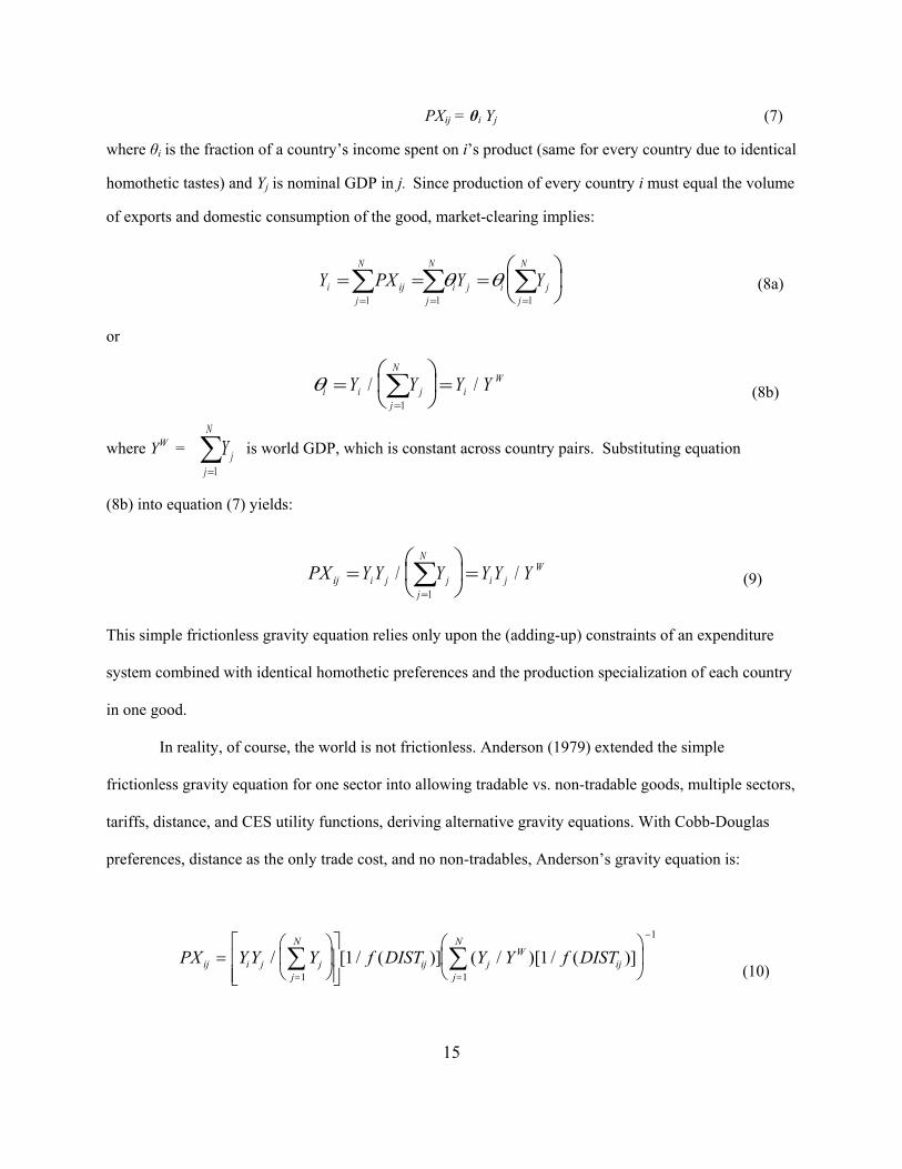
PXij = θi Yj (7)

where θi is the fraction of a country’s income spent on i’s product (same for every country due to identical

homothetic tastes) and Yj is nominal GDP in j. Since production of every country i must equal the volume

of exports and domestic consumption of the good, market-clearing implies:

(8a)

or

(8b)

where YW = is world GDP, which is constant across country pairs. Substituting equation (8b) into equation (7) yields:

(9)

This simple frictionless gravity equation relies only upon the (adding-up) constraints of an expenditure

system combined with identical homothetic preferences and the production specialization of each country

in one good.

In reality, of course, the world is not frictionless. Anderson (1979) extended the simple

frictionless gravity equation for one sector into allowing tradable vs. non-tradable goods, multiple sectors,

tariffs, distance, and CES utility functions, deriving alternative gravity equations. With Cobb-Douglas

preferences, distance as the only trade cost, and no non-tradables, Anderson’s gravity equation is:

(10)

Y PX Y Yi ijj

N

i j i jj

N

j

N

= = =⎛

⎝⎜

⎞

⎠⎟

= ==∑ ∑∑

1 11

θ θ

θi i jj

N

iWY Y Y Y=

⎛

⎝⎜

⎞

⎠⎟ =

=∑/ /

1

Y jj

N

=∑

1

PX Y Y Y Y Y Yij i j jj

N

i jW=

⎛

⎝⎜

⎞

⎠⎟ =

=∑/ /

1

PX Y Y Y f DIST Y Y f DISTij i j jj

N

ij jW

ijj

N

=⎛

⎝⎜

⎞

⎠⎟

⎡

⎣⎢⎢

⎤

⎦⎥⎥

⎛

⎝⎜

⎞

⎠⎟

= =

−

∑ ∑/ [ / ( )] ( / )[ / ( )]1 1

1

1 1

16

where f(DISTij) represents trade costs – a function of distance. This equation is close in specification to

equation (1), assuming little variation across exporters i in the third term in brackets (which is a distance

weighted measure of the economic size of the rest-of-the-world), a potential source of omitted variables

bias. One limiting aspect of equation (10) is that it is not derived from a CES utility function, which

became the norm in international trade to reflect the notion of “love of variety.” With CES preferences,

equation (10) becomes more complicated, and slightly less transparent to the popular specification of

gravity equation (1) or (2).5 A second limitation of Anderson’s approach is an assumption that all prices

are assumed unity (using the convention that “free trade prices are unity”). This assumption is fine in a

frictionless world; however, with asymmetric trade costs, prices differ across producers. These limitations

of the theory motivated subsequent theoretical refinements by others – as well as by Anderson himself.

The absence of price terms in Anderson’s gravity equation (10) above motivated another

conditional GE theory for the gravity equation in Bergstrand (1985). First, starting from a “nested” CES

utility function in an endowment economy, Bergstrand derived an import demand function for goods from

i to j, allowing the elasticity of substitution among imported goods (σ) to be different potentially from that

between imported and domestic goods, μ (i.e., two-stage allocation process). Second, motivated by the

assumption that goods are tailored to foreign markets (and incorporate increasing marginal costs of

distribution and marketing as developed in rigorous detail in Arkolakis, 2008), Bergstrand assumed that

output by exporter i is not costlessly substituted among foreign markets; in Anderson (1979), goods are

costlessly substitutable across destination markets. Representing the exporter’s allocation among markets

by a constant-elasticity-of-transformation (CET) function (the elasticity given by γ) – the production

analogue to the CES utility function – Bergstrand derived an export supply function for goods from i to j.

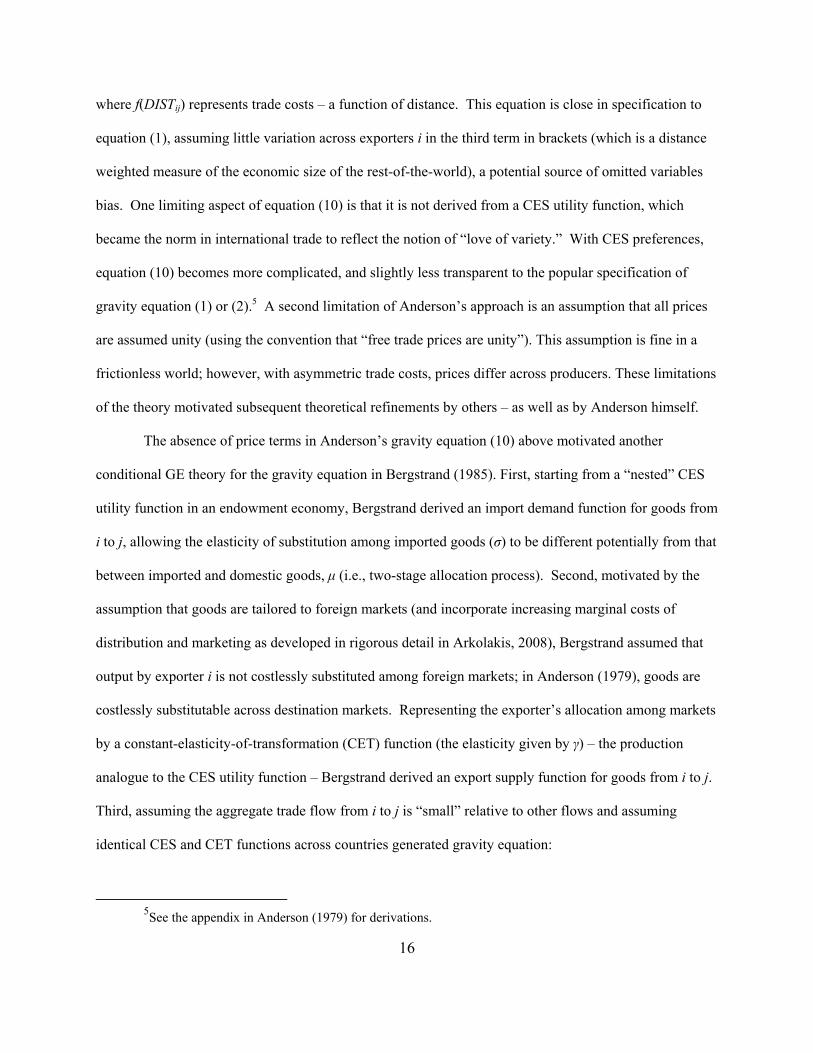
Third, assuming the aggregate trade flow from i to j is “small” relative to other flows and assuming

identical CES and CET functions across countries generated gravity equation:

5See the appendix in Anderson (1979) for derivations.

17

(11)

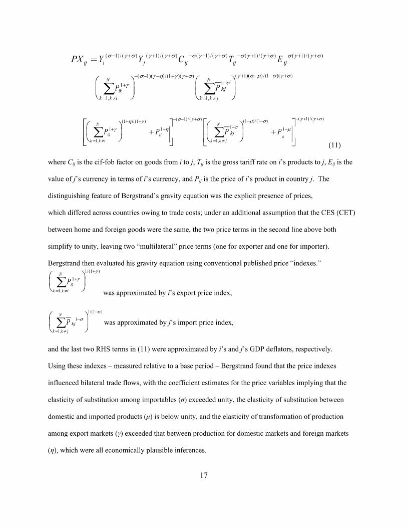
where Cij is the cif-fob factor on goods from i to j, Tij is the gross tariff rate on i’s products to j, Eij is the value of j’s currency in terms of i’s currency, and Pij is the price of i’s product in country j. The distinguishing feature of Bergstrand’s gravity equation was the explicit presence of prices, which differed across countries owing to trade costs; under an additional assumption that the CES (CET) between home and foreign goods were the same, the two price terms in the second line above both simplify to unity, leaving two “multilateral” price terms (one for exporter and one for importer). Bergstrand then evaluated his gravity equation using conventional published price “indexes.”

Pikk k i

N1

1

1 1

+

= ≠

+

∑⎛

⎝⎜

⎞

⎠⎟γ

γ

,

/ ( )

was approximated by i’s export price index,

P kjk k j

N1

1

1 1−

= ≠

−

∑⎛

⎝⎜

⎞

⎠⎟σ

σ

,

/ ( )

was approximated by j’s import price index,

and the last two RHS terms in (11) were approximated by i’s and j’s GDP deflators, respectively. Using these indexes – measured relative to a base period – Bergstrand found that the price indexes

influenced bilateral trade flows, with the coefficient estimates for the price variables implying that the

elasticity of substitution among importables (σ) exceeded unity, the elasticity of substitution between

domestic and imported products (μ) is below unity, and the elasticity of transformation of production

among export markets (γ) exceeded that between production for domestic markets and foreign markets

(η), which were all economically plausible inferences.

PX Y Y C T Eij i j ij ij ij= − + + + − + + − + + + +( ) / ( ) ( ) / ( ) ( ) / ( ) ( ) / ( ) ( ) / ( )σ γ σ γ γ σ σ γ γ σ σ γ γ σ σ γ γ σ1 1 1 1 1

P Pikk k i

N

kj

k k j

N1

1

11

1

1

+

= ≠

− − − + +−

= ≠

+ − − +

∑ ∑⎛

⎝⎜⎜

⎞

⎠⎟⎟

⎛

⎝⎜⎜

⎞

⎠⎟⎟

γ

σ γ η γ γ σσ

γ σ μ σ γ σ

,

( )( ) / (1 )( )

,

( )( ) / (1 )( )

P P P Pikk k i

N

ii kjk k j

N

jj

1

1

1 1

1

1

1

1

1 1

1

1

+

= ≠

+ +

+

− − +

−

= ≠

− −

−

− + +

∑ ∑⎛

⎝⎜

⎞

⎠⎟ +

⎡

⎣⎢⎢

⎤

⎦⎥⎥

⎛

⎝⎜

⎞

⎠⎟ +

⎡

⎣⎢⎢

⎤

⎦⎥⎥

γ

η γ

η

σ γ σ

σμ σ

μ

γ γ σ

,

( ) / ( ) ( ) / ( )

,

( ) / ( ) ( ) / ( )

18

However, cross-section empirical estimation of Bergstrand’s gravity model was compromised by

using crude indexes for multilateral price levels. GDP deflators, import price indexes, and export price

indexes measure changes in price levels relative to a base period, and consequently are much more

suitable for time-series analysis than for cross-section analysis. Since the gravity equation had typically

been used for evaluating cross-section data and long-run equilibrium relationships between trade flows

and various RHS variables, such price indexes provide only a rough approximation to their cross-

sectional values, cf., Feenstra (2004).

Up until 2003, many empirical gravity applications over the years cited the (conditional GE)

models of Anderson (1979) and Bergstrand (1985) as theoretical foundations for the gravity equation.

However, such studies usually either ignored the role of multilateral prices or included readily-available

price indexes. For instance, McCallum (1995) found that – due to the Canadian-U.S. national border –

inter-provincial Canadian trade flows were 22 times (2100 percent) higher than trade between Canadian

provinces and U.S. states, but treated multilateral prices using an ad hoc “remoteness” index.” Motivated

by McCallum (1995), Anderson and van Wincoop (2003), or A-vW, enhanced the conditional GE

theoretical foundations for estimating gravity equations, using a system of equations to allow for the

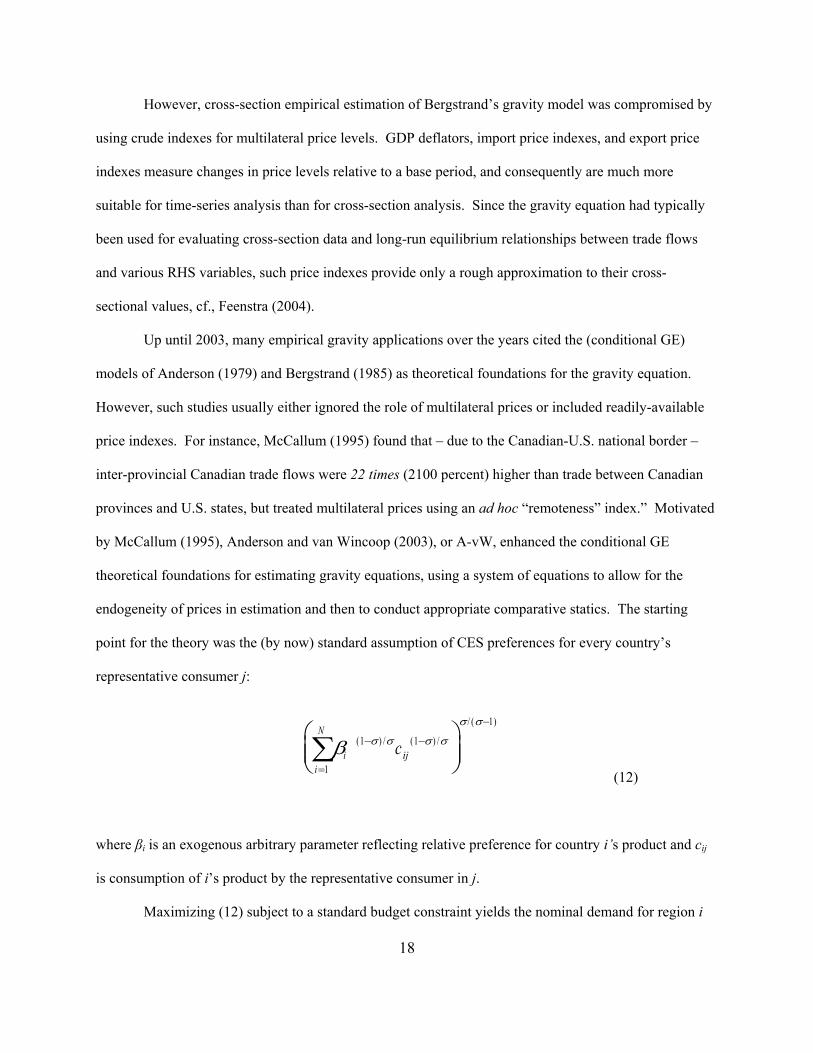
endogeneity of prices in estimation and then to conduct appropriate comparative statics. The starting

point for the theory was the (by now) standard assumption of CES preferences for every country’s

representative consumer j:

(12)

where βi is an exogenous arbitrary parameter reflecting relative preference for country i’s product and cij

is consumption of i’s product by the representative consumer in j.

Maximizing (12) subject to a standard budget constraint yields the nominal demand for region i

β σ σ σ σ

σ σ

ii

N

ijc=

− −

−

∑⎛

⎝⎜⎜

⎞

⎠⎟⎟

1

1 1

1

( ) / ( ) /

/ ( )

19

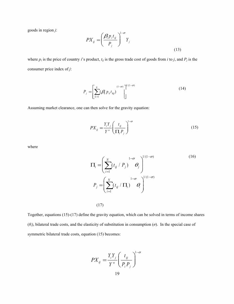
goods in region j:

(13)

where pi is the price of country i’s product, tij is the gross trade cost of goods from i to j, and Pj is the

consumer price index of j:

(14)

Assuming market clearance, one can then solve for the gravity equation:

(15)

where

(16)

(17)

Together, equations (15)-(17) define the gravity equation, which can be solved in terms of income shares

(θi), bilateral trade costs, and the elasticity of substitution in consumption (σ). In the special case of

symmetric bilateral trade costs, equation (15) becomes:

PXp tP

Yiji i ij

jj=

⎛

⎝⎜⎜

⎞

⎠⎟⎟

−β

σ1

P p tj k k kjk

N

=⎡

⎣⎢⎢

⎤

⎦⎥⎥=

− −

∑( )( ) / ( )

βσ σ

1

1 1 1

PXY YY

tPij

i jw

ij

i j

=⎛

⎝⎜⎜

⎞

⎠⎟⎟

−

Π

1 σ

Πi ij ji

N

jt P=⎛

⎝⎜⎜

⎞

⎠⎟⎟

=

− −

∑( / )

/ (1 )

1

1 1σ σ

θ

P tj ij ii

N

i=⎛

⎝⎜⎜

⎞

⎠⎟⎟

=

− −

∑( / )

/ (1 )

Π1

1 1σ σ

θ

PXY YY

tP Pij

i jw

ij

i j

=⎛

⎝⎜⎜

⎞

⎠⎟⎟

−1 σ

20

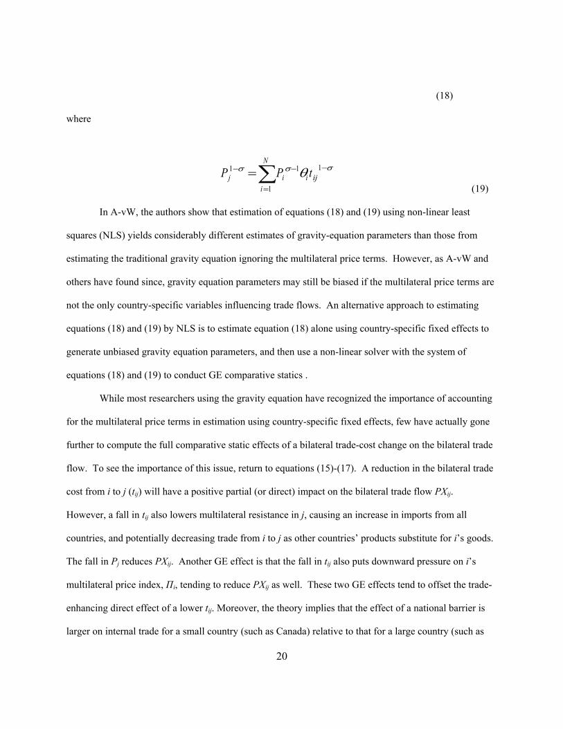
(18)

where

(19)

In A-vW, the authors show that estimation of equations (18) and (19) using non-linear least

squares (NLS) yields considerably different estimates of gravity-equation parameters than those from

estimating the traditional gravity equation ignoring the multilateral price terms. However, as A-vW and

others have found since, gravity equation parameters may still be biased if the multilateral price terms are

not the only country-specific variables influencing trade flows. An alternative approach to estimating

equations (18) and (19) by NLS is to estimate equation (18) alone using country-specific fixed effects to

generate unbiased gravity equation parameters, and then use a non-linear solver with the system of

equations (18) and (19) to conduct GE comparative statics .

While most researchers using the gravity equation have recognized the importance of accounting

for the multilateral price terms in estimation using country-specific fixed effects, few have actually gone

further to compute the full comparative static effects of a bilateral trade-cost change on the bilateral trade

flow. To see the importance of this issue, return to equations (15)-(17). A reduction in the bilateral trade

cost from i to j (tij) will have a positive partial (or direct) impact on the bilateral trade flow PXij.

However, a fall in tij also lowers multilateral resistance in j, causing an increase in imports from all

countries, and potentially decreasing trade from i to j as other countries’ products substitute for i’s goods.

The fall in Pj reduces PXij. Another GE effect is that the fall in tij also puts downward pressure on i’s

multilateral price index, Πi, tending to reduce PXij as well. These two GE effects tend to offset the trade-

enhancing direct effect of a lower tij. Moreover, the theory implies that the effect of a national barrier is

larger on internal trade for a small country (such as Canada) relative to that for a large country (such as

P P tj ii

N

i ij1 1

1

1− −

=

−=∑σ σ σθ

21

the United States), which is borne out empirically. These GE effects are the second contribution of AvW,

which helped to reduce substantively the estimated effect of the Canadian-U.S. border on international

trade between Canadian provinces and U.S. states. For instance, A-vW found that – ignoring the GE

effects – the Canadian-U.S. border reduced international trade by 80 percent. However, once GE effects

were accounted for, the border reduced Canadian-U.S. trade by only 44 percent.

While empirical researchers since (2003) have cited increasingly A-vW as theoretical foundations

for the gravity equation, and applied country fixed effects to capture the multilateral price terms in

estimation, few researchers have explored the full GE comparative static effects of trade-cost changes.6

One reason for this is the lack of effort to simulate the trade flows and multilateral price terms with and

without barriers using a non-linear solver. To offer one partial remedy for this, Baier and Bergstrand

(2009a) provided a method for “approximating” the GE comparative static effects without having to use

non-linear solvers. Baier and Bergstrand (2009a) use a first-order log-linear Taylor-series expansion of

the multilateral price terms (16) and (17) above to solve for multilateral “resistance” terms – GDP-share-

weighted (or simple) averages of the “exogenous” components of the endogenous multilateral price terms

– allowing estimation of a reduced-form gravity equation and providing a simple method to approximate

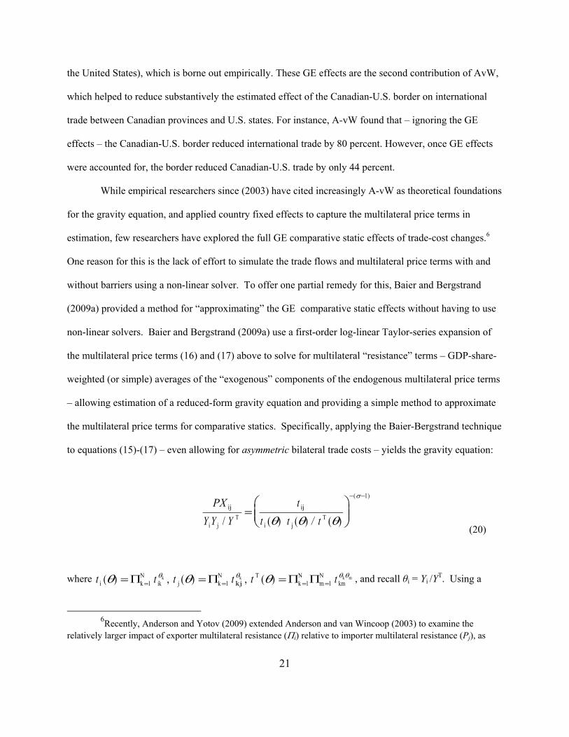
the multilateral price terms for comparative statics. Specifically, applying the Baier-Bergstrand technique

to equations (15)-(17) – even allowing for asymmetric bilateral trade costs – yields the gravity equation:

PX tt t / t

ij

i jT

ij

i jTY Y Y/ ( ) ( ) ( )

( )

=⎛

⎝⎜⎜

⎞

⎠⎟⎟

− −

θ θ θ

σ 1

(20)

where t i k 1N

ik j k 1N

kjT

k 1N

m 1N

kmk k k m( ) , ( ) , ( )θ θ θθ θ θ θ= = == = = =Π Π Π Πt t t t t , and recall θi = Yi /YT. Using a

6Recently, Anderson and Yotov (2009) extended Anderson and van Wincoop (2003) to examine the

relatively larger impact of exporter multilateral resistance (Πi) relative to importer multilateral resistance (Pj), as

22

Monte Carlo analysis, Baier and Bergstrand (2009a) show that virtually identical coefficient estimates

(relative to fixed-effects estimates) can be obtained using their approximation method in a gravity

equation. Moreover, using another Monte Carlo exercise for world trade flows among 88 countries, they

show that 74 percent of GE comparative static effects of forming the European Economic Area are within

5 percent of the comparative statics estimated using the A-vW technique.

B. Unconditional General Equilibrium Approaches

The fundamental difference between unconditional GE approaches and conditional GE ones is the

absence of separability of decisions to produce and consume from decisions to allocate goods across

national borders in unconditional GE models. The conditional GE models described above assume

“endowment economies”; in unconditional GE models, the roles of technology and market structure

become explicit. A consequence of unconditional models is that they can be more closely tied to

prevailing theories of trade, where production functions and market structure are explicit.

The three most prominent unconditional GE approaches in international trade are the Ricardian,

Heckscher-Ohlin (H-O), and Helpman-Krugman (H-K) approaches. The Ricardian approach emphasizes

labor-productivity differentials, the H-O approach relative-factor-endowment differentials, and the H-K

monopolistic competition approach internal economies of scale with tastes for variety as the source of

trade. Interestingly, the unconditional GE approaches toward gravity began with H-K’s monopolistic

competition model, then a H-O approach, and most recently a Ricardian approach.

1. Krugman Approach

The first (unconditional) GE approach surfaced in Krugman (1979). Assume a one-sector

economy with one factor of production, labor (l), and assume CES preferences (like equation (12)) but

where each exporting country has an (endogenously-determined) number of varieties of goods to offer

instead of an arbitrary taste parameter, βi, as assumed in A-vW:

defined in equations (16) and (17), respectively..

23

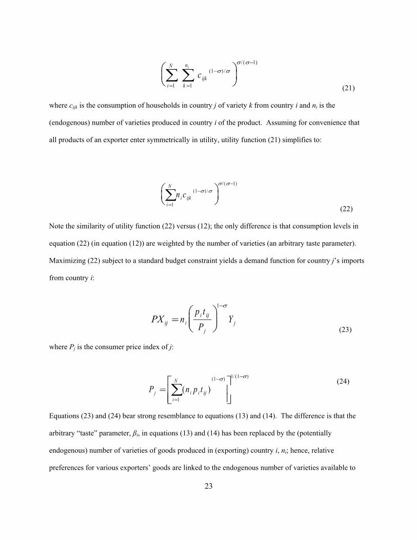
(21)

where cijk is the consumption of households in country j of variety k from country i and ni is the

(endogenous) number of varieties produced in country i of the product. Assuming for convenience that

all products of an exporter enter symmetrically in utility, utility function (21) simplifies to:

(22)

Note the similarity of utility function (22) versus (12); the only difference is that consumption levels in

equation (22) (in equation (12)) are weighted by the number of varieties (an arbitrary taste parameter).

Maximizing (22) subject to a standard budget constraint yields a demand function for country j’s imports

from country i:

(23)

where Pj is the consumer price index of j:

(24)

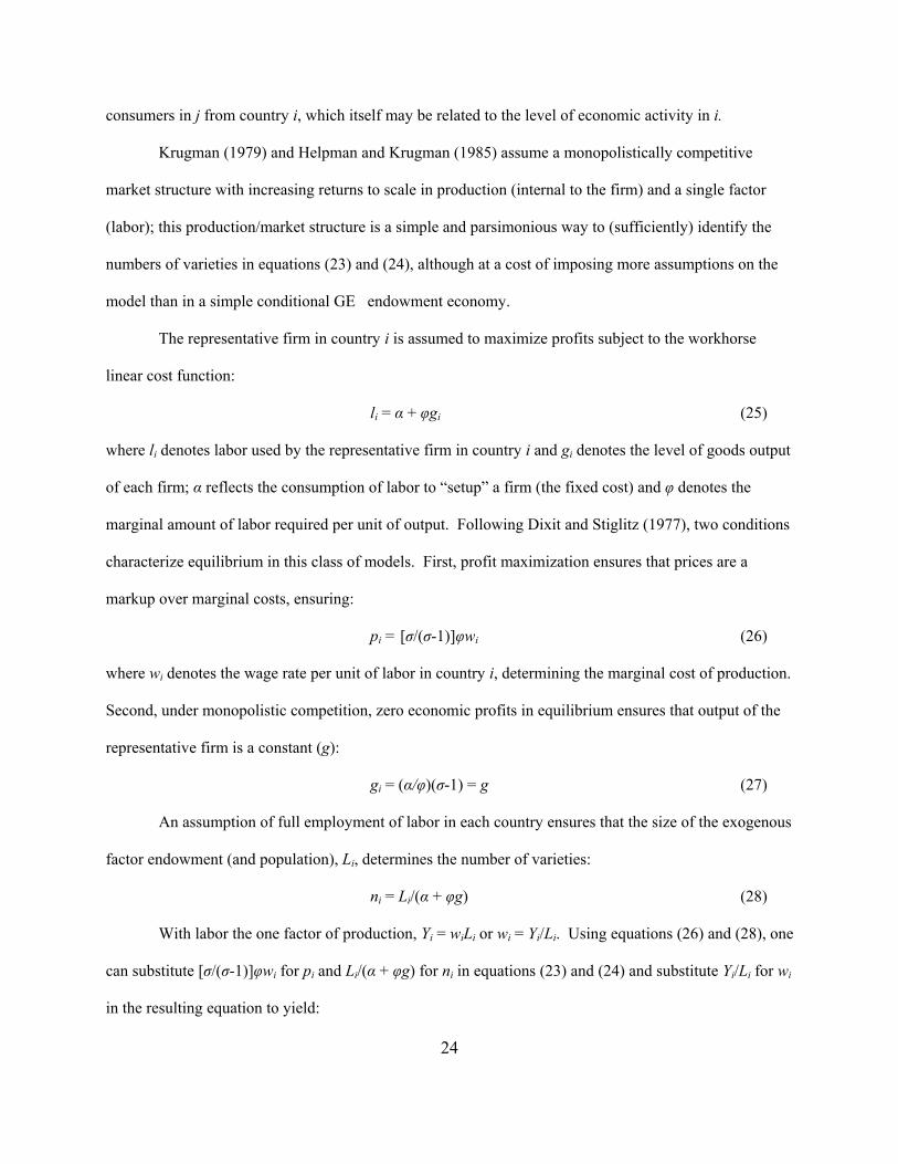
Equations (23) and (24) bear strong resemblance to equations (13) and (14). The difference is that the

arbitrary “taste” parameter, βi, in equations (13) and (14) has been replaced by the (potentially

endogenous) number of varieties of goods produced in (exporting) country i, ni; hence, relative

preferences for various exporters’ goods are linked to the endogenous number of varieties available to

i

N

k

n

ijk

i

c= =

−−

∑ ∑⎛⎝⎜

⎞⎠⎟

1 1

11

( ) // ( )

σ σσ σ

n cii

N

ijk=

−−

∑⎛⎝⎜⎞⎠⎟

1

11

( ) // ( )

σ σσ σ

PX np tP

Yij ii ij

jj=

⎛

⎝⎜⎜

⎞

⎠⎟⎟

−1 σ

P n p tj i i iji

N

=⎡

⎣⎢⎢

⎤

⎦⎥⎥=

− −

∑( )( ) / ( )

1

1 1 1σ σ

24

consumers in j from country i, which itself may be related to the level of economic activity in i.

Krugman (1979) and Helpman and Krugman (1985) assume a monopolistically competitive

market structure with increasing returns to scale in production (internal to the firm) and a single factor

(labor); this production/market structure is a simple and parsimonious way to (sufficiently) identify the

numbers of varieties in equations (23) and (24), although at a cost of imposing more assumptions on the

model than in a simple conditional GE endowment economy.

The representative firm in country i is assumed to maximize profits subject to the workhorse

linear cost function:

li = α + φgi (25)

where li denotes labor used by the representative firm in country i and gi denotes the level of goods output

of each firm; α reflects the consumption of labor to “setup” a firm (the fixed cost) and φ denotes the

marginal amount of labor required per unit of output. Following Dixit and Stiglitz (1977), two conditions

characterize equilibrium in this class of models. First, profit maximization ensures that prices are a

markup over marginal costs, ensuring:

pi = [σ/(σ-1)]φwi (26)

where wi denotes the wage rate per unit of labor in country i, determining the marginal cost of production.

Second, under monopolistic competition, zero economic profits in equilibrium ensures that output of the

representative firm is a constant (g):

gi = (α/φ)(σ-1) = g (27)

An assumption of full employment of labor in each country ensures that the size of the exogenous

factor endowment (and population), Li, determines the number of varieties:

ni = Li/(α + φg) (28)

With labor the one factor of production, Yi = wiLi or wi = Yi/Li. Using equations (26) and (28), one

can substitute [σ/(σ-1)]φwi for pi and Li/(α + φg) for ni in equations (23) and (24) and substitute Yi/Li for wi

in the resulting equation to yield:

25

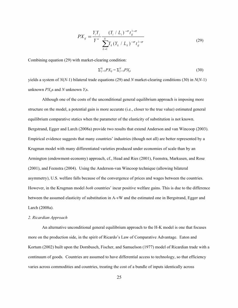
PXY YY

Y L t

Y Y L tij

i jw

i i ij

k k k ijk

N=− −

− −

=∑

( / )

( / )

σ σ

σ σ

1

1

1

(29)

Combining equation (29) with market-clearing condition:

ΣNj =1PXij = ΣN

j =1PXji (30)

yields a system of N(N-1) bilateral trade equations (29) and N market-clearing conditions (30) in N(N-1)

unknown PXijs and N unknown Yis.

Although one of the costs of the unconditional general equilibrium approach is imposing more

structure on the model, a potential gain is more accurate (i.e., closer to the true value) estimated general

equilibrium comparative statics when the parameter of the elasticity of substitution is not known.

Bergstrand, Egger and Larch (2008a) provide two results that extend Anderson and van Wincoop (2003).

Empirical evidence suggests that many countries’ industries (though not all) are better represented by a

Krugman model with many differentiated varieties produced under economies of scale than by an

Armington (endowment-economy) approach, cf., Head and Ries (2001), Feenstra, Markusen, and Rose

(2001), and Feenstra (2004). Using the Anderson-van Wincoop technique (allowing bilateral

asymmetry), U.S. welfare falls because of the convergence of prices and wages between the countries.

However, in the Krugman model both countries’ incur positive welfare gains. This is due to the difference

between the assumed elasticity of substitution in A-vW and the estimated one in Bergstrand, Egger and

Larch (2008a).

2. Ricardian Approach

An alternative unconditional general equilibrium approach to the H-K model is one that focuses

more on the production side, in the spirit of Ricardo’s Law of Comparative Advantage. Eaton and

Kortum (2002) built upon the Dornbusch, Fischer, and Samuelson (1977) model of Ricardian trade with a

continuum of goods. Countries are assumed to have differential access to technology, so that efficiency

varies across commodities and countries, treating the cost of a bundle of inputs identically across

26

X T Yc t

T c tij i j

i ij

k k kjk

N=−

−

=∑

( )

( )

θ

θ

1

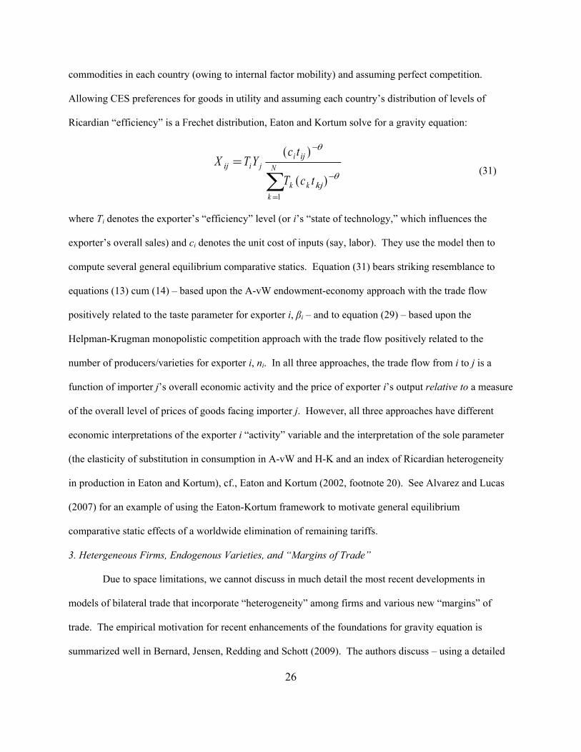
commodities in each country (owing to internal factor mobility) and assuming perfect competition.

Allowing CES preferences for goods in utility and assuming each country’s distribution of levels of

Ricardian “efficiency” is a Frechet distribution, Eaton and Kortum solve for a gravity equation:

(31)

where Ti denotes the exporter’s “efficiency” level (or i’s “state of technology,” which influences the

exporter’s overall sales) and ci denotes the unit cost of inputs (say, labor). They use the model then to

compute several general equilibrium comparative statics. Equation (31) bears striking resemblance to

equations (13) cum (14) – based upon the A-vW endowment-economy approach with the trade flow

positively related to the taste parameter for exporter i, βi – and to equation (29) – based upon the

Helpman-Krugman monopolistic competition approach with the trade flow positively related to the

number of producers/varieties for exporter i, ni. In all three approaches, the trade flow from i to j is a

function of importer j’s overall economic activity and the price of exporter i’s output relative to a measure

of the overall level of prices of goods facing importer j. However, all three approaches have different

economic interpretations of the exporter i “activity” variable and the interpretation of the sole parameter

(the elasticity of substitution in consumption in A-vW and H-K and an index of Ricardian heterogeneity

in production in Eaton and Kortum), cf., Eaton and Kortum (2002, footnote 20). See Alvarez and Lucas

(2007) for an example of using the Eaton-Kortum framework to motivate general equilibrium

comparative static effects of a worldwide elimination of remaining tariffs.

3. Hetergeneous Firms, Endogenous Varieties, and “Margins of Trade”

Due to space limitations, we cannot discuss in much detail the most recent developments in

models of bilateral trade that incorporate “heterogeneity” among firms and various new “margins” of

trade. The empirical motivation for recent enhancements of the foundations for gravity equation is

summarized well in Bernard, Jensen, Redding and Schott (2009). The authors discuss – using a detailed

27

panel data set of firm-level and transaction-level observations for U.S. exporters and importers (including

multinational firms) – the main sources of cross-sectional and time-series variation in U.S. bilateral trade

flows. The data set decomposes, for instance, aggregate bilateral U.S. exports (and imports from) to some

country j into four components: (1) number of U.S. export firms to j, or “extensive margin of firms”; (2)

number of products each firm exports to j, or “extensive margin of products”; the “density” of trade (i.e.,

the share of the number of firm-product observations for which trade is positive); and the “intensive

margin” (i.e., the average value of a firm-product observation). It turns out that – across pairings of

countries in a given year – the vast bulk of variation (about 70 percent) is explained by the extensive

margin of firms. Put simply, larger trade flows are explained predominantly by large countries (in terms

of GDP or populations), which have a large number of firms. Hence, the Helpman-Krugman framework

described above is suitable to explain the vast bulk of variation cross-sectionally in trade flows. Most of

the rest of the cross-sectional variation is explained by the “intensive margin,” that is, variation in average

sales per firm-product. However, in the short-run (say, annually), most of the variation in trade flows is

explained by the intensive margin. Consequently, shocks over time – such as changing trade policies –

may well explain changes in average values of firm-product observations, also consistent with the

frameworks above. Nevertheless, newly-explored margins – such as new products per firm or new

consumers per product-firm-destination – play some role. Their exploration is emphasized in papers such

as Melitz (2003), Chaney (2008), Helpman, Melitz, and Rubinstein (2008), Arkolakis (2008), and Egger,

Larch, Staub, and Winkelmann (2009), among others, which “nest” these features into gravity equations.

C. Empirical Applications

As gravity equations have been estimated using regression techniques for nearly 50 years, the

number of empirical studies is immense. We discuss mostly some recent estimates that have become

useful and whose specifications are based upon rigorous theoretical and econometric foundations.

1. Effects of Economic Integration Agreements

One of the oldest and most prominent uses of the gravity equation has been to estimate the

28

impacts of economic integration agreements (EIAs) – notably, free trade agreements (FTAs), customs

unions, and other forms of preferential trade agreements (PTAs) – on trade. Tinbergen (1962), in the first

gravity equation application to trade, evaluated the effect of (membership in) the BENELUX FTA and the

British Commonwealth on members’ trade. Most studies have examined the trade creation effects, while

a few have also attempted to measure the effects of trade diversion. Some early influential partial EIA

estimates using traditional gravity equations can be found in Linnemann (1966), Aitken (1973), Sapir

(1978), Bergstrand (1985), Brada and Mendez (1985), and Frankel (1997). Partial – or direct – effects

reflect the coefficient estimates on EIA dummies. Such estimates ignore feedback effects on trade flows

from other price changes; we discuss estimation of general equilibrium (GE) effects of EIAs later.

Moreover, Ghosh and Yamarik (2004) use extreme-bounds analysis to find that coefficient estimates of

EIA effects using traditional cross-section gravity equations are quite “fragile.”

In the last decade, researchers have turned more to panel data to estimate the partial effects of

EIAs on trade flows in order to avoid unobservable heterogeneity across country pairs. In a series of

papers, Egger (2000, 2002, 2004) finds overwhelming evidence of fixed-effects specifications over

random-effects specifications (as well as over traditional specifications ignoring unobserved

heterogeneity). However, there are numerous possible fixed-effects specifications. Mátyás (1997)

proposes including an exporter fixed effect, an importer fixed effect, and a time fixed effect (i.e., a set of

time dummies). Egger (2000) finds that a random-effects specification is rejected in favor of such a

fixed-effect specification. Egger and Pfaffermayr (2003) and Cheng and Wall (2005) reject a fixed-effect

specification with exporter effect, importer effect, and time effect in favor of a specification with a

country-pair fixed effect and a time effect; Cheng and Wall (2005) also reject symmetry in the country-

pair effect, which was used in Glick and Rose (2001). Baltagi, Egger, and Pfaffermayr (2003) suggest

estimating models with fixed country-pair and also fixed exporter-year and fixed importer-year effects. In

models à la Eaton and Kortum (2002), Anderson and van Wincoop (2003), or Bergstrand, Egger, and

Larch (2008a) and applications with panel data, fixed exporter-year and fixed importer-year ensure that

29

the coefficients of bilateral trade costs are not biased by omitted general equilibrium effects. In a panel

(endogenous) unobservable multilateral price terms for each country vary over time; consequently, panel

estimation requires exporter-time (it) and importer-time (jt) effects, rather than exporter (i) and importer

(j) effects. Moreover, unobserved heterogeneity in country pairs suggests the inclusion of country-pair

fixed effects (ij), as Cheng and Wall (2005) recommended.

Several recent studies have consequently investigated the effects of EIAs on trade flows

motivated by these theoretical and econometric considerations. Baier and Bergstrand (2007) investigated

the average partial (treatment) effect of numerous EIAs using these country-time and country-pair effects,

finding that the average partial effect of an EIA between a pair of countries on their bilateral trade was

approximately 100 percent after 10-15 years, with little further effect after that (and no permanent

“growth” effects). Baier, Bergstrand, and Vidal (2007) used this technique to find credible effects of

various Latin American EIAs on members’ trade flows. Baldwin and Taglioni (2007) employed exporter-

time, importer-time, and country-pair fixed effects and found smaller EU integration effects and no effect

of Eurozone membership on members’ trade. Baier, Bergstrand, Egger, and McLaughlin (2008) used the

same technique to find plausible effects of various Western European agreements on members’ trade

flows. Gil, Llorca and Martinez-Serrano (2008) used the same methodology to examine the partial trade-

creation and trade-diversion effects of European Community/Union enlargements as well as various other

agreements (including monetary agreements) on members’ trade flows, finding credible estimates.

Two other issues have been raised as important for estimating properly the effects of EIAs on

trade flows. First, the formation of an EIA is not exogenous to trade flows; in fact, most economic factors

that explain trade flows also explain FTA formations, cf., Baier and Bergstrand (2002, 2004). Since

unobservable variables which influence selection into EIAs by pairs of countries’ governments may also

influence trade flows themselves, endogeneity bias arises which may tend to overstate or understate the

true (partial) effect of an EIA in a regression. One method to address this potential endogeneity issue is

the use of instrumental variables (two-stage) estimation, requiring estimation in the first stage of the

30

likelihood of an EIA between a country-pair and then using an instrument for the EIA dummy in the

second stage, cf., Baier and Bergstrand (2002), Carrère (2006), and Egger, Larch, Staub, and Winkelmann

(2009); such a method can be used potentially with cross-section data. A second method to address this

endogeneity bias requires panel data. If decisions to form or enlarge EIAs are slow-moving relative to

trade flows, estimation of EIAs’ effects on trade using exporter-time, importer-time, and country-pair

fixed effects can eliminate potentially the endogeneity bias, cf., Baier and Bergstrand (2007), Baldwin

and Taglioni (2007), and the other studies cited in the previous paragraph.

Second, as noted as early as Linnemann (1966), half of the world’s bilateral trade flows are zero.

Given recent developments in the theory of international trade to examine firm “heterogeneity” (Melitz,

2003) and the existence of national data sets of countries’ firms/plants international trade flows, theories

have surfaced to explain which countries select into international trade and consequently why half of the

world’s bilateral trade flows are zero. Helpman, Melitz, and Rubinstein (2008) use the Melitz (2003)

model to setup a two-stage system for estimating gravity models. The first stage is predicting which

country pairs trade, given the existence of fixed costs to trade in the Melitz model and selection issues.

Conditioned upon a positive trade flow, the second stage provides a Helpman-Krugman-based model of

economic determinants of trade flows. The zeros issue was also addressed in Santos Silva and Tenreyro

(2006) using a Poisson quasi-maximum-likelihood estimator in their effort to eliminate bias arising from

hetereoskedasticity in the error terms in typical gravity equations; Westerlund and Wilhelmsson (2009)

also use a Poisson estimator to address the zeros issue in gravity models and Felbermayr and Kohler

(2004) a Tobit estimator. Baldwin and Harrigan (2007) address the zeros issue in terms of examining

divergent predictions of various trade models for explaining observed trade prices and offer a modified

Melitz model of heterogeneous firm behavior. Both zero trade flows and bias arising from endogeneity of

EIA dummies were addressed simultaneously in Egger, Larch, Staub and Winkelmann (2009). They find

that ignoring endogeneity bias of EIAs is relatively more important than ignoring selection bias into

trading (the zero-trade-flow issue). Accounting for endogeneity of EIAs raises the estimated long-run,

31

general equilibrium impact of an EIA on members’ trade by about 40 percentage points, doubling the GE

effect of assuming exogenous EIAs. Accounting for “selection” into trade flows raises the estimated

impact of an EIA by only 10 percentage points.

2. Trade and Growth

The gravity equation has found an important use in helping to understand the effects of trade on

economic growth. There is a large literature examining the effects of trade and “openness” on countries’

levels of per capita income – alongside the influences of institutions and geography. However, unlike

geography, trade and per capita incomes are determined simultaneously, so coefficient estimates of

regressions of per capita incomes on measures of trade (alongside other determinants) are potentially

biased by endogeneity issues. One important paper addressing this issue is Frankel and Romer (1999).

Since trade is endogenous, they needed an instrument for trade that is exogenous to per capita incomes.

Since gravity equations using populations (instead of GDPs), distance, and other exogenous variables can

predict well bilateral trade flows, the predicted values of these flows could generate an (exogenous)

instrumental variable for trade openness. Using this technique, they demonstrated that trade has an

economically and statistically significant effect on per capita income, raising per capita GDP by almost

one percent for every one percent higher trade relative to GDP. Alcala and Ciccone (2004) used the

Frankel-Romer procedure along with instruments to account for the endogeneity of the “institutions”

variable to show that – accounting for institutions properly – trade openness retained its economically and

statistically significant effect on per capita income.

Badinger (2008) extended this type of analysis further to show the positive impacts of EIAs on

productivity levels across countries (which then raise per capita incomes). Following Baier and

Bergstrand (2004), Badinger predicted bilateral trade flows to construct an instrument for trade openness,

accounting for the endogeneity between EIAs and trade flows discussed earlier. Using instruments for

EIAs to help predict trade flows, Badinger (2008) found that trade openness – alongside institutions and

geography – has an economically and statistically significant effect on productivity levels (and by

32

extension per capita incomes).

3. Infrastructure, Currency Unions, Political and Institutional Factors, and Immigrant Stocks

As noted earlier, the gravity equation has been used extensively to estimate the impact of

numerous other factors on the volume of trade; another entire survey would be needed to discuss

comprehensively all of these efforts. Hence, the remainder of this section addresses each of four other

important areas of application of the gravity equation briefly.

Traditionally, the gravity equation has included variables associated with marginal trade costs,

such as distance representing maritime and air transport costs. However, as recent developments in trade

theory to account for firm heterogeneity (cf., Melitz, 2003, Yeaple, 2005) suggest, fixed costs play a role

in determining both selection into international trade as well as its volume. Infrastructure for trade is a

likely important factor in influencing both the existence as well as the level of trade. Recently, several

studies have examined the impact of trade infrastructure on bilateral trade flows using gravity equations.

One of the earliest papers addressing the importance of infrastructure for trade was Limão and Venables

(2001). For instance, using a gravity framework, Limão and Venables (2001) found that reducing the

quality and degree of infrastructure from the median to the 75th percentile increased trade costs by 12

percent and reduced the volume of trade by 28 percent. Guided by an Eaton-Kortum-based general

equilibrium model, Donaldson (2009) finds that the railroad system in India decreased trade costs,

increased interregional and international trade, and improved productivity significantly. Other papers

finding significant effects of infrastructure on trade flows include Francois and Manchin (2007),

Grigoriou (2007), Shepherd and Wilson (2007), and De (2008).

Beginning with Abrams (1980) and Thursby and Thursby (1987), the gravity equation has been

used for decades to examine the effects of exchange rate variability and – more recently – of currency

unions on international trade flows. Rose (2000) started a cottage-industry in the literature on monetary

arrangements, finding using a gravity equation that membership in a common currency union increased

bilateral trade (the partial effect) of 235 percent. The large size of this effect spurred considerable debate

33

and a large number of critiques. Baldwin (2005) summarized several of the arguments that have been

offered to explain this large estimated effect, which was associated with very small, poor, and open

economies. Among the concerns were potential biases arising from pro-trade effects that were omitted

and likely correlated with the currency union dummy, a concern about reverse causality (big trade flows

causing formation of currency unions), and possible model mis-specification.

The gravity equation has been used extensively in political science circles as well. For instance,

early applications of the traditional gravity equation to examine the influences of conflict, political

cooperation, detente, etc. on trade flows include Summary (1989), Pollins (1989), van Bergijk and

Oldersma (1990), Gowa and Mansfield (1993), and Mansfield and Bronson (1997). Polachek (1980) was

one of the first to examine formally the relationship between conflict and trade, and Polachek has worked

extensively on the simultaneity between conflict and trade, cf., Polachek and Seiglie (2006). Reuveny

and Kang (2003) extended analysis of simultaneous determination of conflicts and trade using gravity

equations. Mansfield, Milner and Rosendorff (2000) examine the roles of democratic institution and

governments’ choice of trade policies for influencing trade flows, and cite many related articles.

Anderson and Marcouiller (2002) explored the role of government institutions regarding “insecurity” and

trade flows in a gravity framework. More recently, the gravity equation has been used with general-

equilibrium theoretical foundations to explore violence, war, and trade flows, cf., Blomberg and Hess

(2006), Martin, Mayer and Thoenig (2008), and Glick and Taylor (2009).

The gravity equation has also been used to link trade and migration flows. Gould (1994)

extended the theoretical foundations for the gravity equation in Bergstrand (1985) to examine the role of

immigrant stocks in home and host countries for influencing trade flows, which is motivated by the role

that immigrant stocks play in providing informational advantages. Supporting evidence for this is found

in Head and Ries (1998), Dunlevy and Hutchinson (1999), Rauch (1999, 2001), Rauch and Trindade

(2002), and Girma and Yu (2002).

4. General-Equilibrium-Motivated Gravity Models of Trade, Investment, and Migration

34

Although the gravity equation has been used more extensively to study patterns of international

trade, it has also been used prominently to study foreign direct investment (FDI) flows as well as

migration flows. As mentioned earlier, the gravity equation was first used to study migration patterns,

long before studying trade and FDI flows. However, space constraints prevent much discussion here of

the study of migration flows. But the prominence of multinational firms in the world economy – which

by nature have foreign investments, affiliates, and operations – suggests some discussion of the

complementarity and substitutability of trade and FDI flows. Moreover, the gravity equation has gained

increasing popularity in the study of FDI flows.

A. General Equilibrium Foundations for the Gravity Equation of Trade, FDI, and Skilled Migration

Blonigen (2005) noted two important facts regarding the use of the gravity equation for modeling

bilateral FDI flows. First, the empirical specification most frequently used in the study of economic

determinants of FDI flows is the gravity equation. Second, theoretical justification for using the gravity

equation has been usually by analogy to trade flows. Unlike the extensive general equilibrium theoretical

foundations for gravity equations of trade flows, there has been no general equilibrium theoretical

foundation provided for FDI flows until very recently.

At the same time that gravity equations have flourished in the empirical analysis of FDI flows

over the past twenty years, general equilibrium theoretical foundations for the existence of multinational

firms and foreign affiliate operations surfaced quite separately. However, only recently have the general

equilibrium foundations broadened to provide a theoretical foundation for FDI flows and trade flows

simultaneously. Since we will discuss empirical applications later, we focus in this section on a general

equilibrium theoretical foundation for gravity equations of FDI and trade.

The starting point for general equilibrium analysis of national and multinational enterprises (NEs

and MNEs, respectively) is summarized in an earlier chapter in this volume by Markusen, the details of

which are comprehensively discussed in Markusen (2002). Much of Markusen (2002) is based upon

earlier papers, cf., Markusen (1984), Markusen and Venables (1998), Markusen and Venables (2000), and

35

Carr, Markusen and Maskus (2001). Consequently, we discuss only some recent advances that build upon

these 2x2x2 models of MNEs that provide theoretical foundations for estimating gravity equations of FDI

and foreign affiliate sales (FAS).

Only a few recent papers have attempted to provide theoretical foundations for the gravity

equation of FDI and FAS flows. Motivated by the puzzle in the Markusen-Venables (M-V) 2x2x2 GE

model of NEs and MNEs that two countries with identical relative factor endowments maximize their

bilateral FAS when their absolute factor endowments (and hence GDPs) are identical but have zero (intra-

industry) bilateral trade, Bergstrand and Egger (2004, 2007) introduced a third factor (internationally-

mobile physical capital) and a third country (Rest-of-World, or ROW) to resolve this puzzle and motivate a

rationale for estimating gravity equations of FDI and trade simultaneously. First, the reason for the M-V

puzzle can be attributed to only two factors in the M-V model. With headquarter and plant setups

requiring skilled labor, when two countries are identical in absolute and relative factor endowments (for

given bilateral trade and investment costs), both countries tend to be more efficiently served by horizontal

MNEs with headquarters in their home countries but plants in home and foreign countries, rather than ship

large volumes via trade.7 Since MNEs require more skilled labor than national firms for setups, the higher

relative price of skilled (-to-unskilled) labor when the countries are equally-sized “crowds-out” entirely

national exporting firms, yielding large FDI but zero intra-industry trade in equally-sized economies. The

addition of (imperfectly-internationally-mobile) physical capital to the 2x2x2 M-V model – along with the

assumption that plant setups require physical capital and headquarter setups require human capital – easily

resolves this puzzle. As two countries become identical in economic size (for given trade and investment

costs), the higher relative demand for MNEs over NEs increases the relative price of physical-to-human

capital due to the shift from single-plant NEs to multi-plant MNEs. The rise in the relative price of

7If one country is much larger than the other, the larger country can more efficiently serve the foreign

market by exporting to it.

36

physical-to-human capital dampens the increase in MNEs and the decrease in NEs, allowing NEs to co-

exist with MNEs even if the two countries are identical in every aspect. However, in the Bergstrand-

Egger model, intra-industry trade is not maximized when the two countries are identical, when only two

countries are allowed. However, further extension of the model to three countries leads to an even

stronger dampening of the shift from single-plant NEs to multi-plant MNEs, such that the relationships

between bilateral FDI (and FAS) and trade with economic size and similarity can be approximated by the

“gravity equation.” A further extension of the Bergstrand-Egger model to allow imperfectly-

internationally-immobile skilled labor yields simultaneous theoretical gravity equations for bilateral

international trade, FDI, and skilled migration flows, cf., Bergstrand, Egger, and Larch (2008b).

Only a few other papers have attempted to motivate gravity equations for FAS. Grazalian and

Furtan (2005), Kleinert and Toubal (2005), and Lai and Zhu (2006) assume models with exogenously

heterogeneous productivities to generate co-existence of MNEs and NEs, in the spirit of the model in

Helpman, Melitz, and Yeaple (2004), but do not address simultaneously FDI and trade. Shim (2005)

extends the Anderson and van Wincoop (2003) conditional GE model of trade to include FAS to further

explain the McCallum “border puzzle,” but must assume exogenously the unique equilibrium in Markusen

and Venables (2000) to generate the coexistence of NEs and MNEs (attributable to the two-factor

limitation in the M-V model). Head and Ries (2008) extend the theoretical foundations for a gravity

equation of FDI in order to explore the motive of “corporate control” for determining FDI flows.

B. Empirical Applications

The most common tool to analyze observed bilateral FDI flows is the gravity equation. As for

trade flows, the gravity model has been applied to analyze empirically the effects on FDI flows of various

economic and political considerations. A complete review of such studies is beyond the scope of this

chapter; however, some more recent applications are indicative of its usefulness.

As for trade flows, gravity equations have been used to analyze the effects of natural impediments

37

to FDI. One of the earliest applications of the gravity equation to FDI flows is Eaton and Tamura (1994).

This study was one of the first to identify that both trade and FDI flows have positive relationships with

market size and similarity using similar specifications. While Eaton and Tamura (1994) used regional

dummies instead of bilateral distance, most studies have found that distance has a significant negative

impact on FDI flows. Since most FDI tends to be horizontal in nature, and a substitute for trade, this

negative impact implies that distance may not be representing transport costs of goods, as the “proximity-

concentration” ratio hypothesis would suggest, cf., Brainard (1993) and Markusen (2002). Schatz and

Venables (2000) confirmed that “Distance and market size are extremely important in determining where

firms establish their foreign affiliates.” In an extension of the proximity-concentration-ratio hypothesis,

Irac (2004) suggests that distance may have a negative effect if the fixed cost of a new plant outweighs

transport costs; she shows that cultural differences are a large impediment for FDI. While most gravity

equations include distance and GDPs, recent work has looked at “spatial” lag models, cf., Blonigen,

Davies, Waddell and Naughton (2007). For instance, regions/countries with large GDPs and surrounded

by large markets tend to have more FDI, suggesting export-platform FDI, which has been uncovered using

spatial-lag models. Also, natural costs to FDI are not limited to distance. For instance, Stein and Duade

(2007) use a gravity equation to estimate the negative effects of time on FDI and trade. They find that time

zones have a strong effect on both, but is relatively stronger on FDI than trade.

As with trade, the gravity equation has been used to examine the impacts of (man-made)

investment policies on FDI flows. Blonigen and Davies (2004) estimate that bilateral tax treaties have

increased FDI flows by 2-8 percent for each year of the treaty. They find moreover that, while treaties have

an immediate impact on FDI, there is a substantial lag before treaty adoptions positively affect FDI stocks

and foreign affiliate sales. Egger and Pfaffermayr (2004) also find evidence of bilateral investment treaties

on FDI. Mutti and Grubert (2004) use a gravity equation to examine tax rates explicitly on types of MNE

FDI decisions. Smith (2001) used a gravity equation to examine whether foreign patent rights affect U.S.

38

exports, affiliate sales, and licenses. She found that strong foreign patent rights increase U.S. affiliate sales

and licenses, particularly across countries with strong imitative abilities. Globerman and Shapiro (2002)

and Bénassy-Quéré, Coupet and Mayer (2007) find that the quality of governance institutions is important

for FDI flows.

Some researchers have even examined the impact of trade policies on FDI flows (and then

subsequently, investment policies on trade flows) using gravity equations. For instance, Baltagi, Egger

and Pfaffermayr (2008) use a spatial-lag model to isolate the effects of regional trade agreements on FDI

flows. Trade liberalization of a set of parent countries with some host markets leads to a relocation of FDI

from other hosts into the liberalizing ones. Amiti and Wakelin (2003) estimate the cross-price elasticity of

exports with respect to investment liberalizations. When countries’ differences in relative factor

endowments are large and levels of trade costs are small, investment liberalization stimulates exports, but

when the reverse conditions hold investment liberalization reduces exports. Two other recent studies

examining the effects of trade agreements on FDI are Levy-Yeyati, Stein, and Daude (2002a, 2002b).

Finally, Norbäck, Urban, and Westerberg (2007) find evidence that accession to the World Trade

Organization significantly increases the export intensity of foreign affiliates of MNEs.

5. Conclusions

The gravity equation has been used for over fifty years in examining empirically the economic,

political, and cultural determinants of bilateral trade, FDI, and migration flows – that is, of globalization.

Theoretical foundations have been developed over the last thirty years that provide a rigorous, logical,

economic rationale for its econometric use, although such foundations are not yet complete. However, the

advancement of our theoretical understanding of the gravity equation – specifically, the roles of frictions,

economic size and similarity, and relative factor endowments – have certainly enhanced the equation’s

usefulness as a tool for policymakers in determining the effects of various policies on the flows that

comprise globalization. Nevertheless, much theoretical and empirical analysis is still needed to further

39

help our understanding of the determinants of trade, FDI, and migration flows, which will consequently

help policy-makers institute welfare-improving policies in a global economy.

References

Abrams, Richard K., 1980. “International Trade Flows under Flexible Exchange Rates.” Economic Review, Federal Reserve Bank of Kansas City, March, 3-10.

Aitken, Norman D., 1973. “The Effect of EEC and EFTA on European Trade: A Temporal Cross-Section

Analysis,” American Economic Review, volume 63, number 5, December, 881-892. Alcala, Francisco, and Antonio Ciccone, 2004. “Trade and Productivity,” Quarterly Journal of

Economics, volume 119, number 2, May, 613-646. Alvarez, Fernando, and Robert E. Lucas, Jr., 2007. “General Equilibrium Analysis of the Eaton-Kortum

Model of International Trade,” Journal of Monetary Economics, volume 54, 1726-1768. Amiti, Mary, and Katherine Wakelin, 2003. “Investment Liberalization and International Trade,” Journal

of International Economics, volume 61, number 1, October, 101-126. Anderson, James E., 1979. “A Theoretical Foundation for the Gravity Equation,” American Economic

Review, volume 69, number 1, March, 106-116. Anderson, James E., and Douglas Marcouiller, 2002. “Insecurity and the Pattern of Trade: An Empirical

Investigation,” Review of Economics and Statistics, volume 84, number 2, May, 342-352. Anderson, James E., and Eric van Wincoop, 2003. “Gravity with Gravitas,” American Economic Review,

volume 93, number 1, March, 170-192. Anderson, James E., and Eric van Wincoop, 2004. “Trade Costs,” Journal of Economic Literature,

volume 42, September, 691-751. Anderson, James E., and Yoto V. Yotov, 2009. “The Changing Incidence of Geography,” working paper,

Boston College. Arkolakis, Costas, 2008. “Market Penetration and the New Consumers Margin in International Trade,”

working paper, Yale University. Badinger, Harald, 2008. “Trade Policy and Productivity,” European Economic Review, volume 52, July,

867-891. Baier, Scott L., and Jeffrey H. Bergstrand, 2001. “The Growth of World Trade: Tariffs, Transport Costs,

and Income Similarity,” volume 53, number 1, February, 1-27. Baier, Scott L., and Jeffrey H. Bergstrand, 2002. “On the Endogeneity of International Trade Flows and

Free Trade Agreements,” working paper, University of Notre Dame.

40

Baier, Scott L., and Jeffrey H. Bergstrand, 2004. “Economic Determinants of Free Trade Agreements”

Journal of International Economics, volume 64, number 1, October, 29-63. Baier, Scott L., and Jeffrey H. Bergstrand, 2007. “Do Free Trade Agreements Actually Increase Members’

International Trade?” Journal of International Economics, volume 71, number 1, March, 72-95. Baier, Scott L., Jeffrey H. Bergstrand, and Erika Vidal, 2007. “Free Trade Agreements In the Americas:

Are the Trade Effects Larger than anticipated?,” The World Economy, volume 30, number 9, September, 1347-1377.

Baier, Scott L, Jeffrey H. Bergstrand, Peter Egger, and Patrick McLaughlin, 2008. “Do Economic

Integration Agreements Actually Work? Issues in Understanding the Causes and Consequences of the Growth of Regionalism,” The World Economy, volume 31, number 4, April, 461-497.

Baier, Scott L., and Jeffrey H. Bergstrand, 2009a. “Bonus Vetus OLS: A Simple Method for

Approximating International Trade-Cost Effects using the Gravity Equation,” Journal of International Economics, volume 77, number 1, February, 77-85.

Baier, Scott L., and Jeffrey H. Bergstrand, 2009b. “Estimating the Effects of Free Trade Agreements on

International Trade Flows using Matching Econometrics,” Journal of International Economics, volume 77, number 1, February, 63-76.

Baldwin, Richard E., 2005. “The Euro’s Trade Effect,” paper prepared for a European Central Bank

workshop. Baldwin, Richard E., and James Harrigan, 2007. “Zeros, Quality and Space: Trade Theory and Trade

Evidence,” National Bureau of Economic Research Working Paper 13214, July. Baldwin, Richard E., and Daria Taglioni, 2007. “Trade Effects of the Euro: A Comparison of Estimators,”

Journal of Economic Integration, volume 22, number4, December, 780 Baltagi, Badi H., Peter Egger, and Michael Pfaffermayr, 2003. “A Generalized Design for Bilateral Trade

Flow Models,” Economics Letters, volume 80, 391-397. Baltagi, Badi H., Peter Egger, and Michael Pfaffermayr, 2008. “Estimating Regional Trade Agreement

Effects on FDI in an Interdependent World,” Journal of Econometrics, volume 145, 194-208. Belderbos, Rene, 1997. “Antidumping and Tariff Jumping Japanese Firms’ DFI in the European Union

and United States,” Weltwirtschaftliches Archiv, volume 133, 419-457. Bénassy-Quéré, Agnès, Maylis Coupet, and Thierry Mayer, 2007. “Institutional Determinants of Foreign

Direct Investment,” The World Economy, volume 30, number 5, May, 764-782. Bergstrand, Jeffrey H., 1981. The Gravity Equation in International Trade. Ph.D. dissertation, Department

of Economics, University of Wisconsin at Madison.

41

Bergstrand, Jeffrey H., 1985. “The Gravity Equation in International Trade: some Microeconomic Foundations and Empirical Evidence,” Review of Economics and Statistics, volume 67, number 3, August, 474-481.

Bergstrand, Jeffrey H., and Peter Egger, 2004. “A Theoretical and Empirical Model of International Trade

and Foreign Direct Investment with Outsourcing: Part 1, Developed Countries,” working paper, University of Notre Dame.

Bergstrand, Jeffrey H., and Peter Egger, 2007. “A Knowledge-and-Physical-Capital Model of International

Trade Flows, Foreign Direct Investment, and Multinational Enterprises,” Journal of International Economics, volume 73, number 2, 278-308.

Bergstrand, Jeffrey H., and Peter Egger, 2009. “A General Equilibrium Theory for Estimating Gravity

Equations of Bilateral FDI, Final Goods Trade, and Intermediate Goods Trade,” in S. Brakman and P. van Bergeijk (eds.), The Gravity Model in International Trade: Advances and Applications, Cambridge University Press, Cambridge, UK, forthcoming.

Bergstrand Jeffrey H., Peter Egger, and Mario Larch, 2008a. “Gravity Redux: Structural Estimation of

Gravity Equations, Elasticities of Substitution, and Economic Welfare under Asymmetric Bilateral Trade Costs,” University of Notre Dame working paper.

Bergstrand, Jeffrey H., Peter Egger, and Mario Larch, 2008b. “The New Expats: Economic Determinants

of Bilateral Expatriate, FDI, and International Trade Flows,” University of Notre Dame working paper.

Bernard, Andrew B., J. Bradford Jensen, Stephen J. Redding, and Peter K. Schott (2009). “The Margins of

U.S. Trade (Long Version),” working paper CES 09-18, U.S. Census Bureau. Blomberg, S, and Gregory D. Hess, 2006. “How Much Does Violence Tax Trade?” Review of Economics

and Statistics, volume 88, number 4, 599-612. Blonigen, Bruce A., 2002. “Tariff-Jumping Antidumping Duties,” Journal of International Economics,

volume 57, number 1, 31-50. Blonigen, Bruce A., and Ronald Davies, 2004. “The Effects of Bilateral Tax Treaties on U.S. FDI

Activity,” International Tax and Public Finance, volume 11, 601-622. Blonigen, Bruce A., Ronald Davies, Glen R. Waddell, and Helen Naughton, 2007. “FDI in Space: Spatial

Autoregressive Relationships in Foreign Direct Investment,” European Economic Review, volume 51, number 5, July, 1303-1325.

Borjas, George J, 1994. “The Economics of Immigration,” Journal of Economic Literature, volume 32,

number 4, December, 1667-1717. Borjas, George J., 1999. The Economic Analysis of Immigration,” in O.C. Ashenfelter and David Card

(eds.), Handbook of Labor Economics, Elsevier Science, Amsterdam, The Netherlands.

42

Brada, Josef C., and Jose A. Mendez, 1985. “Economic Integration among Developed, Developing, and Centrally Planned Economies: A Comparative Analysis,” Review of Economics and Statistics, volume 67, number 4, November, 549-556.

Brainard, Lael S., 1997. “An Empirical Assessment of the Proximity-Concentration HypothesisTrade-Off

between Multinational Sales and Trade,” American Economic Review, volume 87, number 4, September, 520-544.

Carey, H.C., 1865. Principles of Social Science. Philadelphia: J.B. Lippincott and Company. Carr, David, James R., Markusen, and Keith E. Maskus, 2001. “Estimating the Knowledge-Capital Model

of the Multinational Enterprise,” American Economic Review, volume 91, number 3, June, 693-708.

Carrère, Céline, 2006. “Revisiting the Effects of Regional Trade Agreements on Trade Flows with Proper

Specification of the Gravity Model,” European Economic Review, volume 50, 223-247. Chaney, Thomas, 2008. “Distorted Gravity: The Intensive and Extensive Margins of International Trade,”

American Economic Review, volume 98, number 4, September, 1707-1721. Cheng, I.-Hui, and Howard J. Wall, 2005. “Controlling for Heterogeneity in Gravity Models of Trade,”

Federal Reserve Bank of St. Louis Review, January/February, 49-63. De, Prahir, 2008, “Trade Costs and Infrastructure: Analysis of the Effects of Trade Impediments in Asia,”

Integration and Trade, number 28, January-June, 241-265. Desai, Mihir A., Fritz C. Foley, and James R. Hines, Jr., 2004, “Foreign Direct Investment in a World of

Multiple Taxes,” Journal of Public Economics, volume 88, number 12, 2727-2744. Disdier, Anne-Celia, and Keith Head, 2008. “The Puzzling Persistence of the Distance Effect on Bilateral

Trade,” Review of Economics and Statistics, volume 90, number 1, February, 37-48. Dixit, Avinash, and Joseph E., 1977. “Monopolistic Competition and Optimum Product Diversity,”

American Economic Review, volume 67, number 3, June, 297-308. Donaldson, David, 2009, “Railroads of the Raj: Estimating the Impact of Transportation Infrastructure,”

London School of Economics working paper, June. Dornbusch, Rudiger, Stanley Fischer, and Paul A. Samuelson, 1977. “Comparative Advantage, Trade, and

Payments in a Ricardian Model with a Continuum of Goods,” American Economic Review, volume 67, 823-839.

Dunlevy, James A., and William K. Hutchinson, 1999. “The Impact of Immigration on American Import

Trade in the Late Nineteenth and Early Twentieth Centuries,” The Journal of Economic History, volume 59, 1043-1062.

Eaton, Jonathan, and Akiko Tamura, 1994. “Bilateralism and Regionalism in Japanese and U.S. Trade and

43

Direct Foreign Investment Patterns,” Journal of the Japanese and International Economies, volume 8, number 4, December, 478-510.

Eaton, Jonathan, and Samuel Kortum, 2002. “Technology, Geography, and Trade,” Econometrica, volume

70, 1741-1780. Egger, Peter, 2000. “A Note on the Proper Econometric Specification of the Gravity Equation,” Economics

Letters, volume 66, 25-31. Egger, Peter, 2002. “An Econometric View on the Estimation of Gravity Models and the Calculation of

Trade Potentials,” The World Economy, volume 25, 297-312. Egger, Peter, 2004. “On the Problem of Endogenous Unobserved Effects in the Estimation of Gravity

Models,” Journal of Economic Integration, volume 19, 182-191. Egger, Peter, and Michael Pfaffermayr, 2003. “The Proper Panel Econometric Specification of the Gravity

Equation: A Three-Way Model with Bilateral Interaction Effects,” Empirical Economics , volume 28, 571-580.

Egger, Peter, and Michael Pfaffermayr, 2004. “The Impact of Bilateral Investment Treaties on Foreign

Direct Investment,” Journal of Comparative Economics, volume 32, 788-804. Egger, Peter, Mario Larch, Kevin E. Staub, and Rainer Winkelmann, 2009. “The Trade Effects of

Endogenous Preferential Trade Agreements,” working paper, University of Zurich. Feenstra, Robert C., 2004. Advanced International Trade. Princeton, New Jersey, USA: Princeton

University Press. Feenstra, Robert C., James R. Markusen, and Andrew K. Rose, 2001. “Using the Gravity Equation to

Differentiate among Alternative Theories of Trade,” Canadian Journal of Economics, volume 34, number 2, May, 430-447.

Felbermayr, Gabriel, and Wilhelm Kohler, 2006. “Exploring the Intensive and Extensive Margins of

World Trade,” Review of World Economics, volume 142, 642-674. Francois, Joseph, and Miriam Manchin, 2007, “Institutions, Infrastructure, and Trade,” World Bank Policy

Research Working Paper 4152, March. Frankel, Jeffrey H., 1997. Regional Trading Blocs in the World Economic System. Washington, DC, USA:

Institute for International Economics. Frankel, Jeffrey, and David Romer, “Does Trade Cause Growth?” American Economic Review, volume 89,

number 3, June, 379-399. Frankel, Jeffrey, and Andrew K. Rose, 2002. “An Estimate of the Effect of Common Currencies on Trade

and Income,” Quarterly Journal of Economics, volume 117, number 2, May, 437-466.

44

Freeman, Richard B., 2006. “People Flows in Globalization,” Journal of Economic Perspectives, volume 20, number 2, Spring, 145-170.

Ghosh, Sucharita, and Steven Yamarik, 2004. “Are Regional Trading Arrangements Trade Creating? An

Application of Extreme Bounds Analysis,” Journal of International Economics, volume 63, number 2, July, 369-395.

Gil, Salvador, Rafael Llorca, and J. Antonio Martinez-Serrano, 2008. “Assessing the Enlargement and

Deepening of the European Union,” The World Economy, volume 31, number 9, September, 1253-1272.

Girma, Sourafel, and Zhihao Yu, 2002. “The Link between Immigration and Trade: Evidence from the

United Kingdom,” Weltwirtschaftliches Archiv, volume 138, number 1, 115-130. Glick, Reuven, and Andrew K. Rose, 2001. “Does a Currency Union Affect Trade? The Time-Series

Evidence,” National Bureau of Economic Research Working Paper No. 8396, July. Glick, Reuven, and Alan M. Taylor, 2009. “Collateral Damage: Trade Disruption and the Economic

Impact of War,” Review of Economics and Statistics, forthcoming. Globerman, Steven, and Daniel Shapiro, 2002. “Global Foreign Direct Investment Flows: The Role of

Governance Infrastructure,” World Development, volume 30, number 11, 1899-1919. Gould, David, 1994. “Immigrant Links to the Home Country: Empirical Implications for U.S. Bilateral

Trade Flows,” Review of Economics and Statistics, volume 76, number 2, May, 302-316. Gowa, Joanne, and Edward D. Mansfield, “Power Politics and International Trade,” American Political

Science Review, volume 87, number 2, June, 408-420. Grazalian, Pascal L., and W. Hartley Furtan, 2005. “The Border Effects: Recognizing the Role of FDI,”

working paper, University of Saskatchewan. Grigoriou, Christopher, 2007, “Landlockedness, Infrastructure, and Trade: new Estimates for central Asian

Countries,” World Bank Policy Research Working Paper 4335, August. Grogger, Jeffrey, and Gordon H. Hanson, 2008. “Income Maximization and the Selection and sorting of

International Migrants,” National Bureau of Economic Research Working Paper No. 13821. Hanson, Gordon H., 2006. “Illegal Migration from Mexico to the United States,” Journal of Economic

Literature, volume 44, number 4, December, 869-924. Hatton, Timothy J., and Jeffrey G. Williamson, 2002. “What Fundamentals Drive World Migration?”

National Bureau of Economic Research Working Paper No. 9159. Hatton, Timothy J., and Jeffrey G. Williamson, 2005. Global Migration and the World Economy, MIT

Press, Cambridge, Massachusetts, USA.

45

Head, Keith, and John Ries, 1998. “Immigration and Trade Creation: Econometric Evidence from Canada,” Canadian Journal of Economics, volume 31, number 1, February, 47-62.

Head, Keith, and John Ries, 2001. “Increasing Returns versus National Product Differentiation as an

Explanation for the Patter of U.S.-Canada Trade,” American Economic Review, volume 91, number 4, September, 858-876.

Head, Keith, and John Ries, 2008. “FDI as an Outcome of the Market for Corporate Control: Theory and

Evidence,” Journal of International Economics, volume 74, number 1, January, 2-20. Helpman, Elhanan, and Paul Krugman, 1985. Market Structure and Foreign Trade. Cambridge,

Massachusetts, USA: MIT Press. Helpman, Elhanan, Marc J. Melitz, and Yona Rubinstein, 2008. “Estimating Trade Flows: Trading

Partners and Trading Volumes,” Quarterly Journal of Economics, volume 123, number 2, May. Helpman, Elhanan, Marc J. Melitz, and Stephen R. Yeaple, 2004. “Export versus FDI with Heterogeneous

Firms,” American Economic Review, volume 94, number 1, March, 300-316. Hummels, David, 1999. “Toward a Geography of Trade Costs,” working paper, University of Chicago. Hummels, David, 2001. “Time as a Barrier to Trade,” working paper, Purdue University. Hummels, David, 2007. “Transportation Costs and International Trade in the Second Era of

Globalization,” Journal of Economic Perspectives, volume 21, number 3, 131-154. Irac, Delphine, 2004. “Distance and Foreign Direct Investment: Evidence from OECD Countries,”

working paper, Columbia University, March. Isard, Walter, 1954b. “Location Theory and Trade Theory: Short-Run Analysis,” Quarterly Journal of

Economics, volume 68, number 2, May, 305-320. Isard, Walter, 1960. Methods of Regional Analysis: An Introduction to Regional Science. New York: John

Wiley and Sons. Isard, Walter, and Merton J. Peck, 1954a. “Location Theory and International and Interregional Trade

Theory,” Quarterly Journal of Economics, volume 68, number 1, February, 97-114. Kleinert, Jorn, and Farid Toubal, 2005. “Gravity for FDI,” working paper, Georg-August-Universitat

Gottingen. Krugman, Paul, 1979. “Increasing Returns, Monopolistic Competition, and International Trade,” Journal

of International Economics, volume 9, 469-479. Lai, Huiwen, and Susan Chun, 2006. “U.S. Exports and Multinational Production,” Review of Economics

and Statistics, volume 88, number 3, August, 531-548.

46

Leamer, Edward E., and Robert M. Stern, 1970. Quantitative International Economics. Chicago: Aldine. Lee, Jong-Wha, and Philip Swagel, 1997. “Trade Barriers and Trade Flows, “ Review of Economics and

Statistics, volume 79, 372-382. Levy-Yeyati, Eduardo, Ernesto Stein, and Christian Daude, 2002a. “Regional Integration and the Location

of FDI,” Inter-American Development Bank working paper. Levy-Yeyati, Eduardo, Ernesto Stein, and Christian Daude, 2002b. “The FTAA and the Location of

Foreign Direct Investment,” Inter-American Development Bank working paper. Limão, Nuno, and Anthony J. Venables, 2001. “Infrastructure, Geographical Disadvantage, Transport

Costs, and Trade, The World Bank Economic Review, volume 15, number 3, 451-479. Linnemann, Hans, 1966. An Econometric Study of International Trade Flows. Amsterdam: North-

Holland. Markusen, James R., 1984. “Multinationals, Multi-Plant Economies, and the Gains from Trade,” Journal

of International Economics, volume 16, 206-226. Markusen, James R., 2002. Multinational Firms and the Theory of International Trade. Cambridge,

Massachusetts, USA: MIT Press. Markusen, James R., and Anthony J. Venables, 1998. “Multinational Firms and the New Trade Theory,”

Journal of International Economics, volume 46, 183-203. Markusen, James R., and Anthony J. Venables, 2000. “The Theory of Endowment, Intra-Industry and

Multinational Trade,” Journal of International Economics, volume 52, December, 209-234. Mansfield, Edward D., and Rachel Bronson, 1997. “Alliances, Preferential Trading Arrangements, and

International Trade,” American Political Science Review, volume 91, number 1, 94-107. Mansfield, Edward D., Helen V. Milner, and B. Peter Rosendorff, 2000. “Free to Trade: Democracies,

Autocracies, and International Trade,” American Political Science Review, volume 94, number 2, June, 305-321.

Martin, Phillipe, Thierry Mayer, and Mathias Thoenig, 2008. “Make Trade, Not War,” Review of

Economic Studies, volume 75, number 3, 865-900. Mátyás, László, 1997. “Proper Econometric Specification of the Gravity Model,” The World Economy,

volume 20, number 3, 363-368. McCallum, John, 1995. “National Borders Matter: Canada-US Regional Trade Patterns,” American

Economic Review, volume 85, number 3, September, 615-623. Melitz, Marc J., 2003. “The Impact of Trade on Intra-Industry Reallocations and Aggregate Industry

Productivity,” Econometrica, volume 71, number 6, November, 1695-1725.

47

Moneta, Carmellah, 1959. “The Estimation of Transport Costs in International Trade,” Journal of

Political Economy, volume 67, number 1, February, 41-58. Mutti, John, and Harry Grubert, 2004. “Empirical Asymmetries in Foreign Direct Investment and

Taxation,” Journal of International Economics, volume 62, 337-358. Niedercorn, John H., and Burley V. Bechdolt, Jr., 1969. “An Economic Derivation of the ‘Gravity Law’

of Spatial Interaction,” Journal of Regional Science, volume 9, 273-282. Niedercorn, John H., and Josef D. Moorehead, 1974. “The Commodity Flow Gravity Model: A

Theoretical Reassessment,” Regional and Urban Economics, volume 4, 69-75. Norbäck, Pehr-Johan, Dieter Urban, and Stefan Westerberg, 2007. “The Economics of Multinational

Firms,” CESifo Working Paper, June. Olsen, Erling, 1971. International Trade Theory and Regional Income Differences: United States 1880-

1950. Amsterdam: North-Holland. Polachek, Solomon W., 1980. “Conflict and Trade,” Journal of Conflict Resolution, volume 24, number 1,

March, 55-78. Polachek, Solomon W., and Carlos Seiglie, 2006. “Trade, Peace, and Democracy: An Analysis of Dyadic

Dispute,” Institute for the Study of Labor (IZA) working paper 2170, June. Pollins, Brian M., 1989. “Conflict, Cooperation, and Commerce: The Effect of International Political

Interactions on Bilateral Trade Flows,” American Journal of Political Science, volume 33, number 3, August, 737-761.

Pöyhönen, Pentti, 1963a. “A Tentative Model for the Volume of Trade between Countries,”

Weltwirtschaftliches Archiv, Band 90, Heft 1, 93-100. Pöyhönen, Pentti, 1963b. “Toward a General Theory of the International Trade,” Economiska Samfundets

Tidskrift, volume 16, 69-77. Pulliainen, Kyosti, 1963. “A World Trade Study: An Econometric Model of the Pattern of the Commodity

Flows of International Trade in 1948-60,” Economiska Samfundets Tidskrift, volume 16, 78-91. Rauch, James E., 1999. “Networks versus Markets in International Trade,” Journal of International

Economics, volume 48, 7-35. Rauch, James E., 2001. “Business and Social Networks in International Trade,” Journal of Economic

Literature, volume 39, December, 1177-1203. Rauch, James E., and Vitor Trindade, 2002. “Ethnic Chinese Networks in International Trade,” Review of

Economics and Statistics, volume 84, number 1, February, 116-130.

48

Ravenstein, Ernest G., 1885. “The Laws of Migration: Part 1,” Journal of the Royal Statistical Society, volume 48, 167-227.

Ravenstein, Ernest G., 1889. “The Laws of Migration: Part 2,” Journal of the Royal Statistical Society,

volume 52, 241-301. Reuveny, Rafael, and Heejoon Kang, 2003. “A Simultaneous-Equations Model of Trade, Conflict, and

Cooperation,” Review of International Economics, volume 11, number 2, May, 279-295. Rose, Andrew K., 2000. “One Money, One Market: Estimating the Effect of Common Currencies Trade,”

Economic Policy, volume 30, 7-46. Santos Silva, J.M.C., and Silvana Tenreyro, 2006. “The Log of Gravity,” Review of Economics and

Statistics, volume 88, number 4, 641-658. Sapir, André, 1981. “Trade Benefits under the EEC Generalized System of Preferences,” European

Economic Review, 15, 339-355. Savage, I. Richard, and Karl W. Deutsch, 1960. “A Statistical Model of the Gross Analysis of Transaction

Flows,” Econometrica, volume 28, 551-572. Schatz, Howard J., and Anthony J. Venables, 2000. “The Geography of International Investment,” World

Bank Policy Research Working Paper 2338, May. Sen, Ashish, and Tony E. Smith, 1995. Gravity Models of Spatial Interaction Behavior. Berlin, Germany:

Springer. Shepherd, Ben, and John S. Wilson, 2007, “Trade, Infrastructure, and Roadways in Europe and Central

Asia: New Empirical Evidence,” Journal of Economic Integration, volume 22, number 4, December, 723-747.

Shim, Kieun, 2005. “Border Effects and FDI: Can FDI Explain the Border Puzzle?” working paper,

University of Virginia. Smith, Pamela J., 2001. “How Do Foreign Patent Rights Affect U.S. Exports, Affiliate Sales, and

Licenses?” Journal of International Economics, volume 55, 411-439. Summary, Rebecca, 1989. “A Political-Economic Model of U.S. Bilateral Trade,” Review of Economics

and Statistics, volume 71, number 1, February, 179-182. Stein, Ernesto, and Christian Daude, 2007. “Longitude Matters: Time Zones and the Location of Foreign

Direct Investment,” Journal of International Economics, volume 71, 96-112. Stewart, John Q., 1948. “Demographic Gravitation: Evidence and Applications ,” Sociometry, volume 11,

number 1/2 , February/May, 31-58. Swenson, Deborah L., 1994, “The Impact of U.S. Tax Reform on Foreign direct Investment in the United

49

States,” Journal of Public Economics, volume 54, number 2, 243-266. Thursby, Jerry G., and Marie C. Thursby, “Bilateral Trade Flows, the Linder Hypothesis, and Exchange

Risk,” Review of Economics and Statistics, volume 69, number 3, August, 488-495. Tinbergen, Jan, 1962. Shaping the World Economy: Suggestions for an International Economic Policy.

New York: The Twentieth Century Fund. van Beers, Cees, 1998. “Labor Standards and Trade Flows of OECD Countries,” The World Economy,

volume 21, number 1, January, 57-73. van Bergeijk, Peter, and Harry Oldersma, 1990. “Detente, Market-Oriented Reform, and German

Unification: Potential Consequences for the World Trade System,” Kyklos, volume 43, number 4, 599-609.

Westerlund, Joakim, and Fredrik Wilhelmsson, 2009. “Estimating the Gravity Model without Gravity

using Panel Data,” Applied Economics, volume 41, 1-9. Yeaple, Stephen Ross, 2005. “A Simple Model of Firm Heterogeneity,” Journal of International

Economics, volume 65, number 1, January, 1-20.