Greenfield FDI and Skill Upgrading: a Polarised Issue∗

Ronald B. Davies†

(University College Dublin)

Rodolphe Desbordes‡

(University of Strathclyde)

November 20, 2013

Abstract

Outbound FDI is often accused of increasing income inequality in developed countries by shifting labourdemand from low-skilled towards high-skilled workers (wage polarisation). In response, we employ data ongreenfield FDI which, in contrast to M&As, may be more clearly linked to skill upgrading. Our data alsodelineate greenfield FDI by sector, function and destination, allowing us to control for different motives andskill intensities for seventeen developed countries for 2003-2005. We find that greenfield FDI in supportservices, e.g. back and front office services, induces polarised skill upgrading, benefitting high-skilled atthe expense of medium-skilled workers, thereby polarising wages.

JEL Classification: F16, F23Keywords: Greenfield FDI; Labour Demand; Polarisation; Skill Upgrading.

∗We thank the editor, two anonymous referees, seminar participants at Georg-August Universität, Westfälische Wilhelms-Universität, Athens University of Economics and Business, University of Bayreuth, and conference participants at the 8th DanishInternational Workshop, the 4th GIST conference, the 2012 European Trade Study Group, the 2012 conference on Multinational Firms,Trade, and Innovation, the 2012 conference on Global Firms, Global Finance, and Global Inequalities, and the 2012 SIRE Workshopon Outsourcing and FDI. This paper is produced as part of the project "Globalization, Investment and Services Trade (GIST) MarieCurie Initial Training Network (ITN)" funded by the European Commission under its Seventh Framework Programme - Contract No.FP7-PEOPLE-ITN-2008-211429.

†School of Economics, University College Dublin, Newman Building (Room G215), Belfield, Dublin 4 Ireland. Email: ronb-davies@gmail.com

‡Department of Economics, Sir William Duncan Building, University of Strathclyde, 130 Rottenrow, Glasgow G4 0GE, Scotland,United Kingdom. Telephone/Fax number: (+44) (0)141 548 3961/4445. E-mail: rodolphe.desbordes@strath.ac.uk

1

1 Introduction

When a firm announces its intention to engage in outbound foreign direct investment (FDI), this is almost

invariably greeted with dismay by local workers out of the fear that this means a decline in the demand for

their services. Effects on absolute and relative labour demands for different types of workers depend on the

type of FDI. Horizontal (market-seeking) FDI, by replacing home exports, reduces absolute labour demand for

both skilled and unskilled labour at home in roughly equal proportions, at least in the short run. On the other

hand, vertical (efficiency-seeking) FDI, by exploiting international factor price differences, shifts production of

some goods and service inputs overseas, where they are produced at a relatively lower cost and then exported

back to the home country. As a result, some workers, depending on the relative skill intensity of the function

offshored, will be more affected than others, creating shifts not only in absolute labour demands but also in

relative labour demands.1 This latter possibility suggests equity concerns as the increase in FDI observed over

the last few decades has taken place during a period of increasing income inequality in the OECD. Despite

such widely held concerns, the empirical evidence is fairly mixed.2 Regarding total employment, depending on

the study, outbound FDI can actually increase parent employment. Evidence of ‘skill upgrading’ in the home

country, that is, a shift in relative labour demand from low-skilled workers towards more skilled workers, is

also ambiguous. In-house offshoring, i.e. FDI, is conducive to the relocation of parts of the production abroad

and seems to have a positive impact on skill upgrading in firm-level studies, whereas evidence of this effect

vanishes at the industry-level. On the other hand, broad offshoring, which we define as imports of intermediate

goods and service inputs produced abroad in-house or outsourced to a foreign firm, has clear skill-upgrading

effects.3 Overall, existing research suggests that the generalised skill upgrading observed across sectors of the

economy of rich countries in the last two decades cannot be explained by the in-house activities of multinational

enterprises (MNEs) (Navaretti and Venables, 2006).

This paper contributes to the debate on skill upgrading induced by the activities of MNEs by employing new,1See Markusen (1984) for seminal work on horizontal FDI and Helpman (1984) for that on vertical FDI. Navaretti and Venables

(2006) provide an overview of the FDI literature, including that on skill upgrading. Grossman and Rossi-Hansberg (2008) and Rojas-Romagosa (2011) are recent theoretical treatments of trade in tasks.

2See Crinò (2009) for a recent and excellent overview of the literature on the effect of FDI and imports on domestic labour markets.3For instance, Crinò (2012) finds that both material and service broad offshoring changes the composition of labour demand in

favour of more skilled workers.

2

proprietary data on FDI activities. These data cover outbound greenfield capital investment in real projects.4

FDI can take place either through the construction of a new overseas facility (greenfield FDI, GFDI) or by the

acquisition of an existing overseas facility (mergers and acquisitions, M&A). This is an important distinction

when anticipating domestic employment effects because M&A activity can be driven by different motives

than GFDI. For example, M&A activity can represent the purchase of a new technology or the elimination

of a foreign competitor.5 Hence, GFDI, especially when its motive is unambiguously vertical, is conceptually

closer to the theoretical notion of ‘jobs being sent overseas’, and therefore potentially more tightly linked to skill

upgrading than M&A where even a vertical acquisition potentially has additional, conflicting effects on home

labour markets. Therefore, our first contribution is to use data specifically on GFDI, avoiding any aggregation

bias resulting from having GFDI and M&A FDI together.

These new data provide three additional benefits. First, they break down GFDI into its primary functions

(such as manufacturing, customer support, or R&D). Since different functions likely have different motives and

different skill-intensities, allowing for these distinctions can give us more clear-cut results on potential skill

upgrading. As will be shown, such disaggregation is crucial as it is only some functions that influence home

labour patterns.6 Second, they cover outbound FDI from a broad group of countries at the country-sector level.

Hence, in contrast to other studies estimating the impact of FDI on skill upgrading in a single home labour

market, we are able to use labour market data from multiple countries.7 Third, they allow us to investigate

the impact of GFDI according to its destination. Previous work has emphasised the need to account for the

destination of FDI. In particular, if FDI in different locations represents the hiring of foreign workers with

different skill levels, theory suggests that this would have differential impacts on skill upgrading at home.8

4The bulk of the literature, including the present study, examines the impact of outbound FDI. Heyman, Sjoholm, Tingvall (2011)and Heyman, Sjoholm, Tingvall (2007), who use Swedish employee-firm data, are exceptions.

5Hansson, et al (2007) find that, for Swedish MNEs, technology and market acquisition are key factors influencing the FDI decision.6This relates to a small literature on how trade affects domestic workers according to the function the home worker is employed

in. Becker, Eckholm, and Muendler (2013) use German micro data and find that outbound FDI tend to benefit workers engaged inskill-intensive functions. Klein, Moser, and Urban (2010) use similar data and find that workers in skill-intensive functions also tendto benefit when their employer begins exporting. Kemeny and Rigby (2012) find a similar result for US data, where increased importsbenefit those in nonroutine tasks (which are arguably skilled workers). However, to our knowledge, no one has used information onoverseas functions to explain domestic labour market shifts.

7Slaughter (2000) uses US data, whereas Head and Ries (2002) use Japanese data and Hansson (2005) uses Swedish data. Mariotti,Piscitello, and Elia (2010), Elia, Mariotti, and Piscitello (2009), and Castellani, Mariotti, and Piscitello (2006) use Italian data. Theonly papers to our knowledge estimating the impact of FDI on multiple home country labour markets are Becker, Ekholm, Jackle, andMuendler (2005), who use German and Swedish data, and Konings and Murphy (2006), who cover a set of European countries. Thesestudies, however, estimate total changes in home employment using firm level data, not skill upgrading.

8Typically, this breakdown is done by wage or income of the host. Hansson’s (2005) breakdown uses OECD membership. Koningsand Murphy (2006) use regions within Europe (North, Central, or South). Harrison and McMillan (2006) instead classify outbound

3

On the whole, we find that outbound GFDI in support services (SS), which corresponds to the back and

front office services that are traditionally offshored for efficiency-seeking purpose and is present across sectors,

has the most robust impact on home labour markets.9 For this function, we observe a general pattern wherein

increased GFDI, especially to developing countries, increases the relative labour demand for high-skilled (HS)

workers and decreases the relative labour demand for their medium-skilled (MS) counterparts, as supported

by opposite shifts in the compensation shares of these two skill groups. On the other hand, low-skilled (LS)

workers appear to be little affected by GFDI in SS. The yearly GFDI in SS could potentially explain as much

as 7% of the yearly rise in the compensation share of HS workers over the 2003-2005 period, 29% of the

decline in the compensation share of MS workers and a modest 1.4% of the fall in the compensation share of

LS workers. Similar results are achieved when estimating conditional absolute labour demands (holding output

and capital fixed), in line with a traditional ‘specialisation argument’, whereby part of the in-house service

offshoring performed by home firms substitutes to MS workers and leads home firms to concentrate on HS-

intensive activities. Other functions, including manufacturing, frequently fail to have a statistically significant

impact. Our findings are robust to a variety of robustness checks, which include an instrumental variables

approach. It is also robust to the inclusion of data on imports which themselves have no significant impact

when controlling for the destination of GFDI. To our knowledge, ours is the first paper to include both FDI and

trade in this type of analysis.10

Overall these results suggest that outbound GFDI in SS, a ‘vertical’ type of in-house service offshoring,

has contributed to polarised skill upgrading, in contrast to the trade literature which generally finds that broad

service offshoring leads to generalised skill upgrading. This finding echoes the predictions of Levy and Mur-

nane (2004) who argue that “computer substitution and [foreign] outsourcing are affecting many of the same

occupations” (p.21), i.e. those involving routine (expressible in rules) tasks, creating conflict primarily between

the most skilled workers and the MS workers rather between those two groups and the lowest skilled workers.

Indeed, Goos, Manning, and Salomons (2010) find that the technology-driven "routinisation" of the jobs typi-

FDI as horizontal or vertical rather than relying on the assumption that horizontal FDI is in a high-income host and vertical is in alow-income host.

9Mattoo, Stern, and Zanini (2008) provide an excellent overview on trade in services.10Geishecker, Reide, and Frijters (2012), who analyse household concerns over job loss, include both FDI and import measures,

finding that high-skilled workers tend to be the most sensitive to fears of offshoring.

4

cally performed by MS workers has been the dominant factor in the shift in labour demand from MS workers

towards other groups documented across developed economies.11 Nevertheless, their estimates still find a role

for globalisation as more easily offshored tasks tend to experience falling relative labour demand. In a similar

vein, Becker, Eckholm, and Muendler (2009), Klein, Moser, and Urban (2010) and Kemeny and Rigby (2012)

also find that increased trade benefits the non-routine workers to the detriment of those performing routine

tasks. Thus, our results, although relying on very different data (and in particular using the function of GFDI

rather than the tasks of workers), is in line with existing results.

The paper proceeds as follows. Section 2 provides some stylised predictions about the effects of outbound

GFDI on skill upgrading in developed countries. Section 3 describes our empirical approach and our data.

Section 4 presents our main results and various robustness checks. Section 5 concludes.

2 Conceptual framework

As we will describe in the next section, data limitations on the rental price of capital and output prices constrain

us to estimate a short-run cost function, where capital and output are fixed and the only variable factors are

low-skilled (LS) workers, medium-skilled (MS) workers, and high-skilled (HS) workers.12 This implies that

our estimates will not capture any technical efficiency or scale effects resulting from an endogenous change of

capital and/or output to outbound GFDI. They will purely reflect how outbound GFDI influences relative labour

demands, as measured by the share of a given category of workers in total compensation.

Two conditions need to be met for outbound GFDI (as well as M&A) to influence relative labour demands.

The first is that the relative skill intensity of the foreign and remaining domestic activities must differ. Second,

GFDI must have some vertical features; the overseas activity substitutes for a given category of workers at11See Autor, Katz, and Kearney (2006) for the US, Goos and Manning (1997) for the UK, and Goos, Manning, and Salomons (2009)

for 16 European countries.12The bulk of the literature considers delineates workers of by skill levels. A recent literature has arisen that focuses on the specific

tasks workers do rather than their skill level. This matters for two reasons. First, as hypothesised by Autor, Levy, and Murnane(2003), some tasks (particularly those performed by MS workers) have become routine. As such, they are potentially more offshorable,something confirmed in the estimates of Goos, Manning, and Salomons (2010). Hakkala, Heyman, and Sjöholm (2008) find that whenlooking at the impact of foreign-ownership on Swedish wages, the estimated impact can depend on whether one looks at workersgrouped by task or by education. Second, within a skill category, some tasks are not offshorable but others are (e.g. low-skilledassembly work can be offshored but low-skilled janitorial work cannot). This implies that the estimated impact of globalisation on askill group will be clouded somewhat by the mix of tasks performed by the group. Nevertheless, with these caveats in mind, we followthe literature in our analysis.

5

home because intra-firm imports replace them or a certain group of workers are complementary to the overseas

activity.13 If these two criteria are not satisfied, relative labour demands will remain unchanged (even though

that may not be the case for unconditional absolute labour demands).

Thus, the impact of GFDI on relative labour demands can be broken down according to the skill intensity

and verticality of the overseas activity with the anticipated effects depending on these features. Pure horizontal

GFDI entails the replication abroad of the same activities as those performed domestically. Given that the skill-

intensities of the domestic and foreign activities do not differ and no trade in intermediate goods takes place,

this will not influence the relative labour demands for high-skilled (HS), medium-skilled (MS) or low-skilled

(LS) workers. Thus, no skill upgrading occurs. Vertical GFDI, on the other hand, is the geographical dispersion

of the production stages according to their factor-intensities. When the overseas affiliate begins operations,

this offshoring of a part of the production process reduces the relative home demand for those workers used

intensively in that stage of production. Which workers those are depends on what type of activities are being

sent overseas. If the offshored activity is intensive in LS workers, as is generally assumed for manufacturing

offshored to developing countries, this change leads to an increase in the relative labour demands for HS and

MS workers (as was observed in the 1980s and early 1990s in the developed countries). Thus, this type of GFDI

results in generalised skill upgrading.

In contrast, consider the offshoring of routine cognitive tasks (anecdotally to locations like India or China),

which can be easily codified and transmitted via-ICT and which do not require physical proximity (Levy and

Murnane, 2004; Blinder, 2006). These services are usually performed by MS workers and therefore the jobs

they occupy are most at threat. In contrast to manufacturing offshoring which has traditionally been associated

with worsening wage and employment conditions for LS workers, service offshoring is mainly believed to

shift relative demand only among the skilled workers. Thus, this type of GFDI works to the detriment of MS

workers but to the benefit of HS workers, resulting in polarised skill upgrading. Finally, vertical GFDI does not

necessarily have to be located in a developing country. In fact, the biggest exporters of services are developed

countries (Jensen, 2011). From this perspective, vertical services GFDI in another, and potentially more skill-13Vertical GFDI can also replace home workers by increasing intra-firm imports of final goods and services. However, given that we

assume that output in the home country is fixed in our discussion of the expected effects of GFDI on relative labour demands, we solelydescribe vertical GFDI here as involving intra-firm imports of intermediates, or, in the branching FDI case, as exports of intermediateservices, which leave home production unchanged.

6

abundant, developed country may lead to the relocation of highly-skilled domestic activities abroad. This would

induce a fall in the relative demand for HS workers, a potential rise in the relative demand for MS workers, and

a rise in the relative demand for LS workers. Thus, offshoring to a developed country can result in polarised

skill downgrading. This is indeed the pattern found by Ekholm and Hakkala (2006b) for Swedish intermediate

imports and relative wages, particularly for imports from other high income countries.

This description of the effects of outbound GFDI is extremely stylised, especially the ‘pure’ designation

for horizontal GFDI. As discussed by Head and Ries (2002), there is a distinction between pure horizontal

FDI, which involves replication of all activities, and branching FDI, which replicates production of final goods

only while upstream skill-intensive activities remain at home (this being the type of FDI discussed by Markusen,

1984). Because branching GFDI still has trade in skill-intensive headquarter services, it can result in generalised

or polarised skill upgrading as the opening of a new plant abroad is complementary to the home employment

of skilled workers. Nevertheless, the effects of outbound GFDI on relative labour demands likely depend on

the nature and relative skill intensity of the overseas activity, distinctions which cannot be achieved by solely

relying on aggregated outbound GFDI data across industries. However, as we will explain in the next section,

we can distinguish between different GFDI functions and different GFDI destinations in our data, allowing us

to better control for the nature and skill intensity of the overseas activity.

3 The Empirical Model and Data

3.1 Empirical model

We follow the existing literature by estimating a set of relative labour demand equations in which GFDI serves

as a demand shifter by affecting the cost function. To arrive at the relative labour demand equations for our three

worker types, high-skilled (HS), medium-skilled (MS), and low-skilled (LS), we begin with a cost minimising

representative firm in a particular country-industry-year (the subscripts for which are omitted for simplicity).

This firm minimises the short-run translog cost function C(.) by choosing the number of each group of workers

(HS, MS, LS):

7

lnC = α+∑i∈I

βi lnwi + βY lnY + βK lnK +∑z∈Z

βz ln z

+12

(∑i∈I

∑j∈I

βi,j lnwi lnwj + βY,Y (lnY )2 + βK,K (lnK)2 +∑z∈Z

∑k∈Z

βz,k ln z ln k

)

+∑i∈I

βi,Y lnwi lnY +∑i∈I

βi,K lnwi lnK +∑i∈I

∑z∈Z

βi,z lnwi ln z

+βY,K lnY lnK +∑z∈Z

βY,z lnY ln z+∑z∈Z

βK,z lnK ln z

(1)

where wi is the wage of worker type i, Y is the target level of output, K is its capital stock, and Z is a

vector of factors (including GFDI intensity) which are exogenous to the firm that shift its production function

and therefore affect total costs.14

Applying Shepard’s lemma to (1) and using linear price homogeneity and symmetry, we get three compen-

sation share functions, where the share of labour type i in total labour compensation (Si) is:15

Si = βi∑j∈I

βi,j lnwj + βi,Y lnY + βi,K lnK +∑z∈Z

βi,z ln z. (2)

Thus, if βi,GFDI is positive, this means that an increase in GFDI increases the share of labour type i in total

compensation. As explained above, we expect that βi,GFDI will depend on the function offshored, the level of

skills, and the destination of the GFDI. First differencing these level equations, results in two equations to be

estimated (one for the relative share of HS workers and one for the relative share of MS workers):

∆SHSs,c,t = αHS + βHS

1 ∆ln(wHSs,c,t

wLSs,c,t

) + βHS2 ∆ln(

wMSs,c,t

wLSs,c,t

) + βHS3 ∆ln(Ks,c,t) (3)

+βHS4 ∆ln(Ys,c,t) + βHS

5 ∆ICTs,c,t +

12∑l=6

βHSl ∆GFDIINTf,s,c,t + THS

t +∆ϵs,c,t

∆SMSs,c,t = αMS + βMS

1 ∆ln(wHSs,c,t

wLSs,c,t

) + βMS2 ∆ln(

wMSs,c,t

wLSs,c,t

) + βMS3 ∆ln(Ks,c,t) (4)

+βMS4 ∆ln(Ys,c,t) + βMS

5 ∆ICTs,c,t +12∑l=6

βMSl ∆GFDIINTf,s,c,t + TMS

t +∆υs,c,t

14This approach has been employed by Morrison and Siegel (2001), Falk and Koebel (2001), Ekholm and Hakkala (2006), Hijzen etal. (2005), and Crinò (2012) among others. See Berman, et. al (2004) for a more complete discussion.

15To see why this results in the compensation share rather than labour demand, note the use of logs in (1).

8

where ∆ indicates that the variable has been first-differenced and ϵs,c,t and υs,c,t are error terms. The z

variables in equations (3) and (4) are GFDI intensity (GFDIINT , distinguished by function), computerisation

(ICT ), and, in some specifications, imports (IMPORTS MAN, IMPORTS ALL). First-differencing the data

allows us to remove any unobserved fixed industry-country effects which may be correlated with the other

regressors, including our variable of interest, GFDI .

Our dependent variable ∆Sis,c,t is the change in the share of a given category of workers in total labour

compensation in sector s of home country c at time t.16 We have data on three categories of workers: HS, MS

and LS. GFDIINTf,s,c,t is our function f -specific sectoral measure of GFDI. Our control variables are the

ratios of the skill-specific hourly wages ws,c,t, capital services Ks,c,t, value added Ys,c,t, and computer intensity

ICTs,c,t.17 Tt are time fixed effects. Given the restrictions imposed and the fact that our dependent variables

sum up to unity, we can retrieve the estimates of the parameters of the ∆SLSs,c,t equation from the estimated

coefficients of equations (3) and (4). We do so through seemingly unrelated estimation of both equations, with

a variance-covariance matrix adjusted for clustering at the sector-country level. In line with earlier work, we

weigh all our regressions, including those underlying our descriptive statistics, by the average sector share in

total labour compensation across the OECD. In that way, by giving more weight to large sectors, we may obtain

a more representative impact of outbound GFDI on the labour market of home countries.18

Estimation of (3) and (4) may be affected by endogeneity due to time-varying omitted variables or si-

multaneity. We first attempt to address these issues by employing alternative specifications of our econo-

metric model. To attenuate a potential omitted variable bias, we control for country-specific time trends by

including country-specific fixed effects in (3) and (4). Further, in some specifications, we allow for industry-

country-specific time trends by again first-differencing (3) and (4).19 In these ways we control not only for

slow-changing unobserved industry-country factors which may have an impact on the levels of our dependent

variables but also for unobserved country or industry-country factors that change at a roughly constant rate16Our data also provide information on hours worked. When using this alternative, results were comparable. This is important

because it indicates that GFDI does not just have an impact on wage negotiations due to a threat of potential offshoring, as proposed byLeamer (2007) or Blinder (2006, 2009) in terms of ‘job contestability’, but also a real job displacement effect resulting from a shift inthe skill intensity of domestic activities. These results are available on request.

17Berman et al. (1994) argue for not including relative wages in equations (3) and (4). As we will show in section 4.3, our results arerobust to the omission of the wage terms.

18Our results are qualitatively similar when our regressions are unweighted.19We denote double-differencing with ∆2.

9

which may affect the changes in our dependent variables. Given the short time-dimension of our panel (three

years), this specification allows us to control for most omitted variables (see Haskel et al. (2007) for a similar

strategy). Regarding the potential simultaneity bias, some regressions use GFDI lagged by two years. Given

that we were unable to reject the absence of serial correlation of order 2 of the residuals of (3) and (4), these

lagged values of GFDI should not be correlated with the error terms.20 Another benefit of this approach is that

it allows us to examine whether the GFDI effects are fully contemporaneous or take time to manifest.

We also address the possibility of an omitted variable bias through an Instrumental Variables (IV) strategy.

This is a difficult endeavour as we cannot employ standard IV or Anderson-Hsiao (1981) style IV approaches

because an external instrument for our GFDI variable would have to to be function-industry-country specific

and time-varying and our short time dimension, especially when we use a double-difference estimator, precludes

us from using lagged values of GFDI . We circumvent these difficulties by relying on a new method of

achieving identification proposed by Lewbel (2012), based on a heteroskedastic covariance restriction. More

precisely, adopting the same notations as Lewbel, the omitted variable issue may be interpreted as the absence

of identification in the following triangular system of equations:

Y1 = X ′β1 + Y2γ1 + ϵ1 (5)

Y2 = X ′β2 + ϵ2 (6)

where Y1 is the outcome of interest (∆2Sis,c,t), X is a vector of assumed exogenous control variables (∆2ws,c,t,

∆2Ks,c,t, ∆2Ys,c,t,∆2ICTs,c,t and the time dummies) and Y2 is a vector of assumed endogenous variables

(∆GFDIINTf,s,c,t). Endogeneity arises because ϵ1 = αU + V1 and ϵ2 = α2U + V2, where U is an omitted

variable or an unobserved factor, which may directly influence both Y1 and Y2.

In the context of a two-stage least squares estimation, consistent estimation of the parameters in equation

5 requires that one of the exogenous variables only appears in equation 6 with a non-zero coefficient. Such

an identification assumption may be extremely hard to satisfy in practice, due to a lack of plausibly valid

“external” instruments, as in our case. However, Lewbel notes that “internally-generated” instruments can be20This lack of serial correlation also suggests that we have not omitted any relevant (persistent) explanatory variables.

10

constructed, as long as there is presence of scale heteroskedasticity with respect to Z, i.e. cov(Z, ϵ22) ̸= 0, and

the following moment conditions hold: E(Xϵ1) = 0, E(Xϵ2) = 0, Cov(Z, ϵ1ϵ2) = 0, where Z is equal to, or

is a subvector of, X . Under these assumptions, which are no more stringent than those usually made in standard

IV approaches, suitable instruments for the endogenous regressors can be generated. They correspond to the

products of the residuals ϵ̂2 of the regression of the endogenous variables on all exogenous variables with each

(or some) of the included exogenous variables in mean-centered form, i.e. (Z − Z)ϵ̂2.

While these residuals are by definition uncorrelated with the exogenous regressors used to construct them,

the existence of scale heteroskedasticity implies that their products with the centered exogenous regressors will

not be zero. The larger the scale heteroskedasticity in the error distribution, the stronger the correlation of the

generated instruments with the troublesome variables, and the more likely that the instrument relevance condi-

tion will be satisfied. Encouragingly, we find in preliminary testing strong evidence of scale heteroskedasticity

in the residuals from equation 6, notably with respect to sector-specific value added and capital services, sug-

gesting that the dispersion of the unaccounted for changes in GFDI intensity tends to be related to the scale

of the sector.21 Average firm size in a given sector tends to increase with the size and capital intensity of this

sector (Kumar et al, 1999) and large firms are more likely to engage in FDI (Head and Ries, 2003; Helpman et

al, 2004; Mayer and Ottaviano, 2008). Hence, a possible explanation for the observed scale heteroskedasticity

is that it reflects a growing presence of large MNEs as the scale or capital intensity of a sector increases. Firms

in large or capital-intensive sectors have a greater ability to generate large FDI shocks than firms in smaller

and less capital-intensive sectors, due to the combined effects of their size and their higher probability to invest

abroad. Whatever the reasons for scale heteroskedasticity, the relevance of the internally generated instruments

can be formally tested using tests for weak identification. In addition, as long as the previously mentioned mo-

ment conditions are satisfied, implying that the variables used to construct the instruments are truly exogenous

and uncorrelated with the product of the two stages’ errors, the second crucial assumption for identification,

instrument exogeneity, will also be satisfied since (Z − Z)ϵ̂2 will be uncorrelated with ϵ1. The exogeneity of

the internally generated instruments can be assessed with a test of overidentifying restrictions.

Like the Anderson-Hsiao (1981) style IV approaches, this new IV estimator makes uses of the existing21We use Szroeter’s (1978) rank test for heteroskedasticity.

11

data to construct ‘internal’ instruments and obtain consistent estimation. However, whereas appropriately trans-

formed lagged values of the regressors are used in the first case, Lewbel (2012)’s estimator exploits the presence

of scale heteroskedasticity, which intuitively provides a new piece of relevant information about the endoge-

nous regressors that can be used to identify their parameters. Although Lewbel’s paper has only been published

recently, the idea to use heteroskedasticity to help estimation already appeared in Wright (1928) and has been

exploited in various forms by Leamer (1981), Feenstra (1994), Dagenais and Dagenais (1997), Lewbel (1997),

Rigobon (2003) and Klein and Vella (2010).22 Concerning Lewbel’s specific identification strategy, it has been

used, among other published studies, in Sabia (2007), Emran and Shilpi (2012), Kelly et al. (2012) and Denny

and Oppedisano (2013). Overall, this short overview suggests that Lewbel (2012)’s IV strategy is a sound and

increasingly accepted approach and one especially useful when no external instruments are available.

3.2 Sectoral data

Data for our dependent and control variables come from the EU KLEMS database, which report at the sector-

level for a large number of OECD countries over the 1970-2005 period comparable data on value added (Y),

labour compensation, capital compensation (K, taken as a proxy for capital services), share of ICT capital in

total capital compensation (ICT , taken as proxy for technological change), and skill composition of the labour

force.23 In particular, the shares of HS, MS, and LS workers in total compensation are given. Typically, HS

workers have a tertiary education, MS workers have at most an upper secondary education and LS workers have

stopped their education at the lower secondary education level.24 In addition, the KLEMS database provides

information on imports of material goods (IMPORTS MAN). This was supplemented with data on imports of

services (creating IMPORTS ALL) coming from version 8.6 of the Trade in Services database (see Francois,

Pindyuk, and Woerz (2009) for details). After matching with our GFDI database, we have data for seventeen

industries in seventeen OECD countries over the 2003-2005 period, with an overall number of 852 observa-22This list of studies is not exhaustive. See Lewbel (2012) for a full review of the literature.23The database is available at http://www.euklems.net/. All nominal values have been expressed in US$ using the exchange rate

reported in the Penn World Tables 7.2 (http://pwt.econ.upenn.edu/php_site/pwt_index.php) and deflated using the deflators reported inthe EU KLEMS database.

24As our data define worker groups are defined by education, not task, we cannot perform the analysis done by Goos, Manning, andSalomons (2010).

12

tions.25 Table 1 lists the sectors and their average share in total labour compensation in our data. On average,

these sectors represent 60% of total labour compensation in the OECD .26

[Table 1 about here.]

Table 2 provides summary statistics on the evolution of compensation shares during 2003-2005. Averages

and standard errors have been obtained by regressing the variable of interest on a constant and reporting the

coefficient on the latter, along with the standard error. We distinguish between Financial and Business Services

(FBS; sectors 65t67 and 71t74) and non-FBS sectors. The main reason is that FBS sectors, which account for

about one-third of the overall labour compensation in our data, have been reported to be the heaviest importers

of services while they import little in the way of intermediate manufacturing goods (see Jensen (2011) for

the US and Winkler (2009) for Germany). On the other hand, the manufacturing industries in the non-FBS

sectors (sectors 15t16 to 34t35), which account for another one-third of the overall labour compensation in our

data (and about one-half of overall labour compensation in non-FBS sectors), import both manufacturing and

services intermediate inputs. Hence, both groups of sectors may be exposed to offshoring but with potentially

different impacts on the labour market. For instance, we would expect MS workers to be relatively more harmed

by service offshoring than by material offshoring in FBS sectors than in non-FBS sectors, where both MS and

LS workers may be affected. Table 2 also shows that FBS sectors are much more skill and ICT intensive than

non-FBS sectors. In both groups of sectors, the compensation of HS workers have significantly increased over

time while those of MS and LS workers have stagnated or decreased. Furthermore, LS workers seem to have

experienced larger changes in non-FBS sectors than in FBS sectors.27 Finally, as ICT intensity in both sectors

has decreased or stagnated, which implies that increased computerisation is unlikely to explain these trends.

[Table 2 about here.]25The countries are Australia, Austria, Belgium, Germany, Denmark, Spain, Finland, France, United Kingdom, Ireland, Italy, Japan,

Luxembourg, Netherland, Portugal, Sweden and United States.26Our results are robust to the inclusion of sectors for which we never observe outbound FDI in our data.27The trends are the same when we only consider manufacturing in non-FBS sectors.

13

3.3 Outward GFDI data

Our GFDI data on capital investment, originally available at the firm level, come from fDi Markets, which is

a commercial database tracking cross-border GFDI covering all sectors and countries worldwide since 2003.28

This database has two unique features. First, it provides bilateral panel GFDI data with a wide coverage of

countries and sectors, which allows us to match it with the sectoral KLEMS database and distinguish FDI by

destination countries. Second, and crucially for this paper, it also classifies projects by function. Thus, although

we cannot control for the tasks performed by home workers, this gives us a rough ability to control for the tasks

that are offshored. We aggregate eleven of these functions f into six main groups:

1. BB Services [BS]: Business to Business professional services (e.g.: consultancy, marketing, legal, finan-

cial services, recruitment).

2. Support Services [SS]: Customer Support Centres (e.g.: call centres); Sales; Marketing and Support

Centres (e.g.: sales and support office); Shared Service Centre (e.g.: accounts processing, HR/payroll

processing, back-office activities).

3. Knowledge Services [KS]: Design, Development and Testing (e.g.:technology centres, application cen-

tres, testing centres); Education and Training (e.g.: internal training centre); National or Regional Head-

quarters; Research and Development.

4. Infrastructure Services [IS]: ICT Infrastructure (e.g.: broadband infrastructure, Internet data centres, data

recovery centres); Logistic, Distribution and Transportation (e.g.: logistics hub, distribution centre).

5. Manufacturing Activities [MAN]: Production or processing of any good (e.g.: manufacturing plant, pro-

cessing plant, production facility).

6. Retail [RET]: Any retail operation (e.g.: opening of a store/agency).

Hence, our GFDI figures correspond to the total value of the capital investments in new (greenfield) projects

made abroad in function f by MNEs headquartered in country c into sector s at time t.29 As illustrated in Figure28fDi Markets can be found at http://www.fdimarkets.com/ and are notably the exclusive source of GFDI data for the UNCTAD

World Investment Report (e.g. UNCTAD, 2006). The limitations on the start date of these data limit our time period.29Different studies measure FDI in differently depending on data availability. Several, including Braconier and Ekholm (2000),

Becker, Ekholm, Jackle, and Muendler (2005), and Konings and Murphy (2006), use a function of the wages in the host country (or

14

1, GFDI is dominated by manufacturing, followed by retail and infrastructure services. Further, GFDI, unlike

M&A FDI, is concentrated in the developing countries.30 If this is more closely aligned to vertical motivations,

this then suggests that any skill upgrading effects may be more observable in these data than in aggregated FDI

data. Note that it is by definition a flow variable, i.e. the change in the stock from t − 1 to t, therefore we

do not first difference it in equations (3) and (4) because, following others, the stock of GFDI activity would

be an element of z in (2). We deflate these values using the value added deflators reported in the EU KLEMS

database and we normalise them by expressing them as a percentage of the last period’s value added. Our

variable of interest is therefore equal to 100 ∗ GFDIf,s,c,tYs,c,t−1

, a proxy of the change in the GFDI intensity of sector

s in country i, so that ∆GFDIINTf,s,c,t = 100 ∗ GFDIf,s,c,tYs,c,t−1

. We will show that our results are robust to

alternative measures of changes in GFDI intensity. We similarly normalise our import data, making IMPORTS

MAN or IMPORTS ALL a measure of the broad offshoring intensity of a sector. Following other studies, our

import variables are first-differenced in equations (3) and (4).

[Figure 1 about here.]

Table 3 gives descriptive statistics, again distinguishing between FBS and non-FBS sectors. Once again,

averages and standard errors have been obtained by regressing the variable of interest on a constant and re-

porting the coefficient on the latter, along with the standard error. The average normalised GFDI outflows in

non-FBS sectors is much larger than in FBS sectors, partly due to the fact that the range of functions in non-FBS

FDI is much more restricted than for FBS. By their very nature, FBS sectors tend to invest in services (BS, SS,

KS) whereas non-FBS sectors, despite having a clear preference for (manufacturing) functions related to the

production, distribution and sale of goods (IS, MAN, RET), nevertheless invest in several service functions. For

instance, normalised GFDI outflows in SS are greater in the manufacturing non-FBS sectors than in FBS sec-

tors. Finally, in both groups, GFDI has been equally distributed between developed and developing countries.31

An exception are manufacturing activities, which are predominantly located in developing countries, as these

the average across hosts). Others, such as Head and Reis (2002), Hansson (2005), Mariotti, Piscitello, and Elia (2010), and Elia,Mariotti, and Piscitello (2009) use information on the number of overseas workers. Our FDI measure is closest to the use of capitalstock (Slaughter, 2000) and the dummy variable for whether a firm engages in FDI or not (Castellani, Mariotti, and Piscitello, 2006).

30Thus, to the extent that the correlation here is weaker than one might imagine, it may to a degree shield our estimates to theomission of M&A FDI.

31We group the destination countries into developed or developing countries, based on the World Bank definition circa 2000. Theincome classification can be found at http://nyudri.org/resources/global-development-network-growth-database/

15

countries probably enjoy a labour cost advantage over more advanced countries.

[Table 3 about here.]

In line with our previous discussion, two conditions are required for outbound GFDI to exert an impact

on relative labour demands (in the absence of a scale effect): the skill intensity of the foreign and remaining

domestic activities must differ and the GFDI must have vertical features. Under these conditions, GFDI will

generally lead to a rise in intermediate material and service inputs which substitute for a given category of

workers. Functions BS, SS, KS and MAN are anecdotally the most likely to meet this criteria. Among them, SS

is the most promising. Its definition is tightly linked to the back and front office services that are traditionally

offshored for efficiency-seeking purpose and outbound GFDI in this function is present across sectors. On the

other hand, the magnitude of GFDI in BS, KA and MAN is more sector-specific and their purpose may be to

serve the local market of their host countries. For instance, the US BEA reports that in 2004, only 11% of

the sales of goods of the manufacturing majority-owned foreign affiliates of US MNEs were exported to their

US parents, while the corresponding number for the sale of services by majority-owned foreign affiliates in the

finance industry is 7%.32 Hence, we expect that the evidence for a short-run impact of outbound GFDI on the

labour markets of OECD countries will be the strongest for the SS function and may be weak or non-existent

for the other functions.

Although our compensation data limit the time horizon of our analysis, our GFDI data cover the 2003-2010

period. Figure 2 summarises the evolution of the volume of total outbound GFDI done by firms located in our

seventeen OECD countries over the 2003-2010, distinguishing by function and destination.

[Figure 2 about here.]

In terms of pure size, the picture provided by Figure 1 or Figure 2 are very similar, with manufacturing being

the predominant function offshored in-house. However, over the 2003-2010 period, the functions SS and BS

are those which have generally experienced the highest yearly growth and the largest shift towards developing

countries. Furthermore, its sustained rise over time suggests that the offshoring of this function on home labour32See http://www.bea.gov/international/usdia2004f.html

16

markets has not vanished post-sample period, consistent with the emergence in recent years of a debate on the

number of service-sector jobs susceptible to be offshored (e.g. Blinder, 2006) and the relatively high economic

impacts that we have found despite the small size of yearly GFDI flows in SS relative to sectoral value added.

Finally, the shift of GFDI in SS and BS towards developing countries makes likely that the effects of GFDI

estimated below for these two functions have increased post-sample period, as more GFDI was done after 2005

in countries presumably relatively abundant in MS workers.

4 Empirical results

4.1 Baseline results

We start the presentation of our results by investigating the effects of outbound GFDI on the labour market of

home countries without distinguishing by destination countries. Results are given in Table 4 where again the

compensation shares are the dependent variables. In the first column, we explicitly control for country-fixed

effects in our first-differenced equations (F −DIFF ). In the second column, we further control for industry-

country-specific time trends by again differencing our equations in first differences (D − DIFF , for double

differencing); this will be our baseline specification. In the third column, we investigate whether GFDI in some

functions may have a larger impact in sectors intensive in those functions by simultaneously including an inter-

action between GFDI in Business Services and a dummy equal to one for the Financial and Business Services

sectors and an interaction between GFDI in manufacturing and a dummy equal to one for the manufacturing

sectors. In the fourth column, we include imports of manufacturing goods for sector s from the EU KLEMS

database. Note that this limits the sample to manufacturing sectors. Column 5 reintroduces the services sectors

by combining the EU KLEMS manufacturing imports with the Trade in Services services imports. With these

trade variables, we attempt to control partly for foreign outsourcing (which includes activities not undertaken

via domestically owned GFDI). In the sixth column, we revert to a specification with country-fixed effects and

lag our GFDI variables by two periods (GFDI in t − 2). Given the short dimension of our panel, lagging the

GFDI variables prevent us from including industry-country fixed effects. Finally, in the seventh column, we

also control for current and lagged imports of goods and services.

17

Across specifications, GFDI in SS (Support Services) has a consistent and statistically significant influence

on relative labour demands. GFDI in SS tends to increase the relative demand for HS workers, to decrease the

relative demand for MS workers, and, in some regressions, to have a small negative impact on LS workers.

These effects are consistent with GFDI in SS displacing domestic production of the routine, offshorable tasks

previously done by MS workers in the home country. Using for illustrative purpose the average values given

in Tables 2 and 3 and the ‘high’ estimates of column (5) of Table 4, the yearly GFDI in SS could potentially

explain as much as 7% of the yearly rise in the compensation share of HS workers over the 2003-2005 period,

29% of the decline in the compensation share of MS workers and a modest 1.4% of the fall in the compensation

share of LS workers.33 In absolute terms, the yearly change in compensation share induced by GFDI in SS

would be 0.04 percentage points (p.p.) for HS workers, -0.04 p.p. for MS workers and -0.01 p.p. for LS

workers. Considering the low relative size of GFDI flows in SS, about 0.10% of a given sector’s value added,

these predicted effects appear large relative to the small size of GFDI. Furthermore, the use of lagged values of

GFDI suggest that the effects of GFDI in SS are not the outcome of a simultaneity bias as the coefficient on

GFDI in SS remains statistically significant. The coefficient is also larger, suggesting that the effects of GFDI

in SS may grow over time. However, given that these regressions rely on only one period of differenced data

and do not implicitly control for industry-country specific effects, we are hesitant to make strong claims on the

potential dynamic effects of GFDI.

GFDI in most other functions does not appear to have a statistically significant impact on compensation

shares. Only GFDI in RET (Retail) tends to be statistically significant across regressions. Puzzlingly, the

coefficient of the ‘short-run’ effects of columns (2)-(5) changes sign when using lagged GFDI values. Besides

more mundane reasons, such as an omitted variable bias, a possible explanation is that different groups of

workers are affected by the offshoring of the retail function at different points in time. When firms invest in

their own distribution networks instead of using the services of a local sales agent, MS domestic managers

may be negatively affected first, followed two years later by the domestic HS managers when the transfer of

upper-level management to the foreign retail unit takes place. This would explain the short-run negative impact

on MS workers in columns (2)-(5) and, in columns (6)-(7), the negative impact on HS workers occurring

33To obtain these, note that for example, (0.10∗0.433)0.613

= .07.

18

simultaneously with the non-skill specific positive impact on MS and LS workers.

[Table 4 about here.]

The above descriptive statistics indicate that the volume of GFDI in some functions differs greatly between

user industries. For instance, GFDI in BS (Business Services) unsurprisingly tends to occur in the FBS sectors

while GFDI in the MAN (Manufacturing) and RET functions tends to take place in non-FBS sectors. In column

(3), to investigate whether GFDI in some functions may have a larger impact in sectors intensive in those

functions, we interact GFDI in the BS function with a FBS sector dummy, and GFDI in the MAN function with

a MAN sector dummy.34 In both cases, we cannot reject the null hypothesis that the slopes are homogeneous

across sectors for the BS and MAN functions. In agreement with our conceptual framework, this suggests

that the relative skill intensity of outbound GFDI in BS and MAN functions does not differ from the skill

intensity of the domestic activities in the FBS and MAN sectors respectively, leaving relative demands and

relative wages unchanged in those sectors. This might be the case if these investments are driven by non-wage

factors, such as a relatively low foreign corporate tax rates. Alternatively, this lack of impact may result from a

predominantly horizontal orientation of GFDI in both sectors.

One concern when using GFDI as the sole measure of globalisation is that the GFDI variables may be

correlated with overall offshoring, including that done through outbound MNEs and that outsourced to foreign

producers. If that is the case the effects on the home labour market of transferring a function abroad but

keeping it in-house may be confounded with those of contracting out this function to a foreign entity. As such,

the coefficients on our GFDI variables may suffer from an upward or downward bias depending on the relative

effects of these two types of globalisation. To control for this possibility, columns (4) and (5) include imports of

industry s’s goods (including final and intermediates) relative to t−1 value added in s.35 Column (4) uses import

data from the EU KLEMS database alone (IMPORTS MAN) and therefore limits the sample to manufacturing

sectors. In column (5), we combine the EU KLEMS with data for the manufacturing sectors with intermediate

services imports from the Trade in Services database, creating a variable IMPORTS ALL which allows us to34Note that this is a comparison across home workers employed in the two sectors, not differentiating between the sectors of a firm

undertaking the FDI (something, unfortunately, our data do not permit us to do as FDI measures investment into sector s, not the sectorof the firm making the FDI).

35An added benefit of this is that, as total FDI and trade are correlated, this can help to control for M&A FDI which, unfortunately,we cannot directly control for due to data unavailability.

19

include all seventeen sectors. Columns (4) and (5) show that including these trade variables do not change our

main results, with little impacts on the coefficients on our GFDI variables.36 If anything, the coefficients on

GFDI in the SS function slightly increase, suggesting that outbound GFDI in SS and foreign outsourcing are

correlated but have different impacts on home labour markets, potentially because the relative skill intensity of

the activities transferred abroad in-house are different from those outsourced to a foreign independent supplier.

We will discuss this possibility in detail in Section 5, only noting here that the negative impact of trade on the

compensation share of HS workers concomitant with a (MS-biased) positive impact on MS and LS workers

would suggest that imports of goods and services tend to be overall HS-intensive and are substitutes to HS

workers.37 However, when we include the contemporaneous values of total trade and the lagged values of total

trade in column (7), we find no significant impact for HS or MS workers. For LS workers, trade seems to exert

a statistically significant but ambiguous effect depending on whether attention is focused on current or lagged

values. One interpretation to the positive impact in the short-run and the negative impact two years later is that

the effect of higher trade on the compensation share of LS workers is transitory and tends to vanish over time.

Overall, our results are robust to the inclusion of the trade variables, the effects of which are not clear-cut.

Table 5 reports the coefficients on the control variables. Surprisingly, a rise in the share of ICT capital in

total capital compensation (ICT ), seems to have a negative, albeit very small, impact on HS workers. Looking

at Table 2, this negative correlation may arise the fact that the compensation share of HS workers increased

over the 2003-2005 period despite the stagnation or the relative decline of ICT . This inverse relationship is

particularly strong in FBS sectors. Alternatively, Antras, Garicano, and Rossi-Hansberg (2006) suggest that,

through technological improvement, a single manager can effectively manage a larger number of workers. This

would lead to a potential decline in the share of compensation going to the manager if the rise in underlings

is sufficiently large. In any case, while it unclear whether technological change has ceased to be skill-biased,

our estimates indicate that a lack of technological change, at least when proxied by the ICT variable, does not

seem to have hindered the rise of the share of HS workers in total compensation.

[Table 5 about here.]36Similar results are achieved when we restrict our sample to non-manufacturing sector.37Lawrence (2008) calculates that US imports in 2005 tend to be concentrated in relatively high-wage US manufacturing industries

and that over the 2000-2005, it is mostly MS and HS workers which have been displaced by trade.

20

Theory implies that the cost function must be concave in the wages of the three groups of workers. Fol-

lowing previous research, we checked concavity in the prices of these factors by investigating whether the

own-wage elasticities are non-positive. Based on the coefficients on the wage terms, and calculating own-

wage elasticities, evaluated at the sample mean of the skill-specific compensation shares (WSHi), as ϵi =

βi1

WSHi+WSH i− 1, we did not find that the own-wage elasticities are statistically greater than zero.38 Finally,

the coefficients on value added (Y ) and capital (K) are not statistically significant. This absence of statistically

significant impacts may be due to measurement errors exacerbated by differencing highly persistent variables

(Griliches and Hausman, 1986).39

In unreported results, we verified that our baseline results are robust to potential outliers in our GFDI

intensity variable. First, we replaced our initial GFDI intensity variable by the transformed values of GFDI

flows using an inverse hyperbolic sine (IHS) transformation, to reduce the influence of large values, and the

logarithmic values of the t − 1’s value added, to control for scale. Second, in the same econometric model,

we replaced the IHS-transformed values of GFDI flows with the IHS-transformed cumulated number of GFDI

projects, giving in that way equal weight to large and small projects. Finally, we employed robust-to-outlier

regression methods. The qualitative nature of these alternative approaches was identical to what is presented

here. These results are available on request.

4.2 Distinction by destination country

We have previously argued that if outbound GFDI in some functions has a similar skill intensity to the home

activities (which should be the case if it is horizontal), this may explain the absence of an impact of GFDI on the

labour markets.40 This may be particularly pertinent for GFDI in the MAN function. One way of investigating

this is to distinguish between GFDI going to developed countries and GFDI going to developing countries

(i.e. by decomposing our GFDI variable into two variables, differentiated by the destination of the GFDI). We38Results are available upon request. As we explain in footnote 19, the wage terms are potentially endogenous, resulting in inflated

own-wage elasticities. We show in section 4.3 that our results are robust to the omission of these wage terms, and we report thatcontrolling for their endogeneity results in much ‘more negative’ own-wage elasticities.

39Crinò (2012) also frequently fails to find a statistically significant impact of K on compensation. However, its use of a withinestimator and greater time-dimension allows him to obtain much more precise estimates for the impact of Y .

40In their study of Swedish intermediates imports, Ekholm and Hakkala (2006a) find that failing to distinguish between imports fromhigh and low income countries results in insignificant estimates.

21

expect GFDI going to the latter group of countries to have a stronger impact on compensation shares as those

host nations should have different relative skill endowments from our developed home countries, therefore

attracting GFDI in activities that are relatively LS intensive relative to what remains in the home country. In

addition, the potentially smaller local markets of these countries may limit market-seeking horizontal GFDI.

This distinction by destination countries is carried out in Tables 6 to 8, with Tables 6, 7, and 8 presenting the

results for the HS, MS, and LS workers respectively.

[Table 6 about here.]

[Table 7 about here.]

[Table 8 about here.]

Across tables, the results suggest that GFDI in most functions is indeed horizontal, as even GFDI to devel-

oping countries does not seem to have a significant impact on compensation shares. Nevertheless, we do find

significant effects for some functions. In particular, GFDI in SS results in polarised skill upgrading but this

effect appears much stronger when GFDI in this function is located in a developing country. In addition, GFDI

in this function in a developing country also lowers the compensation share of LS workers. This underlines

how differences in relative skill intensity is a second and necessary condition for GFDI to have an impact on

home relative labour demands. In particular, the developing country pattern matches that found by Ekholm and

Hakkala (2006a) who find polarised skill upgrading from Swedish imports. In contrast, however, we find the

same for GFDI into developed countries whereas they find that imports from those nations increase relative MS

compensation but lower HS compensation. Using for illustrative purpose the average values given in Tables 2

and 3 and the estimates of column (5) of Table 6 and 7, the yearly GFDI in SS in developing countries could

explain 5% of the yearly rise in the compensation share of HS workers over the 2003-2005 period and 20%

of the decline in the compensation share of MS workers and 0.04% of the fall in the compensation share of

LS workers. In absolute terms, the respective values for the percentage points (p.p.) change in compensation

shares are 0.03 p.p. for HS workers and -0.03 p.p. for MS workers, with virtually no absolute impact on LS

workers. These values imply that GFDI in SS to developing countries account for more than two-thirds of the

overall effects on relative labour demands that we previously found when we did not distinguish by destination.22

In addition, disaggregating by destination unveils other patterns. Focusing on GFDI on columns (6) and

(7) of Tables 6 to 8, i.e. when we allow time for the effects of GFDI in a given function on relative labour

demands to occur, and keeping in mind the caveats that we previously evoked regarding these regressions, we

observe a series of interesting patterns for GFDI that indicate differences between that destined for developed

and developing countries. For example, IS GFDI in a developing country results in polarised skill upgrading

whereas that into a developed country has the opposite effect. This would be consistent with IS in a HS

abundant country replacing HS workers at home whereas that in a less skilled host increases relative demand

for HS workers. Given that opposite effects occur depending on the destination of GFDI, effectively offsetting

each other, this explains why we did not previously find a statistically significant of GFDI in this function on

relative labour demands. Similar differences between the estimates for developed and developing countries

are also found in KS, where GFDI in a developed country benefits HS workers whereas that in a developing

country benefits MS workers with no impact on LS workers in either case. GFDI in the RET function in

developed countries tends to result in generalised skill downgrading with a negative impact on HS workers, an

insignificant effect on MS workers and a positive impact on LS workers. This would be consistent with easy

access to a large pool of suitable foreign managers for the RET function in developed countries. In contrast, we

find no effect on any group for RET in developing countries. Together, these results indicate that the results for

RET in Table 4 are driven largely by the developed economies, which is not surprising given the size of their

markets. Finally, note that for LS workers, we find a significantly positive impact from MAN in a developing

country but a significantly negative effect for that in (another) developed country. Thus, by separating out hosts

with different abundancies we are able to tease out additional effects that are not observed in the combined data.

Turning to the trade measures of offshoring, in columns (4) and (5) of Tables 6 to 8, the coefficients on

the trade variables have lost both size and significance.41 The main reason seems to be their correlation with

GFDI in SS to developed countries (r ≈ 0.42), whose coefficient also becomes insignificant in presence of

our proxies of foreign outsourcing. The correlation of these two variables and the behaviour of their respective

coefficients when they are jointly included support the idea that both GFDI in SS to developed countries and,

to a greater extent, the imports of goods and services, are relatively HS-intensive. Thus, when forcing the effect41Note that due to data limitations, we cannot decompose our import variable by exporting country.

23

of GFDI to be the same regardless of its destination, a part of the differential effect was being pushed onto the

trade variables.

Overall this section has highlighted the importance of not only distinguishing GFDI by function but also by

destination. In line with previous results, GFDI in the SS function appears to have the most robust impact on

relative labour demands, especially when, as predicted by theory, it is between countries which differ in their

relative skill endowments.

4.3 Testing for endogeneity

So far, we have tried to deal with the possibility of an omitted variable or simultaneity bias by controlling for

industry-country fixed effects and industry-country specific time trends, adding additional control variables,

and lagging our GFDI variables by two years. In this section, we go one step further by using the innovative

IV approach proposed by Lewbel (2012) to control for a potential omitted variable bias. As explained in

section 3.1, we use our control variables (excluding the time effects) in the construction of internally generated

instruments. The IV estimator is the two-step efficient generalised method of moments (GMM) estimator. We

focus on the ‘short-run’ double-difference regressions (columns (3) in most of our Tables) as the use of lagged

values of GFDI in other regressions weaken considerably the link between the exogenous regressors and the

scale heteroskedasticity in the distribution of the error terms, resulting in weak identification and ultimately

unreliable estimates. Results are presented in Table 9. In columns (1)-(3), the results for the HS workers are

reported, (4)-(6) reports the MS results, and (7)-(9) the LS results. The top half of the table gives results when

combining the developed and developing countries with the bottom half separating by destination.

[Table 9 about here.]

Across specifications and tables, we observe that our main result, the statistically significant effects of out-

bound GFDI in SS on the compensation and employment shares of the different types of workers, especially

when it is GFDI to developing countries, holds when we use this IV approach. The magnitude of the coeffi-

cients is very close to what we previously found, suggesting the absence of a strong endogeneity bias. This is

confirmed by the endogeneity tests reported at the bottom of each table, which shows that we cannot reject the

24

hypothesis that our GFDI variables are exogenous. In terms of the validity of our internally generated instru-

ments, the Angrist-Pischke (AP) first-stage F statistics suggest that they are, in most cases, strongly relevant.

However, in column (4) of Table 9, the absence of correlation of our instruments with the error terms is fre-

quently rejected by the Sargan-Hansen test of overidentifying restrictions. A possible reason is that our relative

wage terms are endogenous, as suggested by Berman et al. (1994), who also argue for their omission from the

estimated equations. Indeed, once we omit these variables from our econometric model, the exogeneity of our

instruments is no longer rejected by the Sargan-Hansen tests42 and whatever the estimation method used, the

non-IV or IV approach, our key results remain robust to the exclusion of the relative wage terms.43 Finally, in

some regressions, the coefficients on outbound GFDI in functions different from SS are statistically significant,

particularly for RET . However, these results appear fragile as they are heavily influenced by the estimation

method used. Thus, these estimates suggest that our previous ‘short-run’ results have not been strongly affected

by an endogeneity bias, in the form of an omitted variable(or measurement error).

4.4 Does the distinction by function matter?

Before comparing our results with those of previous research, we investigate in this subsection the benefits of

having access to our data on outbound GFDI by function. As mentioned above, if the tradability of tasks is

key to understanding polarisation, it is important to see what using function allows us to observe that aggregate

GFDI does not. To this end, we re-estimate our regressions using the normalised sum of GFDI in sector s of

country c at time t as the variable of interest, using compensation shares as our dependent variables. In columns

(1)-(3), we do not distinguish by destination, whereas we do so in columns (4)-(6). Table 10 shows that our

results would have been much different if we did not have any information about the functions of GFDI, as

is true in other studies using industry-level data. Based on the estimates of columns (1)-(6), we would have

concluded that GFDI does not have any impact on relative labour demands in the source countries, except when

it is located in developed countries. The same conclusions would have been reached using employment shares as42This difference of outcomes is very encouraging with respect to the power of our test of overidentifying restrictions. The Sargan-

Hansen tests appear to have correctly signalled as endogenous the variables precisely identified by the literature as most likely to failthe exogeneity assumption.

43In unreported regressions, using our IV approach, we instrumented the relative wage terms, in addition to the GFDI variables.Interestingly, we find lower estimates, suggesting an upward simultaneity bias. With these new values, the own-wage elasticitiesremain negative and larger (in absolute values) and reach a higher level of statistical significance.

25

our dependent variables. The difference between the results of Table 10, which are evidently suffering from an

aggregation bias, and our previous results, based on data disaggregated by function, highlights the importance

of using the latter to investigate the impact of outbound GFDI on relative labour demands, particularly for GFDI

destined to developing countries.

[Table 10 about here.]

4.5 Contrasting in-house offshoring and broad offshoring

In a work closely related to ours, Crinò (2012) investigates the impacts of broad service and material offshoring

on relative labour demands. He finds in both cases that offshoring raises the relative labour demands of HS

and MS workers, at the expense of LS workers.44 For service offshoring, he concludes that, between 1990, and

2004 “service offshoring may have caused the wage bill shares of high- and medium-skilled workers to rise by

0.02 p.p. and that of low-skilled workers to fall by 0.04 p.p.” (p.52). Our results for in-house service offshoring

diverge from these findings, in terms of magnitude and signs. For comparison, based on the estimates of column

(5) of Table 4, we find that, on average, GFDI in SS have led to a yearly increase in the compensation share

of HS workers of about 0.04 p.p. between 2003 and 2005, i.e. a yearly impact 14 times larger than what Crinò

(2012) finds. More importantly, we find that GFDI in SS has a negative impact on the compensation share of

MS workers and little impact on that of LS workers. Hence, it appears that the impact of imported service inputs

on relative labour demands strongly differ depending on whether offshored services can be both outsourced and

done in-house through GFDI or are uniquely done in-house.

These differences can arise from several sources. First, Crinò’s time horizon is earlier than ours and,

given the trends in Figure 2, were potentially a period with more limited services offshoring. Further, Crinò

(2012) reports that about 85-90% of service imports of the 13 OECD countries in his sample come from other

developed countries, relatively more intensive in HS service workers than developing countries. He also finds

evidence for a “skill-complementarity argument”, whereby high skill-intensive foreign services complement44Note that, to a certain extent, these findings are at odds with ours when including the trade variables. In Table 4, we find that

higher trade in goods and services raises the relative demands of MS and LS workers at the expense of HS workers. However, oncewe distinguish GFDI by destination, coefficients on the trade variables becomes small and statistically not significant. Further, inunreported results not including GFDI, we find that the impact of trade is significantly different from our presented results, suggesting,as we previously argued, that trade variables picked up some of the effects of GFDI in SS to developed countries. Finally, both sets ofresults are not truly comparable due to differences in countries, time, and trade data sources.

26

with domestic labour, especially HS and MS workers. In contrast, developing countries figure far more heavily

in our GFDI data, particularly in SS. If this function is MS intensive, this suggests the hosts of this FDI are

potentially relatively more abundant in MS. In addition, in unreported results using the same methodology as

Crinò (2012), we find that the impacts of GFDI in SS on conditional absolute labour demands (using the log

of the number of hours worked by a given skill group and still holding capital and output fixed), weigh more in

favour of the traditional “specialisation argument”, as we find that in-house service offshoring in SS substitutes

to MS workers and leads home firms to concentrate on HS-intensive activities. Hence, differences in the skill

intensity of the main exporters of services between the two studies may explain why our results differ from

those of Crinò (2012). The last important difference between Crinò’s (2012) results and ours concerns the

impact of material offshoring. In contrast to Crinò, we do not find in-house material offshoring, proxied here

by GFDI in MAN , exerts any impact on relative labour demands. It could be argued that foreign projects in

MAN take more time to come ‘on-line’ than foreign projects in SS but we still fail to find any effect when

we use lagged values of our GFDI variables. It is possible that the main labour demand shifts related to the

offshoring of manufacturing activities took place before our period of investigation (but during Crinò’s) and

that now GFDI in MAN is much more ‘horizontal’ (market-seeking) than ‘vertical’ (efficiency-seeking).

5 Conclusion

The goal of this paper was to contribute to the debate on offshoring and skill upgrading by using a proprietary

data set on GFDI for a number of source OECD countries. In contrast to M&A FDI, these data are likely to

be more tightly linked to the decision of whether to do activities locally or overseas based on relative factor

prices and therefore to the possibility of skill upgrading. We are also able to distinguish between the various

functions that firms offshore. These offshored functions are likely to diverge in skill intensity and motivation,

with ultimately different repercussions of GFDI on home labour markets, depending on the part of the valued

added chain located abroad. Finally, we know the destination of the GFDI. Taking into account international

differences in relative skill endowments seems important to assess the skill intensity and orientation of the

function offshored. Our analysis results in several insights.

27

First, our empirical analysis demonstrates that it is extremely important not to treat outbound GFDI as a

homogeneous bundle of foreign activities. Indeed, a failure to distinguish FDI by function would have led us,

like the other studies surveyed in Navaretti and Venables (2006), to conclude that the foreign activities of MNEs

cannot explain the average skill upgrading that has been observed in OECD countries over the last decade. Once

we do so, however, we find evidence that GFDI in support services (SS), e.g. back and front office services,

have contributed to polarised skill upgrading. More specifically, we find that greater GFDI in this function

increases the relative labour demand for high-skilled (HS) workers, decreases the relative labour demand for

medium-skilled (MS) workers and has little impact on low-skilled (LS) workers. These results are consistent

with Levy and Murane (2004) who contend that service offshoring can have the same polarisation effects as

computerisation by substituting to the jobs occupied by MS workers, which tend to carry out routine and easily

codified cognitive tasks. The lack of a consistent impact for GFDI in other functions suggests that they have

little ‘vertical’ orientation or have similar skill-intensities as the remaining activities performed in the source

country. Somewhat surprisingly, this conclusion also seems to hold for GFDI in manufacturing activities.

Second, just as it can be problematic to aggregate GFDI with different functions, it is important to dis-

tinguish between destinations. The impact of GFDI in SS generates much larger and statistically significant

shifts in relative labour demands when it is located in developing countries rather than in developed countries.

This is in agreement with the idea that the observation of GFDI-induced changes in relative labour demands

requires that significant differences in relative skill endowments and in economic development exist between

the home and host countries. For MS workers, but not always for HS workers, GFDI in SS to both groups of

countries appears to exert a consistent negative effect on relative and absolute labour demands. This suggests

that the competition that MS workers face is not limited to workers from developing countries, as seemed to be

previously the case for material offshoring.

Finally, as in other studies investigating the impact of global integration (be it through trade or FDI) on

changes in the skill composition of labour demand, we find that the effects are relatively small, at the exception

of those on MS workers; the yearly GFDI in SS could potentially explain as much as 29% of the decline in the

compensation share of MS workers over the 2003-2005 period. Hence, although we find that the process of

28

globalisation may have contributed to a polarisation of skill demands resulting in upper-tail inequality, our study

nevertheless concludes that its effects are by no means the driving force behind the rising overall inequality

observed in OECD countries. As such, calls for protectionism to reduce inequality are potentially misguided.

References

[1] Anderson, T.W. and C. Hsiao (1981) “Estimation of dynamic models with error components," Journal ofthe American Statistical Association, 76(375):589-606.

[2] Antras, P. L. Garicano, and E. Rossi-Hansberg (2006) “Organizing offshoring: middle managers andcommunication costs," NBER Working Paper No. 12196.

[3] Autor, D., L. Katz, and M. Kearney, (2006) “The polarization of the US labor market," American Eco-nomic REview Papers and Proceedings, 96(2): 189-194.

[4] Autor, D., F. Levy, and R. Murnane (2003) “The skill-content of recent technological change: an empiricalinvestigation," Quarterly Journal of Economics, 118(4): 1279-1333.

[5] Becker, S.O., K. Ekholm, R. Jackle, and M. Muendler (2005) “Location choice and employment decisions:a comparison of German and Swedish multinationals," Review of World Economics, 141(4): 693–731.

[6] Becker, S.O., K. Ekholm and M. Muendler (2013) “Offshoring and the onshore composition of tasks andskills," Journal of International Economics, 90(1): 91-106.

[7] Berman, E., J. Bound and Z. Griliches (1994) “Changes in the demand for skilled labor within U.S. man-ufacturing: evidence from the annual survey of manufactures," Quarterly Journal of Economics, 109(2):367–397.

[8] Blinder, A. S. (2006) “Offshoring: the next Industrial Revolution?” Foreign Affairs, 85(2): 113–128.

[9] Blinder, A. S. (2009) “How many U.S. jobs might be offshorable?” World Economics, 10(2): 41–78.

[10] Braconier, H. and K. Ekholm (2000) “Swedish multinationals and competition from high and low-wagelocations," Review of International Economics, 8(3): 448–461.

[11] Castellani, D., I. Mariotti, and L. Piscitello (2006) “Outward investments and skill upgrading: evidencefrom the Italian case," KITeS Working Papers 185, KITeS, Centre for Knowledge, Internationalizationand Technology Studies, Universita’ Bocconi.

[12] Crinò, R. (2009) “Offshoring, multinationals and the labour market: a review of the empirical literature,"Journal of Economic Surveys, 23(2): 197-249.

[13] Crinò, R. (2012) “Service offshoring and the skill composition of labor demand," Oxford Bulletin ofEconomics and Statistics, 74(1): 20-57.

[14] Dagenais, M. G., and D. L. Dagenais (1997) “Higher moment estimators for linear regression models witherrors in the variables,” Journal of Econometrics, 76(1): 193-22.

[15] Denny, K. and V. Oppedisano (2013) “The surprising effect of larger class sizes: Evidence using twoidentification strategies”, Labour Economics, 23: 57-65.

[16] Elia, S., I. Mariotti, and L. Piscitello (2009) “The impact of outward FDI on the home country’s labourdemand and skill composition,” International Business Review, 18(4): 357-372.

29

[17] Emran, M. S. and F. Shilpi (2012) “The extent of the market and stages of agricultural specialization,”Canadian Journal of Economics, 45(3): 1125-1153.

[18] Ekholm, K. and K. Hakkala (2006a) “The effect of offshoring on labor demand: evidence from Sweden,"Working Paper 5648, Centre for Economic Policy Research, London.

[19] Ekholm, K. and K. Hakkala (2006b) “Regional effects of offshoring on labour demand: evidence fromSweden," Mimeo.

[20] Falk, M. and B.M. Koebel (2001) “A dynamic heterogeneous labour demand model for German manufac-turing," Applied Economics, 33(3): 339–348.

[21] Feenstra, R. C. (1994) “New product varieties and the measurement of international prices”, AmericanEconomic Review, 84(1): 157-177.

[22] Francois, J., O. Pindyuk, and J. Woerz (2009) “Trends in international trade and FDI in services," IDEDiscussion Paper 200908-02.

[23] Goos, M., and A. Manning (2007) “Lousy and lovely jobs: the rising polarization of work in Britain,"Review of Economics and Statistics, 89(1): 118-133.

[24] Goos, M., A. Manning, and A. Salomons (2009) “Job polarization in Europe," American Economic Re-view: Papers and Proceedings, 99(2): 58-63.

[25] Goos, M., A. Manning, and A. Salomons (2010) “Explaining job polarization in Europe: the roles oftehcnology, globalization and institutions," CEP Discussion Paper No. 1026.

[26] Griliches, Z. and J. A. Hausman (1986) ““Errors in variables in panel data," Journal of Econometrics,31(1): 93–118.

[27] Grossman, Gene M. and E. Rossi-Hansberg (2008) “Trading tasks: a simple theory of offshoring," Amer-ican Economic Review, 98(5): 1978–1997.

[28] Hakkala, K., F. Heyman, and F. Sjöholm (2008) “Multinational firms and job tasks," IFN Working PaperNo. 781.

[29] Hansson, P. (2005) “Skill upgrading and production transfer within Swedish multinationals," Scandina-vian Journal of Economics, 107(4): 673–692.

[30] Hansson, P., P. Karpaty, M. Lindvert, L. Lundberg, A. Poldahl, and L. Yun (2007) “Svenskt näringsliv ien globaliserad värld: Effekter av internationaliseringen pa produktivitet och sysselsattning," Institutet forTillvaxtpolitiska studier (ITPS), A2007:004. Stockholm, Sweden.

[31] Harrison, A.E. and M.S. McMillan (2006) “Outsourcing jobs? Multinationals and US employment,"Working Paper 12372, National Bureau of Economic Research, Cambridge, MA.

[32] Haskel, J.E., S.C. Pereira, and M.J. Slaughter (2007) “Does inward foreign direct investment boost theproductivity of domestic firms?" The Review of Economics and Statistics, 89(3): 482-496.

[33] Head, K. and J. Ries (2002) “Offshore production and skill upgrading by Japanese manufacturing firms,"Journal of International Economics, 58(1): 81–105.

[34] Head, K. and J. Ries (2003) “ Heterogeneity and the FDI versus export decision of Japanese manufactur-ers,” Journal of the Japanese and international economies, 17(4): 448-467.

[35] Helpman, E. (1984) “A simple theory of international trade with multinational corporations," Journal ofPolitical Economy, 92(3): 451–471.

[36] Helpman, E., M. J. Melitz and S. R. Yeaple (2004) “Export versus FDI with Heterogeneous Firms”,American Economic Review, 94(1): 300-316.

30

[37] Heyman, F., F. Sjoholm, and P.G. Tingvall (2007) “Is there really a foreign ownership wage premium?Evidence from matched employer-employee data," Journal of International Economics, 73(2): 355–76

[38] Heyman, F., F. Sjoholm, and P.G. Tingvall (2011) “Multinationals, cross-border acquisitions and wagedispersion," Canadian Journal of Economics, 44(2): 627-650.

[39] Hijzen, A., H. Gorg, and R.C. Hine (2005) “International outsourcing and the skill structure of labourdemand in the United Kingdom," The Economic Journal, 115(506): 860–878.

[40] Jensen, J.B. (2011) Fear and Outsourcing: The Facts on Global Services Outsourcing, Institute of Inter-national Economics Press.

[41] Kelly, I. R., D. M. Dave, J. L. Sindelar and W. T. Gallo (2011) “The impact of early occupational choiceon health behaviors,” Review of Economics of the Household, 1-34.

[42] Kemeny, T. and D. Rigby, (2012) “Trading away what kinds of jobs? Globalization, trade and tasks in theUS Economy," Review of World Economics, 148(1): 1-16.

[43] Klein, M.W., C. Moser and D.M. Urban, (2010) “The Contribution of trade to wage inequality: the roleof skill, gender, and nationality," NBER Working Papers 15985, National Bureau of Economic Research,Inc.

[44] Klein, R. and F. Vella (2010) “Estimating a class of triangular simultaneous equations models withoutexclusion restrictions,” Journal of Econometrics, 154(2): 154-164.

[45] Kumar, K. B. and R. G. Rajan and L. Zingales (1999) “What determines firm size?,” Working Paper 7208,National Bureau of Economic Research, Cambridge, MA.

[46] Konings, J. and A.P. Murphy (2006) “Do multinational enterprises relocate employment to low-wageregions? Evidence from European multinationals," Review of World Economics, 142(2): 267–286.

[47] Lawrence, R.Z. (2008) Blue-collar blues: Is trade to blame for rising US income inequality, PetersonInstitute for International Economics.

[48] Leamer, E. E. (1981) “Is it a demand curve, or is it a supply curve? Partial identification through inequalityconstraints,” Review of Economics and Statistics: 63(3), 319-327.

[49] Leamer, E. E. (2007) “A flat world, a level playing field, a small world after all, or none of the above? AReview of Thomas L Friedman’s The World is Flat," Journal of Economic Literature, 45(1): 83-126.

[50] Levy, F. and R.J. Murane (2004) The New Division of Labor: How Computers Are Creating the Next JobMarket, Princeton University Press.

[51] Lewbel, A. (1997) “Constructing instruments for regressions with measurement error when no additionaldata are available, with an application to patents and R&D”, Econometrica, 65(5): 1201-1213.

[52] Lewbel, A. (2012) “Using heteroscedasticity to identify and estimate mismeasured and endogenous re-gressor models," Journal of Business and Economic Statistics , 30(1): 67-80.

[53] Mattoo, A., R.M. Stern, and G. Zanini (2008) A Handbook of International Trade in Services, OxfordUniversity Press.

[54] Mariotti, S., L. Piscitello and S. Elia (2010) “Spatial agglomeration of multinational enterprises: the roleof information externalities and knowledge spillovers," Journal of Economic Geography, 10(4): 519-538.

[55] Markusen, J.R. (1984) “Multinationals, multi-plant economies, and the gains from trade," Journal ofInternational Economics, 16(3-4): 205-226.

[56] Mayer, T. and G.I. Ottaviano (2008) “The happy few: The internationalisation of european firms,” Intere-conomics, 43(3): 135-148.

31

[57] Morrison, C. and D. Siegel (2001) “The impacts of technology, trade and outsourcing on employment andlabor composition," Scandinavian Journal of Economics, 103(2): 241–264.

[58] Navaretti, G.B. and A.J.Venables (2006) Multinational Firms in the World Economy, Princeton UniversityPress.

[59] Rojas-Romagosa, H. (2011) “Wage inequality in trade-in-tasks models," CPB Discussion Paper 196.

[60] Rigobon, R. (2003) “Identification through heteroskedasticity,” Review of Economics and Statistics, 85(4):777-792.

[61] Sabia, J. J. (2007) “Reading, writing, and sex: the effect of losing virginity on academic performance,”Economic Inquiry, 45(4): 647-670.

[62] Slaughter, M.J. (2000) “Production transfer within multinational enterprises and American wages," Jour-nal of International Economics, 50(2): 449–472.

[63] Szroeter, J. (1978) “A class of parametric tests for heteroscedasticity in linear econometric models,”Econometrica, 46(6): 1311-1327.

[64] Winkler, D. (2009) Services Offshoring and its Impact on the Labor Market: Theoretical Insights, Empir-ical Evidence, and Economic Policy Recommendations for Germany, Physica-Verlag HD.

[65] Wright, P. G. (1928). Tariff on animal and vegetable oils, The Institute of Economics, MacMillan: NewYork.

[66] UNCTAD (2006) World Investment Report: FDI from Developing and Transition Economies: Implica-tions for Developments, New York and Geneva: United Nations.

32

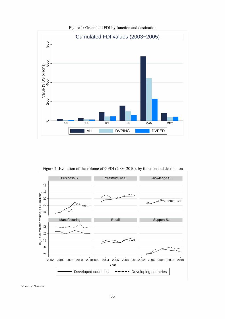
Figure 1: Greenfield FDI by function and destination

020

040

060

080

0V

alue

($

US

bill

ions

)

BS SS KS IS MAN RET

Cumulated FDI values (2003−2005)

ALL DVPING DVPED

Figure 2: Evolution of the volume of GFDI (2003-2010), by function and destination

89

1011

128

910

1112

2002 2004 2006 2008 20102002 2004 2006 2008 20102002 2004 2006 2008 2010

Business S. Infrastructure S. Knowledge S.

Manufacturing Retail Support S.

Developed countries Developing countries

Year

ln(F

DI c

umul

ated

val

ues,

$ U

S m

illio

ns)

Notes: S: Services.

33

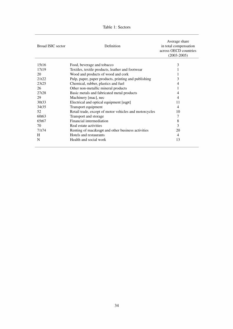
Table 1: Sectors

Average shareBroad ISIC sector Definition in total compensation

across OECD countries(2003-2005)

15t16 Food, beverage and tobacco 317t19 Textiles, textile products, leather and footwear 120 Wood and products of wood and cork 121t22 Pulp, paper, paper products, printing and publishing 323t25 Chemical, rubber, plastics and fuel 426 Other non-metallic mineral products 127t28 Basic metals and fabricated metal products 429 Machinery [mac], nec 430t33 Electrical and optical equipment [eqpt] 1134t35 Transport equipment 452 Retail trade, except of motor vehicles and motorcycles 1060t63 Transport and storage 765t67 Financial intermediation 870 Real estate activities 371t74 Renting of mac&eqpt and other business activities 20H Hotels and restaurants 4N Health and social work 13

34

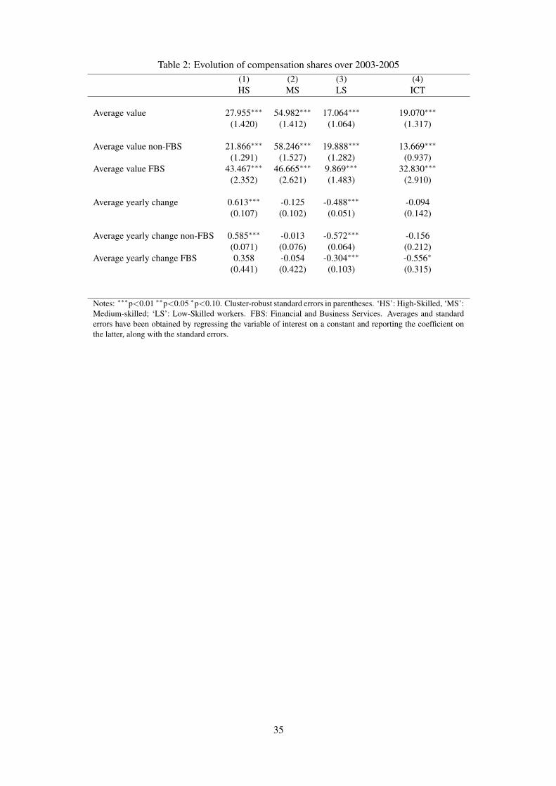
Table 2: Evolution of compensation shares over 2003-2005(1) (2) (3) (4)HS MS LS ICT

Average value 27.955∗∗∗ 54.982∗∗∗ 17.064∗∗∗ 19.070∗∗∗

(1.420) (1.412) (1.064) (1.317)

Average value non-FBS 21.866∗∗∗ 58.246∗∗∗ 19.888∗∗∗ 13.669∗∗∗

(1.291) (1.527) (1.282) (0.937)Average value FBS 43.467∗∗∗ 46.665∗∗∗ 9.869∗∗∗ 32.830∗∗∗

(2.352) (2.621) (1.483) (2.910)

Average yearly change 0.613∗∗∗ -0.125 -0.488∗∗∗ -0.094(0.107) (0.102) (0.051) (0.142)

Average yearly change non-FBS 0.585∗∗∗ -0.013 -0.572∗∗∗ -0.156(0.071) (0.076) (0.064) (0.212)

Average yearly change FBS 0.358 -0.054 -0.304∗∗∗ -0.556∗

(0.441) (0.422) (0.103) (0.315)

Notes: ∗∗∗p<0.01 ∗∗p<0.05 ∗p<0.10. Cluster-robust standard errors in parentheses. ‘HS’: High-Skilled, ‘MS’:Medium-skilled; ‘LS’: Low-Skilled workers. FBS: Financial and Business Services. Averages and standarderrors have been obtained by regressing the variable of interest on a constant and reporting the coefficient onthe latter, along with the standard errors.

35

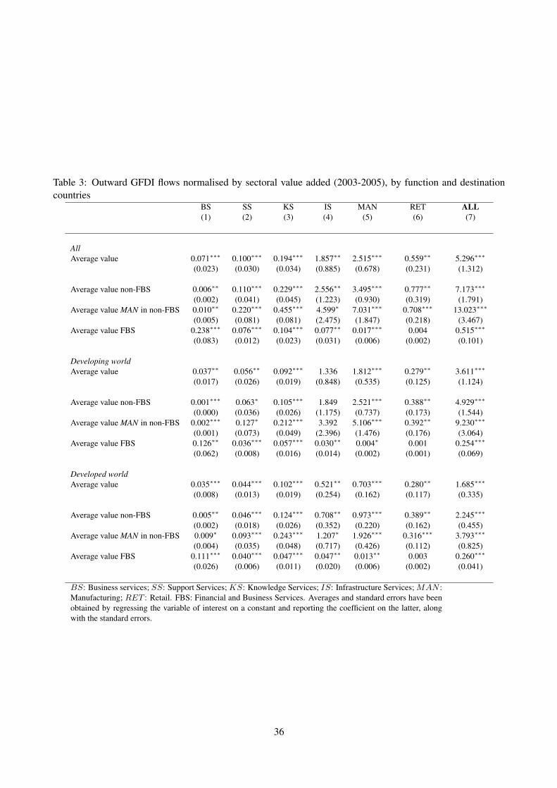
Table 3: Outward GFDI flows normalised by sectoral value added (2003-2005), by function and destinationcountries

BS SS KS IS MAN RET ALL(1) (2) (3) (4) (5) (6) (7)

AllAverage value 0.071∗∗∗ 0.100∗∗∗ 0.194∗∗∗ 1.857∗∗ 2.515∗∗∗ 0.559∗∗ 5.296∗∗∗

(0.023) (0.030) (0.034) (0.885) (0.678) (0.231) (1.312)

Average value non-FBS 0.006∗∗ 0.110∗∗∗ 0.229∗∗∗ 2.556∗∗ 3.495∗∗∗ 0.777∗∗ 7.173∗∗∗

(0.002) (0.041) (0.045) (1.223) (0.930) (0.319) (1.791)Average value MAN in non-FBS 0.010∗∗ 0.220∗∗∗ 0.455∗∗∗ 4.599∗ 7.031∗∗∗ 0.708∗∗∗ 13.023∗∗∗

(0.005) (0.081) (0.081) (2.475) (1.847) (0.218) (3.467)Average value FBS 0.238∗∗∗ 0.076∗∗∗ 0.104∗∗∗ 0.077∗∗ 0.017∗∗∗ 0.004 0.515∗∗∗

(0.083) (0.012) (0.023) (0.031) (0.006) (0.002) (0.101)

Developing worldAverage value 0.037∗∗ 0.056∗∗ 0.092∗∗∗ 1.336 1.812∗∗∗ 0.279∗∗ 3.611∗∗∗

(0.017) (0.026) (0.019) (0.848) (0.535) (0.125) (1.124)

Average value non-FBS 0.001∗∗∗ 0.063∗ 0.105∗∗∗ 1.849 2.521∗∗∗ 0.388∗∗ 4.929∗∗∗

(0.000) (0.036) (0.026) (1.175) (0.737) (0.173) (1.544)Average value MAN in non-FBS 0.002∗∗∗ 0.127∗ 0.212∗∗∗ 3.392 5.106∗∗∗ 0.392∗∗ 9.230∗∗∗

(0.001) (0.073) (0.049) (2.396) (1.476) (0.176) (3.064)Average value FBS 0.126∗∗ 0.036∗∗∗ 0.057∗∗∗ 0.030∗∗ 0.004∗ 0.001 0.254∗∗∗

(0.062) (0.008) (0.016) (0.014) (0.002) (0.001) (0.069)

Developed worldAverage value 0.035∗∗∗ 0.044∗∗∗ 0.102∗∗∗ 0.521∗∗ 0.703∗∗∗ 0.280∗∗ 1.685∗∗∗

(0.008) (0.013) (0.019) (0.254) (0.162) (0.117) (0.335)

Average value non-FBS 0.005∗∗ 0.046∗∗∗ 0.124∗∗∗ 0.708∗∗ 0.973∗∗∗ 0.389∗∗ 2.245∗∗∗

(0.002) (0.018) (0.026) (0.352) (0.220) (0.162) (0.455)Average value MAN in non-FBS 0.009∗ 0.093∗∗∗ 0.243∗∗∗ 1.207∗ 1.926∗∗∗ 0.316∗∗∗ 3.793∗∗∗

(0.004) (0.035) (0.048) (0.717) (0.426) (0.112) (0.825)Average value FBS 0.111∗∗∗ 0.040∗∗∗ 0.047∗∗∗ 0.047∗∗ 0.013∗∗ 0.003 0.260∗∗∗

(0.026) (0.006) (0.011) (0.020) (0.006) (0.002) (0.041)

BS: Business services; SS: Support Services; KS: Knowledge Services; IS: Infrastructure Services; MAN :Manufacturing; RET : Retail. FBS: Financial and Business Services. Averages and standard errors have beenobtained by regressing the variable of interest on a constant and reporting the coefficient on the latter, alongwith the standard errors.

36

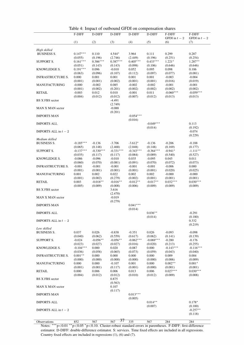
Table 4: Impact of outbound GFDI on compensation sharesF-DIFF D-DIFF D-DIFF D-DIFF D-DIFF F-DIFF F-DIFF

GFDI in t− 2 GFDI in t− 2(1) (2) (3) (4) (5) (6) (7)

High skilledBUSINESS S. 0.147∗∗∗ 0.110 4.544∗ 3.964 0.111 0.299 0.287

(0.055) (0.196) (2.746) (2.449) (0.196) (0.251) (0.254)SUPPORT S. 0.161∗∗∗ 0.386∗∗∗ 0.387∗∗∗ 0.405∗∗∗ 0.433∗∗∗ 1.221∗ 1.287∗∗

(0.051) (0.143) (0.143) (0.098) (0.106) (0.646) (0.646)KNOWLEDGE S. 0.191∗∗∗ 0.096 -0.010 0.052 0.095 0.098 0.106

(0.063) (0.096) (0.107) (0.112) (0.097) (0.077) (0.081)INFRASTRUCTURE S. 0.000 0.001 0.001 0.001 0.001 -0.003 -0.004

(0.001) (0.001) (0.002) (0.001) (0.001) (0.016) (0.019)MANUFACTURING -0.000 -0.002 0.085 -0.002 -0.002 -0.001 -0.001

(0.001) (0.002) (0.201) (0.002) (0.002) (0.002) (0.002)RETAIL -0.003 0.012 0.010 -0.001 0.011 -0.060∗∗∗ -0.059∗∗∗

(0.004) (0.012) (0.012) (0.007) (0.012) (0.013) (0.013)BS X FBS sector -4.491

(2.749)MAN X MAN sector -0.088

(0.201)IMPORTS MAN -0.054∗∗∗

(0.016)IMPORTS ALL -0.049∗∗∗ 0.113

(0.014) (0.192)IMPORTS ALL in t− 2 -0.074

(0.229)Medium skilledBUSINESS S. -0.185∗∗∗ -0.136 -3.706 -3.612∗ -0.136 -0.206 -0.188

(0.065) (0.148) (2.468) (2.048) (0.148) (0.169) (0.177)SUPPORT S. -0.137∗∗∗ -0.330∗∗∗ -0.331∗∗∗ -0.343∗∗∗ -0.364∗∗∗ -0.941∗ -1.111∗∗

(0.035) (0.117) (0.117) (0.084) (0.089) (0.540) (0.527)KNOWLEDGE S. -0.086 -0.096 -0.010 0.035 -0.095 0.045 0.011

(0.060) (0.070) (0.081) (0.091) (0.070) (0.072) (0.073)INFRASTRUCTURE S. -0.001 -0.001 -0.001 -0.001 -0.001 -0.006 0.000

(0.001) (0.001) (0.001) (0.001) (0.001) (0.020) (0.025)MANUFACTURING 0.001 0.002 0.022 0.002 0.002 -0.000 -0.000

(0.001) (0.002) (0.279) (0.002) (0.001) (0.001) (0.001)RETAIL 0.003 -0.018∗∗ -0.016∗∗ -0.012∗∗ -0.017∗∗ 0.032∗∗∗ 0.030∗∗∗

(0.005) (0.009) (0.008) (0.006) (0.009) (0.009) (0.009)BS X FBS sector 3.616

(2.470)MAN X MAN sector -0.019

(0.279)IMPORTS MAN 0.041∗∗∗

(0.014)IMPORTS ALL 0.036∗∗ -0.291

(0.014) (0.180)IMPORTS ALL in t− 2 0.332

(0.219)Low skilledBUSINESS S. 0.037 0.026 -0.838 -0.351 0.026 -0.093 -0.098

(0.040) (0.062) (0.559) (0.617) (0.062) (0.141) (0.139)SUPPORT S. -0.024 -0.056∗∗ -0.056∗∗ -0.062∗∗∗ -0.069∗∗∗ -0.280 -0.176

(0.023) (0.027) (0.027) (0.016) (0.020) (0.213) (0.255)KNOWLEDGE S. -0.104∗∗∗ 0.000 0.020 -0.087 0.000 -0.143∗∗∗ -0.116∗∗∗

(0.036) (0.058) (0.065) (0.073) (0.059) (0.043) (0.040)INFRASTRUCTURE S. 0.001∗∗ 0.000 0.000 0.000 0.000 0.009 0.004

(0.000) (0.000) (0.000) (0.000) (0.000) (0.006) (0.009)MANUFACTURING 0.000 0.000 -0.107 0.001 0.000 0.002∗∗ 0.001∗

(0.001) (0.001) (0.117) (0.001) (0.000) (0.001) (0.001)RETAIL 0.000 0.006 0.006 0.013 0.006 0.027∗∗∗ 0.030∗∗∗

(0.004) (0.012) (0.012) (0.010) (0.012) (0.009) (0.008)BS X FBS sector 0.875

(0.563)MAN X MAN sector 0.107

(0.117)IMPORTS MAN 0.013∗∗∗

(0.005)IMPORTS ALL 0.014∗∗ 0.178∗

(0.007) (0.100)IMPORTS ALL in t− 2 -0.257∗∗

(0.118)

Observations 852 567 567 335 567 284 284Notes: ∗∗∗p<0.01 ∗∗p<0.05 ∗p<0.10. Cluster-robust standard errors in parentheses. F-DIFF: first-differenceestimator. D-DIFF: double-difference estimator. S: services. Time fixed effects are included in all regressions.Country fixed effects are included in regressions (1), (6) and (7).

37

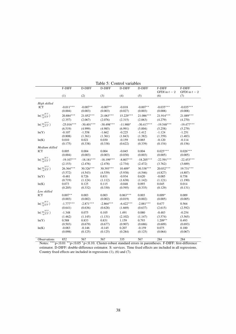
Table 5: Control variablesF-DIFF D-DIFF D-DIFF D-DIFF D-DIFF F-DIFF F-DIFF

GFDI in t− 2 GFDI in t− 2(1) (2) (3) (4) (5) (6) (7)

High skilledICT -0.011∗∗∗ -0.007∗∗ -0.007∗∗ -0.018 -0.007∗∗ -0.035∗∗∗ -0.035∗∗∗

(0.004) (0.003) (0.003) (0.027) (0.003) (0.008) (0.008)

ln(wHS

wLS ) 20.884∗∗∗ 21.052∗∗∗ 21.063∗∗∗ 15.229∗∗∗ 21.086∗∗∗ 21.914∗∗∗ 21.889∗∗∗

(2.357) (2.067) (2.076) (2.315) (2.063) (4.279) (4.270)

ln(wMS

wLS ) -25.016∗∗∗ -30.401∗∗∗ -30.498∗∗∗ -11.900∗ -30.417∗∗∗ -19.548∗∗∗ -19.477∗∗∗

(6.519) (4.999) (4.985) (6.991) (5.004) (5.258) (5.279)ln(Y) -0.107 -1.558 -1.662 -0.225 -1.412 -1.124 -1.251

(0.808) (1.361) (1.361) (1.843) (1.382) (1.359) (1.483)ln(K) 0.010 0.021 0.030 -0.159 0.065 -0.120 -0.114

(0.175) (0.338) (0.338) (0.622) (0.339) (0.154) (0.156)Medium skilledICT 0.005 0.004 0.004 -0.045 0.004 0.025∗∗∗ 0.026∗∗∗

(0.004) (0.003) (0.003) (0.030) (0.003) (0.005) (0.005)

ln(wHS

wLS ) -19.107∗∗∗ -18.181∗∗∗ -18.199∗∗∗ -8.807∗∗∗ -18.205∗∗∗ -22.591∗∗∗ -22.453∗∗∗

(2.153) (2.476) (2.478) (2.734) (2.472) (3.762) (3.689)

ln(wMS

wLS ) 26.364∗∗∗ 30.326∗∗∗ 30.393∗∗∗ 10.409∗ 30.338∗∗∗ 20.032∗∗∗ 19.731∗∗∗

(5.572) (4.543) (4.539) (5.938) (4.546) (4.827) (4.807)ln(Y) -0.481 0.726 0.831 -0.934 0.620 -0.085 0.758

(0.719) (1.124) (1.112) (1.638) (1.142) (1.121) (1.190)ln(K) 0.073 0.125 0.115 -0.048 0.093 0.045 0.014

(0.205) (0.332) (0.330) (0.595) (0.335) (0.129) (0.131)Low skilledICT 0.007∗∗ 0.003 0.003 0.063∗∗∗ 0.003 0.009∗ 0.009

(0.003) (0.002) (0.002) (0.019) (0.002) (0.005) (0.005)

ln(wHS

wLS ) -1.777∗∗∗ -2.871∗∗∗ -2.864∗∗∗ -6.422∗∗∗ -2.881∗∗∗ 0.677 0.564(0.641) (0.636) (0.628) (1.669) (0.637) (2.615) (2.592)

ln(wMS

wLS ) -1.348 0.075 0.105 1.491 0.080 -0.483 -0.254(1.462) (1.145) (1.131) (2.102) (1.147) (3.574) (3.565)

ln(Y) 0.588 0.833 0.831 1.159 0.793 1.209∗∗ 0.493(0.503) (0.679) (0.677) (0.907) (0.686) (0.609) (0.693)

ln(K) -0.083 -0.146 -0.145 0.207 -0.159 0.075 0.100(0.098) (0.125) (0.125) (0.284) (0.125) (0.064) (0.067)

Observations 852 567 567 335 567 284 284Notes: ∗∗∗p<0.01 ∗∗p<0.05 ∗p<0.10. Cluster-robust standard errors in parentheses. F-DIFF: first-differenceestimator. D-DIFF: double-difference estimator. S: services. Time fixed effects are included in all regressions.Country fixed effects are included in regressions (1), (6) and (7).

38

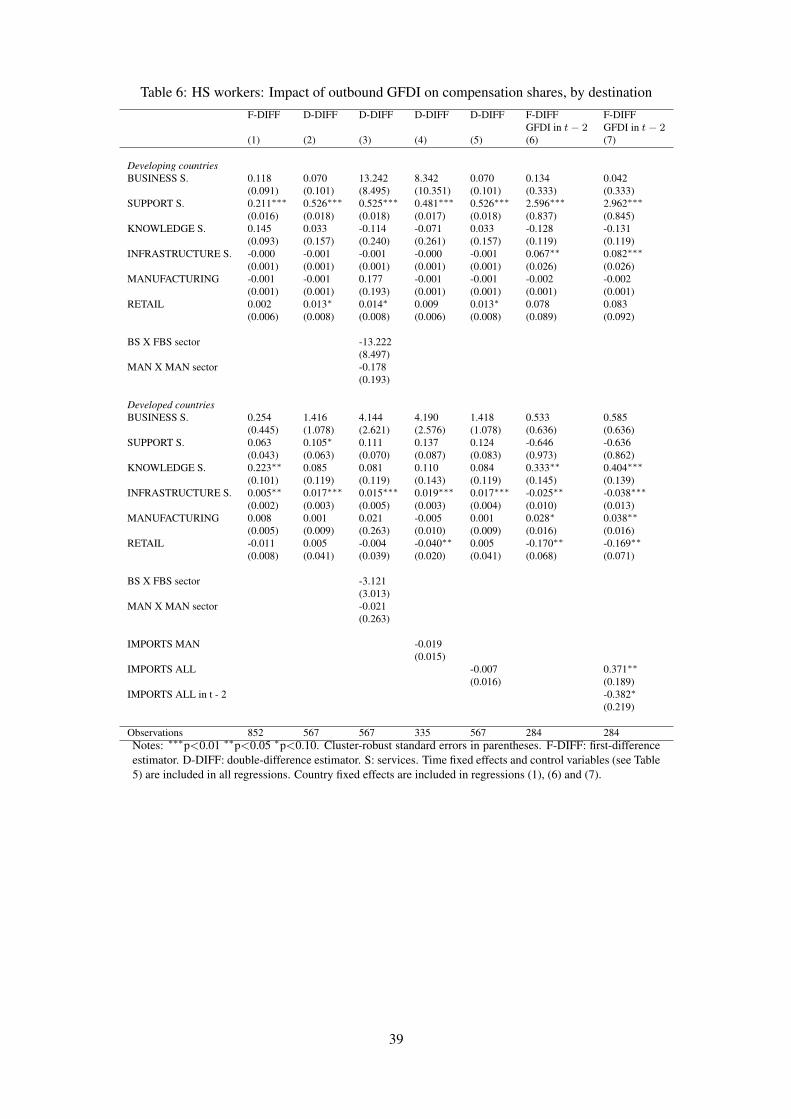
Table 6: HS workers: Impact of outbound GFDI on compensation shares, by destinationF-DIFF D-DIFF D-DIFF D-DIFF D-DIFF F-DIFF F-DIFF

GFDI in t− 2 GFDI in t− 2(1) (2) (3) (4) (5) (6) (7)

Developing countriesBUSINESS S. 0.118 0.070 13.242 8.342 0.070 0.134 0.042

(0.091) (0.101) (8.495) (10.351) (0.101) (0.333) (0.333)SUPPORT S. 0.211∗∗∗ 0.526∗∗∗ 0.525∗∗∗ 0.481∗∗∗ 0.526∗∗∗ 2.596∗∗∗ 2.962∗∗∗

(0.016) (0.018) (0.018) (0.017) (0.018) (0.837) (0.845)KNOWLEDGE S. 0.145 0.033 -0.114 -0.071 0.033 -0.128 -0.131

(0.093) (0.157) (0.240) (0.261) (0.157) (0.119) (0.119)INFRASTRUCTURE S. -0.000 -0.001 -0.001 -0.000 -0.001 0.067∗∗ 0.082∗∗∗

(0.001) (0.001) (0.001) (0.001) (0.001) (0.026) (0.026)MANUFACTURING -0.001 -0.001 0.177 -0.001 -0.001 -0.002 -0.002

(0.001) (0.001) (0.193) (0.001) (0.001) (0.001) (0.001)RETAIL 0.002 0.013∗ 0.014∗ 0.009 0.013∗ 0.078 0.083

(0.006) (0.008) (0.008) (0.006) (0.008) (0.089) (0.092)

BS X FBS sector -13.222(8.497)

MAN X MAN sector -0.178(0.193)

Developed countriesBUSINESS S. 0.254 1.416 4.144 4.190 1.418 0.533 0.585

(0.445) (1.078) (2.621) (2.576) (1.078) (0.636) (0.636)SUPPORT S. 0.063 0.105∗ 0.111 0.137 0.124 -0.646 -0.636

(0.043) (0.063) (0.070) (0.087) (0.083) (0.973) (0.862)KNOWLEDGE S. 0.223∗∗ 0.085 0.081 0.110 0.084 0.333∗∗ 0.404∗∗∗

(0.101) (0.119) (0.119) (0.143) (0.119) (0.145) (0.139)INFRASTRUCTURE S. 0.005∗∗ 0.017∗∗∗ 0.015∗∗∗ 0.019∗∗∗ 0.017∗∗∗ -0.025∗∗ -0.038∗∗∗

(0.002) (0.003) (0.005) (0.003) (0.004) (0.010) (0.013)MANUFACTURING 0.008 0.001 0.021 -0.005 0.001 0.028∗ 0.038∗∗

(0.005) (0.009) (0.263) (0.010) (0.009) (0.016) (0.016)RETAIL -0.011 0.005 -0.004 -0.040∗∗ 0.005 -0.170∗∗ -0.169∗∗

(0.008) (0.041) (0.039) (0.020) (0.041) (0.068) (0.071)

BS X FBS sector -3.121(3.013)

MAN X MAN sector -0.021(0.263)

IMPORTS MAN -0.019(0.015)

IMPORTS ALL -0.007 0.371∗∗

(0.016) (0.189)IMPORTS ALL in t - 2 -0.382∗

(0.219)

Observations 852 567 567 335 567 284 284Notes: ∗∗∗p<0.01 ∗∗p<0.05 ∗p<0.10. Cluster-robust standard errors in parentheses. F-DIFF: first-differenceestimator. D-DIFF: double-difference estimator. S: services. Time fixed effects and control variables (see Table5) are included in all regressions. Country fixed effects are included in regressions (1), (6) and (7).

39

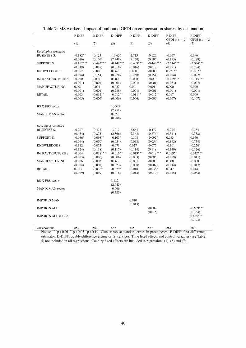
Table 7: MS workers: Impact of outbound GFDI on compensation shares, by destinationF-DIFF D-DIFF D-DIFF D-DIFF D-DIFF F-DIFF F-DIFF

GFDI in t− 2 GFDI in t− 2(1) (2) (3) (4) (5) (6) (7)

Developing countriesBUSINESS S. -0.182∗∗ -0.123 -10.655 -2.713 -0.123 -0.057 0.096

(0.086) (0.105) (7.748) (9.130) (0.105) (0.195) (0.188)SUPPORT S. -0.162∗∗∗ -0.443∗∗∗ -0.442∗∗∗ -0.409∗∗∗ -0.443∗∗∗ -2.514∗∗∗ -3.074∗∗∗

(0.019) (0.018) (0.018) (0.016) (0.018) (0.791) (0.784)KNOWLEDGE S. -0.052 -0.080 0.069 0.080 -0.080 0.221∗∗ 0.221∗∗

(0.094) (0.154) (0.228) (0.250) (0.154) (0.094) (0.092)INFRASTRUCTURE S. -0.000 0.000 0.000 -0.000 0.000 -0.089∗∗∗ -0.115∗∗∗

(0.001) (0.001) (0.001) (0.001) (0.001) (0.033) (0.027)MANUFACTURING 0.001 0.001 -0.027 0.001 0.001 0.000 0.000

(0.001) (0.001) (0.288) (0.001) (0.001) (0.001) (0.001)RETAIL -0.003 -0.012∗∗ -0.012∗∗ -0.011∗∗ -0.012∗∗ 0.017 0.009

(0.005) (0.006) (0.006) (0.006) (0.006) (0.097) (0.107)

BS X FBS sector 10.577(7.751)

MAN X MAN sector 0.029(0.288)

Developed countriesBUSINESS S. -0.207 -0.477 -3.217 -3.663 -0.477 -0.275 -0.384

(0.434) (0.873) (2.366) (2.363) (0.874) (0.341) (0.338)SUPPORT S. -0.086∗ -0.098∗∗ -0.103∗ -0.108 -0.092∗ 0.983 0.970

(0.044) (0.050) (0.054) (0.068) (0.054) (0.862) (0.734)KNOWLEDGE S. -0.112 -0.075 -0.071 0.027 -0.075 -0.101 -0.220∗

(0.124) (0.118) (0.117) (0.114) (0.118) (0.149) (0.126)INFRASTRUCTURE S. -0.004 -0.018∗∗∗ -0.016∗∗ -0.019∗∗∗ -0.018∗∗∗ 0.019∗∗ 0.042∗∗∗

(0.003) (0.005) (0.006) (0.003) (0.005) (0.009) (0.011)MANUFACTURING -0.006 -0.003 0.063 -0.001 -0.003 0.008 -0.008

(0.004) (0.007) (0.323) (0.008) (0.007) (0.014) (0.017)RETAIL 0.013 -0.036∗ -0.029∗ -0.018 -0.036∗ 0.047 0.044

(0.009) (0.019) (0.018) (0.014) (0.019) (0.075) (0.084)

BS X FBS sector 3.132(2.645)

MAN X MAN sector -0.066(0.323)

IMPORTS MAN 0.010(0.013)

IMPORTS ALL -0.002 -0.569∗∗∗

(0.015) (0.164)IMPORTS ALL in t - 2 0.665∗∗∗

(0.193)

Observations 852 567 567 335 567 284 284Notes: ∗∗∗p<0.01 ∗∗p<0.05 ∗p<0.10. Cluster-robust standard errors in parentheses. F-DIFF: first-differenceestimator. D-DIFF: double-difference estimator. S: services. Time fixed effects and control variables (see Table5) are included in all regressions. Country fixed effects are included in regressions (1), (6) and (7).

40

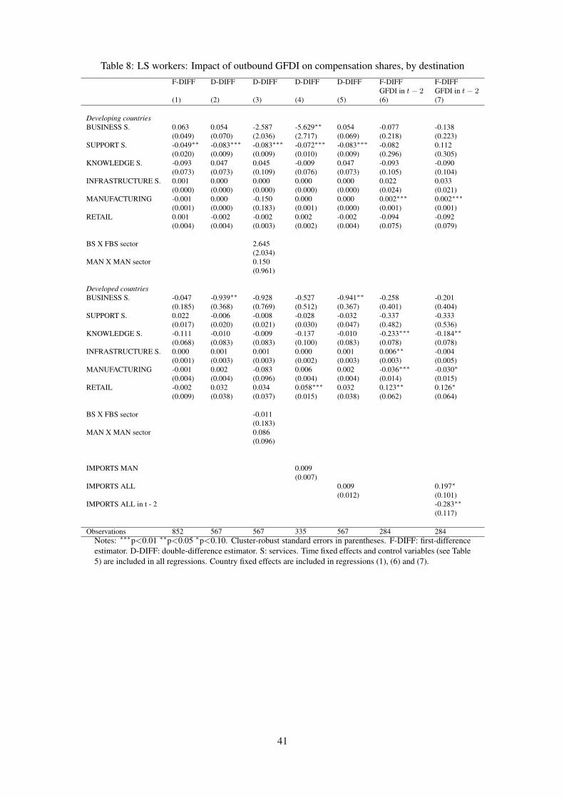
Table 8: LS workers: Impact of outbound GFDI on compensation shares, by destinationF-DIFF D-DIFF D-DIFF D-DIFF D-DIFF F-DIFF F-DIFF

GFDI in t− 2 GFDI in t− 2(1) (2) (3) (4) (5) (6) (7)

Developing countriesBUSINESS S. 0.063 0.054 -2.587 -5.629∗∗ 0.054 -0.077 -0.138

(0.049) (0.070) (2.036) (2.717) (0.069) (0.218) (0.223)SUPPORT S. -0.049∗∗ -0.083∗∗∗ -0.083∗∗∗ -0.072∗∗∗ -0.083∗∗∗ -0.082 0.112

(0.020) (0.009) (0.009) (0.010) (0.009) (0.296) (0.305)KNOWLEDGE S. -0.093 0.047 0.045 -0.009 0.047 -0.093 -0.090

(0.073) (0.073) (0.109) (0.076) (0.073) (0.105) (0.104)INFRASTRUCTURE S. 0.001 0.000 0.000 0.000 0.000 0.022 0.033

(0.000) (0.000) (0.000) (0.000) (0.000) (0.024) (0.021)MANUFACTURING -0.001 0.000 -0.150 0.000 0.000 0.002∗∗∗ 0.002∗∗∗

(0.001) (0.000) (0.183) (0.001) (0.000) (0.001) (0.001)RETAIL 0.001 -0.002 -0.002 0.002 -0.002 -0.094 -0.092

(0.004) (0.004) (0.003) (0.002) (0.004) (0.075) (0.079)

BS X FBS sector 2.645(2.034)

MAN X MAN sector 0.150(0.961)

Developed countriesBUSINESS S. -0.047 -0.939∗∗ -0.928 -0.527 -0.941∗∗ -0.258 -0.201

(0.185) (0.368) (0.769) (0.512) (0.367) (0.401) (0.404)SUPPORT S. 0.022 -0.006 -0.008 -0.028 -0.032 -0.337 -0.333

(0.017) (0.020) (0.021) (0.030) (0.047) (0.482) (0.536)KNOWLEDGE S. -0.111 -0.010 -0.009 -0.137 -0.010 -0.233∗∗∗ -0.184∗∗

(0.068) (0.083) (0.083) (0.100) (0.083) (0.078) (0.078)INFRASTRUCTURE S. 0.000 0.001 0.001 0.000 0.001 0.006∗∗ -0.004

(0.001) (0.003) (0.003) (0.002) (0.003) (0.003) (0.005)MANUFACTURING -0.001 0.002 -0.083 0.006 0.002 -0.036∗∗∗ -0.030∗

(0.004) (0.004) (0.096) (0.004) (0.004) (0.014) (0.015)RETAIL -0.002 0.032 0.034 0.058∗∗∗ 0.032 0.123∗∗ 0.126∗

(0.009) (0.038) (0.037) (0.015) (0.038) (0.062) (0.064)

BS X FBS sector -0.011(0.183)

MAN X MAN sector 0.086(0.096)

IMPORTS MAN 0.009(0.007)

IMPORTS ALL 0.009 0.197∗

(0.012) (0.101)IMPORTS ALL in t - 2 -0.283∗∗

(0.117)

Observations 852 567 567 335 567 284 284Notes: ∗∗∗p<0.01 ∗∗p<0.05 ∗p<0.10. Cluster-robust standard errors in parentheses. F-DIFF: first-differenceestimator. D-DIFF: double-difference estimator. S: services. Time fixed effects and control variables (see Table5) are included in all regressions. Country fixed effects are included in regressions (1), (6) and (7).

41

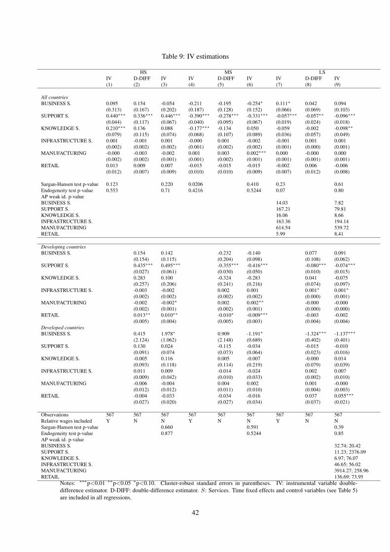
Table 9: IV estimations

HS MS LSIV D-DIFF IV IV D-DIFF IV IV D-DIFF IV(1) (2) (3) (4) (5) (6) (7) (8) (9)

All countriesBUSINESS S. 0.095 0.154 -0.054 -0.211 -0.195 -0.254∗ 0.111∗ 0.042 0.094

(0.313) (0.167) (0.202) (0.187) (0.128) (0.152) (0.066) (0.069) (0.103)SUPPORT S. 0.440∗∗∗ 0.336∗∗∗ 0.446∗∗∗ -0.390∗∗∗ -0.278∗∗∗ -0.331∗∗∗ -0.057∗∗∗ -0.057∗∗ -0.096∗∗∗

(0.044) (0.117) (0.067) (0.040) (0.095) (0.067) (0.019) (0.024) (0.018)KNOWLEDGE S. 0.210∗∗∗ 0.136 0.088 -0.177∗∗∗ -0.134 0.050 -0.059 -0.002 -0.098∗∗

(0.079) (0.115) (0.074) (0.068) (0.107) (0.089) (0.036) (0.057) (0.049)INFRASTRUCTURE S. 0.001 -0.001 0.001 -0.000 0.001 -0.002 -0.001 0.001 0.001

(0.002) (0.002) (0.002) (0.001) (0.002) (0.002) (0.001) (0.000) (0.001)MANUFACTURING -0.000 -0.003 -0.002 0.001 0.003 0.002∗∗∗ 0.000 -0.000 0.000

(0.002) (0.002) (0.001) (0.001) (0.002) (0.001) (0.001) (0.001) (0.001)RETAIL 0.013 0.009 0.007 -0.015 -0.015 -0.015 -0.002 0.006 -0.006

(0.012) (0.007) (0.009) (0.010) (0.010) (0.009) (0.007) (0.012) (0.008)

Sargan-Hansen test p-value 0.123 0.220 0.0206 0.410 0.23 0.61Endogeneity test p-value 0.553 0.71 0.4216 0.5244 0.07 0.80AP weak id. p-valueBUSINESS S. 14.03 7.82SUPPORT S. 167.21 79.81KNOWLEDGE S. 16.06 8.66INFRASTRUCTURE S. 163.36 194.14MANUFACTURING 614.54 539.72RETAIL 5.99 8.41

Developing countriesBUSINESS S. 0.154 0.142 -0.232 -0.140 0.077 0.091

(0.154) (0.115) (0.204) (0.098) (0.108) (0.062)SUPPORT S. 0.435∗∗∗ 0.495∗∗∗ -0.355∗∗∗ -0.416∗∗∗ -0.080∗∗∗ -0.074∗∗∗

(0.027) (0.061) (0.030) (0.050) (0.010) (0.015)KNOWLEDGE S. 0.283 0.100 -0.324 -0.283 0.041 -0.075

(0.257) (0.206) (0.241) (0.216) (0.074) (0.097)INFRASTRUCTURE S. -0.003 -0.002 0.002 0.001 0.001∗ 0.001∗

(0.002) (0.002) (0.002) (0.002) (0.000) (0.001)MANUFACTURING -0.002 -0.002∗ 0.002 0.002∗∗ -0.000 -0.000

(0.002) (0.001) (0.002) (0.001) (0.000) (0.000)RETAIL 0.013∗∗ 0.010∗∗ -0.010∗ -0.009∗∗∗ -0.003 -0.002

(0.005) (0.004) (0.005) (0.003) (0.004) (0.004)Developed countriesBUSINESS S. 0.415 1.978∗ 0.909 -1.191∗ -1.324∗∗∗ -1.137∗∗∗

(2.124) (1.062) (2.148) (0.689) (0.402) (0.401)SUPPORT S. 0.130 0.024 -0.115 -0.034 -0.015 -0.010

(0.091) (0.074 (0.073) (0.064) (0.023) (0.016)KNOWLEDGE S. -0.005 0.116 0.005 -0.007 -0.000 0.014

(0.093) (0.118) (0.114) (0.219) (0.079) (0.039)INFRASTRUCTURE S. 0.011 0.009 -0.014 -0.024 0.002 0.007

(0.009) (0.042) (0.010) (0.033) (0.002) (0.010)MANUFACTURING -0.006 -0.004 0.004 0.002 0.001 -0.000

(0.012) (0.012) (0.011) (0.010) (0.004) (0.003)RETAIL -0.004 -0.033 -0.034 -0.016 0.037 0.055∗∗∗

(0.027) (0.020) (0.027) (0.034) (0.037) (0.021)

Observations 567 567 567 567 567 567 567 567 567Relative wages included Y N N Y N N Y N NSargan-Hansen test p-value 0.660 0.591 0.39Endogeneity test p-value 0.877 0.5244 0.85AP weak id. p-valueBUSINESS S. 32.74; 20.42SUPPORT S. 11.23; 2376.09KNOWLEDGE S. 6.97; 76.07INFRASTRUCTURE S. 46.65; 56.02MANUFACTURING 3914.27; 258.96RETAIL 136.69; 73.95

Notes: ∗∗∗p<0.01 ∗∗p<0.05 ∗p<0.10. Cluster-robust standard errors in parentheses. IV: instrumental variable double-difference estimator. D-DIFF: double-difference estimator. S: Services. Time fixed effects and control variables (see Table 5)are included in all regressions.

42

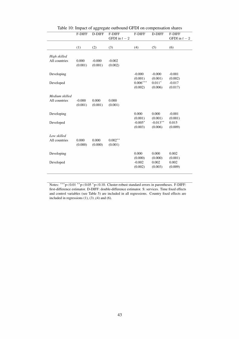
Table 10: Impact of aggregate outbound GFDI on compensation sharesF-DIFF D-DIFF F-DIFF F-DIFF D-DIFF F-DIFF

GFDI in t− 2 GFDI in t− 2

(1) (2) (3) (4) (5) (6)

High skilledAll countries 0.000 -0.000 -0.002

(0.001) (0.001) (0.002)

Developing -0.000 -0.000 -0.001(0.001) (0.001) (0.002)

Developed 0.006∗∗∗ 0.011∗ -0.017(0.002) (0.006) (0.017)

Medium skilledAll countries -0.000 0.000 0.000

(0.001) (0.001) (0.001)

Developing 0.000 0.000 -0.001(0.001) (0.001) (0.001)

Developed -0.005∗ -0.013∗∗ 0.015(0.003) (0.006) (0.009)

Low skilledAll countries 0.000 0.000 0.002∗∗

(0.000) (0.000) (0.001)

Developing 0.000 0.000 0.002(0.000) (0.000) (0.001)

Developed -0.002 0.002 0.002(0.002) (0.003) (0.009)

Notes: ∗∗∗p<0.01 ∗∗p<0.05 ∗p<0.10. Cluster-robust standard errors in parentheses. F-DIFF:first-difference estimator. D-DIFF: double-difference estimator. S: services. Time fixed effectsand control variables (see Table 5) are included in all regressions. Country fixed effects areincluded in regressions (1), (3) ,(4) and (6).

43