Embed Size (px)
DESCRIPTION
Gregory Smith Dissertation
Citation preview

A Deterministic Approach to Partitioning Neural Network Training Data for the Classification Problem
Gregory E. Smith
Dissertation submitted to the Faculty of Virginia Polytechnic Institute & State University
in partial fulfillment of the requirements for the degree of Doctor of Philosophy
in Business; Management Science
Dr. Cliff T. Ragsdale, Chairman Dr. Evelyn C. Brown Dr. Deborah F. Cook
Dr. Loren P. Rees Dr. Christopher W. Zobel
August 7, 2006 Blacksburg, Virginia
Keywords: Neural Networks, Discriminant Analysis, Convex Sets, Data Partitioning
Copyright 2006, Gregory E. Smith
ALL RIGHTS RESERVED

A Deterministic Approach to Partitioning Neural Network Training Data for the Classification Problem
Gregory E. Smith
(ABSTRACT)
The classification problem in discriminant analysis involves identifying a function that accurately
classifies observations as originating from one of two or more mutually exclusive groups. Because no
single classification technique works best for all problems, many different techniques have been
developed. For business applications, neural networks have become the most commonly used
classification technique and though they often outperform traditional statistical classification methods,
their performance may be hindered because of failings in the use of training data. This problem can be
exacerbated because of small data set size.
In this dissertation, we identify and discuss a number of potential problems with typical random
partitioning of neural network training data for the classification problem and introduce deterministic
methods to partitioning that overcome these obstacles and improve classification accuracy on new
validation data. A traditional statistical distance measure enables this deterministic partitioning.
Heuristics for both the two-group classification problem and k-group classification problem are presented.
We show that these heuristics result in generalizable neural network models that produce more accurate
classification results, on average, than several commonly used classification techniques.
In addition, we compare several two-group simulated and real-world data sets with respect to the
interior and boundary positions of observations within their groups’ convex polyhedrons. We show by
example that projecting the interior points of simulated data to the boundary of their group polyhedrons
generates convex shapes similar to real-world data group convex polyhedrons. Our two-group
deterministic partitioning heuristic is then applied to the repositioned simulated data, producing results
superior to several commonly used classification techniques.

iii
DEDICATION
I dedicate this work to my wife Julie and to our newborn son Jacob. Julie, you have made this journey possible for me. Your support and constant encouragement helped me through all the highs and lows over the past three years. I love you so very much.
To Jacob, the thought of your arrival gave me the strength to complete my degree. Now that you are with us, I can’t image life without you.

iv
ACKNOWLEDGEMENTS
I would like to extend a work of thanks to Dr. Cliff Ragsdale, my major professor, for the guidance you have provided to me. You have challenged me every step of the way. I can now say that I have seen the very best in action.
Thank you to those who served on my committee: Dr. Loren Rees, Dr. Debbie Cook, Dr. Chris Zobel, and Dr. Evelyn Brown. Thank you for your patience, input, and guidance.
I would also like to thank the late Dr. Earnest Houck for taking a chance on a burned-out actuary from New York. Your risk has been a blessing for me. You are truly missed.
I would like to thank my father, Willis Smith, for your constant availability when “real” work needed to be done.
I would like to thank my Cavalier King Charles Spaniels (Chloe, Ollie, and Leeza) for keeping me company on many long nights of study and writing.
Finally, thank you to my family and friends for all your support.

v
TABLE OF CONTENTS ` CHAPTER 1: INTRODUCTION AND LITERATURE REVIEW……………….. 1
INTRODUCTION…………………………………………………………………...` 2 STATEMENT OF THE PROBLEM………………………………………………... 8 OBJECTIVE OF THE STUDY……………………………………………………... 9 RESEARCH METHODOLOGY……………………………………………………. 9 SCOPE AND LIMITATIONS………………………………………………………. 10 CONTRIBUTIONS OF THE RESEARCH…………………………………………. 11 PLAN OF PRESENTATION………………………………………………………... 11
CHAPTER 2: A DETERMINISTIC APPROACH TO PARTITIONING NEURAL
NETWORK TRAINING DATA FOR THE 2-GROUP CLASSIFICATION PROBLEM……………………………………. 13
1. INTRODUCTION………………………………………………………………….. 14 2. CLASSIFICATION METHODS………………………………………………….. 16
2.1 Mahalanobis Distance Measure…..…………………………………………….. 16 2.2 Neural Networks………………………………………………………………... 17
3. DETERMINISTIC NEURAL NETWORK DATA PARTITIONING………….. 21 4. METHODOLOGY…………………………………………………………………. 22 5. RESULTS…………………………………………………………………………… 25 5.1 Texas Bank Data………………………………………………………………… 25 5.2 Moody’s Industrial Data………………………………………………………… 26
6. IMPLICATIONS AND CONCLUSIONS………………………………………… 28
6.1 Implications…………………………………………………………………….... 28 6.2 Conclusions…………………………………………………………………….... 29
REFERENCES…………………………………………………………………………… 30 CHAPTER 3: A DETERMINISTIC NEURAL NETWORK DATA PARTITIONING
APPROACH TO THE k-GROUP CLASSIFICATION PROBLEM IN DISCRIMINANTANALYSIS……………………………………….. 32
1. INTRODUCTION…………………………………………………………………... 33 2. THE MGCP……………………..…………………………………………………… 36

vi
3. CLASSIFICATION METHODS…………………………………………………... 41 3.1 Mahalanobis Distance Measure….………………………………………………. 41 3.2 Neural Networks…………………………………………………………………. 42
4. DETERMINISTIC NEURAL NETWORK DATA PARTITIONING….……….. 46 4.1 NNDP……………………………………………………………………………... 46 4.2 kNNDP……………………………………………………………………………. 47
5. EXPERIMENTAL DESIGN……………………………………………………….. 50 6. RESULTS……………………………………………………………………………. 54
6.1 Balanced Scale Weight and Distance Data………………………………………. 54 6.2 Contraceptive Prevalence Survey……………………………………………….... 55 6.3 Teaching Assistant Evaluation Data……………………………………………… 56
7. IMPLICATIONS AND CONCLUSIONS…………………………………………. 57
7.1 Implications………………………………………………………………………. 57 7.2 Conclusions………………………………………………………………………. 57
REFERENCES……………………………………………………………………………. 62 CHAPTER 4: BIG BANG DISCRIMINANT ANALYSIS: EXPLORING THE EDGES
OF THE NEURAL NETWORK TRAINING DATA UNIVERSE…65 1. INTRODUCTION…………………………………………………………………... 66 2. BACKGROUND………………..…………………………………………………… 67
3. TRAINING DATA POSITION ALGORITHM…………………………………... 68
3.1 Methodology……………………………………………………………………… 68 3.2 Application………………………………………………………………………...70
4. SIMULATED DATA PERFORMANCE TEST………………………….……….. 74 4.1 Mahalanobis Distance Measure…....……………………………………………... 75 4.2 Neural Networks………………………………………………………………….. 75 4.3 NNDP Heuristic…………………………………………………………………... 78 4.4 Test Methodology………………………………………………………………… 79 4.5 Results……………………………………………………………………………. 82
5. BOUNDARY NNDP HEURISTIC…………………………………………………. 83 6. EXPERIMENTAL DESIGN…………...…..………………………………………. 86

vii
7. RESULTS……………………………………………………………………………. 87 7.1 Data Set 1: Beta Distribution……………………………………………..……… 87 7.2 Data Set 2: Uniform Distribution……………………………………..……..…… 87 7.3 Data Set 3: Beta Distribution-Uniform Distribution Ratio ……………………... 88 7.4 Data Set 4: Uniform Distribution-Normal Distribution Ratio ………………….. 89
8. IMPLICATIONS AND CONCLUSIONS…………………………………………. 89
8.1 Implications…………………………………..……..……………………………. 89 8.2 Conclusions…………………………………..……..……………………………. 90
REFERENCES……………………………………………………………………………. 95 CHAPTER 5: CONCLUSIONS AND FUTURE RESEARCH…………………….. 98
SUMMARY……..……………………………………………………………………... 99 FUTURE RESEARCH ……..…………………………………………………………. 100 CONCLUSIONS………………………………………………………………………..101 REFERENCES………………………………………………………………………….102
CURRICULUM VITAE ……………………………………………………………..108
viii
LIST OF FIGURES Figure 1-1: Sample Data Observation………………………………………………..3
Figure 2-1: Multi-Layered Feed-Forward Neural Network for Two-Group
Classification………………………………………………………….....18
Figure 2-2: Summary of Bankruptcy Data Sets…………………………………….22
Figure 2-3: Experimental Use of Sample Data……………………………………...23
Figure 2-4: Summary of Data Assignments………………………………………....23
Figure 2-5: Average Percentage of Misclassification by Solution Methodology… 25
Figure 2-6: Number of Times Each Methodology Produced the Fewest
Misclassifications………………………………………………………...26
Figure 2-7: Average Percentage of Misclassification by Solution Methodology.....27
Figure 2-8: Number of Times Each Methodology Produced the Fewest
Misclassifications……………………………………………………...…28
Figure 3-1: kGM Problem (k=3)……………………………………………………...37
Figure 3-2: ⎟⎟⎠
⎞⎜⎜⎝
⎛2k
Pair-wise Classifiers (k=3)………………………………………......38
Figure 3-3: k One-Against-All Classifiers (k=3)……………………………………..40
Figure 3-4: Multi-Layered Feed-Forward Neural Network………………………...44 Figure 3-5: K-S Threshold Generation……………………………………………....49
Figure 3-6: Summary of Data Sets……………………………………………………52
Figure 3-7: Summary of Data Assignments………………………………….............53
Figure 3-8: Percentage of Correctly Classified Observations for Balanced Scale Weight and Distance Data………………………………………………………...59

ix
Figure 3-9: Percentage of Correctly Classified Observations for Contraceptive Prevalence Survey Data…………………………………………………. 60
Figure 3-10: Percentage of Correctly Classified Observations for Teaching Assistant
Evaluation Data………………………………………………………….. 61
Figure 4-1: Real-World Data Position……………………………………………….. 71
Figure 4-2: Simulated Data Position…………………………………………………. 74
Figure 4-3: Simulated Data Classification Rate Accuracy………………………….. 82
Figure 4-4: Boundary NNDP Convex Polyhedron…………………………………... 85
Figure 4-5: Percentage of Correctly Classified Observations for Data Set 1…….... 91
Figure 4-6: Percentage of Correctly Classified Observations for Data Set 2…….... 92
Figure 4-7: Percentage of Correctly Classified Observations for Data Set 3…….... 93
Figure 4-8: Percentage of Correctly Classified Observations for Data Set 4…….... 94

Chapter 1: Introduction and Literature Review 1
Chapter 1
Introduction and Literature Review

Chapter 1: Introduction and Literature Review 2
INTRODUCTION
Humans have an innate ability to solve classification problems. Simple sensory observations
of objects allow for classification by perception. Color, shape, sound, and smell are several
perceived characteristics by which humans can easily classify objects. However, in other areas,
specifically numeric values, human perception classification is not so simple. It is difficult for
humans to view an array of numbers and develop a classification scheme from them. It may be
possible to convert numeric values into more easily perceivable forms; however this presents the
problem that any grouping or classification based on these forms is subjective as we have
disturbed the original state of the values (Hand, 1981).
Fisher (1938) provided the first practical statistical technique in the literature to solve the
classification problem, and his work has spawned a rich research field which continues today.
Fisher’s approach was followed by other notable statistical techniques developed by
Mahalanobis (1948) and Pemrose (1954). Hand (1981) later noted the advantage this work has
over human perception classification. Several of his key points are:
(1) Statistical methods are objective and can be repeated by other researchers
(2) Assignment rule performance can be evaluated
(3) Relative sizes of classes can be measured
(4) Evaluations of how representative a particular sample is of its class can be performed
(5) Investigations of which aspects of objects are important in producing a classification can be performed
(6) Tests between different classes can be performed.

Chapter 1: Introduction and Literature Review 3
Discrimination and Classification
Fisher (1938) first introduced the concept of discrimination associated with the classification
problem. Discrimination and classification are multivariate techniques concerned with deriving
classification rules from samples of classified objects and applying the rules to new objects of
unknown class. Discrimination separates data from several known groups in an attempt to find
values that separate groups as much as possible. Classification is concerned with deriving an
allocation rule to be used to optimally assign new data into the separated groups.
Problems requiring discrimination and classification of data are generally known as
classification problems in discriminant analysis. A number of studies have tackled the
classification problem in discriminant analysis (Abad & Banks, 1993; Archer & Wang, 1993;
Glorfeld & Hargrave, 1996; Lam & May, 2003; Markham & Ragsdale, 1995; Patuwo et al.,
1993; Piramuthu et al., 1994; Salchenberger et al., 1992; Smith & Gupta, 2000; Tam & Kiang,
1992; Wilson & Sharda, 1994).
In the general case, the classification problem in discriminant analysis uses data comprising k
different groups of sizes n1, n2,…, nk represented by the dependent variable Yi and p independent
variables Xi1, Xi2,…, Xip for each data sample (Manly, 1994). Figure 1-1 represents a sample
data observation.
Figure 1-1: Sample Data Observation
Yi Xi 1 Xi 2 … Xip
DependentVariable
IndependentVariables
The object is to use information available from the independent variables to predict the value of
the dependent variable. Typically, the dependent variable is represented by an integer value
Chapter 1: Introduction and Literature Review 4
signifying to which group an observation belongs. Ultimately, discriminant analysis attempts to
develop a rule for predicting to what group a new data value is most likely to belong based on
the values the independent variables assume (Ragsdale & Stam, 1992). However, since we are
basing our classification on which group is most likely, error-free classification is not guaranteed
as there may be no clear distinction between measured characteristics of the groups (Hand,
1981), as groups may overlap. It is then possible, for example, to incorrectly classify an
observation that belongs to a particular group as belonging to another. Our goal is to generate a
classification procedure which produces as few misclassifications as possible. In other words,
the chance of misclassification should be small. A common goal of many researchers is to
devise a method which focuses on finding the smallest misclassification rate (Johnson &
Wichern, 1998).
Classification Accuracy
Before employing a classification rule, we would like to know how accurate it is likely to be
on new data of unknown group origin which are drawn from the same underlying population as
the data used to build the rule. This process of validation can be performed two ways. The first
method assesses the accuracy of the classification rule on the same data used to establish or build
the rule. This method of validation may be over-optimistic and biased as classification rules are
optimized on this data. The second method validates on new data (not used to build the
classification rule) of known group origin drawn from the same underlying population.
Classification error may be greater for these data as the classification rule might not be optimal
for these observations. A typical procedure for generating data for the second validation method
is to hold-out a number of randomly selected values from the data intended for classification rule

Chapter 1: Introduction and Literature Review 5
design. This procedure helps produce unbiased validation data and will be utilized in this
dissertation.
Mahalanobis Distance Measure
This dissertation will employ two widely used classification techniques, the Mahalanobis
Distance Measure and neural networks, in an effort to contribute to the literature.
Mahalanobis (1948) developed a simple, yet elegant, technique to solve the classification
problem in discriminant analysis shortly after Fisher (1938). The Mahalanobis Distance
Measure technique attempts to classify a new observation of unknown origin into the group it is
closest to based on a multivariate distance measure from the observation to the estimated mean
vector (or centroid) for each known group.
Under certain conditions (e.g., multivariate normality of the independent variables in each
group and equal covariance matrices across groups) the Mahalanobis Distance Measure
technique provides “optimal” classification results in that it minimizes the probability of
misclassification (Markham & Ragsdale, 1995).
Neural Networks
Neural networks are function approximation tools that learn the relationship between input
and output values. However, unlike most statistical techniques for the classification problem,
neural networks are inherently non-parametric and make no distributional assumptions about
data presented for learning (Smith & Gupta, 2000). Many different neural network models exist
with each having its own purpose, architecture, and algorithm. Each model’s learning is either
supervised or unsupervised.

Chapter 1: Introduction and Literature Review 6
Supervised learning creates functions based on examples of input and output values provided
to the neural network. A multi-layered feed-forward neural network, a common neural network
employing supervised learning, consists of two or more layers of neurons connected by weighted
arcs. These arcs connect neurons in a forward-only manner starting at an input layer, next to a
hidden layer (if one is employed), and ultimately to an output layer. They are often applied to
prediction and classification problems. Another neural network employing supervised learning
is the recurrent neural network. This neural network resembles a multi-layered feed-forward
neural network, but employs feedback connections between layers in addition to feeding-forward
the weighted connections. Recurrent neural networks are also commonly applied to prediction
and classification problems.
Unsupervised learning creates functions based solely on input values without specifying
desired outputs. The most common neural network employing unsupervised learning is the self-
organizing neural network. This neural network groups similar input values together and assigns
them to the same output unit. Self-organizing neural networks are commonly used to restore
missing data in sets and search for data relationships.
For this dissertation, the classification heuristics will rely on output values for training, so a
supervised learning method must be selected. While the recurrent neural network fits this
requirement and could be utilized, we selected the multi-layered feed-forward neural network for
its ease of use, wide availability, and its wide applicability to business problems. Wong et al.
(1997) state that approximately 95% of reported neural network business applications studied
used multi-layered feed-forward neural networks.
Data presented to a feed-forward neural network are usually split into two main data groups:
one for training and one for validating the accuracy of the neural network model. Typically,

Chapter 1: Introduction and Literature Review 7
training data are randomly split into two samples: calibration and testing. The calibration sample
will be applied to the neural network to fit the parameters of the model. The testing sample will
be applied to measure how well the model fits responses to inputs that are similar, but not
identical to the calibration sample (Fausett, 1994). The testing sample is used during the model
building process to prevent the neural network from modeling sample-specific characteristics of
the calibration sample that are not representative of the population from which the calibration
sample was drawn. More simply, the testing sample helps prevent the neural network from
overfitting the calibration sample. Overfitting reduces the generalizability of a neural network
model. After calibration and testing, validation data are deployed and misclassification rates are
evaluated to measure neural network performance (Klimasauskas et al., 2005).
Deterministic Neural Network Data Partitioning
This dissertation introduces the deterministic Neural Network Data Partitioning heuristic to
investigate the effect of using a deterministic partitioning pre-processing technique on neural
network training data to improve classification results. The intention of this effort is to: 1)
deterministically select testing and calibration samples for a neural network to limit overfitting
and 2) improve accuracy for classification problems in discriminant analysis.

Chapter 1: Introduction and Literature Review 8
STATEMENT OF THE PROBLEM
Typically, training data presented to a neural network are randomly partitioned into two
samples: one for calibrating the neural network model and one for periodically testing the
accuracy of the neural network during the calibration process. Testing helps prevent overfitting
or when a neural network too closely models the characteristics of the calibration data that are
not representative of the population from which the data was drawn. Overfitting hinders the
generalizability of a neural network model.
This typical partitioning process has several potential problems:
• Bias: Data randomly assigned to the calibration sample could be biased and not correctly
represent the population from which the training data was drawn, potentially leading to a
sample-specific neural network model,
• Indistinguishable Model Testing: Data randomly assigned to the testing sample may not
successfully distinguish between good and bad neural network models and be ineffective in
preventing overfitting and inhibit neural network model generalizability,
• Small Data Set Prohibitive: The potential problems of bias and indistinguishable models
associated with random data partitioning can arise in any data set; however their impact may
be more acute with small data sets.
This dissertation presents heuristics that help reduce assignment bias, help distinguish
between good and bad neural network models, and allow for the application of neural networks
to small data sets.

Chapter 1: Introduction and Literature Review 9
OBJECTIVE OF THE STUDY
The objective of this dissertation is to work toward the implementation of the deterministic
Neural Network Data Partitioning heuristic to the classification problem in discriminant analysis.
The aim is to improve neural network classification accuracy through deterministic data pre-
processing while contributing to the research literature in a number of areas. First, this research
formalizes a heuristic to deterministically partition neural network training data for the two-
group classification problem in discriminant analysis. Second, this research extends the two-
group heuristic to a k-group heuristic. In both the two-group case and k-group case, we intend to
show that the heuristics hold considerable promise in eliminating the innate negative effects that
randomly partitioned neural network training data can have on building generalizable neural
network models and on small data set applications. Third, this study compares two-group
simulated and real-world data sets with respect to the interior and boundary positions of
observations within their groups’ convex polyhedrons. A methodology for transforming the
position of simulated data to the general position of real-world data is presented and combined
with a deterministic neural network data partitioning heuristic to create generalizable neural
network models.
RESEARCH METHODOLOGY
This dissertation will utilize current as well as seminal literature from the areas of statistical
classification, neural networks, convex sets, and mathematical programming. This work is
intended to extend the research of neural network applications to the classification problem in
discriminant analysis through the implementation of deterministic Neural Network Data
Partitioning. The Mahalanobis Distance Measure will enable the deterministic partitioning of
Chapter 1: Introduction and Literature Review 10
neural network training data in Chapters 2, 3, and 4. The deterministically partitioned data will
ultimately be trained in a default neural network using sigmoidal activation functions.
Mathematical programming will be used to solve the data location portion of this work in
Chapter 4.
SCOPE AND LIMITATIONS
This research draws from the areas of convex sets, mathematical programming, traditional
statistical classification techniques, and neural networks, as well as the classification problem in
discriminant analysis. While each of these elements provides contributions to the methodologies
and heuristics developed as well as their implementation, an endless amount of research can be
pursued regarding individual issues associated with each area. This study is limited to finding a
unique way to improve the predictive accuracy of neural networks on validation data and does
not directly address such issues as the cost of misclassification, prior probabilities of new or
unused data and comparative accuracy of simple statistical classification. Furthermore, the
deterministic approach to splitting neural network training data described in this study is not
intended to be an exhaustive explanation of the pre-processing of neural network training data.
Other training data pre-processing techniques do exist, such as random partitioning, and are
frequently employed. It is not the intent of this study to account for all pre-processing methods.
Chapter 1: Introduction and Literature Review 11
CONTRIBUTIONS OF THE RESEARCH
• This research formalizes a heuristic to deterministically partition neural network training data
for the two-group classification problem in discriminant analysis. We intend to show that
this heuristic holds considerable promise in eliminating the innate negative effects that
randomly partitioned neural network training data can have on building a generalizable
neural network.
• This research will also formalize a heuristic to deterministically partition neural network
training data for the k-group classification problem in discriminant analysis. We also intend
to show that this heuristic holds considerable promise in eliminating the innate negative
effects that randomly partitioned neural network training data can have on building a
generalizable neural network.
• The classification accuracy of the proposed heuristics will be compared against traditional
classification techniques including the Mahalanobis Distance Measure and default neural
networks to show improved classification accuracy on new or unused validation data.
• This dissertation examines neural network training data with respect to their position in
group convex polyhedrons and the effect of projecting the data onto the shape’s boundary for
use with a deterministic partitioning method.
PLAN OF PRESENTATION
This chapter offers background about the classification problem in discriminant analysis,
identifies several tools available to solve such problems, and suggests deterministic training data
pre-processing heuristics based on traditional statistical distance measures to improve
classification accuracy for neural networks without enacting any modeling enhancements.

Chapter 1: Introduction and Literature Review 12
Chapter 2 presents a heuristic to deterministically split neural network training data to
improve classification accuracy in the two-group classification problem.
Chapter 3 extends Chapter 2 with the development of a heuristic to deterministically
partitioning neural network training data for the k-group classification problem.
Chapter 4 compares two-group simulated and real-world data sets with respect to the interior
and boundary positions of observations within their groups’ convex polyhedrons. A
methodology for transforming the position of simulated data to the general position of real-world
data is presented and combined with a deterministic Neural Network Data Partitioning heuristic
to create generalizable neural network models.
Chapter 5 offers conclusions and proposes potential future research stemming from this
work.
Chapter 2: A Deterministic Approach to…. 13
Chapter 2
A Deterministic Approach to Partitioning Neural Network Training Data for the 2-Group Classification Problem

Chapter 2: A Deterministic Approach to…. 14
1. INTRODUCTION
The classification problem in discriminant analysis involves identifying a function that
accurately distinguishes observations as originating from one of two or more mutually exclusive
groups. This problem represents the fundamental challenge in many forms of decision making.
A number of studies have shown that neural networks (NNs) can be successfully applied to the
classification problem (Archer & Wang, 1993, Glorfeld & Hardgrave, 1996, Markham &
Ragsdale, 1995, Patuwo et al., 1993, Piramuthu et al., 1994, Salchenberger et al., 1992, Smith &
Gupta, 2000, Tam & Kiang, 1992, Wilson & Sharda, 1994). However, as researchers have
pushed to improve predictive accuracy by addressing shortcomings in the NN model building
process (e.g., selection of network architectures, training algorithms, stopping rules, etc.), a
fundamental issue in how data are used to build NN models has largely been ignored.
To create a NN model for a classification problem we require a sample of data consisting of a
set of observations of the form ipiii X ,,X ,X ,Y 21 K where the ijX represent measured values on
p independent variables and iY is a dependent variable coded to represent the group membership
for observation i. These data are often referred to as training data as they are used to teach the
NN to distinguish between observations originating from the different groups represented by the
dependent variable. While one generally wishes to create a NN that can predict the group
memberships of the training data with reasonable accuracy, the ultimate objective is for the NN
to generalize or accurately predict group memberships of new data that was not present in the
training data and whose true group membership is not known. The ability of a NN to generalize
depends greatly on the adequacy and use of its training data (Burke & Ignizio, 1992).

Chapter 2: A Deterministic Approach to…. 15
Typically, the training data presented to a NN are randomly partitioned into two samples:
one for calibrating (or adjusting the weights in) the NN model and one for periodically testing
the accuracy of the NN during the calibration process. The testing sample is used to prevent
overfitting, which occurs if a NN begins to model sample-specific characteristics of the training
data that are not representative of the population from which the data was drawn. Overfitting
reduces the generalizability of a NN model and, as a result, is a major concern in NN model
building.
Several potential problems arise when NN training data are randomly partitioned into
calibration and testing samples. First, the data randomly assigned to the calibration sample
might be biased and not accurately represent the population from which the training data was
drawn, potentially leading to a sample-specific NN model. Second, the data randomly assigned
to the testing sample may not effectively distinguish between good and bad NN models. For
example, in a two-group discriminant problem, suppose the randomly selected testing data from
each group happen to be points that are located tightly around each of the group centroids. In this
case, a large number of classification functions are likely to be highly and equally effective at
classifying the testing sample. As a result, the testing data are ineffective in preventing
overfitting and inhibit (rather than enhance) the generalizability of the NN model.
Though the potential problems associated with random data partitioning can arise in any data
set, their impact can be more acute with small data sets. This may have contributed to the widely
held view that NNs are only appropriate to use for classification problems where a large amount
of training data is available. However, if training data could be partitioned in such a way to
combat the shortcomings of random partitioning the effectiveness of NNs might be enhanced,
especially for smaller data sets.

Chapter 2: A Deterministic Approach to…. 16
In this chapter, we propose a Neural Network Data Partitioning (NNDP) heuristic that uses
the Mahalanobis Distance Measure (MDM) to deterministically partition training data into
calibration and testing samples so as to avoid the potential weaknesses of random partitioning.
Computational results are presented indicating that the use of NNDP results in NN models that
outperform traditional NN models and the MDM technique on small data sets.
The remainder of this chapter is organized as follows. First, the fundamental concepts of
MDM and NN classification methods to solve two-group classification problems are discussed.
Next, the proposed NNDP heuristic is described. Finally, the three techniques (MDM, NN, and
NNDP) are applied to several two-group classification problems and the results are examined.
2. CLASSIFICATION METHODS
2.1 Mahalanobis Distance Measure
The aim of a two-group classification problem is to generate a rule for classifying
observations of unknown origin into one of two mutually exclusive groups. The formulation of
such a rule requires a “training sample” consisting of n observations where n1 are known to
belong to group 1, n2 are known to belong to group 2, and n1 + n2 = n. This training sample is
analyzed to determine a classification rule applicable to new observations whose true group
memberships are not known.
A very general yet effective statistical procedure for developing classification rules is the
MDM technique. This technique attempts to classify a new observation of unknown origin into
the group it is closest to based on the distance from the observation to the estimated mean vector
for each of the two groups. To be specific, suppose that each observation Xi is described by its
values on p independent variables Xi = (Xi1, Xi2,…, Xip ). Let pkx represent the sample mean for

Chapter 2: A Deterministic Approach to…. 17
the pth independent variable in group k. Each of the two groups will have their own centroid
denoted by ( )pkkkk x,...,x,xX 21= , k }2,1{∈ . The MDM of a new observation Xnew of unknown
origin to the centroid of group k is given by:
( ) ( )knewknewk CD XX XX 1 −′−= − (1)
where C represents the pooled covariance matrix for both groups (Manly, 1994).
So to classify a new observation, the MDM approach first calculates the multivariate distance
from the observation to the centroid of each of the two groups using (1). This will result in two
distances: D1 for group 1 and D2 for group 2. A new observation would be classified as
belonging to the group with minimum Dk value.
Under certain conditions (e.g., multivariate normality of the independent variables in each
group and equal covariance matrices across groups) the MDM approach provides “optimal”
classification results in that it minimizes the probability of misclassification. Even when these
conditions are violated, the MDM approach can still be used as a heuristic (although other
techniques might be more appropriate). In any event, the simplicity, generality, and intuitiveness
of the MDM approach make it a very appealing technique to use on classification problems
(Markham & Ragsdale, 1995).
2.2 Neural Networks
Another way of solving two-group classification problems is through the application of NNs.
NNs are function approximation tools that learn the relationship between independent and
dependent variables. However, unlike most statistical techniques for the classification problem,

Chapter 2: A Deterministic Approach to…. 18
NNs are inherently non-parametric and make no distributional assumptions about the data
presented for learning (Smith & Gupta, 2000).
A NN is composed of a number of layers of nodes linked together by weighted connections.
The nodes serve as computational units that receive inputs and process them into outputs. The
connections determine the information flow between nodes and can be unidirectional, where
information flows only forwards or only backwards, or bidirectional, where information can flow
forwards and backwards (Fausett, 1994).
Figure 2-1 depicts a multi-layered feed-forward neural network (MFNN) where weighted
arcs are directed from nodes in an input layer to those in an intermediate or hidden layer, and
then to an output layer.
Figure 2-1: Multi-Layered Feed-Forward Neural Network for Two-group Classification I1
Ij
Ip
H1
Hj
Hg
O1
O2
Input Units
Hidden Units
Output Units
V1j
V1g
Vj1
Vjj
Vjg
Vpg
Vpj
Vp1
W11
W12
Wj1
Wj2
Wg1
Wg2
V11
Chapter 2: A Deterministic Approach to…. 19
The back-propagation (BP) algorithm is a widely accepted method used to train MFNN (Archer
& Wang, 1993). When training a NN with the BP algorithm, each input node I1, …,Ip receives
an input value from an independent variable associated with a calibration sample observation and
broadcasts this signal to each of the hidden layer nodes H1, …, Hg. Each hidden node then
computes its activation (a functional response to the inputs) and sends its signal to each output
node denoted Ok. Each output unit computes its activation to produce the response for the net for
the observation in question. The BP algorithm uses supervised learning, meaning that examples
of input (independent) and output (dependent) values from known origin for each of the two
groups are provided to the NN.
In this study, the known output value for each example is provided as a two-element binary
vector where a value of zero indicates the correct group membership. Errors are calculated as
the difference between the known output and the NN response. These errors are propagated back
through the network and drive the process of updating the weights between the layers to improve
predictive accuracy. In simple terms, NNs “learn” as the weights are adjusted in this manner.
Training begins with random weights that are adjusted iteratively as calibration observations are
presented to the NN. Training continues with the objective of error minimization until stopping
criteria are satisfied (Burke, 1991).
To keep a NN from overfitting the calibration data, testing data are periodically presented to
the network to assess the generalizability of the model under construction. The Concurrent
Descent Method (CDM) (Hoptroff et al., 1991) is widely used to determine the number of times
the calibration data should be presented to achieve the best performance in terms of
generalization. Using the CDM, the NN is trained for an arbitrarily large number of replications,
with pauses at predetermined intervals. During each pause, the NN weights are saved and tested

Chapter 2: A Deterministic Approach to…. 20
for predictive accuracy using the testing data. The average deviation of the predicted group to
the known group for each observation in the testing sample is then calculated and replications
continue (Markham & Ragsdale, 1995). The calibration process stops when the average
deviation on the testing data worsens (or increases). The NN model with the best performance
on the testing data is then selected for classification purposes (Klimasauskas et al., 2005).
Once a final NN is selected, new input observations may be presented to the network for
classification. In the two-group case, the NN will produce two response values, one for each of
the two groups for each new observation presented. As with the MDM classification technique,
these responses could be interpreted as representing measures of group membership, when
compared to the known two-group output vector, where the smaller (closer to zero) the value
associated with a particular group, the greater the likelihood of the observation belonging to that
group. Thus, the new observation is classified into the group corresponding to the NN output
node producing the smallest response.
Since NNs are capable of approximating any measurable function to any degree of accuracy,
they should be able to perform at least as well as the linear MDM technique on non-normal data
(Hornick et al., 1989). However, several potential weaknesses with a NN model may arise when
data presented for model building are randomly partitioned into groups for testing and training.
First, the randomly assigned calibration data may not be a good representation of the population
from which it was drawn, potentially leading to a sample-specific model. Second, the testing
data may not accurately assess the generalization ability of a model if they are not chosen wisely.
These weaknesses, individually or together, may adversely affect predictive accuracy and lead to
a non-generalizable NN model. In both cases, the weaknesses arise because of problems with
data partitioning and not from the model building process.

Chapter 2: A Deterministic Approach to…. 21
3. DETERMINISTIC NEURAL NETWORK DATA PARTITIONING
As stated earlier, randomly partitioning training data can adversely impact the
generalizability and accuracy of NN results. Thus, we investigate the effect of using a
deterministic pre-processing technique on training data to improve results and combat the
potential shortcomings of random data selection. The intention of this effort is to
deterministically select testing and calibration samples for a NN to limit overfitting and improve
classification accuracy in two-group classification problems for small data sets.
We introduce a Neural Network Data Partitioning (NNDP) heuristic that utilizes MDM as the
basis for selecting testing and calibration data. In the NNDP heuristic, MDM is used to calculate
distances to both group centroids for each observation presented for training. These two distance
values represent: (1) the distance from each observation to its own group centroid and (2) the
distance from each observation to the opposite group centroid.
A predetermined number of observations having the smallest distance to the opposite group
centroid are selected as the testing sample. These observations are those most apt to fall in the
region where the groups overlap. Observations in the overlap region are the most difficult to
classify correctly. Hence, this area is precisely where the network’s classification performance is
most critical. Selecting testing data in this manner avoids the undesirable situation where no
testing data falls in the overlap region, which might occur with random data partitioning (e.g., if
the randomly selected testing data happen to fall tightly around the group centroids).
The training observations not assigned to the testing sample constitute the calibration sample.
They represent values with the largest distance to the opposite group’s centroid and therefore are
most dissimilar to the opposite group and most representative of their own group. We conjecture

Chapter 2: A Deterministic Approach to…. 22
that the NNDP heuristic will decrease overfitting and increase predictive accuracy for two-group
classification problems in discriminant analysis.
4. METHODOLOGY
From the previous discussion, three different methods for solving the two-group problem
were identified for computational testing:
• MDM - standard statistical classification using Mahalanobis Distance Measure
• NN - neural network classification using random testing and training data selection
• NNDP - neural network classification using the NNDP heuristic to deterministically
select testing and calibration data.
The predictive accuracy of each of the techniques will be assessed using two bank failure
prediction data sets which are summarized in Figure 2-2. The data sets were selected because
they offer interesting contrasts in the number of observations and number of independent
variables.
Figure 2-2: Summary of Bankruptcy Data Sets
Texas Bank (Sexton, Sriram, & Etheridge, 2003)
Moody's Industrial (Johnson & Wichern, 1998)
uNumber of Observations 162 46 ·Bankrupt firms 81 21 ·Non-bankrupt firms 81 25
uNumber of Variables 19 4
For experimental testing purposes, each data set is randomly divided into two samples, one for
training and one for validation of the model. See Figure 2-3. The training data will be used with
each of the three solution methodologies for model building purposes. While the NN techniques
partition the training data into two samples (calibration and testing) for model building purposes

Chapter 2: A Deterministic Approach to…. 23
the MDM technique uses all the training data with no intermediate model testing. The validation
data represent “new” observations to be presented to each of the three modeling techniques for
classification, allowing the predictive accuracy of the various techniques to be assessed on
observations that had no role in developing the respective classification functions. Thus, the
validation data provide a good test for how well the classification techniques might perform
when used on observations encountered in the future whose true group memberships are
unknown.
Figure 2-3: Experimental Use of Sample Data
To assess the effect of training data size on the various classification techniques, three
different training and validation sample sizes were used for each data set. Figure 2-4 represents
the randomly split data sizes in the study by data set, trial, and sample. The data assigned to
training are balanced with an equal number of successes and failures.
Figure 2-4: Summary of Data Assignments
Texas Bank Moody's Industrial Trial 1 Trial 2 Trial 3 Trial 1 Trial 2 Trial 3
Training Sample 52 68 80 16 24 32
Validation Sample 110 94 82 30 22 14
Total 162 162 162 46 46 46

Chapter 2: A Deterministic Approach to…. 24
All observations assigned to the training sample are used in the MDM technique for model
building. The NN technique uses the same training sample as the MDM technique, but randomly
splits the training data into testing and calibration samples in a 50/50 split, with an equal
assignment of successes and failures in each sample. The NNDP technique also uses the same
training sample as the MDM and NN techniques, but uses our deterministic selection heuristic to
choose testing and training samples. NNDP technique selects the half of each of the two groups
that is closest to its opposite group centroid as the testing data. The remaining observations are
assigned as calibration data. Again, there is a 50/50 assignment of successes and failures to both
the testing and calibration samples.
For each bankruptcy data set, we generated 30 different models for each of the three
training/validation sample size scenarios. This results in 90 runs for each of the three solution
methodologies for each data set. For each run, MDM results were generated first, followed by
the NN results and NNDP results.
A Microsoft EXCEL add-in was used to generate the MDM classification results as well as
the distances used for data pre-processing for the NNDP heuristic. The NNs used in this study
were developed using NeuralWorks™Predict® (Klimasauskas et al., 2005). The standard back-
propagation configuration was used. The NNs used sigmoidal functions for activation at nodes
in the hidden and output layers and all default settings for Predict were followed throughout.

Chapter 2: A Deterministic Approach to…. 25
5. RESULTS
5.1 Texas Bank Data
Figure 2-5 lists the average percentage of misclassified observations in the validation sample
for each training/validation split of the Texas Bank Data. Note that the average rate of
misclassification for NNDP was 16.58% as compared to the NN and MDM techniques which
misclassified at 20.21% and 19.09%, respectively, using 52 observations for training (and 110 in
validation). Likewise, the average rate of misclassification for NNDP, NN and MDM techniques
were 16.03%, 18.83%, and 17.30%, respectively, using 68 observations for training (and 94 in
validation). Finally, we found the average rate of misclassification for NNDP, NN and MDM to
be 14.92%, 18.09%, 16.34%, respectively, using 80 observations for training (and 82 in
validation).
Figure 2-5: Average Percentage of Misclassification by Solution Methodology
MDM NN NNDP 110 19.09%1 20.21% 16.58%1,2
94 17.30%1 18.83% 16.03%1,2
Valid
atio
n Si
ze
82 16.34%1 18.09% 14.92%1,2 Total 17.58% 19.04% 15.84% 1, Indicates statistically significant differences from NN at the α=.005 level
2, Indicates statistically significant differences from MDM at the α=.005 level
It should be noted that, on average, the NNDP technique was more accurate than the two
other techniques at all experimental levels. Also, the average misclassification rate for each
technique decreased as the number of observations assigned to model building increased (or
validation sample size decreased) which we would expect with increased training sample size.

Chapter 2: A Deterministic Approach to…. 26
Figure 2-6 lists the number of times each technique produced the fewest misclassifications in
each of 30 runs at each validation size for the Texas Bank Data. Although NNDP did not always
produce the fewest number of misclassifications, it “won” significantly more times than the other
two methods. Several cases exist where the MDM and/or NN outperformed the NNDP; these
results are to be expected as NN are heuristic search techniques that may not always provide
global optimal solutions.
Figure 2-6: Number of Times Each Methodology Produced the Fewest Misclassifications
MDM NN NNDP 110 8 5 20
94 12 9 15
Valid
atio
n Si
ze
82 7 9 18 Total 27 23 53
In the event of a tie, each tied technique received credit for having the fewest misclassifications. Therefore, the total number for each validation size may be greater than 30.
5.2 Moody’s Industrial Data
Figure 2-7 lists the average percentage of misclassified observations in the validation sample
for each training/validation split of the Moody’s Industrial Data. We see that the average rate of
misclassification for NNDP was 16.00% as compared to the NN and MDM techniques which
both misclassified at 19.11% using 16 observations for training (and 30 in validation). Likewise,
the average rate of misclassification for NNDP, NN and MDM techniques were 17.12%,
19.09%, and 20.00%, respectively, using 24 observations for training (and 22 in validation).

Chapter 2: A Deterministic Approach to…. 27
Finally, we found the average rate of misclassification for NNDP, NN and MDM to be 13.31%,
18.81%, and 17.14%, respectively, using 32 observations for training (and 14 in validation).
Figure 2-7: Average Percentage of Misclassification by Solution Methodology
MDM NN NNDP
30 19.11% 19.11% 16.00%1,2
22 20.00%1 19.09% 17.12%1,2
Valid
atio
n Si
ze
14 17.14%1 18.81% 13.31%1,2
Total 18.75% 19.00% 15.48% 1, Indicates statistically significant differences from NN at the α=.005 level 2, Indicates statistically significant differences from MDM at the α=.005 level
Again, it should be noted that, on average, the NNDP technique was more accurate than the
two other techniques at all experimental levels. Also, the average misclassification rate for each
technique decreased as the number of observations assigned to model building increased (or
validation sample size decreased) which we would expect with increased training size.
Figure 2-8 lists the number of times each technique produced the fewest misclassifications in
each of 30 runs at each training sample size for the Moody’s Industrial Data. Again we observe
that the NNDP did not always produce the fewest number of misclassifications. However, it
“won” significantly more times than the other two methods.

Chapter 2: A Deterministic Approach to…. 28
Figure 2-8: Number of Times Each Methodology Produced the Fewest Misclassifications
MDM NN NNDP
30 13 9 24
22 12 12 17
Valid
atio
n Si
ze
14 15 10 20
Total 40 31 61 In the event of a tie, each tied technique received credit for having the fewest misclassifications. Therefore, the total number for each validation size may be greater than 30.
The results from both data sets show that the NNDP heuristic outperformed, on average, the
MDM and NN in all cases. In addition, the NNDP reduced misclassification when compared to
MDM (the more accurate of the two traditional techniques) by an average of 9.90% on the Texas
Bank data and 17.44% on the Moody’s data.
6. IMPLICATIONS AND CONCLUSIONS
6.1 Implications
Several important implications arise from this research. First, the proposed NNDP heuristic
holds considerable promise in eliminating the innate negative effects that random data
partitioning can have on building a generalizable NN. While further testing is necessary, it
appears that on small two-group data sets the NNDP technique will perform at least as well as
traditional statistical techniques and standard NNs that use a random calibration and testing data
assignment. This is especially significant as NNs are generally believed to be less effective or
inappropriate for smaller data sets.

Chapter 2: A Deterministic Approach to…. 29
Second, our results show the NNDP technique produces improvements over simple NNs
using default settings without model adjustment or application of enhanced NN model building
techniques. This result is important as, potentially, NNDP could simply be applied in addition to
any model enhancements, such as those proposed in (Mangiameli & West, 1999, Sexton et al.,
2003), and increase accuracy even further.
Finally, many commercial NN software packages do not provide the capability for anything
other than random partitioning of the training data. This appears to be a serious weakness that
software vendors should address.
6.2 Conclusions
The NNDP heuristic has been introduced that combines the data classification properties of a
traditional statistical technique (MDM) with a NN to create classification models that are less
prone to overfitting. By deterministically partitioning training data into calibration and testing
samples, undesirable effects of random data partitioning are mitigated. Computational testing
shows the NNDP heuristic outperformed both MDM and tradition NN techniques when applied
to relatively small data sets. Application of the NNDP heuristic may help dispel the notion that
NNs are only appropriate for classification problems with large amounts of training data. Thus,
the NNDP approach holds considerable promise and warrants further investigation.

Chapter 2: A Deterministic Approach to…. 30
REFERENCES
Archer, N.P, & Wang, S. (1993). Application of the back propagation neural network algorithm with monotonicity constraints for two-group classification problems, Decision Sciences 24(1), 60-73.
Burke, L.L. (1991). Introduction to artificial neural systems for pattern recognition,
Computers and Operations Research 18(2), 211-220. Burke, L.L. & Ignizio, J.P. (1992). Neural networks and operations research: an overview,
Computers and Operations Research 19(3/4), 179-189. Fausett, L. (1994). Fundamentals of neural networks: architectures, algorithms, and
applications (Prentice Hall, Upper Saddle River). Glorfeld, L.W. & Hardgrave, B.C. (1996). An improved method for developing neural
networks: the case of evaluating commercial loan creditworthiness, Computers and Operations Research 23(10), 933-944.
Hoptroff, R., Bramson, M., & Hall, T. (1991). Forecasting economic turning points with neural nets, IEEE INNS International Joint Conference of Neural Networks, Seattle, 347-352.
Hornick, K., Stinchcombe, M., & White, H. (1989). Multilayer feedforward networks are
universal approximators, Neural Networks (2), 359-366. Johnson, R.A. & Wichern, D.W. (1998). Applied Multivariate Statistical Analysis (4th
edition) (Prentice Hall, Upper Saddle River). Klimasauskas, C.C., Guiver, J.P., & Pelton, G. (2005). NeuralWorks Predict (NeuralWare,
Inc., Pittsburg). Mangiameli, P. & West, D. (1999). An improved neural classification network for the two-
group problem, Computers and Operations Research (26), 443-460. Manly, B. (1994). Multivariate Statistical Methods: A Primer (Chapman and Hall, London). Markham, I.S. & Ragsdale, C.T. (1995). Combining neural networks and statistical
predictions to solve the classification problem in discriminant analysis, Decision Sciences (26), 229-242.
Patuwo, E., Hu, M.Y., & Hung, M.S. (1993). Two-group classification using neural
networks, Decision Sciences 24(4), 825-845. Piramuthu, S., Shaw, M., & Gentry, J. (1994). A classification approach using multi-layered
neural networks, Decision Support Systems (11), 509-525.

Chapter 2: A Deterministic Approach to…. 31
Salchenberger, L.M., Cinar, E.M., & Lash, N.A. (1992). Neural networks: a new tool for
predicting thrift failures, Decision Sciences 23(4), 899-916. Sexton, R.S., Sriram, R.S., & Etheridge, H. (2003). Improving decision effectiveness of
artificial neural networks: a modified genetic algorithm approach, Decision Sciences 34(3), 421-442.
Smith, K.A. & Gupta, J.N.D. (2000). Neural networks in business: techniques and
applications for the operations researcher, Computers and Operations Research (27), 1023-1044.
Tam, K.Y. & Kiang, M.Y. (1992). Managerial applications of neural networks: the case of
bank failure prediction, Management Science 38(7), 926-947. Wilson, R.L. & Sharda, R. (1994). Bankruptcy prediction using neural networks, Decision
Support Systems (11), 545-557.

Chapter 3: A Deterministic Neural Network…… 32
Chapter 3
A Deterministic Neural Network Data Partitioning Approach to the k-Group Classification Problem in Discriminant Analysis

Chapter 3: A Deterministic Neural Network…… 33
1. INTRODUCTION
In this chapter, we investigate the effect of applying a deterministic approach to partitioning
neural network training data for classification problems where the number of groups is greater
than two. We refer to this kind of classification problem as a multi-group classification problem
or MGCP. Typically, researchers examine classification tasks where the number of groups
(represented by k) is equal to two. However, as researchers continue to quarry growing data
mines, the need for tools to handle multiple group classification tasks where k is greater than two
(k>2) has gained momentum. With this in mind, we intend to develop and apply a deterministic
neural network (NN) training data pre-processing heuristic, based on the two-group Neural
Network Deterministic Partitioning (NNDP) approach we established in Chapter 2, to
classification problems where the number of groups is greater than two.
The goal of the MGCP is to predict to which group an observation of unknown origin is to be
classified. To accomplish this, a classification model (or rule) must be developed which can
assign group membership to such data. Typically, the rule is established through a process
referred to as supervised learning, which uses a sample of observations of the form
ipiii X ,,X ,X ,Y 21 K where ijX represents the measured value on independent variable j and iY
is a dependent variable representing the group membership for observation i. A subset,
commonly referred to as training data, is used to train (or build) a classification model to
distinguish between observations originating from the different groups represented by the known
dependent variable.
Researchers have recently employed various classification techniques to the MGCP
including: NNs (Subramanian et al., 1993 and Ostermark, 1999), genetic algorithms (Konstam,
1994), linear programming (Gochet et al., 1997 and Hastie & Tibshirani, 1998), and nearest-

Chapter 3: A Deterministic Neural Network…… 34
neighbor (Friedman, 1996) techniques. In this research, we develop a heuristic for use with a
NN with potential applicability to other classification techniques. While one generally wishes to
create a NN that can predict the group memberships of training data with reasonable accuracy,
the ultimate objective is for the NN to generalize or accurately predict group memberships of
new data whose true group membership is not known. In fact, Archer & Wang (1993) found
that accurately predicting group membership of training data is rather straightforward for NNs.
However, they had mixed results when validating on new data. They found that though a NN
performs well on most data it has seen previously, its performance on new data depends greatly
on the adequacy and use of the available training data.
Training data presented to a NN are randomly partitioned, in most cases, into two samples:
one for calibrating (or adjusting the weights in) the NN model and one for periodically testing
the accuracy of the NN during the calibration process. The testing sample helps to combat
overfitting, which occurs if a NN begins to model (or fit) sample-specific characteristics of the
training data that are not representative of the underlying population from which the sample was
drawn. Overfitting reduces the generalizability of a NN model and, as a result, is a major
concern in NN model building (Archer & Wang, 1993).
A few problems might arise when NN training data are randomly partitioned into calibration
and testing samples. First, the data randomly assigned to the calibration sample might be biased
and not accurately represent the underlying population from which the training data were drawn,
potentially leading to a sample-specific NN model. Second, the data randomly assigned to the
testing sample may not be able to effectively distinguish between NN models that generalize
well and those that do not. For example, suppose the randomly selected testing data from each
group happens to be points that are located tightly around each of the group centroids. In this

Chapter 3: A Deterministic Neural Network…… 35
case, a very large number of classification functions are likely to be highly and equally effective
at classifying the testing sample. As a result, the testing data are ineffective in preventing
overfitting and inhibit (rather than enhance) the generalizability of the NN model.
Though the potential problems associated with random data partitioning can arise in any data
set, their impact can be more acute with small data sets. This may have contributed to the widely
held view that NNs are only appropriate to use for classification problems where a large amount
of training data are available. Archer & Wang (1993) found that classification rules generated by
a NN have relatively unpredictable accuracy for small data sets. However, if training data could
be partitioned in such a way to combat the shortcomings of random partitioning, the
effectiveness of NNs might be enhanced, especially for smaller data sets.
Unfortunately, the determination of whether or not a data set is small is highly subjective.
Delmaster & Hancock (2001) have suggested a minimum data set size heuristic which provides a
rough estimate of the number of records necessary to achieve an adequate classification model.
They suggest a minimum training data size of at least six times the number of independent
variables multiplied by the number of groups (i.e., 6pk). For purposes of this research, we
consider a data set smaller than this estimate to be a small data set.
With this in mind, we hope to extend the two-group deterministic Neural Network Data
Partitioning (NNDP) heuristic introduced in Chapter 2 to the MGCP. This is accomplished
through the application of a “one-against-all” iterative two-group classification technique to
reduce to the MGCP to a series of two-group problems to which the NNDP heuristic can be
applied.
The remainder of this chapter is organized as follows. First, techniques for solving the
MGCP are discussed. Second, we review the Mahalanobis Distance Measure and NN

Chapter 3: A Deterministic Neural Network…… 36
classification methods. Third, the NNDP heuristic and its adaptation to solve the MGCP are
described. Finally, four different classification techniques are applied to several three-group
classification problems and the results are examined.
2. THE MGCP
Ultimately, the strength of any classification rule (or classifier) is its ability to accurately
classify data of unknown origin. The methods that researchers have taken to develop and
simplify multi-group classifiers are numerous, see Weston & Watkins (1998), Lee et al. (2001),
Cramer & Singer (2002), Dietterich & Bakiri (1995), Allwein et al. (2000), Furnkranz (2002),
Hsu & Lin (2002). Three of the most commonly used are: the k-group method, pair-wise
coupling, and “one-against-all” classification.
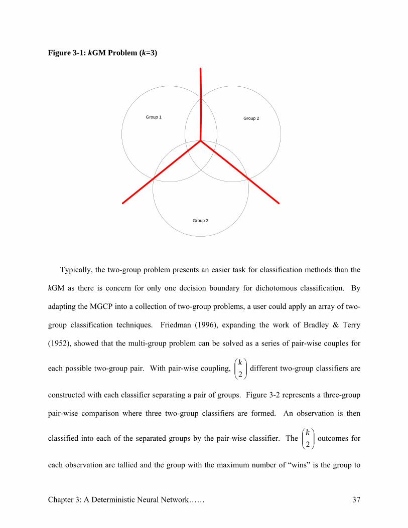
The k-group method (kGM) is the traditional approach to addressing the MGCP. With the
kGM, one classifier is developed from a multi-group data set that assigns an observation into one
of k mutually exclusive groups. The classifier attempts to establish boundaries that separate the
underlying population data. A data point of unknown origin then uses these boundaries as group
classification regions when applied to the problem. Figure 3-1 represents a k=3 group problem
where the kGM has developed decision boundaries. The kGM approach has been employed
extensively in traditional statistical classification research. Unfortunately, this approach is
computationally complex and lacks the flexibility and simplicity of other approaches (Hastie &
Tisbshiran, 1998).
Chapter 3: A Deterministic Neural Network…… 37
Figure 3-1: kGM Problem (k=3)
Group 1 Group 2
Group 3
Typically, the two-group problem presents an easier task for classification methods than the
kGM as there is concern for only one decision boundary for dichotomous classification. By
adapting the MGCP into a collection of two-group problems, a user could apply an array of two-
group classification techniques. Friedman (1996), expanding the work of Bradley & Terry
(1952), showed that the multi-group problem can be solved as a series of pair-wise couples for
each possible two-group pair. With pair-wise coupling, ⎟⎟⎠
⎞⎜⎜⎝
⎛2k
different two-group classifiers are
constructed with each classifier separating a pair of groups. Figure 3-2 represents a three-group
pair-wise comparison where three two-group classifiers are formed. An observation is then
classified into each of the separated groups by the pair-wise classifier. The ⎟⎟⎠
⎞⎜⎜⎝
⎛2k
outcomes for
each observation are tallied and the group with the maximum number of “wins” is the group to

Chapter 3: A Deterministic Neural Network…… 38
which the observation is classified. This pair-wise or “all-against-all” (AAA) approach is a very
intuitive approach to solving the multi-group problem. However, it is computationally expensive
as it requires the creation of ⎟⎟⎠
⎞⎜⎜⎝
⎛2k
classifiers. Therefore, the problem complexity grows along
with the number of groups.
Figure 3-2: ⎟⎟⎠
⎞⎜⎜⎝
⎛2k
Pair-wise Classifiers (k=3)
Group 1 Group 2
Group 3
Group 1
Group 2
Group 3
Classifier (a) Classifier (b)
Classifier (c)

Chapter 3: A Deterministic Neural Network…… 39
Another attempt at reducing the multi-group problem to a series of two-group classification
problems is the “one-against-all” (OAA) approach. In this approach, k different two-group
classifiers, each one trained to distinguish the examples in a single group from the examples in
all remaining groups combined, are developed with each classifier separating a pair of groups,
see Figure 3-3. Each of the k classifiers assigns an output value for an observation that ranges
from zero to one where values close to zero represent membership to the single group and values
close to one represent membership to “all remaining groups”.
In an effort to assess the level of membership to the single group, a classification score
ranging from zero to one is created for each output value. The score is a measure of the distance
from the output value to a value of one based on the separation (or cut-off point) between the two
groups (e.g., an output value close to zero generates a classification score close to one). If the
cut-off point between the two groups occurs at the midpoint in the output range [0,1], the
classification score is simply the difference between one and the classifier output value.
However, when the cut-off point occurs elsewhere in the output range, a weighted distance
measure must be used to generate the classification score. Section 4.2 presents a technique for
generating weighted distance measures. In either case, the single group with the largest
classification score is chosen as the group to which to classify the observation.

Chapter 3: A Deterministic Neural Network…… 40
Figure 3-3: k One-Against-All Classifiers (k=3)
Group 1
CombinedGroup 2&3
Group 2
CombinedGroup 1&3
Group 3
CombinedGroup 1&2
Classifier (a) Classifier (b)
Classifier (c)
Several recent articles suggested AAA is superior to OAA by finding that AAA can be
implemented to calibrate more quickly and test as quickly as the OAA approach (Allwein et al.,
2000 and Hsu & Lin, 2002). However, Rifkin & Klautau (2004) argue against AAA superiority,
as they feel it is not appropriate to simply compare “wins” among pairs and ignore the fact that a
winning margin might be rather small. They find group selection by largest classification score
to be a more appropriate measure for comparison. In their research, they found that the OAA
approach is not superior to the AAA approach, but rather it will perform just as well as AAA.
In most cases, there is no way to know a priori which approach will have more success on a
validation set. With this in mind, Rifkin & Klautau (2004) contend that the OAA approach

Chapter 3: A Deterministic Neural Network…… 41
should be selected over the AAA approach for its overall simplicity, group selection by largest
classification score, and requiring less classification models when the number of groups exceeds
three.
3. CLASSIFICATION METHODS
The aim of a MGCP is to generate a classification rule from a collected data sample
consisting of a set of n observations from k groups. This sample, widely referred to as a
“training sample”, consists of n observations where n1 are known to belong to group 1, n2 are
known to belong to group 2, etc., and n1 + n2 …. + nk = n. This training sample is analyzed to
determine a classification rule applicable to new observations whose true group memberships are
not known.
Unfortunately, there is no classification method that is superior to all others in every
application. Breiman (1994) found that the best classification method changes from one data
context to another. Thus, researchers attempt to devise methods that perform well across a wide
range of classification problems and data sets. In this research, we utilize two common
classification methods which have shown to be effective over a wide range of problems: the
Mahalanobis Distance Measure (MDM) technique that minimizes the probability of
misclassification through distance (Mahalanobis, 1948), and the Backpropagation Neural
Network, which is a universal approximator (Hornik, 1989).
3.1 Mahalanobis Distance Measure
The MDM technique (Mahalanobis, 1948) was established to classify a new observation of
unknown origin into the group it is closest to based on the multivariate distance measure from
the observation to the mean vector for each group (known as the group centroid).

Chapter 3: A Deterministic Neural Network…… 42
More precisely, if we let Dik represent the multivariate distance from observation i to the
centroid of group k, we can calculate the distance as:
)()'( 1kikiik XXCXXD −−= − (1)
where each observation Xi is described by an instance of the vector of independent variables
(i.e., Xi = (Xi1, Xi2,…,Xip)), kX represents the centroid for group k, and C represents the
pooled sample covariance matrix. We allocate Xi to the group for which Dik has the smallest
value (Manly, 1994). It can be shown that the MDM technique is equivalent to Fisher’s Linear
Discriminant Function (Fisher, 1936 and Fisher, 1938), which stands as the benchmark statistical
classifier.
The MDM technique is based on the assumption of multivariate normality among the
independent variables and equal covariance matrices across groups. Under this condition, it
provides “optimal” classification results as it minimizes the probability of misclassification.
However, even when these conditions are violated, the MDM approach can still serve as a
heuristic or classification rate benchmark. In any event, the simplicity, generality, and
intuitiveness of the MDM approach make it a very appealing technique to use on classification
problems (Markham & Ragsdale, 1995).
3.2 Neural Networks
NNs provide another way of generating classifiers for the MGCP. NNs are function
approximation tools that learn the relationship between independent and dependent variables.
However, unlike most statistical techniques for the classification problem, NNs are inherently

Chapter 3: A Deterministic Neural Network…… 43
non-parametric, making no distributional assumptions about the data presented for learning, and
are inherently non-linear, giving them much accuracy when modeling complex data (Smith &
Gupta, 2000).
The primary objective of a NN classifier is to accurately predict group membership of new
data (i.e., data not present in the training sample) whose group membership is not known.
Typically, training data presented to a NN are randomly partitioned into two samples: one for
calibrating (or adjusting the weights in) the NN model and one for periodically testing the
accuracy of the NN during the calibration process.
A NN is composed of a number of layers of nodes linked together by weighted connections.
The nodes serve as computational units that receive inputs and process them into outputs. The
connections determine the information flow between nodes and can be unidirectional, where
information flows only forwards or only backwards, or bidirectional, where information can flow
forwards and backwards (Fausett, 1994).
Figure 3-4 depicts a two-group (k=2) multi-layered feed-forward neural network (MFNN)
where weighted arcs are directed from nodes in an input layer of predictor variables to those in
an intermediate or hidden layer, and then to an output layer.
The back-propagation (BP) algorithm is a widely accepted method used to train MFNN
(Archer & Wang 1993). Wong et al (1997) found approximately 95% of reported business
applications employed the BP algorithm. When training a NN with the BP algorithm, each input
node receives an input value from each of the p independent variables associated with a
calibration sample observation and broadcasts this signal to each of the hidden layer nodes. Each
hidden node then computes its activation (a functional response to the inputs) and sends its signal
to each output node. Each output unit computes its activation to produce the response for the net

Chapter 3: A Deterministic Neural Network…… 44
for the observation in question. The BP algorithm uses supervised learning, meaning that
examples of input (independent) and output (dependent) values of known origin for each of the k
groups are provided to the NN.
Errors are calculated as the difference between the known output and the NN response.
These errors are propagated back through the network and drive the process of updating the
weights between the layers to improve predictive accuracy. In simple terms, NNs “learn” as the
weights are adjusted in this manner. Training begins with random weights that are adjusted
iteratively as calibration observations are presented to the NN. Training continues with the
objective of error minimization until stopping criteria are satisfied (Burke, 1991).
Figure 3-4: Multi-Layered Feed-Forward Neural Network
I1
Ij
Ip
H1
Hj
Hg
O1
O2
Input Units
Hidden Units
Output Units
V1j
V1g
Vj1
Vjj
Vjg
Vpg
Vpj
Vp1
W11
W12
Wj1
Wj2
Wg1
Wg2
V11
To keep a NN from overfitting the calibration data, testing data are periodically presented to
the network to assess the generalizability of the model under construction. The Concurrent

Chapter 3: A Deterministic Neural Network…… 45
Descent Method (CDM) (Hoptroff & Bramson, 1991) is widely used to determine the number of
times the calibration data should be presented to achieve the best performance in terms of
generalization. Using the CDM, the NN is trained for an arbitrarily large number of replications,
with pauses at predetermined intervals. During each pause, the NN weights are saved and tested
for predictive accuracy using the testing data. The average deviation of the predicted group to
the known group for each observation in the testing sample is then calculated and replications
continue (Markham & Ragsdale, 1995). The calibration process stops when the average
deviation on the testing data worsens (or increases). The NN model with the best performance
on the testing data is then selected for classification purposes (Klimasauskas, 2005).
Once a final NN is selected, new input observations of unknown origin may be presented to
the network for classification. Typically, the NN will produce k response values, one for each of
the k groups for each new observation presented. As with the MDM classification technique,
these responses could be interpreted as representing measures of group membership, when
compared to the known k-group output vector, where the smaller (closer to zero) the value
associated with a particular group, the greater the likelihood of the observation belonging to that
group. Thus, the new observation is classified into the group corresponding to the NN output
node producing the smallest response. This resembles a form of the kGM applying MDM. Since
NNs are capable of approximating any measurable function to any degree of accuracy, they
should be able to perform at least as well as the linear MDM technique on non-normal data
(Hornick, et al., 1989).
In Chapter 2, we pointed out several potential weaknesses with a two-group (k=2) NN model
that may arise when training data are randomly partitioned into groups for testing and
calibration. These same potential weaknesses exist for the MGCP. First, the randomly assigned

Chapter 3: A Deterministic Neural Network…… 46
calibration data may not be a good representation of the population from which it was drawn,
potentially leading to a sample-specific model. Second, the testing data may not accurately
assess the generalization ability of a model if they are not chosen wisely. These weaknesses,
individually or together, may adversely affect predictive accuracy and lead to a non-
generalizable NN model. In both cases, the weaknesses arise because of problems with data
partitioning and not from the model building process.
4. DETERMINISTIC NEURAL NETWORK DATA PARTITIONING
4.1 NNDP
In Chapter 2, we introduced a technique to deterministically partition two-group neural
network training data in an effort to improve classification results and combat the potential
shortcomings of random data selection. The Neural Network Data Partitioning (NNDP) heuristic
establishes a technique to “wisely” select testing and calibration samples from training data for a
two-group NN. NNDP is based on MDM from each observation presented for training to its
own group centroid and its opposite group centroid.
To review, a predetermined number of observations having the smallest distances to their
opposite group centroid are selected from the training data as the testing sample. These
observations are the most likely to fall in the region where the groups overlap and be the most
difficult to classify correctly. We focus on this region because this is where the NN’s
classification performance is most critical. Deterministically selecting testing data in this
manner avoids the undesirable situation where none of the testing data fall in the overlap region,
which might occur with random data partitioning (e.g., if the randomly selected testing data
happen to fall tightly around the group centroids).

Chapter 3: A Deterministic Neural Network…… 47
The remaining training data that are not assigned to the testing sample represent the
calibration sample. The calibration sample constitutes values with the largest distances to the
opposite group’s centroid and therefore are most dissimilar to its opposite group and most
representative of their own group. In Chapter 2 we tested the NNDP heuristic on two different
real-world data sets and showed that NNs which applied this heuristic for data pre-processing
outperformed, on average, both a traditional statistical measure (MDM) and a NN built using
randomly partitioned calibration and testing samples. Thus, we concluded that the NNDP
heuristic decreased overfitting and increased predictive accuracy for the two small data sets.
4.2 kNNDP
The next logical step is to expand the notion of deterministic partitioning of NN training data
to MGCPs. We introduce a multi-group heuristic based on the NNDP heuristic to improve
classification results and address the potential shortcomings of random data selection on small
multi-group data sets. We refer to this heuristic as the kNNDP heuristic.
The kNNDP heuristic requires several steps. First we perform a random hold-out sampling
from data presented for classification. This hold-out or validation sample will ultimately be used
to validate the accuracy of our heuristic. The remaining data, known as training data, will be
used to construct our classification model.
Next, the training data, composed of k different groups, are paired in k different ways based
on the OAA approach. We selected the OAA approach over the AAA approach because it treats
MGCPs as a series of k two-group comparisons and uses classification scores for comparability.
As stated previously, the OAA approach requires the creation of k different two-group
classifiers, each one trained to distinguish the examples in a single group from the examples in

Chapter 3: A Deterministic Neural Network…… 48
all remaining groups. In addition, we did not select the kGM as the approach to which we would
apply deterministic partitioning. The kGM approach presents a significant challenge for
determining minimum distance to an opposite group centroid as two or more opposite group
centroids are present. We experimented with an array of distance values for partitioning, but
could not define a deterministic selection rule that proved effective. Thus, based on the success
NNDP exhibited on two-group classification problems, we selected a technique that reduces a
MGCP to a series of two-group classification problems.
For the next step, the NNDP heuristic is applied to each of the k different two-group
problems resulting in deterministically partitioned calibration and testing samples for each of the
k pairs. This data are then used to build k different NN classifiers (one for each OAA pair)
through the application of a MFNN trained with BP.
Finally, we apply each of the k classifiers to every observation of our validation sample and
make classifications based on the OAA approach. That is, a comparable classification score
must be generated for each validation observation in order to choose the most appropriate group.
To accomplish this, our NN models are built with a single output node which provides a network
response value between zero and one. Each validation record would therefore be represented by
k values between zero and one where output values close to zero represent membership to the
single group and an output near one represents membership to “all remaining groups”. Recall
that a classification score ranging between zero and one is developed for each of the k output
values as a measure of group membership for the single groups. The generation of a
classification score requires identifying a cut-off point or threshold (T) between zero and one to
select the appropriate distance measure calculation. Klimasauskas et al. (2005) suggest a unique

Chapter 3: A Deterministic Neural Network…… 49
method for creating cut-off points between groups, which they refer to as the K-S (Kolmogorov-
Smirnov) threshold, which has shown to be highly effective in NN applications.
The K-S threshold is based on how well the NN classifier has separated the two target
groups. Cumulative histograms with 40 non-overlapping intervals formed from the predicted
outputs of the calibration data for the two target groups are overlaid. The K-S threshold is the
leading-edge value of the interval containing the greatest distance between corresponding NN
output values in the two histograms. The greatest distance measure is referred to as the K-S
statistic. Figure 3-5 is an example of a K-S threshold generation measured over nine intervals
(rather than 40) for illustrative purposes. If a model were to output random values, the
cumulative histograms would both be fairly linear and the K-S statistic would have a value close
to zero. If the model were perfect, the Group 0 value would accumulate to one immediately and
the Group 1 value would ascend from a value of zero to a value of one at the neural network
output value of one (Klimasauskas et al., 2005).
Figure 3-5: K-S Threshold Generation
K-S Statistic
Cumulative Histogram for Single Group (0)
Cumulative Histogram for All Remaining Groups (1)
K-S Threshold (T)
Perc
enta
ge o
f Cal
ibra
tion
Dat
a
Neural Network Predicted Output Values0 1
100%

Chapter 3: A Deterministic Neural Network…… 50
The K-S statistic provides a natural split between groups and an associated threshold by
which an observation can be classified (e.g., a NN output below the K-S statistic would be
classified to Group 0 (single group) and a value above the K-S threshold (T) would be classified
to Group 1 (all remaining groups)). Using the K-S threshold as the cut-off point, we can
generate classification scores where each NN output is valued based on its distance from this
threshold.
The classification scores are developed as follows:
1. If an observation’s NN output equals T, the classification score equals .5
2. If an observation’s NN output is less than T, the classification score equals:
.5 + .5*((T - NN Output)/T))
3. If an observation’s NN output is greater than T, the classification score equals:
.5 - .5*((NN Output - T)/(1 - T))
So, rather than performing a simple comparison of NN outputs, we generate k classification
scores for each validation record. We then select the largest classification score and identify its
associated group as the group to which we will classify that observation.
5. EXPERIMENTAL DESIGN
In an effort to evaluate the classification ability of our kNNDP heuristic, we tested four different
methods for solving the MGCP:
• RP-MDM – applying the MDM technique with randomly partitioned training data
• RPNN-kGM – applying NNs with randomly partitioned training data for the kGM
approach

Chapter 3: A Deterministic Neural Network…… 51
• RPNN-OAA – applying NNs with randomly partitioned training data for the OAA
approach
• kNNDP – applying NNs with kNNDP as the training data pre-processing heuristic
for the OAA approach
The predictive accuracy of each technique will be assessed against three different data sets.
For this research, we have chosen two real-world data sets and one simulated data set in an effort
to provide different classification challenges for the four classification methods. The three were
selected for their completeness (no missing values), variety, and size. They were extracted from
UCSB database (Newman et al., 1998).
The first real-world data set is the 1,473 record contraceptive method choice data which are a
subset of the 1987 National Indonesia Contraceptive Prevalence Survey. This three-group data
set is used to predict the current contraceptive method (none, long-term, and short-term) used by
non-pregnant married women based on their demographic and socio-economic characteristics.
Nine different attributes were collected by researchers for each participant: (1) age, (2)
educational level, (3) husband’s educational level, (4) number of children ever born, (5) religion,
(6) employed, (7) husband’s occupation, (8) standard-of-living index, and (9) level of media
exposure. This data set is comprised of 629 reporting no-use, 333 reporting long-term use, and
511 reporting short-term use and was previously used in (Lim et al., 1999).
The second real-world data set represents teaching assistant evaluation data that marks the
evaluation of teaching performance as low, medium, or high. Data were gathered over three
regular semesters and two summer sessions of 96 teaching assistants at the Statistics Department
of the University of Wisconsin, Madison. The researchers collected information on each
teaching assistant over five select variables: (1) whether or not the teaching assistant’s first

Chapter 3: A Deterministic Neural Network…… 52
language was English, (2) the course instructor, (3) the course number, (4) regular semester or
summer session, and (5) class size. This data set contains scores for 32 low, 32 medium, and 32
high scores and was previously used in (Loh & Shih, 1997 and Lim et al., 1999).
The simulated data set is the balance scale weight and distance data originally appearing in
Sielger (1976). This data set was generated to model the results of psychological experiments.
Each data record is classified to one of three groups having the balanced scale tip to the right,
left, or balanced. The variables that comprise each record are left weight, left distance, right
weight, and right distance. Group assignment is found as the greater of (left distance * left
weight) and (right distance * right weight). If they are equal, then the assignment is balanced.
This data set contains 625 records where 49 are balanced, 288 are left, and 288 are right. The
data has been previously used in (Klahr, 1978, Langley, 1987, Newell, 1990, McClelland, 1988,
and Shultz, 1994).
A summary of all three data sets can be found in Figure 3-6.
Figure 3-6: Summary of Data Sets
Balanced Contraceptive TeachingScale Prevalence Assistant
Number of Observations 625 1,473 96
-Group 1 49 629 32-Group 2 288 333 32-Group 3 288 511 32
Number of Variables 4 9 5
For experimental testing purposes, each data set undergoes a random hold-out sampling
which results in two data samples, one for training and one for validation of the model. The
training data will be used with each of the four solution methodologies for model building

Chapter 3: A Deterministic Neural Network…… 53
purposes. While the NN driven techniques partition the training data into two samples
(calibration and testing) for model building purposes, the MDM technique will use all the
training data with no intermediate model testing. The validation data represent “new”
observations to be presented to each of the four modeling techniques for classification; allowing
the predictive accuracy of the various techniques to be assessed on observations that had no role
in developing the respective classification functions. Thus, the validation data provides a good
test for how well the classification techniques might perform when used on observations
encountered in the future whose true group memberships are unknown.
To assess the effect of training sample size on the various classification techniques, we
required the training and validation sample sizes to be nearly equivalent but still allow for even
partitioning of training data. Figure 3-7 represents the randomly split data sizes in the study by
data set and sample. Based on our assessment of small data set size, only the teaching assistant
data set can be considered a small data set as the total number of training data falls below its
adequate sample size threshold. In this case, the threshold was 90 (6*5 predictor variables*3
groups) and the training data size was 48 observations.
Figure 3-7: Summary of Data Assignments
Balanced Contraceptive TeachingScale Prevalence Assistant
Training Data 314 760 48
Calibration Sample 157 380 24 Testing Sample 157 380 24
Validation Data 311 713 48

Chapter 3: A Deterministic Neural Network…… 54
All observations assigned to the training sample are used in the MDM technique for model
building. All NN techniques use the same training sample as the MDM technique, but split the
training data into testing and calibration samples in a 50/50 split, with an equal assignment of
each group in each sample based on their assigned pre-processing technique. The kNNDP
technique selects the half of each group that is closest to its opposite group centroid as the testing
data. The remaining observations are assigned as calibration data. The random partitioning
techniques randomly assign half of each group to the testing and calibration data. We generated
30 different models for each method and data set combination.
A Microsoft EXCEL add-in was used to generate the MDM classification results as well as
the distances used for data pre-processing for the kNNDP heuristic. The NNs used in this study
were developed using NeuralWorks™ Predict® (Klimasauskas, 2005). The standard back-
propagation configuration was used. The NNs used sigmoidal activation functions for nodes in
the hidden and output layers. All remaining settings for Predict were default settings.
6. RESULTS
6.1 Balanced Scale Weight and Distance Data
Figure 3-8 lists the percentage of correctly classified observations in the validation data for
each of the 30 replications performed on the balance scale weight and distance data. We found
that the average classification rate for the NN that employed the kNNDP heuristic was 91.37%.
This value exceeded the RPNN-kGM, RPNN-OAA, and RP-MDM techniques which had
classification rates of 90.79%, 90.46%, and 74.97% respectively. We also found that the kNNDP
approach produced the largest number of highest classification rates (“wins”) among these

Chapter 3: A Deterministic Neural Network…… 55
techniques. Although it did not always produce the highest percentage, it posted significantly
more “wins” than the other three methods.
It should also be noted that, on average, the kNNDP technique was shown to be significantly
different than the other three other techniques. We also found the RPNN-kGM and RPNN-OAA
techniques were not significantly different. So, in this case, applying the OAA approach to a NN
employing randomly partitioned training data does not produce a classifier that outperforms a
NN with randomly partitioned training data for the k-group method. However, as noted
previously, an application of kNNDP to a NN outperforms all other methods tested on this data.
6.2 Contraceptive Prevalence Survey Data
Figure 3-9 lists the percentage of correctly classified observations in the validation data for
each of the 30 replications performed on the contraceptive prevalence survey data. We found
that the average classification rate for the NN that employed the kNNDP heuristic was 56.19%.
This value exceeded the RPNN-kGM, RPNN-OAA, and RP-MDM techniques which had
classification rates of 53.19%, 53.79%, and 50.15% respectively. We also found that the kNNDP
approach produced the largest number of highest classification rates (“wins”) among techniques.
Although it did not always produce the highest percentage, it posted significantly more “wins”
than the other three methods.
It should also be noted that, on average, the kNNDP technique was shown to be significantly
different than the other three other techniques. Additionally, the RPNN-kGM and RPNN-OAA
techniques were not significantly different. So, in this case, applying the OAA approach to a NN
employing randomly partitioned training data does not produce a classifier that outperforms a

Chapter 3: A Deterministic Neural Network…… 56
NN with randomly partitioned training data for the k-group method. However, once again we
found that an application of kNNDP to a NN outperforms all other methods tested on these data.
6.3 Teaching Assistant Evaluation Data
Figure 3-10 lists the percentage of correctly classified observations in the validation data for
each of the 30 replications performed on the teaching assistant evaluation data. Recall that
earlier we determined this data set to be small, so therefore the potential problems of neural
network classification may be heightened. However, we found that the average classification
rate for the NN that employed the kNNDP heuristic to be 70.35% which exceeded the RPNN-
kGM, RPNN-OAA, and RP-MDM techniques. Each had classification rates of 62.50%, 65.56%,
and 67.43% respectively. We also found that the kNNDP approach produced the largest number
of highest classification rates (“wins”) among techniques. Although it did not always produce
the highest percentage, it posted significantly more “wins” than the other three methods.
It should also be noted that, on average, kNNDP technique was shown to be significantly
different than the other three other techniques. Additionally, the RPNN-kGM and RPNN-OAA
techniques were found to be significantly different. So, in this case, applying the OAA approach
to a NN employing randomly partitioned training data did produce a classifier that outperforms a
NN with randomly partitioned training data for the k-group method. However, in this last data
set, we again found that an application of kNNDP to a NN outperforms all other methods tested
on this data and that a wisely partitioned NN is appropriate for small data set usage.

Chapter 3: A Deterministic Neural Network…… 57
7. IMPLICATIONS AND CONCLUSIONS
7.1 Implications
Several important implications arise from this research. First, by expanding the use of the
NNDP heuristic to MGCPs, we see that the developed kNNDP heuristic holds considerable
promise in eliminating the innate negative effects that random data partitioning can have on
building a generalizable NN. While further testing is necessary, it appears that the kNNDP
technique will perform at least as well as traditional statistical techniques and standard NNs that
use a random calibration and testing data assignment. This is particularly important for small
data sets for, as we saw in our study, the most significant impact on results was with the small
teaching assistant evaluation data.
Second, our results show the kNNDP technique which applies OAA produces improvements
over an application of OAA to randomly partitioned NN training data. This is important as it
shows the impact of the heuristic is more than simple data manipulation. This result is important
as, potentially, a deterministic data partitioning approach, similar to kNNDP, could be applied to
other classification techniques.
Finally, many commercial NN software packages do not provide the capability for anything
other than random partitioning of the training data. This appears to be a serious weakness that
software vendors should address.
7.2 Conclusions
The kNNDP heuristic has been introduced that combines the data classification properties of
a traditional statistical technique (MDM) with a NN to create classification models that are less
prone to overfitting. By deterministically partitioning training data into calibration and testing

Chapter 3: A Deterministic Neural Network…… 58
samples, undesirable effects of random data partitioning are shown to be mitigated.
Computational testing shows the kNNDP heuristic proved superior to other widely accepted
methods for MGCPs over an array of varying data sizes. Perhaps most significantly, application
of the kNNDP heuristic may help increase the applicability of NNs for classification problems
with small training samples. Thus, the kNNDP heursitic holds considerable promise and warrants
further investigation.

Chapter 3: A Deterministic Neural Network…… 59
Figure 3-8: Percentage of Correctly Classified Observations for Balanced Scale Weight and Distance Data
Run RP-MDM RPNN-kGM RPNN-OAA k NNDP1 70.74% 92.28% 90.35% 92.93%2 74.60 89.39 90.03 90.353 69.13 91.32 90.68 91.324 77.17 93.25 90.68 92.285 77.17 90.78 89.71 89.396 77.17 90.35 90.68 90.037 67.85 85.53 88.75 89.718 76.85 92.28 90.03 90.359 79.10 90.03 90.68 90.3510 77.81 90.35 90.68 90.0311 78.14 93.57 91.96 93.5712 73.63 87.46 91.64 92.2813 69.77 89.71 90.35 90.0314 73.63 90.68 91.96 90.0315 82.96 91.64 90.68 92.6016 78.78 89.39 90.03 91.6417 76.85 94.21 90.35 94.5318 73.63 90.03 88.75 91.6419 74.60 88.42 91.96 92.6020 81.03 93.25 86.50 93.8921 73.95 91.64 89.39 91.3222 70.74 92.28 91.00 93.2523 74.60 88.42 90.68 89.7124 69.13 91.32 88.75 90.3525 77.17 92.93 90.03 93.2526 78.46 91.32 91.64 90.6827 73.31 90.03 91.00 89.7128 73.95 91.32 91.00 90.6829 73.95 88.42 91.96 90.6830 73.31 91.96 91.96 91.96
Average 74.97% 90.79% 90.46% 91.37%
Wins 0 9 10 15
Tests for Differences in the Average Rate of ClassificationComparison t-value*RPNN-k GM vs k NNDP 1.989 *RPNN-OAA vs k NNDP 2.582 *RP-MDM vs k NNDP 25.288 *RPNN-k GM vs RPNN-OAA 0.745
* t-value significant at α=.05

Chapter 3: A Deterministic Neural Network…… 60
Figure 3-9: Percentage of Correctly Classified Observations for Contraceptive Prevalence Suvery Data
Run RP-MDM RPNN-kGM RPNN-OAA k NNDP1 50.35% 56.10% 54.14% 59.89%2 49.23 53.44 52.17 54.983 50.21 54.00 55.82 59.474 50.07 50.07 53.02 57.785 51.47 54.56 55.54 55.966 51.33 55.12 55.82 57.787 49.23 48.53 55.12 57.088 51.75 54.98 57.92 59.899 51.89 54.14 55.12 54.9810 51.61 53.30 57.50 57.2211 47.83 48.67 51.61 56.8012 48.11 52.73 48.95 54.0013 48.81 52.03 51.89 55.4014 49.93 54.42 53.72 55.6815 48.67 48.67 50.49 56.9416 51.75 54.56 54.14 56.2417 49.51 55.54 57.08 51.1918 50.35 52.03 52.73 52.4519 48.81 53.02 52.31 54.0020 49.79 56.52 53.86 54.1421 50.35 49.93 54.52 54.4222 49.23 50.21 52.17 55.1223 50.21 54.14 56.52 58.7724 50.07 51.89 51.89 56.1025 51.47 54.89 53.72 54.2826 48.25 55.40 53.86 59.1927 53.72 55.82 52.17 58.3528 51.05 54.00 54.56 55.1229 50.21 54.70 51.47 58.0630 49.09 52.31 54.00 54.28
Average 50.15% 53.19% 53.79% 56.19%
Wins 0 2 5 23
Tests for Differences in the Average Rate of ClassificationComparison t-valueRPNN-k GM vs k NNDP 5.500 *RPNN-OAA vs k NNDP 4.846 *RP-MDM vs k NNDP 14.371 *RPNN-k GM vs RPNN-OAA 1.337
* t-value significant at α=.05

Chapter 3: A Deterministic Neural Network…… 61
Figure 3-10: Percentage of Correctly Classified Observations for Teaching Assistant Evaluation Data
Run RP-MDM RPNN-kGM RPNN-OAA k NNDP1 72.92% 60.42% 66.67% 77.08%2 77.08 72.92 68.75 77.083 64.58 66.67 70.83 70.834 72.92 70.83 75.00 79.175 66.67 64.58 62.50 64.586 66.67 50.00 64.58 68.757 70.83 66.67 72.92 68.758 62.50 66.67 62.50 64.589 77.08 68.75 75.00 75.00
10 66.67 60.42 56.25 66.6711 66.67 64.58 56.25 72.9212 62.50 66.67 70.83 66.6713 64.58 66.67 75.00 72.9214 68.75 72.92 72.92 72.9215 70.83 56.25 58.33 83.3316 64.58 52.08 50.00 56.2517 62.50 45.83 54.17 60.4218 54.17 64.58 58.33 68.7519 72.92 54.17 62.50 72.9220 68.75 72.92 72.92 66.6721 68.75 54.17 64.58 70.8322 70.83 62.50 66.67 70.8323 54.17 52.08 54.17 58.3324 77.08 75.00 77.08 77.0825 64.58 56.25 66.67 66.6726 60.42 66.67 64.58 70.8327 68.75 39.58 58.33 66.6728 66.67 58.33 66.67 70.8329 62.50 77.08 70.83 70.8330 75.00 68.75 70.83 81.25
Average 67.43% 62.50% 65.56% 70.35%
Wins 10 4 8 18
Tests for Differences in the Average Rate of ClassificationComparison t-valueRPNN-k GM vs k NNDP 5.105 *RPNN-OAA vs k NNDP 4.037 *RP-MDM vs k NNDP 3.213 *RPNN-k GM vs RPNN-OAA 2.606 *
* t-value significant at α=.05

Chapter 3: A Deterministic Neural Network…… 62
References: Allwein, E. L., Schapire, R.E., & Singer, Y. (2000). Reducing multiclass to binary: a unifying
approach for margin classifiers. Journal of Machine Learning Research (1), 113-141. Archer, N.P. & Wang, S. (1993). Application of the back propagation neural network algorithm
with monotonicity constraints for two-group classification problems. Decision Sciences 24(1), 60-75.
Bradley, R. & Terry, M. (1952). The rank analysis of incomplete block designs, the method of
paired comparisons. Biometrika (39), 324-345. Breiman, L. (1994). Discussion of the paper by Ripley. Journal of Royal Statistical Society,
56(3), 445. Burke, L.L. (1991). Introduction to artificial neural systems for pattern recognition, Computers
and Operations Research 18(2), 211-220. Crammer, K. & Singer, Y. (2002). On the learnability and design of output codes for multiclass
problems. Machine Learning 47(2), 201-233. Delmaster, R., & Hancock, M. (2001). Data mining explained, Boston: Digital Press. Dietterich, T.G. & Bakiri, G. (1995). Solving multiclass problems via error-correcting output
codes. Journal of Artificial Intelligence Research (2), 263-186. Fausett, L. (1994). Fundamentals of neural networks: architectures, algorithms, and applications
(Prentice Hall, Upper Saddle River). Fisher, R. A. (1936). The use of multiple measurements in taxonomic problems. Annals of
Eugenics (7), 179-188. Fisher, R. A. (1938). The statistical utilization of multiple measurements. Annals of Eugenics
(8), 376-386. Friedman, J. Another approach to polychotomous classification. Technical Report, Stanford
University. Furnkranz, J. (2002). Round robin classification. Journal of Machine Learning Research
(2),721-747. Gochet, W., Stam, A., Srinivasan, V., & Chen, S. (1997). Multigroup discrimination analysis
using linear programming. Operations Research 45(2), 213-225. Hastie, T. & Tibshirani, R. (1998). Classification by pairwise coupling. The Annals of Statistics
26(2), 451-471.

Chapter 3: A Deterministic Neural Network…… 63
Hoptroff, R., Bramson, M., & Hall, T. (1991). Forecasting economic turning points with neural
nets, IEEE INNS International Joint Conference of Neural Networks, Seattle, 347-352. Hornick, K., Stinchcombe, M., & White, H. (1989). Multilayer feedforward networks are
universal approximators, Neural Networks (2), 359-366. Hsu, C. & Lin, C. (2002). A comparison of methods for multi-class support vector machines.
IEEE Transactions on Neural Networks (13), 415-425. Klahr, D., & Siegler, R.S. (1978). The representation of children's knowledge. In H. W. Reese
& L. P. Lipsitt (Eds.), Advances in Child Development and Behavior, pp. 61-116. New York: Academic Press
Klimasauskas, C.C., Guiver, J.P., and Pelton, G. (2005). NeuralWorks Predict (NeuralWare, Inc.,
Pittsburg). Konstam, A. (1994). N-group classification using genetic algorithms, Symposium on Applied
Computing, Proceedings of the 1994 ACM symposium on Applied computing, Phoenix, ACM Press 212-216.
Lam, K. F, Choo, E. U., & Moy, J. W. (1996). Minimizing deviations from the group mean: A
new linear programming approach for the two-group classification problem. European Journal of Operational Research (88), 358-367.
Langley,P. (1987). A general theory of discrimination learning. In D. Klahr, P. Langley, & R.
Neches (Eds.), Production System Models of Learning and Development, pp. 99-161. Cambridge, MA: MIT Press
Lee, Y., Lin, Y., & Wahba, G. (2001). Multicategory support vector machines. Technical Report
1043, Department of Statistics, University of Wisconsin. Lim, T.-S., Loh, W.Y. & Shih, Y.-S. (1999). A comparison of prediction accuracy, complexity,
and training time of thirty-three old and new classification algorithms. Machine Learning.Forthcoming.
Loh, W.-Y. & Shih, Y.S. (1997). Split selection methods for classification trees, Statistica Sinica
(7), 815-840. Mahalanobis, P.C. (1948). Historical note on the D2-statistic. Sanhkya (9), 237. Manly, B. (1994). Multivariate statistical methods: a primer (Chapman and Hall, London). Markham, I.S. & Ragsdale, C.T. (1995). Combining neural networks and statistical predictions
to solve the classification problem in discriminant analysis, Decision Sciences (26), 229-242.
Chapter 3: A Deterministic Neural Network…… 64
McClelland, J.L. (1988). Parallel distributed processing: implications for cognition and development. Technical Report AIP-47, Department of Psychology, Carnegie-Mellon University.
Moller, M (1992). Supervised learning on large redundant training sets. Neural Networks for
Signal Processing [1992] II., Proceedings of the 1992 IEEE-SP Workshop, 79-89. Newell, A. (1990). Unified theories of cognition. Cambridge, MA: Harvard University Press Newman, D.J. & Hettich, S. & Blake, C.L. & Merz, C.J. (1998). UCI Repository of machine
learning databases [http://www.ics.uci.edu/~mlearn/MLRepository.html]. Irvine, CA: University of California, Department of Information and Computer Science.
Ostermark, R. (1999). A fuzzy neural network algorithm for multigroup classification, Fuzzy
Sets and Systems (105), 113-122. Patel, N., Shmueli, G., & Bruce, P. (2005). Data mining in Excel: lecture notes and cases,
Resampling Statistics, Inc., Arlington, VA (pg 16). Plutowski, M. & White, H. (1993). Selecting concise training sets from clean data. IEEE
Transaction on Neural Networks 4(2), 305-318. Rifkin, R. & Klautau, A. (2004). In defense of one-vs-all classification. Journal of Machine
Learning Research (5), 101-141. Shultz, T., Mareschal, D., & Schmidt, W. (1994). Modeling cognitive development on balance
scale phenomena. Machine Learning (16), 59-88. Siegler, R. S. (1976). Three aspects of cognitive development. Cognitive Psychology (8), 481-
520. Smith, K.A. & Gupta, J.N.D. (2000). Neural networks in business: techniques and applications
for the operations researcher, Computers and Operations Research (27), 1023-1044. Subramanian, V., Hung, M., & Hu, M. (1993). An experimental evaluation of neural networks
for classification. Computers and Operational Research 20 (7), 769-782. Weston, J. & Watkins, C. (1998). Multi-class support vector machines. Technical Report CSD-
TR-98-04, Royal Holloway, University of London, Department of Computer Science. Wong, B.K., Bodnovich, T.A, & Selvi, Y. (1997). Neural network applications in business: a
review and analysis of the literature (1988-1995). Decision Support Systems (19), 301-320.

Chapter 4: Big Bang Discriminant Analysis….. 65
Chapter 4
Bing Bang Discriminant Analysis: Exploring the Edges of the Neural Network Training Data Universe

Chapter 4: Big Bang Discriminant Analysis….. 66
1. INTRODUCTION
In Chapter 2 we focused on the development of a deterministic Neural Network Data
Partitioning (NNDP) heuristic for two-group training data. The success that the heuristic
exhibited on real-world data is of practical importance as ultimately the strength of any
classification technique is how well it performs under experimental conditions with real-world
data. However, much of the current research in discriminant analysis employs simulated data.
Simulated data allow researchers much flexibility for testing as large amounts of data can be
generated quickly by individual researchers for specific classification problems. Although the
advantages of simulating data are desirable, there are pitfalls with the most obvious being that
simulated data generally do not resemble real-world data (Hooker, 1996). This begs the
question: How well do simulated neural network training data approximate real-world data?
In this chapter, we address this question by examining the position of neural network training
data with respect to their location within group convex polyhedrons. We present a training data
positioning algorithm, apply it to several common real-world and simulated data sets, and
compare the general positions. In addition, we test the applicability of NNDP to two-group
simulated data through its application to several simulated data sets and examine its
classification accuracy against several commonly used classification techniques. Next, following
the success NNDP exhibited on real-world data, we examine whether developing a pre-
processing technique that transforms the position of simulated data to positions that resemble
real-world data enhances the performance of NNDP and improves classification accuracy. Last,
we present our findings and discuss implications.

Chapter 4: Big Bang Discriminant Analysis….. 67
2. BACKGROUND
As stated previously, the objective of the two-group classification problem in discriminant
analysis is to identify a function that accurately distinguishes observations as originating from
one of two mutually exclusive groups. Researchers have developed numerous approaches for the
two-group classification problem, but the problem still remains a major challenge in many forms
of decision making. Mangiameli & West (1999) confirm this by stating that no classification
model is best for all data sets. They suggest building models that give good classification results
across a wide range of problems.
A common practice among researchers is to compare the classification accuracy of NNs
against other classification techniques. Boritz et al. (1995), Coates & Fant (1992), Etheridge &
Sriram (1996), Fanning & Cogger (1994), Pendley et al. (1998), Tam & Kiang (1992), Markham
& Ragsdale (1995) are among many who followed this path. A general consensus among
researchers is that NNs do create classifiers that fit training data well.
Rumelhart et al. (1986) supports this finding by stating that appropriately designed NNs have
consistently been shown to generate good separation in training data sets. However, NNs
provided mixed results when classifying new observations of unknown origin (Lehar & Weaver,
1987 and Archer & Wang, 1993). So, the generalizability of a neural network to new data of
unknown origin is heavily dependent on the proper use of training data. We will show this also
requires an understanding of the data’s position in space.
Zobel et al. (2006) recently developed a method for identifying a new observation’s position
relative to the convex polyhedrons of each training data group. The authors established a
boundary generation algorithm to determine class membership by locating the relative position

Chapter 4: Big Bang Discriminant Analysis….. 68
of a new observation with respect to the existing class boundaries. Their algorithm identifies a
point as being located within the shape, on the boundary, or outside the shape.
By applying a similar algorithm to neural network training data for the two group problem,
we can establish the position of the training data for each group as interior to or on the boundary
of their specific group convex polyhedron. In this way, we establish the position of data to be
used for classification and assess the selection of test samples for NNDP.
3. TRAINING DATA POSITION ALGORITHM
3.1 Methodology
The identification of an observation’s position with respect to its own group convex
polyhedron is established through convex combinations. A convex combination is any point on
the line segment joining two points xa and xb of the form λxa + (1-λ)xb where 0 ≤ λ ≤ 1 (Bazaraa
et al., 2004). A set X in Rn is called a convex set if the convex combination formed by any pair
of points in X lies entirely within X. The intersection of all convex sets within X is known as a
convex hull. A convex polyhedron is the shape formed by the exterior faces of the convex hull.
The convex polyhedron surrounds a bounded volume of interior space (Weisstein, 2002).
The collection of all training data for a particular group defines a convex polyhedron for that
group. Each training data observation exists on the interior or the boundary of the convex
polyhedron associated with the group to which it belongs. An interior point is contained
entirely within the form while a boundary point can occur as a vertex (or extreme point) or as a
perimeter point (or a point on a polygonal face).
Any interior observation can be written as a convex combination of two or more boundary
points of the polyhedron. Any perimeter observation between a pair of vertices can be written as

Chapter 4: Big Bang Discriminant Analysis….. 69
a convex combination of the vertices. However, an observation that is a vertex cannot be formed
as a convex combination of any other points within the polyhedron. For simplicity, we will refer
to points as either interior or boundary.
So, given a set of observations of the form ),...,,( 21 ipiii xxxx = , the following linear
programming problem identifies an observation xk as an interior or boundary point.
(BB) Max α (1) s.t.
)( xxxx ki
ii −+=∑ αλ (2)
1=∑
iiλ (3)
0=kλ (4) 0≥iλ (5)
That is, we attempt to find the largest distance multiplier,α , in (1) that, when starting at the
group centroid x and moving in a direction towards xk, results in a point that is a convex
combination of observations from the data set excluding xk. The possible solutions for α are:
• If (BB) has a feasible solution with α =1, then xk is a perimeter point,
• If (BB) has a feasible solution with α > 1, then xk is an interior point,
• If (BB) is infeasible, then xk is a vertex.
It should be noted that for this application, a feasible solution with α < 1 will not be present as
the training data are composed entirely of interior and boundary points. This result stems from
only the training data points used in the formulation of the group centroid being tested.
However, it is possible for points not used in the generation of the group centroid to fall outside

Chapter 4: Big Bang Discriminant Analysis….. 70
of the convex polyhedron. In such cases, feasible solutions with α < 1 would indicate exterior
points.
3.2 Application
To evaluate the performance of the data positioning algorithm, we assessed the data position of
several real-world data sets using (BB). These sets include:
Boston Housing Data
This two group data set includes 14 attributes for 506 records. It was collected by the US Census
Service concerning housing in the area of Boston Massachusetts. The data were originally
published by Harrison & Rubinfeld (1978).
Hepatitis Domain Data
This two group data set includes 20 attributes for 155 records for hepatitis diagnosis and whether
the subject lived or passed away. The data were originally published by Diaconis & Efron
(1983).
Texas Bank Data
This two group data sample consists of Texas banks that failed in the period 1985-1987. It
consists of 162 records with 19 attributes. This data set appeared numerous times in the
literature, notably in Tam & Kiang (1992).

Chapter 4: Big Bang Discriminant Analysis….. 71
Credit Approval Data
This two group data set includes 15 attributes for 653 records for credit card applications and
whether the subjects were approved or denied credit. The data were originally published by
Quinlan (1987).
Wisconsin Breast Cancer Data
This two group data set was obtained from the University of Wisconsin Hospitals, Madison from
Dr. William H. Wolberg and consists of 699 records with 9 attributes. The data were originally
published by Mangasarian &Wolberg (1990).
Moody’s Industrial Data
This two group data sample consists of 4 attributes with 46 records and represents annual
financial data from Moody’s Industrial Manuals. These data were obtained from Johnson &
Wichern (1998).
Results from applying the data positioning algorithm to each data set can be seen in Figure 4-1.
Figure 4-1: Real-World Data Position
Total Number of Number of Number of Data Sets Observations Attributes Boundary Points Interior PointsBoston Housing 506 14 506 (100%) 0 (0%)Hepatitis Domain 155 20 155 (100%) 0 (0%)Texas Bank 162 19 162 (100%) 0 (0%)Credit Approval 653 15 653 (100%) 0 (0%)Wisconsin Breast Cancer 699 9 694 (99%) 5 (1%)Moody's Industrial 46 4 40 (87%) 6 (13%)

Chapter 4: Big Bang Discriminant Analysis….. 72
As the data reveal, the majority (4 out of 6) of data sets contain no interior points and thus are
composed entirely of boundary points (perimeter points and vertices) positioned on group
specific convex polyhedrons. The sets that do contain interior points, the Breast Cancer and
Moody’s data sets, contain only 1% and 13% interior points each. The results suggest that real-
world data is dominated by boundary points.
Next, we wanted to evaluate several simulated data sets from the literature using (BB). The
data sets include:
Multivariate Normal Distribution with Identity Variance/Covariance Matrices
Samples are drawn from two multivariate normal populations with three attributes. The first is
distributed N(μ1,I) and the second is distributed N(μ2,I), where:
μ1 = [6.5, 6.5, 6.5] and μ2 = [5.5, 5.5, 5.5],
respectively (Lam et al., 1996).
Bivariate Normal Distribution with Unequal Variance/Covariance Matrices
Samples are drawn from the bivariate normal distribution with unequal variance covariance
matrices. They were drawn from:
⎟⎟⎠
⎞⎜⎜⎝
⎛=
55
1μ , ⎟⎟⎠
⎞⎜⎜⎝
⎛=
515
2μ , ⎟⎟⎠
⎞⎜⎜⎝
⎛=∑
255.75.725
1 , ⎟⎟⎠
⎞⎜⎜⎝
⎛=∑
255.225.22225
2
(Patuwo et al., 1993).

Chapter 4: Big Bang Discriminant Analysis….. 73
Multivariate Normal Distribution with Outlier Observations
Samples are drawn from two multivariate normal populations with three variates. The first is
distributed N(μ1,I) and the second is distributed N(μ2,I), where:
μ1 = [10.0, 10.0, 10.0] and μ2 = [11.5, 11.5, 11.5],
with equal covariance matrices for both. To contaminate the population, approximately 10% of
the observations generated were then replaced by outlier observations. The outlier observations
for the first group were generated using the transformation:
• For group 1, b i0 = μi0 + 3 + δ0,
• For group 2, b i1 = μi1 - 3 - δ1,
where δ0 and δ1 were drawn from the Beta distribution with parameters α = 5, β = 1.5 and α =
1.5, β = 5, respectively (Stam & Ragsdale, 1992).
Beta Distribution
Samples are drawn from two Beta distributions with five variables.
11 )1()),(/1()( −− −= qp xxqpBxf where B(p,q) = ∫ −− −1
0
11 )1( dxxx qp
Beta Data Sets Group 1 Group 2 Variable 1 p=1.4 and q=3.0 p=3.0 and q=1.5 Variable 2 p=2.5 and q=4.0 p=4.0 and q=2.5 Variable 3 p=3.0 and q=5.0 p=3.0 and q=5.0 Variable 4 p=2.0 and q=3.0 p=3.0 and q=2.0 Variable 5 p=4.0 and q=5.0 p=5.0 and q=4.0
(Sueyoshi et al., 2006).

Chapter 4: Big Bang Discriminant Analysis….. 74
For each method, 200 data records were simulated (100 for each group) over 10 replications
and the position results averaged. Figure 4-2 reports the position findings.
Figure 4-2: Simulated Data Position
Total Number of Number of Number of Data Sets Observations Attributes Boundary Points Interior PointsLam et al.,1996 200 3 43 (22%) 157 (78%)Patuwo et al.,1993 200 2 21 (11%) 179 (89%)Stam & Ragsdale,1992 200 3 51 (26%) 149 (74%)Sueyoshi et al.,2006 200 5 145 (73%) 55 (27%)
The results show that the typical data position of several commonly used simulated data sets
do not a reflect the boundary-centric characteristics of the commonly used real-world data sets
we tested. Rather, the composition is starkly different. The real-world data were almost entirely
boundary points, while the simulated data present as primarily interior points. Interestingly, the
two data sets used in Chapter 2, the Texas Bankruptcy and Moody’s, are shown to be markedly
different from the simulated data we tested in this chapter. So, to fully examine the impact of the
NNDP heuristic, we need to apply NNDP to training data with more interior data points (similar
to the simulated data) than the two sets used to originally evaluate the heuristic.
4. SIMULATED DATA PERFORMANCE TEST
In Chapter 2, we evaluated the performance of data sets against three classification methods:
MDM, NN and NNDP.

Chapter 4: Big Bang Discriminant Analysis….. 75
4.1 Mahalanobis Distance Measure
The MDM technique attempts to classify a new observation of unknown origin into one of
two groups. Developed by Mahalanobis (1948), the MDM approach calculates the multivariate
distance of a new observation of unknown group origin to the centroid of each of the two groups.
The observation is classified as belonging to the group to which it has the minimum distance.
Under certain conditions (i.e., multivariate normality of the independent variables in each
group and equal covariance matrices across groups) the MDM approach provides “optimal”
classification results in that it minimizes the probability of misclassification. Even when these
conditions are violated, the MDM approach can still be used as a heuristic (although other
techniques might be more appropriate). In any event, the simplicity, generality, and intuitiveness
of the MDM approach make it a very appealing technique to use on classification problems
(Markham & Ragsdale, 1995).
4.2 Neural Networks
NNs are function approximation tools that learn the relationship between independent and
dependent variables. However, unlike most statistical techniques for the classification problem,
NNs are inherently non-parametric and make no distributional assumptions about the data being
modeled (Smith & Gupta, 2000).
A NN is composed of a number of layers of nodes linked together by weighted connections.
The nodes serve as computational units that receive inputs and process them into outputs. The
connections determine the information flow between nodes and can be unidirectional, where
information flows only forwards or only backwards, or bidirectional, where information can flow
forwards and backwards (Fausett, 1994).

Chapter 4: Big Bang Discriminant Analysis….. 76
A multi-layered feed-forward neural network (MFNN) is a very common application where
weighted arcs are directed from nodes in an input layer to those in an intermediate or hidden
layer, and then to an output layer.
The back-propagation (BP) algorithm is the most widely used neural network training
algorithm used in business applications. When training a NN with the BP algorithm, each node
in the input layer receives a value from an independent variable associated with a calibration
sample observation and broadcasts this signal to each of the hidden layer nodes. Each hidden
node then computes its activation (a functional response to the inputs) and sends its signal to
each output node. Each output unit computes its activation to produce the response for the net
for the observation in question. The BP algorithm uses supervised learning, meaning that
examples of input (independent) and output (dependent) values from known origin for each of
the two groups are provided to the NN.
Typically, the known output value for each example is provided. Errors are calculated as the
difference between the known output and the NN response. These errors are propagated back
through the network and drive the process of updating the weights between the layers to improve
predictive accuracy. In simple terms, NNs “learn” as the weights are adjusted in this manner.
Training begins with random weights that are adjusted iteratively as calibration observations are
presented to the NN. Training continues with the objective of error minimization until stopping
criteria are satisfied (Burke, 1991).
To keep a NN from overfitting the calibration data, testing data are periodically presented to
the network to assess the generalizability of the model under construction. The concurrent
descent method (CDM) (Hoptroff et al., 1991) is widely used to determine the number of times
the calibration data should be presented to achieve the best performance in terms of

Chapter 4: Big Bang Discriminant Analysis….. 77
generalization. Using the CDM, the NN is trained for an arbitrarily large number of replications,
with pauses at predetermined intervals. During each pause, the NN weights are saved and tested
for predictive accuracy using the testing sample. The average deviation of the predicted group to
the known group for each observation in the testing sample is then calculated and replications
continue (Markham & Ragsdale, 1995). The calibration process stops when the average
deviation on the testing data worsens (or increases). The NN model with the best performance
on the testing data is then selected for classification purposes (Klimasauskas et al., 1989).
Once a final NN is selected, new input observations may be presented to the network for
classification. For the two-group case, the NNs used in this study produce two response values;
one response for each of the two groups for each new observation presented. As with the MDM
classification technique, these responses could be interpreted as representing measures of group
membership, when compared to the known two-group output vector, where the smaller (closer to
zero) the value associated with a particular group, the greater the likelihood of the observation
belonging to that group. Thus, a new observation is classified into the group corresponding to
the NN output node producing the smallest response.
Since NNs are capable of approximating any measurable function to any degree of accuracy
they should be able to perform at least as well as the linear MDM technique on non-normal data
(Hornick et al., 1989). However, several potential weaknesses may arise when data presented for
NN model building is randomly partitioned into the samples needed for testing and calibration.
First, the randomly assigned calibration sample may not be a good representation of the
population from which it was drawn, potentially leading to a sample-specific NN model.
Second, the randomly assigned testing sample may not accurately assess the generalizability of a
model if it is not chosen wisely. These weaknesses, individually or together, may adversely

Chapter 4: Big Bang Discriminant Analysis….. 78
affect predictive accuracy and lead to a non-generalizable NN model. In both cases, the
weaknesses arise because of problems with data partitioning and not from the model building
process.
4.3 NNDP Heuristic
The Neural Network Data Partitioning (NNDP) heuristic utilizes MDM to select testing and
calibration samples in the two-group classification problem. MDM is used to calculate distances
for each training sample observation to both group centroids. These two distance values
represent: (1) the distance from each observation to its own group centroid and (2) the distance
from each observation to the opposite group's centroid.
We select a predetermined number of observations having the smallest distances to the
opposite group's centroid as the testing sample. These observations are those most apt to fall in
the region where the groups overlap. Observations in the overlap region are the most difficult to
classify correctly. Hence, this area is precisely where the network’s classification performance is
most critical. Selecting the testing data in this manner avoids the undesirable situation where no
testing data falls in the overlap region, which might occur with random data partitioning (e.g., if
the randomly selected testing data happens to fall tightly around the group centroids).
The training observations not assigned to the testing sample constitute the calibration sample.
Thus, the calibration sample consists of observations with the largest distances to the opposite
group’s centroid and therefore are most dissimilar to the opposite group and most representative
of their own group.
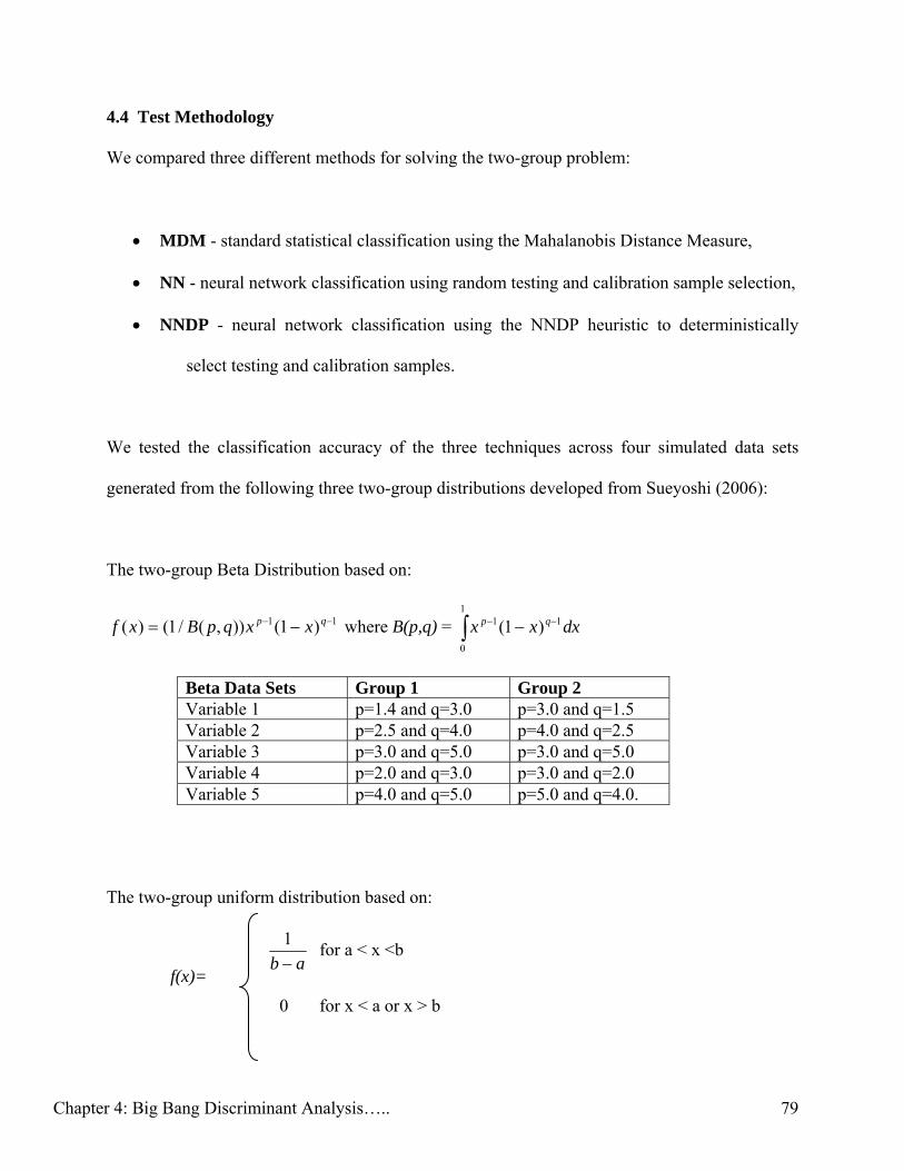
Chapter 4: Big Bang Discriminant Analysis….. 79
4.4 Test Methodology
We compared three different methods for solving the two-group problem:
• MDM - standard statistical classification using the Mahalanobis Distance Measure,
• NN - neural network classification using random testing and calibration sample selection,
• NNDP - neural network classification using the NNDP heuristic to deterministically
select testing and calibration samples.
We tested the classification accuracy of the three techniques across four simulated data sets
generated from the following three two-group distributions developed from Sueyoshi (2006):
The two-group Beta Distribution based on:
11 )1()),(/1()( −− −= qp xxqpBxf where B(p,q) = ∫ −− −1
0
11 )1( dxxx qp
Beta Data Sets Group 1 Group 2 Variable 1 p=1.4 and q=3.0 p=3.0 and q=1.5 Variable 2 p=2.5 and q=4.0 p=4.0 and q=2.5 Variable 3 p=3.0 and q=5.0 p=3.0 and q=5.0 Variable 4 p=2.0 and q=3.0 p=3.0 and q=2.0 Variable 5 p=4.0 and q=5.0 p=5.0 and q=4.0.
The two-group uniform distribution based on:
ab −
1 for a < x <b
0 for x < a or x > b
f(x)=

Chapter 4: Big Bang Discriminant Analysis….. 80
Uniform Data Sets Group 1 Group 2 Variable 1 U(3,10) U(0.1,7) Variable 2 U(3,10) U(0.1,7) Variable 3 U(2,10) U(0.1,8) Variable 4 U(0.1,8) U(2,10) Variable 5 U(0.1,8) U(2,10).
The two-group Normal Distribution based on:
)2
)(exp(2
1)( 2
2
σμ
πσ−
−=xxf
Normal Data Sets Group 1 Group 2 Variable 1 N(15,3) N(11,3) Variable 2 N(20,5) N(13,5) Variable 3 N(30,8) N(20,8) Variable 4 N(13,5) N(20,5) Variable 5 N(11,3) N(15,3).
We generated 150 observations for each of the two groups using the distributions described
above. Four data sets were then generated as follows:
• Data Set 1: Observations drawn from the two-group Beta Distribution
• Data Set 2: Observations drawn from the two-group Uniform Distribution
• Data Set 3: A ratio of observations drawn from the two-group Beta Distribution to
observations drawn from the two-group Uniform Distribution
• Data Set 4: A ratio of observations drawn from the two-group Uniform Distribution to
observations drawn from the two-group Normal Distribution.

Chapter 4: Big Bang Discriminant Analysis….. 81
For experimental testing purposes, each data set undergoes a random hold-out sampling
which results in two data samples, one for validation and one for training the model. Thus, for
each group, 50 observations were assigned to validation, while the remaining 100 observations
were allocated to training. The training data will be used with each of the three solution
methodologies for model building purposes. While the NN driven techniques partition the
training data into two samples (calibration and testing) for model building purposes, the MDM
technique will use all the training data with no intermediate model testing. The validation data
represent “new” observations to be presented to each of the four modeling techniques for
classification; allowing the predictive accuracy of the various techniques to be assessed on
observations that had no role in developing the respective classification functions. Thus, the
validation data provide a good test for how well the classification techniques might perform
when used on observations encountered in the future whose true group memberships are
unknown.
As stated previously, all observations assigned to the training sample are used in the MDM
technique for model building. All NN techniques use the same training sample as the MDM
technique, but split the training data into testing and calibration samples in a 50/50 split, with an
equal assignment of each group in each sample based on their assigned pre-processing technique.
We generated 30 different models for each technique.
A Microsoft EXCEL add-in was used to generate the MDM classification results as well as
the distances used for data pre-processing for the NNDP heuristic. The NNs used in this study
were developed using NeuralWorks™ Predict® (Klimasauskas, 2005). The standard back-
propagation configuration was used. The NNs used sigmoidal activation functions for nodes in
the hidden and output layers. All remaining settings for Predict were default settings.

Chapter 4: Big Bang Discriminant Analysis….. 82
4.5 Results
The results of the application are seen in Figure 4-3.
Figure 4-3: Simulated Data Classification Rate Accuracy
Data MDM NN NNDPData Set 1 88.6% 85.7% 87.2%Data Set 2 91.6% 86.3% 87.8%Data Set 3 81.0% 91.0% 91.9%Data Set 4 82.8% 85.2% 86.8%
We found that the NNDP heuristic outperformed the default randomly partitioned neural
network, on average, in each data set but did not prove significantly different. Also, the NNDP
does not outperform MDM in every data set as it did on the data sets in Chapter 2.
Recall from Chapter 2 that the NNDP heuristic outperformed the default NN and MDM
when the training data was all or almost all boundary data. We decided to examine if shifting all
interior data, when available, to positions on the boundary in a direction starting at the group
centroid, and then applying the NNDP heuristic, provides a similar result. By projecting points
in this manner, we are reinforcing the boundary of the convex polyhedron with additional data
points. This is important as ultimately the boundaries of the group polyhedrons define the
classifier. In addition, we hope to increase the difficulty of classification of observations that are
to be selected as testing data with NNDP. Our intention is to increase the number of
observations that occur in or near the overlap region. By doing so, we create observations that
have been shown to be the most difficult to classify. This is important for observations from one
group that might have been selected as testing data based on distance to their opposite group
centroid and appeared exclusively in their own convex polyhedron. Such an observation would
not present a difficult challenge for a classifier in its original position; however when it is
Chapter 4: Big Bang Discriminant Analysis….. 83
projected to the boundary, the difficulty is magnified. The remaining observations that are not
selected for the testing sample will again be assigned to the calibration sample. The projected
calibration sample provides the model with observations that are easy to classify, but more
difficult than a calibration sample from the unprojected data. Our hope is that the projected data,
when deterministically partitioned by NNDP, will provide a more generalizable model than the
three techniques tested previously. Therefore, we intend to show that when data are shifted to all
boundary positions, an application of the NNDP heuristic outperforms MDM, NN, and NNDP.
5. BOUNDARY NNDP HEURISTIC
The Boundary NNDP heuristic utilizes the fact that the training sample observations form a
convex polyhedron with each observation located on the boundary or contained within the shape
of each group. Figure 4-4(a) demonstrates the generation of a convex polyhedron for a single
group.
The first step is to calculate multivariate distances from each training observation to its own
group centroid using MDM. We select a small arbitrary amount of values farthest from their
group centroid and remove them from the hull. We refer to these values as outliers. Steuer
(1986) suggested that using all such extreme values may not be necessary in constructing such
forms because of lack of contribution to the model. A new convex polyhedron composed of the
remaining training observations is generated using all original group observations to create the
centroid. Figure 4-4(b) demonstrates the removal of outliers and generation of a new
polyhedron.

Chapter 4: Big Bang Discriminant Analysis….. 84
Next, we project all interior points and newly severed exterior points for each group to the
boundary region of each new group convex hull. To accomplish this task, we must employ
(BB). For this application, possible solutions are:
• If (BB) has a feasible solution with α =1, then xk is a perimeter point and no position
change is required,
• If (BB) has a feasible solution with α > 1, then xk is an interior point and the solution for
)( xxx k −+α represents a projected position on the boundary of the polyhedron for the
point,
• If (BB) has a feasible solution with α < 1, then xk is an exterior point and the solution for
)( xxx k −+α represents a projected position on the boundary of the polyhedron for the
point,
• If (BB) is infeasible, then xk is a vertex and no position change is required.
Figure 4-4(c) demonstrates the projection of data to the boundary of the convex polyhedron.
This results in the creation of two boundary only polyhedrons. Figure 4-4(d) demonstrates the
generation of a boundary only convex polyhedron for a single group.
Finally, the NNDP heuristic is introduced to our newly formed boundary only training
samples and a neural network is developed. The intention of this effort is to replicate the success
NNDP had on training data heavily composed of boundary data in Chapter 2.

Chapter 4: Big Bang Discriminant Analysis….. 85
Figure 4-4: Boundary NNDP Convex Polyhedron
`
`
`
`
`
`
`
` `
`
`
`
`
`
`
`
Group Centroid
(a) Convex Polyhedron – All Training Observations
`
`
`
`
`
`
`
` `
`
`
`
`
`
`
`
Group Centroid
(b) Convex Polyhedron – Removing Outliers
`
`
`
`
`
`
`
` `
`
`
`
`
`
`
`
Group Centroid
(c) Convex Polyhedron – Interior/Exterior Point Projection
`
``
`
` `
`
`
`
`
Group Centroid
`
`
`
` `
`
(d) Convex Polyhedron – Converted Boundary Data

Chapter 4: Big Bang Discriminant Analysis….. 86
6. EXPERIMENTAL DESIGN
In an effort to evaluate the effectiveness of our Boundary NNDP heuristic, we intend to compare
its performance against three other classification techniques for the two-group problem:
• MDM - standard statistical classification using the Mahalanobis Distance Measure,
• NN - neural network classification using random testing and calibration sample selection,
• NNDP - neural network classification using the NNDP heuristic to deterministically
select testing and calibration samples.
• Boundary NNDP – neural network classification that applies the NNDP heuristic to
deterministically select testing and calibration samples for data that has been
projected to the convex polyhedron boundary
We follow the same testing methodology used previously. In addition, when applying the
Boundary NNDP heuristic we will hold out 10% of the training observations as outliers. This is
a conservative estimate based on Hample et al.’s (1986) assertion that between 1% and 10% of
the data points in a typical data set contain outliers. The following results are based on the
generation of 30 different models for each technique.

Chapter 4: Big Bang Discriminant Analysis….. 87
7. RESULTS
7.1 Data Set 1: Beta Distribution
Figure 4-5 lists the percentage of correctly classified observations in the validation data for
each of the 30 replications performed on the Beta distribution data. We found that the average
classification rate for the NN that employed the Boundary NNDP heuristic was 88.9%. This
value exceeded the MDM, default NN with random data partitioning, and a NN employing the
NNDP heuristic. The actual classification rate results were of 88.0%, 85.2%, and 86.2%
respectively. We also found that the Boundary NNDP approach produced the largest number of
highest classification rates (“wins”) among techniques. Although it did not always produce the
highest percentage, it posted significantly more “wins” than the other three methods.
It should also be noted that, on average, the Boundary NNDP technique was shown to be
significantly different than the other three other techniques. We also found the NN with random
data partitioning and a NN employing the NNDP heuristic were not significantly different,
although NNDP did perform better on average.
7.2 Data Set 2: Uniform Distribution
Figure 4-6 lists the percentage of correctly classified observations in the validation data for
each of the 30 replications performed on the Uniform distribution data. We found that the
average classification rate for the NN that employed the Boundary NNDP heuristic was 90.2%.
This value exceeded the classification rates for MDM (89.7%), default NN with random data
partitioning (87.0%), and a NN employing the NNDP heuristic (88.0%). We also found that the
Boundary NNDP approach produced the largest number of highest classification rates (“wins”)

Chapter 4: Big Bang Discriminant Analysis….. 88
among techniques. Although it did not always produce the highest percentage, it posted
significantly more “wins” than the other three methods.
It should also be noted that, on average, the Boundary NNDP technique was shown to be
significantly different than the NN with random data partitioning and a NN employing the
NNDP heuristic. We also found the NN with random data partitioning and a NN employing the
NNDP heuristic were not significantly different, although NNDP did perform better on average.
7.3 Data Set 3: Beta Distribution-Uniform Distribution Ratio
Figure 4-7 lists the percentage of correctly classified observations in the validation data for
each of the 30 replications performed on the Beta-Uniform ratio data. We found that the average
classification rate for the NN that employed the Boundary NNDP heuristic was 93.2%. This
value exceeded the MDM, default NN with random data partitioning, and a NN employing the
NNDP heuristic. The actual classification rate results were of 81.0%, 90.8%, and 91.3%
respectively. We also found that the Boundary NNDP approach produced the largest number of
highest classification rates (“wins”) among techniques. Although it did not always produce the
highest percentage, it posted significantly more “wins” than the other three methods.
It should also be noted that, on average, the Boundary NNDP technique was shown to be
significantly different than the other three other techniques. We also found the NN with random
data partitioning and a NN employing the NNDP heuristic were not significantly different,
although NNDP did perform better on average.

Chapter 4: Big Bang Discriminant Analysis….. 89
7.4 Data Set 4: Uniform Distribution -Normal Distribution Ratio
Figure 4-8 lists the percentage of correctly classified observations in the validation data for
each of the 30 replications performed on the Uniform-Normal ratio data. We found that the
average classification rate for the NN that employed the Boundary NNDP heuristic was 93.5%.
This value exceeded the MDM, default NN with random data partitioning, and a NN employing
the NNDP heuristic. The actual classification rate results were of 86.9%, 90.1%, and 90.4%
respectively. We also found that the Boundary NNDP approach produced the largest number of
highest classification rates (“wins”) among techniques. Although it did not always produce the
highest percentage, it posted significantly more “wins” than the other three methods.
It should also be noted that, on average, the Boundary NNDP technique was shown to be
significantly different than the other three other techniques. We also found the NN with random
data partitioning and a NN employing the NNDP heuristic were not significantly different,
although NNDP did perform better on average.
8. IMPLICATIONS AND CONCLUSIONS
8.1 Implications
Several important implications stem from this research. First, through a direct comparison of
the relative data position of real-world and simulated data sets, we found that the typical position
of points is markedly different. Real-world data tended to be boundary dominant, while the
simulated data tended to be interior dominant. Second, by projecting interior points and outlier
exterior points to the convex polyhedron boundary, we form a generalizable neural network
model that outperforms several well known techniques as well as an effective heuristic
established in Chapter 2. While further testing is necessary, it appears that the Boundary NNDP

Chapter 4: Big Bang Discriminant Analysis….. 90
technique will perform at least as well as traditional statistical techniques, standard NNs that use
a random calibration and testing data assignment, and NNs employing NNDP when addressing
training data sets containing interior points.
Our results show the Boundary NNDP technique produces improvements over our NNDP
heuristic applied to our original un-projected training sample. This is important as it shows the
impact of boundary points on the development of a generalizable model. Ultimately the true
success of a heuristic is how well it performs on real-world data. It is our hope that extending
the Boundary NNDP heuristic to interior point laden real-world data maximizes the application
of NNDP and improves classification accuracy.
Finally, many commercial NN software packages do not provide the capability for anything
other than random partitioning of the training data. This appears to be a serious weakness that
software vendors should address.
8.2 Conclusions
The Boundary NNDP heuristic has been introduced that enhances the effect of the NNDP
heuristic introduced in Chapter 2. Computational testing shows the Boundary NNDP heuristic
performed at least as well, and in most cases superior to other widely accepted methods for the
two-group classification problem. Application of the Boundary NNDP heuristic may help
increase the applicability of NNs for real-world classification problems with a large number of
interior points than we have seen. Thus, the Boundary NNDP heuristic holds considerable
promise and warrants further investigation.

Chapter 4: Big Bang Discriminant Analysis….. 91
Figure 4-5: Percentage of Correctly Classified Observations for Data Set 1
Run MDM NN NNDP Boundary NNDP1 87% 83% 87% 89%2 79 77 79 823 87 89 89 924 93 87 90 935 88 84 87 886 95 90 91 957 91 84 86 918 89 90 89 899 91 89 89 9310 86 84 85 8711 89 83 89 9112 85 87 90 8913 84 84 86 8814 92 85 90 9115 92 92 91 9316 86 85 84 8617 92 92 86 9318 90 90 89 9119 88 87 89 9020 88 85 75 8721 92 86 89 9122 87 87 87 8923 86 73 84 8424 82 78 79 8225 90 86 86 9126 90 91 89 9227 84 83 81 8428 83 75 82 8229 86 85 84 8730 88 85 85 88
Average 88.0% 85.2% 86.2% 88.9%
Wins 13 1 1 23
Tests for Differences in the Average Rate of ClassificationComparison t-valueMDM vs Boundary NNDP 3.119 *NN vs Boundary NNDP 7.868 *NNDP vs Boundary NNDP 6.139 *NN vs NNDP 1.489
* t-value significant at α=.05
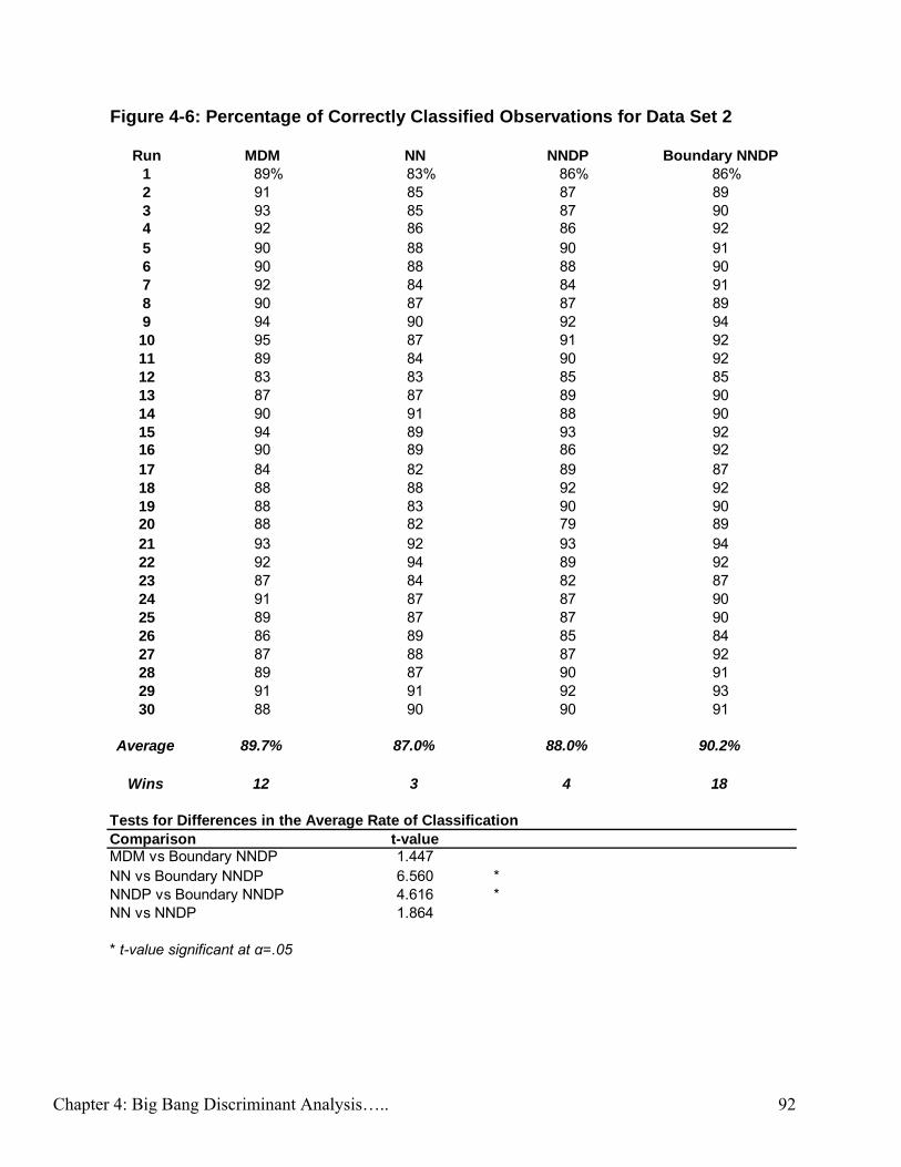
Chapter 4: Big Bang Discriminant Analysis….. 92
Figure 4-6: Percentage of Correctly Classified Observations for Data Set 2
Run MDM NN NNDP Boundary NNDP1 89% 83% 86% 86%2 91 85 87 893 93 85 87 904 92 86 86 925 90 88 90 916 90 88 88 907 92 84 84 918 90 87 87 899 94 90 92 9410 95 87 91 9211 89 84 90 9212 83 83 85 8513 87 87 89 9014 90 91 88 9015 94 89 93 9216 90 89 86 9217 84 82 89 8718 88 88 92 9219 88 83 90 9020 88 82 79 8921 93 92 93 9422 92 94 89 9223 87 84 82 8724 91 87 87 9025 89 87 87 9026 86 89 85 8427 87 88 87 9228 89 87 90 9129 91 91 92 9330 88 90 90 91
Average 89.7% 87.0% 88.0% 90.2%
Wins 12 3 4 18
Tests for Differences in the Average Rate of ClassificationComparison t-valueMDM vs Boundary NNDP 1.447NN vs Boundary NNDP 6.560 *NNDP vs Boundary NNDP 4.616 *NN vs NNDP 1.864
* t-value significant at α=.05
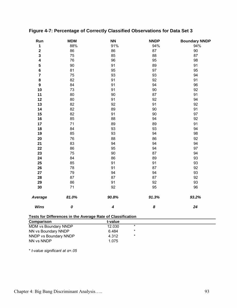
Chapter 4: Big Bang Discriminant Analysis….. 93
Figure 4-7: Percentage of Correctly Classified Observations for Data Set 3
Run MDM NN NNDP Boundary NNDP1 88% 91% 94% 94%2 86 86 87 903 75 85 88 874 76 96 95 985 90 91 89 916 81 95 97 957 75 93 93 948 82 91 92 919 84 91 94 96
10 73 91 90 9211 80 90 87 9112 80 91 92 9413 82 92 91 9214 82 89 90 9115 82 91 90 9716 85 88 94 9217 71 89 89 9118 84 93 93 9419 85 93 94 9820 76 88 86 9221 83 94 94 9422 86 95 94 9723 75 90 87 9424 84 86 89 9325 85 91 91 9326 78 91 87 9227 79 94 94 9328 87 87 87 9229 86 91 92 9330 71 92 95 96
Average 81.0% 90.8% 91.3% 93.2%
Wins 0 4 8 24
Tests for Differences in the Average Rate of ClassificationComparison t-valueMDM vs Boundary NNDP 12.030 *NN vs Boundary NNDP 6.484 *NNDP vs Boundary NNDP 4.312 *NN vs NNDP 1.075
* t-value significant at α=.05

Chapter 4: Big Bang Discriminant Analysis….. 94
Figure 4-8: Percentage of Correctly Classified Observations for Data Set 4
Run MDM NN NNDP Boundary NNDP1 84% 85% 83% 88%2 77 93 95 973 81 81 81 864 83 75 92 915 83 77 81 856 84 89 87 957 74 93 86 928 89 79 80 899 86 92 87 92
10 87 88 96 9511 90 92 90 9312 89 98 96 9713 90 95 93 9514 89 86 94 9515 86 94 92 9316 86 92 88 9517 93 91 89 9318 93 86 88 9119 92 95 93 9520 84 93 95 9621 87 92 97 9822 88 95 88 9123 93 93 93 9524 86 95 93 9625 93 95 89 9726 85 91 92 9427 86 92 91 9128 87 94 95 9729 89 90 91 9630 94 93 92 98
Average 86.9% 90.1% 90.4% 93.5%
Wins 3 8 3 22
Tests for Differences in the Average Rate of ClassificationComparison t-valueMDM vs Boundary NNDP 7.415 *NN vs Boundary NNDP 4.572 *NNDP vs Boundary NNDP 4.996 *NN vs NNDP 0.431
* t-value significant at α=.05

Chapter 4: Big Bang Discriminant Analysis….. 95
REFERENCES Archer, N.P. & Wang, S. (1993). Application of the back propagation neural network algorithm
with monotonicity constraints for two-group classification problems. Decision Sciences 24(1), 60-75.
Bazaraa, M., Jarvis, J., & Sherali, H. (2004). Linear programming and network flows, 3rd edition
(Wiley-Interscience, New York). Boritz, JE, Kennedy, DB, & de Miranda, A. (1995). Predicting corporate failure using a neural
network approach. Intelligent Systems in Accounting, Finance, and Management (4), 95-111.
Burke, L.L. (1991). Introduction to artificial neural systems for pattern recognition, Computers
and Operations Research 18(2), 211-220. Coates, P.K. & Fant, L.F. (1992). A neural network approach to forecasting financial distress.
The Journal of Business Forecasting (3), 8-12. Diaconis, P. & Efron, B. (1983). Computer-Intensive Methods in Statistics. Scientific American,
Volume 248. Etheridge, H & Sriram, R. (1996). A neural network approach to financial distress analysis.
Advances in Accounting Information Systems (4), 201-222. Fanning, K & Cogger, K (1994). A comparative analysis of artificial neural networks using
financial distress prediction. Intelligent Systems in Accounting, Finance, and Management (3), 241-252.
Fausett, L. (1994). Fundamentals of neural networks: architectures, algorithms, and applications
(Prentice Hall, Upper Saddle River). Hample, F.R., Ronchetti, E.M., Rousseeuw, P.J., & Stahel, W.A. (1986). Robust statistics: the
approach based on influence functions (John Wiley, New York). Harrison, D. & Rubinfeld, D.L. (1978). Hedonic prices and the demand for clean air, J. Environ.
Economics & Management (5), 81-102. Hooker, J.N. (1986). Testing Heuristics: We Have It All Wrong, Journal of Heuristics (1), 33-42. Hoptroff, R., Bramson, M., & Hall, T. (1991). Forecasting economic turning points with neural
nets, IEEE INNS International Joint Conference of Neural Networks, Seattle, 347-352.
Hornick, K., Stinchcombe, M., & White, H. (1989). Multilayer feedforward networks are universal approximators, Neural Networks (2), 359-366.

Chapter 4: Big Bang Discriminant Analysis….. 96
Johnson, R.A. & Wichern, D.W. (1998). Applied multivariate statistical analysis (4th edition)
(Prentice Hall, Upper Saddle River). Klimasauskas, C.C., Guiver, J.P., & Pelton, G. (2005). NeuralWorks Predict (NeuralWare, Inc.,
Pittsburg). Lam, K. F, Choo, E. U., & Moy, J. W. (1996). Minimizing deviations from the group mean: A
new linear programming approach for the two-group classification problem. European Journal of Operational Research (88), 358-367.
Lehar, S. & Weaver, J. (1987). A developmental approach to neural network design.
Proceedings of the IEEE First International Conference on Neural Networks. New York. Mahalanobis, P.C. (1948). Historical note on the D2-statistic. Sanhkya 9, 237. Mangasarian, O. L. & Wolberg, W. H. (1990). Cancer diagnosis via linear programming, SIAM
News (23)5, 1 & 18. Mangiameli, P. & West, D. (1999). An improved neural classification network for the two-group
problem, Computers & Operations Research (26), 443-460. Markham, I.S. & Ragsdale, C.T. (1995). Combining neural networks and statistical predictions
to solve the classification problem in discriminant analysis, Decision Sciences (26), 229-242. Patuwo, E., Hu, M.Y., & Hung, M.S. (1993). Two-group classification using neural networks,
Decision Sciences 24(4), 825-845. Pendley, J.A,. Glorfeld, L.W., & Hardgrave, B. (1998). Bankruptcy prediction of financially
distressed firms: an extension of the use of artificial neural networks to evaluate going concern. Advances in Accounting Information Systems. (6), 163-184.
Quinlan, C. (1987). Simplifying decision trees, International Journal of Man-Machine Studies
(27), 221-234. Rumelhart, DE, Hinton, G, & Williams, R. (1986). Learning representation by back-propagation
errors, Nature (323) 9, 533-536. Smith, K.A. & Gupta, J.N.D. (2000). Neural networks in business: techniques and applications
for the operations researcher, Computers and Operations Research (27), 1023-1044. Stam, A. & Ragsdale, C. (1992). On the classification gap in mathematical-programming-based
approaches to the discriminant problem, Naval Research Logistics (39), 545-559. Steuer, R. (1986). Multiple criteria optimization: theory, computation, and application (Wiley,
New York).

Chapter 4: Big Bang Discriminant Analysis….. 97
Sueyoshi, T. (2006). DEA-Discriminant analysis methodological comparison among eight
discriminant analysis approaches, European Journal of Operational Research (169), 247-272. Tam, K.Y. & Kiang, M.Y. (1992). Managerial applications of neural networks: the case of bank
failure prediction, Management Science 38(7), 926-947. Weisstein, E.W., “Convex Polyhedron”, From MathWorld—A Wolfram Web Resource.
http://mathworld.wolfram.com/ConvexPolyhedron.htm. Zobel, C., Cook, D., & Ragsdale, C. (2006). Data driven classification using boundary
observations. Decision Sciences, Forthcoming.

Chapter 5: Conclusions and Future Research 98
Chapter 5
Conclusions and Future Research

Chapter 5: Conclusions and Future Research 99
SUMMARY
The classification of data has become a necessary routine for many businesses. It involves
identifying a function that accurately classifies observations as originating from one of two or
more mutually exclusive groups. For businesses, neural networks have become the most
commonly applied technique for function development.
In this dissertation, we identified and discussed a number of potential problems with typical
random partitioning of neural network training data for the classification problem and introduced
deterministic methods to partitioning that overcame these obstacles and improved classification
accuracy on new validation data. We presented heuristics for both the two-group classification
problem and k-group classification problem and showed that these heuristics produced
generalizable neural network models that were more accurate, on average, than several
commonly used classification techniques.
In addition, we compared several two-group simulated and real-world data sets with respect
to the interior and boundary positions of observations within their groups’ convex polyhedrons.
By projecting the interior points of simulated data to the boundary of their group polyhedrons,
we generated convex shapes similar to real-world data convex polyhedrons. Through an
application of our two-group deterministic partitioning heuristic to the repositioned simulated
data, we produced data classification accuracy that was superior to several commonly used
classification techniques.

Chapter 5: Conclusions and Future Research 100
FUTURE RESEARCH
“Top Hat” Deterministic Neural Network Data Partitioning
In this research we add our deterministic neural network data partitioning heuristics to
existing neural network classification modeling enhancements (e.g., improved networks,
architectures, or stopping rules) in an effort to extend classification accuracy. The heuristics
introduced in this dissertation were tested with default neural networks so we assert that this
research should do no worse than maintain the level of classification accuracy of the modeling
enhancements and more likely will improve classification accuracy.
Big-Bang Data Generation
In this dissertation we introduced a heuristic to project interior points to the boundary of their
group convex polyhedrons. This effort helped to reinforce the boundary and increase the number
of potential observations in the overlap region. In this research, we suggest generating boundary
points in a similar manner but maintaining the original position of the interior points as well.
This would increase the number of training observations, a potential benefit for very small data
sets, and not only reinforce the boundary, but provide interior coverage for calibration samples as
well. Our hope is that by increasing the number of observations, while maintaining the integrity
of the original group convex polyhedrons, we could enhance the generalizability of a neural
network model.

Chapter 5: Conclusions and Future Research 101
CONCLUSIONS
This dissertation presents an interesting and often neglected area of neural network research,
training data partitioning. In this research, we introduce methods to deterministically partition
neural network training data for the classification problem which counter the typical random
partitioning methodology. We show by example that deterministically partitioning training data
into calibration and testing samples, based on the application of a statistical distance measure,
produces neural network models that exhibit superior classification accuracy over several widely
accepted classification techniques. Furthermore, we show that the relative position of two-group
real-world and simulated data sets are starkly different. We develop a heuristic to transform the
position of simulated data observations into positions similar to typical real-world data. We
show by example that applying our two-group deterministic data partitioning heuristic to the
transformed data produces neural network models that are more accurate, on average, than
several well known classification techniques.
`

References 102
REFERENCES
Abad, P.L. & Banks, W.J. (1993). New LP based heuristics for the classification problem, European Journal of Operational Research (67), 88-100.
Allwein, E. L., Schapire, R.E., & Singer, Y. (2000). Reducing multiclass to binary: a
unifying approach for margin classifiers. Journal of Machine Learning Research (1), 113-141.
Archer, N.P & Wang, S. (1993). Application of the back propagation neural network algorithm with monotonicity constraints for two-group classification problems, Decision Sciences 24(1), 60-75.
Bazaraa, M., Jarvis, J., & Sherali, H. (2004). Linear programming and network flows, 3rd
edition (Wiley-Interscience, New York). Boritz, JE, Kennedy, DB, & de Miranda, A. (1995). Predicting corporate failure using a
neural network approach. Intelligent Systems in Accounting, Finance, and Management (4), 95-111.
Bradley, R. & Terry, M. (1952). The rank analysis of incomplete block designs, the method
of paired comparisons. Biometrika (39), 324-345. Breiman, L. (1994). Discussion of the paper by Ripley. Journal of Royal Statistical Society,
56(3), 445. Burke, L.L. (1991). Introduction to artificial neural systems for pattern recognition,
Computers and Operations Research 18(2), 211-220. Burke, L.L. & Ignizio, J.P. (1992). Neural networks and operations research: an overview,
Computers and Operations Research 19(3/4), 179-189. Coates, P.K. & Fant, L.F. (1992). A neural network approach to forecasting financial
distress. The Journal of Business Forecasting (3), 8-12.
Crammer, K. & Singer, Y. (2002). On the learnability and design of output codes for multiclass problems. Machine Learning 47(2), 201-233.
Delmaster, R., & Hancock, M. (2001). Data mining explained, Boston: Digital Press. Diaconis, P. & Efron, B. (1983). Computer-Intensive Methods in Statistics. Scientific
American, Volume 248. Dietterich, T.G. & Bakiri, G. (1995). Solving multiclass problems via error-correcting output
codes. Journal of Artificial Intelligence Research (2), 263-186.

References 103
Etheridge, H & Sriram, R. (1996). A neural network approach to financial distress analysis. Advances in Accounting Information Systems (4), 201-222.
Fanning, K & Cogger, K (1994). A comparative analysis of artificial neural networks using
financial distress prediction. Intelligent Systems in Accounting, Finance, and Management (3), 241-252.
Fausett, L. (1994). Fundamentals of neural networks: architectures, algorithms, and applications (Prentice Hall, Upper Saddle River).
Fisher, R. A. (1936). The use of multiple measurements in taxonomic problems. Annals of
Eugenics (7), 179-188. Fisher, R. A. (1938). The statistical utilization of multiple measurements. Annals of
Eugenics (8), 376-386. Friedman, J. Another approach to polychotomous classification. Technical Report, Stanford
University. Furnkranz, J. (2002). Round robin classification. Journal of Machine Learning Research
(2),721-747.
Glorfeld, L.W. & Hardgrave, B.C. (1996). An improved method for developing neural networks: the case of evaluating commercial loan creditworthiness, Computers and Operations Research 23(10), 933-944.
Gochet, W., Stam, A., Srinivasan, V., & Chen, S. (1997). Multigroup discrimination analysis
using linear programming. Operations Research 45(2), 213-225. Hample, F.R., Ronchetti, E.M., Rousseeuw, P.J., & Stahel, W.A. (1986). Robust statistics:
the approach based on influence functions (John Wiley, New York). Hand, D.J. (1981) Discrimination and classification (Wiley, New York). Harrison, D. & Rubinfeld, D.L. (1978). Hedonic prices and the demand for clean air, J.
Environ. Economics & Management (5), 81-102.
Hastie, T. & Tibshirani, R. (1998). Classification by pairwise coupling. The Annals of Statistics 26(2), 451-471.
Hooker, J.N. (1986). Testing Heuristics: We Have It All Wrong, Journal of Heuristics (1),
33-42.
Hoptroff, R., Bramson, M., & Hall, T. (1991). Forecasting economic turning points with neural nets, IEEE INNS International Joint Conference of Neural Networks, Seattle, 347-352.

References 104
Hornick, K., Stinchcombe, M., & White, H. (1989). Multilayer feedforward networks are
universal approximators, Neural Networks (2), 359-366. Hsu, C. & Lin, C. (2002). A comparison of methods for multi-class support vector machines.
IEEE Transactions on Neural Networks (13), 415-425. Johnson, R.A. & Wichern, D.W. (1998). Applied multivariate statistical analysis (4th edition)
(Prentice Hall, Upper Saddle River). Klimasauskas, C.C., Guiver, J.P., & Pelton, G. (2005). NeuralWorks Predict (NeuralWare,
Inc., Pittsburg). Klahr, D., & Siegler, R.S. (1978). The representation of children's knowledge. In H. W.
Reese & L. P. Lipsitt (Eds.), Advances in Child Development and Behavior, pp. 61-116. New York: Academic Press
Konstam, A. (1994). N-group classification using genetic algorithms, Symposium on Applied
Computing, Proceedings of the 1994 ACM symposium on Applied computing, Phoenix, ACM Press 212-216.
Lam, K. F, Choo, E. U., & Moy, J. W. (1996). Minimizing deviations from the group mean: A new linear programming approach for the two-group classification problem. European Journal of Operational Research (88), 358-367.
Lam, K.F. & May, J.W. (2003). A single weighting scheme of classification in two-group
discriminant problems, Computers and Operational Research (30), 155-164.
Langley,P. (1987). A general theory of discrimination learning. In D. Klahr, P. Langley, & R. Neches (Eds.), Production System Models of Learning and Development, pp. 99-161. Cambridge, MA: MIT Press
Lee, Y., Lin, Y., & Wahba, G. (2001). Multicategory support vector machines. Technical
Report 1043, Department of Statistics, University of Wisconsin. Lehar, S. & Weaver, J. (1987). A developmental approach to neural network design.
Proceedings of the IEEE First International Conference on Neural Networks. New York.
Lim, T.-S., Loh, W.Y. & Shih, Y.-S. (1999). A comparison of prediction accuracy, complexity, and training time of thirty-three old and new classification algorithms. Machine Learning.Forthcoming.
Loh, W.-Y. & Shih, Y.S. (1997). Split selection methods for classification trees, Statistica
Sinica (7), 815-840. Mahalanobis, P.C. (1948). Historical note on the D2-statistic. Sankhya (9), 237.

References 105
Mangasarian, O. L. & Wolberg, W. H. (1990). Cancer diagnosis via linear programming, SIAM News (23)5, 1 & 18.
Mangiameli, P. & West, D. (1999). An improved neural classification network for the two-group problem, Computers and Operations Research (26), 443-460.
Manly, B. (1994). Multivariate statistical methods: a primer (Chapman and Hall, London).
Markham, I.S. & Ragsdale, C.T. (1995). Combining neural networks and statistical
predictions to solve the classification problem in discriminant analysis, Decision Sciences (26), 229-242.
McClelland, J.L. (1988). Parallel distributed processing: implications for cognition and
development. Technical Report AIP-47, Department of Psychology, Carnegie-Mellon University.
Moller, M (1992). Supervised learning on large redundant training sets. Neural Networks for
Signal Processing [1992] II., Proceedings of the 1992 IEEE-SP Workshop, 79-89. Newell, A. (1990). Unified theories of cognition. Cambridge, MA: Harvard University Press Newman, D.J. & Hettich, S. & Blake, C.L. & Merz, C.J. (1998). UCI Repository of machine
learning databases [http://www.ics.uci.edu/~mlearn/MLRepository.html]. Irvine, CA: University of California, Department of Information and Computer Science.
Ostermark, R. (1999). A fuzzy neural network algorithm for multigroup classification, Fuzzy
Sets and Systems (105), 113-122. Patel, N., Shmueli, G., & Bruce, P. (2005). Data mining in Excel: lecture notes and cases,
Resampling Statistics, Inc., Arlington, VA (pg 16).
Patuwo, E., Hu, M.Y., & Hung, M.S. (1993). Two-group classification using neural networks, Decision Sciences 24(4), 825-845.
Pendley, J.A,. Glorfeld, L.W., & Hardgrave, B. (1998). Bankruptcy prediction of financially
distressed firms: an extension of the use of artificial neural networks to evaluate going concern. Advances in Accounting Information Systems. (6), 163-184.
Penrose, L.W. (1954). Distance, size and shape. Annals of Eugenics (18), 337-343. Piramuthu, S., Shaw, M., & Gentry, J. (1994). A classification approach using multi-layered
neural networks, Decision Support Systems (11), 509-525. Plutowski, M. & White, H. (1993). Selecting concise training sets from clean data. IEEE
Transaction on Neural Networks 4(2), 305-318.

References 106
Quinlan, C. (1987). Simplifying decision trees, International Journal of Man-Machine Studies (27), 221-234.
Ragsdale, C.T. & Stam A. (1992). Introducing discriminant analysis to the business statistics
curriculum, Decision Sciences (23), 724-745. Rifkin, R. & Klautau, A. (2004). In defense of one-vs-all classification. Journal of Machine
Learning Research (5), 101-141. Rumelhart, DE, Hinton, G, & Williams, R. (1986). Learning representation by back-
propagation errors, Nature (323) 9, 533-536.
Salchenberger, L.M., Cinar, E.M., & Lash, N.A. (1992). Neural networks: a new tool for predicting thrift failures, Decision Sciences 23(4), 899-916.
Sexton, R.S., Sriram, R.S., & Etheridge, H. (2003). Improving decision effectiveness of
artificial neural networks: a modified genetic algorithm approach, Decision Sciences 34(3), 421-442.
Shultz, T., Mareschal, D., & Schmidt, W. (1994). Modeling cognitive development on
balance scale phenomena. Machine Learning (16), 59-88. Siegler, R. S. (1976). Three aspects of cognitive development. Cognitive Psychology (8),
481-520. Smith, K.A. & Gupta, J.N.D. (2000). Neural networks in business: techniques and
applications for the operations researcher, Computers and Operations Research (27), 1023-1044.
Stam, A. & Ragsdale, C. (1992). On the classification gap in mathematical-programming-
based approaches to the discriminant problem, Naval Research Logistics (39), 545-559. Steuer, R. (1986). Multiple criteria optimization: theory, computation, and application
(Wiley, New York). Subramanian, V., Hung, M., & Hu, M. (1993). An experimental evaluation of neural
networks for classification. Computers and Operational Research 20 (7), 769-782. Sueyoshi, T. (2006). DEA-Discriminant analysis methodological comparison among eight
discriminant analysis approaches, European Journal of Operational Research (169), 247-272.
Tam, K.Y. & Kiang, M.Y. (1992). Managerial applications of neural networks: the case of bank failure prediction, Management Science 38(7), 926-947.

References 107
Weisstein, E.W., “Convex Polyhedron”, From MathWorld—A Wolfram Web Resource. http://mathworld.wolfram.com/ConvexPolyhedron.htm.
Weston, J. & Watkins, C. (1998). Multi-class support vector machines. Technical Report
CSD-TR-98-04, Royal Holloway, University of London, Department of Computer Science.
Wilson, R.L. & Sharda, R. (1994). Bankruptcy prediction using neural networks, Decision Support Systems (11), 545-557.
Wong, B.K., Bodnovich, T.A., & Selvi, Y. (1997). Neural network applications in business: a
review and analysis of the literature (1988-1995), Decision Support Systems (19), 301-320. Zobel, C., Cook, D., & Ragsdale, C. (2006). Data driven classification using boundary
observations. Decision Sciences, Forthcoming.

CV 108
CURRICULUM VITAE
GREGORY E. SMITH EDUCATION Virginia Tech, Blacksburg, VA Ph.D. Candidate in Business Information Technology Expected August 2006
Dissertation Under the Direction of Dr. Cliff Ragsdale A Deterministic Approach To Partitioning Neural Network Training Data For The Classification Problem
Ball State University, Muncie, IN May 1996 M.A. in Actuarial Science University of Scranton, Scranton, PA June 1993 B.S. in Mathematics RESEARCH Smith, G.E., Baker, W.H., Watson, K. & Pokorski, J., “A Critical Balance: Collaboration and
Security in the IT-Enabled Supply Chain”, International Journal of Production Research, Forthcoming.
Baker, W.H., Smith, G.E., & Watson, K., “Information Security Risk in the IT-Enabled Supply
Chain”, to appear in E-Supply Chain Technologies and Management, Idea Group Publishing, Forthcoming, 2007.
Smith, G.E. & Ragsdale, C.T., “A Deterministic Approach to Partitioning Neural Network
Training Data”, Submitted to International Journal of Information Technology & Decision Making (January 2006).
Baker, W.H., Smith, G.E. & Watson, K., “A Focus on Information Security in Supply Chain
Management”, Submitted to IEEE Transactions on Engineering Management (June 2006).
Watson, K.J., Smith, G.E., & Pavlov, A., “Outsourcing Decision Models: Changing
Perspectives”, Proposal Under Review with Academy of Management Executive (July 2006).

CV 109
REFEREED CONFERENCE PROCEEDINGS Baker, W.H., Watson, K.J., & Smith, G.E., “A Focus on Supply Chain Information Security Risk
Management”, Thirty-Seventh Annual Meeting of the Decision Sciences Institute, San Antonio, TX, November 2006.
Smith, G.E., “Deliberate Partitioning of Neural Network Training Data: Combatting Overfitting in 2-Group Classification Problems”, Proceedings of the Thirty-Fifth Annual Meeting of the Southeast Region of the Decision Sciences Institute, Raleigh, NC, February 2005.
*2nd Place Student Paper Competition CONFERENCE PRESENTATIONS Watson, K.J., Baker, W.H., & Smith, G.E., “Quantifying Supply Chain Information Security
Risk”, Thirty-Seventh Annual Meeting of the Decision Sciences Institute, San Antonio, TX, November 2006.
Watson, K.J, Smith, G.E., & Pavlov, A., “Outsourcing Decision Models: A Comparison of
Techniques”, INFORMS 2005 Annual Meeting, San Francisco, CA, November 2005. Baker, W.H., Pokorski, J., Smith, G.E., & Watson, K.J., “Assessing Information Security Risk in
the Supply Chain”, INFORMS 2005 Annual Meeting, San Francisco, CA, November 2005.
Smith, G.E. & Ragsdale, C.T., “A Deterministic Approach to Partitioning Neural Network
Training Data for the Classification Problem”, Thirty-Sixth Annual Meeting of the Decision Sciences Institute, San Francisco, CA, November 2005.
RESEARCH IN PROGRESS Smith, G.E., Watson, K.J, & Pavlov, A., “Assessing the Effectiveness of Outsourcing Decision
Models: A Multi-Technique Comparison”, Target Journal: Decision Sciences. Smith, G.E. & Barkhi, R., “Evolving Textbooks: Keeping Pace With Emerging Technologies”,
Target Journal: Decision Sciences Journal of Innovative Education. Watson, K., Baker, W.H., & Smith, G.E., “Quantifying Supply Chain Information Security Risk”,
Target Journal: Journal of Operations Management. TEACHING& LECTURING EXPERIENCE Instructor, Virginia Tech
• BIT 2405: Quantitative Methods I (Summer 2004) Instructor Rating: 4.82/5.00 • BIT 2405: Quantitative Methods I (Summer 2005) Instructor Rating: 4.90/5.00 • BIT 2405: Quantitative Methods I (Spring 2005) Instructor Rating: 4.94/5.00

CV 110
Invited Speaker • Virginia Tech ISE INFORMS Club (Spring 2005)
“Deterministically Partitioning Neural Network Training Data”
Instructor, Ball State University • College Algebra (Fall 1995, Spring 1996)
ACADEMIC EXPERIENCE Graduate Assistant, Virginia Tech Department of Business Information Technology
• BIT 5474: Computer Based Decision Support Systems (Fall 2003) • BIT 2406: Quantitative Methods II (Spring 2004) • BIT 5474: Computer Based Decision Support Systems (Fall 2004) • BIT 5474: Computer Based Decision Support Systems (Fall 2005)
Graduate Assistant, Ball State University Mathematics Department
• Learning center mathematics instructor (1994-1996) PROFESSIONAL EXPERIENCE TOWERS PERRIN (Valhalla, NY) 2001 –2003 National Manager & Consultant – Employee Benefit Information Center (EBIC) • Responsible for all consulting and marketing activity for global benefits database • Liaison between general consulting practice and database unit MILLIMAN & ROBERTSON, INC (Washington, DC/Baltimore, MD) 1997 –2001 Project Manager/Senior Actuarial Analyst • Responsible for annual management and review of 15 private and public clients Recruiting Coordinator • Responsible for recruiting all actuarial employees
THE SEGAL COMPANY (Washington, DC) 1996 –1997 Actuarial Analyst • Produced valuations for public and private sector plans • Prepared annual actuarial certifications and executive summaries SERVICE & AWARDS • R.B. Pamplin Doctoral Fellowship • 2005 DSI Doctoral Student Consortium • 2005 INFORMS Future Academician Colloquium • National Kidney Foundation Living Donors Council • Public Service Spokesperson for Donors1 of PA • Big Brothers/Big Sisters Volunteer • International Service Missionary – Mexico City

CV 111
PROFESSIONAL AFFILIATIONS • Decision Sciences Institute (DSI) • Institute for Operations Research and the Management Sciences (INFORMS) • Production & Operations Management Society (POMS) • APICS - The Association for Operations Management • Society of Actuaries: Completed SOA Courses 1, 2, 3, and EA-1a