Embed Size (px)
Citation preview
HarvestChoice.orgFEBRUARY 2010
A s a basic element of spatial datasets, a new set of grid data-
bases, HCID, was developed to facilitate data analysis and
exchange in the HarvestChoice project. However, HCID can be
also used in any discipline where much of spatial analysis relies
on grid (raster) type data.
Grid datasets typically have a continental or global extent and is
stored and processed in different formats. Some files cover the
world, and others cover only a particular region (e.g., Africa). The
global grids available here provide cell number identifiers, coun-
try identifiers, the fraction area that is land, and with values rep-
resenting the area covered by each cell. There are grids for a
number of different resolutions (30 seconds, 5, 10, 30 minutes,
and 1 degree) yet consistently generated.
Grids and Resolution
We define 5 grids with a global extent, using a "geographic" pro-
jection. Thus the corner coordinates are (in decimal degree):
Upper left corner is at lon = -180.0, lat = 90.0
Lower-right corner is at lon = 180.0, lat = -90.0
Different "resolutions" have different cells sizes. The 1 degree
global grid has 360 columns and 180 rows, thus (360 x 180 =)
64800 cells (0, 1, 2, ..., 64799).
To avoid confusion between grid cell numbers for grids with dif-
ferent resolution, we refer to the cell numbers of these grids as:
cell1d, cell30m, cell10m, cell5m and cell30s. For example
cell5m = 720 refers to the column 720 and row 0 while cell1d =
720 refers to column 0 and row 3 on their respective grids.
Countries
In the country grids, cell values are numeric code that identifies a
country. The link between the identifier and the country name
can be made via an access database or with this text file. The
country grids were created by converting the GADM (Global Ad-
ministrative Areas, http://gadm.org) version 0.9 polygons to a 30
second global grid, and aggregating using the mode (most com-
mon value).
Area
As we deal with un-projected grids (latitude/longitude) spatial
units are in degrees, and cell resolution is constant in degrees,
but not in m2. This is because one degree longitude is about 0.83
km at the equator, but 0 at the poles. The area grids provide an
estimate of the size of each cell (in km2).
Fraction Land Area
Identifies the fraction of the grid cell that is land area. Derived
from the 30 seconds country data.
Unique Cell Identifiers
For a grid of a certain resolution, irrespective of its extent, it is
possible to always use the same identifiers for a specific grid cell,
even if you are using only a subset of the data (e.g. Africa). A con-
sistent numbering system like that assures a smooth data ex-
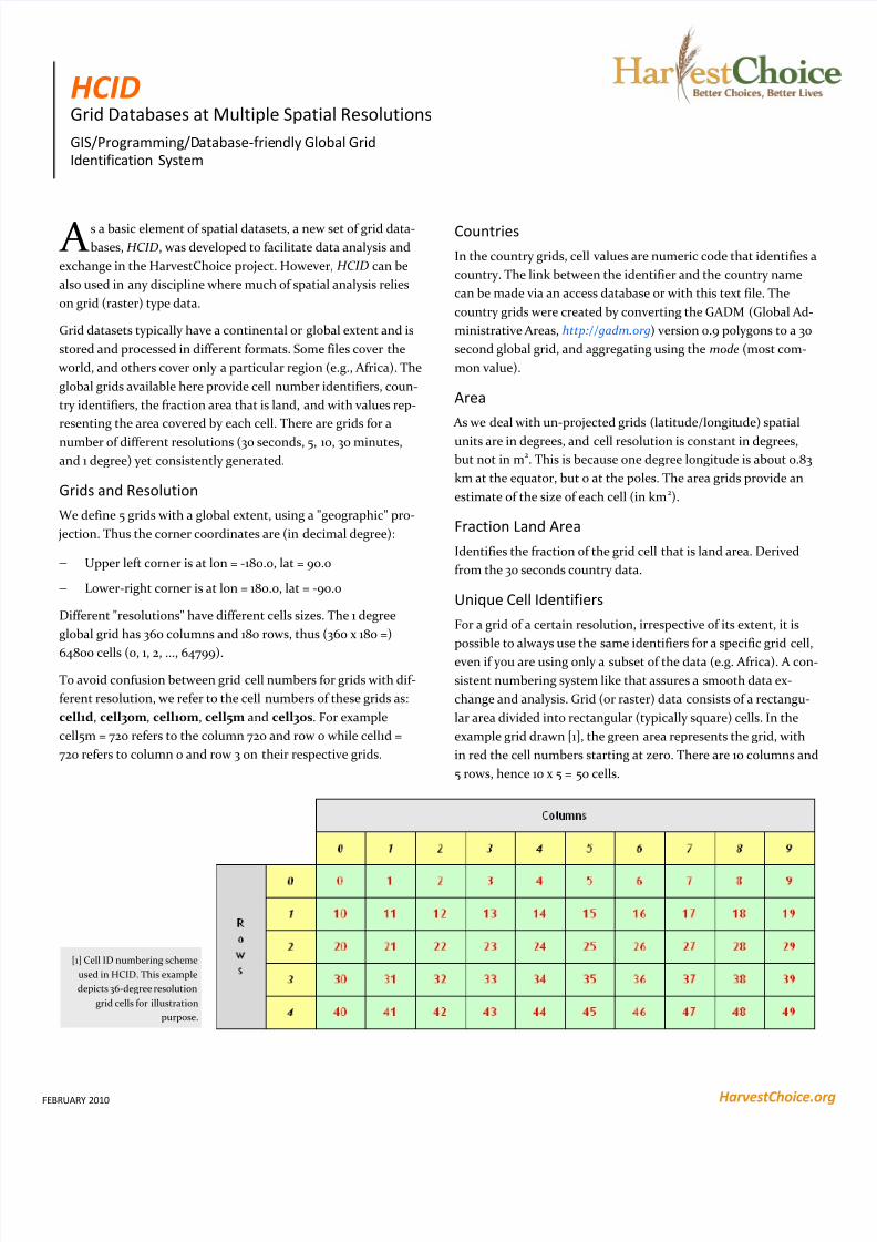
change and analysis. Grid (or raster) data consists of a rectangu-
lar area divided into rectangular (typically square) cells. In the
example grid drawn [1], the green area represents the grid, with
in red the cell numbers starting at zero. There are 10 columns and
5 rows, hence 10 x 5 = 50 cells.
HCID Grid Databases at Multiple Spatial Resolutions
GIS/Programming/Database-friendly Global Grid
Identification System
[1] Cell ID numbering scheme
used in HCID. This example
depicts 36-degree resolution
grid cells for illustration
purpose.

HarvestChoice.orgFEBRUARY 2010
The sequential numbering starts in the upper-left corner, moves
to the right, and then to the next line, to end in the lower-right
corner. For computational reasons is easier to start with 0 than
with 1 (because in most computer languages arrays are indexed
from 0...n and not from 1...n). Therefore the identifier of the last
cell will be the total number of cells minus one, which is 10 x 5 - 1
= 49 in this example. Row and column numbers also start with
zero. Cell numbers only have meaning for a specific grid
(computationally only the number of columns must be the same;
but semantically the grid also has the same spatial extent (and
resolution).
While a cell could be referred to with a row and column number,
it is in most cases much easier to have a single unique identifier
(simpler queries for example), also because for the cases where
this is necessary, computing the row or column number from a
cell number is relatively trivial. Next page shows a number of
example functions in R language that are useful in this context.
Such functions can be easily implemented in other programming
languages also.
Download
All the data files can be downloaded from the HarvestChoice Box
at: https://hc.box.net/shared/baku10bgcz
Raster
Grid cells are in the ESRI ASCII raster type format. For each reso-
lution there are three files. One file with cell numbers (filename =
"hc_seq_* "), i.e. the unique identifier for each cell. There is a also
a file indicating the country to which (the majority of) that cell
belongs (filename = "hc_cnt_* "). Countries are identified with a
numeric code that is linked to country names in the access data-
base and also here. The country grids were created by aggregat-
ing from a 30 second grid, using the mode (most common value).
Finally, there is a file in which the value represents the area of
that cell in km2 (filename = "hc_area_* ").
Vector
Same as above for the raster data, but the data are stored in a
shapefile format: hc_grid_shp.zip. That is, each raster cell is a
rectangular polygon with the cell number as an attribute for easy
(albeit perhaps inefficient) linking and displaying of data. Grid
cells that only cover oceans or seas are not included.
Cell Database
The database file (hc_grid_mdb.zip) is in the Microsoft Access
format, and it has three tables: "cells", "countries", and
" gridspecs".
Table cells links the cell numbers of the different resolutions and
also links these to the country numbers. This can be used to (dis)
aggregate data, for example to distribute data at a 1 degree resolu-
tion to different countries.
Table "countries" provides the link between the country codes
"CID" and country names. The "gridspecs" table provides some
essential parameters for each grid such as number of rows.
Country Boundaries
The country boundaries used to make the country grids is from
the GADM version 0.9.
Note
Gridded data is included for all resolutions except 30 seconds
resolution because of the large file sizes. If you require cell num-
bers of country identifiers at this resolution you can use these
grids: 30 second cell numbers (hc_seq30s_asc.zip) this one is a
very big download) and for countries (hc_cnt30s_asc.zip).
All of these files are provide for reference; in many cases using a
raster type file format and a programmatic approach to calculat-
ing cell numbers may be more efficient then linking to these files.
Screenshot of the HarvestChoice Grid Database download page

HarvestChoice.orgFEBRUARY 2010
# The below function use an grid object (list) referred to as "g". This object can be cre-
ated with this functions:
# set up a grid object (list)
setupgrid <- function(xn=-180, xx=180, yn=-90, yx=90, nr=180, nc=360) {
grid <- list(nrows=nr, ncols=nc, xmin=xn, xmax=xx, ymin=yn, ymax=yx, xres=0, yres=0)
grid$xres <- (grid$xmax - grid$xmin) / grid$ncols
grid$yres <- (grid$ymax - grid$ymin) / grid$nrows
return(grid) }
# get column number from cell number
getcolfromcell <- function(cell, g) {
if (cell >= 0 & cell < g$nrows * g$ncols) {
col <- cell - trunc(cell / g$ncols) * g$ncols }
else { col <- NA }
return(col) }
# get row number from cell number
getrowfromcell <- function(cell, g) {
if (cell >= 0 & cell < g$nrows * g$ncols) {
row <- trunc(cell / g$ncols) }
else { row <- NA }
return(row) }
# get cell number from row and column number
getcellfromrowcol <- function(row, col, g) {
if (row >= 0 & row < g$nrows & col >= 0 & col <= g$ncols) {
cell <- row * g$ncols + col}
else {cell <- NA }
return(cell) }
#To compute a cell number from a coordinate pair (x, y) you can use the functions below
# get column number from x coordinate
getcolnumber <- function(x, g) {
if ((x >= g$xmin) & (x < g$xmax)) {
return(trunc((x - g$xmin) / g$xres)) }
else { if (x == g$xmax) { return(g$ncols - 1) }
else {return(NA)} } }
# get row number from y coordinaten
getrownumber <- function(y, g) {
if ((y <= g$ymax) & (y > g$ymin)) {return(trunc((g$ymax-y) / g$yres))}
else { if (y == g$ymin) {return(g$nrows - 1)}
else {return(NA)} } }
# get cell number from x and y coordinates
getcellnumber <- function(x, y, g) {
col <- getcolnumber(x, g)
row <- getrownumber(y, g)
if ( (!is.na(col)) & (!is.na(row)) ) { return(row * g$ncols + col) }
Example R language function for grid data manipulation

HarvestChoice generates knowledge prod-
ucts to help guide strategic investments to
improve the well-being of poor people in
sub-Saharan Africa and South Asia through
more productive and profitable farming. To
do this, a novel and spatially explicit evalua-
tion framework is being developed and de-
ployed. By design, primary knowledge prod-
ucts are currently targeted to the needs of
investors, policymakers and program man-
agers, as well as the analysts and technical
specialists who support them. Most deci-
sions that HarvestChoice targets are those
having implications that cut across country
boundaries.
For further information:
Robert Hijmans
Assistant Professor | University of California Davis
Email: [email protected]
Jawoo Koo
Research fellow | International Food Policy Research Institute
Email: [email protected]