Gridded National Inventory of U.S. Methane EmissionsJoannes D. Maasakkers,*,† Daniel J. Jacob,† Melissa P. Sulprizio,† Alexander J. Turner,† Melissa Weitz,‡

Tom Wirth,‡ Cate Hight,‡ Mark DeFigueiredo,‡ Mausami Desai,‡ Rachel Schmeltz,‡ Leif Hockstad,‡

Anthony A. Bloom,¶ Kevin W. Bowman,¶ Seongeun Jeong,§ and Marc L. Fischer§

†School of Engineering and Applied Sciences, Harvard University, Pierce Hall, 29 Oxford Street, Cambridge, Massachusetts 02138,United States‡Climate Change Division, Environmental Protection Agency, Washington, District of Columbia 20460, United States¶Jet Propulsion Laboratory, California Institute of Technology, Pasadena, California 91109, United States§Energy Technologies Area, Lawrence Berkeley National Laboratory, Berkeley, California 94720, United States

ABSTRACT: We present a gridded inventory of USanthropogenic methane emissions with 0.1° × 0.1° spatialresolution, monthly temporal resolution, and detailed scale-dependent error characterization. The inventory is designed tobe consistent with the 2016 US Environmental ProtectionAgency (EPA) Inventory of US Greenhouse Gas Emissionsand Sinks (GHGI) for 2012. The EPA inventory is availableonly as national totals for different source types. We use a widerange of databases at the state, county, local, and point sourcelevel to disaggregate the inventory and allocate the spatial andtemporal distribution of emissions for individual source types.Results show large differences with the EDGAR v4.2 globalgridded inventory commonly used as a priori estimate ininversions of atmospheric methane observations. We derive grid-dependent error statistics for individual source types fromcomparison with the Environmental Defense Fund (EDF) regional inventory for Northeast Texas. These error statistics areindependently verified by comparison with the California Greenhouse Gas Emissions Measurement (CALGEM) grid-resolvedemission inventory. Our gridded, time-resolved inventory provides an improved basis for inversion of atmospheric methaneobservations to estimate US methane emissions and interpret the results in terms of the underlying processes.

■ INTRODUCTION

Under the United Nations Framework Convention on ClimateChange (UNFCCC), individual countries must report theirnational anthropogenic greenhouse gas emissions calculatedusing comparable methods.1 The Intergovernmental Panel onClimate Change (IPCC)2 provides three different methods or“tiers” for calculating emissions. All are bottom-up approachesin which emissions from individual source types are generallycalculated as the product of activity data and emission factors.Increasing tiers are more detailed and require more country-specific data. In the United States, the EnvironmentalProtection Agency (EPA) produces an annual Inventory ofUS Greenhouse Gas Emissions and Sinks (GHGI)3 forreporting to the UNFCCC. The GHGI uses detailedinformation on activity data and emission factors, generallyfollowing IPCC Tier 2 and 3 methods. It provides detailedsectoral breakdown of emissions but only reports national totalsfor most source types. Here we present a spatially disaggregatedversion of the GHGI at 0.1° × 0.1° spatial resolution andmonthly temporal resolution, including detailed informationand error characterization for individual emission types. Ourgoal is to enable the use of the GHGI as an a priori estimate for

inversions of atmospheric methane that may guide improve-ments in the inventory.Table 1 gives the GHGI estimates for 2012 with method-

ology updated in 20163 and including contributions fromdifferent source types. Total US anthropogenic emission is 29.0Tg a−1, including major contributions from natural gas systems(24%), enteric fermentation (23%), landfills (20%), coal mining(9%), manure management (9%), and petroleum (orequivalently oil) systems (8%). The inventory includes forestfire emissions but no other natural sources. The main naturalsource of methane is thought to be wetlands, accounting for 8.5± 5 Tg A−1 in the contiguous US (CONUS).4 Annualanthropogenic emissions from 1990 to 2014 computed byEPA3 with a consistent method (revised each year to includeupdated information) show no significant trend and littleinterannual variability, with US totals staying in the range 28.6-31.2 Tg a−1 and contributions from individual source typesvarying by only a few percent.

Received: June 9, 2016Revised: October 1, 2016Accepted: October 13, 2016

Article

pubs.acs.org/est

© XXXX American Chemical Society A DOI: 10.1021/acs.est.6b02878Environ. Sci. Technol. XXXX, XXX, XXX−XXX

Application of atmospheric methane observations to estimateemissions usually involves inversion of an atmospherictransport model, with consideration of a priori informationfrom an emission inventory to regularize the results and achievea Bayesian optimal estimate of emissions.5,6 The inversionoptimizes emissions on a grid, and the inventory used as apriori information must be available on that grid. In the absenceof a gridded version of the GHGI, previous inverse studies forthe US have relied on the global EDGAR inventory7 whichprovides annual emissions at 0.1° × 0.1° resolution. EDGARuses IPCC Tier 1 methods with international data sets, andonly includes a limited breakdown by source type. Nationaltotals in EDGAR are generally consistent with EPA, as shownin Table 1, but we will see that there are large errors in spatialallocation that affect inverse analyses and their interpretation.Our gridded version of the GHGI not only provides a better apriori estimate but also a better basis for interpreting inversion

results and hence improving our understanding of theunderlying processes.

■ METHODSWe disaggregate the 2012 national emissions reported by the2016 version of the GHGI3 into a gridded 0.1° × 0.1° monthlyinventory. The gridded inventory is consistent with the EPAnational emission totals for each source type (each entry inTable 1) and distributes these emissions based on informationat the state, county, subcounty, and point source levels. In thismanner, our inventory is a gridded representation of thenational GHGI. Similar disaggregation has been done fornational methane inventories in Switzerland,8,9 Australia,10 andthe United Kingdom.11 We limit our domain to the CONUS,which accounts for over 98% of total US emissions on the basisof our state-level estimates. We use the 2012 emissions fromthe 2014 EPA GHGI published in 2016, which includesdetailed descriptions of the methods used to calculate thenational emissions.3 The 2014 GHGI includes updates to thepetroleum and natural gas emissions to reflect new studies.3,12

We focus on the year 2012 as the latest year for which all spatialactivity data are available. Updating our gridded inventory tonewer iterations (the GHGI is updated annually) and lateryears will be straightforward as new activity data are released.We start from the most detailed spatial information directly

available from the GHGI. This information varies by sourcetype. Livestock emissions are available for each state, whereaswaste and petroleum systems emissions are only available asnational totals. Separate from the national inventory, EPA alsocollects methane emission and supporting data from largefacilities under the Greenhouse Gas Reporting Program(GHGRP).13 Facilities with emissions greater than 25 GgCO2 equivalent a

−1 (corresponding to 0.11 tons h−1 for a puremethane source) and subject to the applicable regulatoryrequirements must report to the GHGRP. Some emissionsreported to the GHGRP are directly measured (e.g., under-ground coal mines), while others are calculated on the basis offacility-level activity data (e.g., landfills). Where possible, we usefacility-level emissions from the GHGRP but those sometimesneed to be adjusted, as discussed below, to be consistent withthe national inventory.

Agriculture. Emissions from agriculture include entericfermentation, manure management, rice cultivation, and fieldburning of agricultural residues. EPA provides annual state-levelenteric fermentation and manure management emissions fordifferent animal types, taking into account varying practicesacross the country. We estimate county-level emissions byusing livestock numbers for 14 different animal types (includingdifferent types of cattle) from the 2012 US Department ofAgriculture Census of Agriculture for each animal type.14

County-level emissions are allocated to the 0.1° × 0.1° gridusing 9 different livestock occurrence probability maps (againdistinguishing between different types of cattle) from USDAbased on landtype.15 Emissions from enteric fermentation areassumed to have no intra-annual variability. Emissions frommanure management vary with temperature as given by16

=−⎡

⎣⎢⎤⎦⎥f

A T TRT T

exp( )m o

o m (1)

where f is a monthly scaling factor, A = 64 kJ mol−1 is theactivation energy, R is the ideal gas constant, Tm is the monthlyaverage surface skin (radiant) temperature, and To = 303 K.16

Table 1. Inventories of US Anthropogenic MethaneEmissions (Gg a−1)a

source type EPA GHGI (2012)EDGAR v4.2

(2008)

agricultureenteric fermentation 6670 (5936−7871) 6720manure management 2548 (2089−3058) 2200rice cultivation 476 (395−557) 418field burning ofagricultural residues

11 (7−15) 38

natural gas systems 6906 (5594−8978) 4758production 4442processing 890transmission and storage 1116distribution 457

wastelandfills 5691 (3528−9333) 5230

municipal 5098industrial 593

wastewater treatment 601 (367−613) 887domestic 368industrial 232

composting 77 (39−116) 83coal mines

coal mining 2658 (2339−3057) 4140underground 2159surface 499

abandoned coal mines 249 (204−309)petroleum systems 2335 (1775−5814) 1032other

forest fires 443 (62−1214) 17stationary combustion 265 (156−676) 424mobile combustion 86 (76−101) 104petrochemicalproduction

3 (1−4) 24

ferroalloy production 1 (1−1) 1total 29020 (26698−36565) 26075aColumn two shows the EPA inventory of US Greenhouse GasEmissions and Sinks (GHGI) for 2012 as updated in 2016.3 95%confidence intervals are in parentheses as provided by EPA, sometimesonly for broad source categories. Column three shows the UScomponent of the global EDGAR v4.2 inventory for 2008.7 Thegridded version of the EPA GHGI developed in this work includesseparate files for all entries in this table.

Environmental Science & Technology Article

DOI: 10.1021/acs.est.6b02878Environ. Sci. Technol. XXXX, XXX, XXX−XXX

B

Monthly emissions are calculated by scaling annual emissionswith normalized monthly f-fields using 0.625° × 0.5° monthlyaverage surface skin temperature fields from the NASAMERRA-2 meteorological data.17 Livestock emissions alsovary subanually as a function of varying herd size, andmanagement practices but those effects are not included inour inventory.Annual state-level emissions from rice cultivation are

obtained from EPA and allocated to counties using acreageharvested from the USDA Census.14 Emissions for each countyare allocated to the 0.1° × 0.1° grid based on crop maps with30 m resolution from the USDA Cropland Data Layerproduct.18 Annual emissions are then distributed overindividual months using normalized mean 2001−2010heterotrophic respiration rates from the 1° × 1° monthlyCarbon Data-Model Framework (CARDAMOM) terrestrial Ccycle analysis.19

Emissions from field burning of agricultural residues of fiveindividual crops (corn, rice, soybeans, sugar cane, and wheat)are allocated to a 2003−2007 monthly climatology ofagricultural fires.20

Natural Gas Systems. This source type includes emissionsfrom natural gas production, processing, transmission, anddistribution. It does not include emissions from abandonedwells.21 Emissions from natural gas production are availablefrom EPA for each of the six National Energy Modeling System(NEMS) regions defined by the US Energy InformationAdministration (EIA).22 The GHGI attributes emissions todifferent activities (e.g., vessel blowdowns, well workovers,liquid unloading) and equipment (e.g., pneumatic devices).Detailed maps of these activities and equipment are notavailable. Therefore, we rely on monthly well data obtainedfrom DrillingInfo.23 Separate DrillingInfo data are available forthe number of gas producing wells, nonassociated gas wells(gas-to-oil ratio over 100 mcf gas per barrel), coalbed methanewells, and coalbed methane well water production. We alsodistinguish conventional and unconventional wells as someemissions are specific to hydraulic fracturing. A well is flaggedas unconventional if the drilling direction is horizontal as givenby DrillingInfo or if the reservoir type is coalbed, lowpermeability, or shale.3 For each NEMS region, we allocateemissions using the DrillingInfo-based maps best representativeof the spatial distribution of the considered activity orequipment. State-level condensate production from EIA24 iscombined with nonassociated gas well maps to allocateemissions from condensate tank vents. Three gas-producingstates (Illinois, Indiana, and Tennessee) do not have activewells in the DrillingInfo database and amount to less than 1%of national active gas wells.25 For these states we use state-leveldata on the number of natural gas wells25 to calculate stateemissions and then use county-level gas production26 andfinally three different well databases to grid emissions.27−29 Foroffshore emissions, the 2011 Gulfwide Offshore Activity DataSystem (GOADS) platform-level emission database is used forthe Gulf of Mexico3,30 and DrillingInfo is used outside of theGulf of Mexico, scaling total emissions to the national emissionfrom the GHGI. As no national spatial data are available forgathering processes (only a subset report to the GHGRP31),emissions from these processes are included in the productionsector and gridded in the same way.Emissions from gas processing are only available as national

totals in the GHGI. We allocate emissions to processing plantsby combining the GHGRP data13 with the EIA database for

these plants.32 The GHGRP covers 85% of the processed gasflow from the EIA database. For the remaining plants in theEIA database, emissions are estimated by multiplying their gasflow with the average ratio of methane emissions to gas flow ofthe GHGRP plants. Subsequently, emissions from all plants arescaled to match the national GHGI number; the scaling isrequired because the GHGRP does not include all emittingprocesses occurring at the plants and has different emissionestimates per process.31 Thus, we only use the GHGRP toallocate emissions in a relative sense with emission magnitudesconstrained by the GHGI. The EIA database only providespostal codes for the processing plants and not coordinates; wedetermine non-GHGRP plant coordinates from the RextagStrategies US Natural Gas Pipeline and Infrastructure WallMap.33 If there is no match with the GHGRP or Rextag data,emissions from the plant in the EIA database are spread outover the associated postal code area.34

EPA provides national emissions for different parts of thetransmission sector. Most important are transmission com-pressor stations, for which we use a similar mapping as forprocessing plants. The GHGRP data for individual compressorstations are complemented with the EIA database fornonreporting compressor stations.35 Emissions for nonreport-ing compressor stations are estimated based on theirthroughput,35 using the average ratio of throughput to methaneemission from the GHGRP data. Emissions are then scaled tothe national total so our results are not affected by potentialunderestimates in the GHGRP emissions.36 Similarly, adatabase of storage stations37 is combined with the GHGRPusing total field capacity to predict emissions. Locations arebased on the GHGRP, supplemented by gas storage fieldlocations georeferenced from the Rextag Strategies US NaturalGas Pipeline and Infrastructure Wall Map,33 and DrillingInfo.23

Similar approaches are also used for liquid natural gas (LNG)storage38 and LNG import terminals.39 Emissions from pipelineleaks and transmission meter and regulator stations areallocated to the network of interstate and intrastate pipelines.40

Emissions from farm taps are allocated to pipelines intersectingwith agricultural land.18 Emissions related to storage at wells aremapped to all nonassociated gas wells.23

Emissions from different parts of the distribution network areavailable from EPA as national estimates. State-level emissionsfrom distribution pipeline leaks are calculated using state dataon pipeline miles and services from the Pipeline and HazardousMaterials Safety Administration (PHMSA) of which the sum isused for the national GHGI.41 This takes into account differentmaterials (e.g., cast iron, plastic) with different emission factors.Emissions from distribution meter and regulator stations aredivided among states using state-level aggregated GHGRPinformation (no finer spatial information is available). Otherdistribution emissions are partitioned between the states basedon leaked gas volume data from EIA.42 Within states, emissionsare mapped to 0.1° × 0.1° population data from the 2010 USCensus.43

Waste. Waste emissions include landfills, wastewatertreatment, and composting, for which EPA provides nationaltotals following the categories in Table 1. We allocate emissionsfrom landfills based on a combination of data from the GHGRP(1231 municipal landfills, 175 industrial landfills), the LandfillMethane Outreach Program (LMOP, municipal landfillsonly),44 and the Facility Registration Service (FRS).45

GHGRP landfills are assigned their reported emissions. 900of 2049 LMOP landfills do not report emissions to the

Environmental Science & Technology Article

DOI: 10.1021/acs.est.6b02878Environ. Sci. Technol. XXXX, XXX, XXX−XXX

C

GHGRP. For those we estimate emissions from GHGRP-reporting landfills with similar attributes (presence of acollection system, flares). Some landfills report landfill gasproduction through the LMOP. For the other landfills, waste inplace is used as estimation metric combined with a decay factorfor landfills that closed before 2012.46 For landfills without anydata (108), we assign the median emissions from the landfillsfor which information was available. Finally, we use landfillswith known coordinates from the FRS that are not present inthe GHGRP or LMOP data sets. We decide whether a landfillis municipal or industrial based on keyword descriptors in thedatabases. The 722 municipal FRS landfills are assigned themedian emission derived from above, after which all non-GHGRP emissions are scaled to match the national emissionestimate. For industrial landfills, the national estimate minusthe GHGRP emissions is uniformly allocated across the 2309industrial landfills from the FRS.Emissions from wastewater treatment are reported as

municipal or industrial in the GHGI. Facilities that report tothe GHGRP account for 84% of the national industrialwastewater treatment emissions. To allocate the remainingindustrial emissions as well as the municipal emissions, we usefacility-level wastewater flow data from the Clean WatershedsNeeds Survey.47 Industrial wastewater treatment emissions aremapped to treated industrial flow, emissions from municipalseptic systems to decentralized municipal flow, and centralizedmunicipal systems emissions to centralized municipal flow.State-level emissions from composting are calculated using

the tonnage of municipal solid waste composted or, ifcomposting data are not available, from the correlated tonnagerecycled.48 Within states, emissions are allocated to locationsfrom the US Composting Council,49 BioCycle composterdatabase,50 and composting entries in the FRS.45 If there arefewer than three facilities found in a state, we allocate based ongridded population instead.43

Coal Mines. We allocate coal mining emissions using state-level emission estimates produced for the GHGI (M. Cote,́Ruby Canyon Engineering, unpublished data) for undergroundmines and surface mines. These estimates account for methanerecovered or destroyed, as well as postmining emissions(methane released during coal handling and processing). Weuse the locations and production of all active surface andunderground coal mines from EIA.51 A large number ofunderground mines report their annual methane emissions toGHGRP. We estimate emissions from nonreporting under-ground mines based on their share of the state total coalproduction combined with the state-level emissions, weightedby the basin-level in situ methane content of the coal for statesthat have mines in multiple basins.3 Subsequently, we scale theemissions from nonreporting mines so that the total nationalemissions (including the GHGRP mines) match the GHGI.For surface mines, no GHGRP data are available. Emissions areallocated using the EPA state-level data as given above,combined with EPA basin-level emission factors and EIAmine-level production data. Similarly, postmining emissions areallocated to all mines based on their production and basin-specific emission factors.The GHGI also includes emissions from abandoned coal

mines. We start from the Abandoned Coal Mine MethaneOpportunities Database (ACMMOD)52 and add recentlyclosed coal mines plus county-level estimates of mine closuresbefore 1972 not included in ACMMOD (unpublished dataproduced for EPA by Ruby Canyon Engineering). For all

closed mines, estimates of closure dates, status (venting, sealed,flooded), and estimates of emissions when the mine was activeare available or estimated from county-level averages, allowingthe estimation of present-day emissions based on declineequations used in the GHGI.53 ACMMOD only includes minelocations on the county level. Precise locations of approx-imately one-third of the abandoned mines are found in the FullMine Info data set.54 The remaining emissions are allocated onthe county level.

Petroleum Systems. The GHGI includes nationalemissions from different activities and equipment related topetroleum production, refining, and transport. We use monthlywell data for several production quantities from DrillingInfo23

to spatially allocate these emissions. These include total, heavy,and light oil production, with the cutoff between the last two atan American Petroleum Institute (API) gravity of 20. EPAestimates some emissions separately for heavy and light oilproduction. Furthermore, we created maps of oil wells (definedas wells with a produced gas-to-oil ratio under 100 mcf perbarrel, wells with a higher ratio are classified as nonassociatedgas wells), stripper wells (producing fewer than 10 barrels perday), and total and unconventional oil well completions. Similarto the allocation of natural gas production emissions, stateswithout active wells in DrillingInfo are represented using state-specific data sets and amount to less than 1% of nationalproduction.55 For the other states, the national-level emissionsfrom each activity and device are allocated using theDrillingInfo maps. For example, emissions from well drillingare mapped to well completions, while emissions from heavycrude oil wellheads are mapped to heavy oil wells. As for naturalgas systems, offshore emissions are based on the GOADSdatabase for the Gulf of Mexico and DrillingInfo elsewhere.Emissions from petroleum refining are allocated to GHGRPfacilities based on their reported emissions. National emissionsfrom petroleum transportation are divided between the wells,offshore platforms, and refineries.

Other. Other refers to a number of smaller sources listed inTable 1. National forest fire emissions from the GHGI aredistributed on a daily basis at 0.1° × 0.1° resolution using theQuick Fire Emissions Data set (QFED v2.4) for 2012.56

Stationary combustion emissions from electricity generation arecalculated by multiplying plant-level heat inputs from the AcidRain Program with fuel type specific emission factors.57

Additional stationary combustion emissions from the industrial,commercial, and residential sectors are based on state-levelconsumption of different types of fuel (coal, fuel oil, natural gas,and wood) as reported by EIA.58 Within states, residential andcommercial emissions are allocated based on population whileindustrial emissions are allocated based on combustionemissions reported to the GHGRP. National on-road mobilecombustion emissions for individual vehicle types in the GHGIare allocated spatially by first calculating state-level vehicle milestraveled (VMT) for six types of roads: urban and rural for eachof primary, secondary, and other (minor) roads59 andattributing those to individual vehicle types.59 These statetotals are then mapped to the different road networks takenfrom the National Transportation Atlas60 and US Censusproducts.61 Combustion emissions from rail transport areallocated over the US railroad network.61 Emissions fromagricultural equipment are uniformly spread out across allagricultural land.18 Emissions from mining-related vehicles areallocated to active mines.54 Construction and “other” mobilecombustion emissions are mapped based on population.

Environmental Science & Technology Article

DOI: 10.1021/acs.est.6b02878Environ. Sci. Technol. XXXX, XXX, XXX−XXX

D

National emissions from ferroalloy production and from thepetrochemical industry are divided over the facilities reportingto the GHGRP based on their total reported emissions.

■ RESULTS AND DISCUSSIONFigure 1 shows the distribution of annual emissions on the 0.1°× 0.1° grid for the six general emission categories of the

Methods section. Emissions from agriculture are broadlydistributed across livestock farming areas. Hotspots are mostlyfrom concentrated dairy cattle or hog populations such as inIowa, North Carolina, and California. Rice cultivationcontributes hotspots in northern California and along thelower Mississippi River. Emissions from natural gas systems arehigh in production fields, for example in Pennsylvania(Marcellus shale) and in Texas, with a maximum at FourCorners as found in top-down studies.62 Waste emissions(dominated by landfills; Table 1) roughly map to population,with hotspots from large landfills and wastewater facilities. Coalmining emissions are concentrated in Appalachia. Petroleumsystems emissions peak over the Bakken region in NorthDakota and western Texas where natural gas emissions are low.Other emissions mostly feature forest fire hotspots in the Westand stationary combustion emissions in populated areas.Total CONUS emissions for 2012 are 28.7 Tg a−1, slightly

lower than the 29.0 Tg a−1 national total reported in Table 1because of contributions from Alaska, Hawaii, and outsideterritories. Several sources vary monthly in our inventoryincluding manure management, natural gas and petroleumproduction, stationary combustion, and forest fires (daily).Monthly emissions vary from 73 Gg per day in December to 89Gg per day in July. Most of this monthly variation arises frommanure management, which varies nationally from 2.4 Gg perday in January to 16.8 Gg per day in July. Eq 1 is for liquid

storage systems but is applied here to all manure managementsystems, which may overestimate the seasonal variation.63,64

For rice emissions, we assume a constant methane to CO2emission ratio from heterotrophic respiration, which mayunderestimate the seasonal variation as the ratio has been foundto increase with temperature in wetlands and aquaticecosystems.65 On the other hand, some seasonal factors arenot considered in our inventory due to lack of data such aslivestock numbers, feed, and gas/petroleum distribution.Transient elevated emissions from oil/gas systems (the so-called “super-emitters”66) are also not resolved.Figure 2 compares the distribution of total methane

emissions in our gridded EPA inventory for 2012 to theEDGAR v4.2 inventory for 2008, the latest year of full release.7

A fast track version of EDGAR (v4.2 FT20107) has come outsince but, based on visual inspection, the spatial emissionspatterns in EDGAR v4.2 are of higher quality and most inversestudies have used EDGAR v4.2. There are large differences inspatial patterns between the Gridded EPA inventory andEDGAR v4.2, particularly for oil/gas systems and manuremanagement. Emissions in the gridded EPA inventory aremuch higher over oil/gas production areas and lower overdistribution (populated) areas. The two inventories show nosignificant correlation at their native 0.1° × 0.1° resolution (r =0.06). The correlation increases to r = 0.42 at 0.5° × 0.5°resolution and r = 0.63 at 1.0° × 1.0° resolution.Previous inverse studies for US methane emissions using

EDGAR as a priori estimate have all found the need for a largeupward correction of emissions in the South-Central US.67−70

Figure 3 shows the distributions of livestock, oil/gas systems,and waste emissions for that region in the gridded EPA andEDGAR v4.2 inventories. The EDGAR v4.2 inventory placesthe oil/gas emissions in urban areas and completely missesareas of production. The oil/gas emissions in EDGAR v4.2 arestrongly correlated with waste emissions because both arelargely distributed following population. An inversion usingEDGAR v4.2 as a priori estimate would not be able to separatethe two and might wrongly attribute a source in oil/gasproduction regions to livestock. This stresses the importance ofusing a high-quality a priori inventory in inverse analyses, bothto regularize the solution and to enable interpretation of results.Whereas different source types show spatial correlation in theEDGAR v4.2 inventory because of mapping to commondatabases, there is no such correlation between source types inour gridded EPA inventory even at 1° × 1° resolution. Thisseparation between individual source types holds promise forinterpreting results from inverse analyses.Error characterization is necessary for a gridded emission

inventory to serve as a priori estimate in Bayesian inversionsand to interpret results from the inversions. Error character-ization is not available for the EDGAR v4.2 inventory andinversions have typically assumed 30−100% uniform errorbased on expert judgment, or used the inversion to estimate theerror in the a priori.71 The GHGI includes detailed errorcharacterization on its national totals for individual sourcetypes, based on propagation of uncertainties in the constructionof the bottom-up estimates (Table 1). Errors in our 0.1° × 0.1°gridded inventory may be larger because of local uncertaintiesin activity data and emission factors, including the preciselocalization of emissions. For the same reason, averaging ourinventory over coarser grids (by adding contributions from 0.1°× 0.1° grid cells) could reduce the error. This scale dependenceis important to describe because inversions may seek to

Figure 1. Contiguous US (CONUS) methane emissions fromdifferent source categories. Total annual US emissions from the2016 EPA GHGI for 2012 are disaggregated here on a 0.1° × 0.1° grid.“Other” refers to the ensemble of minor sources in Table 1. (Anequivalent figure for EDGAR v4.2 is shown by in Turner et al.70).

Environmental Science & Technology Article

DOI: 10.1021/acs.est.6b02878Environ. Sci. Technol. XXXX, XXX, XXX−XXX

E

optimize emissions at different spatial resolutions depending onthe information content of the atmospheric observations.Here we derive scale-dependent error statistics for our

gridded EPA inventory by comparison to a detailed bottom-upemission inventory compiled by Environmental Defense Fund(EDF) for the ∼300 × 300 km2 Barnett Shale region inNortheast Texas by Lyon et al.72 and subsequently updatedwith top-down constraints by Zavala-Araiza et al.73 The EDFinventory was constructed largely independently from theGHGI. It is based on an extensive field campaign in the region

in September−October 2013 including measurements ofindividual facilities as well as regional surveys.12 The BarnettShale region is of particular interest as a comparison standardbecause it includes diverse sources: the largest oil/gas field inthe CONUS (30 000 active wells), major livestock operations,and the metropolitan area of Dallas/Fort Worth. The EDFinventory incorporates considerable local information that goesbeyond the databases used in constructing our inventory, andincluding for example precise locations of dairy farms, gasgathering stations, and landfills.72 Emissions are reported on a 4× 4 km2 grid (approximately 0.04° × 0.04°) with detailedbreakdown by source types and statistical sampling of “super-emitter” facilities with anomalously large emissions.Figure 4 shows emissions from livestock, natural gas, waste,

and petroleum in the Zavala-Araiza EDF Barnett Shaleinventory and compares to our gridded EPA inventory.Emission totals for the domain are shown in Table 2. Thereis a large difference in the magnitude of the source from oil/gasproduction, at least in part because Zavala-Araiza et al. find alarger frequency of superemitters than assumed in the GHGIemission factors. Despite this difference in magnitude there is astrong spatial correlation on the 0.1° × 0.1° grid (r = 0.78),implying that correction to the gridded EPA distribution in aninversion of atmospheric data could be reliably attributed to theoil/gas production source type, smoothing temporally oversuperemitters. The spatial correlation coefficient of thelivestock source between the gridded EPA and EDF inventoriesis only 0.37 at 0.1° × 0.1° resolution but increases to 0.88 at0.5° × 0.5° resolution. The gridded EPA inventory misses theexact locations of farms but this error is smoothed out on thecounty scale.We take the Zavala-Araiza EDF Barnett Shale inventory as

our best approximation of emissions in the region in order toderive scale-dependent error statistics for different source typesthat can be used in an inversion of atmospheric concentrationdata. We assume for this purpose that the total error probabilitydensity function (pdf) for each source type in a given grid cell isGaussian and includes a displacement error due to impreciselocalization. Our error model is given by

∑σ αβ

= ′ −∥ − ′∥

′

⎛⎝⎜

⎞⎠⎟Ex x

x x( ) ( ) exp

x

22

2

2

(2)

Here, σ(x) is the Gaussian error standard deviation for the gridcell centered at location x and for a given source type, α is abase relative error standard deviation assuming no displacementerror, E(x′) is the 2-D field of emissions for that source typeover all grid cells, and β is a length scale for the displacementerror. α and β are assumed to be uniform for a given sourcetype. We find optimal values for α and β by minimizing a least-squares cost function J(α, β) for the difference between ourestimated error standard deviation and the absolute differencebetween the gridded EPA and EDF emissions:

∑α β σ α β= − | − |J E Ex x x( , ) ( ( , , ) ( ) ( ) )x

EDF2

(3)

where the summation is over all grid cells of the Barnett Shaledomain in Figure 4. Optimization of α and β is done for thedifferent source types of Figure 4 (also separating waste aslandfills and wastewater) and for grid resolutions L from 0.1° to0.5° to determine the scale dependence of the error. 0.5° is thecoarsest scale that can be usefully constrained from the BarnettShale inventory, but from there we can extrapolate to the

Figure 2. Total methane emissions in the gridded EPA inventory for2012 (top), EDGAR v4.2 for 2008 (middle), and difference betweenthe two (bottom).

Environmental Science & Technology Article

DOI: 10.1021/acs.est.6b02878Environ. Sci. Technol. XXXX, XXX, XXX−XXX

F

national scale using the GHGI error estimates. For this purposewe take the average of the upper and lower confidence intervalsfor the given source type in Table 1 as representing the relativeerror standard deviation αN on the national scale. We then fitour results for α(L) and β(L) to exponential forms of L, withasymptote αN for α. This yields

α α α= − − +αk L Lexp( ( )) N0 0 (4)

β β= − −βk L Lexp( ( ))0 0 (5)

Here L0 = 0.1° is the native resolution of our inventory, and kαand kβ (in units of inverse degrees) are smoothing coefficientsthat express the scale dependence of the error. The fit is subjectto the condition α0 ≥ 0; if the base error standard deviationderived from the Barnett Shale inventory is smaller than αNthen we assume that α is scale-independent and equal to αN.Figure 5 shows the base relative error standard deviation α

and displacement length scale β as a function of grid resolutionL for the different source types active in the Barnett Shale.Values for all coefficients in eqs 4 and 5 are given in Table 3.Base error standard deviations (α) for different source types at

Figure 3. Emissions from livestock, oil/gas systems, and waste over the South-Central US in the gridded EPA inventory for 2012 and the EDGARv4.2 inventory for 2008.

Figure 4. Methane emissions in the Barnett Shale region of Northeast Texas. Values for the four main categories are shown for our gridded EPAinventory and for the EDF inventory73 at 0.1° × 0.1° resolution. The original EDF inventory is at 4 × 4 km2 and is regridded here to 0.1° × 0.1° forcomparison with our inventory. The location of the Barnett Shale region is shown inset. Emission totals for the region are given in Table 2.

Environmental Science & Technology Article

DOI: 10.1021/acs.est.6b02878Environ. Sci. Technol. XXXX, XXX, XXX−XXX

G

0.1° × 0.1° grid resolution are all above 50%. Errors forlivestock, natural gas systems, and wastewater are scale-dependent and decrease when coarser grid resolutions areused. Errors for petroleum systems and landfills are defined bythe national estimates, which are relatively large, and are thusscale-independent. The displacement error measured by β isusually very small, less than 0.1°, in part because it is isotropic(there is no a priori information on the direction of

displacement error). Because of its Gaussian form, itemphasizes the effect of neighboring misplacements; it wouldnot capture the error from a distant misplacement or from acompletely missing source.We recommend that users of our emission inventory at a

given grid resolution L apply the error parameters in Table 3nationally to derive α(L) and β(L) from eqs 4 and 5, and fromthere use eq 2 to derive the absolute error standard deviation σfor individual source types and grid cells. For source types notconstrained by the Barnett Shale inventory, we assume herethat the base error standard deviation at 0.1° × 0.1° resolutionis 2.5 times the national value from Table 1, based on themedian scale dependence for the sources in the Barnett Shale.We use median values of the other error parameters in Table 3and cap α at 1.0. Error variances for the different source typespresent in a grid cell can be added in quadrature to derive theerror variance for the total emission in that grid cell. A simplevariogram analysis76 of the difference between the EDF andEPA inventories shows no spatial error correlation, either fortotal emissions or for individual source types, suggesting thatthe a priori error covariance matrix needed for a Bayesianinversion can be assumed diagonal. A previous study comparinga disaggregated national inventory for Switzerland to EDGARv4.2 did find significant spatial error correlations.8

Table 2. Regional Methane Emissions (Gg a−1)a

Barnett Shale region California

source EDF (Lyon) EDF (Zavala-Araiza) this work r CALGEM this work r

oil/gas production 330 436 327 0.78 171 264 0.90gas processing 49 65 62 0.24 12 7 0.25gas transmission 16 2 8 0.20 22 24 0.69gas distribution 10 9 16 0.87 131 39 0.98livestock 104 102 122 0.37 721 885 0.46landfills 105 99 92 0.76 316 507 0.86wastewater 7 7 12 0.21 91 45 0.53sum 621 720 640 0.68 1463 1772 0.66

aAnthropogenic emissions from the Barnett Shale region in Northeast Texas (Figure 4) and from the state of California (Figure 6). Regional totalsby source type from our gridded version of the gridded EPA inventory for 2012 (this work) are compared to the original bottom-up (Lyon) EDFinventory for the Barnett Shale in October 2013,72 the updated (Zavala-Araiza) EDF inventory including top-down information,73 and the CALGEMinventory for California in 2008 (livestock/waste)63,74 and 2010 (oil/gas).75 Also shown are spatial correlation coefficients r on the 0.1° × 0.1° gridfor the Barnett Shale73 and 0.2° × 0.2° for California.

Figure 5. Relative error standard deviations for methane emissions from individual source types and their scale dependences. The figure shows theerror parameters α and β used in eq 2 to calculate the absolute error standard deviations for a given L × L grid cell and source type as a function ofthe grid resolution L. The native grid resolution of the inventory is 0.1° × 0.1°, and averaging over coarser scales decreases errors for individualsource types as described by exponential decay functions (eqs 4 and 5). The asymptotes for the base error standard deviations are the national valuesαN shown as tick marks on the right side of the left panel. Values for all error parameters are given in Table 3.

Table 3. Error Parameters for the Gridded EPA EmissionInventory

source α0 kα αN β0 kβ

livestock 0.89 3.1 0.12 0natural gas systems 0.28 4.2 0.25 0.09 3.9landfills 0 0.51 0.08 2.0wastewater treatment 0.78 1.4 0.21 0.06 6.9petroleum systems 0 0.87 0.04 197

aError parameters for use in eqs 4 and 5 to compute the base relativeerror standard deviation α(L) and displacement error length scaleβ(L) for different source types at different grid resolutions L × L. Theresulting values of α(L) and β(L) should be used in eq 2 to estimatethe error standard deviation for a given source type and grid cell. Unitsare degrees for L and β0, and inverse degrees for kα and kβ. α0 and αNare dimensionless. The livestock error estimate is to be applied to thesum of enteric fermentation and manure management emissions.

Environmental Science & Technology Article

DOI: 10.1021/acs.est.6b02878Environ. Sci. Technol. XXXX, XXX, XXX−XXX

H

Our error model is a first attempt to quantify grid-dependenterrors for use in inversions of atmospheric concentration data,and in that it significantly improves on previous bottom-upinventories. It has however a number of weaknesses. First, theBarnett Shale region may not be representative nationally andoffers no error characterization for some sources (in particularcoal mining). Second, inverse analyses of atmosphericobservations67,70,77 suggest that EPA underestimates on thenational scale maybe be larger than estimated from αN,although these inverse analyses have their own errors. Third,the assumed Gaussian form for the error pdf is convenient foranalytical inversions6 but is not optimal. It does not excludeunphysical negative solutions and it does not capture the “fattail” of the pdf contributed by superemitters.66,72 A log-normalerror pdf would solve the positivity problem and allow a betterdescription of the fat tail. Fourth, some spatial error correlationwould be expected even though it cannot be detected in oursimple variogram analysis for the Barnett Shale; more advancedvariogram analyses and better data sets might enabledetection.8,76 Fifth, we do not consider temporal errorcorrelations because inversions typically focus on optimizingthe spatial distribution while assuming the temporal variation tobe known (and relatively weak in our case). This may not beappropriate for some applications, in particular whenoptimizing emissions from seasonally varying sources.19

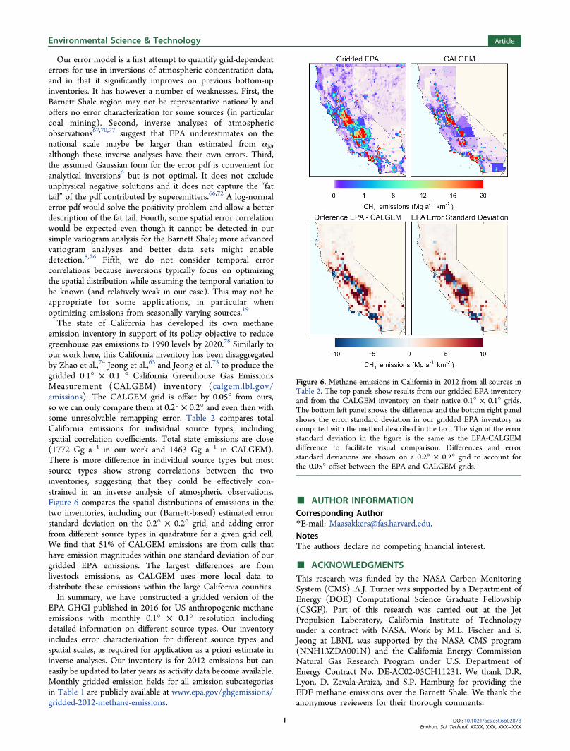
The state of California has developed its own methaneemission inventory in support of its policy objective to reducegreenhouse gas emissions to 1990 levels by 2020.78 Similarly toour work here, this California inventory has been disaggregatedby Zhao et al.,74 Jeong et al.,63 and Jeong et al.75 to produce thegridded 0.1° × 0.1 ° California Greenhouse Gas EmissionsMeasurement (CALGEM) inventory (calgem.lbl.gov/emissions). The CALGEM grid is offset by 0.05° from ours,so we can only compare them at 0.2° × 0.2° and even then withsome unresolvable remapping error. Table 2 compares totalCalifornia emissions for individual source types, includingspatial correlation coefficients. Total state emissions are close(1772 Gg a−1 in our work and 1463 Gg a−1 in CALGEM).There is more difference in individual source types but mostsource types show strong correlations between the twoinventories, suggesting that they could be effectively con-strained in an inverse analysis of atmospheric observations.Figure 6 compares the spatial distributions of emissions in thetwo inventories, including our (Barnett-based) estimated errorstandard deviation on the 0.2° × 0.2° grid, and adding errorfrom different source types in quadrature for a given grid cell.We find that 51% of CALGEM emissions are from cells thathave emission magnitudes within one standard deviation of ourgridded EPA emissions. The largest differences are fromlivestock emissions, as CALGEM uses more local data todistribute these emissions within the large California counties.In summary, we have constructed a gridded version of the

EPA GHGI published in 2016 for US anthropogenic methaneemissions with monthly 0.1° × 0.1° resolution includingdetailed information on different source types. Our inventoryincludes error characterization for different source types andspatial scales, as required for application as a priori estimate ininverse analyses. Our inventory is for 2012 emissions but caneasily be updated to later years as activity data become available.Monthly gridded emission fields for all emission subcategoriesin Table 1 are publicly available at www.epa.gov/ghgemissions/gridded-2012-methane-emissions.

■ AUTHOR INFORMATIONCorresponding Author*E-mail: Maasakkers@fas.harvard.edu.NotesThe authors declare no competing financial interest.

■ ACKNOWLEDGMENTSThis research was funded by the NASA Carbon MonitoringSystem (CMS). A.J. Turner was supported by a Department ofEnergy (DOE) Computational Science Graduate Fellowship(CSGF). Part of this research was carried out at the JetPropulsion Laboratory, California Institute of Technologyunder a contract with NASA. Work by M.L. Fischer and S.Jeong at LBNL was supported by the NASA CMS program(NNH13ZDA001N) and the California Energy CommissionNatural Gas Research Program under U.S. Department ofEnergy Contract No. DE-AC02-05CH11231. We thank D.R.Lyon, D. Zavala-Araiza, and S.P. Hamburg for providing theEDF methane emissions over the Barnett Shale. We thank theanonymous reviewers for their thorough comments.

Figure 6. Methane emissions in California in 2012 from all sources inTable 2. The top panels show results from our gridded EPA inventoryand from the CALGEM inventory on their native 0.1° × 0.1° grids.The bottom left panel shows the difference and the bottom right panelshows the error standard deviation in our gridded EPA inventory ascomputed with the method described in the text. The sign of the errorstandard deviation in the figure is the same as the EPA-CALGEMdifference to facilitate visual comparison. Differences and errorstandard deviations are shown on a 0.2° × 0.2° grid to account forthe 0.05° offset between the EPA and CALGEM grids.

Environmental Science & Technology Article

DOI: 10.1021/acs.est.6b02878Environ. Sci. Technol. XXXX, XXX, XXX−XXX

I

■ REFERENCES(1) United Nations. United Nations Framework Convention onClimate Change, Article 4(1)(a), , 1992. unfccc.int.(2) IPCC. Guidelines for National Greenhouse Gas Inventories;Eggleston, H. S., Buendia, L., Miwa, K., Ngara, T., Tanabe, K., Eds.;The National Greenhouse Gas Inventories Programme: Hayama,Kanagawa, Japan, 2006.(3) EPA. Inventory of US Greenhouse Gas Emissions and Sinks:1990−2014, 2016. https://www.epa.gov/ghgemissions/us-greenhouse-gas-inventory-report-1990-2014.(4) Melton, J.; Wania, R.; Hodson, E.; Poulter, B.; Ringeval, B.;Spahni, R.; Bohn, T.; Avis, C.; Beerling, D.; Chen, G.; et al. Presentstate of global wetland extent and wetland methane modelling:conclusions from a model intercomparison project (WETCHIMP).Biogeosciences 2013, 10, 753−788.(5) Streets, D. G.; Canty, T.; Carmichael, G. R.; de Foy, B.;Dickerson, R. R.; Duncan, B. N.; Edwards, D. P.; Haynes, J. A.; Henze,D. K.; Houyoux, M. R.; et al. Emissions estimation from satelliteretrievals: A review of current capability. Atmos. Environ. 2013, 77,1011−1042.(6) Jacob, D. J.; Turner, A. J.; Maasakkers, J. D.; Sheng, J.; Sun, K.;Liu, X.; Chance, K.; Aben, I.; McKeever, J.; Frankenberg, C. Satelliteobservations of atmospheric methane and their value for quantifyingmethane emissions. Atmos. Chem. Phys. Discuss. 2016, 2016, 1−41.(7) European Commission. Emission Database for Global Atmospher-icResearch (EDGAR), 527 release version 4.2.; European Commission,2011.(8) Hiller, R.; Bretscher, D.; DelSontro, T.; Diem, T.; Eugster, W.;Henneberger, R.; Hobi, S.; Hodson, E.; Imer, D.; Kreuzer, M.; et al.Anthropogenic and natural methane fluxes in Switzerland synthesizedwithin a spatially explicit inventory. Biogeosciences 2014, 11, 1941−1959.(9) Henne, S.; Brunner, D.; Oney, B.; Leuenberger, M.; Eugster, W.;Bamberger, I.; Meinhardt, F.; Steinbacher, M.; Emmenegger, L.Validation of the Swiss methane emission inventory by atmosphericobservations and inverse modelling. Atmos. Chem. Phys. 2016, 16,3683−3710.(10) Wang, Y.-P.; Bentley, S. Development of a spatially explicitinventory of methane emissions from Australia and its verificationusing atmospheric concentration data. Atmos. Environ. 2002, 36,4965−4975.(11) Defra. National Atmospheric Emissions Inventory, 2014. naei.defra.gov.uk.(12) Harriss, R.; Alvarez, R. A.; Lyon, D.; Zavala-Araiza, D.; Nelson,D.; Hamburg, S. P. Using multi-scale measurements to improvemethane emission estimates from oil and gas operations in the BarnettShale region, Texas. Environ. Sci. Technol. 2015, 49, 7524−7526.(13) EPA. Greenhouse Gas Reporting Program, 2013. epa.gov/ghgreporting/.(14) USDA. Census of Agriculture; USDA-NASS: Washington, DC,2012; quickstats.nass.usda.gov.(15) USDA. Census of Agriculture: Weighted Land Use/Cover FilterFiles; USDA-NASS: Washington, DC, 2012; agcensus.usda.gov/Publications/2012/Online_Resources/Ag_%20551%20Atlas_Maps/.(16) Mangino, J.; Bartram, D.; Brazy, A. Development of a methaneconversion factor to estimate emissions from animal waste lagoons.Presented at the US EPA 17th Emission 554 Inventory Conference,Atlanta, GA, April 2002.(17) Bosilovich, M. G.; Lucchesi, R.; Suarez, M. File Specification forMERRA-2. GMAO Office Note No. 9 (Version 1.1), 2016. gmao.gsfc.nasa.gov/pubs/docs/Bosilovich785.pdf.(18) USDA. Cropland Data Layer; USDA-NASS: Washington, DC,2014; nassgeodata.gmu.edu/CropScape/.(19) Bloom, A. A.; Exbrayat, J.-F.; van der Velde, I. R.; Feng, L.;Williams, M. The decadal state of the terrestrial carbon cycle: Globalretrievals of terrestrial carbon allocation, pools, and residence times.Proc. Natl. Acad. Sci. U. S. A. 2016, 113, 1285−1290.

(20) McCarty, J. L. Remote sensing-based estimates of annual andseasonal emissions from crop residue burning in the contiguousUnited States. J. Air Waste Manage. Assoc. 2011, 61, 22−34.(21) Kang, M.; Kanno, C. M.; Reid, M. C.; Zhang, X.; Mauzerall, D.L.; Celia, M. A.; Chen, Y.; Onstott, T. C. Direct measurements ofmethane emissions from abandoned oil and gas wells in Pennsylvania.Proc. Natl. Acad. Sci. U. S. A. 2014, 111, 18173−18177.(22) DOE/EIA, NEMSNational Energy Modeling System: AnOverview, 2009. http://www.eia.gov/forecasts/aeo/nems/overview/index.html.(23) DrillingInfo, DI Desktop, 2015. didesktop.com.(24) EIA. Annual Lease Condensate Production, 2012. eia.gov/dnav/ng/ng_prod_lc_s1_a.htm.(25) EIA. Number of Producing GasWells, 2012. eia.gov/dnav/ng/ng_prod_wells_s1_a.htm.(26) USDA. County-level Oil and Gas Production in the US, 2014.ers.usda.gov/data-products/county-level-oil-and-gas-production-in-the-us.aspx.(27) Tennessee Department of Environment and Conservation. Oiland gas well permit data, 2015. http://environment-online.state.tn.us:8080/pls/enf_reports/f?p=9034:34300:::NO:::.(28) Indiana Department of Natural Resources. Oil & Gas OnlineWell Records Database, 2015. in.gov/dnr/dnroil/5447.htm.(29) Illinois State Geological Survey. ISGS Wells and BoringsDatabase, 2015. clearinghouse.isgs.illinois.edu/data/geology/location-points-isgs-wells-and-borings-database.(30) US Bureau of Ocean Energy Management. 2011 GulfwideEmission Inventory, 2011. boem.gov/2011-Gulfwide-Emission-Inventory/.(31) Marchese, A. J.; Vaughn, T. L.; Zimmerle, D. J.; Martinez, D.M.; Williams, L. L.; Robinson, A. L.; Mitchell, A. L.; Subramanian, R.;Tkacik, D. S.; Roscioli, J. R.; et al. Methane emissions from UnitedStates natural gas gathering and processing. Environ. Sci. Technol. 2015,49, 10718.(32) EIA. EIA-757 Natural Gas Processing Plant Survey, 2013. eia.gov/cfapps/ngqs/ngqs.cfm.(33) Natural Gas Pipeline and Infrastructure Wall Map; RextagStrategies, 2008.(34) US Census Bureau. Cartographic Boundary Shapefiles: ZIPCode Tabulation Areas, 2013. census.gov/geo/maps-data/data/cbf/cbf_zcta.html.(35) EIA, Office of Oil and Gas. The Crucial Link Between NaturalGas Production and Its Transportation to Market, 2006. http://www.eia.gov/pub/oil_gas/natural_gas/feature_articles/2006/ngprocess/ngprocess.pdf.(36) Zimmerle, D. J.; Williams, L. L.; Vaughn, T. L.; Quinn, C.;Subramanian, R.; Duggan, G. P.; Willson, B.; Opsomer, J. D.;Marchese, A. J.; Martinez, D. M.; Robinson, A. L. Methane Emissionsfrom the Natural Gas Transmission and Storage System in the UnitedStates. Environ. Sci. Technol. 2015, 49, 9374−9383.(37) EIA. Natural Gas Underground Storage Facilities. EIA-191,Monthly Underground Gas Storage Report, 2014. eia.gov/maps/map_data/NaturalGas_UndergroundStorage_US_EIA.zip.(38) EIA. LNG Peaking Shaving and Import Facilities, 2008. eia.gov/pub/oil_gas/natural_gas/analysis_publications/ngpipeline/lngpeakshaving_map.html.(39) EIA; Federal Energy Regulatory Commission; US Dept. ofTransportation. Liquefied Natural Gas Import/Export Terminals,2013. eia.gov/maps/map_data/Lng_ImportExportTerminals_US_EIA.zip.(40) EIA Natural Gas Interstate and Intrastate Pipelines. Collectedby EIA from FERC and other external sources, 2012. eia.gov/maps/map_data/NaturalGas_InterIntrastate_Pipelines_US_EIA.zip.(41) PHMSA, Office of Pipeline Safety. Gas Distribution AnnualData, 2012. phmsa.dot.gov/pipeline/library/data-stats.(42) EIA, EIA-176 Natural Gas Deliveries. Available at: eia.gov/cfapps/ngqs/ngqs.cfm, 2013.

Environmental Science & Technology Article

DOI: 10.1021/acs.est.6b02878Environ. Sci. Technol. XXXX, XXX, XXX−XXX

J

(43) US Census Bureau. US Census TIGER/Line Population andHousing Unit Counts, 2010. census.gov/geo/maps-data/data/tiger-data.html.(44) EPA. Landfill Methane Outreach Program: Landfill-level data,2015. epa.gov/lmop/projects-candidates/index.html#map-area.(45) EPA. Facility Registry Service, 2015. epa.gov/enviro/geospatial-data-download-service.(46) RTI International. Solid Waste Emissions Inventory Support,Review Draft; EPA, 2004.(47) EPA. Clean Watersheds Needs Survey, 2008. epa.gov/cwns.(48) Shin, D. Generation and Disposition of Municipal Solid Waste(MSW) in the United States: A National Survey. Master of ScienceThesis, Columbia University, New York, 2014; http://www.seas.columbia.edu/earth/wtert/sofos/Dolly_Shin_Thesis.pdf.(49) US Composting Council. Compost Locator Map, 2015.compostingcouncil.org/wp/compostmap.php.(50) BioCycle. Find A Composter database, 2015. findacomposter.com.(51) EIA. Coal Production and Preparation Report. Review Draft,2013. eia.gov/maps/layer_info-m.cfm.(52) EPA. Abandoned Coal Mine Methane Opportunities Database,2008. https://www.epa.gov/sites/production/files/2016-03/documents/amm_opportunities_database.pdf.(53) EPA. Methane Emissions from Abandoned Coal Mines in theUS: Emission Inventory Methodology and 1990−2002 EmissionsEstimates, 2004. https://nepis.epa.gov/Exe/ZyPDF.cgi/600004JM.PDF?Dockey=600004JM.PDF. Addendum to Methane Emissionsfrom Abandoned Coal Mines in the US: Emission InventoryMethodology and 1990−2002 Emissions Estimates, 2007. https://www.epa.gov/si tes/product ion/fi les/2016-03/documents/abandoned_mine_variables_by_basin.pdf.(54) US Department of Labor Mine Safety and Health Admin-istration. Full Mine Info dataset, 2015. http://developer.dol.gov/health-and-safety/full-mine-info-mines.(55) EIA. Crude Oil Production, 2004. eia.gov/dnav/pet/pet_crd_crpdn_adc_mbbl_m.htm.(56) Darmenov, A.; da Silva, A. The quick fire emissions dataset(QFED)-documentation of versions 2.1, 2.2 and 2.4. NASA TechnicalReport Series on Global Modeling and Data Assimilation, NASA TM-2013−104606 2013, 32, 183.(57) EPA. Air Markets Program Data, 2012. ampd.epa.gov/ampd/.(58) EIA. State Energy Data System, 2012. eia.gov/state/seds/.(59) Federal Highway Administration. Highway Policy Information:Highway Sta t i s t i c s 2013 . h t tp s : //www. fhwa .do t . gov/policyinformation/statistics/2013/.(60) US Department of Transportation. National TransportationAtlas Database, 2015. http://www.rita.dot.gov/bts/sites/rita.dot.gov.bts/files/publications/national_transportation_atlas_database/2015/index.html.(61) US Census Bureau. TIGER/Line Shapefiles, 2012. census.gov/geo/maps-data/data/tiger-line.html.(62) Kort, E. A.; Frankenberg, C.; Costigan, K. R.; Lindenmaier, R.;Dubey, M. K.; Wunch, D. Four corners: The largest US methaneanomaly viewed from space. Geophys. Res. Lett. 2014, 41, 6898−6903.(63) Jeong, S.; Zhao, C.; Andrews, A. E.; Sweeney, C.; Bianco, L.;Wilczak, J. M.; Fischer, M. L. Seasonal variations in CH4 emissionsfrom central California. Geophys. Res. Lett. 2012, 117, D11306.(64) Owen, J. J.; Silver, W. L. Greenhouse gas emissions from dairymanure management: a review of field-based studies. Glob. ChangeBiol. 2015, 21, 550−565.(65) Yvon-Durocher, G.; Allen, A. P.; Bastviken, D.; Conrad, R.;Gudasz, C.; St-Pierre, A.; Thanh-Duc, N.; Del Giorgio, P. A. Methanefluxes show consistent temperature dependence across microbial toecosystem scales. Nature 2014, 507, 488−491.(66) Zavala-Araiza, D.; Lyon, D.; Alvarez, R. A.; Palacios, V.; Harriss,R.; Lan, X.; Talbot, R.; Hamburg, S. P. Toward a Functional Definitionof Methane Super-Emitters: Application to Natural Gas ProductionSites. Environ. Sci. Technol. 2015, 49, 8167−8174. PMID: 26148555.

(67) Miller, S. M.; Wofsy, S. C.; Michalak, A. M.; Kort, E. A.;Andrews, A. E.; Biraud, S. C.; Dlugokencky, E. J.; Eluszkiewicz, J.;Fischer, M. L.; Janssens-Maenhout, G.; Miller, B. R.; Miller, J. B.;Montzka, S. A.; Nehrkorn, T.; Sweeney, C. Anthropogenic emissionsof methane in the United States. Proc. Natl. Acad. Sci. U. S. A. 2013,110, 20018−20022.(68) Wecht, K. J.; Jacob, D. J.; Frankenberg, C.; Jiang, Z.; Blake, D. R.Mapping of North American methane emissions with high spatialresolution by inversion of SCIAMACHY satellite data. J. Geophys. Res-Atmos. 2014, 119, 7741−7756.(69) Alexe, M.; Bergamaschi, P.; Segers, A.; Detmers, R.; Butz, A.;Hasekamp, O.; Guerlet, S.; Parker, R.; Boesch, H.; Frankenberg, C.;et al. Inverse modelling of CH 4 emissions for 2010−2011 usingdifferent satellite retrieval products from GOSAT and SCIAMACHY.Atmos. Chem. Phys. 2015, 15, 113−133.(70) Turner, A. J.; Jacob, D. J.; Wecht, K. J.; Maasakkers, J. D.;Lundgren, E.; Andrews, A. E.; Biraud, S. C.; Boesch, H.; Bowman, K.W.; Deutscher, N. M.; Dubey, M. K.; Griffith, D. W. T.; Hase, F.;Kuze, A.; Notholt, J.; Ohyama, H.; Parker, R.; Payne, V. H.; Sussmann,R.; Sweeney, C.; Velazco, V. A.; Warneke, T.; Wennberg, P. O.;Wunch, D. Estimating global and North American methane emissionswith high spatial resolution using GOSAT satellite data. Atmos. Chem.Phys. 2015, 15, 7049−7069.(71) Ganesan, A.; Rigby, M.; Zammit-Mangion, A.; Manning, A.;Prinn, R.; Fraser, P.; Harth, C.; Kim, K.-R.; Krummel, P.; Li, S.; et al.Characterization of uncertainties in atmospheric trace gas inversionsusing hierarchical Bayesian methods. Atmos. Chem. Phys. 2014, 14,3855−3864.(72) Lyon, D. R.; Zavala-Araiza, D.; Alvarez, R. A.; Harriss, R.;Palacios, V.; Lan, X.; Talbot, R.; Lavoie, T.; Shepson, P.; Yacovitch, T.I.; et al. Constructing a spatially resolved methane emission inventoryfor the Barnett Shale Region. Environ. Sci. Technol. 2015, 49, 8147−8157.(73) Zavala-Araiza, D.; Lyon, D. R.; Alvarez, R. A.; Davis, K. J.;Harriss, R.; Herndon, S. C.; Karion, A.; Kort, E. A.; Lamb, B. K.; Lan,X.; et al. Reconciling divergent estimates of oil and gas methaneemissions. Proc. Natl. Acad. Sci. U. S. A. 2015, 112, 15597−15602.(74) Zhao, C.; Andrews, A. E.; Bianco, L.; Eluszkiewicz, J.; Hirsch, A.;MacDonald, C.; Nehrkorn, T.; Fischer, M. L. Atmospheric inverseestimates of methane emissions from Central California. J. Geophys.Res. 2009, 114, D16302.(75) Jeong, S.; Millstein, D.; Fischer, M. L. Spatially Explicit MethaneEmissions from Petroleum Production and the Natural Gas System inCalifornia. Environ. Sci. Technol. 2014, 48, 5982−5990.(76) Kitanidis, P. Introduction to Geostatistics: Applications inHydrogeology; Cambridge University Press, 1997.(77) Brandt, A.; Heath, G.; Kort, E.; O’sullivan, F.; Pet́ron, G.;Jordaan, S.; Tans, P.; Wilcox, J.; Gopstein, A.; Arent, D.; et al. Methaneleaks from North American natural gas systems. Science 2014, 343,733−735.(78) California Air Resources Board. First Update to the ClimateChange Scoping Plan, 2014. arb.ca.gov/cc/scopingplan/2013_update/first_update_climate_change_scoping_plan.pdf.

Environmental Science & Technology Article

DOI: 10.1021/acs.est.6b02878Environ. Sci. Technol. XXXX, XXX, XXX−XXX

K