Embed Size (px)
Citation preview
Grover Algorithm
Ersan Gazioğlu
Submitted to theInstitute of Graduate Studies and Research
in partial fulfillment of the requirements for the Degree of
Master of Sciencein
Applied Mathematics and Computer Science
Eastern Mediterranean UniversityFebruary 2011
Gazimağusa, North Cyprus
Approval of the Institute of Graduate Studies and Research
Prof. Dr. Elvan Yılmaz Director (a)
I certify that this thesis satisfies the requirements as a thesis for the degree of Masterof Applied Mathematics and Computer Science.
Prof. Dr. Agamirza BashirovChair, Department of Mathematics
We certify that we have read this thesis and that in our opinion it is fully adequate inscope and quality as a thesis for the degree of Applied Mathematics and ComputerScience.
Asst. Prof. Dr. Mustafa RizaSupervisor
Examining Committee
1. Assoc. Prof. Dr. Rashad Aliyev
2. Asst. Prof. Dr. Mustafa Riza
3. Asst. Prof. Dr. Arif Akkeleş
ABSTRACT
Although, the past years brought many exciting and pathfinder achievements in com-
puter science, computer engineers still agreed on a point that the computers of the next
generation should be the quantum computers. These will be computation devices to
make direct use of quantum mechanical phenomena, such as superposition and entan-
glement, to carry out operations on data.
However, the quantum computer means we need a quantum programming language
to understand and to be able to use it. Sadly, the quantum computing is improved
so slowly that we can say it is still in its infancy. Even so, after the big surprise of
Peter Shor in 1994[12], Lov Grover came across in 1996 [9] with another surprising
algorithm that searches an unsorted database in less than linear time unlike the models
of classical computation.
Keywords: Quantum Search, Search, Quantum Computing, Grover’s Algorithm.
iii
OZ
Gecen yıllar bilgisayar bilimi adına bircok heyecan verici ve yol gosterici gelismelere
sahne olmasına ragmen, bilgisayar muhendisleri hala gelecek nesilin bilgisayarlarının
kuantum bilgisayarlar olması konusunda hemfikirler. Bu bilgisayarlar dogrudan dogruya
kuantum mekanizmasını veri tabanları uzerinde uygulamak icin insa edilecekler.
Ancak, kuantum bilgisayar demek bu bilgisayarları anlayabilmek ve kullanabilmek
icin quantum programlama diline ihtiyac duydugumuz anlamına geliyor. Maalesef
kuantum bilgisayar teknolojisi oldukca yavas ilerliyor. Buna ragmen, Peter Shor’un
1994’teki buyuk surprizinden sonra, Lov Grover 1996’da bu alandaki bir baska bulusa
imza attı . Bu bulus klasik tarama algoritmalarına gore daha hızlı olmasının nedeni ic
ice gecmis ve paralel islemleme teknigini kullanmasından kaynaklanıyor.
Anahtar Kelimeler: Kuantum Taraması, Tarama, Kuantum Hesaplaması, Grover Al-
goritması.
iv
PREFACE
My thesis discusses the latest achievements about the quantum computing by taking
the subject as the Grover’s algorithm with, furthermore, taking care of its complexity
class. And, it finalizes with an implementation of Grover’s algorithm in a quantum
programming language QCL, which is written by Bernhard Omer in 1998 [14] in the
frame of his master thesis.
Chapter 1 gives an early description about the quantum computer science by explaining
the quantum mechanics in order to make a preparation to Grover algorithm.
Chapter 2 talks about the mean of the Grover’s algorithm and the definition of it in
quantum boundaries. After Grover, many people discussed and worked on improving
this algorithm, which brought a very hard working on many resources [3][6][8].Although,
one came into prominence between others while writing this chapter that I can’t ab-
negate [7]. Despite the traditional computation search algorithms within linear time,
Grover’s quantum search algorithm searches an unsorted database with N entries in
O(N1/2
)time by using only O (log N) storage space. This carries out an idea if this
algorithm is an answer to the biggest question in complexity analysis.
In writing chapter 3, the critical point was to make attention on working on an up to
date resource[2]. This because, complexity analysis is still in seeking hardly by many
people around the world discusses that it is away of showing NP ⊆ BQP , but solves
v
an even more general problem which is the satisfiability of a circuit with n inputs.
Chapter 4 clarifies everything by using the fact that the programming languages allow
the complete and constructive description of quantum algorithms including their con-
trol structure for arbitrary input sizes. This makes it much better than the quantum
circuits or quantum Turing machines. While writing this chapter, although the docu-
mentations [14][15] [16][17] of Bernhard Omer was the main supporter, I can’t reckon
without mention a very nice practice[5] on this programming language.
vi
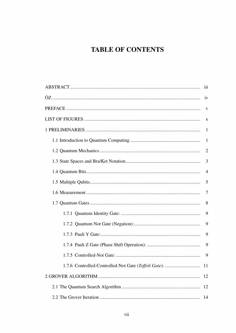
TABLE OF CONTENTS
ABSTRACT.............................................................................................................. iii
OZ ............................................................................................................................. iv
PREFACE ................................................................................................................. v
LIST OF FIGURES .................................................................................................. x
1 PRELIMINARIES ................................................................................................. 1
1.1 Introduction to Quantum Computing ........................................................... 1
1.2 Quantum Mechanics ..................................................................................... 2
1.3 State Spaces and Bra/Ket Notation............................................................... 3
1.4 Quantum Bits................................................................................................ 4
1.5 Multiple Qubits............................................................................................. 5
1.6 Measurement ................................................................................................ 7
1.7 Quantum Gates ............................................................................................. 8
1.7.1 Quantum Identity Gate: ................................................................... 9
1.7.2 Quantum Not Gate (Negation):........................................................ 9
1.7.3 Pauli Y Gate:.................................................................................... 9
1.7.4 Pauli Z Gate (Phase Shift Operation): ............................................. 9
1.7.5 Controlled-Not Gate: ....................................................................... 9
1.7.6 Controlled-Controlled-Not Gate (Toffoli Gate): .............................. 11
2 GROVER ALGORITHM ...................................................................................... 12
2.1 The Quantum Search Algorithm .................................................................. 12
2.2 The Grover Iteration ..................................................................................... 14
vii
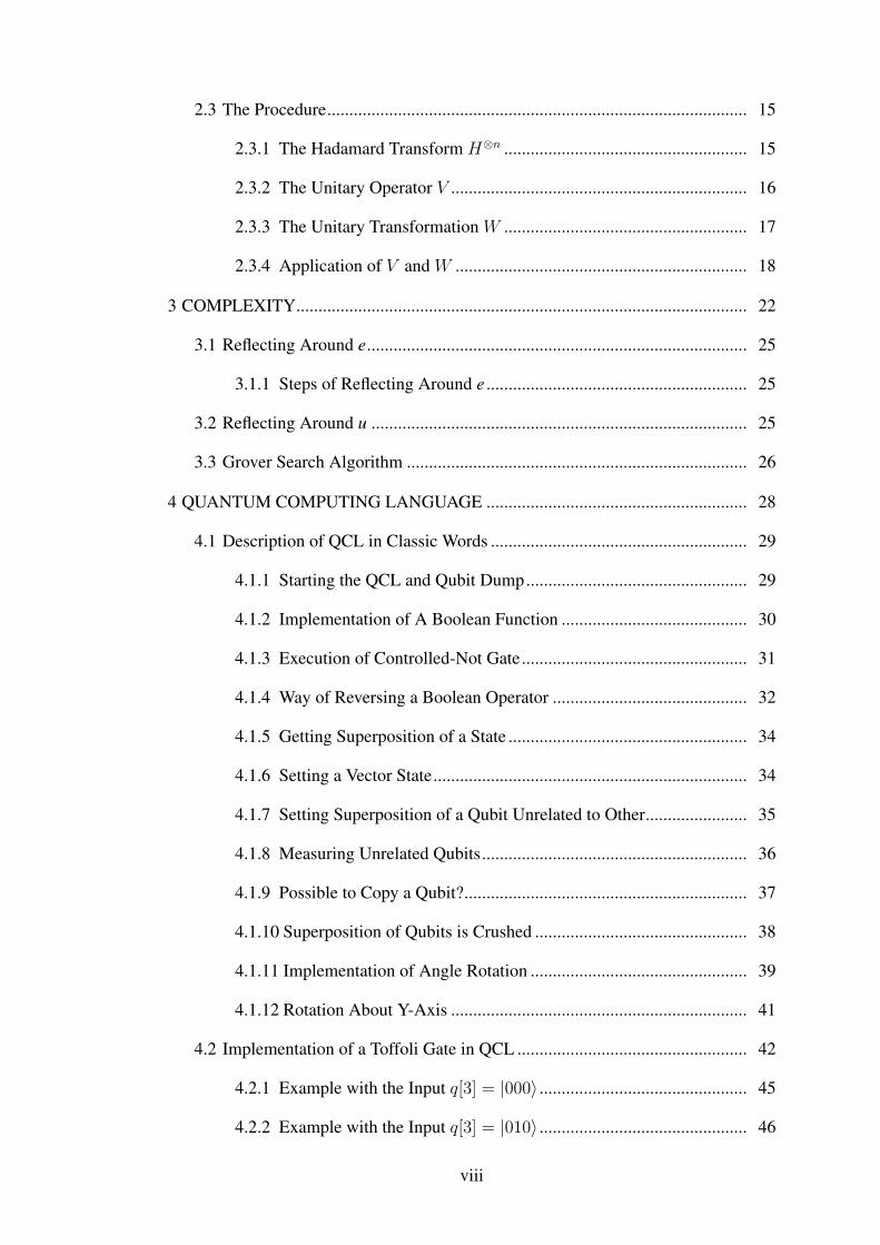
2.3 The Procedure............................................................................................... 15
2.3.1 The Hadamard Transform H⊗n ....................................................... 15
2.3.2 The Unitary Operator V ................................................................... 16
2.3.3 The Unitary Transformation W ....................................................... 17
2.3.4 Application of V and W .................................................................. 18
3 COMPLEXITY...................................................................................................... 22
3.1 Reflecting Around e...................................................................................... 25
3.1.1 Steps of Reflecting Around e ........................................................... 25
3.2 Reflecting Around u ..................................................................................... 25
3.3 Grover Search Algorithm ............................................................................. 26
4 QUANTUM COMPUTING LANGUAGE ........................................................... 28
4.1 Description of QCL in Classic Words .......................................................... 29
4.1.1 Starting the QCL and Qubit Dump.................................................. 29
4.1.2 Implementation of A Boolean Function .......................................... 30
4.1.3 Execution of Controlled-Not Gate................................................... 31
4.1.4 Way of Reversing a Boolean Operator ............................................ 32
4.1.5 Getting Superposition of a State ...................................................... 34
4.1.6 Setting a Vector State....................................................................... 34
4.1.7 Setting Superposition of a Qubit Unrelated to Other....................... 35
4.1.8 Measuring Unrelated Qubits............................................................ 36
4.1.9 Possible to Copy a Qubit?................................................................ 37
4.1.10 Superposition of Qubits is Crushed ................................................ 38
4.1.11 Implementation of Angle Rotation ................................................. 39
4.1.12 Rotation About Y-Axis ................................................................... 41
4.2 Implementation of a Toffoli Gate in QCL .................................................... 42
4.2.1 Example with the Input q[3] = |000〉 ............................................... 45
4.2.2 Example with the Input q[3] = |010〉 ............................................... 46
viii
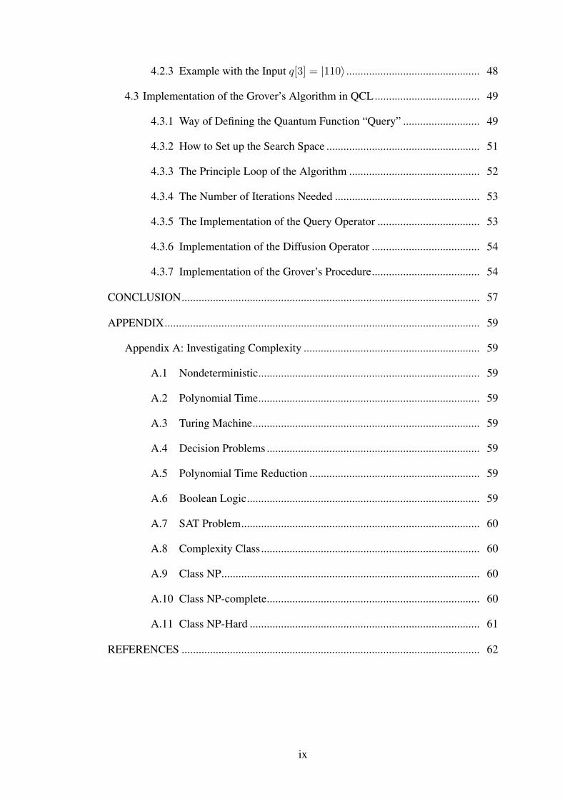
4.2.3 Example with the Input q[3] = |110〉 ............................................... 48
4.3 Implementation of the Grover’s Algorithm in QCL..................................... 49
4.3.1 Way of Defining the Quantum Function “Query” ........................... 49
4.3.2 How to Set up the Search Space ...................................................... 51
4.3.3 The Principle Loop of the Algorithm .............................................. 52
4.3.4 The Number of Iterations Needed ................................................... 53
4.3.5 The Implementation of the Query Operator .................................... 53
4.3.6 Implementation of the Diffusion Operator ...................................... 54
4.3.7 Implementation of the Grover’s Procedure...................................... 54
CONCLUSION......................................................................................................... 57
APPENDIX............................................................................................................... 59
Appendix A: Investigating Complexity .............................................................. 59
A.1 Nondeterministic.............................................................................. 59
A.2 Polynomial Time.............................................................................. 59
A.3 Turing Machine................................................................................ 59
A.4 Decision Problems ........................................................................... 59
A.5 Polynomial Time Reduction ............................................................ 59
A.6 Boolean Logic.................................................................................. 59
A.7 SAT Problem.................................................................................... 60
A.8 Complexity Class............................................................................. 60
A.9 Class NP........................................................................................... 60
A.10 Class NP-complete........................................................................... 60
A.11 Class NP-Hard ................................................................................. 61
REFERENCES ......................................................................................................... 62
ix
LIST OF FIGURES
Figure 1.1: Controlled-Not Gate...................................................................... 10
Figure 1.2: Controlled-Controlled-Not Gate (Toffoli Gate)............................. 11
Figure 1.3: Labeled Boxes ............................................................................... 11
Figure 2.1: Rotation of |φ〉 .............................................................................. 20
Figure 2.2: Rotation by 3θ ............................................................................... 21
Figure 3.1: Reflection of w .............................................................................. 24
Figure 4.1: Dumping a Qubit ........................................................................... 30
Figure 4.2: A Boolean Function in QCL ......................................................... 31
Figure 4.3: Controlled-Not Gate in QCL......................................................... 31
Figure 4.4: Reversing in QCL.......................................................................... 33
Figure 4.5: Superposition Operator Mix() ....................................................... 34
Figure 4.6: Quantum Computer with a Vector State........................................ 35
Figure 4.7: Unrelated Qubits in Superposition States...................................... 36
Figure 4.8: Measuring Unrelated Qubits ......................................................... 37
Figure 4.9: Preparing State for Copy ............................................................... 38
Figure 4.10: Measurement Disappointments ..................................................... 39
Figure 4.11: Controlled Phase Rotation............................................................. 40
Figure 4.12: Rotation About Y-Axis.................................................................. 41
Figure 4.13: Making Hadamard Using Rotation ............................................... 42
Figure 4.14: Toffoli Gate in Other Words.......................................................... 43
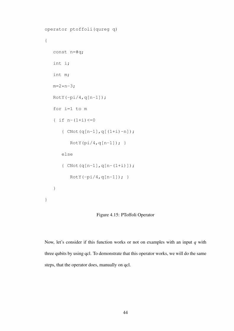
Figure 4.15: PToffoli Operator........................................................................... 44
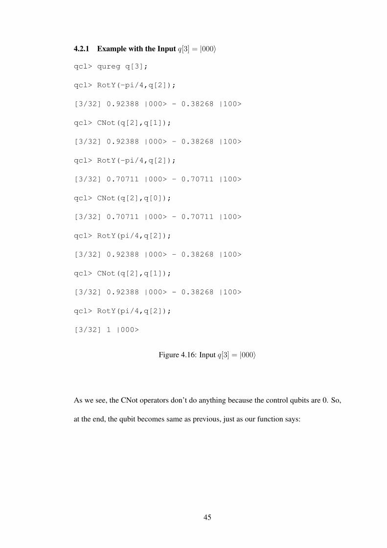
Figure 4.16: Input q[3] = |000〉.......................................................................... 45
Figure 4.17: PToffoli with q[3] = |000〉............................................................. 46
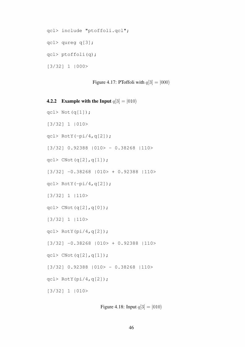
Figure 4.18: Input q[3] = |010〉.......................................................................... 46
Figure 4.19: PToffoli with q[3] = |010〉............................................................. 47
Figure 4.20: Input q[3] = |110〉.......................................................................... 48
x
Figure 4.21: PToffoli with q[3] = |110〉............................................................. 49
Figure 4.22: Function Query.............................................................................. 50
Figure 4.23: Query for Text ............................................................................... 51
Figure 4.24: Diffusion Operator ........................................................................ 54
Figure 4.25: Grover Procedure .......................................................................... 55
Figure 4.26: Application of Grover ................................................................... 56
xi
Chapter 1
PRELIMINARIES
1.1 Introduction to Quantum Computing
In the early 1980’s, Richard Feynman observed that certain quantum mechanical ef-
fects cannot be simulated efficiently on a classical computer. This observation brought
about the beliefs that general computation could be done more efficiently if it made
use of these quantum effects. Unfortunately, building computational machines that use
such quantum effects, which we called Quantum Computers, found very tricky. Even
more, no one was sure how to use the quantum effects to speed up the computation,
till 1994. In that year, Peter Shor surprised the world by describing a polynomial time
quantum algorithm for factoring integers. Then, the field of quantum computing came
into its own. This discovery prompted a flurry of activity, both among experimental-
ists trying to build quantum computers and theoreticians trying to find other quantum
algorithms. Just two years later, Lov Grover tapered with another quantum algorithm
and surprised the experimentalists again. The algorithm provided a quadratic speedup
over its classical counterpart for searching an unsorted database. Classically, the time
it takes to do certain computations can be decreased by using parallel processors. This
provides that achieving an exponential decrease in time requires an exponential in-
crease in the number of processors, and hence an exponential increase in the amount
of physical space needed. However, in quantum systems the amount of parallelism
1
increases exponentially with the size of the system. In other words, an exponential
increase in parallelism requires only a linear increase in the amount of physical space
needed. This effect is called quantum parallelism which was mentioned by David
Deutsch and Richard Jozsa in 1992.
Unexpectedly, this came along with a big handicap. While quantum system can per-
form massive parallel computation, accessing the results of the computation is strictly
restricted. Access to the results is equivalent to making a measurement which inter-
rupts the quantum state. This problem brings a situation which is even poor than the
classical one that we can only read the result of one parallel thread. Worse, because of
the measurement is probabilistic, we cannot even choose which one we get.
After all, in the past years, various people have found clever ways of addressing the
measurement problem to exploit the power of quantum parallelism. This sort of ma-
nipulation has no classical similarity, and requires non-traditional programming tech-
niques. One technique manipulates the quantum state so that a common property of all
of the output values such as the symmetry or period of a function can be read off. This
technique is used in Shor’s factorization algorithm. Another technique transforms the
quantum state to increase the probability that output of interest will be read. Such an
amplification technique is used in Grover’s search algorithm.
1.2 Quantum Mechanics
Since most of our everyday experiences are not applicable, quantum mechanical phe-
nomena are difficult to understand. Hence, we will try to give some feeling as to the
nature of quantum mechanics and some of the mathematical formalisms needed to
work with quantum mechanics to the range needed for quantum computing. Quantum
2
mechanics is a theory in the mathematical sense that it is governed by a set of axioms.
The consequences of these axioms describe the behavior of quantum systems.
1.3 State Spaces and Bra/Ket Notation
For quantum computing, we need to deal with finite quantum systems and it suffices
to consider finite dimensional complex vector spaces with inner product. We can de-
scribe the quantum state spaces and the transformations acting on them in terms of
vectors and matrices, or in the more compact bra/ket notation which was introduced
by Paul Dirac in 1939. Kets like |x〉 denote column vectors. These are typically used
to describe quantum states. The corresponding notation bra, 〈x|, denotes the conjugate
transpose of |x〉. For instance, the orthonormal basis {|0〉 , |1〉} can be expressed as{(1, 0)T , (0, 1)T
}, which is equivalent to
{(10
),(01
)}. Any complex linear combina-
tion of |0〉 and |1〉, for example a |0〉+ b |1〉, can be written as (a, b)T .
Combining 〈x| and |y〉 as in 〈x || y〉, simply written as 〈x|y〉, denotes the inner product
of the two vectors. For example, since |0〉 is a unit vector we have 〈0|0〉 = 1 , and
since |0〉 and |1〉 are orthogonal we have 〈0|1〉 = 0.
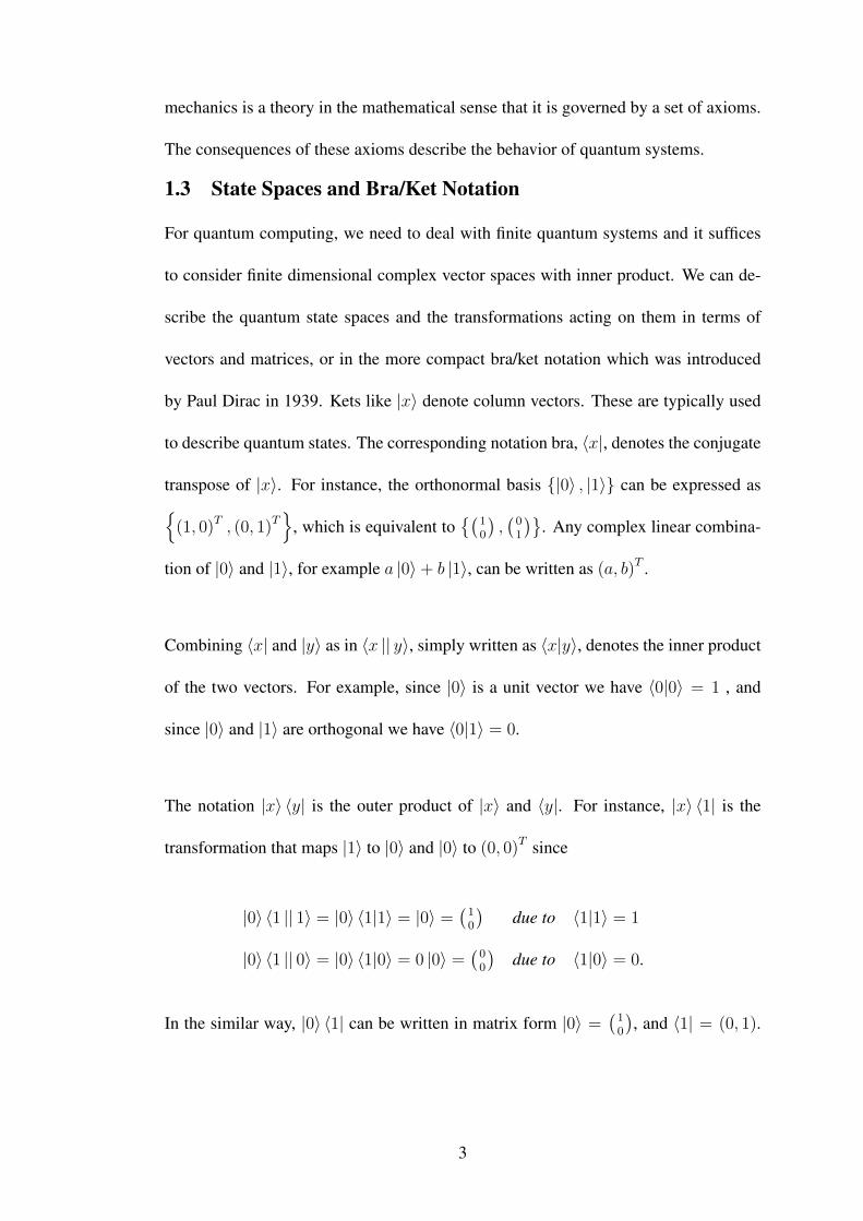
The notation |x〉 〈y| is the outer product of |x〉 and 〈y|. For instance, |x〉 〈1| is the
transformation that maps |1〉 to |0〉 and |0〉 to (0, 0)T since
|0〉 〈1 || 1〉 = |0〉 〈1|1〉 = |0〉 =(10
)due to 〈1|1〉 = 1
|0〉 〈1 || 0〉 = |0〉 〈1|0〉 = 0 |0〉 =(00
)due to 〈1|0〉 = 0.
In the similar way, |0〉 〈1| can be written in matrix form |0〉 =(10
), and 〈1| = (0, 1).
3
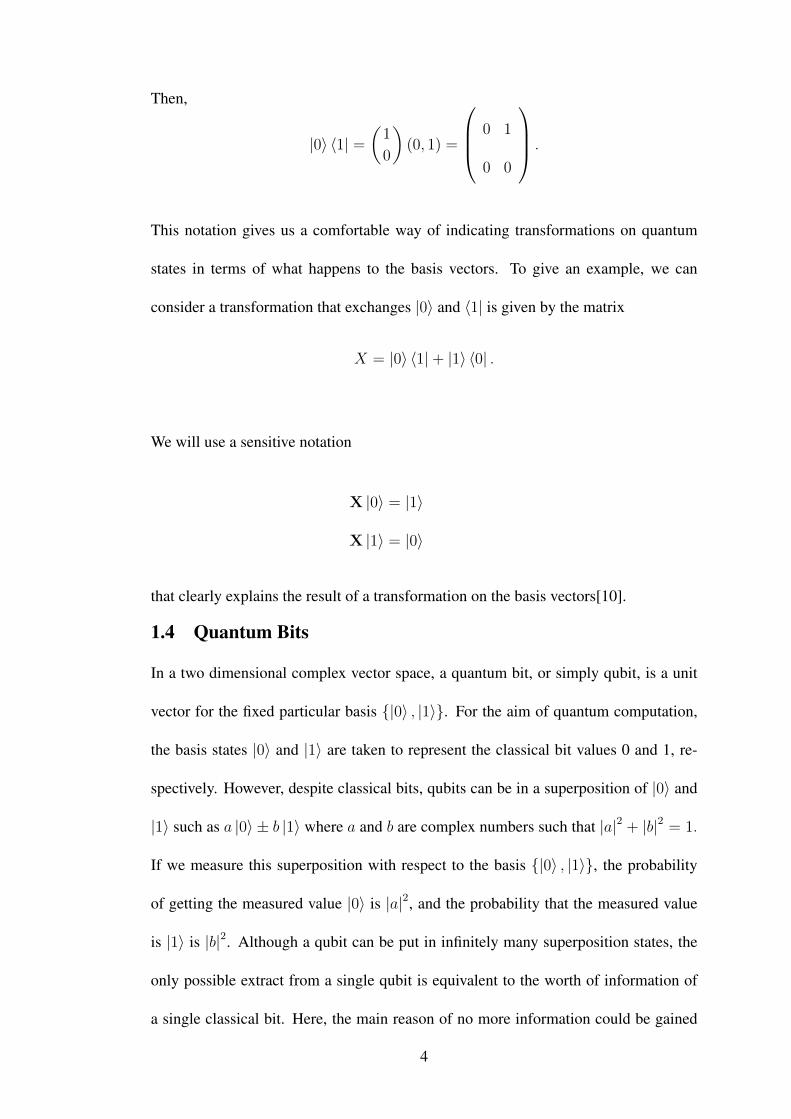
Then,
|0〉 〈1| =(
1
0
)(0, 1) =
0 1
0 0
.
This notation gives us a comfortable way of indicating transformations on quantum
states in terms of what happens to the basis vectors. To give an example, we can
consider a transformation that exchanges |0〉 and 〈1| is given by the matrix
X = |0〉 〈1|+ |1〉 〈0| .
We will use a sensitive notation
X |0〉 = |1〉
X |1〉 = |0〉
that clearly explains the result of a transformation on the basis vectors[10].
1.4 Quantum Bits
In a two dimensional complex vector space, a quantum bit, or simply qubit, is a unit
vector for the fixed particular basis {|0〉 , |1〉}. For the aim of quantum computation,
the basis states |0〉 and |1〉 are taken to represent the classical bit values 0 and 1, re-
spectively. However, despite classical bits, qubits can be in a superposition of |0〉 and
|1〉 such as a |0〉 ± b |1〉 where a and b are complex numbers such that |a|2 + |b|2 = 1.
If we measure this superposition with respect to the basis {|0〉 , |1〉}, the probability
of getting the measured value |0〉 is |a|2, and the probability that the measured value
is |1〉 is |b|2. Although a qubit can be put in infinitely many superposition states, the
only possible extract from a single qubit is equivalent to the worth of information of
a single classical bit. Here, the main reason of no more information could be gained
4
from a qubit than from a classical bit is this information can only be achieved by mea-
surement. When we measure a qubit, the measurement changes the state to one of the
basis states. Since every measurement can result in only one of two states, one of the
basis vectors associated to the given measuring device. So, there are only two possi-
ble results just like in the classical case. As measurement changes the state, it is not
possible to measure the state of a qubit in two different bases.
1.5 Multiple Qubits
The state of a qubit can be represented by a vector in the two dimensional complex
vector space spanned by |0〉 and |1〉 as we considered before. In classical physics, the
possible states of a system of n particles, such that individual states can be described by
a vector in a two dimensional vector space, form a vector space of 2n dimensions. But,
in a quantum system, a system of n qubits has a state space of 2n dimensions which is
much larger than the classical one. Here the state space is the set of normalized vectors
in this 2n dimensional space, just as the state a |0〉 + b |1〉 of a qubit is normalized so
that |a|2 + |b|2 = 1. Actually, this is the exponential growth of the state space with the
number of particles that suggests a possible exponential speed-up of computation on
quantum computers over classical ones. While individual state spaces of n particles
combine classically through the Cartesian product, quantum states combine through
the tensor product.
Instead of talking only about the tensor product, which is already explained in Ap-
pendix A before, let’s take a look on the differences of the Cartesian and the tensor
product that will be fateful to understand quantum computation.
Let V and W be 2 two-dimensional complex vector spaces with bases {v1, v2} for
5
V , and {w1, w2} for W . The Cartesian product V × W can take as its basis the
union of the bases of its component spaces {v1, v2, w1, w2}. Because dim (X × Y ) =
dim (X) + dim (Y ), easy to see that the dimension of the state space of multiple
classical particles grows linearly with the number of particles. The tensor product of
V and W has basis {v1 ⊗ w1, v1 ⊗ w2, v2 ⊗ w1, v2 ⊗ w2}. So, the state space for two
qubits, each with basis {|0〉 , |1〉}, has basis {|0〉 ⊗ |0〉 , |0〉 ⊗ |1〉 , |1〉 ⊗ |0〉 , |1〉 ⊗ |1〉}
which can also be noted as {|00〉 , |01〉 , |10〉 , |11〉}. In a more general manner, we
write |x〉 to mean |bnbn−1...b0〉 where bi are the binary digits of the number x.
A basis for a three qubit system is {|000〉 , |001〉 , |010〉 , |011〉 , |100〉 , |101〉 , |110〉 , |111〉}.
So, in general, an n qubit system has 2n basis vectors. Now, we can see the exponential
growth of the state space with the number of quantum particles. The tensor product
X ⊗ Y has dimension dim (X)× dim (Y ).
But, as it is more clear now, we can see the recycling is not possible. The state |00〉 +
|11〉 is an example of a quantum state that cannot be described in terms of the state of
each of its qubits separately. In other words, we cannot find {a1, a2, b1, b2} such that
(a1 |0〉+ b1 |1〉)⊗ (a2 |0〉+ b2 |1〉) = |00〉+ |11〉
since (a1 |0〉+ b1 |1〉)⊗ (a2 |0〉+ b2 |1〉) = a1a2 |00〉+a1b2 |01〉+b1a2 |10〉+b1b2 |11〉
and a1b2 = 0 implies that either a1a2 = 0 or b1b2 = 0. States which cannot be
decomposed in this way are called entangled states. These states represent situations
which have no classical counterpart. Besides, these are the states that provide the
exponential growth of quantum state spaces with the number of particles.
6
1.6 Measurement
The result of a measurement is probabilistic and the process of measurement changes
the state to that measured. Here is an example of measurement in a two qubit system.
Any two qubit state can be expressed as a |00〉+ b |01〉+ c |10〉+ d |11〉, where a, b, c,
and d are complex numbers such that
|a|2 + |b|2 + |c|2 + |d|2 = 1.
Suppose we wish to measure the first qubit with respect to the standard basis {|0〉 , |1〉}.
For convenience, we will rewrite the state a |00〉+ b |01〉+ c |10〉+ d |11〉.
a |00〉+ b |01〉+ c |10〉+ d |11〉 = |0〉 ⊗ (a |0〉+ b |1〉) + |1〉 ⊗ (c |0〉+ d |1〉)
= v |0〉 ⊗(
a
v |0〉+
b
v |1〉
)+ w |1〉 ⊗
(c
w |0〉+
d
w |1〉
)
For v =√|a|2 + |b|2 and w =
√|c|2 + |d|2 the vectors a/v |0〉+b/v |1〉 and c/w |0〉+
d/w |1〉 are of unit length. Once we write the state as above which is a tensor product
of the bit being measured and a second vector of unit length, the probabilistic result
of a measurement is easy to read off. Measurement of the first bit will return |0〉 with
probability v2 = |a|2 + |b|2 projecting the state to |0〉 ⊗ (a/v |0〉+ b/u |1〉) or return
|1〉 with probability w = |c|2 + |d|2 projecting the state to |1〉 ⊗ (c/w |0〉+ d/w |1〉).
As |0〉 ⊗ (a/v |0〉+ b/u |1〉) and |1〉 ⊗ (c/w |0〉+ d/w |1〉) are both unit vectors, no
scaling is necessary. In the same manner, measuring the second bit works similarly.
Any quantum state can be written as the sum of two vectors, one in each of the sub-
spaces. A measurement of k qubits in the standard basis has 2k possible outcomes.
Measuring k qubits of an n-qubit system splits of the 2n-dimensional state spaceH into
7
a Cartesian product of orthogonal subspaces S1, S2, ..., S2k withH = S1×S2×...×S2k ,
such that the value of the k qubits being measured is mi, and the state after measure-
ment is in space Si for some i. The Si is chosen randomly with probability the square
of the amplitude of the component of ψ in Si, and projects the state into that compo-
nent, scaling to give length 1. In the same manner, the probability that the result of the
measurement to be a given value is the sum of the squares of the absolute values of the
amplitudes of all basis vectors compatible with that value of measurement.
The way of the measurement brings out some other ideas about entangled particles.
Particles are not entangled if the measurement of one has no effect on the other. For
example, the state 1√2
(|00〉+ |11〉) is entangled. Because the probability of the mea-
surement of the first bit to be |0〉 is 12, if the second bit has not been measured. However,
if the second bit had also been measured, the probability of the measurement of the first
bit to be |0〉 would be either 1 or 0 depending on whether the second bit was measured
as |0〉 or |1〉 respectively. This why, the possible result of measuring the first bit is
changed by a measurement of the second bit. Unlikely, the state 1√2
(|00〉+ |01〉) is
not entangled. Because 1√2
(|00〉+ |11〉) = |0〉 ⊗ 1√2
(|0〉+ |1〉), any measurement of
the first bit will return |0〉 regardless of whether the second bit was measured or not.
Likewise, the second bit has 50% chance of being measured as |0〉 without considera-
tion whether the first bit was measured.
1.7 Quantum Gates
Any linear transformation on a complex vector space can be described by a matrix.
Let M † denote the conjugate transpose of the matrix M . A matrix M is unitary if
MM † = I . In other words, we say M is a unitary transformation. The most important
property of it is that any unitary transformation is reversible. Here is the explanation
8
of some useful simple, single-qubit, quantum state transformations, each with a little
example in addition:
1.7.1 Quantum Identity Gate:
I =
1 0
0 1
|0〉 → I → |0〉
|1〉 → I → |1〉α |0〉+ β |1〉 → I → α |0〉+ β |1〉
1.7.2 Quantum Not Gate (Negation):
X =
0 1
1 0
|0〉 → X → |1〉
|1〉 → X → |0〉α |0〉+ β |1〉 → X → α |1〉+ β |0〉
1.7.3 Pauli Y Gate:
Y =
0 1
−1 0
|0〉 → Y → −|1〉
|1〉 → Y → |0〉α |0〉+ β |1〉 → Y → i (α |1〉 − β |0〉)
1.7.4 Pauli Z Gate (Phase Shift Operation):
Z =
1 0
0 −1
|0〉 → Z → |0〉
|1〉 → Z → −|1〉α |0〉+ β |1〉 → Z → α |0〉 − β |1〉
It can be easily verified that these gates are unitary. For instance
Y Y † =
0 1
−1 0
0 −1
1 0
= I.
1.7.5 Controlled-Not Gate:
The controlled-not gate CNOT works in a way that it changes the second bit if the first
bit is 1, and leaves this bit unchanged otherwise. In order to represent transformations
9
of this space in matrix notation we need to choose an isomorphism between this space
and the space of complex four tuples. Such an isomorphism associates basis |00〉, |01〉,
|10〉, and |11〉 to the standard 4-tuple basis (1, 0, 0, 0)T , (0, 1, 0, 0)T , (0, 0, 1, 0)T , and
(0, 0, 0, 1)T respectively. So, we have CNOT with the representations
CNOT:
|00〉 → |00〉
|01〉 → |01〉
|10〉 → |11〉
|11〉 → |10〉
1 0 0 0
0 1 0 0
0 0 0 1
0 0 1 0
.
The transformation CNOT is unitary since CNOT † = CNOT and CNOTCNOT =
I . In addition, the CNOT gate cannot be decomposed into a tensor product of two
single-bit transformations.
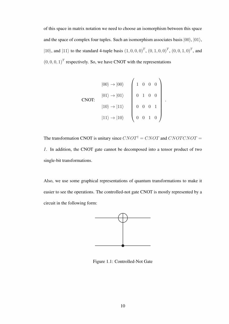
Also, we use some graphical representations of quantum transformations to make it
easier to see the operations. The controlled-not gate CNOT is mostly represented by a
circuit in the following form:
Figure 1.1: Controlled-Not Gate
10
Here, the black point indicates the control bit, and the solid circle indicates the target
bit, which is toggled when the control bit is 0.
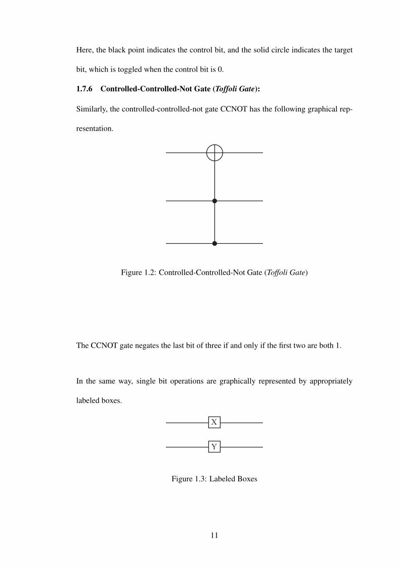
1.7.6 Controlled-Controlled-Not Gate (Toffoli Gate):
Similarly, the controlled-controlled-not gate CCNOT has the following graphical rep-
resentation.
Figure 1.2: Controlled-Controlled-Not Gate (Toffoli Gate)
The CCNOT gate negates the last bit of three if and only if the first two are both 1.
In the same way, single bit operations are graphically represented by appropriately
labeled boxes.
X
Y
Figure 1.3: Labeled Boxes
11
Chapter 2
GROVER ALGORITHM
2.1 The Quantum Search Algorithm
In models of classical computation, searching through every item is optimal. In other
words, searching an unsorted database cannot be done in less than linear time. Grover’s
algorithm clarifies that searching can be done faster than this in the quantum model.
Even more, it is asymptotically the fastest possible algorithm for searching an unsorted
database in the quantum model with the time complexity O(N1/2
)[1]. Unfortunately,
it provides only a quadratic speedup, while other quantum algorithms provide expo-
nential speedup over their classical counterparts. But still, even quadratic speedup is
very substantial when N is large. The quantum search algorithm reaches to the solu-
tion with a generic search applied to a very wide range of problems. Like many other
quantum algorithms, it is also probabilistic which gives the correct answer with the
high probability. But yet, we can decrease the probability of failure by repeating the
algorithm. In order to make it clear, let’s consider an example. Suppose we know that
exactly one n-bit integer satisfies a certain condition, and have a black-boxed subrou-
tine that acts on the N = 2n different n-bit integers. It outputs 1 if the integer satisfies
the condition, otherwise 0. Without any other information, we should find the special
integer. With a classical computer, we can do no better than to apply the subroutine
repeatedly to different random numbers till it hits on the special one. Certainly, the
12
probability of finding the special number increases in every time we apply the subrou-
tine. If we apply it to M different integers, the probability of finding the special number
becomes M/N . Then, for instance, we should test 12N different integers to have a 50%
chance of success. On the other hand, if we have a quantum computer with a subrou-
tine that performs such a test for a very large N, we can find the special integer with a
probability very close to 1. Even more, using a method to find the special integer calls
the subroutine no greater than (π/4)√N number of times.
We can consider this subroutine in various ways. It might perform a mathematical
calculation to determine whether the input integer is the special one. Let’s consider it
on an example. Suppose an odd number p can be expressed as the sum of two squares,
m2 + n2. Since one of m or n must be even and the other odd, p must be of the form
4k + 1. This is actually an elementary theorem of the number theory: If p is a prime
number of the form 4k + 1, then it can always be expressed as the sum of two squares,
and in exactly one way. For instance, 5 = 4+1, 13 = 9+4, 17 = 16+1, 29 = 25+4,
37 = 36 + 1, 41 = 25 + 16, 53 = 49 + 4, 61 = 36 + 25, etc. Given such a prime
p, the simple-minded way to and the two squares is to take randomly selected integers
x where 1 ≤ x ≤ N , with N =⌊√
p/2⌋
. And, repeat this till we and such an x
for which√p− x2 = a, where a is an integer. Now, imagine p is of the order of a
trillion, then following the same procedure we would have to calculate√p− x2 = a
for nearly a million x to get a better than even chance of succeeding. Fortunately,
using the quantum search algorithm with a suitably programmed quantum computer,
we could find the two squares with a probability of success extremely close to 1 by
calling the quantum subroutine, which evaluated√p− x2, only fewer than a thousand
times.
13
This very general capability of quantum computers was discovered by Lov Grover,
and goes under the name of Grover’s search algorithm. Shor’s period-finding algo-
rithm and Grover’s search algorithm, together with their various modifications and
extensions, constitute the two masterpieces of the quantum - computational software.
2.2 The Grover Iteration
Grover’s algorithm actually makes operations to answer a “Yes or No” question, if the
input is a solution for the search problem. In other words, mathematically, it is just a
boolean function. By defining the variables N, the size of the search elements, x, the
n-bit integer input, and a, the solution of the search problem, we can write down this
function as:
f(x) =
0 if x 6= a
1 if x = a
(2.1)
Despite the simplicity, of course the magic is here behind the computing of this prob-
lem. Grover, discovered a way for the caseN = 2n in the sense of quantum computing,
which is strictly better than the classical one. Declared a unitary operator
Uf (|x〉n |y〉1) = |x〉n |y ⊕ f (x)〉1 (2.2)
where |x〉 is the index register of the input x, ⊕ denotes the addition modulo 2, and |y〉
(oracle qubit) is a single qubit which is flipped if f(x) = 1. This operator also called
as the Oracle Operator in some books. The aim here is to check if the single qubit
|y〉 is flipped or not. In this way, it is useful to take the |y〉 in the initial state H |1〉 =
(|0〉−|1〉)/√
2. If |y〉 is flipped, then x is the solution of the search problem, i.e. x = a,
and the state becomes − |x〉 (|0〉 − |1〉)/√
2 . Otherwise, |y〉 stays unchanged. We can
14
write this operation as:
Uf (|x〉n |y〉1) = Uf (|x〉nH |1〉) = (−1)f(x) |x〉 ( |0〉 − |1〉√2
) (2.3)
In the classical way, we could do no better than to try each of the N = 2n possible
inputs to check if the output register is flipped. Though by using Grover’s algorithm,
when the N is large, we can get the same answer only by performing the search sub-
routine no more than√N = 2n/2 times (or more precisely (π/4)
√N ).
2.3 The Procedure
Now, we can define an algorithm to show that how the quantum search procedure
works. Let’s first define the procedure, then we can discuss it step by step.
1. Apply the Hadamard transform H⊗n.
2. Apply the unitary operator V .
3. Apply the Hadamard transform H⊗n.
4. Apply the unitary transformation W .
5. Apply the Hadamard transform H⊗n.
2.3.1 The Hadamard Transform H⊗n
The algorithm starts with the computer in the state |0〉⊗n. Next, we will use the
Hadamard transform[4],
H |1〉 =1√2
(|0〉 − |1〉) , (2.4)
on the n-Qubit input register to put the computer in the equal superposition state
|φ〉 = H⊗n |0〉n =1√N
N−1∑x=0
|x〉n =1√2n
2n−1∑x=0
|x〉n . (2.5)
15
2.3.2 The Unitary Operator V
The action of Uf is then to multiply the (n+ 1)-Qubit state by -1 if and only if x = a:
Uf (|x〉 ⊗H |1〉) = (−1)f(x) |x〉 ⊗H |1〉 . (2.6)
Obviously, Uf does not have any effect on the single qubit which is H |1〉 in this case.
Then, we can define an n-Qubit unitary transformation V on Uf , which is also linear
as Uf is.
V |x〉 = (−1)f(x) |x〉 =
|x〉 , x 6= a
− |a〉 , x = a
(2.7)
Necessity use of the unitary operator V instead of Uf of course deserves an explana-
tion here. V changes the sign of the component of the general superposition |Ψ〉 =∑x |x〉 〈x |Ψ〉 of the computational basis state with |a〉, and leaves the orthogonal
component to |a〉 unchanged:
V |Ψ〉 = |Ψ〉 − 2 |a〉 〈a |Ψ〉 (2.8)
Which can be simply implemented as
V = 1− 2 |a〉 〈a| . (2.9)
Here, |a〉 〈a| denotes the projection operator (which has been described in the
16
Appendix A) on the state |a〉. As we could notice clearly, the unitary transformation
Uf acts as nothing but the identity operator on the output register. The output register
starts in the H |1〉 state unentangled with the input register. In addition, Uf
determines the output register particularly which makes the output register remain
unentangled with the input register. Then, for instance, we can write the equation
(2.9) again in the terms of Uf as:
Uf (|Ψ〉 ⊗H |1〉) = (|Ψ〉 − 2 |a〉 〈a |Ψ〉)⊗H |1〉 (2.10)
So, obviously, we can use V instead of using Uf to implement things in a more
simple way.
2.3.3 The Unitary Transformation W
We can define a second n-Qubit unitary W which is going to act on the input register
with a similar manner with V. But this time, it’ll be in a fixed form which does not
depend on a. We will use it to simply denote the component of any state along the
standard state |φ〉, which we have defined before in (2.5), changing the sign of its
component orthogonal to |φ〉:
W = 2 |φ〉 〈φ| − 1 (2.11)
Again, |φ〉 〈φ| denotes the projection operator on the state|φ〉. Unfortunately, the way
to build W out of 1 and 2 Qubit unitary gates is not that obvious, and will be
mentioned in another section.
17
2.3.4 Application of V and W
As we have constructed the unitary operators V and W successfully, now we can use
them on the initial state |φ〉. To see what we get by repeatedly applying WV to the |φ〉,
remember that both V and W acting on either |φ〉 or |a〉 results in linear combinations
of these two states. Since 〈a |φ〉 = 〈φ |a〉 = 1/2n/2 is true for any value of a, the linear
combinations have real coefficients such that
V |a〉 = − |a〉 , V |φ〉 = |φ〉 − 22n/2 |a〉
W |φ〉 = − |φ〉 , W |a〉 = 22n/2 |φ〉 − |a〉
(2.12)
Let’s start with the state |φ〉 and suppose any sequence of V and W act successively,
then the resulting states will always remain in the two - dimensional plane spanned by
real linear combinations of |φ〉 and |a〉. Consequently, finding the result of repeated
applications of WV to the initial state |φ〉 lessens to an exercise in plane geometry.
We continue with the form (2.3) of |φ〉. If we consider|φ〉 and |a〉 as vectors in the
plane of their real linear combinations, they are very nearly perpendicular because of
the cosine of the angle γ between them is given by
cos γ = 〈a |φ〉 = 2−n/2 = 1/√N (2.13)
which gets smaller when N gets larger. Appropriately, we can define |a⊥〉 to be the
normalized real linear combination of |φ〉 and |a〉 that is strictly orthogonal to |a〉 and
makes the small angle θ = π/2− γ with |φ〉, as illustrated in 2.1 and 2.2. Since
18
sin θ = cos γ = 2−n/2 = 1/√N (2.14)
θ is very accurately give by
θ ≈ 2−n/2 (2.15)
when√N is large.
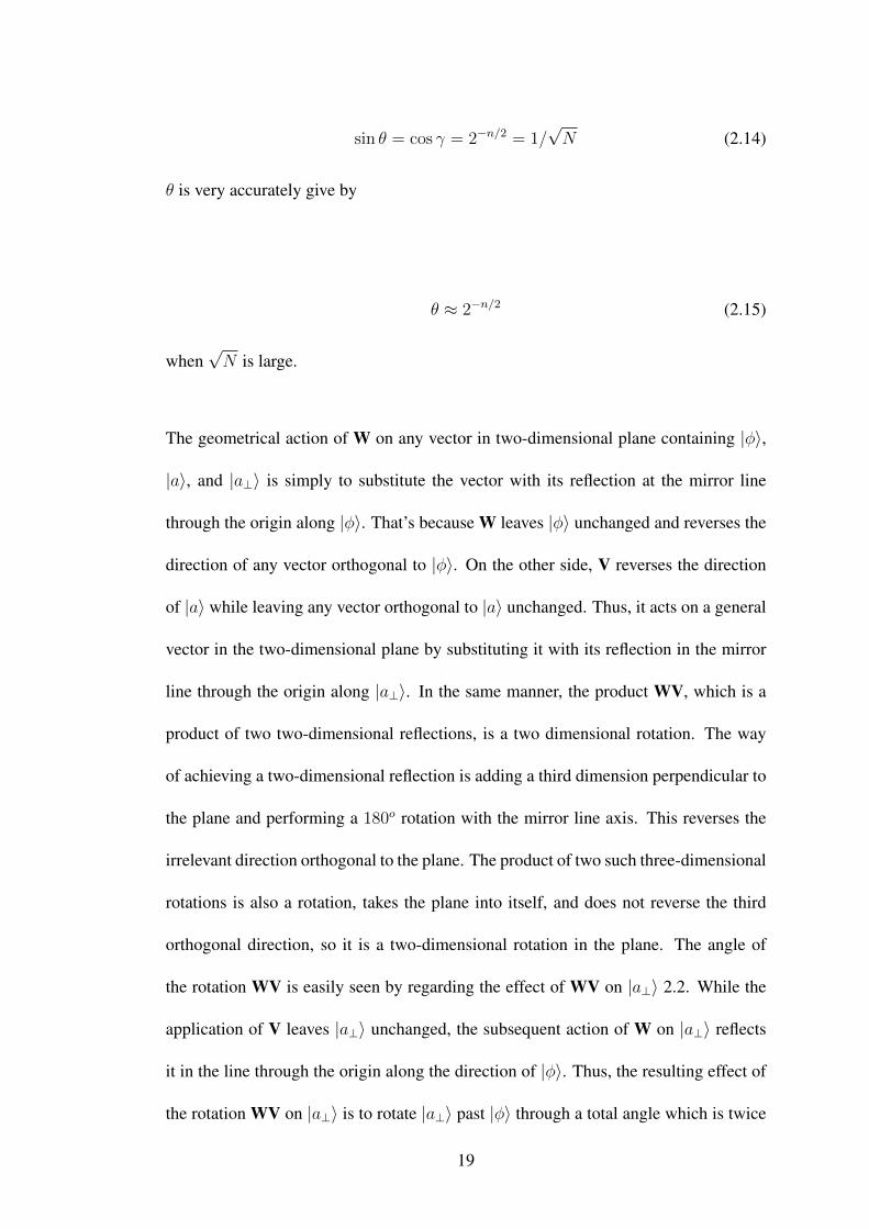
The geometrical action of W on any vector in two-dimensional plane containing |φ〉,
|a〉, and |a⊥〉 is simply to substitute the vector with its reflection at the mirror line
through the origin along |φ〉. That’s because W leaves |φ〉 unchanged and reverses the
direction of any vector orthogonal to |φ〉. On the other side, V reverses the direction
of |a〉 while leaving any vector orthogonal to |a〉 unchanged. Thus, it acts on a general
vector in the two-dimensional plane by substituting it with its reflection in the mirror
line through the origin along |a⊥〉. In the same manner, the product WV, which is a
product of two two-dimensional reflections, is a two dimensional rotation. The way
of achieving a two-dimensional reflection is adding a third dimension perpendicular to
the plane and performing a 180o rotation with the mirror line axis. This reverses the
irrelevant direction orthogonal to the plane. The product of two such three-dimensional
rotations is also a rotation, takes the plane into itself, and does not reverse the third
orthogonal direction, so it is a two-dimensional rotation in the plane. The angle of
the rotation WV is easily seen by regarding the effect of WV on |a⊥〉 2.2. While the
application of V leaves |a⊥〉 unchanged, the subsequent action of W on |a⊥〉 reflects
it in the line through the origin along the direction of |φ〉. Thus, the resulting effect of
the rotation WV on |a⊥〉 is to rotate |a⊥〉 past |φ〉 through a total angle which is twice
19
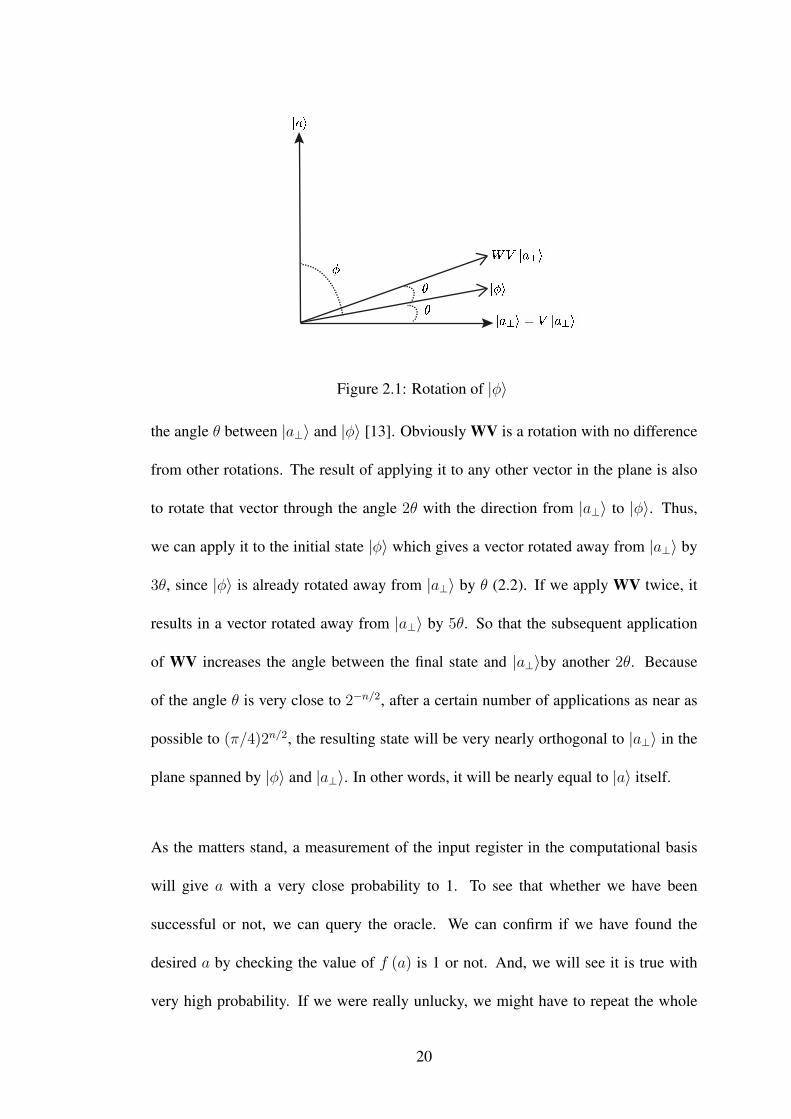
Figure 2.1: Rotation of |φ〉
the angle θ between |a⊥〉 and |φ〉 [13]. Obviously WV is a rotation with no difference
from other rotations. The result of applying it to any other vector in the plane is also
to rotate that vector through the angle 2θ with the direction from |a⊥〉 to |φ〉. Thus,
we can apply it to the initial state |φ〉 which gives a vector rotated away from |a⊥〉 by
3θ, since |φ〉 is already rotated away from |a⊥〉 by θ (2.2). If we apply WV twice, it
results in a vector rotated away from |a⊥〉 by 5θ. So that the subsequent application
of WV increases the angle between the final state and |a⊥〉by another 2θ. Because
of the angle θ is very close to 2−n/2, after a certain number of applications as near as
possible to (π/4)2n/2, the resulting state will be very nearly orthogonal to |a⊥〉 in the
plane spanned by |φ〉 and |a⊥〉. In other words, it will be nearly equal to |a〉 itself.
As the matters stand, a measurement of the input register in the computational basis
will give a with a very close probability to 1. To see that whether we have been
successful or not, we can query the oracle. We can confirm if we have found the
desired a by checking the value of f (a) is 1 or not. And, we will see it is true with
very high probability. If we were really unlucky, we might have to repeat the whole
20
procedure a few more times to get the right answer.
Figure 2.2: Rotation by 3θ
21
Chapter 3
COMPLEXITY
While talking about one of the most basic and quite useful algorithm of quantum com-
puters, of course we should discuss about the complexity of this algorithm. At the rest,
I have used a lot of terms belong to the complexity theory. For any unknown notation
or name, you can check the Appendix A.
Let’s begin with a NP-complete problem SAT of finding; given n-variable Boolean for-
mula ϕ, whether there is an assignment a ∈ {0, 1}n such that ϕ (a) = 1. Customary,
we do not know how to solve this problem better than the trivial poly(n) 2n-time algo-
rithm by using “classical” deterministic or probabilistic TM’s. But, Grover’s algorithm
solves SAT in poly(n) 2n/2-time on a quantum computer. Even if it is away of showing
that NP ⊆ BQP , this is still a significant improvement over the classical case. On the
other hand, Grover’s algorithm actually solves an even more general problem, namely,
satisfiability of a circuit with n inputs[12].
Theorem 1. (Grover’s Algorithm): There is a quantum algorithm that given as input
every polynomial-time computable function f : {0, 1}n → {0, 1} (i.e., represented
as a circuit computing f) finds in poly(n)2n/2 time a string “a” such that f (a) = 1 (if
such a string exists).
22
It is best to describe Grover’s algorithm geometrically. Assume that the function f has
a single satisfying assignment a. Consider an n-qubit register, and let u be the uniform
state vector of this register, which means
u =1
2n/2
∑x
|x〉 where x ∈ {0, 1}n .
In this way, the angle θ between u and the basis state |a〉 is equal to the inverse cosine
of their inner product
〈u, |a〉〉 =1
2n/2.
Because of this inner product is a positive number,
cos−1 (〈u, |a〉〉) = cos−1(
1
2n/2
)= θ <
π
2= 90◦ since
1
2n/2> 0.
Hence, we denote it by
π
2− θ where sinθ =
1
2n/2.
Thus, by using the inequality θ ≥ sinθ for every θ > 0, we get
θ ≥ 2−n/2.
At the beginning, the algorithm is in the state u, and at each step it gets closer to the
state |a〉. If its current state makes an angle π2− α with |a〉, then at the end of the step
it makes an angle π2− α − 2θ. Therefore, it will get to a state v whose inner product
with |a〉 is larger than 12
in
O
(1
θ
)= O
(2n/2
)steps. This implies that a measurement of the register will yield a with probability at
least 14.
23
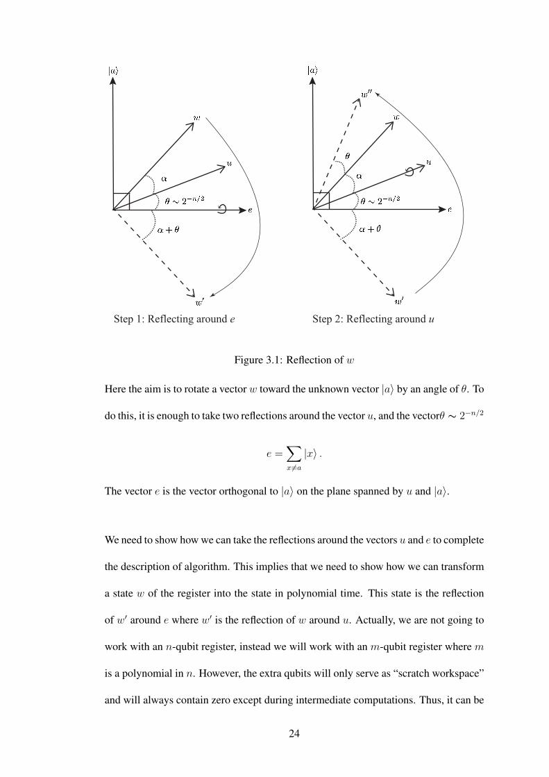
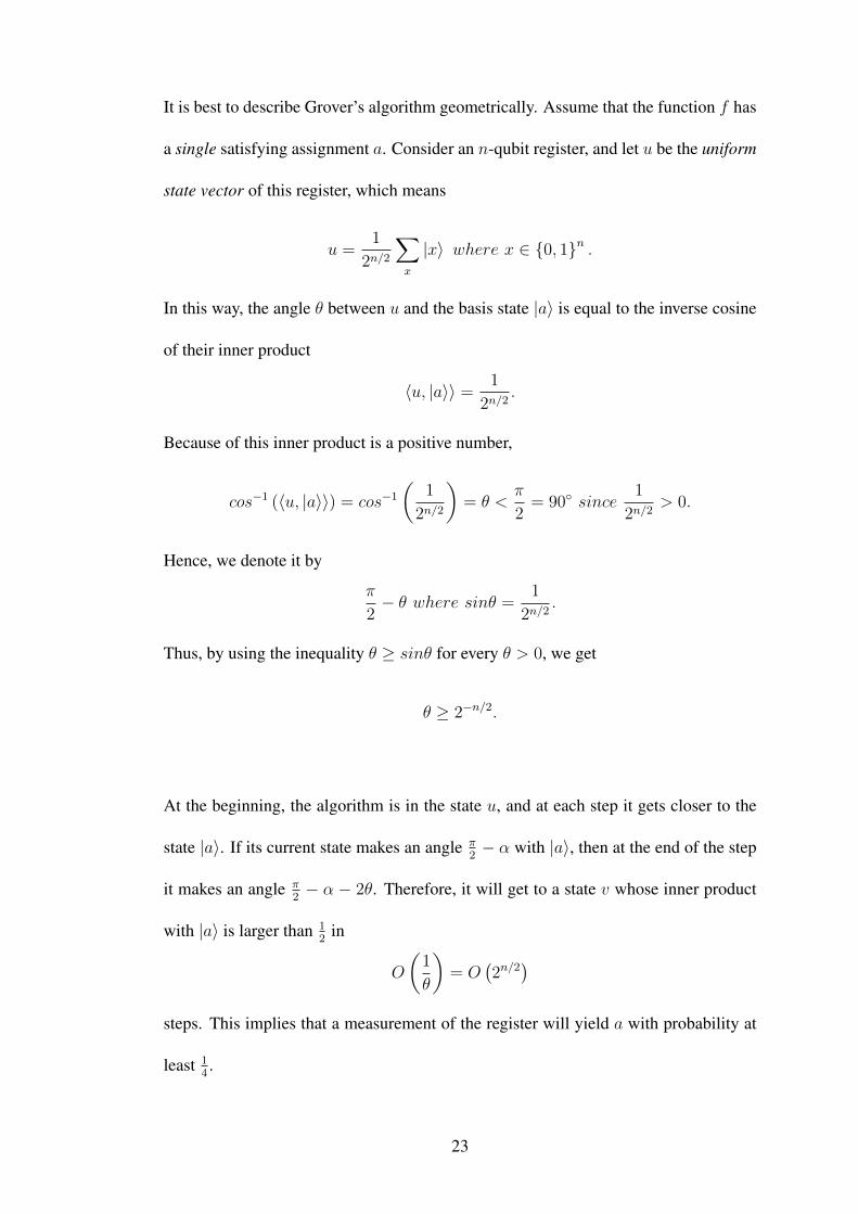
Step 1: Reflecting around e Step 2: Reflecting around u
Figure 3.1: Reflection of w
Here the aim is to rotate a vector w toward the unknown vector |a〉 by an angle of θ. To
do this, it is enough to take two reflections around the vector u, and the vectorθ ∼ 2−n/2
e =∑x 6=a
|x〉 .
The vector e is the vector orthogonal to |a〉 on the plane spanned by u and |a〉.
We need to show how we can take the reflections around the vectors u and e to complete
the description of algorithm. This implies that we need to show how we can transform
a state w of the register into the state in polynomial time. This state is the reflection
of w′ around e where w′ is the reflection of w around u. Actually, we are not going to
work with an n-qubit register, instead we will work with an m-qubit register where m
is a polynomial in n. However, the extra qubits will only serve as “scratch workspace”
and will always contain zero except during intermediate computations. Thus, it can be
24
accepted to ignore these.
3.1 Reflecting Around e
To reflect a vector w around a vector v, we indicate w as αv+ v⊥ and output αv− v⊥.
Note that v⊥ is orthogonal to v. Therefore, the reflection of w around e is equal to
∑x 6=a
wx |x〉 − wa |a〉 .
Unexpectedly, it is actually easy to represent this transformation.
3.1.1 Steps of Reflecting Around e
1. Because of f is computable in polynomial time, we can compute the transfor-
mation
|xσ〉 → |x (σ ⊕ f (x))〉
in polynomial time (This is actually same with the operator Uf that we have
defined before in 2.2). This transformation implies |x0〉 → |x0〉 for all x 6= a
and |a0〉 → |a1〉.
2. Follows that, we apply the Pauli-Z gate (1.7.4) on the qubit σ, which maps |0〉 to
|0〉 and |1〉 to − |1〉. It infers |x0〉 → |x0〉 for all x 6= a, and |a1〉 → − |a1〉.
3. After that, we apply the transformation we have used in step 1 again. This refers
|x0〉 → |x0〉 for all x 6= a and − |a1〉 → − |a0〉.
Consequently, the vector |α0〉 is mapped to itself for all x 6= a, yet |a0〉 is mapped to
− |a0〉. Ignoring the last qubit, this is exactly a reflection around |a〉.
3.2 Reflecting Around u
Instead of directly reflecting around u, we follow a different way to make this process
easier. Firstly, we apply the Hadamard operation to each qubit which maps u to |0〉.
25
Then, we make the reflection this time around |0〉. To do this, we can use the same
way as reflecting around |a〉, but this time instead of the function f using a function
g : {0, 1}n → {0, 1} which outputs 1 if and only if its input is all 0s. At last, we apply
the Hadamard operation again, mapping |0〉 back to u.
In the gleam of these operations, we can take a vector in the plane spanned by |a〉
and u, and rotate it 2θ radians closer to |a〉. Hence, if we start with the vector u, we
will only need to repeat them O (1/θ) = O(2n/2
)times to obtain a vector that, when
measured, yields |a〉 with constant probability.
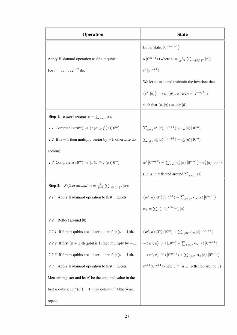
3.3 Grover Search Algorithm
Eventually, let’s try to gather all of the process into one piece.
Target: Given a polynomial - time computable f : {0, 1}n → {0, 1} with a unique
a ∈{0, 1}n such that f (a) = 1, find a.
Quantum register: We use an (n+ 1 +m)-qubit register, where m is large enough
so we can compute the transformation |xσ0m〉 → |x (σ ⊕ f (x)) 0m〉.
26
Operation State
Initial state:∣∣0n+m+1
⟩Apply Hadamard operation to first n qubits. u
∣∣0m+1⟩
(where u = 12n/2
∑x∈{0,1}n |x〉)
For i = 1, . . . , 2n/2 do: vi∣∣0m+1
⟩We let v1 = u and maintain the invariant that
⟨vi, |a〉
⟩= sin (iθ), where θ ∼ 2−n/2 is
such that 〈u, |a〉〉 = sin (θ)
Step 1: Reflect around e =∑
x 6=a |x〉:
1.1 Compute |xσ0m〉 → |x (σ ⊕ f (x)) 0m〉∑
x 6=a vix |x〉
∣∣0m+1⟩+ via |a〉 |10m〉
1.2 If α = 1 then multiply vector by −1, otherwise do
nothing.
∑x 6=a v
ix |x〉
∣∣0m+1⟩− via |a〉 |10m〉
1.3 Compute |xσ0m〉 → |x (σ ⊕ f (x)) 0m〉 wi∣∣0m+1
⟩=∑
x 6=a vix |x〉
∣∣0m+1⟩−via |a〉 |00m〉
(wi is vi reflected around∑
x 6=a |x〉)
Step 2: Reflect around u = 12n/2
∑x∈{0,1}n |x〉:
2.1 Apply Hadamard operation to first n qubits.⟨wi, u
⟩|0n〉
∣∣0m+1⟩+∑
x 6=0n αx |x〉∣∣0m+1
⟩αx =
∑z (−1)
x�zwi
z |z〉
2.2 Reflect around |0〉:
2.2.1 If first n-qubits are all zero, then flip (n+ 1)th.⟨wi, u
⟩|0n〉 |10m〉+
∑x 6=0n αx |x〉
∣∣0m+1⟩
2.2.2 If first (n+ 1)th qubit is 1, then multiply by −1. −⟨wi, u
⟩|0n〉 |10m〉+
∑x6=0n αx |x〉
∣∣0m+1⟩
2.2.3 If first n-qubits are all zero, then flip (n+ 1)th. −⟨wi, u
⟩|0n〉
∣∣0m+1⟩+∑
x 6=0n αx |x〉∣∣0m+1
⟩2.3 Apply Hadamard operation to first n qubits vi+1
∣∣0m+1⟩
(here vi+1 is wi reflected around u)
Measure register and let a′ be the obtained value in the
first n qubits. If f (a′) = 1, then output a′. Otherwise,
repeat.
27
Chapter 4
QUANTUM COMPUTING LANGUAGE
Past years induced to separate many common concepts of classical computer science
from theoretical physics. However, the quantum computer science was not that lucky
enough. Even now, quantum computing is widely considered as a special discipline
within the very wide field of theoretical physics. This slow adaption of quantum com-
puting by the computer science community was mainly caused by the confusing variety
of formalisms, like gates, operators, matrices, Dirac notation, and so on. These, in fact,
have no similarity with classical programming languages, or with physical terminology
in most of the available literature.
One of the best options to fill this breach is the Quantum Computation Language
(QCL). This language is implemented by Bernhard mer in 1998 with his master thesis
in the Technical University of Vienna. It is a high level and architecture independent
programming language for quantum computers . Syntax of it is established by deduc-
tion of classical programming languages like C or Pascal. It will be very useful of
course to implement and simulate the quantum algorithms including classical compo-
nents in one consistent formalism.
Simulating a quantum computer on a classical computer is a big problem. The amount
28
of quantum memory under simulation increases exponentially with the resources re-
quired. This, distressfully, points that simulating a quantum computer with even a few
dozen qubits is beyond the capability of any computer made today. Even this language
simulates very small quantum computers, it is still powerful enough to demonstrate the
concept behind some useful quantum algorithms.
It is most inevitable that the first quantum computers will probably consist of some
exotic hardware at the core which stores and manipulates the quantum state machine
just like happened by the supercomputers of last years. Inclosing this will be the hard-
ware that supports it and presents the user with a reasonable programming environ-
ment. This language makes it available to simulate such an environment by providing
a classical program structure with quantum data types and special functions to perform
operations on them.
4.1 Description of QCL in Classic Words
To describe this very powerful language, let’s start with demonstrating some familiar
operations of classical computing languages with QCL.
4.1.1 Starting the QCL and Qubit Dump
To make the qubits implemented as Dirac notation, we use the command “-fb” which
is actually “formant in binary” in simple words.
29
# qcl -fb
QCL Quantum Computation Language (32 qubits, seed 1294595263)
[0/32] 1 |0>
qcl> qureg q[1];
qcl> dump q;
1 |0>
: SPECTRUM q: <0>
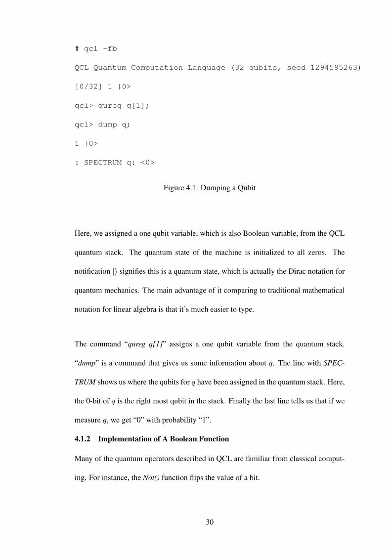
Figure 4.1: Dumping a Qubit
Here, we assigned a one qubit variable, which is also Boolean variable, from the QCL
quantum stack. The quantum state of the machine is initialized to all zeros. The
notification |〉 signifies this is a quantum state, which is actually the Dirac notation for
quantum mechanics. The main advantage of it comparing to traditional mathematical
notation for linear algebra is that it’s much easier to type.
The command “qureg q[1]” assigns a one qubit variable from the quantum stack.
“dump” is a command that gives us some information about q. The line with SPEC-
TRUM shows us where the qubits for q have been assigned in the quantum stack. Here,
the 0-bit of q is the right most qubit in the stack. Finally the last line tells us that if we
measure q, we get “0” with probability “1”.
4.1.2 Implementation of A Boolean Function
Many of the quantum operators described in QCL are familiar from classical comput-
ing. For instance, the Not() function flips the value of a bit.
30
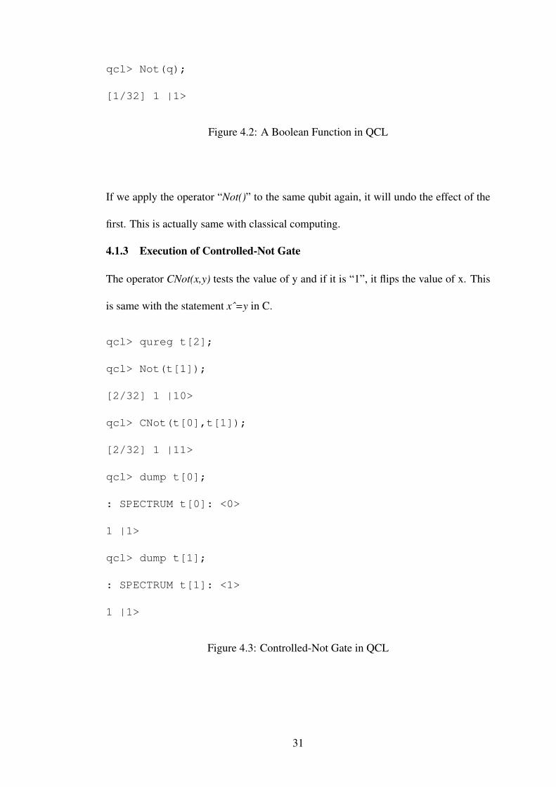
qcl> Not(q);
[1/32] 1 |1>
Figure 4.2: A Boolean Function in QCL
If we apply the operator “Not()” to the same qubit again, it will undo the effect of the
first. This is actually same with classical computing.
4.1.3 Execution of Controlled-Not Gate
The operator CNot(x,y) tests the value of y and if it is “1”, it flips the value of x. This
is same with the statement xˆ=y in C.
qcl> qureg t[2];
qcl> Not(t[1]);
[2/32] 1 |10>
qcl> CNot(t[0],t[1]);
[2/32] 1 |11>
qcl> dump t[0];
: SPECTRUM t[0]: <0>
1 |1>
qcl> dump t[1];
: SPECTRUM t[1]: <1>
1 |1>
Figure 4.3: Controlled-Not Gate in QCL
31
The operator CNot() is its own inverse just like the operator Not(). If we apply it again
to the same qubits, it will reverse the effect of the first, making the state same with the
starting state.
In fact, the idea of reversibility is very important to understand the quantum computing.
Theoretical physics reveals that every operation on quantum bits must be reversible,
except for measurement. That’s why, it is important to always keep enough information
to work any operation backwards. Hence, the classical operations like assignment
(x = y), AND (x& = y), and OR (x| = y) have to be modified to use in quantum
computing.
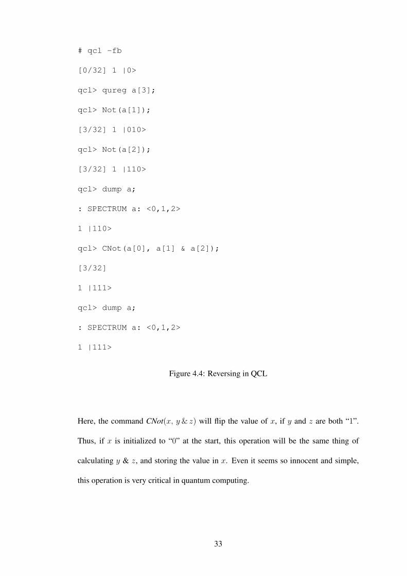
4.1.4 Way of Reversing a Boolean Operator
Luckily, there is a straight forward formula to convert irreversible classical operations
into quantum operations. First of all, never overwrite a quantum bit except to initialize
it to “0”. So, if we need to make an assignment (x = y), instead of this, we initialize
the target (x = 0), and use exclusive or (xˆ = y) as in the above example.
32
# qcl -fb
[0/32] 1 |0>
qcl> qureg a[3];
qcl> Not(a[1]);
[3/32] 1 |010>
qcl> Not(a[2]);
[3/32] 1 |110>
qcl> dump a;
: SPECTRUM a: <0,1,2>
1 |110>
qcl> CNot(a[0], a[1] & a[2]);
[3/32]
1 |111>
qcl> dump a;
: SPECTRUM a: <0,1,2>
1 |111>
Figure 4.4: Reversing in QCL
Here, the command CNot(x, y& z) will flip the value of x, if y and z are both “1”.
Thus, if x is initialized to “0” at the start, this operation will be the same thing of
calculating y & z, and storing the value in x. Even it seems so innocent and simple,
this operation is very critical in quantum computing.
33
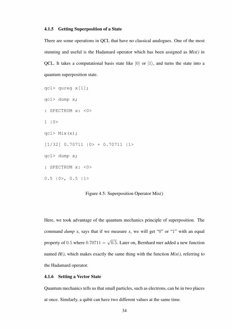
4.1.5 Getting Superposition of a State
There are some operations in QCL that have no classical analogues. One of the most
stunning and useful is the Hadamard operator which has been assigned as Mix() in
QCL. It takes a computational basis state like |0〉 or |1〉, and turns the state into a
quantum superposition state.
qcl> qureg x[1];
qcl> dump x;
: SPECTRUM x: <0>
1 |0>
qcl> Mix(x);
[1/32] 0.70711 |0> + 0.70711 |1>
qcl> dump x;
: SPECTRUM x: <0>
0.5 |0>, 0.5 |1>
Figure 4.5: Superposition Operator Mix()
Here, we took advantage of the quantum mechanics principle of superposition. The
command dump x, says that if we measure x, we will get “0” or “1” with an equal
property of 0.5 where 0.70711 =√
0.5. Later on, Bernhard mer added a new function
named H(), which makes exactly the same thing with the function Mix(), referring to
the Hadamard operator.
4.1.6 Setting a Vector State
Quantum mechanics tells us that small particles, such as electrons, can be in two places
at once. Similarly, a qubit can have two different values at the same time.
34
Despite a classical computer where the state of the machine is merely a single string of
ones and zeros, the state of a quantum computer is a vector with components for every
possible string of 1s and 0s. On the other hand, the strings of ones and zeros form the
basis for a vector space where our machine state lives. So, we can write down the state
of a quantum computer by writing out a sum like:
a|X>+ b|Y\> + ...
Figure 4.6: Quantum Computer with a Vector State
X and Y are strings of 1s and 0s, and a and b are the amplitudes for the respective
components X and Y. The notation |X〉 is just the way physicists denote a vector or a
state called X.
When the Hadamard operator Mix() applied to a bit in the state |0〉, it will transform
the state into sqrt (0.5) (|0〉+ |1〉) as we had in the above example (4.5). But, if we
apply Mix() to a bit which is in the state |1〉, we get sqrt (0.5) (|0〉 − |1〉). Thus, if we
apply Mix() twice to any qubit in any state, we get back to where we started. In other
words, the operator Mix() is it’s own inverse.
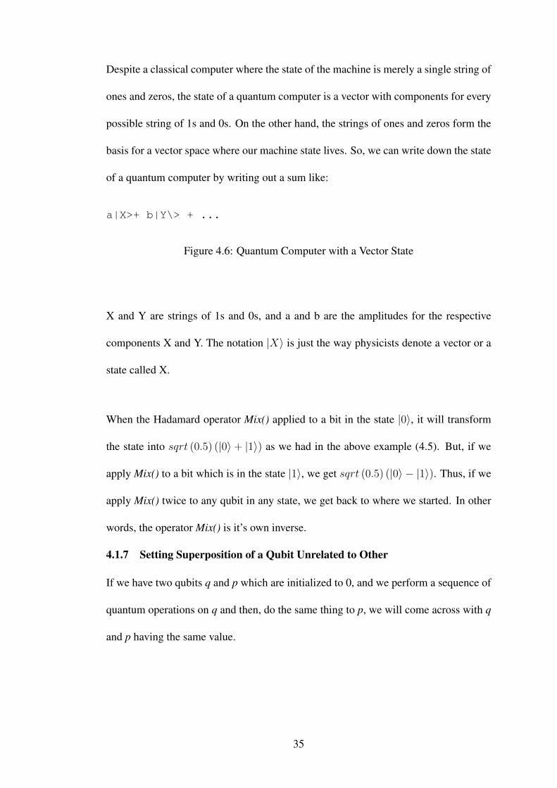
4.1.7 Setting Superposition of a Qubit Unrelated to Other
If we have two qubits q and p which are initialized to 0, and we perform a sequence of
quantum operations on q and then, do the same thing to p, we will come across with q
and p having the same value.
35
qcl> qureg q[1];
qcl> Not(q);
[1/32] 1 |1>
qcl> Mix(q);
[1/32] 0.70711 |0> - 0.70711 |1>
qcl> qureg p[1];
qcl> Not(p);
[2/32] 0.70711 |0,1> - 0.70711 |1,1>
qcl> Mix(p);
[2/32] 0.5 |0,0> - 0.5 |1,0> - 0.5 |0,1> + 0.5 |1,1>
qcl> dump q;
: SPECTRUM q: <0>
0.5 |0>, 0.5 |1>
qcl> dump p;
: SPECTRUM p: <1>
0.5 |0>, 0.5 |1>
Figure 4.7: Unrelated Qubits in Superposition States
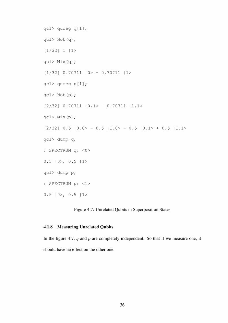
4.1.8 Measuring Unrelated Qubits
In the figure 4.7, q and p are completely independent. So that if we measure one, it
should have no effect on the other one.
36
qcl> measure q;
[2/8] -0.70711 |0> + 0.70711 |1>
qcl> dump p
: SPECTRUM b: |0>
0.5 |0>, 0.5 |1>
Figure 4.8: Measuring Unrelated Qubits
As we see, the spectrum of p was unchanged by measuring q. On the other hand, if the
operations were more complicated than simple operators like Not() or Mix(), we might
be allured to perform them only once on a and then, copy the value from q to p. In fact,
we cannot copy it because it’s not a reversible operation, however we can initialize p
to 0 and CNot(p,q) which performs the same goal.
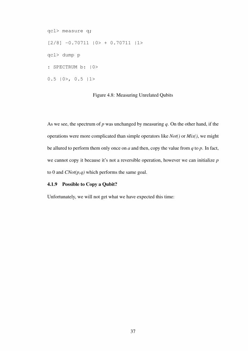
4.1.9 Possible to Copy a Qubit?
Unfortunately, we will not get what we have expected this time:
37
qcl> qureg q[1];
qcl> Not(q);
[1/32] 1 |1>
qcl> Mix(q);
[1/32] 0.70711 |0> - 0.70711 |1>
qcl> qureg p[1];
qcl> CNot(p,q);
[2/32] 0.70711 |0,0> - 0.70711 |1,1>
qcl> dump q;
: SPECTRUM q: <0>
0.5 |0>, 0.5 |1>
qcl> dump p;
: SPECTRUM p: <1>
0.5 |0>, 0.5 |1>
Figure 4.9: Preparing State for Copy
The spectrum of p and q seem alright, and of courseif we measure p or q alone, we will
get the same result as above. But the difference lies in what happens when we measure
both p and q.
4.1.10 Superposition of Qubits is Crushed
Note that the outcome of a measurement is random. Thus, if we repeat this operation,
the result may change.
38
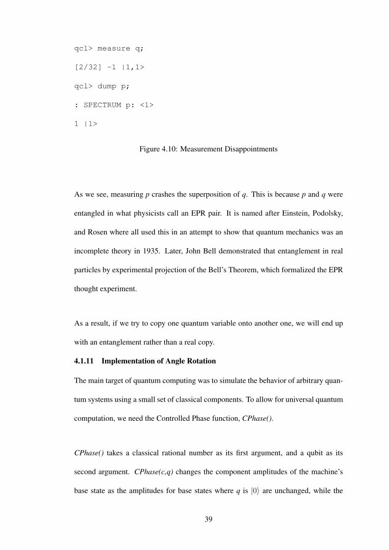
qcl> measure q;
[2/32] -1 |1,1>
qcl> dump p;
: SPECTRUM p: <1>
1 |1>
Figure 4.10: Measurement Disappointments
As we see, measuring p crashes the superposition of q. This is because p and q were
entangled in what physicists call an EPR pair. It is named after Einstein, Podolsky,
and Rosen where all used this in an attempt to show that quantum mechanics was an
incomplete theory in 1935. Later, John Bell demonstrated that entanglement in real
particles by experimental projection of the Bell’s Theorem, which formalized the EPR
thought experiment.
As a result, if we try to copy one quantum variable onto another one, we will end up
with an entanglement rather than a real copy.
4.1.11 Implementation of Angle Rotation
The main target of quantum computing was to simulate the behavior of arbitrary quan-
tum systems using a small set of classical components. To allow for universal quantum
computation, we need the Controlled Phase function, CPhase().
CPhase() takes a classical rational number as its first argument, and a qubit as its
second argument. CPhase(c,q) changes the component amplitudes of the machine’s
base state as the amplitudes for base states where q is |0〉 are unchanged, while the
39
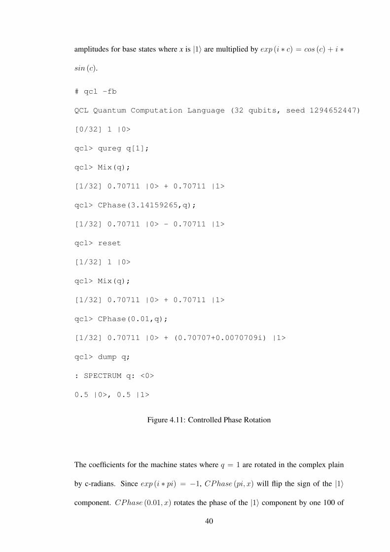
amplitudes for base states where x is |1〉 are multiplied by exp (i ∗ c) = cos (c) + i ∗
sin (c).
# qcl -fb
QCL Quantum Computation Language (32 qubits, seed 1294652447)
[0/32] 1 |0>
qcl> qureg q[1];
qcl> Mix(q);
[1/32] 0.70711 |0> + 0.70711 |1>
qcl> CPhase(3.14159265,q);
[1/32] 0.70711 |0> - 0.70711 |1>
qcl> reset
[1/32] 1 |0>
qcl> Mix(q);
[1/32] 0.70711 |0> + 0.70711 |1>
qcl> CPhase(0.01,q);
[1/32] 0.70711 |0> + (0.70707+0.0070709i) |1>
qcl> dump q;
: SPECTRUM q: <0>
0.5 |0>, 0.5 |1>
Figure 4.11: Controlled Phase Rotation
The coefficients for the machine states where q = 1 are rotated in the complex plain
by c-radians. Since exp (i ∗ pi) = −1, CPhase (pi, x) will flip the sign of the |1〉
component. CPhase (0.01, x) rotates the phase of the |1〉 component by one 100 of
40
a radian in the complex plane. The parenthesized tuple (0.70707, 0.0070709i) is the
QCL representation of the complex number exp (0.01 ∗ i) = 0.70707+ i∗0.0070709i.
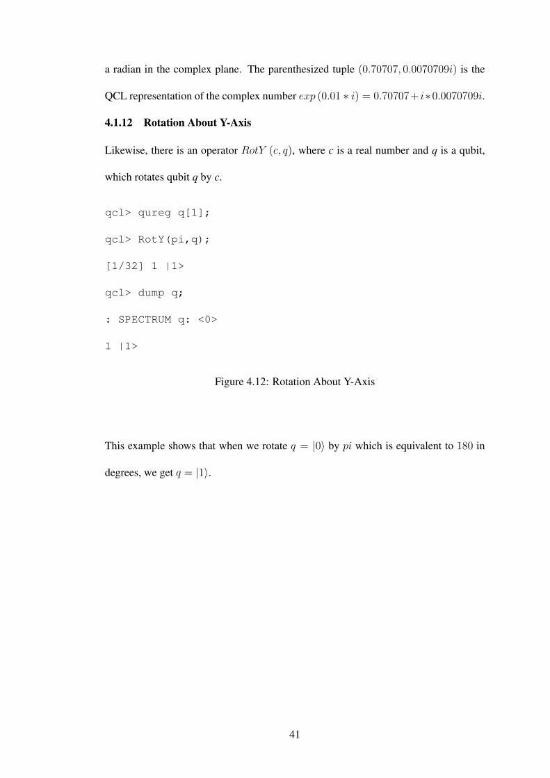
4.1.12 Rotation About Y-Axis
Likewise, there is an operator RotY (c, q), where c is a real number and q is a qubit,
which rotates qubit q by c.
qcl> qureg q[1];
qcl> RotY(pi,q);
[1/32] 1 |1>
qcl> dump q;
: SPECTRUM q: <0>
1 |1>
Figure 4.12: Rotation About Y-Axis
This example shows that when we rotate q = |0〉 by pi which is equivalent to 180 in
degrees, we get q = |1〉.
41
qcl> qureg q[1];
qcl> RotY(pi/2,q);
[1/32] 0.70711 |0> + 0.70711 |1>
qcl> dump q;
: SPECTRUM q: <0>
0.5 |0>, 0.5 |1>
qcl> reset
[1/32] 1 |0>
qcl> Mix(q);
[1/32] 0.70711 |0> + 0.70711 |1>
qcl> dump q;
: SPECTRUM q: <0>
0.5 |0>, 0.5 |1>
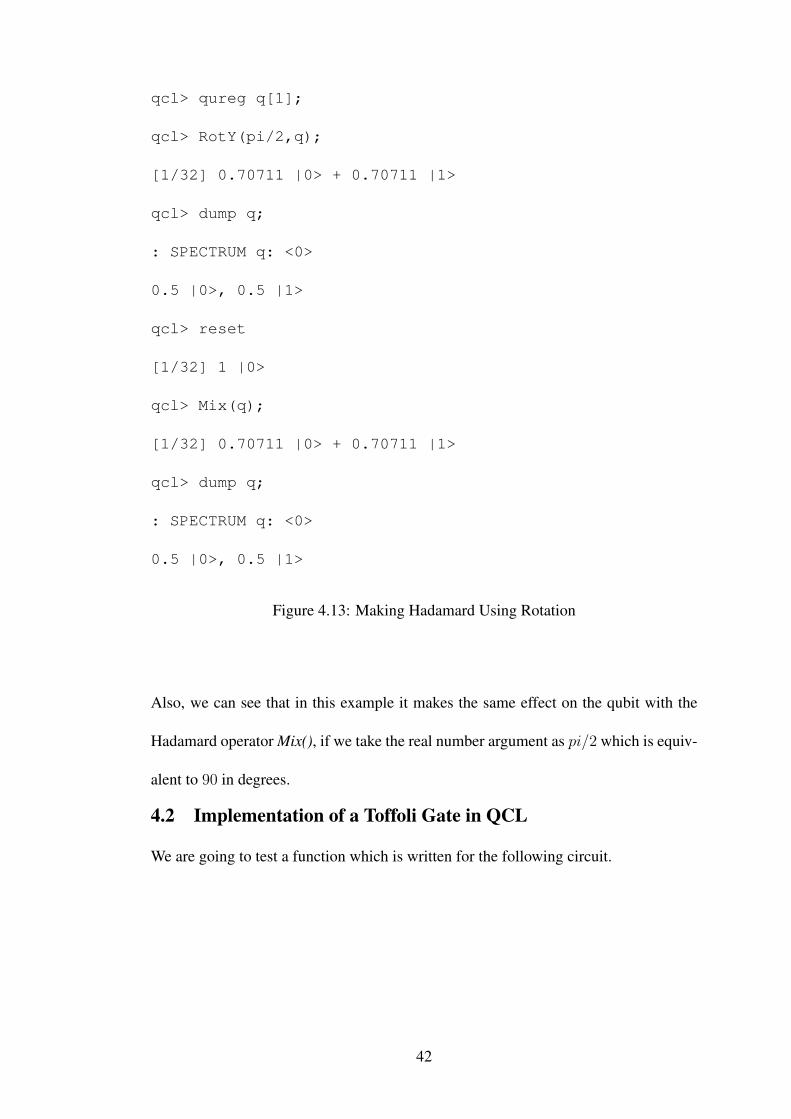
Figure 4.13: Making Hadamard Using Rotation
Also, we can see that in this example it makes the same effect on the qubit with the
Hadamard operator Mix(), if we take the real number argument as pi/2 which is equiv-
alent to 90 in degrees.
4.2 Implementation of a Toffoli Gate in QCL
We are going to test a function which is written for the following circuit.
42
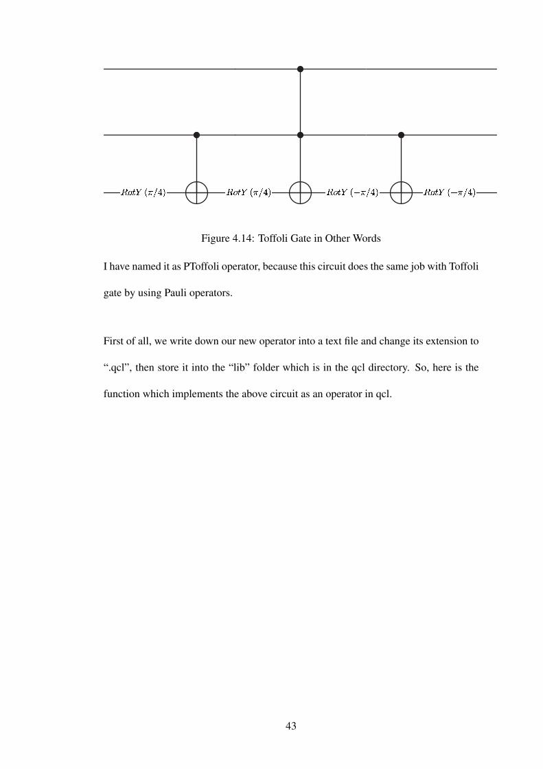
Figure 4.14: Toffoli Gate in Other Words
I have named it as PToffoli operator, because this circuit does the same job with Toffoli
gate by using Pauli operators.
First of all, we write down our new operator into a text file and change its extension to
“.qcl”, then store it into the “lib” folder which is in the qcl directory. So, here is the
function which implements the above circuit as an operator in qcl.
43
operator ptoffoli(qureg q)
{
const n=#q;
int i;
int m;
m=2*n-3;
RotY(-pi/4,q[n-1]);
for i=1 to m
{ if n-(1+i)<=0
{ CNot(q[n-1],q[(1+i)-n]);
RotY(pi/4,q[n-1]); }
else
{ CNot(q[n-1],q[n-(1+i)]);
RotY(-pi/4,q[n-1]); }
}
}
Figure 4.15: PToffoli Operator
Now, let’s consider if this function works or not on examples with an input q with
three qubits by using qcl. To demonstrate that this operator works, we will do the same
steps, that the operator does, manually on qcl.
44
4.2.1 Example with the Input q[3] = |000〉
qcl> qureg q[3];
qcl> RotY(-pi/4,q[2]);
[3/32] 0.92388 |000> - 0.38268 |100>
qcl> CNot(q[2],q[1]);
[3/32] 0.92388 |000> - 0.38268 |100>
qcl> RotY(-pi/4,q[2]);
[3/32] 0.70711 |000> - 0.70711 |100>
qcl> CNot(q[2],q[0]);
[3/32] 0.70711 |000> - 0.70711 |100>
qcl> RotY(pi/4,q[2]);
[3/32] 0.92388 |000> - 0.38268 |100>
qcl> CNot(q[2],q[1]);
[3/32] 0.92388 |000> - 0.38268 |100>
qcl> RotY(pi/4,q[2]);
[3/32] 1 |000>
Figure 4.16: Input q[3] = |000〉
As we see, the CNot operators don’t do anything because the control qubits are 0. So,
at the end, the qubit becomes same as previous, just as our function says:
45
qcl> include "ptoffoli.qcl";
qcl> qureg q[3];
qcl> ptoffoli(q);
[3/32] 1 |000>
Figure 4.17: PToffoli with q[3] = |000〉
4.2.2 Example with the Input q[3] = |010〉
qcl> Not(q[1]);
[3/32] 1 |010>
qcl> RotY(-pi/4,q[2]);
[3/32] 0.92388 |010> - 0.38268 |110>
qcl> CNot(q[2],q[1]);
[3/32] -0.38268 |010> + 0.92388 |110>
qcl> RotY(-pi/4,q[2]);
[3/32] 1 |110>
qcl> CNot(q[2],q[0]);
[3/32] 1 |110>
qcl> RotY(pi/4,q[2]);
[3/32] -0.38268 |010> + 0.92388 |110>
qcl> CNot(q[2],q[1]);
[3/32] 0.92388 |010> - 0.38268 |110>
qcl> RotY(pi/4,q[2]);
[3/32] 1 |010>
Figure 4.18: Input q[3] = |010〉
46
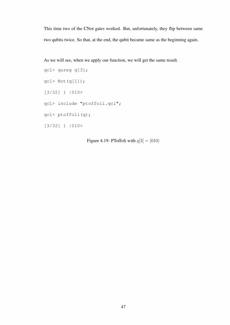
This time two of the CNot gates worked. But, unfortunately, they flip between same
two qubits twice. So that, at the end, the qubit became same as the beginning again.
As we will see, when we apply our function, we will get the same result.
qcl> qureg q[3];
qcl> Not(q[1]);
[3/32] 1 |010>
qcl> include "ptoffoli.qcl";
qcl> ptoffoli(q);
[3/32] 1 |010>
Figure 4.19: PToffoli with q[3] = |010〉
47
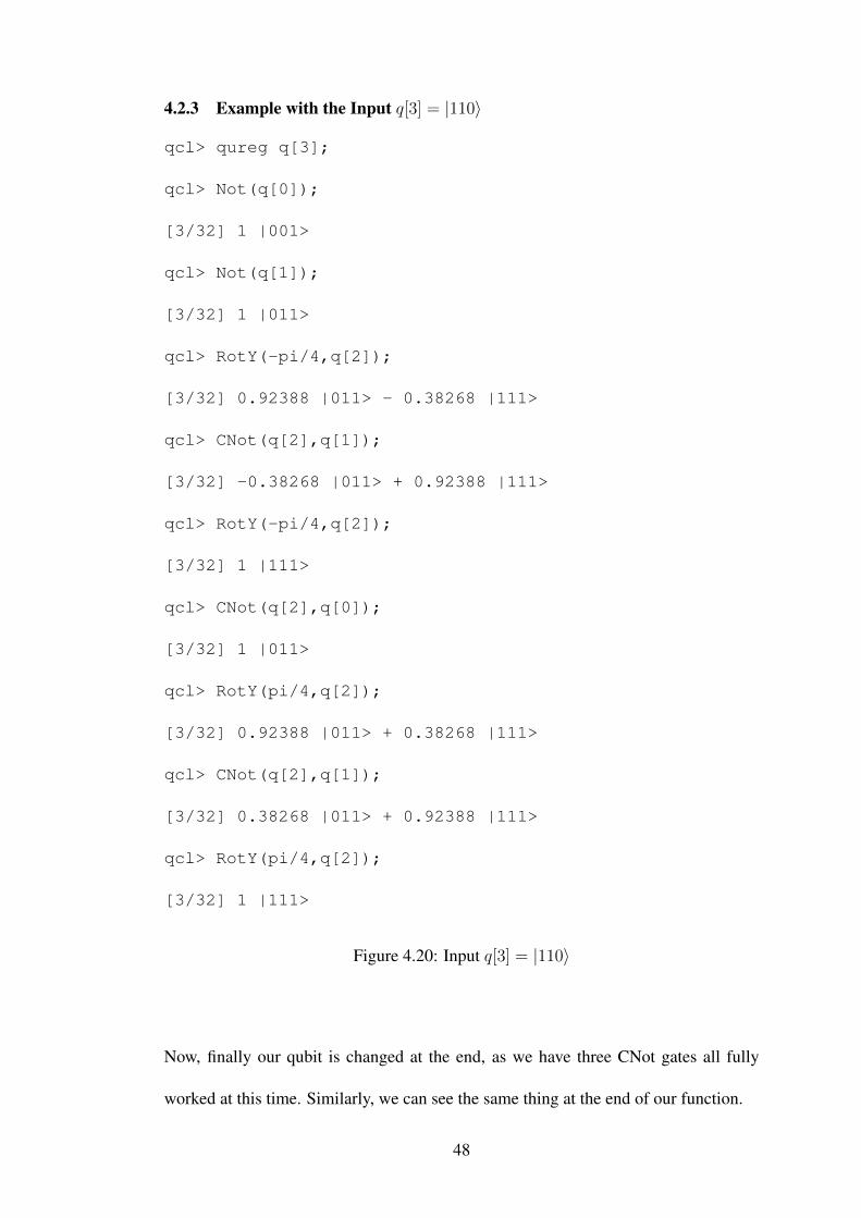
4.2.3 Example with the Input q[3] = |110〉
qcl> qureg q[3];
qcl> Not(q[0]);
[3/32] 1 |001>
qcl> Not(q[1]);
[3/32] 1 |011>
qcl> RotY(-pi/4,q[2]);
[3/32] 0.92388 |011> - 0.38268 |111>
qcl> CNot(q[2],q[1]);
[3/32] -0.38268 |011> + 0.92388 |111>
qcl> RotY(-pi/4,q[2]);
[3/32] 1 |111>
qcl> CNot(q[2],q[0]);
[3/32] 1 |011>
qcl> RotY(pi/4,q[2]);
[3/32] 0.92388 |011> + 0.38268 |111>
qcl> CNot(q[2],q[1]);
[3/32] 0.38268 |011> + 0.92388 |111>
qcl> RotY(pi/4,q[2]);
[3/32] 1 |111>
Figure 4.20: Input q[3] = |110〉
Now, finally our qubit is changed at the end, as we have three CNot gates all fully
worked at this time. Similarly, we can see the same thing at the end of our function.
48
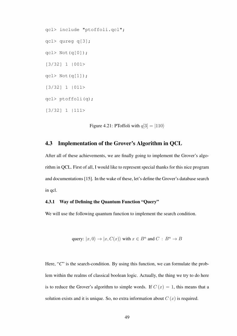
qcl> include "ptoffoli.qcl";
qcl> qureg q[3];
qcl> Not(q[0]);
[3/32] 1 |001>
qcl> Not(q[1]);
[3/32] 1 |011>
qcl> ptoffoli(q);
[3/32] 1 |111>
Figure 4.21: PToffoli with q[3] = |110〉
4.3 Implementation of the Grover’s Algorithm in QCL
After all of these achievements, we are finally going to implement the Grover’s algo-
rithm in QCL. First of all, I would like to represent special thanks for this nice program
and documentations [15]. In the wake of these, let’s define the Grover’s database search
in qcl.
4.3.1 Way of Defining the Quantum Function “Query”
We will use the following quantum function to implement the search condition.
query: |x, 0〉 → |x,C(x)〉 with x ∈ Bn and C : Bn → B
Here, “C” is the search-condition. By using this function, we can formulate the prob-
lem within the realms of classical boolean logic. Actually, the thing we try to do here
is to reduce the Grover’s algorithm to simple words. If C (x) = 1, this means that a
solution exists and it is unique. So, no extra information about C (x) is required.
49
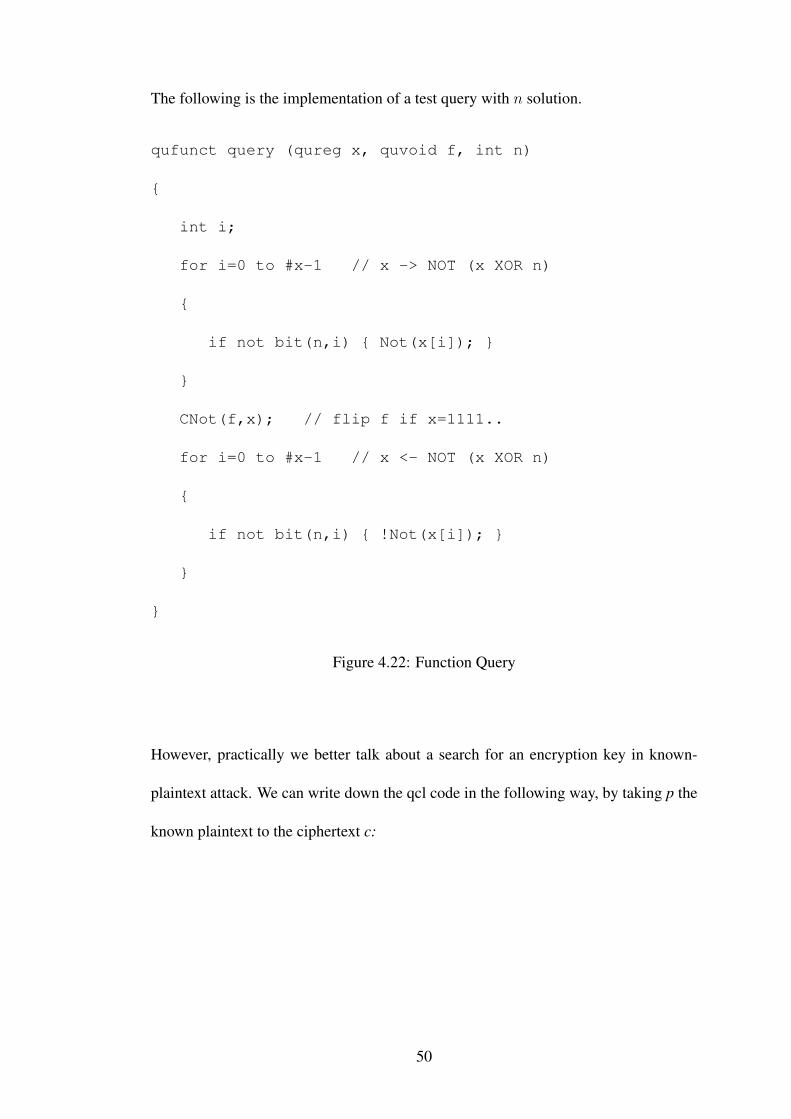
The following is the implementation of a test query with n solution.
qufunct query (qureg x, quvoid f, int n)
{
int i;
for i=0 to #x-1 // x -> NOT (x XOR n)
{
if not bit(n,i) { Not(x[i]); }
}
CNot(f,x); // flip f if x=1111..
for i=0 to #x-1 // x <- NOT (x XOR n)
{
if not bit(n,i) { !Not(x[i]); }
}
}
Figure 4.22: Function Query
However, practically we better talk about a search for an encryption key in known-
plaintext attack. We can write down the qcl code in the following way, by taking p the
known plaintext to the ciphertext c:
50

qufunct encrypt (int p, quconst key, quvoid c) { ... }
qufunct query (int c, int p, quconst key, quvoid f)
{
int i;
quscratch s[blocklength];
encrypt(p, key, s);
for i=0 to #s-1 // x <- NOT (x XOR n)
{
if not bit(p, i) { Not(x[i]); }
}
CNot(f, x); //flip f if s=1111...
}
Figure 4.23: Query for Text
Despite the previous example, this function utilizes a local scratch register which
makes it unnecessary to uncompute s.
4.3.2 How to Set up the Search Space
In a quantum computer, search space Bn, which is the solution space of a n bit query
condition C, can be executed as a superposition of all eigenstates of an n qubit register.
|ψ〉 =1√N
N∑i=0
|i〉 with N = 2n
Note that, we had talked about the implementation of the Hadamard operator in qcl in
4.1.5 which we use to prepare such a state.
51
4.3.3 The Principle Loop of the Algorithm
This consists of two steps.
1. Execute a conditional phase shift (4.1.11) to rotate the phase of all eigenvectors
which match the condition C by π radians.
Q : |i〉 →
− |i〉 if C (i)
|i〉 if not C (i)
2. Apply the diffusion operator
D =∑ij
|i〉 dij 〈j| with dij =
2N− 1 if i = j
2N
if not i = j
Since only one eigenvector |i0〉 is going to match the search condition C, the condi-
tional phase shift operator will turn the initial superposition into
|ψ′〉 = − 1√N|i0〉+
1√N
∑i 6=i0
|i〉 .
Then, the effect of the diffusion operator on an arbitrary eigenvector |i〉 is
D |i〉 = − |i〉+2
N
N−1∑j=0
|j〉
and an iteration on a state of the form
|ψ (k, l)〉 = k |i0〉+∑i 6=i0
l |i〉
refers to
|ψ (k, l)〉 Q−→ |ψ (−k, l)〉 D−→∣∣∣∣ψ(N − 2
Nk +
2 (N − 1)
Nl,N − 2
Nl − 2
Nk
)⟩
52
4.3.4 The Number of Iterations Needed
If we apply the above main loop repeatedly to the initial superposition
|ψ〉 =
∣∣∣∣ψ( 1√N,
1√N
)⟩=
1√N
N−1∑i=0
|i〉
the resulting state will be in the form |ψ (k, l)〉 and the complex amplitudes k and l are
described by the following system of recursions:
kj+1 =N − 2
Nkj +
2 (N − 1)
Nlj
lj+1 =N − 2
Nlj −
2
Nkj
By substituting sin2θ = 1N
, we can rewrite this system in the following closed form.
kj = sin ((2j + 1) θ)
lj =1√
N − 1cos ((2j + 1) θ)
The probability p of measuring i0 is given as p = k2, and it’s maximum state is θ =
π2(2j+1)
. Thus, for large lists 1√N� 1 we can assume sinθ ≈ θ and π � 2θ where the
number of iterations m for at most p is about m =⌊π4
√N⌋
with p > N−1N
. Also, if we
have p > 12, then m =
⌈π8
√N⌉
iterations will be enough.
4.3.5 The Implementation of the Query Operator
The operator Q can be constructed as in the following way, if we formulate the query
as we have mentioned in 4.3.1 before with a flag qubit f to allow for a strictly classical
implementation.
Q = query† (x, f)V (π) (f) query (x, f)
where V (φ) is the conditional phase gate.
53
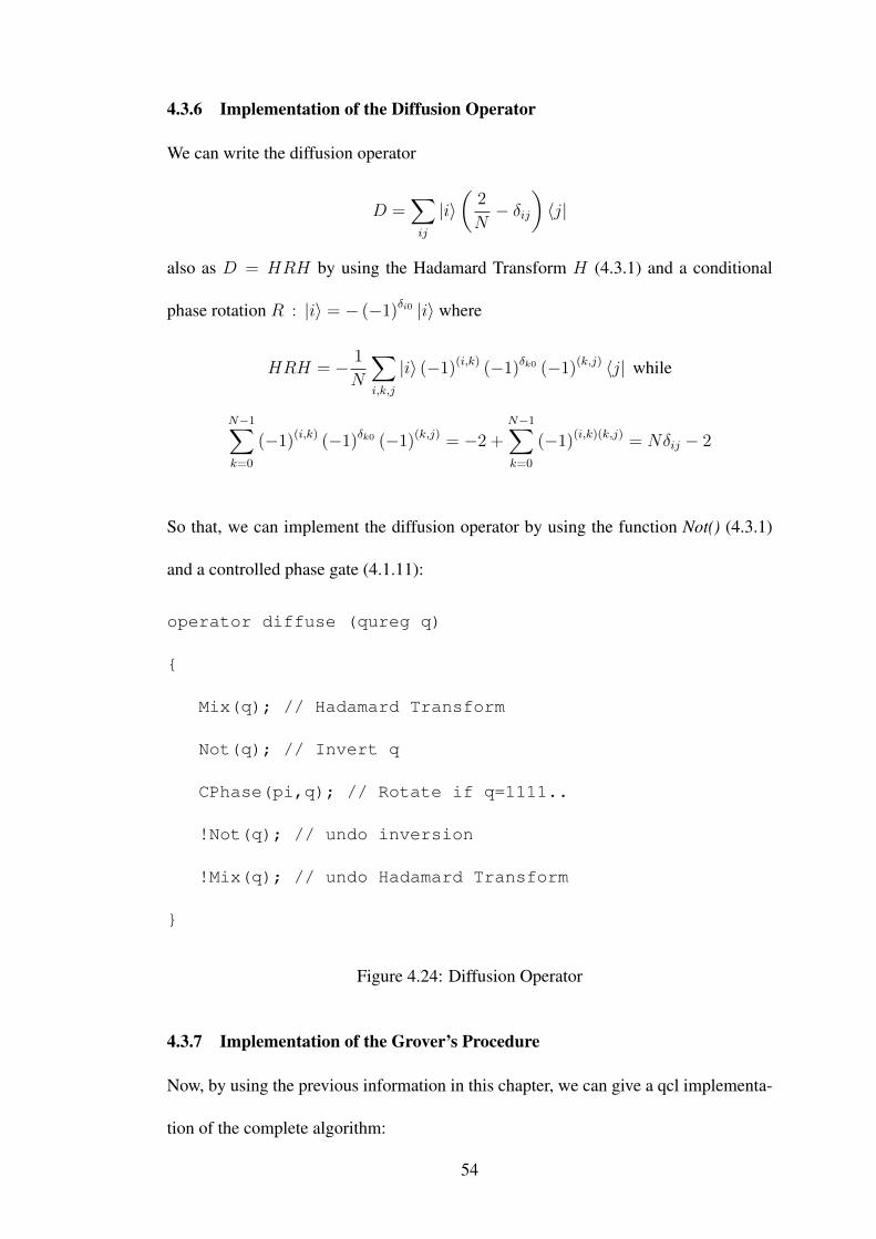
4.3.6 Implementation of the Diffusion Operator
We can write the diffusion operator
D =∑ij
|i〉(
2
N− δij
)〈j|
also as D = HRH by using the Hadamard Transform H (4.3.1) and a conditional
phase rotation R : |i〉 = − (−1)δi0 |i〉 where
HRH = − 1
N
∑i,k,j
|i〉 (−1)(i,k) (−1)δk0 (−1)(k,j) 〈j| while
N−1∑k=0
(−1)(i,k) (−1)δk0 (−1)(k,j) = −2 +N−1∑k=0
(−1)(i,k)(k,j) = Nδij − 2
So that, we can implement the diffusion operator by using the function Not() (4.3.1)
and a controlled phase gate (4.1.11):
operator diffuse (qureg q)
{
Mix(q); // Hadamard Transform
Not(q); // Invert q
CPhase(pi,q); // Rotate if q=1111..
!Not(q); // undo inversion
!Mix(q); // undo Hadamard Transform
}
Figure 4.24: Diffusion Operator
4.3.7 Implementation of the Grover’s Procedure
Now, by using the previous information in this chapter, we can give a qcl implementa-
tion of the complete algorithm:
54
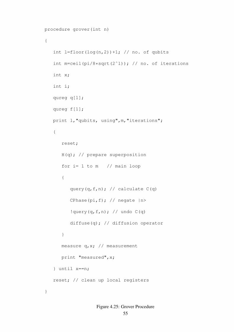
procedure grover(int n)
{
int l=floor(log(n,2))+1; // no. of qubits
int m=ceil(pi/8*sqrt(2ˆl)); // no. of iterations
int x;
int i;
qureg q[l];
qureg f[1];
print l,"qubits, using",m,"iterations";
{
reset;
H(q); // prepare superposition
for i= 1 to m // main loop
{
query(q,f,n); // calculate C(q)
CPhase(pi,f); // negate |n>
!query(q,f,n); // undo C(q)
diffuse(q); // diffusion operator
}
measure q,x; // measurement
print "measured",x;
} until x==n;
reset; // clean up local registers
}
Figure 4.25: Grover Procedure55
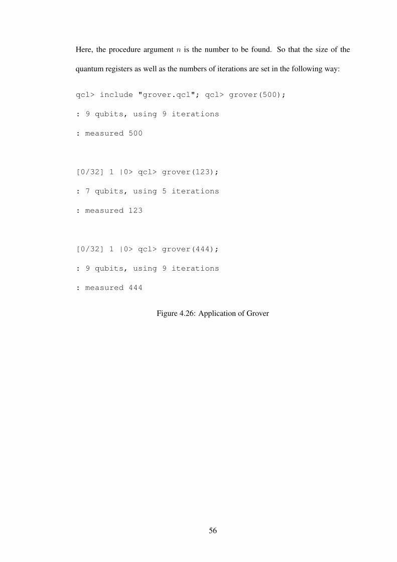
Here, the procedure argument n is the number to be found. So that the size of the
quantum registers as well as the numbers of iterations are set in the following way:
qcl> include "grover.qcl"; qcl> grover(500);
: 9 qubits, using 9 iterations
: measured 500
[0/32] 1 |0> qcl> grover(123);
: 7 qubits, using 5 iterations
: measured 123
[0/32] 1 |0> qcl> grover(444);
: 9 qubits, using 9 iterations
: measured 444
Figure 4.26: Application of Grover
56
CONCLUSION
Among this thesis, we have talked about one of the best algorithms of the quantum
computing, which was Grover’s algorithm. Also, we have taken a look with the eye of
complexity to this algorithm, and finalized with the implementation of it in an abstract
quantum computer with the help of a quantum programming language, which was
QCL. Even now, while you read this thesis, computer engineers and programmers are
probably finding new achievements about quantum computer and its programming.
But, this still doesn’t change the fact that it will take many years to construct a quantum
computer. These achievements certainly includes also some papers or theses, where
many might have no effect in the improvement of quantum computers. Even though,
the main idea should be here to go ahead with trustworthy steps, and to be a part of
one of the most amazing invention of next generation.
57
Appendix
58
Appendix A: Investigating Complexity
A.1 Nondeterministic
Recall that in computer science nondeterministic algorithm is an algorithm that defines
multiple ways of processing the same input, without any specification of which one
will be taken.
A.2 Polynomial Time
An algorithm is said to be polynomial time if its running time is upper bounded by a
polynomial in the size of the input for the algorithm.
A.3 Turing Machine
It is a theoretical device that manipulates symbols on a strip of tape according to a table
of rules. Despite its simplicity, a Turing machine can be adapted to simulate the logic
of any computer algorithm, and is particularly useful in explaining the functions of a
CPU inside a computer[11].
A.4 Decision Problems
In computational complexity theory, a decision problem is a question in some formal
system with a yes-or-no answer, depending on the values of some input parameters.
A.5 Polynomial Time Reduction
A polynomial-time reduction or a polynomial-time Turing reduction is a reduction
which is computable by a deterministic Turing machine in polynomial time.
A.6 Boolean Logic
It is the part of logic with the elements (or “bits”) each contain only two possible
values, called various names, such as “true” and “false”, “yes” and “no”, “on” and
59
“off”, or “1” and “0”.
A.7 SAT Problem
In full name, it is the Boolean satisfiability problem. Satisfiability is the problem of
determining if the variables of a given Boolean formula can be assigned in such a way
as to make the formula evaluate to TRUE. Another important thing is to determine
whether no such assignments exist, which would imply that the function expressed by
the formula is identically FALSE for all possible variable assignments. In this case,
we call the function is unsatisfiable; otherwise it is satisfiable.
A.8 Complexity Class
It is a set of problems of related resource-based complexity. For instances, the class
NP is the set of decision problems that can be solved by a non-deterministic Turing
machine in polynomial time, and the class PSPACE is the set of decision problems that
can be solved by a deterministic Turing machine in polynomial space.
A.9 Class NP
In computational complexity theory, NP refers to nondeterministic polynomial time. It
is the set of all decision problems for which the instances where the answer is “yes”
have efficiently verifiable proofs of the fact that the answer is indeed “yes”. Particu-
larly, these proofs have to be verifiable in polynomial time by a deterministic Turing
machine. In more formal words, NP is the set of decision problems where the “yes” in-
stances can be recognized in polynomial time by a non-deterministic Turing machine.
A.10 Class NP-complete
It is a class of decision problems. A problem L is called NP-complete if it has following
two properties:
60
1. It is in the set of NP problems: Any given solution to L can be verified quickly
that is in polynomial time.
2. It is also in the set of NP-hard problems: Any NP problem can be converted into
L by a transformation of the inputs in polynomial time.
A.11 Class NP-Hard
It is a class of problems that are “at least as hard as the hardest problems in NP”. A
problem K is NP-hard if and only if there is an NP-complete problem L that is polyno-
mial time Turing reducible to H. In other words, L can be solved in polynomial time
by an oracle machine with an oracle for H. Informally, we can think of an algorithm
that can call such an oracle machine as a subroutine for solving H, and solves L in
polynomial time, if the subroutine call takes only one step to compute.
61
REFERENCES
[1] S. Aaronson. Lower bounds for local search by quantum arguments. 2004.
[2] S. Arora and B. Barak. Computational Complexity A Modern Approach. Cam-
bridge University Press, 2009.
[3] G. Chen and R. K. Brylinski. Mathematics of Quantum Computation. Chapman
and Hall/CRC, 2002.
[4] K. L. Grover. Quantum mechanics helps in searching for a needle in a haystack.
1997.
[5] B. Huntting, and D. Mertz. An Introduction To Quantum Computing: A Guide
to Solving Intractable Problems Simply 2001 http://gnosis.cx/.
[6] P. Kaye, R. Laflamme, and M. Mosca. An Introduction to Quantum Computing.
Oxford University Press, 2007.
[7] N. D. Mermin. Quantum Computer Science An Introduction. Cambridge Univer-
sity Press, 2007.
[8] Micheal A. Nielsen and Isaac L. Chuang. Quantum Computation and Quantum
Information. Cambridge University Press, 2000.
[9] K. L. Grover. A Fast Quantum Mechanical Algorithm for Database Search. 1996.
62
[10] E. Rieffel and W. Polak. An introduction to quantum computing for non-
physicists. 2000.
[11] P. W. Shor. Introduction to Quantum Algorithms 2001.
[12] P. W. Shor. Polynomial-time algorithms for prime factorization and discrete loga-
rithms on a quantum computer. http://arXiv.org/abs/quant-ph/9508027v2, 1996.
[13] Grover K. L. Tulsi, T. and A. Patel. A new algorithm for fixed point quantum
search. 2006.
[14] B. Omer. A procedural formalism for quantum computing. Master’s thesis, Tech-
nical University of Vienna, 1998.
[15] B. Omer. Quantum programming in qcl. Master’s thesis, Technical University of
Vienna, 2000.
[16] B. Omer. Classical concepts in quantum programming. International Journal of
Theoretical Physics 44/7, pp. 943-955, 2005., 2002.
[17] B. Omer. Structured Quantum Programming. PhD thesis, Vienna University of
Technology, 2009.
63