6

EUROPEAN ECONOMY

Economic and Financial Affairs

ISSN 2443-8022 (online)

EUROPEAN ECONOMY

Growth Effects of Corporate Balance Sheet Adjustments in the EU:An Econometric & Model-based AssessmentRomanos Priftis, Anastasia Theofilakou

DISCUSSION PAPER 076 | MARCH 2018

European Economy Discussion Papers are written by the staff of the European Commission’s Directorate-General for Economic and Financial Affairs, or by experts working in association with them, to inform discussion on economic policy and to stimulate debate. The views expressed in this document are solely those of the author(s) and do not necessarily represent the official views of the European Commission. Authorised for publication by Mary Veronica Tovšak Pleterski, Director for Investment, Growth and Structural Reforms, and José Eduardo Leandro, Director for Policy, Strategy, Coordination and Communication.

LEGAL NOTICE

Neither the European Commission nor any person acting on behalf of the European Commission is responsible for the use that might be made of the information contained in this publication. This paper exists in English only and can be downloaded from https://ec.europa.eu/info/publications/economic-and-financial-affairs-publications_en.

Luxembourg: Publications Office of the European Union, 2018

PDF ISBN 978-92-79-77406-5 ISSN 2443-8022 doi:10.2765/018954 KC-BD-18-003-EN-N

© European Union, 2018 Non-commercial reproduction is authorised provided the source is acknowledged. For any use or reproduction of material that is not under the EU copyright, permission must be sought directly from the copyright holders.

European Commission Directorate-General for Economic and Financial Affairs

Growth Effects of CorporateBalance Sheet Adjustments in the EU: An Econometric and Model-based Assessment

Romanos Priftis and Anastasia Theofilakou

Abstract

This paper investigates the impact of active balance sheet adjustments in the non-financial corporate sector on economic growth in the EU. We first jointly model firms' ability to reduce their balance sheet imbalances and a growth equation in an instrumental variables (IV) panel context. This enables us to explicitly consider the contemporaneous interaction between corporate balance sheet adjustment and growth, which can otherwise bias inference. Our main findings inter alia suggest that: i) periods of active corporate deleveraging are associated on average with lower output growth compared to periods when no adjustment takes place, and ii) a decline in corporate debt overhang supports output growth. To explore the deleveraging mechanism qualitatively we then employ a banking variant of the Commission's QUEST model and show that following a deleveraging shock, triggered by a tightening of firms' collateral constraints, the effects on investment and GDP are negative in the short-run. In the medium run once corporate debt has been reduced the effects fade away allowing the economy to recover. In the long run the effects are largely neutral suggesting that the source of investment financing, be it financial intermediaries or the stock market, does not seem to matter.

JEL Classification: C3, E21, G2.

Keywords: corporate deleveraging, growth effects, IV estimation, DSGE model, collateral constraints, European Union.

Acknowledgements: We thank our referees Lucian Briciu and Daniel Monteiro for providing us with very helpful comments and suggestions. We are also thankful to Björn Döhring, Evelyne Hespel, Werner Roeger and Lukas Vogel for valuable suggestions and discussions. The views expressed in the paper are those of the authors and should not be attributed to the institutions to which they are affiliated.

Contact: Romanos Priftis, Bank of Canada, 234 Wellington Street, Ottawa, K1A 0G9, Ontario, Canada, rpriftis@bank-banque-canada.ca. Anastasia Theofilakou, DG for Economic Policy, Hellenic Ministry of Finance, Greece, a.theofilakou@mnec.gr. This work was completed during Priftis’ time at Directorate-General for Economic and Financial Affairs of the European Commission.

EUROPEAN ECONOMY Discussion Paper 076

CONTENTS EXECUTIVE SUMMARY 4

1. Introduction 5

2. Econometric specification 7

2.1. Identifying corporate balance sheet adjustments 7

2.2. Empirical model 8

2.3. Econometric results 11

2.4. Robustness checks 15

3. Corporate deleveraging and macroeconomic adjustment 16

3.1. Model overview 16

3.2. Simulations 18

4. Conclusions 21

REFERENCES 22

ECONOMETRIC RESULTS 25

APPENDIX

Data and sources 29

Statistical tests on IV estimates 29

LIST OF TABLES

A. Responses of macroeconomic aggregates 20

1. Corporate balance sheet adjustment episodes in the EU 25

2. Determinants and growth effects of corporate balance sheet adjustments in the EU 26

3. Robustness checks 27

4. Robustness checks: Instrument validity (CAPB) 28

LIST OF GRAPHS 1. Model ov erview 18

3

EXECUTIVE SUMMARY

This paper investigates the impact of active balance sheet adjustments in the non-financial corporate sector on economic growth in the EU. The approach used is both econometric as well as model-based.

• We first jointly estimate firms' ability to reduce their balance sheet imbalances and a growth equation in an instrumental variables (IV) panel context.

• We also assess econometrically the impact of corporate debt overhang on active corporate deleveraging and on economic growth in the EU.

• Our main econometric findings suggest that: i) periods of active corporate deleveraging are associated on average with lower output growth compared to periods when no adjustment takes place, and ii) a decline in corporate debt overhang supports output growth.

• In order to understand the dynamic aspects of corporate deleveraging, we employ a banking variant of the Commission's QUEST model.

• Corporate deleveraging is triggered through a tightening of the entrepreneurs' collateral constraint, leading to a reduction in loans.

• The effects on investment and GDP are negative in the short-run, but fade away and allow the economy to recover in the medium run, once entrepreneurs move away from banks to internal financing of their investment. In the long run, the effects are largely neutral.

• Although in principle financial intermediaries can attach an endogenous risk-premium to the loan rate that reflects corporate firms' safety and borrowing capacity, an analysis of the reduction in debt-overhang is not investigated in this context.

4

1. INTRODUCTION

A legacy of the recent financial crisis is the excessive stock of private sector debt, including high levels of corporate debt in some European economies. Active deleveraging in the non-financial corporate sector is associated with an increase in net savings either through lower investment, higher savings or both. This is commonly expected to have a more detrimental impact on growth compared to passive deleveraging, in which positive growth and valuation effects drive an improvement in debt ratios. In the academic literature, only a handful of studies have examined the impact of corporate debt on output growth. Cecchetti et al. (2011) investigate the presence of threshold effects of corporate debt on growth and find that corporate debt that exceeds 90% of GDP becomes a drag on growth. Bornhorst and Ruiz-Arranz (2013) find that high corporate debt and household debt are associated with negative growth, while the negative effects are stronger as the number of indebted sector in the economy increases. In particular, a 10 percentage point increase in the corporate debt-to-GDP ratio beyond the 98% average level is associated with a decline in average annual growth in the range of 7 to 11 basis points. Based on aggregated firm-level data, Goretti and Souto (2003) find a negative relationship between firms’ investment to-capital ratio and their debt burden in euro area periphery countries.

citly account for the potential feedback loops between active deleveraging and macroeconomic shocks.

aging (through the investment and/or the savings channel), but also on economic growth in the EU.

Based on national accounts data, Ruscher and Wolff (2012) investigate the determinants of corporate balance sheet adjustments in advanced economies and find that adverse macroeconomic conditions and balance sheet strength are important drivers of corporate balance sheet repair. However, changes in economic growth enter with a lag as a determinant in the balance sheet equation, capturing the effects of past macroeconomic conditions on corporate deleveraging. In a recent study, Bricongne and Mordonu (2015) define corporate deleveraging in terms of growth rates in the stock of debt and report important linkages between corporate and household debt reduction, mainly through the wage channel. By analysing a cross-country sample of both advanced and emerging economies, Chen et al. (2015) focus on the macroeconomic impact of total private sector debt. The authors define private sector deleveraging as the change in private sector debt-to-GDP ratio and examine the impact on growth from the size, duration and intensity of the deleveraging episodes. In a single equation setting, they find that a reduction by 10 percentage points in the private sector debt-to-GDP ratio is associated with an increase in annual growth of about 0.4 percentage points. Still, these latter studies do not expli

Based on an econometric approach, this paper investigates the effects of corporate balance sheet adjustments on economic growth in the EU. More specifically, first, we jointly model the ability of the non-financial corporate sector to correct its balance sheet and a growth equation in an instrumental variables (IV) panel context. Both economic growth and corporate balance sheet adjustments enter in the estimated system of simultaneous equations as endogenous variables. The novelty of this approach is that it enables us to explicitly consider the contemporaneous interaction between corporate balance sheet adjustment and economic growth, which can otherwise bias inference. Also, as opposed to passive deleveraging, the focus here lies on active deleveraging, namely on the deliberate increase of savings and/or decrease of investment by non-financial corporations, defined based on sectoral national accounts data. Compared to the relevant literature, the episodes of corporate balance sheet adjustment are extended over the recent years of the "double dip" recession, and subdued economic growth and investment dynamics in the EU. Finally, we also assess the impact of corporate debt overhang on active corporate delever

5

While the IV estimation lets the “data speak”, arguably, it only captures an average effect over the sample and does not shed light on the underlying dynamics of the main macroeconomic aggregates over time. In order to understand the dynamic aspects obtained from the econometric analysis, we subsequently employ a banking variant of the Commission's QUEST model to qualitatively offer a theoretical explanation for the empirical evidence obtained. The QUEST variant used is a closed economy model calibrated to the EU aggregate economy, which incorporates a banking sector with bank capital. We opt for this model variant as it distinguishes the household sector into savers and borrowers (entrepreneurs). Entrepreneurs maximise an intertemporal utility function over entrepreneurial consumption, subject to a budget constraint, a capital accumulation constraint and a collateral constraint. Corporate deleveraging is triggered through a tightening of the entrepreneurs' collateral constraint, leading to a reduction in loans and adversely affecting consumption, investment and growth in the short-run. Our main findings are summarised as follows. The empirical analysis confirms that there are two-way causality effects between economic growth and corporate balance sheet adjustments. Active corporate deleveraging, defined as large and persistent improvement in the net lending/borrowing position of the corporate sector, is driven by declines in economic growth. Lower growth signalling subdued demand seems to weigh on corporate balance sheets and results in depressed corporate investment and/or increased savings. However, expectations of low growth trigger corporate balance sheet corrections not only because firms do not need additional capacity but also because they are unwilling to maintain too high leverage. Lower growth can worsen expectations about future profitability, making further increases in the stock of debt more risky and their financing more difficult to obtain, thereby intensifying pressures for balance sheet repair. Indeed, we find that higher debt overhang, that reflects firms` incapacity to service their debt given their operating cash flows, can cause firms to underinvest, and/or increase savings usually through cuts in the wage bill. In support of relevant theoretical views, we also find that long term debt is the main channel of debt overhang effects on corporate balance sheets. This is in line with recent studies based on firm-level data. Other corporate balance sheet variables, such as corporate liquidity, but also bank lending to corporates are important drivers of firms` decision to correct their balance sheet. With regards to the macroeconomic effects of corporate deleveraging in the EU, we find that active corporate deleveraging is associated on average with lower output growth compared to periods when no corporate balance sheet adjustment takes place. Although firms` balance sheet repair comes with a cost in terms of output loss, our estimates suggest that declines in corporate debt overhang ultimately support output growth, more so when debt overhang in the household sector is lower. Our model-based simulations provide a more dynamic analysis and interpretation of the effects of corporate balance sheet adjustment on output growth. In particular, we show, that following a deleveraging shock, triggered by a tightening of corporate firms' collateral constraints, the effects on investment and GDP are negative in the short-run, but fade away and allow the economy to recover in the medium run, once the corporate debt burden lightens and entrepreneur households move away from banks to internal financing of their investment. In the long run however, the effects are largely neutral suggesting that the source of investment financing, be it financial intermediaries or the stock market, does not seem to matter. The remainder of this paper is structured as follows: Section 2 describes the identification of corporate deleveraging in the data, the econometric specification employed, and reports results from estimations. Section 3 outlines the DSGE model and reports numerical simulations. Finally, Section 4 concludes.

6

2. ECONOMETRIC SPECIFICATION

This section investigates in an econometric setting the effects of corporate balance sheet adjustments on economic growth by controlling for potential reverse causality effects. Initially, we define episodes of corporate balance sheet adjustment by building on the relevant literature. Then, the remaining parts of the section present the econometric model, the empirical findings and the robustness checks.

2.1. IDENTIFYING CORPORATE BALANCE SHEET ADJUSTMENTS

ld restrain private consumption pending and have negative feedback loops with economic activity.

isode ends when NLB falls below its re-adjustment average NLB position as a percentage of GDP.1

provements in corporate balance sheets that would reflect firms` decision to ctively deleverage.2

We identify historical episodes of corporate balance sheet adjustment by building largely on the identification methodology of Ruscher and Wolff (2012). Corporations will adjust their balance sheets either by cutting investment expenditure or by increasing savings, and in particular, by lowering the wage bill. In effect, both channels are important in defining balance sheet adjustment episodes. Lower corporate investment spending is expected to have a dampening impact on economic activity. At the same time, a reduction in the compensation of employees shous Corporate balance sheet adjustment episodes are therefore defined as large and persistent changes in the net lending/borrowing (NLB) position of firms. More specifically, a balance sheet adjustment is recorded when (i) non-financial corporations` NLB as a percentage of GDP increases significantly in one year and this is not reverted in the next year, and (ii) the epp For criterion (i), Ruscher and Wolff (2012) assume a uniform minimum improvement criterion of the NLB position by 2.0% of GDP for all economies. However, there are significant differences in the size of corporate balance sheet adjustments across countries driven by institutional, structural and other country-specific factors (Ruscher and Wolff, 2012; Goretti and Souto, 2013). We thus amend the initial definition in Ruscher and Wolff (2012) by assuming a country-specific improvement of the NLB-to-GDP ratio. The latter is defined as one standard deviation of the NLB ratio from its country-specific mean value over the sample period. Overall, these criteria ensure that we consider large and persistent ima Episodes of corporate balance sheet adjustment are defined by using sectoral national accounts data for 25 EU countries over the period 1995-2015.3 The merits of this approach compared to using other data sources, such as firm-level data, are twofold; first, sectoral national accounts data for EU countries are based on the ESA2010 methodological framework and are therefore in line with key macroeconomic variables of interest, such as output growth.4 Second, while aggregated firm-level data (e.g. the BACH – Bank for the Accounts of Companies Harmonised) are useful for cross-country analysis, they can

1Following Ruscher and Wolff (2012), the pre-adjustment average is calculated as the average NLB in the four years preceding the balance sheet adjustment plus a margin of 2.0 percentage points. The margin helps smooth short run fluctuations in the NLB position, though in most cases, it is not binding when defining the balance sheet adjustment episodes. 2Improvements in the corporate sector`s NLB position is directly associated with active deleveraging, namely with negative credit flows which tend to drive down the stock of debt-to-GDP ratio (see, e.g. Pontuch, 2014). 3See, Section A in the Appendix for data definitions and sources. 4A shortcoming is that the transition from ESA95 to ESA2010 has resulted in shorter time series of the sectoral national accounts data for most EU countries.

7

encompass aggregates of different firms as regards the balance sheet variables which can bias empirical findings. Still, a caveat compared to using firm-level data, is that industry-level dynamics,

hich may be heterogeneous, are not taken explicitly into account.

to 23 pps. In nearly all cases, the NLB turns from a deficit to a surplus position during the adjustment.

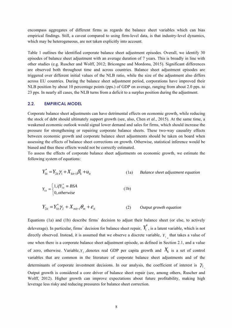
2.2. EMPIRICAL MODEL

herwise, statistical inference would be

te balance sheet adjustments on economic growth, we estimate the llowing system of equations:

itkkititit −1121 (1a) Balance sheet adjustment equation

otherwise,0 (1b)

itmmititit −1212 (2) Output growth equation

w Table 1 outlines the identified corporate balance sheet adjustment episodes. Overall, we identify 30 episodes of balance sheet adjustment with an average duration of 7 years. This is broadly in line with other studies (e.g. Ruscher and Wolff, 2012; Bricongne and Mordonu, 2015). Significant differences are observed both throughout time and across countries. Balance sheet adjustment episodes are triggered over different initial values of the NLB ratio, while the size of the adjustment also differs across EU countries. During the balance sheet adjustment period, corporations have improved their NLB position by about 10 percentage points (pps.) of GDP on average, ranging from about 2.0 pps.

Corporate balance sheet adjustments can have detrimental effects on economic growth, while reducing the stock of debt should ultimately support growth (see, also, Chen et al., 2015). At the same time, a weakened economic outlook would signal lower demand and sales for firms, which should increase the pressure for strengthening or repairing corporate balance sheets. These two-way causality effects between economic growth and corporate balance sheet adjustments should be taken on board when assessing the effects of balance sheet corrections on growth. Otbiased and thus these effects would not be correctly estimated. To assess the effects of corporafo

uXY ++= βγ*Y

≡

=BSAifY

Y itit

,1 *1

1

XY εθγ ++= *Y

Equations (1a) and (1b) describe firms` decision to adjust their balance sheet (or else, to actively

deleverage). In particular, firms` decision for balance sheet repair, *

1Y , is a latent variable, which is not

directly observed. Instead, it is assumed that we observe a discrete variable, 1Y , that takes a value of

one when there is a corporate balance sheet adjustment episode, as defined in S tion 2.1, and a value

of zero, otherwise. Variable,2Y ,denotes real GDP per capita growth and kX is a set of control

variables that are common in the literature of corporate balance sheet adjustments and of

determinants of corporate investment decisions. In our analysis, the coefficient of interest is 1

ec

the

γ . Output growth is considered a core driver of balance sheet repair (see, among others, Ruscher and Wolff, 2012). Higher growth can improve expectations about future profitability, making high

verage less risky and reducing pressures for balance sheet correction. le

8

Also, the decision of firms to adjust their balance sheet can be affected by several other factors. A prominent determinant of balance sheet adjustments is debt overhang. High levels of outstanding debt can have a dampening effect on corporate investment spending, notably via affecting corporates` benefit of investing (Occhino and Pescatori, 2010). In particular, equity holders have less incentives to undertake new investment projects, even in the case of profitable investment opportunities, given that any increase in the firm`s value will be used for repaying debt and will not accrue to equity (see, also, Kalemli-Özcan et al., 2015). In the presence of financial frictions, a high stock of corporate debt can also raise the cost of capital and discourage new investment projects. Although hardly stressed in the relevant literature, the debt overhang effect is also associated with the savings channel. A high stock of corporate debt can induce firms to reduce recruitment expenses and spending on wages, leading to increased corporate savings (Occhino, 2010). In this analysis, debt overhang is proxied by the ratio of total debt-to-gross operating surplus.5 It is noted that recent empirical evidence supports the presence of important interlinkages between corporate and household debt (Bricongne and Mordonu, 2015); this ould lead to a varying impact of the stock of corporate debt on firms` balance sheets and output

e, that can drive increased foreign sales and thus support orporate balance sheet repair.9 Explanatory variables enter the model in a lagged form which should

cgrowth, which we also assess empirically. Following the relevant literature (see, e.g. Ruscher and Wolff, 2012; Goretti and Souto, 2013; Kalemli-Özcan et al., 2015), equation (1a) also includes the following variables: (i) corporate debt maturity, defined as the ratio of long term debt to total debt, to control for the propagation of debt overhang via high ratios of long term debt,6 (ii) corporate liquidity, proxied by the ratio of currency and deposits to corporate value added, to capture the ability of firms to generate cash flows, (iii) credit growth to corporates, to account for external financing conditions, (iv) the ratio of financial net worth to total financial assets, to control for initial balance sheet conditions but also for the presence of financial constraints,7 (v) a systemic banking crisis dummy8, and (vi) competitiveness gains, signalled by changes in the real effective exchange ratcmitigate potential reverse causality issues.

5Several proxies are often used in the literature to define corporate debt overhang. Compared to corporate leverage which is often defined as a percentage of nominal GDP, the debt overhang should be defined in terms of the ability of firms to generate cash flows and service their debt (see, also, Cuerpo et al., 2013). 6According to Myers (1977), short term debt reduces the debt overhang effect due to earlier repayment compared to long term debt, and to less benefits stemming from an immediate investment. By contrast, Diamond and He (2014) find that the timing of investment decisions, debt maturity and firm`s existing assets are important when assessing the debt overhang effect. Short term debt can be associated with higher rollover risk, especially during downturns, and more volatile equity values and thereby, more volatile debt overhang, which can affect future investment projects. 7A more appropriate proxy of balance sheet strength would be the ratio of net worth to total assets. Net worth-to-total assets ratio includes both financial and non-financial assets, and liabilities. However, due to lack of data for non-financial assets of non-financial corporations, we employ financial net worth which is the difference between financial assets and financial liabilities. 8Data is taken from the systemic banking crises database of Laeven and Valencia (2012). A banking crisis is defined as systemic when there are significant signs of financial distress in the banking sector as well as policy intervention measures in response to significant losses in the banking sector (for details, see Laeven an Valencia, 2012). 9Corporate taxes could be another potential determinant of corporate balance sheet repair. For instance, case studies have shown that non-financial corporations` balance sheet adjustment in Germany was largely affected by the tax reform in 2001 (see, Ruscher and Wolff, 2012). However, the inclusion of the change in corporate taxes in preliminary estimations results in statistically insignificant coefficient. This can be due to the very short annual data series (both in terms of time and country coverage) available on corporate taxes which also implies little variability over time. At the same time, corporate taxes may not exercise a direct impact on corporate balance sheets in the sense that what matters for corporates is the effective tax rate. The latter depends inter alia on the state and composition of firms` balance sheet.

9

Equation (2) describes output growth equation. Here, the balance sheet adjustment variable,1Y ,

enters as an explanatory variable and denotes the decision of corporates to repair their balance sheets.

The control variables, mX , included in the growth equation, are: (i) corporate debt overhang, proxied

by the ratio of total debt-to-gross operating surplus, (ii) world GDP per capita growth, (iii) discretionary fiscal policy actions, proxied by the cyclically-adjusted primary budget balance to GDP ratio, (iv) the change in the real short-term interest rate, (v) competitiveness in terms of unit labour costs, captured by the real effective exchange rate, (vi) changes in real asset prices, to account for wealth and profitability effects in the household and corporate sector respectively, and (vii) a set of year dummies to cont

the

rol formo

ods. In

the economic crisis in 2008-2009 and the "double dip" recession in the EU 2012-2013. Again, st variables are lagged once to control for potential reverse causality issues

particular, we consider a vector of instruments, njZ

in(see, also, Table 2). As already discussed, if the decision of firms to repair their balance sheet depends also on current real GDP growth, then balance sheet adjustments (i.e. variable

1Y ) and GDP growth (i.e. variable 2Y ) are

endogenous. Estimates of the effects of balance sheet corrections on GDP growth (equation 2) without controlling for this endogeneity will be biased. To address this issue, we solve t system described by equations (1) and (2), and estimate the derived reduced form parameters by using instrumental variable

(IV) estimation meth

he

&& , that can be used to

redict the endogeno ressor in each equation, where j=1,2 is the number of equations in the system

he system.10 An instrumental variable should be ) relevant, namely it should be correlated with the endogenous variable, and (ii) it should be valid,

GMM") test to assess whether the

p us reg

itv

, as follows:

nit ZY += 11&&ξ (3)

itnit ZY ωπ += 22&& (4)

Equations (1) and (2) are estimated separately by using a limited-information estimation approach (see, among others, Greene, 2000). Compared to the simultaneous system estimation (or full information approach), our method has the benefit of computational simplicity but also that otentmisspecification of one equation does not feed into the other equations of the system. The identification approach is to use as (excluded) instruments of the endogenous variables (i.e.

1Y and 2Y

) a sub-set of the exogenous explanatory variables in t

p ial

(inamely it should remain orthogonal to the error term. Against this backdrop, the instrument set for each of the two endogenous regressors is selected as follows: First, we use an LM test to assess the instruments for potential redundancy, namely for non-correlation with the relevant endogenous regressors (see, also Breusch et al., 1999). If a set of instruments is redundant, then the large-sample efficiency of the model estimation is weakened. Also, increasing the number of instruments does not always improve the estimation efficiency and can lead to poor finite-sample performance. In effect, for the selected instruments, Znj, the null that the correlation with the endogenous regressor is zero, could not be accepted, suggesting that the instruments are not redundant. Second, we use a C (or "distance

10Excluded instruments are exogenous variables that do not enter the equation to be estimated, but are included in the other equations of the system. First stage regressions are reduced form regressions of the endogenous variables both on the (excluded) instruments and the exogenous variables included in the equation to be estimated (see, also, Baum et al., 2003).

10

instruments are exogenous (i.e. if the orthogonality conditions are met) (see, Baum et al., 2007).

growth equation, the ecision of firms to correct their balance sheet is instrumented by a set of balance sheet variables,

rbances. Notwithstanding, the caveat for employing a linear probability model is that the estimated coefficients may not be bounded within the [0,1] interval,

tative.

rowth for a panel of 25 EU Member States over the period 1995-2015, by using strumental variable (IV) estimators. Data definitions and sources are provided in Section A of the

estimated models are not under-identified and the use of IV estimators is justified. The tter in particular suggests that corporate balance sheet adjustments and output growth are

neous effects between utput growth and balance sheet corrections. In that regard, the FE estimator assumes that GDP growth

Again, the selected instruments meet the exogeneity requirement. Following this approach, in the balance sheet adjustment equation, output growth is instrumented by world GDP growth, a set of time dummies that capture the economic crisis and the "double dip" recession in the EU and the lagged cyclically adjusted primary balance. In the dnamely the ratios of long term debt to total debt and financial net worth to assets. Finally, it should be noted that while firm`s decision to deleverage, namely the dependent variable in equation (1), is a binary variable, we follow Angrist (2001) and Angrist and Pischke (2009) and use a linear estimation approach of the balance sheet adjustment equation, instead of using standard probit or logit models. In our case of a panel setting with endogenous regressors, the merits of this approach are threefold: first, we circumvent the "forbidden regression" problem (see, Angrist and Pischke, 2009). The latter suggests that two-stage least squares (2SLS) should not be applied directly to nonlinear models (e.g. probit models) with endogenous regressors. Second, we can control for unobserved heterogeneity across countries by using a fixed effects IV estimator. By contrast, the fixed effects probit estimator faces the "incidental parameters problem", which results in biased and inconsistent estimates (see, among others, Lancaster, 2000). Third, we can (and should) relax the assumption of homoscedastic and non-autocorrelated distu

which makes the analysis mainly quali

2.3. ECONOMETRIC RESULTS

We assess empirically the determinants of corporate balance sheet adjustments and their effects on economic ginAppendix. Table 2 reports the econometric estimates. At the end of Table 2, we report a battery of statistical tests (see, Section B of the Appendix for an analytical discussion). These confirm that the instruments used are relevant, thelaendogenous.11 Columns (1) and (2) present the fixed effects OLS (FE-OLS) estimates for the corporate balance sheet adjustment and the GDP growth equation, respectively. These are obtained by estimating the two equations separately, without taking into account the potential contemporaohas an impact on firms` decision to repair their balance sheet only with a lag.12

11It should be noted that when endogeneity is rejected but IV estimation techniques are employed, there is loss in terms of efficiency in the estimation (i.e. the asymptotic variance of the IV estimator is large). However, using OLS when endogeneity

the system described by equations (1) and (2) becomes a triangular system of equations and can be estimated

is present should imply a greater loss, namely in terms of consistency. 12In this case,consistently.

11

We first discuss the determinants of corporate balance sheet adjustments.13 Explanatory variables have the expected signs. Assuming a lagged effect of growth on corporate deleveraging in the FE-OLS model, economic growth does not seem to play a role in determining the likelihood of observing a corporate balance sheet adjustment. The growth coefficient has the expected negative sign, indicating that lower growth makes it more likely that firms repair their balance sheets, but it is statistically insignificant. By contrast, we find a significant role of debt overhang in determining balance sheet corrections. An increase in the stock of debt is associated with a higher likelihood that firms cut investment spending and/or increase corporate savings to improve their balance sheets. Under the FE-OLS estimates, evidence that the debt overhang effect works on average via long term debt is weak. The higher the ratio of long term debt to total debt is, the higher the dis-incentives to invest, and

erefore the pressure on corporate balance sheets and the need to deleverage. Controls of debt

ate deleveraging. Yet, the effect is not statistical ignificant. Similarly, we do not find a significant impact on corporate balance sheet adjustment from

thmaturity however are statistically significant only at the 10% level. Our estimates suggest that firms` deleveraging decisions are affected by their net financial position. A higher financial net worth to assets ratio is positively associated with the likelihood of observing a persistent improvement in corporate balance sheets in subsequent years. This could imply that on average firms use an improved financial position to repair their balance sheet and reduce the stock of debt. From an alternative perspective, the positive impact of financial net worth on firms` deleveraging suggests that there is little evidence over the binding role of financial frictions in the EU on average.14 For instance, firms with a lower net financial to assets ratio can still on average increase investment spending and/or lower corporate savings, implying some dependence on sources of external funding.15 Also, we find a strong role of liquidity in the non-financial corporate sector for balance sheet repair. Lower corporate liquidity makes it more likely that firms adjust their balance sheets by increasing savings, notably lowering operating costs, and/or by reducing corporate investment. This finding is in line with case studies on historical deleveraging episodes (see, for instance, Ruscher and Wolff, 2012; Goretti and Souto; 2013). The bank lending channel has also an important effect on corporate deleveraging. Our estimates suggest that firms are more likely to repair their balance sheets under tighter credit conditions. Banking sector restructuring or deleveraging may well result in increased borrowing rates for corporates and lower credit growth. On the remaining control variables, the coefficient of systemic banking crises has the appropriate sign suggesting that banking distress is associated with a higher likelihood of corporscompetitiveness gains and higher foreign sales. Turning to the growth equation, FE-OLS estimates suggest that firms` decision to repair their balance sheet has a negative impact on GDP growth. However, assuming no controls for the contemporaneous interaction between growth and deleveraging, the effect of balance sheet repair on growth is not

13Given the caveat discussed in Section 2.2 of the linear probability model, our discussion remains mainly qualitative. 14This finding should be treated with caution given that it may mask differences at the Member-State level. For instance, the sample correlation of financial net worth-to-assets ratio with corporate deleveraging is negative for some EU countries, such as ES, PT, EL, CY etc. where financial frictions could weigh on investment activity. We repeated the estimation of the balance sheet adjustment equation for this subset of countries. Indeed, the sign of financial net worth to assets ratio turns now negative, suggesting that higher financial net worth is associated with higher corporate investment and/or lower savings, probably reflecting financial constraints. 15Lower net worth (i.e. an increase in leverage) has been found to have a positive impact on corporate investment during normal times in the euro area (see, Kalemli-Özcan et al., 2015). Access to external funding should however depend on the business sector but also on firms` size. Small and medium sized firms could face tighter credit conditions and lower ability to tap the markets compared to large corporates. At the same time, some sectors, like for instance the construction sector, rely more on bank lending compared to other sectors (e.g. services).

12

statistically significant. By contrast, our estimates suggest that tackling the crisis legacies, such as the high stock of corporate debt, should support GDP growth. More specifically, a 20 percentage points decline in the corporate debt ratio is associated with 10 basis points increase on average in annual real GDP growth. As for the other control variables, the coefficient on world GDP growth is positive and highly significant. Also, higher discretionary fiscal effort, which is proxied by the level of the cyclically adjusted primary budget balance, seems to have positive impacts on economic growth. Although this finding largely supports the view of positive short run effects from improving fiscal imbalances, it should be interpreted with caution given that it can be attributed to the way in which the discretionary fiscal stance is measured (see, also Guajardo et al., 2011).16 The negative coefficient of changes in the real short term interest rate suggests that an accommodative monetary policy is ssociated with higher growth, though the effects are not statistically significant. 17 Lastly, favourable

cts between growth and deleveraging underestimates the impact of demand pressures n corporate balance sheet corrections. Adverse demand pressures will tend to worsen firms` and

term debt, is the main channel of debt overhang effects on corporate balance sheets. n the remaining variables, the results are broadly in line with FE-OLS estimates. For instance, lower

areal asset price movements and cost competitiveness gains are associated on average with higher output growth. Columns (3) and (4) show the instrumental variable (IV) estimates. More specifically, we report the 2-step GMM estimates which take on board the contemporaneous effects between growth and corporate deleveraging.18 Results in column (3) show that GDP growth has now a strong negative statistical effect on corporate balance sheet corrections. This suggests that failing to control for simultaneity effeoconsumers` expectations, making high leverage more risky and increase the need for repairing firms` balance sheets. Based on the estimates in column (3), the coefficient of current growth is statistically significant, yet high economic growth is not the sole driver of firms` deleveraging decisions. Corporate balance sheet variables have broadly the same effect on corporate balance sheet adjustments as FE-OLS estimates in column (1). Our findings therefore suggest that high debt overhang weighs on corporate balance sheets and pushes firms on a deleveraging mode. Also, the coefficient of long term debt to total debt ratio is now highly statistically significant. This clearly supports the view that the maturity of debt, and in particular, longOcorporate liquidity and credit growth are associated with a higher likelihood of firms switching to deleveraging.

16There is little consensus in the literature on the expansionary effects of fiscal consolidation. The Alesina and Ardagna (2010) traditional approach of using the cyclically adjusted primary balance to define fiscal adjustment episodes has been criticised on the back of increasing the bias in favor of expansionary fiscal adjustments. Cyclically-adjusted fiscal variables can be influenced by changes unrelated to discretionary fiscal actions, such as changes in asset prices or other temporary factors (i.e. one-offs, classification errors etc.). Despite the caveats, this approach is the most commonly used. 17The lack of statistical significance of the effects of monetary policy on growth could be attributed to the timing of the impacts assumed by the model, namely the use of the lagged (change in the) real short term interest rate. The latter is in line with the literature on the transmission of monetary policy to the economy. In particular, empirical studies substantiate that the full pass-through of changes in monetary policy on real GDP ranges between four and six quarters in the euro area (ECB, 2000, 2010). Still, we repeated the estimations, assuming a contemporaneous, rather than lagged, impact of changes in the short term interest rate. The coefficient is still negative but turns statistically significant, while the remaining findings, which are the focus of the analysis, are unchanged. 18Conventional IV estimators, such as two-stage least squares (2SLS) are special cases of this IV-GMM estimator. The advantage of the 2-step GMM estimator is that it is more efficient than standard IV/2SLS estimators in the presence of heteroskedasticity. Our estimates are based on heteroskedasticity- and autocorrelation-consistent (HAC) standard errors. These are obtained by using the Newey and West (1987) Bartlett kernel function with the kernel function`s bandwidth set to T1/3, where T is the number of time periods. Given our unbalanced panel, we set the bandwidth equal to 2.

13

Column (4) presents the 2-step GMM estimates for the growth equation. The effect of corporate deleveraging on growth is negative and, in contrast to the FE-OLS estimates, is statistically significant. The estimates suggest that a shift of corporates` to a deleveraging mode decreases output growth by 1.8 percentage points compared to a period when no deleveraging takes place. This finding is in line with the view that balance sheet correction comes with a cost in terms of output loss at least in the short run (see, also Chen et al., 2015). Considering that the average duration of a deleveraging episode is 7 years on average in the EU sample, the average impact on annual output growth would be about 20 basis points. Moreover, reducing the stock of corporate debt is associated on average with higher

rporate and household debt mainly via the wage channel (see, Bricongne and ordonu, 2015). Highly indebted households will tend to get less credit and consumption which

al GDP growth by 10 basis points on average. In turn, correcting corporate balance sheets during periods of

ousehold sector increases the pressure for household deleveraging and should have some costs in terms of growth, reducing the overall benefit for the economy.

e assess the robustness of the empirical findings by performing a set of alternative estimations.

growth. The overall impact is now somewhat lower than discussed above; specifically, a 20 percentage points decline in the corporate debt ratio is associated with 6 basis points increase on average in annual real GDP growth. Estimates for the remaining variables are similar to the FE-OLS estimates. So far, our results suggest that debt overhang is an important driver of firms` decision to correct their balance sheet. Still, the stock of corporate debt can have a stronger impact on firms` balance sheets but also on output growth if there are other indebted sectors, such as the household sector, in the economy (Bornhorst and Ruiz-Arranz, 2013). Recent empirical evidence substantiates the interlinkages between non-financial coMshould in turn impact on demand and profitability prospects for corporates and weigh on corporate balance sheets. Columns (5) and (6) show the 2-step GMM estimates for the two equations, now adding a dummy variable capturing household indebtedness and its interaction with corporate debt overhang.19 In particular, the dummy takes a value of 1 when the household debt-to-income ratio at time t is higher than the respective country-specific sample mean, and 0 otherwise. Estimates in column (5) suggest that higher debt overhang weighs more heavily on corporate balance sheets and can trigger balance sheet corrections during periods when household debt overhang is high. As regards growth, column (6) shows that a decrease in the stock of corporate debt is more beneficial for growth during periods of lower household debt.20More specifically, a 20 percentage points decline in the corporate debt ratio during periods when household debt is below the country-specific average boosts annual re

relatively high indebtedness of the h

2.4. ROBUSTNESS CHECKS

WTables 3 and 4 present the robustness checks. Again, the statistical tests on the IV estimators reported at the end of the Table 3 suggest that all models are well specified. More specifically, we first assess the robustness of the baseline results in the case of weak instruments. As already discussed in Section 2.2, weak instruments can lead to biased IV/2SLS estimates. In order

19The (exogenous) threshold dummy allows to partly capture nonlinear effects amid a state of higher/lower household debt (compared to average linear impacts captured by a household debt overhang covariate). 20Equivalently, the results can be read as suggesting that a rise in corporate debt overhang is slightly less detrimental for growth at a state where household indebtedness is relatively higher. Although, this is somewhat counter-intuitive, it can be read in the context of the consumption smoothing effects of household debt, which are commonly larger for credit-constrained households. In particular, higher household debt has been often associated with a consumption boom in the short run, whereas correcting an accumulated high stock of debt is more painful for the economy (see, among others, Mian et al., 2015; Lombardi et al., 2017)

14

to control for any remaining weak instruments bias, we estimate the baseline speciation (columns (3) and (4) of Table 2) by applying the Continuous Updating Estimator (CUE) proposed by Hansen et al. (1996). The CUE estimator has been found to perform better than the 2-step GMM estimator under the presence of weak instruments (Hahn et al., 2004). CUE estimates are presented in columns (1) and (2) of Table 3. These confirm our previous findings. More specifically, the decision of corporates to eleverage has a negative and statistically significant impact on economic growth. At the same time,

the likelihood that firms correct their balance sheets, but the coefficient is now only eakly statistically significant. At the same time, the coefficient on systemic banking crises turns

fied.22 Columns (5) and (6) present the results. The point estimates of the oefficient on growth and the decision to deleverage are very similar to those in Table 2. By contrast,

which could in turn be correlated with firms` decision to repair their balance sheet. Such an effect

deconomic growth but also balance sheet variables play an important role in determining corporate balance sheet adjustments. As a second robustness check, we use an alternative definition of corporate deleveraging episodes. To this end, we define balance sheet adjustment episodes as set out in Ruscher and Wolff (2012); namely, we do not account for country-specific adjustments in the NLB position, but instead we take on board a uniform improvement criterion of the NLB position (by 2.0% of GDP) for all economies (see, Section 2.1). Columns (3) and (4) of Table 3 present the 2-step GMM estimates for this alternative definition of corporate balance sheet adjustments. The findings are in line with the benchmark estimation results. Corporate balance sheet adjustments have a dampening effect on growth and balance sheet variables decisively determine firms` decision to deleverage. A favourable economic outlook weakenswsignificant, suggesting that corporate balance sheet adjustments are more likely in the aftermath of a financial crisis. An additional robustness check concerns estimating a parsimonious model specification for capturing corporate balance sheet adjustments (i.e. equation (1)). The reasons are twofold; first, including a large set of balance sheet variables as determinants of balance sheet adjustments could induce some collinearity effects in the baseline estimations.21 Second, the first stage F-statistic for the growth baseline model is slightly higher than 10, which is the Staiger and Stock (1997) threshold for judging against model under-identification. Using a parsimonious specification on balance sheet adjustments would imply a lower number of instruments used in the growth equation, which can have the advantage of minimising weak instruments bias (Angrist and Pischke, 2009). In that regard, we perform the estimations by including only debt overhang and financial net worth as balance sheet variables in the balance sheet adjustment equation. The decision of firms to adjust their balance sheet is therefore instrumented only by the ratio of financial net worth to assets, which implies that the equation is exactly identiclowering the stock of corporate debt has a smaller positive impact on growth, and the effect is weakly statistically significant. A final robustness check is to assess the instrument validity of the fiscal balance in the corporate balance sheet adjustment equation. More specifically, our identification strategy is based on the fact that the instruments are correlated with output growth, which is the instrumented variable in the balance sheet equation; the (lagged) cyclically adjusted primary balance should have an impact on output growth. However, the lagged fiscal balance could induce changes in future corporate taxation

21 Still, the pairwise correlations of the corporate balance sheet variables are well below 0.5. 22In exactly identified models, Hansen`s J statistic that formally tests the exclusion restrictions on the instruments cannot be computed.

15

would invalidate our instrument. To address this concern, we empirically examine whether the lagged cyclically adjusted primary balance ratio has an impact on corporate taxes.23 Table 4 reports the results

om this exercise, where we find an insignificant, close to zero, effect of our instrument on corporate taxes.

3.

c stochastic general equilibrium (DSGE) model developed y the European Commission (see Ratto et al., 2009; Roeger and in 't Veld, 2010, for a detailed

us tightening in the collateral constraint of non-financial firms. Although in principle financial intermediaries can

mium to the loan rate that reflects corporate firms' safety and borrowing capacity, an analysis of the reduction in debt-overhang is not investigated in this context.

h a tightening of the entrepreneurs' collateral constraint, ading to a reduction in loans and adversely affecting investment and growth in the short-run. In what

share of loans in the balance sheet of ntrepreneurs is ensured by assuming that they have a higher rate of time preference. In this case

of entrepreneurs requires that banks restrict lending by imposing a collateral constraint. This pecification closely follows Kiyotaki and Moore (1997).

guments. Savers can hold

fr

CORPORATE DELEVERAGING AND MACROECONOMIC ADJUSTMENT

In order to understand the dynamic aspects of corporate deleveraging, we subsequently employ a banking variant of the Commission's QUEST model. We modify a closed economy version of QUEST to assess the impact of corporate sector deleveraging on the main macroeconomic aggregates. QUEST is an open economy new-Keynesian dynamibdescription of the model)24, and incorporating various empirically-relevant real, nominal as well as financial frictions, used for policy analysis. The model is able to investigate the impact of corporate deleveraging through an exogeno

attach an endogenous risk-pre

3.1. MODEL OUTLINE

The QUEST variant used in this study is a closed economy model calibrated to the EU aggregate economy, which incorporates a banking sector with bank capital. We opt for this model variant as it distinguishes the household sector into savers and borrowers (entrepreneurs). Entrepreneurs finance their investment decisions by taking out loans from the banking sector subject to a collateral constraint. Corporate deleveraging can be triggered througlefollows we only outline the main features of the model and direct the interested reader to Roeger (2014) for a more detailed model description. In order to allow for a meaningful financial intermediation function of banks, the household sector is disaggregated into savers and borrowers. A positive esolvency s Savers: We follow van den Heuvel (2008) and assume that savers maximise an intertemporal utility function with consumption, liquidity services provided by deposits and leisure as ar

23See, also Kitsios and Patnam (2016) for a similar approach. 24For references to QUEST model publications see: https://ec.europa.eu/info/business-economy-euro/economic-and-fiscal-policy-coordination/economic-research/macroeconomic-models_en

16

wealth either in the form of government bonds, bank deposits or bank equity and receive interest come from bonds and deposits and dividends. Savers require an equity premium on bank stocks.

ntrepreneurs (borrowers) maximise an intertemporal utility function over entrepreneurial

ver distributed profits which they use for consumption. At the beginning of each period, the

vestment and labour demand decisions. Firms partly finance investment by king out loans from the banking sector. To prevent over borrowing, banks impose a collateral

inSavers also offer labour services to entrepreneurs and receive wage income. Entrepreneurs: Econsumption, subject to a budget constraint, a capital accumulation constraint and a collateral constraint. They make pricing, labour demand, investment and financing decisions and use a Cobb-Douglas production function. The continuum of entrepreneurs is distributed over a unit interval )1,0(∈i . Entrepreneur i uses a

constant returns to scale technology to produce goods which are imperfect substitutes for goods produced by its competitors and we assume monopolistic competition. In addition we assume that price changes are subject to adjustment costs. En epreneurs maximise an intertemporal utility functiontroentrepreneur makes intaconstraint by restricting loan supply to fraction ξ of the value of the capital stock (see equation (5)).

al constraint

ks that the ratio of deposits loans should not exceed a certain target ratio. Concerning liquidity requirements, banks are asked to

share of loans. This imposes an opportunity cost for banks since liquid ssets (government bonds and assets) yield a lower return. Banks can increase capital either by issuing

onetary and fiscal policy:

he central bank follows a Taylor rule. Fiscal policy is constrained by a budget constraint. overnment debt is held by saver households and banks (for liquidity purposes).

raph 1 below schematically summarises the economic linkages in the model.

Collater (1 ) (1 )L K

t it t itr L q Kξ δ+ = − (5)

Banks: Banks provide loans to entrepreneurs and demand deposits from saver households. They maximise the present discounted value of dividends or the stock market value of the bank subject to a capital and liquidity requirement constraint. The capital requirement demands from bantohold liquid assets as a fixedanew shares or via retained earnings. Both strategies yield identical results. M TG G

17

Graph 1: Model Overview

t on e underlying dynamics of the main macroeconomic aggregates over time. In order to explore the

tylised scenario: A tightening of entrepreneurs’ collateral constraint calibrated to generate a 2%

ters are calibrated according to Roeger (2014), who studies changes in gulatory requirements in the banking sector, whereas parameters for the non-financial sector are

ffects domestic demand and in particular onsumption (distributed profits) and investment. The effects of the collateral constraint shock can be

ons (6) and (7) below.

3.2. SIMULATIONS

The main result of the empirical analysis of Section 2 yielded inter alia two central results: i) that periods of active corporate deleveraging are associated on average with lower output growth compared to periods when no adjustment takes place, and ii) a decline in the corporate debt ratio25 seems to be associated with an increase on average in annual real GDP growth. While the IV estimation lets the “data speak”, arguably, it only captures an average effect over the sample and does not shed lighthchannels through which deleveraging affects growth we simulate the following stylised scenario. Spermanent reduction in loans, phased in over 3 years. Recall that the model employed incorporates a rich financial sector with a meaningful financial intermediation function for banks. As such parameters can be categorised into financial and non-financial. Financial parameretaken from Ratto et al. (2009). A tightening in entrepreneurs’ collateral constraints acillustrated by observing the equati Consumption of entrepreneurs

))1(1( Lt

Eit r+−

=ψ

)1( ELE rC + β1 t

Eit

it

C+ (6)

25Defined as debt divided by gross operating surplus.

Consumers(Housholds)

Central Bank

Entrepreneurs(Firms)

Banks

Labour

Deposits

Bank equity

Loans Government

Taxes

Bonds

Consumptiongoods Labour

Cash

18

Eitψ : Lagrange Multiplier of Collateral constraint

Investment

)1(, ξψδ −++= Eit

LtitK rY (7)

Equation (6) is the entrepreneur’s Euler equation equating the marginal utility of current and future consumption (scaled by the relative price between the two), whereas Equation (7) is the entreprene

optimality condition for investment. A tightening of the collateral constraint (decrease in

ur’s

ξ in equation

(2)) implies that the Lagrange multiplier associated with this constraint (Etψ ) becomes positive.

Etψ

cts like a risk premium to the interest rate of entrepreneurs. Froma equations (6) and (7) it is thus clear

in consumption and investment is not symmetric with consumption

that an increase in the Lagrange multipliers increases the the loan rate incentivising entrepreneurs to increase savings and lower their consumption and investment. Table A plots the responses of the main macroeconomic aggregates for the scenario specified above. As can be seen a shock to the collateral constraint triggering a 2% reduction in the stock of loans over 3 years brings down consumption and investment on impact and translates to a reduction in real GDP

the short run. The reduction indeclining by 0.1% and investment falling by 0.4% on impact. Overall, this suggests a decline in real GDP of 0.14% in the first year. The tightening of the collateral constraint and the reduction in investment and consumption also has

implications for corporate debt. While the constraint is tight (Etψ positive) and the loan rate is still

high, entrepreneurs reduce their stock of corporate debt (corporate debt as a share of GDP declines by pproximately 3% in year 2). At the same time, the model also features an endogenous ama plification

tion is seen to fall by 0.13p.p on impact. But, as

ption picking up. As can be seen in year 25 total

stock market. Whilst the stock of loans and corporate debt is decreased, capital is increased by 0.05%

mechanism. As can be seen from Equation (7) as investment falls, the collateral constraint tightens further causing corporate debt to continue falling (approximately 7% in year 3 onwards). The reduction in domestic demand in the short run also brings down prices and can hence slow down

e speed of deleveraging in terms of loans. Inflathfalling prices also reduce the value of capital, this leads the collateral constraint to tighten further and the corporate sector to deleverage more strongly. In the medium to long run, once corporate debt has been reduced the effects fade away and the conomy recovers with investment and consume

consumption is up by 0.07% whereas investment is higher by 0.05%. This translates to largely neutral, effects on growth with GDP up by 0.02%. There are two effects at work: On the one hand, the reduction in corporate debt due to deleveraging endogenously loosens the collateral constraint (the Lagrange multiplier becomes negative). As the deleveraging shock is phased in, the risk premium on the loan rate also declines. As the loan rate starts falling entrepreneurs may now increase their investment from further bank lending. However, we observe a fall in the stock of loans. This is because bank financing requires a premium over internal financing. As such, entrepreneurs substitute away from bank financing and into financing from the

19

in the long run. Given the neutral effects in the long run it can be concluded that the source of investment financing, be it financial intermediaries or the stock market, does not seem to matter much

r long run GDP.

are of GDP stemming from increased tax revenues on the consumption and capital income ases.

Table A: Responses of macroeconomic aggregates

otes: QUEST simulations. Results are reported as deviations from a no-shock baseline.

ere are additional channels through which corporate deleveraging can affect output more enerally.

uld capture the positive ffects that a reduction in debt overhang would have on economic activity.

Year 1 2 3 4 5 10 25 150Percent

GDP -0.14 -0.02 -0.04 -0.02 -0.01 0.00 0.02 0.02

Investment -0.43 -0.29 -0.01 0.07 0.05 0.07 0.05 0.05

Capital -0.01 -0.02 -0.03 -0.02 -0.02 0.00 0.04 0.05

Cons.total -0.10 0.08 -0.01 0.00 0.01 0.02 0.05 0.07

Cons.saver 0.38 0.14 -0.21 -0.29 -0.25 -0.26 -0.23 -0.22

Cons.entre -0.51 0.02 0.16 0.24 0.24 0.26 0.30 0.31

Stock of loans -0.96 -1.39 -1.95 -1.86 -1.82 -1.84 -1.81 -1.80

Employment -0.23 -0.01 -0.05 -0.02 0.00 0.00 0.00 0.00

Real wages -1.30 -0.04 -0.23 -0.10 -0.02 -0.01 0.01 0.02

Real loan rate -9.12 -29.30 -45.99 0.99 -2.98 -4.38 -4.45 -4.47

Lagrange mult.cc 65.38 118.65 116.28 5.15 -16.46 2.67 2.39 2.36

Percentage points

Corporate debt-to-GDP -0.12 -3.41 -6.62 -6.46 -6.24 -6.43 -6.38 -6.36

Public debt-to-GDP 0.18 -0.73 -1.24 -0.69 0.35 -0.22 0.07 0.00

Nom.int.rate -26.84 -31.60 -11.87 4.23 -0.34 0.53 0.14 0.00

0.00 0.00 0.00

fo The impact on output also has effects for the government budget through the activation of automatic stabilisers. The government budget balance is positively affected in the medium run as public debt falls as a shb

Inflation % -0.14 -0.01 0.06 -0.01 -0.01

N Besides the effects that a tightening of the collateral constraint has on household demand in this exercise, thg In principle, banks can attach an endogenous risk premium to their loan rate reflecting the riskiness of non-financial firms' borrowing capacity. As a non-financial firm engages in deleveraging and its corporate debt declines, thus lowering its financing costs, this can signal to banks that is has also become safer – the burden of debt overhang is lightened. As a result, banks can now endogenously reduce the risk premium attached to their interest rate, allowing for the loan rate to decline more strongly, and firms to engage in additional investment. Such a mechanism woe In addition, a corporate deleveraging shock can be interpreted as a negative shock to savers' expected income causing labour supplied to increase in the long run. This is because the value of the assets held by savers declines following the deleveraging shock. At the same time however, labour demanded by entrepreneurs also falls. The impact on employment in equilibrium significantly depends on the degree of wage flexibility and the strength of the wealth effect saver households are experiencing. In the short run a fall in wages would be contained and employment would decline. In the long run however, as

20

saver households reduce their consumption, this may boost labour supplied and employment. This would be an additional channel through which GDP can increase. In this exercise however, we assume a specification of the intratemporal labour supply equation such that the savers' wealth effect is absent.

s such, despite an increase in their consumption in the long run labour supply remains constant.

ted with an increase in net savings either through lower investment, higher savings or oth. This is commonly expected to have a more detrimental impact on growth compared to passive

nd, as repairs in firms` balance heets are accompanied by output losses, our econometric work further illustrates that reductions in

picks up allowing the economy to recover. In the long run, the source of investment financing, e it banks or the stock market, does not seem to matter much for GDP, with the effects being largely

nditions, caused by negative demand or supply shocks. Moreover, a systematic investigation of banks' objective functions would allow capturing additional channels of corporate deleveraging shocks.

A

4. CONCLUSION A legacy of the recent crisis is the excessive stock of private sector debt, including high levels of corporate debt, in some European economies. Active deleveraging in the non- financial corporate sector is associabdeleveraging. We have used an econometric approach to quantitatively investigate the effects of corporate balance sheet adjustments on economic growth in the EU by modelling the ability of the non-financial corporate sector to correct its balance sheet and a growth equation in an instrumental variables (IV) panel context. The novelty of the approach has been that it enabled us to consider the contemporaneous effects between corporate balance sheet adjustment and economic growth, which can otherwise lead to biased estimates. Our results indicate that periods of active corporate deleveraging are associated on average with lower output growth. On the other hascorporate debt overhang are associated with higher economic growth. Our model-based simulations have explored a possible mechanism for the econometric findings on the effects of corporate balance sheet adjustment on output growth in the EU. In particular, we have shown, that following a corporate deleveraging shock, which reduces the stock of loans, investment, consumption and GDP decline in the short-run. In the medium-run, however, as the corporate debt burden lightens and entrepreneurs substitute away from bank financing of their investment, domestic demand bneutral. Finally, our analysis can be extended along several dimensions. First, we do not account for the presence of non-linearities. It could be, for instance, that corporates` balance sheet reaction to a growth shock is not linear, but depends on the sign and the magnitude of the shock. At the same time, there may be a threshold when debt overhang becomes a problem for corporate balance sheets but also for economic growth. On the modelling side, the analysis has abstracted from confounding deleveraging shocks with additional shocks, which may simultaneously hit the economy and lead to adverse effects on the baseline. Interesting avenues of further exploration could study the effects of corporate deleveraging shocks under the presence of adverse economic co

21

REFERENCES

Alesina, A., and S., Ardagna (2010). Large Changes in Fiscal Policy: Taxes versus Spending. Tax Policy and the Economy, Vol. 24, ed. by Jeffrey R. Brown (Cambridge, Massachusetts: National Bureau of Economic Research).

Angrist, D. J., and J.S., Pischke (2009). Mostly harmless econometrics: An empiricist`s companion. Princeton University Press.

Angrist, D.J. (2001). Estimation of limited dependent variable models with dummy endogenous regressors. Journal of Business & Economic Statistics 19(1), pp. 2-28.

Baum, C.F., Schaffer, M.E., and S., Stillman (2003). Instrumental variables and GMM: Estimation and testing. The Stata Journal 3(1), pp.1-31.

Baum, C.F., Schaffer, M.E., and S., Stillman (2007). Enhanced routines for instrumental variables/generalised method of moments estimation and testing. The Stata Journal 7(4), pp. 465-506.

Bornhorst, F., and M., Ruiz-Arranz (2013). Indebtedness and Deleveraging in the Euro Area. Euro Area Policies, 2013 Article IV Consultation Selected Issues, IMF Country Report 13/232.

Breusch, T., Qian, H., Schmidt, P., and D., Wyhowski (1999). Redundancy of moment conditions. Journal of Econometrics 91 (1), pp. 89-111.

Bricongne, J-C., and A.M., Mordonu (2015). Interlinkages between household and corporate debt in advanced economies. European Commission, European Economy Discussion Paper No. 017.

Cecchetti, S.G., Mohanty, M.S., and F., Zampolli (2011). The Real Effects of Debt. BIS Working Papers No. 352 (Basel).

Chen, S., Kim, M., Otte, M.., Wiseman, K.. and A., Zdzienicka (2015). Private sector deleveraging and growth following busts. IMF Working Paper WP/15/35.

Cuerpo, X. Drumond, I., Lendvai, J., Pontuch, P., and R., Raciborski (2013). Indebtedness, deleveraging dynamics and macroeconomic adjustment. European Commission, European Economy Economic Papers No. 477.

Diamond, W.D., and Z., He (2014). A theory of debt maturity: The long and short of debt overhang. The Journal of Finance 69(2), pp. 719-762.

European Central Bank (ECB) (2000). The interest rate transmission mechanism in the euro area: methodologies and an illustration. ECB Monthly Bulletin July 2000.

European Central Bank (ECB) (2010). Monetary policy transmission in the euro area, a decade after the introduction of the euro. ECB Monthly Bulletin May 2010.

Goretti, M. and M., Souto (2013). Macro-financial implications of corporate (de)leveraging in the euro area periphery. IMF Working Paper WP/13/154.

Greene, W., (2000). Econometric analysis. 4th ed. Upper Saddle River, NJ: Prentice-Hall.

22

Guajardo, J., Leigh, D., and A., Pescatori (2011). Expansionary Austerity: New International Evidence. IMF Working Paper WP/11/158.

Hahn, J., and J., Hausman (2002). Note on bias in estimators for simultaneous equation models. Economics Letters 75(2), pp. 237-41.

Hahn, J., Hausman, J., and G., Kuersteiner (2004). Estimation with weak instruments: Accuracy of higher-order bias and MSE approximations. Econometrics Journal 7(1), pp. 272-306.

Hansen, L. (1982). Large sample properties of generalised method of moments estimators. Econometrica 50(3), pp.1029-1054.

Hansen, L., Heaton, J., and A., Yaron (1996). Finite sample properties of some alternative GMM estimators. Journal of Business and Economic Statistics 14(3), pp. 262–280.

Kalemli-Özcan, Ş., Laeven, L., and D. Moreno (2015). Debt Overhang, Rollover Risk and Investment in Europe. (unpublished manuscript).

Kitsios, E., and M. Patnam (2016). Estimating fiscal multipliers with correlated heterogeneity. IMF Working Paper WP/16/13.

Kiyotaki, N., and J. Moore (1997). Credit Cycles. Journal of Political Economy 105(2) (April 1997), pp. 211-248

Kleibergen, F., and R., Paap (2006). Generalised reduced rank tests using the singular value decomposition. Journal of Econometrics 127(1), pp. 97–126.

Laeven, L., and F. Valencia (2012). Systemic Banking Crises Database: An Update. IMF Working Paper WP/12/163.

Lancaster, T. (2000). The incidental parameters problem since 1948. Journal of Econometrics 95(2), pp. 391-413.

Lombardi, M., Mohanty, M., and I., Shim (2017). The real effects of household debt in the short and long run. BIS Working Papers No. 607.

Mian, R. A., Sufi, A., and E., Verner (2015). Household debt and business cycles worldwide. NBER Working Paper No. 21581.

Myers, C.W. (1977). Determinants of corporate borrowing. Journal of Financial Economics 5(2), pp. 147-175.

Newey, W.K., and K.D., West (1987). A simple, positive-definite, heteroskedasticity and autocorrelation consistent covariance matrix. Econometrica 55(3), pp. 703-708.

Occhino, F. (2010). Is debt overhang causing firms to underinvest?. Economic Commentary No. 2010-7.

Occhino, F., and A., Pescatori (2010). Debts overhang in a business cycle model. Federal Reserve Bank of Cleveland Working Paper 10-03R.

Pontuch, P. (2014). Private sector deleveraging: where do we stand? European Commission, Quarterly Report on the Euro Area 13(3), pp. 7-19.

23

Ratto, M., Roeger, W. and J., in ’t Veld (2009). QUEST III: An Estimated Open-Economy DSGE Model of the Euro Area with Fiscal and Monetary Policy. Economic Modelling 26(1), pp. 222-233.

Roeger, W. (2014). Regulatory Measures in the Banking Sector. DG ECFIN, mimeo.

Roeger, W., and J., in 't Veld (2010).Fiscal stimulus and exit strategies in the EU: a model-based analysis. European Economy Economic Papers No. 426.

Ruscher, E., and G., Wolff (2012). Corporate balance sheet adjustment: stylised facts, causes and consequences. European Commission, European Economy Economic Papers No.449.

Staiger, D., and J.H., Stock (1997). Instrumental variables regression with weak instruments. Econometrica 65(3), pp.557-86.

Wooldridge, J.M. (2003). Introductory econometrics. A modern approach. Second edition. NewYork: South-Western College Publishing.

Van den Heuvel, S. (2008). The welfare cost of bank capital requirements. Journal of Monetary Economics 55(2), pp.298–320.

24

25

ECONOMETRIC RESULTS

Table 1:

Year Duration NLB/GDP (t-1) NLB/GDP (T) ΔNLB/GDP(4) (5) (6)=(5)-(4)

2009-2010 2 -0.22 0.01 23.02001-14 14 -0.06 0.03 9.2

1998-2014 17 -0.16 -0.005 15.82010-2014 5 -0.02 0.05 6.62004-2005 2 0.017 0.04 2.22008-2014 7 -0.08 0.015 9.51983-1993 11 -0.06 0.01 7.0

Italy 2012-2015 4 -0.019 0.018 3.7Cyprus 2002-2003 2 -0.05 0.039 9.1Latvia 2009-2014 6 -0.098 0.057 15.6Lithuania 2009-2014 6 -0.052 0.117 16.9Netherlands 2002-2014 13 0.037 0.075 3.8Austria 2002-2004 3 -0.04 0.017 5.7

2009-2014 6 -0.019 0.015 3.4Portugal 2009-2015 7 -0.105 0.006 11.1

2009-2014 6 -0.081 0.037 11.81999-2004 6 -0.077 -0.03 4.72009-2010 2 -0.019 0.01 2.92012-2013 2 -0.014 0.036 5.02009-2010 2 0.006 0.05 4.61996-2002 7 -0.032 0.041 7.32009-2013 5 -0.166 0.043 21.0

Czech Republic 1998-2014 17 -0.074 -0.018 5.6Denmark 2002-2003 2 0.025 0.064 3.9Croatia 2010-2014 5 -0.075 -0.032 4.2

2001-2014 14 -0.07 0.043 11.3Poland 2001-2014 14 -0.067 0.057 12.4

1999-2000 2 -0.20 0.018 22.32002-2007 6 -0.196 -0.046 15.02002-2012 11 -0.05 0.025 7.7

Average duration of episode (years) 7Average change in NLB (in pps. of GDP) 9.4

Belgium

Corporate balance sheet adjustment episodes in the EU

Country

Bulgaria

GermanyEstoniaIrelandGreeceSpainFrance

Slovenia Slovakia

Finland

Notes: For a definit ion of corporate balance sheet adjustment episodes, see Section 2.1. Columns (4)-(6) depict rounded figures.

Hungary

Romania

UK

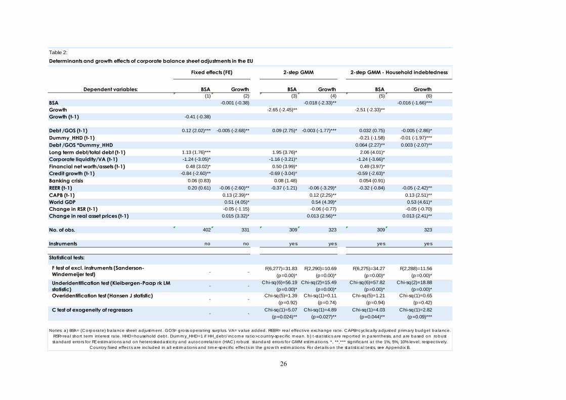
Table 2:

BSA Growth BSA Growth BSA Growth(1) (2) (3) (4) (5) (6)

-0.001 (-0.38) -0.018 (-2.33)** -0.016 (-1.66)***-2.65 (-2.45)** -2.51 (-2.33)**

-0.41 (-0.38)

0.12 (2.02)*** -0.005 (-2.68)** 0.09 (2.75)* -0.003 (-1.77)*** 0.032 (0.75) -0.005 (-2.86)*Dummy_HHD (t-1) -0.21 (-1.58) -0.01 (-1.97)***Debt /GOS *Dummy_HHD 0.064 (2.27)** 0.003 (-2.07)**Long term debt/total debt (t-1) 1.13 (1.76)*** 1.95 (3.76)* 2.06 (4.01)*Corporate liquidity/VA (t-1) -1.24 (-3.05)* -1.16 (-3.21)* -1.24 (-3.66)*Financial net worth/assets (t-1) 0.48 (3.02)* 0.50 (3.99)* 0.49 (3.97)*Credit growth (t-1) -0.84 (-2.60)** -0.69 (-3.04)* -0.59 (-2.63)*Banking crisis 0.06 (0.83) 0.08 (1.48) 0.054 (0.91)REER (t-1) 0.20 (0.61) -0.06 (-2.60)** -0.37 (-1.21) -0.06 (-3.29)* -0.32 (-0.84) -0.05 (-2.42)**CAPB (t-1) 0.13 (2.39)** 0.12 (2.25)** 0.13 (2.51)**World GDP 0.51 (4.05)* 0.54 (4.39)* 0.53 (4.61)*Change in RSR (t-1) -0.05 (-1.15) -0.06 (-0.77) -0.05 (-0.70)Change in real asset prices (t-1) 0.015 (3.32)* 0.013 (2.56)** 0.013 (2.41)**

402 331 309 323 309 323

no no yes yes yes yes

- -F(6,277)=31.83

(p=0.00)*F(2,290)=10.69

(p=0.00)*F(6,275)=34.27

(p=0.00)*F(2,288)=11.56

(p=0.00)*

- -Chi-sq(6)=56.19

(p=0.00)*Chi-sq(2)=15.49

(p=0.00)*Chi-sq(6)=57.82

(p=0.00)*Chi-sq(2)=18.88

(p=0.00)*

- -Chi-sq(5)=1.39

(p=0.92)Chi-sq(1)=0.11

(p=0.74)Chi-sq(5)=1.21

(p=0.94)Chi-sq(1)=0.65

(p=0.42)

- -Chi-sq(1)=5.07

(p=0.024)**Chi-sq(1)=4.89

(p=0.027)**Chi-sq(1)=4.03

(p=0.044)**Chi-sq(1)=2.82

(p=0.09)***

Notes: a) BSA= (Corporate) balance sheet adjustment. GOS= gross operating surplus. VA= value added. REER= real effective exchange rate. CAPB=cyclically adjusted primary budg

et balance. RSR=real short term interest rate. HHD=household debt. Dummy_HHD=1 if HH_debt/income ratio>country-specific mean. b) t-statistics are reported in parenthesis, and are based on robust standard errors for FE estimations and on heteroskedasticity and autocorrelation (HAC) robust standard errors for GMM estimations. *, **,*** significant at the 1%, 5%, 10% level, respectively.

Country fixed effects are included in all estimations and time-specific effects in the growth estimations. For details on the statistical tests, see Appendix B.

F test of excl. instruments (Sanderson-Windemeijer test)Underidentification test (Kleibergen-Paap rk LM statistic)Overidentification test (Hansen J statistic)

C test of exogeneity of regressors

Statistical tests:

BSAGrowthGrowth (t-1)

Debt /GOS (t-1)

No. of obs.

Instruments

Dependent variables:

Determinants and growth effects of corporate balance sheet adjustments in the EU

Fixed effects (FE) 2-step GMM 2-step GMM - Household indebtedness

26

27

Table 3:

BSA Growth BSA Growth BSA Growth(1) (2) (3) (4) (5) (6)

-0.019 (-2.29)** -0.018 (-2.32)** -0.019 (-2.30)**

-2.82 (-2.58)*** -2.01 (-1.83)*** -2.73 (-2.45)**

0.089 (2.76)* -0.003 (-1.74)*** 0.092 (2.76)* -0.003 (-1.96)*** 0.10 (3.22)* -0.002 (-1.75)***1.91 (3.85)* 1.26 (2.78)*

-1.18 (-3.20)* -1.23 (-3.59)*Financial net worth/assets (t-1) 0.51 (3.91)* 0.54 (4.28)* 0.33 (3.09)*Credit growth (t-1) -0.68 (-3.01)* -0.67 (-2.92)* -0.83 (-3.30)*Banking crisis 0.07 (1.26) 0.10 (1.95)*** 0.03 (0.54)REER (t-1) -0.49 (-1.47) -0.06 (-3.23)* -0.44 (-1.34) -0.06 (-3.18)* -0.53 (-1.59) -0.06 (-3.06)*CAPB (t-1) 0.12 (2.19)** 0.10 (1.84)*** 0.11 (1.85)***World GDP 0.54 (4.34)* 0.53 (4.33)* 0.54 (4.50)*Change in RSR (t-1) -0.06 (-0.77) -0.07 (-0.87) -0.07 (-0.88)Change in real asset prices (t-1) 0.013 (2.56)** 0.013 (2.58)** 0.012 (2.53)**

309 323 309 323 317 331

yes yes yes yes yes yes

F(6,277)=31.83 (p=0.00)*

F(2,290)=10.69 (p=0.00)*

F(6,277)=31.83 (p=0.00)*

F(2,290)=9.63 (p=0.00)*

F(6,287)=34.27 (p=0.00)*

F(1,299)=15.97 (p=0.00)*

Chi-sq(6)=56.19 (p=0.00)*

Chi-sq(2)=15.49 (p=0.00)*

Chi-sq(6)=56.19 (p=0.00)*

Chi-sq(2)=12.59 (p=0.00)*

Chi-sq(6)=59.95 (p=0.00)*

Chi-sq(1)=9.63 (p=0.00)*

Chi-sq(5)=1.38 (p=0.92)

Chi-sq(1)=0.11 (p=0.74)

Chi-sq(5)=2.59 (p=0.76)

Chi-sq(1)=0.017 (p=0.89)

Chi-sq(5)=1.51 (p=0.91)

-

Chi-sq(1)=5.07 (p=0.024)**

Chi-sq(1)=4.89 (p=0.027)**

Chi-sq(1)=2.71 (p=0.09)***

Chi-sq(1)=4.90 (p=0.026)**

Chi-sq(1)=4.36 (p=0.037)**

Chi-sq(1)=4.71 (p=0.030)**

Instruments

Statistical tests:

F test of excl. instruments (Sanderson-Windemeijer test)Underidentification test (Kleibergen-Paap rk LM statistic)Overidentification test (Hansen J statistic)

C test of exogeneity of regressors

Notes: a) See, respective notes in Table 2. b) Columns (3)-(6) report 2-step GMM estimates. c) t-statistics based on heteroskedasticity and autocorrelation (HAC) robust standard errors are reported in parenthesis. Country fixed effects are included in all estimations and time-specific effects in the growth estimations. In (3)-(4), the dependent variable is defined according to Ruscher and Wolff (2012) (see,

Section 2.1). *, **,*** significant at the 1%, 5%, 10% level, respectively. For details on the statistical tests, see Appendix B.

Dependent variables:

BSA

Growth

Debt /GOS (t-1)Long term debt/total debt (t-1)Corporate liquidity/VA (t-1)

No. of obs.

Robustness checks

CUE estimator BSA definition Parsimonious baseline

Table 4:

NFC taxes

0.10 (0.80)0.008 (1.53)

Long term debt/total debt (t-1) -0.24 (-2.98)**Corporate liquidity/VA (t-1) -0.14 (-2.65)**Financial net worth/assets (t-1) -0.021 (-1.00)Credit growth (t-1) 0.013 (0.26)Banking crisis -0.004 (-0.83)REER (t-1) -0.12 (1.42)

157

CAPB (t-1)

Robustness check: Instrument validity (CAPB)

Panel FE

Dependent variable:

Debt /GOS (t-1)

No. of obs.

Notes: CAPB=cyclically adjusted primary budget balance. t-statistics based on robust standard errors are reported in parenthesis. Country fixed effects are included in all estimations. The

dependent variable is non-financial corporation taxes *, **,*** significant at the 1%, 5%, 10% level,

28

APPENDIX

DATA AND SOURCES

Econometric estimations presented in Section 2 are based on an annual unbalanced dataset for 25 EU Member States (i.e. apart from Luxemburg, Malta and Sweden) over the period 1995-2015. Annual sectoral financial variables at national currency (at current prices) and on a non-consolidated basis are drawn from the OECD Database on Financial Accounts (National Accounts) and Eurostat Financial Balance Sheets (nasa_10_f_bs). For households and non-financial corporations, debt is defined as the sum of debt securities and loans. Remaining annual sectoral variables are taken from the OECD Non-financial accounts by sectors and Eurostat Non-financial transactions (nasa_10_nf_tr). The main macroeconomic variables (real GDP per capita, real effective exchange rate, CPI) are drawn from the AMECO Database and Eurostat. Share prices are taken from the OECD Monthly and Monetary Financial Statistics and are deflated by CPI. Credit growth to non-financial corporations is calculated as the annual percentage change of total loans to corporates. Data on systemic banking crises come from Laeven and Valencia (2012). World GDP per capita growth is taken from World Bank National Accounts database. Finally, data on the short term interest rate and the cyclically adjusted primary budget balance (as % of potential GDP) come from the OECD Economic Outlook No.99.

STATISTICAL TESTS ON IV ESTIMATES A battery of statistical tests is performed to ensure IV/2SLS model identification, robust inference in light of weak instruments and to test for endogeneity of the regressors that would support the use of IV estimators. More specifically, we report the Kleibergen and Paap (2006) rk LM statistic that tests for model under-identification.26 Under the null hypothesis, the set of (excluded) instruments is not correlated with the endogenous regressors. Therefore, accepting the null hypothesis suggests that the model cannot be identified and estimated. Moreover, even if the model is identified, a weak correlation of the instruments with the endogenous regressors can still lead to biased IV coefficients (see, also, Baum et al., 2003). We account for the weak instruments problem by examining the significance of the (excluded) instruments in the first-stage IV regressions. The latter are reduced form regressions of the endogenous variables on the instrument set. Commonly, the weak instruments problem is accounted for if the F-statistic of testing the joint significance of the instruments in the first-stage regression is higher than 10 (Staiger and Stock, 1997). For the IV-GMM estimations, we report the Sanderson-Windemeijer test which is a weak-instruments F-test in the first-stage regression. As an additional control of the weak instruments problem, the statistical significance of the individual coefficients of the instruments in the first-stage regressions is assessed.

26In order to estimate equations (1) and (2), they must be identified. A necessary (though not sufficient) condition is that the order condition is met, namely the number of endogenous regressors should be less than the instruments used. The rank order condition must also be satisfied, meaning that the (excluded) instruments must be correlated with the endogenous regressors. In the opposite case, the bias in the estimated IV coefficients gets larger, and the IV estimator loses consistency (see, e.g., Baum et al., 2007; Hahn and Hausman, 2002; Wooldridge, 2003). Similarly, the bias in IV/2SLS estimates increases in the case of weak instruments, namely of nonzero but small correlation of the instruments with the endogenous regressors.

29

30

As discussed, the use of IV estimators requires that the instruments are also uncorrelated with the error term. This can be formally tested if the number of instruments is larger than the number of endogenous regressors, namely if the equation is over-identified. For testing the over-identifying restrictions, we report the Hansen J statistic (1982). Accepting the null hypothesis implies that the orthogonality condition is met, namely instruments are uncorrelated with the error term. In the IV/2SLS context, output growth and balance sheet adjustments are treated as endogenous regressors in the system. This is formally tested by conducting a C test (or "GMM distance") test of the exogeneity of these regressors. The null hypothesis is that the specified endogenous variables can be treated as exogenous. For instance, inability to accept the null when testing for the potential endogeneity of output growth in the equation of balance sheet adjustments suggests that growth should not be treated as exogenous to corporate deleveraging; there is some degree of simultaneity between the two variables.

EUROPEAN ECONOMY DISCUSSION PAPERS European Economy Discussion Papers can be accessed and downloaded free of charge from the following address: https://ec.europa.eu/info/publications/economic-and-financial-affairs-publications_en?field_eurovoc_taxonomy_target_id_selective=All&field_core_nal_countries_tid_selective=All&field_core_date_published_value[value][year]=All&field_core_tags_tid_i18n=22617. Titles published before July 2015 under the Economic Papers series can be accessed and downloaded free of charge from: http://ec.europa.eu/economy_finance/publications/economic_paper/index_en.htm.

GETTING IN TOUCH WITH THE EU In person All over the European Union there are hundreds of Europe Direct Information Centres. You can find the address of the centre nearest you at: http://europa.eu/contact. On the phone or by e-mail Europe Direct is a service that answers your questions about the European Union. You can contact this service:

• by freephone: 00 800 6 7 8 9 10 11 (certain operators may charge for these calls),

• at the following standard number: +32 22999696 or • by electronic mail via: http://europa.eu/contact.

FINDING INFORMATION ABOUT THE EU Online Information about the European Union in all the official languages of the EU is available on the Europa website at: http://europa.eu. EU Publications You can download or order free and priced EU publications from EU Bookshop at: http://publications.europa.eu/bookshop. Multiple copies of free publications may be obtained by contacting Europe Direct or your local information centre (see http://europa.eu/contact). EU law and related documents For access to legal information from the EU, including all EU law since 1951 in all the official language versions, go to EUR-Lex at: http://eur-lex.europa.eu. Open data from the EU The EU Open Data Portal (http://data.europa.eu/euodp/en/data) provides access to datasets from the EU. Data can be downloaded and reused for free, both for commercial and non-commercial purposes.