1

GTX 100 Turbine Section Measurement Usinga Temperature Sensitive Crystal Technique.

A Comparison With 3D Thermal andAerodynamic Analyses

Mats AnnerfeldtSergey ShukinMats BjörkmanAgne KarlssonAnders Jönsson

Elena SvistounovaDemag Delaval Industrial Turbomachinery AB

Finspong, Sweden

2

GTX 100 TURBINE SECTION MEASUREMENT USING A TEMPERATURESENSITIVE CRYSTAL TECHNIQUE. A COMPARISON WITH 3D THERMAL AND

AERODYNAMIC ANALYSES

Mats Annerfeldt, Sergey Shukin, Mats Björkman, Agne Karlsson, Anders JönssonElena Svistounova

Demag Delaval Industrial Turbomachinery AB, Finspong, Sweden

1. AbstractIn modern gas turbine engines, higher and higher turbine inlet temperature is used in order toincrease the efficiency. To achieve a high benefit from increased temperature level it isnecessary to minimise the amount of cooling air, which reduces the thermal cycle efficiency.The difficulty in turbine design is to find the optimal path to increase the efficiency withoutsacrificing the component lifetimes.

Modern gas turbine materials usually suffer a steep decrease in material properties when acertain temperature is exceeded. It is extremely important to know the componenttemperatures in real engine conditions with good accuracy, in order to be able to predict thecomponent lifetimes.For the heavily cooled components, the main damage mechanism is often thermo-mechanicalfatigue, TMF, caused by the thermal gradients within the component. With more traditionalinstrumentation using thermocouples it is not possible to install enough measuring points onthe component to really catch the gradients. Thermal paints show the gradients, but thecommercially available paints are too sparse between the temperature transitions and are oftenhard to evaluate with the necessary accuracy of temperature level. The Thermo-crystalmethod enables measurement of the temperature with good accuracy in many points on thesame component.This paper presents the way in which such a measurement was performed under real engineconditions and shows some of the results. Both gas and metal temperatures for stationarycomponents as well as rotating blades were measured with Thermo–crystals during the sametest run.Furthermore, the results from the measurement are compared to the calculated temperaturefield of the same component using a 3D heat transfer conjugate model, from which thetemperature field used for lifetime predictions is taken.The gas temperatures are used for comparing and tuning of the 3D multistage CFD modelused to calculate the temperature boundary conditions for the thermal model of thecomponent. A comparison between measured and calculated temperature attenuation ispresented in the paper.

3

2. Nomenclature

T temperature [C]T* Stagnation temperature absolute frame of reference [C]Tw* Stagnation temperature in relative frame of reference[C]τ time [min]2*θ Diffraction angle

Mea = measurementsS3D = MBStage3D

3. IntroductionGas turbine plant owners are, for obvious reasons, very interested in keeping the intervalsbetween overhauls as long as possible. On the other hand, a forced outage due to componentfailure or premature exchange outside the planned inspections should be avoided. It istherefore of greatest importance to the gas turbine manufacturers to be able to predictcomponent lifetimes with good accuracy. A detailed knowledge of the temperatures beingexposed to different components during operation is then necessary.

It is very difficult to predict the temperatures with necessary accuracy in all positions of allcomponents only by using calculation methods. Temperature measurements are needed tocomplement the calculations in order to reach a high level of confidence in life expectancy.The measurements also provide the possibility to detect any life issues at an early stage, or toidentify potentials to reduce the cooling air consumption, improving the overall engineperformance.

The GTX100, a 45 MW industrial gas turbine with 37% efficiency, has successfullyaccumulated more than 110 000 operation hours. A number of component upgrades have beenintroduced since the original launch and a new fingerprint of the complete turbine section wastaken during a comprehensive measurement in 2003. The instrumentation used in this testincluded more than 2 300 measuring points, complemented also with thermal paint. A totalnumber of 1 975 thermo-crystals, 237 thermocouples and 110 pressure taps were used for thetest of the 3-stage turbine. This paper will focus on the thermo-crystal technique, which givesan excellent mapping of the temperature distribution in turbine vanes and blades.

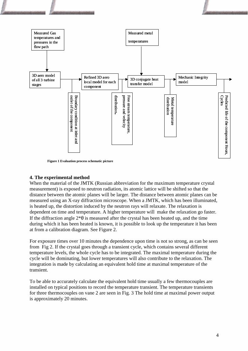
The evaluation process for the measurement is shown in Fig 1. In the following, the results forthe temperature attenuation throughout the turbine stages and the thermal results for blade 2will be presented.

4

3D aero model of all 3 turbine stages

Measured Gas temperatures and pressures in the flow path

Refined 3D aero local model for each component

3D conjugate heat transfer model

Measured metal

temperatures

Mechanic Integrity model

Boundary condition at inlet and outlet of the com

ponent

Free stream tem

perature, pressure

and velocity

distribution.

Metal tem

perature distribution

Predicted life of the component H

ours, C

ycles

3D aero model of all 3 turbine stages

Measured Gas temperatures and pressures in the flow path

Refined 3D aero local model for each component

3D conjugate heat transfer model

Measured metal

temperatures

Mechanic Integrity model

Boundary condition at inlet and outlet of the com

ponent

Free stream tem

perature, pressure

and velocity

distribution.

Metal tem

perature distribution

Predicted life of the component H

ours, C

ycles

Figure 1 Evaluation process schematic picture

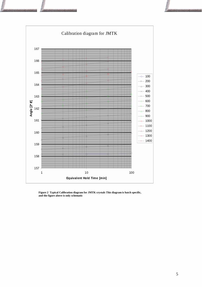
4. The experimental methodWhen the material of the JMTK (Russian abbreviation for the maximum temperature crystalmeasurement) is exposed to neutron radiation, its atomic lattice will be shifted so that thedistance between the atomic planes will be larger. The distance between atomic planes can bemeasured using an X-ray diffraction microscope. When a JMTK, which has been illuminated,is heated up, the distortion induced by the neutron rays will relaxate. The relaxation isdependent on time and temperature. A higher temperature will make the relaxation go faster.If the diffraction angle 2*θ is measured after the crystal has been heated up, and the timeduring which it has been heated is known, it is possible to look up the temperature it has beenat from a calibration diagram. See Figure 2.

For exposure times over 10 minutes the dependence upon time is not so strong, as can be seenfrom Fig 2. If the crystal goes through a transient cycle, which contains several differenttemperature levels, the whole cycle has to be integrated. The maximal temperature during thecycle will be dominating, but lower temperatures will also contribute to the relaxation. Theintegration is made by calculating an equivalent hold time at maximal temperature of thetransient.

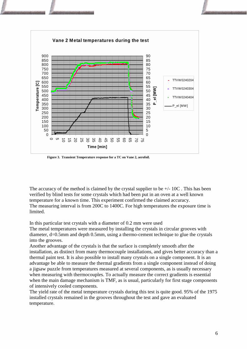
To be able to accurately calculate the equivalent hold time usually a few thermocouples areinstalled on typical positions to record the temperature transient. The temperature transientsfor three thermocouples on vane 2 are seen in Fig. 3 The hold time at maximal power outputis approximately 20 minutes.

5

Evaluation diagram for Thermocrystals of SiC(Here shown for every 100 C only)

157

158

159

160

161

162

163

164

165

166

167

1 10 100

Equivalent Hold Time [min]

Angl

e [2

*]

10020030040050060070080090010001100120013001400

Calibration diagram for JMTK

Figure 2 Typical Calibration diagram for JMTK crystals This diagram is batch specific,and the figure above is only schematic

6

Vane 2 Metal temperatures during the test

050

100150200250300350400450500550600650700750800850900

0 5 10 15 20 25 30 35 40 45 50 55 60 65 70 75

Time [min]

Tem

pera

ture

[C]

051015202530354045505560657075808590

P_el

[MW

]

TTVW0240204

TTVW0240304

TTVW0240404

P_el [MW]

Figure 3. Transient Temperature response for a TC on Vane 2, aerofoil.

The accuracy of the method is claimed by the crystal supplier to be +/- 10C . This has beenverified by blind tests for some crystals which had been put in an oven at a well knowntemperature for a known time. This experiment confirmed the claimed accuracy.The measuring interval is from 200C to 1400C. For high temperatures the exposure time islimited.

In this particular test crystals with a diameter of 0.2 mm were usedThe metal temperatures were measured by installing the crystals in circular grooves withdiameter, d=0.5mm and depth 0.5mm, using a thermo-cement technique to glue the crystalsinto the grooves.Another advantage of the crystals is that the surface is completely smooth after theinstallation, as distinct from many thermocouple installations, and gives better accuracy than athermal paint test. It is also possible to install many crystals on a single component. It is anadvantage be able to measure the thermal gradients from a single component instead of doinga jigsaw puzzle from temperatures measured at several components, as is usually necessarywhen measuring with thermocouples. To actually measure the correct gradients is essentialwhen the main damage mechanism is TMF, as is usual, particularly for first stage componentsof intensively cooled components.The yield rate of the metal temperature crystals during this test is quite good. 95% of the 1975installed crystals remained in the grooves throughout the test and gave an evaluatedtemperature.

7

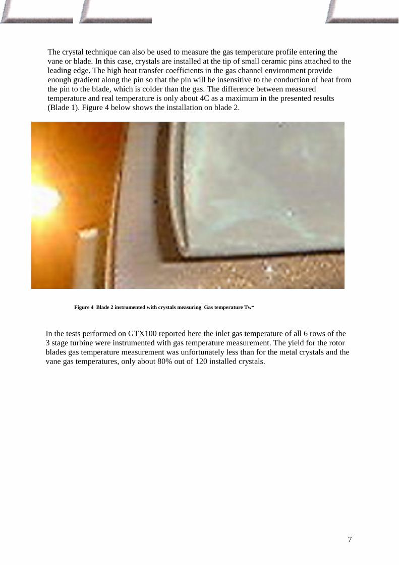
The crystal technique can also be used to measure the gas temperature profile entering thevane or blade. In this case, crystals are installed at the tip of small ceramic pins attached to theleading edge. The high heat transfer coefficients in the gas channel environment provideenough gradient along the pin so that the pin will be insensitive to the conduction of heat fromthe pin to the blade, which is colder than the gas. The difference between measuredtemperature and real temperature is only about 4C as a maximum in the presented results(Blade 1). Figure 4 below shows the installation on blade 2.

7

Figure 4 Blade 2 instrumented with crystals measuring Gas temperature Tw*

In the tests performed on GTX100 reported here the inlet gas temperature of all 6 rows of the3 stage turbine were instrumented with gas temperature measurement. The yield for the rotorblades gas temperature measurement was unfortunately less than for the metal crystals and thevane gas temperatures, only about 80% out of 120 installed crystals.

8

5. Measured gas temperature attenuation vs. gas temperatures from 3D NS multistagecalculations

When designing the cooling system for cooled components in modern gas turbines it isnecessary to spend a minimum of cooling air, in order to minimise the negative effect on theefficiency from the cooling air injection. This means the cooling has to be tailor-made for thegas temperature distributions of the particular turbine.

Most CFD codes have difficulty in correctly predicting the mixing of the flow as it passesthrough the turbine, and thus the temperature attenuation through it. Usually the averagetemperature can be predicted with good accuracy, but it is more difficult to predict the shapeof the temperature profile. In this paper the measurement results are compared to the resultsfrom a 3D NS calculation using the code Stage3D.

This kind of test also provides valuable information for verification of CFD codes.

5.1. 3D Description of the CFD calculations

This chapter give a brief description of the CFD calculations performed in order to haveboundary conditions for the 3D conjugate heat transfer code. A schematic picture of theevaluation process was shown in the introduction, see Fig.1.

An in-house 3D Navier-Stokes solver, MBStage3D, was used to calculate the gas temperatureand other necessary boundary conditions for the conjugate heat transfer calculations. TheCDF calculations were divided into two steps. First a regular simulation of the whole turbinewas performed, then each component was simulated in a separate model, in order to increasethe accuracy by tuning each model against the measured radial temperature distribution.

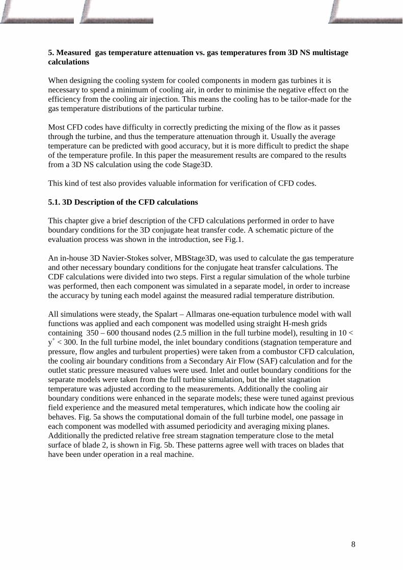
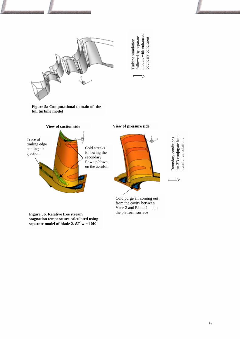
All simulations were steady, the Spalart – Allmaras one-equation turbulence model with wallfunctions was applied and each component was modelled using straight H-mesh gridscontaining 350 – 600 thousand nodes (2.5 million in the full turbine model), resulting in 10 <y+ < 300. In the full turbine model, the inlet boundary conditions (stagnation temperature andpressure, flow angles and turbulent properties) were taken from a combustor CFD calculation,the cooling air boundary conditions from a Secondary Air Flow (SAF) calculation and for theoutlet static pressure measured values were used. Inlet and outlet boundary conditions for theseparate models were taken from the full turbine simulation, but the inlet stagnationtemperature was adjusted according to the measurements. Additionally the cooling airboundary conditions were enhanced in the separate models; these were tuned against previousfield experience and the measured metal temperatures, which indicate how the cooling airbehaves. Fig. 5a shows the computational domain of the full turbine model, one passage ineach component was modelled with assumed periodicity and averaging mixing planes.Additionally the predicted relative free stream stagnation temperature close to the metalsurface of blade 2, is shown in Fig. 5b. These patterns agree well with traces on blades thathave been under operation in a real machine.

9

Turb

ine

sim

ulat

ion

follo

wed

by

sepa

rate

mod

els w

ith e

nhan

ced

boun

dary

con

ditio

ns

Bou

ndar

y co

nditi

ons

for 3

D c

onju

gate

hea

ttra

nsfe

r cal

cula

tions

Figure 5a Computational domain of thefull turbine model

Figure 5b. Relative free streamstagnation temperature calculated usingseparate model of blade 2. ∆∆∆∆T*w = 10K

Cold purge air coming outfrom the cavity betweenVane 2 and Blade 2 up onthe platform surface

Cold streaksfollowing thesecondaryflow up/downon the aerofoil

Trace oftrailing edgecooling airejection

View of pressure sideView of suction side

10

5.2. Measured gas temperature attenuation vs gas temperatures from 3D NS multistagecalculations

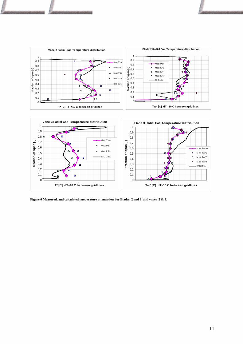
In order to see how well the full turbine simulation predicts the mixing of cooling air to themain stream, the calculated and measured stagnation temperatures were compared. Fig.6shows the results for all the components except the first stage. The measured values areshown by symbols, e.g. 'Mea T*

5' is the measured temperature in the second vane at tangentialposition no. 5 and 'Mea T*

av' is the average of 'Mea T*5', 'Mea T*

22' and 'Mea T*40'. The black

solid lines show the result of the MBStage3D calculations.

The agreement between measurements and calculations is generally fair, the difference is lessthan +/- 20K.

Generally the measured temperatures from the blades are less scattered between differentblades in the same stage than for the vanes. This is logical as the blades scan over the wholeturn, and therefore feel the average temperature. The vanes are stationary and will thus showthe temperature in the particular section where they are positioned, which can differ due totangential temperature variations from the combustor.

Regarding the shape of the calculated stagnation temperatures, the general trends are capturedbut the calculation shows a more oscillating behaviour (the number of measurement pointsshould have been enough to capture this). This indicates that the mixing of the cooling airwith the hot main stream was too slow in the calculations.

In summary, it looks promising for future evaluations of other cases where measurements donot exist. This comparison shows a quite good agreement between calculated and measuredtemperatures.

11

Vane 2 Radial Gas Temperature distribution

0

0,1

0,2

0,3

0,4

0,5

0,6

0,7

0,8

0,9

1

950 1000 1050 1100T* [C] dT=10 C between gridlines

frac

tion

of s

pan

[-]

M ea: T*av

M ea: T*5

M ea: T*22

M ea: T*40

S3D Calc.

Blade 2 Radial Gas Temperature distribution

0

0,1

0,2

0,3

0,4

0,5

0,6

0,7

0,8

0,9

1

820 830 840 850 860 870 880 890 900 910 920Tw* [C] dT= 10 C between gridlines

frac

tion

of s

pan

[-]

M ea: T*av

M ea: Tw*1

M ea: Tw*4

M ea: Tw*7

S3D calc.

Vane 3 Radial Gas Temperature distribution

0

0,1

0,2

0,3

0,4

0,5

0,6

0,7

0,8

0,9

1

750 800 850T* [C] dT=10 C between gridlines

frac

tion

of s

pan

[-] M ea: T*av

M ea:T*13

M ea:T*23

S3D Calc.

Blade 3 Radial Gas Temperature distribution

0

0,1

0,2

0,3

0,4

0,5

0,6

0,7

0,8

0,9

1

600 650 700Tw* [C] dT=10 C between gridlines

frac

tion

of s

pan

[-]

M ea: Tw*av

M ea: Tw*1

M ea: Tw*2

M ea: Tw*3

S3D Calc.

Figure 6 Measured, and calculated temperature attenuation for Blades 2 and 3 and vanes 2 & 3.

12

6. Measured metal temperature distribution of a cooled component, compared toconjugate heat transfer calculations.

The metal temperatures of the components in the gas path are calculated using a 3D metalmodel to which boundary conditions in terms of heat transfer coefficients and fluidtemperatures are coupled. Temperatures on the gas side are taken from the 3D NS calculationsdescribed above, and the heat transfer coefficients are calculated using boundary layerprogrammes. The cooling system inside the blade is described using a 1D flow network. Eachbranch has correlations for heat transfer and pressure losses coupled to it. The calculatedtemperatures are then transferred to the mechanical integrity model used for prediction of thelifetime of the component. One of the main factors which determines the accuracy of thelifetime prediction is how accurately the temperature distribution was predicted.

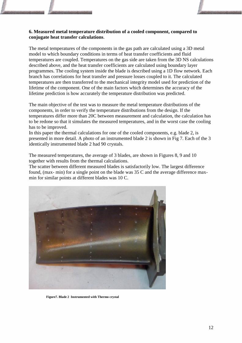
The main objective of the test was to measure the metal temperature distributions of thecomponents, in order to verify the temperature distributions from the design. If thetemperatures differ more than 20C between measurement and calculation, the calculation hasto be redone so that it simulates the measured temperatures, and in the worst case the coolinghas to be improved.In this paper the thermal calculations for one of the cooled components, e.g. blade 2, ispresented in more detail. A photo of an instrumented blade 2 is shown in Fig 7. Each of the 3identically instrumented blade 2 had 90 crystals.

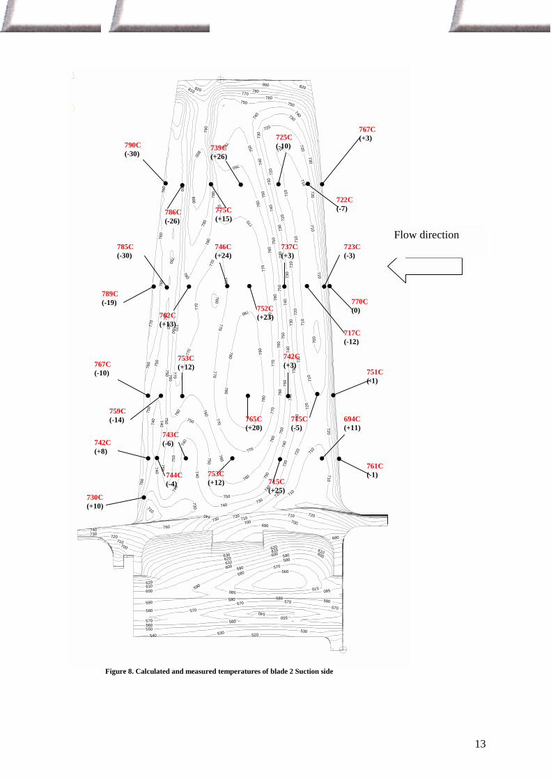
The measured temperatures, the average of 3 blades, are shown in Figures 8, 9 and 10together with results from the thermal calculations.The scatter between different measured blades is satisfactorily low. The largest differencefound, (max- min) for a single point on the blade was 35 C and the average difference max-min for similar points at different blades was 10 C.

Figure7. Blade 2 Instrumented with Thermo crystal

13

520530 530540

540

550

550

560560

560

570

570570 570

570

570

570

580

580 580 580

580580

580

580

590

590

590

590

600

600

600 600

610

610

610 610

620

620

620

630

680

690

700

700 700

700

710

710710

710

710

710

710

710

710

710

710

710

710710

710

720

720

720

720

720

720

720

720

720

720

720

720

720

720

720

730

730

730

730

730

730

730

730

730

730

730

730

730

730

740

740

740 740

740

740

740

740

740

740

740

740

740

740

740

740

740

740

740

750

750

7 50

750750

7 50750

7 50

750

750

750

750

750

750

750

750

750

750

750

750

750 750

750

760

7607 60

760 760

760

760

760

760

760

760

760

760

760

760

760

760

760

760

760

760

760

770770

770

770

770

770770

770770

770

770

770

770

770

770

770

770

770

780

780

780

780

780

780

780

780

780

790

790

800

800800

810820820

730C(+10)

761C(-1)

742C(+8)

743C(-6)

753C(+12) 715C

(+25)

694C(+11)

751C(-1)

767C(-10)

759C(-14)

753C(+12)

765C(+20)

742C(+3)

715C(-5)

723C(-3)

789C(-19)

785C(-30)

762C(+13)

746C(+24)

752C(+23)

737C(+3)

770C(0)

717C(-12)

722C(-7)

790C(-30)

786C(-26)

775C(+15)

739C(+26)

725C(-10)

767C(+3)

744C(-4)

Figure 8. Calculated and measured temperatures of blade 2 Suction side

Flow direction

14

520530 530 540

540

550 550

550

550

560

560

560

560 560 560

560

570 570570

570

570

580

580580

580 580580

580

590

590

590590

600

600

610

610

620

620

630

640

650

660 680

680

690

690

690

690690

690

690

690

690

690

6 90

690690

700

700700

700

700

700

700

700

700

700

700

700700

700

700

700

710

710

710

710

710710

710710

710

710

710

710

710

7 10

710

710

720

720720

720

720 720720

720

720720

720720

720

720

720

720

730

730

730730

730

730

730

730730

730

730730

730

730 730

730

740

740

740

7407 40

740

740

740740

740

740

740

750

750

750

750750

7 50

750

750750 750

750

750

750

750

750

750

760

760760

760760

760

760

760

760

760

760

760

760

760

760

760

760

760760

760760

760760

760

760760

770770

7 70

770770

770770

770

770

7 70

770

770

770

7 70

770

770

7 70

770

780

780

780

780

780

780

790

790

790

790

840

743C(+2)

752C(+13)

749C(-4)

796C(-26) 748C

(-23)761C(-16)

776C(-26)

765C(0)797C

(-17)

748C(-18)

788C(-18)

800C(-30)

785C(-25)

774C(-4)

757C(-2)

776C(-6)

725C(-14)

744C(0)

800C(-35)

799C(-39)

789C(-19)

787C(-12)

713C(-3)

722C(+3)

791C(-31)

771C(+4)

719C(+6)

746C(+34)

767C(+23)

822C(+3)

806C(-1)

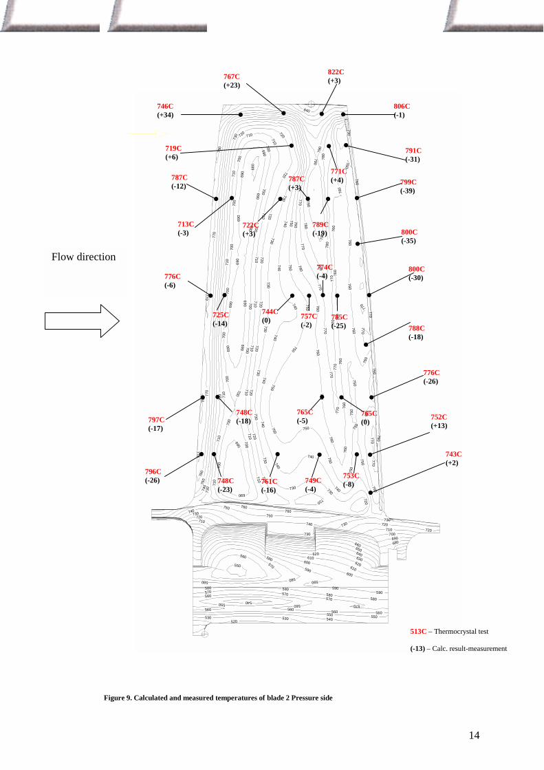
513C – Thermocrystal test

(-13) – Calc. result-measurement

753C(-8)

765C(-5)

787C(+3)

Figure 9. Calculated and measured temperatures of blade 2 Pressure side

Flow direction

15

675

680

680

685

690

690

690

695700

705

705710

710710

715

715

715

715

720

720

720

720

720

720

725

725

725

725

725

725

730

730

730

730730

730

730730

735

735

735

735735

735

735

735735735

740

740740

740740

740

740

74074074074

074

0

740

745

745

745745

745

745745 74

5

750

750

750750

750

750

750

750

755

755

755

755

755

760

760

760

760

760

765

765

765

765

770

770

770

770

775

775

780

785795

805810

820

825

830

731C(+9)

657C(+36)

740C(+5)

744C(+3)

721C(-6)

758C(+2)

751C(+1)

733C(+14)

729C(+4)

513C – Thermocrystal test

(-13) – Calc. result-measurement

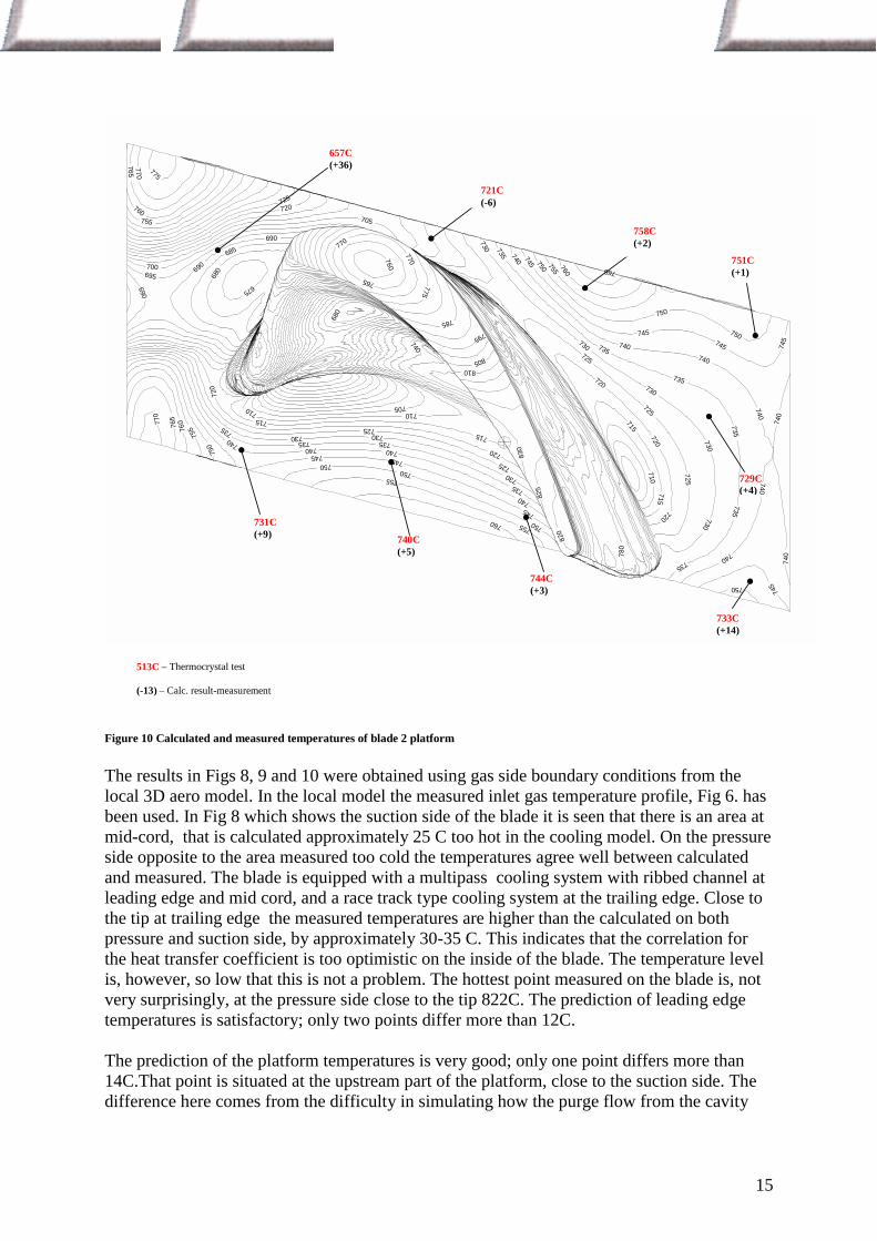
Figure 10 Calculated and measured temperatures of blade 2 platform

The results in Figs 8, 9 and 10 were obtained using gas side boundary conditions from thelocal 3D aero model. In the local model the measured inlet gas temperature profile, Fig 6. hasbeen used. In Fig 8 which shows the suction side of the blade it is seen that there is an area atmid-cord, that is calculated approximately 25 C too hot in the cooling model. On the pressureside opposite to the area measured too cold the temperatures agree well between calculatedand measured. The blade is equipped with a multipass cooling system with ribbed channel atleading edge and mid cord, and a race track type cooling system at the trailing edge. Close tothe tip at trailing edge the measured temperatures are higher than the calculated on bothpressure and suction side, by approximately 30-35 C. This indicates that the correlation forthe heat transfer coefficient is too optimistic on the inside of the blade. The temperature levelis, however, so low that this is not a problem. The hottest point measured on the blade is, notvery surprisingly, at the pressure side close to the tip 822C. The prediction of leading edgetemperatures is satisfactory; only two points differ more than 12C.

The prediction of the platform temperatures is very good; only one point differs more than14C.That point is situated at the upstream part of the platform, close to the suction side. Thedifference here comes from the difficulty in simulating how the purge flow from the cavity

16

before the blade is distributed. The distribution is dependent on unsteady effects and localgeometry features that are not resolved in the degree of detail of the used3D aero model.The measurement confirms the metal temperature level of blade 2 from the design project ofthe engine.

7. ConclusionAfter the successful performance of the test it must be stated that using thermo-crystals is areliable test method. It provides the possibility to measure temperatures in detail and pick upthe temperature gradients with good accuracy, particularly for rotating blades.There is generally good correlation between measurements and calculations, which givesconfidence in the used calculation methods, and correlations. However, to ascertain a betterprediction of the gas temperature distributions in future the proposal is to use unsteady CFDanalysis as standard.

During the test several areas with potential for saving cooling air have been identified.

8. References

1. V.A Nikolaenko, V. I. Karnushin. Year 1986. Measurement of temperatures usingirradiated materials.2. V.A Nikolaenko,V.A Morosov,N.I. Kasianov. Rev. int. Temp et Refract 1976 t.13 pp 17-20