Embed Size (px)
Citation preview

Guidance for tailoring material to its life cycle environment profile mechanical environment
08/02/2010
Edition 0 DRAFT UNCLASSIFIED
Guide for tailoring material to its life cycle environment profile. Mechanical environment Page 1/282
GUIDANCE FOR TAILORING MATERIAL TO ITS LIFE CYCLE
ENVIRONMENT PROFILE. MECHANICAL ENVIRONMENT

Guidance for tailoring material to its life cycle environment profile mechanical environment
08/02/2010
Edition 0 DRAFT UNCLASSIFIED
Guide for tailoring material to its life cycle environment profile. Mechanical environment Page 2/282
SUMMARY
OBJECT OF THE DOCUMENT .............................................................................. 8
1. INTRODUCTION .............................................................................................. 9
1.1. Preamble ............................................................................................................................ 9
1.2. Stakes ............................................................................................................................... 10
1.3. Tailoring process for the mechanical environment ..................................................... 10 1.3.1. Use of the tailoring process ........................................................................................... 10 1.3.2. Step 1 - Establishment of system life cycle environment profile .................................. 12 1.3.3. Step 2 - Determination of the real environmental data associated with each situation . 12 1.3.4. Step 3 - Determination of the withhold environment to be simulated ........................... 12 1.3.5. Stage 4 - Establishment of the qualification or design approval program (demonstration by calculation, test or simulation) ............................................................................................... 13
1.4. Responsibilities in the application for tailoring process .............................................. 13
1.5. Initial and tailored tests severities ................................................................................. 14
2. PRINCIPAL METHODS OF THE TAILORING PROCESS FOR MECHANICAL ENVIRONMENT ......................................................................... 17
2.1. Methods by envelope of PSD .......................................................................................... 17
2.2. Advantages and disadvantages of the method by envelope of PSD ............................ 21
2.3. Method by equivalence of Damage ................................................................................ 21
2.4. Advantages of the method by equivalence of fatigue damage .................................... 22
2.5. Comparison of the assumptions between the method of envelope of the PSD and the method of equivalence of fatigue damage .................................................................................. 23
3. STEP 1 - LIFE PROFILE ................................................................................ 24
3.1. Contents and exploitation of an environment life profile ........................................... 24
3.2. More detailed examples of establishment of an environment life profile. ................. 26
4. STEP 2 - CHARACTERIZATION OF THE REAL ENVIRONMENT ..... 27
4.1. Characterization of the environmental agents ............................................................ 27 4.1.1. Characterization by nature ............................................................................................. 27 4.1.2. Characterization by signal class of a mechanical environment agent ........................... 27 4.1.3. Characterization as a function the data origin ............................................................... 28 4.1.4. Characterization according to the level of assembly and the activated function .......... 28
4.2. Definition of the physical parameters ........................................................................... 29
4.3. Criteria and tools allowing measurement validation ................................................... 29

Guidance for tailoring material to its life cycle environment profile mechanical environment
08/02/2010
Edition 0 DRAFT UNCLASSIFIED
Guide for tailoring material to its life cycle environment profile. Mechanical environment Page 3/282
5. STEP 3 - DETERMINATION OF THE ENVIRONMENT TO BE SIMULATED ............................................................................................................. 30
5.1. Principles and laws of equivalences in terms of extreme response spectra and fatigue damage spectra ............................................................................................................................. 30
5.2. Assumptions retained for the behavior of materials ................................................... 31
5.3. Choice of the rheological model of material behavior ................................................. 31
5.4. Definition of SRS, ERS, XRS and FDS spectra ............................................................ 32 5.4.1. Shock Response Spectrum (SRS) .................................................................................. 32 5.4.2. Extreme Response Spectrum (ERS) .............................................................................. 33 5.4.3. Up-crossing risk spectrum (URS) .................................................................................. 33 5.4.4. Fatigue Damage Spectrum (FDS) .................................................................................. 37 5.4.5. Choice of the most suitable calculation method: PSD or temporal signal .................... 39
5.5. Consideration of the environment data variability...................................................... 40
5.6. Consideration of the mechanical characteristics variability ....................................... 41 5.6.1. Failure by extreme stress ............................................................................................... 42 5.6.2. Fatigue failure ................................................................................................................ 42
5.7. The coefficient of guarantee: formulation and calculation principle ......................... 42 5.7.1. Interaction between two normal distributions ............................................................... 44 5.7.2. Interaction between two log-normal distributions ......................................................... 46 5.7.3. Interaction between two Weibull distributions .............................................................. 47
5.8. Synthesis of all life profile situations ............................................................................. 49 5.8.1. Treatment of each event ................................................................................................ 49 5.8.2. Criteria of regrouping of the events of a situation or synthesis of several situations .... 50 5.8.3. Synthesis of the events of a situation ............................................................................. 50 5.8.4. Synthesis of several situations ....................................................................................... 53
5.9. Particular case: taking into account of an environment of the “repeated shocks” type 54
5.9.1. By reducing the number of shocks and by increasing their amplitude to respect the fatigue damage ............................................................................................................................ 54 5.9.2. By determining the characteristics of a random vibration of the same severity............ 55
6. STAGE 4 - DRAFTING OF THE TEST PROGRAMME ........................... 59
6.1. Severities of the tests appearing in the normative documents .................................... 59
6.2. Contents of a test programme ........................................................................................ 61 6.2.1. List of applicable methods ............................................................................................. 61 6.2.2. Choice of the test procedures ......................................................................................... 61 6.2.3. Determination of test severities ..................................................................................... 61 6.2.4. Tests chronology ............................................................................................................ 61 6.2.5. Amount of specimen under tests.................................................................................... 62 6.2.6. Sanctions ........................................................................................................................ 62
6.3. Need and calculation of the test factor .......................................................................... 63 6.3.1. Necessity of the test factor ............................................................................................. 63

Guidance for tailoring material to its life cycle environment profile mechanical environment
08/02/2010
Edition 0 DRAFT UNCLASSIFIED
Guide for tailoring material to its life cycle environment profile. Mechanical environment Page 4/282
6.3.2. Test factor calculation for the normal distribution: ....................................................... 63 6.3.3. Test factor calculation for the log-normal distribution .................................................. 64 6.3.4. Test factor calculation for the Weibull distribution: ..................................................... 65
6.4. Reduction of the test duration ....................................................................................... 66
6.5. Validation of the time reduction .................................................................................... 67
6.6. Return to PSD starting from the FDS ........................................................................... 71
6.7. Return to PSD starting from the ERS ........................................................................... 71
6.8. Notice on the specification of the shocks by a SRS ...................................................... 71
6.9. Possibility of splitting a band in several (generally 2) sub-bands .............................. 71
6.10. Test Rigs ........................................................................................................................... 72 6.10.1. Frame of loading/testing machine .............................................................................. 72 6.10.2. Tables of generator of vibrations ............................................................................... 72 6.10.3. Specific loading but through a flexible coupling ....................................................... 73 6.10.4. Mono excitation axial and multi point ....................................................................... 73 6.10.5. Excitation multiaxial and Mono point ........................................................................ 73 6.10.6. Excitation multiaxial and multi point ......................................................................... 73
6.11. Relative questions with the triaxial aspect of the real environment .......................... 73 6.11.1. Triaxial excitation mono point ................................................................................... 74 6.11.2. Mono axial or triaxial excitation multipoint: ............................................................. 75
6.12. Mechanical environments low frequency - static field - quasi-static ......................... 75 6.12.1. Position of the problem .............................................................................................. 75 6.12.2. Examples of the missiles integrated under plane subjected to the shocks of landing 77
6.13. Representativeness and reproducibility of the tests .................................................... 78
7. RECOMMENDATIONS ON THE CHOICE OF THE VALUES OF THE PARAMETERS ......................................................................................................... 80
7.1. Choice of the value b ....................................................................................................... 80 7.1.1. Usual values ................................................................................................................... 80 7.1.2. Recommended value ...................................................................................................... 81
7.2. Choice of the damping of the system standard ............................................................ 82
7.3. Choice of the values K and C ......................................................................................... 83
7.4. Calculation of the MRS .................................................................................................. 83
8. ANNEXES ......................................................................................................... 92
8.1. Representation of the Wöhler curve ............................................................................. 92 8.1.1. WÖHLER Curve : fatigue tests with imposed constraint .............................................. 93 8.1.2. Analytical modeling of the WÖHLER curve ................................................................ 94
8.2. guarantee Coefficient and test factor : abacuses .......................................................... 96
8.3. Calculation of the MRS ................................................................................................ 118
8.4. Historical background .................................................................................................. 128

Guidance for tailoring material to its life cycle environment profile mechanical environment
08/02/2010
Edition 0 DRAFT UNCLASSIFIED
Guide for tailoring material to its life cycle environment profile. Mechanical environment Page 5/282
8.5. Measurements validation ............................................................................................. 128 8.5.1. general Criteria ............................................................................................................ 129 8.5.2. specific Criteria ............................................................................................................ 130
8.6. Synthesis of the environment without taking into account the FDS ....................... 131 8.6.1. Illustration on a nonstationary signal of the disadvantages of the PSD envelope method : 131 8.6.2. Case of a carrying under plane .................................................................................... 134 8.6.1. Logistic cases of transport or transport or tactical carryings ....................................... 139
8.7. Determination of the data which characterize the agents of environment : their origin and the level of assembly to which they are referred ................................................... 139
8.8. Taking into account of the limitations of the test facilities ....................................... 147 8.8.1. Dependent limitations has the complexity of the real vibratory environment ............ 147 8.8.2. Limitations related to the performances of the means of generation of the vibrations and the shocks ........................................................................................................................... 147 8.8.3. Limitations related to the average means of ................................................................ 147 8.8.4. Limitations resulting from the difficulty of recreating the dynamic interaction between material and its carrier .............................................................................................................. 148 8.8.5. Limitations due has the difficulty in recreate the true initial conditions ..................... 148 8.8.6. Other Limitations ......................................................................................................... 148
8.9. Complements on the organization of the test routine ................................................ 149 8.9.1. Work relating to the process of test ............................................................................. 149 8.9.2. Realization of the testing apparatus ............................................................................. 153 8.9.3. Validation of the design of the test ............................................................................. 154 8.9.4. Costs and times ........................................................................................................... 154 8.9.5. Realization of the test ................................................................................................. 154 8.9.6. Review contract of execution ............................................... Erreur ! Signet non défini.
8.10. Reduction of duration of test – Example .................................................................... 155
8.11. Assistance with the choice of the sanctions ................................................................ 159 8.11.1. Code of sanction ...................................................................................................... 161 8.11.2. Resulted in holding in the event of incidents during the tests .................................. 162
8.12. To neglect or not the static component ....................................................................... 163
9. EXAMPLE ON PROFILE OF LIFE SIMPLIFIES ....... ERREUR ! SIGNET NON DEFINI.
9.1. Input data ...................................................................................................................... 164
9.2. Characterization of the Logistic Situation of Transport per Road Way S1 ............ 166 9.2.1. Case of the S1.1 event: Handling Shock .................................................................... 166 9.2.2. Case of the S1.2 event: rough road Vibrations ............................................................ 168 9.2.3. Case of the event S1.3: Vibrations Good Road .................. Erreur ! Signet non défini. 9.2.4. Synthesis of the events S1.1, S1.2 and S1.3 ................................................................ 182
9.3. Characterization of the Logistic Situation of Transport per Road S2 .................... 187
9.4. Characterization of the Logistic Situation of Transport by air S3 .......................... 189
9.5. Characterization of the Logistic Situation of Transport per S4 Railway ................ 194

Guidance for tailoring material to its life cycle environment profile mechanical environment
08/02/2010
Edition 0 DRAFT UNCLASSIFIED
Guide for tailoring material to its life cycle environment profile. Mechanical environment Page 6/282
9.6. Characterization of the Tactical Situation of Transport on Any S5 Way ............... 197
9.7. Characterization of the Tactical Situation of Transport on Any S6 Ground ......... 199
9.8. Synthesis of the two Situations of Tactical Transport S5 and S6 ............................. 202
9.9. Synthèse des quatre Situations de Transport Logistique S1, S2, S3 et S4 ............... 204 9.9.1. Synthesis of the two Situations of Logistic Transport S3 and S4 ............................... 205 9.9.2. Synthesis of the three Situations of Logistic Transport S1, S2 and S3/S4 .................. 209
9.10. Specifications of tests associated with the self-propelled gun subjected to the simplified life profile .................................................................................................................. 212
9.10.1. Specification of tests associated with the Situations with Tactical Transport S5 and S6 212 9.10.2. Specification of tests associated with the Logistic Situations of Transport S1 with S4 218
10. EXAMPLE 2: LIFE PROFILE OF A WEAPON SYSTEM ...................... 227
10.1. Step 1: List of the situations ........................................................................................ 227
10.2. Stage 2: Determination of the environment associated with the situations ............. 231
10.3. Stage 3: Synthesis of the situations .............................................................................. 234 10.3.1. Parameters for the synthesis ..................................................................................... 234 10.3.2. Analyzes of random vibrations ............................................................................... 234 10.3.3. Analyzes shocks ....................................................................................................... 245
10.4. Step 4: Establishment of the qualification program .................................................. 248 10.4.1. Test routine for the random vibration ...................................................................... 248 10.4.2. Test programme for the shocks ............................................................................... 253 10.4.3. Comparison test specification in PSD VS. initial PSD spectrum. ........................... 261
11. EXAMPLE 3: DEVELOPMENT OF A LIFE PROFILE FOR A CIVIL APPLICATION EQUIPMENT ........................................................................... 265
REFERENCES ........................................................................................................ 273

Guidance for tailoring material to its life cycle environment profile mechanical environment
08/02/2010
Edition 0 DRAFT UNCLASSIFIED
Guide for tailoring material to its life cycle environment profile. Mechanical environment Page 7/282
GLOSSARY OF THE ACRONYMS AND SYMBOLS LIST
CG Guarantee Coefficient CVr Variation of stress Coefficient CVe Variation of environment Coefficient CoG Centre of Gravity DOF Degree Of Freedom ERS Extreme Response Spectrum FEA Finite Element Analysis FE Test Factor PSD Power Density Spectrum URS Up-crossing Risk Spectrum FDS Fatigue Damage Spectrum UFS Up-crossung risk Fatigue Spectrum SRS Shock Response Spectrum

Guidance for tailoring material to its life cycle environment profile mechanical environment
08/02/2010
Edition 0 DRAFT UNCLASSIFIED
Guide for tailoring material to its life cycle environment profile. Mechanical environment Page 8/282
OBJECT OF THE DOCUMENT
The object of this document is to constitute a guide for Tailoring a material to its Life Cycle Environmental Profile, for the mechanical environment. It is a response to the actual orientations of Defence that are to reduce the materials development costs, their deployment and maintenance in the defense services.
It addresses to: directors and program officers , test program specificators, research departments, calculation offices,… official and industrialists who will find a referential
in matter of managing the mechanical environment by tailoring of the material to its life cycle profile.
The mechanical environment considered in this guide is not limited in theory to the vibrations, the
shocks, the constant acceleration or the acoustic vibration usually simulated by generators of vibrations, shock machines, centrifugal machines or acoustic reverberating rooms. However in fact, all occurs as if it were the case because the standardized testing methods to which one refers for the establishment of the test programme are those which call upon these test facilities.
The reality of the mechanical environment requests a very varied nature: aerodynamic fluctuations distributed or local and of which the effects are difficult to simulate differently out of an air blower, mechanical fatigue of devices intervening in rough operational material deployments and whose effects are not represented by tests on shakers or on shock machine.
It is necessary to admit that although the mechanical term of environment is general, this guide does not cover, except for the chapter on the life profile system, only the part of the mechanical environments which calls upon the most current test facilities knowing mainly the shakers, the shock machines, the centrifugal machines and the reverberating acoustic rooms.
The mechanical environment in this guide relates to the vibrations, the shocks and static or quasi
static accelerations and the acoustic vibrations whose taking into account is relevant within the framework of the qualification/or design approval tests These tests are contractual and are intended to prove by the prime contractor or its sub contractors of the good behavior of the material in presence of the expected life cycle profile environment.
They should not lead to restart a structural sizing at high level of assembly, as it could be the case for the static and fatigue tests at the beginning of the development. The failures to which the tests in mechanical environment lead are not easily predictable and as moreover they are not generally dimensioning (sizing) ; that explains why it did not have traditionally strong links between the calculation office and the environmental test lab , contrary to the case of the static tests and structural low frequency (“low cycle” ) fatigue test lab .
For the special environments not covered in the collections of standardized testing methods, the prime contractor can always engage a specific test which it will remain a design validation test ( with the aim to validate the technical functions ) or will become a qualification test or design approval ( with the aim to validate the service functions). The reproducibility of the not standardized method implemented if necessary must be validated by the prime contractor.

Guidance for tailoring material to its life cycle environment profile mechanical environment
08/02/2010
Edition 0 DRAFT UNCLASSIFIED
Guide for tailoring material to its life cycle environment profile. Mechanical environment Page 9/282
1. INTRODUCTION
1.1. Preamble
The method of writing the tests specifications, as presented in the standards, GAM-EG-13 [GAM 86], DEF STAN 0035 (GB) [DEF **], MIL STD 810 (US) [MIL **], or standards NATO STANAG 4370 [OTA **] which followed, related to the tailoring of the “environmental tests”, defined according to the life profile of the material.
The use of the GAM-EG-13 is only valid for the materials in service and not for the programs in the
acquisition process and futures for which the STANAG 4370 and the interallied publications covered by this STANAG are recommended by the French RNPA ( Référentiel Normatif Pour l’Armement / French Ministry of Defense)..
An “environmental test” comprises the application of forcing functions ( the environmental agents
applied to the material) and associated functional measurements . It is useful to recall that historically the “environmental tests” were defined many years ago via the admission tests . Later the concept of “Qualification” at the end of the development appeared. In practice, majority of tests, even tailored, intervened subsequently to definition choices, which resulted in too tardily analysing problems which should have been solved before, with important consequences on the costs and delays.
The taking into account of the first results of “in situ measurements ” in addition made inevitable
the execution of certain “tailored” tests, not envisaged initially in the Programme, from where systematic increase of budgets and non respected deadlines. The best manner of avoiding these errors is to take into account the factors related to the environment at the beginning of the material development.
This justified an evolution aiming at supplementing the initial concept of “tailoring tests” by various
actions implemented during the life cycle of the product, since the beginning of the development until the withdrawal of the service: this method corresponds to the concept of Tailoring a material to its Life Cycle Profile Environment (LCEP) .
The method has been developed in a French document: CIN EG1 [CIN **] which guides the
various official and industrial actors for tailoring a material to its Life Cycle Profile Environment in order to reduce the costs ( development and deployment ). CIN EG 1 does not have really an equivalent on the international plan ; it is in the course of revision and of integration in collection NORMDEF (France) .
The deliberate choice was made, in this guide, to privilege the technical bases and concepts rather
than the organisational steps. As a good part of these technical bases found in the method of tailoring of the tests, it is this approach which structured in fact this document.
The taking into account of the mechanical environment during the material life profile , object of
this guide, is based on the concept of tailoring. When one is confronted with a lack of data at the beginning of a project, it is however allowed to refer to initial severities. However, it will be necessary as soon as possible to replace these initial values by tailored ones.

Guidance for tailoring material to its life cycle environment profile mechanical environment
08/02/2010
Edition 0 DRAFT UNCLASSIFIED
Guide for tailoring material to its life cycle environment profile. Mechanical environment Page 10/282
1.2. Stakes
The field covered by the general environmental standards concerns the constraints of mechanical environment (forced, vibrations, shocks…), climatic (temperatures, humidity…) and electromagnetic (electromagnetic aggressions and compatibility). The object of these standards is to organize the client - supplier relationship in order to optimize the taking into account of the environments in the design and manufacture of the materials. This comprises technical sides (how to make), as well as shared responsibilities (who do what).
The principal idea of the general environmental standards in the sector of defense is to allow, when it is useful, the implementation of the tailoring method. In opposition to the civil standards (like the IEC), which seeks in particular the standardization of preferential severities, it is a question of adapting the specifications of a system so as to satisfy “just” the performances sought, which is economically justified for systems carried out in very small series, such as the defence systems.
With this principal idea the will of the prime contractor is to reach the required operational
performances for the whole of the deployment field, rather than on a limited field by a number of agreed tests.
It is thus the prime contractor which defines the test programme at all the levels of assembly and is
committed on the capacity of this test programme to demonstrate the good behaviour of the system on the whole field of application. The role of the procurement authority is to specify and translate, in technical terms, the field of application indicated in the expression of need “upstream”. For example, when this expression indicates that a fighter plan must resist the shock of landing, it is the procurement authority which specifies this aggression at the entry system.
Within this framework of responsibilities, environmental test standards : frame the technical and tailored specification need for the procurement authority, guide the contractors in the tailoring process in a way adapted on need, like in the development of
tests severities , define the test methods which the contractors must use.
Thus, the environmental standards are specific for Defence and structure the division of the
contractual liabilities associated with this aspect for the programs for armament.
1.3. Tailoring process for the mechanical environment
1.3.1. Use of the tailoring process
An environment can belong to three domains, definite by the effective performance of the function of a material compared to the expected performance. There are not a domain of environment which would be “normal”, a domain which would be “limit” and a domain which would be “extreme”. These domains are defined compared to the expected functional level performances and thus change from one performance with another of the same function or from a function to another.

Guidance for tailoring material to its life cycle environment profile mechanical environment
08/02/2010
Edition 0 DRAFT UNCLASSIFIED
Guide for tailoring material to its life cycle environment profile. Mechanical environment Page 11/282
A given environment can, according to the material and the function considered, the expected performance of the function, to belong to various domains :
the normal domain, for which the function considered of the material must be assured with the specified performance levels,
the limit domain, for which the function considered of the material can present a degraded performance, while respecting the safety requirements; this degradation having to be reversible when one returns in the normal domain,
the extreme domain, for which the function considered of the material can present an irreversible performance degraded while respecting the safety requirements.
In France, the Technical Specification part dedicated to environmental aspects (Steps 1 and 2 of the
tailoring process such as below definite) emitted by French Ministry of Defense , is limited to the normal domain at system level. The other domains are treated elsewhere in the TS system.
The tailoring process comprises four steps: the step 1 number one consists in counting the situations met during the life of the material, the step 2 consists in determining real data of environment associated with the agents of
environment associated to each situation, the step 3 consists in determining the environment known as selected in order to be simulated, the step 4 consists in establishing the test programme.
The following types of environment are distinguished:
real environment: o awaited environment : it is the environment which one describes in a request for
proposals, o specified environment: it is the environment which one describes in the TS of the various
levels of the system tree structure , environment withhold : it is a point of required passage before determining test severities (which
this test is real or which one utilise this severity in a model of validation): it is obtained by multiplying the average environment derived by application of the guarantee coefficient , which takes into account the variabilities of the environment and of the resistance to this environment. It would be the severity of the test if the material under test had a resistance variability to the environment considered null. In fact, it is never the case,
the test severity : it is the transformation of the withhold environment which takes into account the material variability of resistance ; it is obtained by multiplying the withhold environment by the test factor .

Guidance for tailoring material to its life cycle environment profile mechanical environment
08/02/2010
Edition 0 DRAFT UNCLASSIFIED
Guide for tailoring material to its life cycle environment profile. Mechanical environment Page 12/282
1.3.2. Step 1 - Establishment of system life cycle environment profile
This first step consists in analyzing the material use from its exit of factory until its service withdrawal (by destruction or dismantling) in order to make a chronological description of the situations met (including the maintnance and the missions).
Each situation is defined by: its type: handling, logistic transport, storage, tactical carrying,…, its duration, its occurrence, its geographical place, of the corresponding specific data:
o transport logistic: carrier, paces, position of the material during transport,… o storage: under shelter with weak or great thermal inertia, with open sky, with or without
stacking,… o various agents of environment present during the situation: agents climatic, mechanical,
electromagnetic,…
The establishment of the life cycle environment profile is deduced from the system life profile ; it consists to identify and retain the condition of uses likely to generate “significant” mechanical environments which the material will see during its life.
1.3.3. Step 2 - Determination of the real environmental data associated with each situation
The environmental data associated with each situation must be closest to the real conditions. Several cases can be met: the real environment is accessible: the measurements raised under conditions identical or close to
those of the situation considered are available or can be realized, the real environment can be estimated: the environment can be estimated starting from real data
and modelling, the real environment is unknown: in this case, initial severities are used. They are consisted values
corresponding to situations similar (with carriers or shelters identical) or data appearing in various r.
1.3.4. Step 3 - Determination of the withhold environment to be simulated
The withhold environment is deduced from the whole of the environments determined at step 2. The environments corresponding to certain situations that could be gathered if these situations would disclose similar states, configurations and characteristics of environment. For a given agent, some situations could be neglected since they have too low constraints to involve a significant damage of the material.

Guidance for tailoring material to its life cycle environment profile mechanical environment
08/02/2010
Edition 0 DRAFT UNCLASSIFIED
Guide for tailoring material to its life cycle environment profile. Mechanical environment Page 13/282
1.3.5. Stage 4 - Establishment of the qualification or design approval program (demonstration by calculation, test or simulation)
The qualification program (demonstration by calculation, test, or simulation) will be established
starting from the withhold environment, determined at step 3 and by taking account of the following elements:
existence of procedures of tests defining the methods to be applied, existence of the test facilities with relevant performances, state and configuration of the material, chronology of the tests (which must be coherent with that of the life profile), feasibility and cost of the tests, etc
1.4. Responsibilities in the application for tailoring process The responsibilities in the application for tailoring process are described in table 1.1.
Objective within the framework of the program
Formalization Responsibility
Concept of employment: system Life Cycle Profile
Environmental Specifications at system
level
Stage 1 List of the situations met during the life of the material
Procurement authority
Stage 2 Determination of the real data of environment associated with each situation
Procurement authority
Life cycle environment profile
Stage 1 Extraction starting from the system life profile corresponding to the significant mechanical environments
Prime Contractor
Design: industrial application
Stage 3 Determination of the withhold environment
Prime Contractor (and subcontractors)
Program qualification Stage4 Establishment of the qualification program (demonstration by calculation, test or simulation)
Prime Contractor (and subcontractors)
Table1-1: Responsibility in the application for the tailoring process

Guidance for tailoring material to its life cycle environment profile mechanical environment
08/02/2010
Edition 0 DRAFT UNCLASSIFIED
Guide for tailoring material to its life cycle environment profile. Mechanical environment Page 14/282
1.5. Initial and tailored tests severities
Initial tests severities are those resulting from the standards, the normative repertories, recommendations based on the “ in house” experience feedback attached for a type of equipment. One finds there, according to the type of equipment and the use and installation requirements of this one, the indications on test severities to be applied. Initial severities can be sometimes elaborate on the basis of a standard profile of life.
But whole or part of the tailoring process must be engaged since: the differences between the possible life profile having been used for the development of initial
severity and the real life profile are significant, or that the data taken into account for its development are not representative, or that the conditions of its obtaining are not explicit.
In certain cases, one uses the term of “refuge”severity , whose character even of refuge is explicit
(the rendered service is temporary). Severities “refuge” comes from environmental tests which were applied within former programs arrived at the end of their development. Severities of tests refuge are not in general associated with the profile of life which this severity of test is supposed to represent. The use of refuge severity must be accompanied by the realization of whole or part of the tailoring process.
Any abusive use of initial or refuge severities is strongly misadvised, because being able to lead to materials under or upper dimensioned.
However, initial or refuge severities allow: to bring a waiting solution of characterization of the real environment at stage 2 of the method, to consolidate the test program specificator in his choice of the tests and severities associated by
comparison between the results of the method of tailoring process and these initial or refuge severities,
Initial severity is established in order to wrap severities of test corresponding to a standard family of
equipment in the same way and for a very generic employment.
It should be noted that all national or international standards of defence: GAM-EG-13; DEF STAN 0035; MIL STD 810; STANAG 4370 propose initial severities while waiting better to know the characterization of the real conditions of employment generally leading on the tailoring process.
One can note:
In France, the RNPA recommends the use of the STANAG 4370 relating to the tests in environment and of the interallied publications covered by this STANAG:
o AECTP 100 Tailoring process of the environment for defences material, o AECTP 200 Definition of the environments (in the course of modification), o AECTP 300 Tests in climatic environment, o AECTP 400 Tests in mechanical environment, o AECTP 500 Tests in electric, electromagnetic environment (in the course of
modification).

Guidance for tailoring material to its life cycle environment profile mechanical environment
08/02/2010
Edition 0 DRAFT UNCLASSIFIED
Guide for tailoring material to its life cycle environment profile. Mechanical environment Page 15/282
The AECTP are downloadable on www.nato.int/docu/standard.htm
In the United Kingdom, DEF STAN 0035 [DEF **] indicates that:
o the test severity and the other test parameters should be founded on the objective for which is carried out this test and on the conditions which the material is likely to live in service. Ideally tests severities should be founded on the data drawn from measures to use and operating conditions,
o the “generic” severities to simulate many operating conditions are presented in the appendix part 3 of the standard. Severity and other parameters test appearing in the appendix B must be used whenever a more precise simulation is useless and where a “upper test” can be tolerated without damage. Severities of the appendix B are intended for the realization of design tests and are not usually adapted for the homologation of the type or performance tests.
In the United States of America, MIL STD 810 [MIL **] indicates that:
o tailoring process is regarded as essential. The selection of the methods, the procedures and the test parameters based on tailoring process is described in paragraph 4, of the first part, in the appendix C,
o the profiles of vibration provided in the appendices B to E of method 514 “Vibration” generally result from a combination of data coming from several sites and multiple vehicles in the same way standard.
Within the framework of CEN CENELEC in Brussels,
It was set up a workshop called “Workshop 10” in order to work out what could become thereafter a European normative repertory for the programs of armament [CEN **].
The mechanical environment was taken into account by the EG8 and led to a headed document:
CEN WORKSHOPS 10 “Recommendations issued by Expert Group 8 “Environmental engineering” one to their selection off standard”.
This document reviews all the stages of taking into account of the environment and comments on
the world standards of the field corresponding (military and civil) while concluding by recommendations. Essentially, the recommendation of the EG8 is to use preferentially the methods of the STANAG 4370; that is also worth for initial severities which it contains.
On level NATO the AECTP 200 of standard STANAG 4370 characterize various situations by typical values which are not strictly severities of tests. The testing methods of the AECTP 400 of this standard propose severities of tests while recommending to update them starting from statements of real environment.
Guidance for tailoring material to its life cycle environment profile mechanical environment
08/02/2010
Edition 0 DRAFT UNCLASSIFIED
Guide for tailoring material to its life cycle environment profile. Mechanical environment Page 16/282
In opposition to initial severities, tests severities which were adapted to a particular case known as “tailored”. Their obtaining requires a work of expertise in environment:
to identify the situations (and/or events) taken into account, to position them in the portion of the life profile considered (relative chronology of the situations), to determine the table of the occurrences, to characterize the environment of the situations, to gather the situations and/or events, to synthesize the situations, to work out the test severity.
In the development of a test routine, it is necessary to engage in a preferential way a process of
tailoring. The data of environment to be used can come from measurements of the real environment, from the experiment of the former programs, or from calculations. When one does not have these data (new employment, new carrying, new means of handling, etc), one can use data in initial matter which must be replaced as soon as possible, when information becomes available, by tailoring severities.

Guidance for tailoring material to its life cycle environment profile mechanical environment
08/02/2010
Edition 0 DRAFT UNCLASSIFIED
Guide for tailoring material to its life cycle environment profile. Mechanical environment Page 17/282
2. PRINCIPAL METHODS OF THE TAILORING PROCESS FOR MECHANICAL ENVIRONMENT
The two methods of synthesis of the data most used for tailoring process of the tests are: method by envelope of the power spectral density (PSD), method by equivalence of damage fatigue.
Note: Another method based on the analysis of the crack propagation does not take into account the same mechanism of failure because the parameter which intervenes is the stress intensity factor. The propagation of the cracks is not yet (will be to it one day?) taking into account to write the tests specifications
2.1. Methods by envelope of PSD One will find in appendix 8.7 a detailed presentation of these methods.
The random vibrations are in general represented by power spectral density (PSD.). Let us consider
a PSD characterizing a particular event, obtained by envelope of several PSD calculated starting from several measurements, possibly after application of a coefficient of guarantee defined in the § 5.7. By reason of convenience, for the description of the specification obtained in the documents and for the posting of the PSD on the control system during the test, one in general wishes to limit the number of points of the PSD to approximately ten. This need was imperative with the analogical control systems formerly used. One could today directly transfer the data by a computer support on the numerical systems which are able to manage a greater number of points of definition of the PSD.
The specification is extracted from the PSD of the environment by simplifying its layout by segments of right-hand side.
Figure 21: Example of envelope of PSD

Guidance for tailoring material to its life cycle environment profile mechanical environment
08/02/2010
Edition 0 DRAFT UNCLASSIFIED
Guide for tailoring material to its life cycle environment profile. Mechanical environment Page 18/282
This operation presents at least two disadvantages: the result obtained is not independent of the operator ensuring smoothing, the tendency being to largely wrap the spectrum of reference, the effective value of the
specification which is deduced from it is very often much higher than that of the original PSD.
To reduce the impact of these disadvantages, a possibility consists in reducing the duration of validity of the specification by applying the rules below, in order to respect the fatigue damage generated to the material:
realrms specification rms real
specification
Tx x
T
⎛ ⎞⎜ ⎟=⎜ ⎟⎝ ⎠
&& &&
2/ breal real
specification specification
G TG T
⎛ ⎞⎜ ⎟=⎜ ⎟⎝ ⎠
Where: rms specificationx&&
= rms value of the specification (random or sinusoidal vibration) rms realx&&
= rms value of the vibration of the real environment (random or sinusoidal vibration) specificationG = value of the PSD of the specification (random vibration) realG = value of the PSD characterizing the real environment (random vibration)
realT = lasted of the real vibratory environment specificationT = period of validity of the specification
b = exponent from the relation of Basquin, characterizing the fatigue behavior of material
It is desirable to check here that the coefficient of exaggeration rms specification
rms real
xE
x=&&
&& is not too high.
In the case where the calculation led to a too important reduction of time and to a too large
instantaneous constraints compared to those induced by the real vibration, it is then necessary either to redraw the envelope more closely while following the PSD, or to increase the duration of test. Table 2.1 summarizes this step.
Applied like above, this method results establishing a specification by event and thus in multiplying
the number of tests, since there are in general several situations and several events by situation. In order to reduce this number of tests, one can use the method indicated in the table 2.2 below which consists in the order, to [LAL 09e]:
1. to characterize each event like previously, 2. to trace an envelope made up of segments of right-hand side on each PSD of the studied events, 3. to calculate the effective value of each spectrum traced by checking that coefficients of
exaggeration Ei obtained are not too high, 4. to superimpose the envelopes obtained and to trace an envelope (segments of right-hand side) of
these curves. This last curve constitutes the sought specification,

Guidance for tailoring material to its life cycle environment profile mechanical environment
08/02/2010
Edition 0 DRAFT UNCLASSIFIED
Guide for tailoring material to its life cycle environment profile. Mechanical environment Page 19/282
5. to determine the reduced duration of each event as from its real duration TEi and of the exaggeration coefficient Ei,
6. to calculate the total duration to associate with specification (only one PSD) equalizes with the sum of the reduced durations
Note: The users of this method treat the shocks by using the SRS. The reductions of duration were carried out starting from a criterion of fatigue damage; the value of the parameter b usually used by the users of this method is of 5.

Guidance for tailoring material to its life cycle environment profile mechanical environment
08/02/2010
Edition 0 DRAFT UNCLASSIFIED
Guide for tailoring material to its life cycle environment profile. Mechanical environment Page 20/282
Life profile Real environment Specification of real duration Specification of reduced duration Specification
Situation or event
Duration P.S.D. RMS
acceleration PSD wraps RMS
acceleration Duration Coefficient of exaggeration PSD
RMS acceleration Duratio
n n°
E1
TE1
rms 1x&&
rms1X&&
TE1
rms 11
rms 1
XE
x=&&
&&
rms1γ
TR1
1
E2
TE2
rms 2x&&
rms 2X&&
TE2
rms 22
rms 2
XE
x=&&
&&
rms 2γ
TR2
2
….
Table2 -1: Reduction of the duration
Life profile Real environment Specification of real duration Specification of reduced duration
Situation or event
Duration PSD RMS
acceleration PSD envelope RMS
acceleration Duration Wrap Coefficient of exaggeration
The largest coefficient
Elementary duration
Duration of the test
E1
TE1
rms 1x&&
rms 1X&&
TE1
rms 11
rms 1E
X
γ=&&
The largest value ofEi ,
for
TTER
Eb11
1=
E2
TE2
rms 2x&&
rms 2X&&
TE2
RMS value rmsγ
Duration T TEi
i= ∑
rms 22
rms 2E
X
γ=&&
comparison with the
acceptable value
TTEREb22
2=
T TR Rii
= ∑
Table2 -2: Reduction of the number of test

Guidance for tailoring material to its life cycle environment profile mechanical environment
08/02/2010
Edition 0 DRAFT UNCLASSIFIED
Guide for tailoring material to its life cycle environment profile. Mechanical environment Page 21/282
2.2. Advantages and disadvantages of the method by envelope of PSD
This method has the following advantages: it is easy to implement, with few means of calculation, it authorizes reductions of durations starting from a criterion of fatigue damage (on the condition of
tailoring the value of the parameter b used), it makes it possible to do the synthesis of several situations of which the vibratory environment of
each one is characterized by one or more spectral concentrations in only one PSD.
Nevertheless, it presents the following disadvantages for which it is necessary to have attention: the manner of drawing the envelope using segments of right-hand side is very subjective, the results
being able to be very different according to the operator, (except using a software defining the specification in same energy)
the method is not appropriate for the non stationary situations, with the additional difficulty that the stationary in this case is likely to be appreciated in the totality of the waveband,
this method is not inevitably suitable when the amplitudes of the vibrations of different situations are very disparate, different, etc For example situation out of compartment boat and situation out of compartment plane.
An investigation undertaken at the European level showed that this method by envelope of the
power spectrum density is very much used (in its simplest form, without reduction of duration) [CEE 02] [LAL 09e] [RIC 90]. Reflections are also carried out in the United Kingdom to try to take into account the distribution of the instantaneous values of the measured signal [CHA 92].
One will find in appendix 8.7 of the examples of application illustrating this method.
2.3. Method by equivalence of Damage
The Method by equivalence of fatigue damage was developed and implemented in France in the years 1970. In the beginning developed in France at CEA CESTA (“Commissariat à l'Energie Atomique, Centre d’Etudes Scientifiques et Techniques d’Aquitaine”), it was then spread in many other establishments.
It consists in seeking the characteristics of a vibration which restores on a linear system with one
degree of freedom the largest constraint observed during all the period of validity of the constraint of environment as well as the fatigue damage which results from it. Its first interest is to use the same mechanical model as the shock response spectrum (SRS) and thus to standardize the methods relating to the shocks and the vibrations. Equivalences real /specification environment are thus pressed here on the two principal damage mechanisms of the mechanical systems:
the going beyond of an ultimate stress (limit elastic, rupture limit), fatigue damage created by the accumulation of the cycles of constraint over all the period of
validity of the environment constraint. Each vibration, whatever its nature (sinusoidal, random,…), is characterized by two spectra:

Guidance for tailoring material to its life cycle environment profile mechanical environment
08/02/2010
Edition 0 DRAFT UNCLASSIFIED
Guide for tailoring material to its life cycle environment profile. Mechanical environment Page 22/282
a “Extreme response spectrum” (ERS) (or “Maximax response spectrum” (MRS)) which indicates, like the SRS for the shocks, the largest constraint undergone by a mechanical system with only one degree of freedom when it is subjected to the vibration, according to its Eigen frequency,
“Fatigue Damage Spectrum” (FDS) which corresponds to the fatigue damage undergone by this same system when it is subjected to the vibration for a given length of time T, according to its Eigen frequency.
It is this method called “by equivalence of the fatigue damage” which is proposed in a preferential
way in this guide. It is based on the four stages such as they are defined in chapter 1.3. Chapters 3, 4, 5 and 6 describe in a detailed way each stage of this tailoring process.
2.4. Advantages of the method by equivalence of fatigue damage
The advantages of the method by equivalence of fatigue damage are: the existing experience feedback is very satisfactory, and no major difficulty was reported, the number of points with which the PSD are calculated does not have an appreciable effect on
the ERS and FDS which of it result, except for the first points of these spectra, the interval of frequency having to be smaller when the number of points is larger,
the value of overpressure chosen to calculate the FDS and to deduce a specification from it does not affect any the result, even if the duration of test is reduced,
one can also say that a specification established for Q=10 produces the same effects as the real vibrations even if Q factor of the specimen is different from 10,
the use of FDS and ERS with overpressure Q variable does not affect any the specification obtained (and thus little interest presents),
in the absence of reduction of the duration of test, the specifications calculated by equivalence of the fatigue damage are far from sensitive to the value of the parameter b chosen for the calculation of the FDS,
the method of development of the specifications using the ERS and FDS does not introduce any additional assumption compared to the method by envelope of the PSD,
although established by equivalence of the damage on a linear system with only one degree of freedom, the specifications obtained remain valid for the more complex real structures,
the method by equivalence of the damage makes it possible to define a specification of stationary random vibrations of the same severity than a non stationary real vibration,
it is possible to define a specification by a test of nature different from that of the real environment (sine swept instead of a random vibration, random vibration instead of shocks repeated in great number,…). This transformation is in general not very relevant, unless knowing the exact values of the parameter b and the overpressure of the material concerned,
it is possible to create a signal of acceleration directly having a given FDS, signal which could be used to control a test facility. As for the PSD. defined starting from a FDS., the result is not very sensitive to the choice of the parameters of calculation (overpressure, parameter b, with the reduction of duration near for this last),

Guidance for tailoring material to its life cycle environment profile mechanical environment
08/02/2010
Edition 0 DRAFT UNCLASSIFIED
Guide for tailoring material to its life cycle environment profile. Mechanical environment Page 23/282
2.5. Comparison of the assumptions between the method of envelope of the PSD and the method of equivalence of fatigue damage
The allowed assumptions for each of the two methods (method of equivalence of fatigue damage and method by envelope of the PSD) are joined together as comparison in table 2.3.
*: only for the calculation of the SRS
In the case of the method of equivalence of fatigue damage, the definition of a reduced endurance test, on equal fatigue damage, is based on the expressions of the damage deduced from the law of Basquin. (cf &5.4.4) The method by equivalence of fatigue damage uses the same assumptions as those used in the method by envelope of the PSD. They utilize the parameter b (parameter of the law of Basquin), which in the case of leads to the same difficulties for the two methods of the choice of its value structures made up of several materials.
Assumption
Method by envelope of the PSD, including
SRS
Method of equivalence of fatigue damage
Woehler curve modelled by the Basquin law X X
Linear assumption of fatigue damage cumulation : Miner X X
One degree of freedom model X* X Proportionality relative displacement response /acceleration X X Proportionality relative displacement response/stress X X
Table2 -3: Comparison of the assumptions

Guidance for tailoring material to its life cycle environment profile mechanical environment
08/02/2010
Edition 0 DRAFT UNCLASSIFIED
Guide for tailoring material to its life cycle environment profile. Mechanical environment Page 24/282
3. STEP 1 - LIFE PROFILE
The environment life profile is deduced from the system life profile of the system; from this one, the condition of uses being able to generate the “significant”mechanical environments for the material during its life are identified and retained.
A system life profile is a document presenting all the scenarii and all the situations of use of a
material or a system of materials.
Chronologically, the system life profile is the input data of the tailoring method for the qualification tests in environment (climatic, mechanical…). This document identifies the scenarii and the situations of use of a material in order to associate on to him later the characteristics of the corresponding environment (climatic, mechanical…).
The prime will transform this system life profile provided by the procurement authority into an “environment” life profile for all the levels of assembly by retaining only the situations able to generate “significant” mechanical environments. Since at this stage, all these environments were not yet characterized, its experience feedback can be used. An actualization could be realized later on.
3.1. Contents and exploitation of an environment life profile
The establishment of an environment life profile consists in identifying the condition of uses which are able to generate significant mechanical environments during the life of the material:
Handling,
Logistic transport by rail, air, road, sea,…
Storages,
Tactical carryings by rail, air, road, sea,…
Firing,
Coasting flight,
Stage propulsion of satellite launcher,
Stage separation,
….
A situation is a particular configuration of the use of a material (see above).
The description of the environment life profile can be carried out: using sentences, starting from tables where each situation is affected of a number, graphs or of all other elements: fragments of graphs, etc showing the sequence of the various situations met by the considered material. For each situation, its duration and its number of occurrence shall be specified.

Guidance for tailoring material to its life cycle environment profile mechanical environment
08/02/2010
Edition 0 DRAFT UNCLASSIFIED
Guide for tailoring material to its life cycle environment profile. Mechanical environment Page 25/282
Simple example of presentation of life profile environment:
Scenario N° Situation Events Duration (h)
Occurrences Number of measurements
Uncertainty coefficient K Curved references
1 Logistic transport by road
Shock handling / 1 1 time history signal
Contractual: 1.3 on temporal
CHOCJD_X.TPS
Vibration bad road 10 1 time history signal Contractual: 1.3 on ERS Route NS .PS2Vibrations good road 20 1 6 PSD Statistics (on the ERS and
FDS)Camion1 (2, 4,5,8,9,10) with 6.PS2
2 Logistic transport by road
Vibration good road 10 20 4 PSD Statistics (on the ERS and FDS)
Camion1 (0, 1,3,6) with 4.PS2
3 Logistic transport by air
Flight cargo Vibration 2 1 1 Contractual: 1.3 on ERS C160PA_X.PS2
4 Logistic transport by railway
Crossing Shock / 1 1 SRS Contractual: 1.3 on SRS CHOC_X.SRS
Vibration normal track 3 1 1 Contractual: 1.3 on ERS SNCFBV_X.PS2
5 Tactical transportation
Vibration rough tracks 12 1 1 Contractual: 1.3 on ERS Log.PS2 carrying
6 Carrying for tactical use
Vibration all terrain 1 1 1 Contractual: 1.3 on ERS a Tactique.PS2 carrying
Foot-note: The grayed zones correspond to spots worked out during the following steps. Specific criteria Spectra to be calculated between 5 and 2000 Hz Number of points: 200 Distribution: on logarithmic curve
Q = 10 b = 8 K = 1 C = 1
CVR = 0.08 in extreme response, CVR = 1.0 in fatigue Statistical laws on ERS,SRS and FDS: lognormal
Probability of accepted failure: 10-3 Degree of confidence for the test factor : 90% Number of tests: 1 Upper Response Spectrum : risk of 1%
Duration of the specification: 4 hours Only treated one axis (OX) ; No calculation of the FDS for the shocks

Guidance for tailoring material to its life cycle environment profile mechanical environment
08/02/2010
Edition 0 DRAFT UNCLASSIFIED
Guide for tailoring material to its life cycle environment profile. Mechanical environment Page 26/282
Each box of the graph above represents a “situation”. It is also advisable to note:
the interfaces (material in a container,…), the state of the material (operating or not), the presence or not of another environment if synergetic effects are to be considered (for example
thermal and vibration if dampers in elastomeric are present ), these last two points (state and presence) in order to determine, if required, specific tests not “drowned” in a general synthesis.
A situation is made up of one or more “events”, each one of them being characteristic of a particular environment which will be described: for example, the “logistic transport by road” situation can include events such as: handling shock, good road vibration, bad road vibration.
In a situation, the material is subjected successively to each environment corresponding to the
events of the situation. Two particular situations can be:
“in series” when the material is subjected successively to the environment of each situation, which thus follows one another chronologically,
“in parallel” when the material is subjected to one or the other of the two situations, but never with both successively. This case concerns two potential use which it is advisable to take into account, knowing that only one of them will be selected (for example material transported by plane or helicopter).
It is important to take into account all the environments which the material will undergo and thus
not to forget any situation or event during the analysis. Any neglect can result in an under-test.
3.2. More detailed examples of establishment of an environment life profile. Two examples are given in appendix 9 , 10 and 11 of this guide:
the first, concerning a towed gun, highlights the mechanisms of the mechanical environment synthesis based on the ERS, SRS and FDS in the case of a simplified life profile.
the second, concerning a weapon system, highlights the mechanisms of the mechanical environment synthesis based on the ERS, SRS and FDS in the case of a full life profile.
the third relates to equipment of the civil field (a mobile recorder of air quality) and highlights the manner of building the graph of the life profile situations starting from a description in the form of text.

Guidance for tailoring material to its life cycle environment profile mechanical environment
08/02/2010
Edition 0 DRAFT UNCLASSIFIED
Guide for tailoring material to its life cycle environment profile. Mechanical environment Page 27/282
4. STEP 2 - CHARACTERIZATION OF THE REAL ENVIRONMENT The characterization of the real environment consists in associating values with the agents of
environment indexed in each situation of the environment life profile.
4.1. Characterization of the environmental agents
The environmental agents from several points of view are characterized:
4.1.1. Characterization by nature
The first character is relating to the nature of the agents of environment. Various environments are distinguished: climatic, mechanical, electromagnetic, NBC (nuclear power, biological, chemical), combined with agents of several natures intervening simultaneously.
4.1.2. Characterization by signal class of a mechanical environment agent
Classification hereafter (cf. figures 4.1 and 4.2) is extracted from the signal processing part of MGA: (the characteristics of this agent according to its class are presented in the signal processing appendix).
Figure 4-1: Signal processing part of MGA

Guidance for tailoring material to its life cycle environment profile mechanical environment
08/02/2010
Edition 0 DRAFT UNCLASSIFIED
Guide for tailoring material to its life cycle environment profile. Mechanical environment Page 28/282
Figure 4-2: Signal processing part of MGA
The case of the real environments which combine several mechanical environment (static, shock,
random vibration, periodic vibration, ...) must be the subject of a suitable separation treatment . (Cf example of treatment in appendix 9).
The case of the static and quasi static applications is described in paragraph 6.11.
4.1.3. Characterization as a function the data origin
The values of the agents of environment can come from various sources: normative Repertories,
“in house” databases,
“refuge”severities,
values resulting from models of calculation,
values resulting from a specific test (or not).
values measured in situ.
According to the origin of the data sources, it is necessary to take precautions as for their use. For
example, the booklets of the AECTP 240 of standard NATO STANAG 4370, shows the characteristics to the direction expressed above of the mechanical environment agents for various situations met in the material life profile. But, the values of environment evoked in these documents are not to use as a specification of a real environment. They simply make it possible to have an idea of the characteristics of the agents of environment which a material is suitable for meet in a given situation.
4.1.4. Characterization according to the level of assembly and the activated function
It is possible to associate with each element of the produced tree and of the functional tree the environment agents present in a given situation.

Guidance for tailoring material to its life cycle environment profile mechanical environment
08/02/2010
Edition 0 DRAFT UNCLASSIFIED
Guide for tailoring material to its life cycle environment profile. Mechanical environment Page 29/282
The procurement authority provided these elements at the system level, the prime contractor declines them on the other levels of assembly of the product and functional tree. For that it can implement transfer functions obtained by measurement or calculation.
4.2. Definition of the physical parameters The physical parameters characterizing the mechanical environment are:
acceleration in dynamic mode which characterizes the shock and vibration agents, static or quasi-static acceleration, for example a constant acceleration, angular acceleration, displacement and velocity.
NB : strain measurement are recommended to understand the physical phenomenon’s but can’t be generally used for a specification purpose.
4.3. Criteria and tools allowing measurement validation
The quality of measurements characterizing a real environment implies the quality of test severities which will result from them. The criteria of validation and in particular the limits of acceptance of these criteria depend on the context of use of these data which are the subject of this validation.
The object of this guide is not to go into the details of the measurement validation process. However
an enumeration of the criteria to be considered with bibliographical references can be found in appendix 8.6.
Commercial tools dedicated for the validation and correction of errors are existing.

Guidance for tailoring material to its life cycle environment profile mechanical environment
08/02/2010
Edition 0 DRAFT UNCLASSIFIED
Guide for tailoring material to its life cycle environment profile. Mechanical environment Page 30/282
5. STEP 3 - DETERMINATION OF THE ENVIRONMENT TO BE SIMULATED
This step consists in seeking a simplified environment considered having the same severity than part or all the environments of the life profile .
5.1. Principles and laws of equivalences in terms of extreme response spectra and fatigue damage spectra
This step consists in seeking a simplified environment with the same severity than part or all all the environments of the life profile.
A material subjected during its life to random vibration and shocks can be damaged as a result of several processes, among which are:
The exceeding of characteristic instantaneous stress limits generated by environment (yield stress, ultimate stress, etc),
The damage by cumulative fatigue by application of a large number of cycles. The specification is given by searching for the characteristics of a random vibration of equal
severity than the vibration measured in the real environment, and which thus generates under these two processes an extreme stress and a fatigue damage at least equal to those generated by the real vibration [LAL 77] [LAL 84].
At the stage of the development of specification, it is rare that the dynamic characteristics of the
material are known and the calculation of these parameters thus is not possible.
The comparison real environment / specification is carried out not on the real structure, whose dynamic behavior is in general not known at the time of the study, but rather on a simple mechanical model, a linear single degree-of-freedom system, the natural frequency f0 of which is varied in across a range broad enough to cover the resonance frequencies of the future structure.
It is thus about a generalization of the use of the model of the shock response spectrum with all the
types of vibrations, which also takes into account the duration of the vibration resulting in a fatigue damage of the material.
This system does not claim to represent the real structure, even if at a first approximation, it can often
give an initial idea of the responses. It is simply a reference system that makes it possible to compare the effects of several environments on a rather simple system on the basis of mechanical damage criteria. The selected criteria are the greatest stress generated in the model and the fatigue damage, which allow the extreme response and fatigue damage spectra to be plotted.
It is supposed then that two vibrations which produce the same effects on this «standard system» will
have same severity on the real structure under study, which is in general neither a single degree-of-

Guidance for tailoring material to its life cycle environment profile mechanical environment
08/02/2010
Edition 0 DRAFT UNCLASSIFIED
Guide for tailoring material to its life cycle environment profile. Mechanical environment Page 31/282
freedom, nor a linear system. Various studies have shown that this assumption is not unrealistic ([LAL 09b] for shocks, or resistance to fatigue for vibrations [DEW 86]).
5.2. Assumptions retained for the behavior of materials
The extreme response spectrum (ERS) has the same definition as the SRS: the highest response (relative displacement) of a linear system to one degree of freedom here subjected to any kind of vibration (random or sinusoidal). The assumptions necessary to its layout are thus strictly those of the SRS:
The system of reference is linear to one degree of freedom,
the relative displacement of the mass relative to its support is proportional to acceleration defining the excitation,
the stress (representative of severity) is proportional to relative displacement.
The calculation of the fatigue damage spectrum (FDS) supposes, in addition to the assumptions of ERS, that:
the SN curve is represented by the Basquin’s law, which analytically represents this curve in its linear part. It relates the number of cycles to rupture of a test-bar of a given material to the amplitude of the sinusoidal stress applied to it:
CN b =σ [5.1]
where b and C are constants characteristics of the material considered.
damage is defined according to Miner’s rule, damages are linearly cumulative (Miner’s rule).
5.3. Choice of the rheological model of material behavior
The severity comparisons between vibratory environments and/or specifications and the transformations real environment/specification could be carried out by comparison of the stresses induced in the studied structure. However, at the time of the writing of specifications, at the beginning of project, the structure is not known and this calculation cannot be carried out. Moreover, if il was possible, the result of the comparison would be specific for the studied structure and would thus not be general.
These comparisons are thus carried out from the response of the a theoretical mechanical system, linear, simplest possible, composed of a mass m, a spring of stiffness k and a (viscous) damping device c. This “standard” model (see figure 5.1) has been that used for more than 60 years for comparison of shock severities, with the shock response spectrum. This approach thus makes it possible to standardize the methods for vibration and shocks analysis.
The calculated response is, as for shock, the relative displacement of the mass related to the base of

Guidance for tailoring material to its life cycle environment profile mechanical environment
08/02/2010
Edition 0 DRAFT UNCLASSIFIED
Guide for tailoring material to its life cycle environment profile. Mechanical environment Page 32/282
the system which receives the vibration and it is supposed that the stress is proportional to this parameter, without the constant of proportionality being known in general. The knowledge of the value of this constant is not important insofar as the objective is not the calculation of the stress generated in the material, but the comparison of severity of several different vibrations applied to the same structure (thus for the same value of this constant).
As for shocks, the criterion is the highest stress (i.e in practice the largest relative displacement) created in the one degree of freedom system according to its natural frequency, for a given value of the relative damping of the system.
Taking into account their duration, vibration can also damage the material studied by fatigue by accumulation of stress cycles.
Figure 5-1: One dof system
5.4. Definition of SRS, ERS, XRS and FDS spectra
5.4.1. Shock Response Spectrum (SRS)
When a dynamic stress of arbitrary type (vibration, shock) is applied to the base of one degree of freedom mechanical system mass – spring - damping for a given length of time, this standard system responds by a relative displacement of the mass related to the base. The maximum amplitude zsup (sup. value) on this relative displacement depends on the natural frequency f i0 of this standard system : it is proportional to the maximum stress generated in the spring.
In the case of a shock, the curve representing the variations of the quantity 4 2
02π f zsup according to
the frequency f0 for a given damping ξ is named “shock response spectrum”. In practice, the positive and negative values from the response can distinguished to plot the “positive and negative shock response spectra “.

Guidance for tailoring material to its life cycle environment profile mechanical environment
08/02/2010
Edition 0 DRAFT UNCLASSIFIED
Guide for tailoring material to its life cycle environment profile. Mechanical environment Page 33/282
5.4.2. Extreme Response Spectrum (ERS)
If the mechanical request applied to the base of the mechanical system above is a vibration, whatever its nature (sinusoidal , stationary or not random vibration.), the spectrum obtained by considering the variations of the quantity 4 2
02π f zsup according to the frequency f0 for a given damping
ξ is named “extreme response spectrum”.
When the signal is stationary Gaussian, it is possible to avoid the numerical calculation of the response of each one degree of freedom system by determining the peak probability density of the response.
The frequency domain of the spectrum (OX axis) must cover the natural frequencies of the studied structure. In the absence of data, the spectrum is calculated on the frequency domain of the analyzed signal or its PSD.
In the case of random vibration, the ERS gives the largest peak observed on average over a time T (amplitude zs multiplied by 2 2
04 fπ ) in the response of a one dof system according to its natural frequency. The study of the distribution of the largest peaks shows that, dispersion being small, this average is an sufficient estimate for the severity comparison of several vibrations or for the writing of test specifications (since we are interested only in the relative position of curves). However, if a research department wants to dimension a material starting from this result, it takes the risk to neglect peaks which have approximately a chance on two to be higher over the duration T. It is preferable, for this use, to choose a value having a low risk to be exceeded.
5.4.3. Up-crossing risk spectrum (URS)
We saw in the preceding paragraph that, to calculate the ERS, one seeks the peak u0 which is exceeded only once by setting N = 1 in [8.3]:
( )Q un Tp
01
=+
In the same way, it is possible to seek the peak u0 which is exceeded only N times from
( )0p
nQ un T+
=
where n can be equal, for example with 10-2 or 10-3.
The value of u0 is obtained numerically by iterations as for the ERS.
The URS can also be given with a very good approximation on the assumption of narrow band response and a Rayleigh’s peak distribution starting from relation [LAL 09c]:

Guidance for tailoring material to its life cycle environment profile mechanical environment
08/02/2010
Edition 0 DRAFT UNCLASSIFIED
Guide for tailoring material to its life cycle environment profile. Mechanical environment Page 34/282
( ) ( ) 02 1/ n TU 0 rmsR 2 f z 2 ln 1 1
+⎡ ⎤= π − − − α⎢ ⎥⎣ ⎦ [5.2]
where
α est the accepted risk of up-crossing (probability of finding an amplitude higher than the value RX value in n T0
+ peaks (fo instance, the value α = 0 01, can be acceptable),
n0+ is the mean frequency of the response of the single degree of freedom system with natural frequency
f0.
n0+ is equal to f0 since the expression [5.2] was obtained on the assumption of a narrow band noise
(here the response of a one dof system).
We will call URS the spectrum ( )U 0R f thus obtained. Each point of the spectrum has a different probability of occurrence here.
The URS can be expressed according to the ERS previously definite according to :
( )
( )01/ n T
U0
ln 1 1R R
ln n T
+
+
⎡ ⎤− − − α⎢ ⎥⎣ ⎦= [5.3]
The relation [5.2] can be simplified when 1α << [LAL 09c et e] :
( )2 0U 0 rms
n TR 2 f z 2 ln
+⎛ ⎞⎜ ⎟= π⎜ ⎟α⎝ ⎠
[5.4]
yielding
U0
lnR R 1
ln n T+α
= − [5.5]
The curves of figure 5.2, which give the ratio URR
according to n T0+ for 410−=α , 10 3− , 10 2− et 0,1
respectively, show that this factor is not negligible.

Guidance for tailoring material to its life cycle environment profile mechanical environment
08/02/2010
Edition 0 DRAFT UNCLASSIFIED
Guide for tailoring material to its life cycle environment profile. Mechanical environment Page 35/282
Figure 5-2: Ratio URS / ERS
The URS can be used for two types of applications:
For dimensionning a structure: it gives the highest value of the response which can be obtained with a given probability of up-crossing, chosen a priori low (for example 1%),
To show that the studied random vibration produces a larger response than a shock (the impact test will then not be carried out). In this case, the URS is calculated with risk of very large up-crossing probability (99% for example). If this URS is larger than the SRS of the shock, it is shown thus that the random vibration is more severe than the shock, with a high probability.
In terms of fatigue damage, a concept equivalent to the URS can be also used to dimension the structures with fatigue, to even compare the damage of shocks repeated compared to that produced by a random vibration. This concept is called UFS (Upper Fatigue Spectrum) and corresponds to the level of fatigue damage cumulated with a risk of going beyond α given [COLLAR 07b].
Example:
It is a question of comparing the severity of a shock with that of a random vibration. Figure 5.3 shows that there is at least 99% of chances so that a peak of the response of a one degree of freedom system is larger than the highest peak created by the shock (comparison of the URS with 99% up-crossing risk and the SRS). If it had to be dimensioned a structure so that it resists the random vibration, it would be
necessary to rather consider a URS calculated for a low up-crossing risk, for example 1%, which would make it possible to take into account the highest stress generated by this environment.

Guidance for tailoring material to its life cycle environment profile mechanical environment
08/02/2010
Edition 0 DRAFT UNCLASSIFIED
Guide for tailoring material to its life cycle environment profile. Mechanical environment Page 36/282
Figure 5-3: : SRS of a shock compared with the ERS and the URS of a vibration random calculated for an up-crossing risk of 1% and 99%
The remarks are identical for the frequency domain and Q factor that into 5.4.1.
The formulation of the URS presented by the expression [5.2] is a model non asymptotic and thus valid
whatever the value of the number of cycles selected Tnn .0+= . Other models of URS known as
“asymptotic” can be used in particular making it possible to derive the analytical expressions from the first statistical moments of largest maximum of a Gaussian random vibration of duration T finished. It is the case of the models of Gumbel and Poisson introduced below [COLLAR 07a]
With regard to the asymptotic approach of Gumbel, the formulation of the URS is the following one:
( )2X 0 eff 0
0
ln[ ln(1 )]R 2 f z 2.ln(n T)
2.ln(n T)+
+
⎡ ⎤− − α⎢ ⎥= π −⎢ ⎥⎣ ⎦
[5.6]
One then shows while comparing [5.2] and [5.6] that the model of Gumbel is very conservative and
that it of comes comparable with the “non asymptotic” model for a number of cycles higher than 1000. This model is very usually used in design of structure in the field of the bridges and the maritime structures.
With regard to the asymptotic approach of Poisson, the formulation of the URS is the following one:
( )2X 0 eff 0R 2 f z 2.[ ln(n T) ln[ ln(1 )]]+⎡ ⎤= π − − − α⎢ ⎥⎣ ⎦
[5.7]
While comparing [5.2] and [5.7], one notes that the model of Poisson is very close to the non asymptotic model, which makes it possible to use one indifferently or the other models. The advantage of the “asymptotic” models lies in the fact that one can derive the first statistical moments analytically and

Guidance for tailoring material to its life cycle environment profile mechanical environment
08/02/2010
Edition 0 DRAFT UNCLASSIFIED
Guide for tailoring material to its life cycle environment profile. Mechanical environment Page 37/282
thus estimate the expression of the SRS starting from the law of the largest peaks, like defined in the expression [8.21]
5.4.4. Fatigue Damage Spectrum (FDS)
The “fatigue damage spectrum” is the curve representative of the variations of the damage D according
to f0 , for ξ and b given (b = opposite of the slope of the SN curve) [LAL 77] [LAL 84]. Let us ( )tx&& a vibration defined by an acceleration according to time applied to a linear one degree of
freedom system (f0 , Q) for the duration T. We will suppose that
the material constitutive of this system has a SN curve which can be described analytically by a law such as Basquin’s law:
N s Cb = [5.8]
the relation stress-strain is linear form
s K z= [5.9]
The Miners’s law can be applied (linearly cumulative damage).
By definition
D nN
i
ii=∑ [5.10]
D KC
n zb
i ib
i= ∑ [5.11]
where ni and zi are given by the histogram of peaks of relative displacement response ( )tz .
The histogram of the peaks of response z (t) can be given by counting according to the Rainflow method. This method makes it possible to identify the domain of variation of relative displacement, their mean value and consequently, the amplitude and the mean value of each cycle.
The diagram below (figure 5.4) presents the method of calculating of FDS and ERS by Rainflow counting starting from a time history signal (numerical or determinist method).

Guidance for tailoring material to its life cycle environment profile mechanical environment
08/02/2010
Edition 0 DRAFT UNCLASSIFIED
Guide for tailoring material to its life cycle environment profile. Mechanical environment Page 38/282
The calculation of the FDS from the time signal history requires, as for the SRS, a sampling rate at
Figure 5-4: Rainflow method for FDS and the ERS calculation
The time history signal of the response of the N one degree of freedom mechanical models, of
natural frequencies 10f to Nf0 is calculated as well as the maximum value zsup of each response relative displacement. All the N zsup values (multiplied by (2 π f0)2)) represents the ERS.
The stress domain counting is carried out by the Rainflow method, for each natural frequency. The
accumulation of damage associated with each domain makes it possible to obtain the D damage at the natural frequency if0 . The N Di values compose the FDS.
-0,015
-0,01
-0,005
0
0,005
0,01
0,015
Signal of excitation collected on the carrier of the equipment
Response of models
One degree of freedom mechanical models with
natural frequency f0i
Stress cycles counting
-0,0025 -0,002 -0,0015 -0,001 -0,0005 0 0,0005 0,001 0,0015 0,002
-0,002
-0,0015
-0,001
-0,0005
0
0,0005
0,001
0,0015
-0,0025 -0,002 -0,0015 -0,001 -0,0005 0 0,0005 0,001 0,0015 0,002 0,0025
f01 f02 f0n
Damages (Di) Extrema (zsup i)
D1, zsup1 D2, zsup2 DN, zsupN
Fatigue Damage Spectrum
0 0,0001 0,0002 0,0003 0,0004 0,0005 0,0006
0 5 10 15 20 25 30 35 40 45f0
D
FDS
Extreme Response Spectrum
0
0,00005
0,0001
0,00015
0,0002
0,00025
0,0003
0,00035
0,0004
0,00045
0,0005
0 5 10 15 20 25 30f0
Max
MRS
D1
D2
Dn
zsup1
zsup2
zsupN
Damage accumulation (Miner’s rule)

Guidance for tailoring material to its life cycle environment profile mechanical environment
08/02/2010
Edition 0 DRAFT UNCLASSIFIED
Guide for tailoring material to its life cycle environment profile. Mechanical environment Page 39/282
The calculation of the FDS starting from the time history signal requires, as for the SRS, that its sampling rate is at least equal to 10 times the maximum frequency of the FDS.
When the signal is stationary and Gaussian, it is possible to avoid the calculation of the peak histogram starting from Rainflow, by directly using the peak probability density of the response (analytical method).
Mean damage undergone by the system at the natural frequency f0 is then given by [LAL 09d]:
2p2 2
rms
zb 2p 2 (1 r ) zb
p0rms
n TK 1 rD z eC z 2
+ −+∞ −⎧ −⎪= ⎨
π⎪⎩∫
2p2rms
zp p2 z
p2rms rms
r z r ze 1 erf ( dz
2 z z 2 (1 r )
− ⎫⎡ ⎤⎪+ +⎢ ⎥⎬⎢ ⎥− ⎪⎣ ⎦⎭
[5.12]
The function of error erf is defined by2x
0
2erf (x) e d−λ= λπ ∫ .
Same remarks for the frequency domain and Q-factor that into 5.4.1.
Note: The temporal method of counting used in the deterministic case should be coherent with that used in the spectral techniques (cf formulates 5.10) based on the method of counting of the extrema. Consequently, it is advised to use this method of counting if there are not spectral techniques adapted to the nature of the signal (non stationary signals, non Gaussian…).
5.4.5. Choice of the most suitable calculation method: PSD or temporal signal
The choice of the calculation method (analytical, starting from the PSD of the vibratory signal, or deterministic, directly starting from the signal according to time) is based on the following criteria: [BOI 00] [CHA 01] [LAL 09e] [LAL 94] [PER 97] [VIV 99].
the situations for which the acceleration signal is stationary, Gaussian, and for which one a
simplified SN curve (Basquin’s law N σb = C) is used can be treated with the synthesis method using the PSD of the measured signals (analytical method). The acceptance criterion of a signal in this category is defined by kurtosis (kurtosis: statistical moment of order 4) near to 3 and skweness (statistical moment of order 3) near to zero.
All the situations can be treated by the synthesis method using the time history signal
(deterministic method). The only exception relates to the non stationary vibrations (i.e. non Gaussian), or for which the mean of the stress cycles must be taking into account by the Gerber or Goodman relation (cf § 7.1). These situations must be treated by directly using the signal according to time.
Let us note that it is possible to use the two methods in a test tailoring process, in so far as the
studied vibratory signal is Gaussian. This dissociation of the elementary life situations is justified for reducing the duration of the treatments, the analytical method being faster than the deterministic method.

Guidance for tailoring material to its life cycle environment profile mechanical environment
08/02/2010
Edition 0 DRAFT UNCLASSIFIED
Guide for tailoring material to its life cycle environment profile. Mechanical environment Page 40/282
The ERS and FDS calculated starting from a time history signal give at each natural frequency of the one DOF system the largest response and the fatigue damage created in a deterministic way by the vibration. The ERS obtained starting from the PSD gives the largest peak generated on average on the considered duration and the FDS the mean damage created over this same duration.
When the signal is Gaussian, FDS calculated starting from the PSD and of the signal according to
time are however very close if the signal were correctly sampled.
The ERS can differ a little more, in particular at high frequency, since by principle, the ERS tends then towards the amplitude of the largest peak of the analyzed vibratory signal. Statistically, the amplitude of this peak can vary from one measurement to another. In addition, the ERS obtained starting from the PSD tends towards rms mxx 2 log(f T)&&&& where T is the duration of the vibration, mxf && is the average frequency of the PSD of the signal and rmsx&& its rms value.
5.5. Consideration of the environment data variability
Various causes have an impact on the variability characterizing the knowledge of the real environment:
Uncertainty concerning the identification of the situation. Uncertainty concerning the parameter values characterizing the environment.
The environmental data are generally collected during a limited campaign of measurements which is
not necessarily carried out under the worse conditions for each situation. That is the result of diverse reasons:
Intrinsic randomness of the environment characterizing a situation. Variable state of the used engine carriers. Variable weather conditions. Human factor corresponding to different behavior, particularly during transient stages that can
lead to a degrading environment for the material differently appreciated and/or supported by a human pilot.
So, the results thus obtained, do not include necessarily the maximum values that occur during the
material life cycle. A realistic evaluation would require to collect information during several situations of the same type.
A situation or an event is initially represented by a temporal signal that can be assigned to a given class of signals, in function of the analysis conditions of a specific context. Besides, these conditions of analysis can vary in function of the specialty or of the working field considered. So it would be preferable, for situations and/or events characterized by dimensioning values, to define the specified values as close as possible to the initial temporal phenomena. Because this one is not always possible, it is at least necessary to seek representatives of initial temporal signals for each signal class.
For example, the temporal sequence of an accelerometer signal can be broken up into subintervals
by class of signals (Gaussian, pure periodic, stationary or not, determinist or random, Gaussian or not,

Guidance for tailoring material to its life cycle environment profile mechanical environment
08/02/2010
Edition 0 DRAFT UNCLASSIFIED
Guide for tailoring material to its life cycle environment profile. Mechanical environment Page 41/282
etc.)
For the picked parameters, one chooses the practical values currently used in the working field considered. Usually, the PSD can represent a Gaussian stationary random signal, but a MRS and/or a FDS can or not represent a stationary random signal, etc … Starting from measured data, setting up of the mechanical environment specifications requires a statistical, probabilistic or stochastic characterisation of the real environment. Each environmental factor must be, at least, characterised by its mean value eμ and its variation
coefficient eCV and, if possible, by its distribution function or by its probability density (histogram).
The data will be statistically characterised starting from (n) representative factors of each situation
and/or interval and for each class of the signal retained: Setting up (or estimation) of the statistical distribution values characterising the situation if the
number of representative factors allows it (estimation in the contrary case), Determination of the estimated mean value and of its confidence interval.
Function of case, the most representative distribution (normal, log-normal, Weibull...) will be
chosen.
Other causes can have an impact on the uncertainty affecting the knowledge of the real environment:
Uncertainty in the use of measuring instrument. Statistical confidence concerning the treatment results.
5.6. Consideration of the mechanical characteristics variability
Among a set of specimens having the same specified characteristics, no one has exactly the same resistance value corresponding to a unique extreme stress (rupture) or to cumulative stresses (fatigue). From one specimen to another, variations of values exist and they are the consequence:
Of the material heterogeneity Of the variability issued from the manufacturing process. (allowed tolerances during
dimensioning and of manufacture) Of the variability related to the design itself. Of the variability related to the material use condition. etc …
This intrinsic resistance of the material is distributed according to a statistical law which can be
characterised by its mean value and its standard deviation (or by its coefficient of variation which is the ratio between the standard deviation and the average value). Generally, it is advisable to distinguish (between?) two types of failure:

Guidance for tailoring material to its life cycle environment profile mechanical environment
08/02/2010
Edition 0 DRAFT UNCLASSIFIED
Guide for tailoring material to its life cycle environment profile. Mechanical environment Page 42/282
By extreme value of the stress. By accumulation of stresses (fatigue).
5.6.1. Failure by extreme stress
This failure type occurs if a unique stress value exceeds the intrinsic resistance value of the material. Function of case, one will choose the most representative statistical distribution for this resistance
(normal, log-normal, Weibull...).
5.6.2. Fatigue failure
This failure type results from cumulative damage generated by mechanical vibrations of long duration, shocks, static or dynamic deformations, etc…
The relation between the applied stress level and a number of rupture cycles can be represented by a network of statistical curves (Wöhler curves) which are simultaneous function of the material ( nature, form, surface quality,…) and of the stress characteristics (sinusoidal, random, non-centred, combined...).
Numerous experimental test carried out on the majority of solid materials showed that their fatigue resistance is generally distributed according to log-normal or toWeibull distributions, function of the number of cycles considered. However, in certain cases, other specific distributions can be used.
5.7. The coefficient of guarantee: formulation and calculation principle
According to previous considerations, the environment is characterised by a mean value associated to a coefficient of variation and less frequently to a standard deviation. This justifies that the formulation of the guarantee coefficient considers explicitly both the mean value and the variation coefficient of the environmental stress. In addition, the material will have to withstand the stress with a contractual failure probability. As for the stress, resistance will be characterised by its mean value and coefficient of variation [VAN 03].
Figure 5.5 illustrates the mechanism of failure by probabilistic interaction between two mutually independent log-normal distributions.

Guidance for tailoring material to its life cycle environment profile mechanical environment
08/02/2010
Edition 0 DRAFT UNCLASSIFIED
Guide for tailoring material to its life cycle environment profile. Mechanical environment Page 43/282
Figure 5-5 : Example: probability of failure by LN/LN interaction
eμ is the mean value of the environmental stress distribution , rμ the mean value of the resistance
distribution and Pf the probability of failure. The coefficient of guarantee CG is defined by the ratio of the mean values:
r
e
CGμ
=μ
[5.13]
The stability properties of the random variables related to normal (i.e. by addition) or log-normal (i.e. by multiplication) distributions permit to calculate directly the failure probability Pf starting from their coefficient of variation and from the coefficient of guarantee CG. On the contrary, for statistical distributions not having these stability properties (for example: Weibull), it is necessary to calculate Pf by using a convolution of the distributions, which can be written indifferently in two mathematically equivalent forms:
( ) ( ) ( ) ( )r e e rPf f x . 1 F x . dx f x .F x . dx
+∞ +∞
−∞ −∞
⎡ ⎤= − =⎣ ⎦∫ ∫
[5.14]
Note: According to the distributions considered, the integral limits must be in accordance with the variation range of the corresponding random variables. It is sometimes possible for a pair of identical distributions to find satisfactory approximations (it will be the case for the interaction of two Weibull distributions: see below).

Guidance for tailoring material to its life cycle environment profile mechanical environment
08/02/2010
Edition 0 DRAFT UNCLASSIFIED
Guide for tailoring material to its life cycle environment profile. Mechanical environment Page 44/282
Within the framework of a dimensioning approach, eμ being supposed known, one seek after the
determination of the statistical characteristics of ( )rf x having the mean value r eCG .μ = μ in order that
the probabilistic interaction leads to a prescribed failure probability Pf . Reciprocally, knowing both ( )rf x and ( )ef x , it is possible to determine the corresponding failure
probability Pf .
5.7.1. Interaction between two normal distributions
5.7.1.1.Probability of failure:
If nR and nE are normal random variables, the safety margin ( )n n nSM R E= − is also a normal
random variable ( ) 2 2n r e r eN SM , ,⎛ ⎞μ − μ σ +σ⎜ ⎟
⎝ ⎠, this one resulting from the additive reproduction of
the normal distribution. The failure occurs if nSM is lower or equal to 0, that is: ( )n nPf Prob. SM 0= ≤
By introducing the reliability index: ( )
( )n
n 2 2n r e
CG 1
CG CV CV
−β =
+
[5.15]
equal to an inverse coefficient of variation, one obtains nPf starting from the cumulative distribution
function of the standardised normal, that is : ( )n nPf = Φ − β
Note: One can determine nPf by using the usual tables of the standardised normal distribution or by
calculating numerically the corresponding probability integral.
5.7.1.2.Coefficient of guarantee:
According to ( )n e r,CV ,CVβ , the coefficient of guarantee is written:
( ) ( )22 2n e r n e r
n 2 2n r
1 CV CV CV CVCG
1 CV
+ β + − β=
−β [5.16]
Its determination implies the quantile value ( )1n nPf−− β = Φ which can be obtained by using tabulated
values of the standardised normal distribution or by numerical calculation of the corresponding probability integral. Some useful characteristic values are shown in the Table 4, for a practical range of failure probability, which is: ( 2 6
f10 P 10− −≤ ≤ ):

Guidance for tailoring material to its life cycle environment profile mechanical environment
08/02/2010
Edition 0 DRAFT UNCLASSIFIED
Guide for tailoring material to its life cycle environment profile. Mechanical environment Page 45/282
Pf 10-2 10-3 10-4 10-5 10-6
nβ 2.3263 3.0902 3.7190 4.2649 4.7534
Table5 -1: Values of nβ for usual failure probabilities
In order to check the result obtained by application of the preceding formula, one can obtain a first approximation of the guarantee coefficient referring to the abacuses 1-a; 1-b; 1-c and 1-d of appendix 8.2 or by using the following simple approximate relation [PIE 06]:
( ) ( )n n e n rCG 1 CV 2 1 CV 2≈ +β ⋅ −β ⋅ [5.17]
For (CVe < 1/3 and CVr < 1/6) and for (Pf >10-5), it provides a rough undervalue having a precision better than 10%. Despite its lack of precision, it shows clearly the relative influence of the environment and material variability and can be used within the framework of a preliminary parametric analysis. Note: Practically, nCG is a positive value, which implies to respect the condition n rCV 1β < . This
results from the normal distribution variable that is defined on the support ( ),−∞ +∞ . This peculiarity leads to limit this case of interaction to normal distributions having a sufficiently slight dispersion: so, the usual condition (CV < 1/3) is equivalent to a truncated normal distribution (+ / - 3 standard deviation), that is a currently acceptable condition. Numerical application
( ) ( )3 1 1 3n n n
n
Pf 10 ; CVe 1/ 3 ; CVr 1/ 6 ; Pf 10 3.090
Hence CG 2.752
− − − −= = = −β = Φ = Φ = −
=
The application of the simplified formula leads to: nCG 2.718 (-1.23%)≈
5.7.1.3.Advantages and limits of the N/N case:
This type of interaction between normal distributions has three essential advantages:
It corresponds to a basic model conceptually simple and clearly interpretable, as for the relative influence of the variation coefficients and of the guarantee coefficient on the failure probability.
If the available information concerning the two distributions is limited to their mean values and variation coefficients then, the choice of a normal distribution is logical because it corresponds to a criterion of the information entropy maximisation.
It is possible to introduce explicitly into the reliability index a correlation between the environmental stress and the resistance distributions.
A limitation of this type of interaction results from the infinite support of the random normal variable which is generally incompatible with the bounded and positive character of the physical variables. However, one can admit a truncation of the negative values, which will be practically acceptable if the coefficient of variation (CV) is approximately lower than 1/3.

Guidance for tailoring material to its life cycle environment profile mechanical environment
08/02/2010
Edition 0 DRAFT UNCLASSIFIED
Guide for tailoring material to its life cycle environment profile. Mechanical environment Page 46/282
5.7.2. Interaction between two log-normal distributions
5.7.2.1.Probability of failure: Taking into account the transformation which connects the normal and log-normal distributions, the property of additive reproduction of the normal corresponds to the property of multiplicative reproduction of the log-normal one. If lnR and lnE are log-normal random variables, the coefficient of guarantee ( )ln ln lnCG R / E= is also
a log-normal random variable. The failure occurs if lnCG is lower or equal to the unit: ( )ln lnPf Prob. CG 1= ≤
Returning to the concept of safety margin used in the case of two normal distributions, one can write:
( ) ( ) ( ) ( )( )ln ln ln ln lnPf Prob. Log R / E Log 1 Prob. Log R Log E 0⎡ ⎤⎡ ⎤= ≤ = − ≤⎢ ⎥⎣ ⎦ ⎣ ⎦ [5.18]
By introducing the reliability index: ( ) ( )( )( )
ln
2 2r e
ln2 2r e
CGLog
1 CV 1 CV
Log 1 CV 1 CV
⎛ ⎞⎜ ⎟⎜ ⎟⎜ ⎟
+ +⎜ ⎟⎝ ⎠
β =⎡ ⎤+ +⎢ ⎥⎣ ⎦
/ [5.19]
one obtains lnPf starting from the cumulative distribution function of the standardised normal, that is
( )ln lnPf = Φ − β whose value is obtained as for the previous normal case.
5.7.2.2.Coefficient of guarantee: According to ( )ln e r,CV ,CVβ the coefficient of guarantee can be written:
( ) ( ) ( )( )2 2 2 2ln r e ln r eCG 1 CV / 1 CV exp Log 1 CV 1 CV
⎡ ⎤⎡ ⎤= + + β + +⎢ ⎥⎢ ⎥⎣ ⎦⎣ ⎦ [5.20]
In order to check the result obtained by application of the preceding formula, one can obtain a good approximate value of the guarantee coefficient referring to the abacuses 2-b; 2-c and 2d in appendix 8.2. Numerical application:
( ) ( )3 1 1 3ln ln ln
ln
Pf 10 ; CVe 1/3 ; CVr 1/ 6 ; Pf 10 3.090
Hence CG 2.965
− − − −= = = −β = Φ = Φ = −
=
5.7.2.3.Advantages and limits of the LN/LN case:

Guidance for tailoring material to its life cycle environment profile mechanical environment
08/02/2010
Edition 0 DRAFT UNCLASSIFIED
Guide for tailoring material to its life cycle environment profile. Mechanical environment Page 47/282
Since the log-normal results from an exponential transformation of the normal, the support of the variable is strictly positive, which corresponds better to the representation of physical variables. Contrary to the intrinsic symmetry of the normal distribution, its probability density function has a positive asymmetry which determines the result of the interaction:
Due to its heavy high tail, the occurrence probability of a high environmental stresses is significant: this tendency is rather close to that of an exponential distribution, this one being justified by entropy considerations,
Its low tail shows a quasi-threshold compatible with the material resistance characteristics which partly comes to compensate for the preceding influence: the resistance to fatigue corresponding to a moderate number of cycles is rather well represented by a log-normal distribution;
The comparison of the numerical examples related to identical conditions (Pf, Cve, CVr), shows that the LN/LN interaction leads to accept a coefficient of guarantee slightly higher than that one of the N/N interaction (approximately 8% in the particular case considered).
5.7.3. Interaction between two Weibull distributions
The reproductive stability of Weibull distribution concerns its minimal values. In the meaning of the weakest link law, this property is not usable to obtain an analytical solution in the case of interaction of this type of distributions. Under these conditions, it is necessary to solve an integral of convolution (i.e. § 1.3) numerically or analytically, but in this case, in an approximate way.
5.7.3.1.Probability of failure If wE and wR are two independent Weibull random variables ( )W ,η β , the failure probability can be
written:
( ) ( )w e r
0
Pf f x .F x . dx
+∞
= ∫ [5.21] where :
o ( )ef x : Probability density of the environmental stress
o ( )rF x : Cumulative distribution function of the material resistance
An exact analytical solution is as it follows [ ]PIE -1992
( )( )
( )( ) ( )r
k 1kk .
w e r r ek 1
1Pf / 1 k /
k 1
+=∞β
=
−⎡ ⎤= η η Γ + β β⎣ ⎦Γ +
∑ [5.22]
Although the convergence of this alternate series is not systematically assured, one can extract from it a first order approximation in the form:

Guidance for tailoring material to its life cycle environment profile mechanical environment
08/02/2010
Edition 0 DRAFT UNCLASSIFIED
Guide for tailoring material to its life cycle environment profile. Mechanical environment Page 48/282
( ) ( )rw e r r ePf / 1 /
β ⎡ ⎤≈ η η Γ + β β⎣ ⎦ [5.23]
This relation, applicable for wPf 5%< provides superior bound of the exact value. The relative error
decreases uniformly for wPf tending towards 0 (for wPf = 1%, it is about 1%).
5.7.3.2.Coefficient of guarantee:
Introducing into the expression of wPf the parameters ( )e r e r, ,CV ,CVμ μ
who are related to ( )e r e r, , ,η η β β by the expressions:
( )( )i i i1 1/μ = η Γ + β and ( )( )( )( )
i2i 2
i
1 2 /1 CV
1 1/
Γ + β+ =
Γ + β(with: i = e or r) [5.24]
The following approximate solution is obtained [ PIE-2006 ]
( )( )( )( )
( )( )( )
r1/
r erw
we
1 /1 1/CG
Pf1 1/
β⎛ ⎞Γ + β βΓ + β ⎜ ⎟
≈ ⎜ ⎟⎜ ⎟Γ + β⎝ ⎠
[5.25]
The shape parameters ( iβ ) are connected to the coefficients of variation ( )iCV by the following relation:
( ) ( )2 2i i i1 CV 1 2 1 1+ = Γ + β Γ + β [5.26]
The numerical resolution of this expression containing the integral function Gamma makes it possible to obtain the necessary values ( )i iCVβ . One can obtain a sufficient accurate value of the guarantee coefficient by using the abacuses 3-a; 3-b; 3-c and 3d of appendix 8.2 established by numerical calculation. Numerical Application:
3w e r wPf 10 ; CV 1/3 ; CV 1/ 6 Hence CG 3.117−= = = =
5.7.3.3.Advantages and limits of the W/W case
Compared to the previous cases (N/N and LN/LN), this type of interaction (W/W) presents a greatest generality and has a better flexibility in view of its adaptation to the diversity of the real situations:
Like the log-normal, the Weibull is defined on the support of the positive physical variables, The asymmetry of its low and high tails depends only of the shape parameter ( )β ,
If ( )1β = , the two parameter Weibull distribution degenerates towards a unique parameter exponential which allows to represent pessimistic environmental stresses,

Guidance for tailoring material to its life cycle environment profile mechanical environment
08/02/2010
Edition 0 DRAFT UNCLASSIFIED
Guide for tailoring material to its life cycle environment profile. Mechanical environment Page 49/282
If ( )3.6β ≈ , it is rather close to a symmetrical normal distribution (i.e. CV is about 30%), The resistance of a material (or a component) can be theoretically represented by a Weibull
distribution, taking into account its property of reproduction by minimal values ("law " of the weakest link),
The fatigue resistance of a material submitted to a great number of cycles is rather well represented by a Weibull distribution.
In the same conditions, the comparison of the three previous numerical examples shows that this type
of interaction leads to a greater coefficient of guarantee (13% compared to case N/N and 5% compared to case LN/LN). It is not advisable to generalize such a result because the different failure probabilities depend on the corresponding tail shapes of each considered interaction distributions (so, of their CV) [VAN 02].
5.8. Synthesis of all life profile situations
A life profile is composed of a whole of situations, each one of them being made up of one or more “events”.
The first work consists in carrying out a first synthesis of these events, situation after situation. In a
given situation, the material undergoes successively the environments of all these events.
5.8.1. Treatment of each event
Each event is described preferably starting from several measurements, i.e. by several time history signals.
Each measurement is used to calculate a spectrum plotted in a frequency domain which covers that of
the awaited natural frequencies of the material. In the absence of information, this domain will be broadest possible, while being limited however to high frequencies at the maximum frequency which can be realized under test (for example approximately 2000 Hz on shaker). It concerns:
a shock response spectrum (SRS) for shocks, an extreme response spectrum (ERS) and a fatigue damage spectrum (FDS) for vibration. In the
case of the random vibration, these spectra can be calculated starting from the power spectral density (PSD) of the signal if this one is stationary Gaussian or in the contrary case directly starting from the signal according to time.
When the event is described by a sufficient number of measurements, a statistical synthesis intended
is carried out to replace the all the spectra by only one curve including an uncertainty coefficient function of the dispersion of the spectra and variability of the material strength.
This synthesis is carried out as follows for each event:
Calculation at each frequency of the “mean” spectrum and of the “standard deviation”. Calculation of the variation coefficient (standard deviation / mean ratio, noted VCe) according to
the frequency for the event concerned.

Guidance for tailoring material to its life cycle environment profile mechanical environment
08/02/2010
Edition 0 DRAFT UNCLASSIFIED
Guide for tailoring material to its life cycle environment profile. Mechanical environment Page 50/282
For specified values of failure probability P0 and of variation coefficient of strength (VCr) and for given distribution laws, calculation of uncertainty coefficient k(f) to apply to the mean spectrum. It should be noted that the numerical values of the VCr are the same ones for the SRS, the ERS and the URS, but are different for the FDS. In general, the dispersion of the number of cycles to rupture (fatigue damage) is much more important than that of instantaneous stress to rupture.
Figure 5-6: Synthesis diagram for each event
If only two or three measurements are available, it is not possible to determine the statistical elements. The envelope of the spectra is then simply plotted and an uncertainty coefficient is applied to him which can be either “contractual”, or obtained starting from a calculation taking account of the strength variability.
5.8.2. Criteria of regrouping of the events of a situation or synthesis of several situations
The events or situations which can be synthesized must obey certain criteria:
the stress types must be similar, within the meaning of the types of tests which will be implemented to simulate them: for example one (or several) shock(s) on the one hand and random vibration on the other hand
the environments which have very different amplitudes and durations should not be gathered: for example, long duration road transport (thousands of hours) and missile flight (some minutes),
the configuration of the material must be similar: boundary conditions, functions of the material activated,
the possible combinations of environment are to take into account (vibration + temperature) if required.
5.8.3. Synthesis of the events of a situation

Guidance for tailoring material to its life cycle environment profile mechanical environment
08/02/2010
Edition 0 DRAFT UNCLASSIFIED
Guide for tailoring material to its life cycle environment profile. Mechanical environment Page 51/282
Figure 5-7:Exemple d'une situation
5.8.3.1.Shocks
When a situation comprises several shocks, the material, whatever its natural frequency, must be able to support without degradation the largest stress created by all these shocks, which results in plotting the envelope of the SRS characterizing each event of shock (synthesis with uncertainty coefficient).
5.8.3.2.Vibration
The ERS are the equivalent of the SRS for the vibrations. They are consequently synthesized according to the same rules.
The damage is in addition supposed linearly cumulative. All the events of a situation being
successively undergone by the material, the fatigue damage created on each one dof system is equal to the sum of the damage created by each event. The FDS can thus be added.
At the conclusion of these operations, each situation is characterized by three spectra (one SRS, one
ERS and one FDS).

Guidance for tailoring material to its life cycle environment profile mechanical environment
08/02/2010
Edition 0 DRAFT UNCLASSIFIED
Guide for tailoring material to its life cycle environment profile. Mechanical environment Page 52/282
Figure 5-8: Example of synthesis of events
Figure 5-9: Diagram of synthesis of vibrations and shocks

Guidance for tailoring material to its life cycle environment profile mechanical environment
08/02/2010
Edition 0 DRAFT UNCLASSIFIED
Guide for tailoring material to its life cycle environment profile. Mechanical environment Page 53/282
5.8.4. Synthesis of several situations
Given two situations, two main cases can arise:
The material is subjected successively to the environment of each situation, which thus follows chronologically one another (situations “in series”, figure 5.10). It is thus necessary to determine:
o The sum of the FDS characteristics of each situation,
o The envelope of the URS,
o The envelope of the SRS.
Figure 5-10: Situations in series
=>
Figure 5-11: Parallel situations synthesis
The material is subjected to one or the other of the two situations, but never to both successively
(situations “in parallel” cf. 5.11). The envelope of the URS, the FDS and the SRS of situations in parallel is thus determined successively. The curves obtained are thus regarded as those of an equivalent situation in series with the related situations
The whole of the life profile can thus be represented by three equivalent spectra (cf. figure 5.12).

Guidance for tailoring material to its life cycle environment profile mechanical environment
08/02/2010
Edition 0 DRAFT UNCLASSIFIED
Guide for tailoring material to its life cycle environment profile. Mechanical environment Page 54/282
Figure 5-12: Process of validation of the specification
5.9. Particular case: taking into account of an environment of the “repeated shocks” type
Repeated shocks can be simulated in two different ways:
5.9.1. By reducing the number of shocks and by increasing their amplitude to respect the fatigue damage
When we must to synthesize an environment composed of random vibration, sine and shocks, it is
necessary to treat the shocks separately by using the shock response spectrum (SRS). We saw previously that the environment to be simulated is then obtained by drawing the envelope of
the SRS of the various shocks of the life profile. However, the shocks can sometimes appear in very great number (for example operation of an electromagnetic contactor).

Guidance for tailoring material to its life cycle environment profile mechanical environment
08/02/2010
Edition 0 DRAFT UNCLASSIFIED
Guide for tailoring material to its life cycle environment profile. Mechanical environment Page 55/282
In this case it can prove to be necessary to reproduce under test the fatigue generated by the great
number of shocks of the real environment, by carrying out a number of shocks which will reproduce an identical fatigue.
To determine this number, it is necessary to calculate for all the shocks of the life profile the synthesis of the FDS taking into account the number of shocks for each situation.
Thus in this case, the shock part of the life profile is represented by a SRS and a FDS (fatigue related to the high number of shocks).
The number of shocks to be realized is then obtained by calculating the ratio between the FDS of the synthetic shock according to time calculated starting from the SRS (this signal is obtained using algorithms of the control systems) and the FDS (of the shock part) of the life profile.
Generally this ratio is not constant on the entire frequency domain, one takes then:
Either the ratio at the lowest resonance frequency of the material to be tested if this one is known Or the highest ratio obtained on the entire spectrum.
This process is used in example 1 of appendix 9.1.
5.9.2. By determining the characteristics of a random vibration of the same severity
It is proposed here to determine a PSD of the same severity than a shock repeated 20.000 times on a material.
The shock is represented figure 5.13, definite by 2500 points. Equivalence was carried out while following the following process:
Calculation of the FDS of the shock applied 20000 times and its SRS between 10 Hz and 2000 Hz with a logarithmic step, for b = 8 and Q successively equal to 10 and 20,
Seeks characteristics of a PSD defined by 40 values to which the FDS is close to that of the shocks (for each value of Q), the test duration being selected so that the ERS of the random vibration is close to the SRS of the shock, i.e. 20 hours.

Guidance for tailoring material to its life cycle environment profile mechanical environment
08/02/2010
Edition 0 DRAFT UNCLASSIFIED
Guide for tailoring material to its life cycle environment profile. Mechanical environment Page 56/282
Figure 5-13: Studied shock, applied 20 000 times
The FDS of the shocks and of the equivalent random vibration are shown on figures 5.14 (for Q = 10) and 5.15 (for Q = 20).
Figure 5-14: FDS of the 20 000 shocks and of the equivalent random vibration for Q = 10
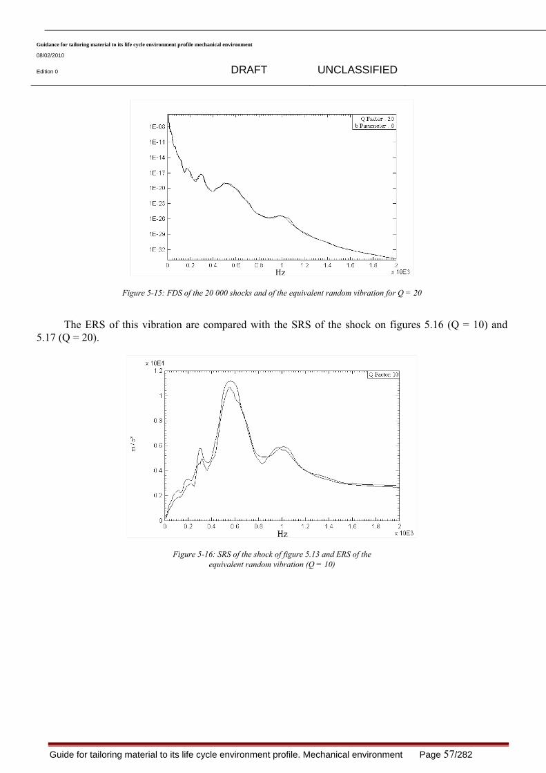
Guidance for tailoring material to its life cycle environment profile mechanical environment
08/02/2010
Edition 0 DRAFT UNCLASSIFIED
Guide for tailoring material to its life cycle environment profile. Mechanical environment Page 57/282
Figure 5-15: FDS of the 20 000 shocks and of the equivalent random vibration for Q = 20
The ERS of this vibration are compared with the SRS of the shock on figures 5.16 (Q = 10) and 5.17 (Q = 20).
Figure 5-16: SRS of the shock of figure 5.13 and ERS of the equivalent random vibration (Q = 10)

Guidance for tailoring material to its life cycle environment profile mechanical environment
08/02/2010
Edition 0 DRAFT UNCLASSIFIED
Guide for tailoring material to its life cycle environment profile. Mechanical environment Page 58/282
Figure 5-17: SRS of the shock of figure 5.13 and ERS of the equivalent random vibration (Q = 20)
Figure 5.18 shows the PSD of the equivalent vibrations calculated for these two values of Q. One notes a substantial difference in the results, the r.m.s. value varying from 398.3 m/s2 for Q = 10 to 345 m/s2 for Q = 20.
Figure 5.18: PSD of the equivalent random vibration determined for Q = 10 and Q = 20
Contrary to the case of a random vibration specification defined to simulate several random
vibrations, equivalence “random vibration – repeated identical shocks” requires to know at the same time the b parameter and the dynamic amplification factor of the structure.

Guidance for tailoring material to its life cycle environment profile mechanical environment
08/02/2010
Edition 0 DRAFT UNCLASSIFIED
Guide for tailoring material to its life cycle environment profile. Mechanical environment Page 59/282
6. STAGE 4 - DRAFTING OF THE TEST PROGRAMME The development of the test programme must normally approach the following elements:
The choice of the standardized method: o The implementation of a standardized method answers a requirement which is to ensure the
test reproducibility; any development of new method must be managed like a project to lead to the objective of validation of a new specifically developed method.
o It is thus essential to adopt a standardized method or a method which has been validated specifically
The choice of the test severity
The definition of the test severity supposes the following steps: o synthesis of the agents of environment to be simulated starting from the characterizations
of the agents of environment selected, by using the specific methods of synthesis to each agent; one will also take into account the particular effects resulting from a combination of several agents of environment,
o transformation of the synthesized environment into test severity by taking into account: - the test factor ,
- Limitations imposed by the test facilities (realizable combination of agents of environment, criteria of appreciation, etc),
- Procedures existing in the standards (ensuring the reproducibility of the tests),
- State of control of art in the simulation of the environment considered,
- Possibly, of the preferential severities suggested by the standards, The choice of the sanction: it is presented to the § 6.2.6
The organization of the test program (sequence of the whole of all the tests) led to seek the best
compromise between: a minimal cost, obtained by successively by carrying out all the tests of each axis without swing
of the shaker from horizontal to vertical or reverse, a good representativeness, by chronologically carrying out each shock and each vibration
according to the three axes, which can allow, at the time of an incident on the material tested, to determine more precisely the origin of it.
6.1. Severities of the tests appearing in the normative documents
One reviews severities of the tests appearing in the AECTP 400 and one brings comments on their contents:

Guidance for tailoring material to its life cycle environment profile mechanical environment
08/02/2010
Edition 0 DRAFT UNCLASSIFIED
Guide for tailoring material to its life cycle environment profile. Mechanical environment Page 60/282
The appendices of the AECTP 400 propose test severities to be used at the beginning of a program in the absence of measurements of the real environment. The part “Method 401 Vibrations” comprises appendices presenting initial test severities.
As example, one can consider the appendix A concerning the wheels vehicles: The corresponding environment belongs to the class “broad band random vibrations” One gives a rolling profile consisting in: a common transportation wheels vehicle with noted V1, an all terrain wheels vehicle noted V2, a two wheels trailer noted V3.
The duration of test and the corresponding distance are given (amount of km): V1: 75 min (60 min represent 4000 km) into vertical and 180 min into transverse or longitudinal
(60 min represent 1609 km) V2: 40 min/axis (40 min represent 805 km) V3: 32 min/axis (32 min represent 52 km)
The PSD of corresponding accelerations are given. Concerning V1, the data come from measurements made on the transportation bed of various
vehicles having a different number of axles, with various types of suspension (blades or air) and various reports/ratios of loading. One considered the envelope of the PSD of all these cases. The variability of the material is not mentioned These PSD do not correspond directly to the recorded data but were affected by an exaggeration to reduce the time of application. (Model of acceleration not specified in the appendix). A1 figure of the AECTP comes from DEF STAN 0035 and MIL STD 810.
Concerning V2, the grounds on which the measurements were taken are representative of military
operations terrains; they include the paved roads, dashboard and the bumps and irregularities of terrain. Various speeds were realized and the loading was of 75% of the nominal load. Various points of measurement were considered on the platform of the vehicle, in the normal zones of installation of the transported materials. The final spectrum comes from a combination of all these cases. The PSD doesn’t correspond directly to the recorded data but were affected by an exaggeration factor to reduce the time of application. (Model of acceleration not specified in this appendix). A2 figure comes from the ITOP 1-2-601 and other sources.
Concerning V3, measurements come from readings taken on the surface of installation of the
secured loads on various trailers with 2 wheels, having one or two axles. The all terrain tracks include the paved roads, dashboard, and the bumps and irregularities of terrain. Various speeds were implemented and the loading was of 75% of the nominal load. The data were not affected by an exaggeration factor.
This way of proceeding brings us to the following remarks: how the envelopes are they realized? If it is with the hand, the effective value will be
unnecessarily too high, the value of the b parameter in the reduction of duration applied for the vehicles to wheel is not
specified. the variability of the material under test is not taken into account. As regards the variability of the environment, one considers the envelope of all the
measurements:

Guidance for tailoring material to its life cycle environment profile mechanical environment
08/02/2010
Edition 0 DRAFT UNCLASSIFIED
Guide for tailoring material to its life cycle environment profile. Mechanical environment Page 61/282
o The vehicles taken into account in the development of the envelopes of PSD are not identified; it is thus not possible to exclude the vehicles non representative with the risk of over-application in certain wavebands, or with under-application in the case or the vehicles not covered by those taken into account for the development of the envelope.
o The envelope is not inevitably sufficient to represent the upper limit of the confidence interval on the environment, in particular for the low numbers of measurements
As many tests as of different PSD
6.2. Contents of a test programme
6.2.1. List of applicable methods
The list of the methods to be applied is function of the environment to simulate, tailored or contractual severities and the required objective.
If certain situations are not covered by the booklets, the test program specificator can work out new
methods, or modify and adapt the existing methods according to his objectives, on the condition of guaranteeing the reproducibility of the procedure corresponding.
6.2.2. Choice of the test procedures
Each method comprises one or more procedures which apply to the various situations. The choice of the procedure is carried out in function:
Of the state of the material, Of the configuration of the material, Of the characteristics of the environment to be simulated, Of the sensitivity of the material to the actuating quantities, Of the existence of the test facility, Of the corresponding cost.
6.2.3. Determination of test severities
Severities of test are established to leave: Of the sought objective, Of the data processing results obtained at step 3 affected by a coefficient of guarantee to cover
uncertainties due to the statistical character of the data and of their treatment Of initial severities to apply after synthesis with other severities rising from step 3. Of the transformation of the environment selected to simulate (fine stage 3) in severity of test per
application of a factor of test.
6.2.4. Tests chronology
The chronology of the tests is established by taking account of the following criteria:

Guidance for tailoring material to its life cycle environment profile mechanical environment
08/02/2010
Edition 0 DRAFT UNCLASSIFIED
Guide for tailoring material to its life cycle environment profile. Mechanical environment Page 62/282
required objective chronology of the agents of environment in the life profile destructive capacity of each test, effects of synergy of 2 simultaneous agents of environment, cumulative Effects of the tests, number of specimens of the material under test.
6.2.5. Amount of specimen under tests
The test programme must specify the number of specimens subjected to tests , as well as the list of tests that each one of them must undergo.
6.2.6. Sanctions 6.2.6.1.Introduction
The severity of the test being fixed, it is important to specify the state of the material during and/or after the test.
In certain cases, it is not possible to admit any derives from the aspect or the operating performances, when this drift is likely to compromise the success of the mission.
In other cases on the contrary, certain drifts, even certain failures, can be tolerated if they do not have a direct incidence on the success of the mission, either because they do not compromise really the exploitation of the material, or because they can be the subject of a simple operation of corrective maintenance.
The purpose of the code of sanction is to establish a graduation in the definition of the state of the
material during and/or after the test since the state where no drift of its characteristics is allowed until that where only a minimum service can be assured.
It is not possible, within the framework of a general standard, to define with precision the
acceptable state of the material after the test. The criteria of examination hereafter can be specified in the test routine.
6.2.6.2.Criteria of examination
The examination of the material is practiced according to three criteria: the apparent state of the material results from its aspect, the possibility of access to the
components and its comfort of operation. This examination can be accompanied by the expertise on the internal state of the material,
the material safety (reference letter “E”) The material safety results from the dangers that the material can make run to the personnel or the surrounding materials because of its state, either during the test or later on. This safety is determined by the value of a certain number of parameters whose variation during the tests can possibly be allowed within certain limits if it does not lead to the appearance of a risk of disaster (wound, electrocution, explosion, fire, flooding, etc.); a later repair will have to then bring back these parameters to their initial value or an agreed value.
Operation (reference letter “F”)
Guidance for tailoring material to its life cycle environment profile mechanical environment
08/02/2010
Edition 0 DRAFT UNCLASSIFIED
Guide for tailoring material to its life cycle environment profile. Mechanical environment Page 63/282
The nominal specific good performance of the material is described by its technical specification. In certain cases, the good performance can be faded by the test, while ensuring of the acceptable minimal performances in servicing. These minimal performances are, if they implicit, are not fixed by the technical specifications. The examination of the specific operation of equipment during and/or after the test is generally carried out by comparison with initial specific operation on the basis of number certain of significant parameters possibly specified by the test programme.
The assistance with the choice of the sanction of the test is described in appendix 8.13.
6.3. Need and calculation of the test factor
6.3.1. Necessity of the test factor
In order to obtain a specified reliability level, the necessary mean resistance value can be defined by multiplying the mean ( )rμ by the coefficient of guarantee CG > 1.
Generally, this CG value is obtained by carrying out withstand test on a certain number of specimens reputed to be identical to the material or to the equipment considered. For obvious economic reasons, the possible test number is necessarily limited and the variability of sampling leads to a statistical estimation of this mean value.
So, the aim of the tests consists in checking that the coefficient of guarantee, as well as the expected reliability is reached when a prescribed probability level is obtained. If an interval confidence can be attached to the punctual estimation of this mean value or better, if one can know its statistical distribution, this mean value will be thus well associated to a probability level.
According to the retained probability level, possible number of tests and coefficient of variation characterizing the resistance distribution, one can define a test factor FE >1. This one, as a multiplying coefficient of the coefficient of guarantee CG, can be interpreted as a factor increasing the test severity.
Practically, in order to reach the necessary reliability level with a given probability, the resistance level
resulting from the tests must be at least equal to the product (FE.CG).
6.3.2. Test factor calculation for the normal distribution:
It is supposed that the resistance is represented by a normal distribution knowing only its coefficient of variation (CVr).
In order to estimate the unknown mean value ( )rμ one carries out (n) tests allowing to obtain the arithmetic mean value (m) of this sample of size (n). In fact, this arithmetic mean value (m) is only an approximate value of ( )rμ and it is necessary, on one hand, to correct it for eliminating its bias and, on the other hand, to associate it dispersion measures (i.e. its variance).

Guidance for tailoring material to its life cycle environment profile mechanical environment
08/02/2010
Edition 0 DRAFT UNCLASSIFIED
Guide for tailoring material to its life cycle environment profile. Mechanical environment Page 64/282
For (CVr < 1/3) and (n = 1, 2, 3...), one can show that the unknown mean is a random variable, practically distributed according to a normal distribution whose mean is estimated starting from the method of the maximum likelihood [PIE 07]:
( )2 2
r r r r2r
mˆ CV ;n 1 4 k CV 1 CV 12 k CV
⎛ ⎞ ⎡ ⎤⎛ ⎞⎛ ⎞⎜ ⎟μ ≅ + + −⎢ ⎥⎜ ⎟⎜ ⎟⎜ ⎟ ⎜ ⎟⎝ ⎠⎢ ⎥⎜ ⎟ ⎝ ⎠⎣ ⎦⎝ ⎠
[6.1]
With: ( )n
ii 1
m 1/ n x=
= ∑ and ( ) ( )k n 1 1 n= + is a bias correction factor; this one permits to obtain an
explicit solution acceptable in case of a test number such as n>1 or 2≥n . Since the test factor is defined as a relative value, one can standardise the arithmetic mean as m =1.
To this estimator of the mean, one can associate a minimal variance corresponding to the Cramer-Rao bound which leads to obtain the coefficient of variation:
( )r r
2rr
ˆ CVn
ˆn 1 2 CV
σ≅
μ ⎛ ⎞+ ⋅⎜ ⎟⎝ ⎠
[6.2]
For a prescribed exceeding probability p % , or equivalent for a probability not exceeding ( )100 p%− , one can determine the test factor nFE by using the quintile corresponding to the standardized normal distribution such as defined in chapter 5.7.1, that is :
( )1r
n2r
CVFE 1 100 p %
n 1 2 CV
−≅ + ⋅Φ −
⎛ ⎞+⎜ ⎟⎝ ⎠
[6.3]
The abacuses 4-a, 4-b, 4-c of appendix 8.2 make it possible to obtain approximate values corresponding to
three exceeding probability levels: p = 5, 10 and 20%, that is ( )1
95%−
Φ ; ( )1
90%−
Φ ; ( )1
80%−
Φ .
Numerical application: Let us suppose that: CVr = 1/3, n=2 and (100 – p %) = 95% Then rμ̂ = 0.958, ( )r rˆ ˆ 0 .213σ μ = , ( )1 95% 1.645−Φ = , hence: nFE (2) = 1.351 (bias is about 4%)
6.3.3. Test factor calculation for the log-normal distribution

Guidance for tailoring material to its life cycle environment profile mechanical environment
08/02/2010
Edition 0 DRAFT UNCLASSIFIED
Guide for tailoring material to its life cycle environment profile. Mechanical environment Page 65/282
In this case, the estimator which coincides well with numerical simulations is a log-normal distribution which has the same average distribution of reference and a variance equal to the variance of the distribution of reference divided by n. Then, starting from the quintiles of the standardized normal (i.e. table 1 of chapter 5.7.2.), it is possible to determine the resistance value corresponding to an exceeding probability (p %). This step makes it possible to define explicitly the test factor lnFE , as it follows:
( )2 1r
ln 2r
exp Log 1+ CV / n . 100 p %
FE
1+ CV / n
−⎡ ⎤⎛ ⎞ Φ −⎢ ⎥⎜ ⎟⎝ ⎠⎢ ⎥⎣ ⎦
=⎛ ⎞⎜ ⎟⎝ ⎠
[6.5]
The abacuses 5-a, 5-b, 5-c of appendix 8.2 make it possible to obtain the values corresponding to
three exceeding probability levels: p = 5, 10 and 20%, that is ( )1
95%−
Φ ; ( )1
90%−
Φ ; ( )1
80%−
Φ . Numerical application: Let us suppose that: CVr = 1/3, n = 2, (100 – p%) = 95%, ( )1 95% 1.645−Φ = Hence: ( )lnFE 2 = 1.427
6.3.4. Test factor calculation for the Weibull distribution: In case of the Weibull distribution, its coefficient of variation (CVr) is connected non-linearly to its shape parameter ( )rβ . When this last one is imposed, taking into account the power transformation of the reduced variable, the problem leads to consider the mean value of an exponential distribution, starting from a sample of size (n).
In these conditions, the scale factor ( )rη of the Weibull is a random variable distributed according to a Gamma distribution. It is the same, except for a coefficient, for the searched mean value.
If like previously, one introduces the quintile of the standardized normal distribution
( )%1001 p−Φ− corresponding to a non-exceeding probability (100-p%), the test factor can be written [PIE-2005]:
321r r
wCV CV
FE 1 . ( 100 p %)3 n 3 n
−⎡ ⎤⎛ ⎞ ⎛ ⎞⎢ ⎥≅ + Φ − −⎜ ⎟ ⎜ ⎟⎜ ⎟ ⎜ ⎟⎢ ⎥⎝ ⎠ ⎝ ⎠⎢ ⎥⎣ ⎦
[6.6]

Guidance for tailoring material to its life cycle environment profile mechanical environment
08/02/2010
Edition 0 DRAFT UNCLASSIFIED
Guide for tailoring material to its life cycle environment profile. Mechanical environment Page 66/282
The abacuses 6-a, 6-b, 6-c of appendix 8.2 make it possible to obtain approximate values
corresponding to three exceeding probabilities: p = 5, 10 and 20%, that is ( )1
95%−
Φ ; ( )1
90%−
Φ ;
( )1
80%−
Φ . Numerical application Let us suppose that: CVr = 1/3, n = 2, (100-P%) = 95%, ( ) 645.1%951 =Φ− Hence: ( )wFE 2 = 1.417
Note: When one has only one measurement of the environment, it is of use to apply a default guarantee coefficient selected according to the experiment. If the value selected is for example equal to 1.2 (applied to the temporal signal), that corresponds:
- by supposing that the laws of distribution of the environment and resistance are lognormal, - and that the probability of failure is equal to 10-3, with a coefficient of variation of resistance close to 6%. It is pointed out that this coefficient of variation remains lower than 8% for the majority of metallic materials and that it can even sometimes exceed this value. For a probability of failure of 10-6, this coefficient of variation passes to 3.8%. The use of a coefficient of flat-rate guarantee can thus prove too optimistic.
6.4. Reduction of the test duration
In the case of the method ERS/FDS, the definition of an endurance reduced duration test of equal fatigue damage is based on the expressions of the damage deduced from the Basquin law. For sinusoidal vibrations, one has as follows:
bmax
bmax
bzNConstantezTf
CK
D == [6.7]
Where relative displacement zmax is proportional to the constraint, which is to say with the amplitude of the input mx&& .
The number of cycles N being equal to N f T= , two vibrations of amplitude mm 1x&& and m 2x&& respective durations 1T and 2T produce the same fatigue damage if:
1b
1m 2 m1
2
Tx xT
⎛ ⎞= ⎜ ⎟
⎝ ⎠&& &&
[6.8]

Guidance for tailoring material to its life cycle environment profile mechanical environment
08/02/2010
Edition 0 DRAFT UNCLASSIFIED
Guide for tailoring material to its life cycle environment profile. Mechanical environment Page 67/282
In the case of a random vibration, one has in a similar way: 1
b1
eff 2 eff 12
Tx xT
⎛ ⎞= ⎜ ⎟
⎝ ⎠&& &&
[6.9]
This rule can be also deduced directly from the Basquin relation bN Cσ = .
It uses the same assumptions as those considered in a more implicit way in the duration reduction
rules provided by the older standards. It utilizes the parameter b with the same difficulties of its value choice in the case of structures
made up of several materials. This parameter is fixed at a certain value in these standards, with the consequences of an over-
test1(if steel or aluminum structures when having chosen b = 5) or of an under-test2 (if electronics when having chosen b = 8) systematic, whereas it can be selected in a more relevant way with the ERS/FDS method where choice is made according to the nature of materials indeed present in the studied material.
6.5. Validation of the time reduction
The ERS can be used to directly write (in the place of the FDS) a specification when the duration of the vibration is of no importance (only respect of the largest constraint under test),
The ERS wrapping ERS of several events of a life profile can be used to calculate a test specification defined by a PSD when one can consider that the most important risk is a rupture due to a too large constraint.
The method consists in seeking the characteristics of a PSD which produces the same ERS as that of
the profile of life, by fixing one arbitrary duration, knowing that the ERS is a spectrum not very sensitive to vibration duration [LAL 09e].
It is desirable that the duration of the specification thus defined be small, to the maximum equal
with that of the most severe event of the life profile, in order not to risk a rupture by fatigue which would not be representative. The goal of the test is here simply to check that the material resists the strongest levels met in the real environment.
The justification of the reduction of the duration is carried out here while resting on the ERS, which
make it possible to check that the constraints produced by the shocks are of the same order of magnitude or larger than those created by the random vibrations of reduced duration. The use of the ERS is in general sufficient. However, this comparison could be realized in a more precise way using the URS.
1 Over-test: Too high severity of test compared to the objective of the test 2 Under-test: Severity of test relatively low compared to the objective of the test.

Guidance for tailoring material to its life cycle environment profile mechanical environment
08/02/2010
Edition 0 DRAFT UNCLASSIFIED
Guide for tailoring material to its life cycle environment profile. Mechanical environment Page 68/282
Use of the ERS to validate the reduction of duration. The process in four stages used to determine a specification results calculating the FDS of all the
vibratory environments of the life profile of the concerned material and in deducing by envelopes (for the situations in parallel) or by additions (for the situations in series) a FDS representative of the fatigue damage created by the life profile. The following step consists in seeking a PSD of given duration, in general smaller than the duration of the real environments, which has a FDS wrapping (very near) of that of the profile of life (cf figure 6.1).
Figure 6-1: FDS of the profile of life and the specification
On the basis of the PSD evaluated in this way, it is necessary to recalculate the ERSs and FDSs in order to estimate the quality of the obtained specification. The FDS is thus compared with the FDS of the complete life cycle profile. If the differences are too large, the number of definition points of the PSD or the frequency values of the selected points may be modified.The ERS is compared with the life cycle SRS to evaluate the effect of the duration reduction with respect to the complete life cycle. In order to simplify the presentation, the notation ERSSP will represent the extreme response spectrum of the specification, and ERSLP that which results from the life cycle profile environment (reference). Several situations are possible:
SRS > ERSSP > ERSLP (cf figure 6.2).
Figure.6-2: acceptable reduction of the duration

Guidance for tailoring material to its life cycle environment profile mechanical environment
08/02/2010
Edition 0 DRAFT UNCLASSIFIED
Guide for tailoring material to its life cycle environment profile. Mechanical environment Page 69/282
This is the ideal situation. The ERSSP is greater than the ERSLP due to the reduced duration, but is smaller than the SRS: under test conditions, the equipment will not be submitted to instantaneous levels greater than those under the real environment. The specification comprises a random vibration and a shock defined on the basis of the SRS of the life cycle profile (simple type shock or SRS itself).
ERSSP > SRS > ERSLP (cf figure 6.3).
Figure 6-3: exaggeration factor too important: increase the test duration
The ERSSP is greater than the SRS. Two attitudes are possible: - maintain the specification with its duration (reduced), and by so doing taking the risk that a
problem may occur during the test which could be due to instantaneous stress levels to which the equipment would not normally be submitted in its useful life. This choice can be justified by the need to considerably reduce the test when the real environment duration is great. However, if an incident occurs during the test, this does not necessarily show that the equipment does not comply. An envelope spectrum shock of the ERSSP right at the beginning of the test might be envisaged in order to check that the equipment is able to withstand the stress to which it will be submitted artificially under vibration (without being damaged). There is no need to simulate the shock that corresponds to the SRS.
- select a greater duration in order to return to the previous case. ERSSP > ERSLP > SRS (cf figure 6.4).

Guidance for tailoring material to its life cycle environment profile mechanical environment
08/02/2010
Edition 0 DRAFT UNCLASSIFIED
Guide for tailoring material to its life cycle environment profile. Mechanical environment Page 70/282
Figure 6-4: The reduction of duration always presents a risk
Real environment shocks are fairly weak in amplitude compared to vibrations and cannot clear the duration reduction. In this instance it is advisable not to reduce too much the duration. It is also possible to start with an envelope spectrum shock of the ERSSP for the same reasons as mentioned earlier. There is no need to perform a shock that covers the SRS of the real environment.
ERSLP > ERSSP (cf figure 6.5).
Figure 6-5: Too large duration
The vibrations of one of the life cycle profile events are undoubtedly much stronger than the other vibrations, and do not last very long. The specification is influenced mainly by this event. If this specification is applied for a reduced time compared to the duration of the whole life cycle profile, but for a longer time than that of the overriding event, it will result in the test duration being extended and therefore to the levels being reduced. In this case, the test duration must be reduced again until the two spectra are very close, the ERSSP slightly enveloping if at all possible the ERSLP.
An illustration of this approach is presented in the treatment of the example in appendix 9.

Guidance for tailoring material to its life cycle environment profile mechanical environment
08/02/2010
Edition 0 DRAFT UNCLASSIFIED
Guide for tailoring material to its life cycle environment profile. Mechanical environment Page 71/282
6.6. Return to PSD starting from the FDS
The calculation of the characteristics of a PSDA which produces over a given duration the same FDS that the FDS of the life profile can be done in a simple way by iteration:
Choice of N points on the FDS of the life profile , Generation of a PSDA of constant amplitude on the frequencies domain of the FDS at the
frequencies chosen above, Calculation of its FDS, Calculation at each frequency of the ratio R between the FDS of reference (life profile ) and the
FDS of the PSD, Readjustment of the amplitude G of the PSDA at each frequency by making the product 2/ bG R .
6.7. Return to PSD starting from the ERS
The calculation of the characteristics of a PSDA which produces over a given duration the same ERS that of the life profile can be done according to the same process. The readjustment of the amplitude G of the PSDA at each frequency is obtained here by making the product 2G R where R is here the ratio of the ERS at a given frequency.
6.8. Notice on the specification of the shocks by a SRS
The shaker control systems make it possible to realize the shocks on a shaker starting from a specified SRS. The calculator of the system built starting from this SRS a temporal signal which it sends on the shaker. This signal is constitued of the sum of simple components of forms (damped sines, WAVSIN, ZERD, wavelets…) of which the characteristics (amplitude, logarithmic decrement or damping coefficient, number of periods in the wavelet form …) are estimated by several iterations so that the SRS of the made up signal is close to the specified SRS.
If no precaution is taken, the signal thus built can have characteristics very different from the shocks
at the origin of the specification, with a much lower amplitude and a larger duration often approximately 10 times.
Although a priori the equality of the SRS is sufficient (it is the comparison criterion of the shocks severity), the test program specificator often imposes a complementary parameter, in general a maximum duration of the shock carried out. To obtain this result, the method can consist in being unaware of the first points of the SRS since it is them which lead to the components of greater duration.
Another manner of removing the problem would be to specify the shock by its SRS traced until a sufficiently high frequency to reach the static zone in which the amplitude of the SRS tends towards that of the shock. The specified SRS calculated under these conditions would impose in fact the amplitude of the shock and would lead to a duration closer to the real one.
6.9. Possibility of splitting a band in several (generally 2) sub-bands

Guidance for tailoring material to its life cycle environment profile mechanical environment
08/02/2010
Edition 0 DRAFT UNCLASSIFIED
Guide for tailoring material to its life cycle environment profile. Mechanical environment Page 72/282
When passing from the 3rd step of the tailoring process (synthesis of the environments to be simulated) to the 4th step (test programme), it should be checked that elaborate tests severities are realizable on the shakers of the test laboratories. In the case of a random vibration test, it can arrive that the temporal induced peak value (at least 2.3 times the effective value, because the majority of the standards impose a tolerance on the distribution of the instantaneous values at least up to 2.3 standard deviations) exceeds the usual limit of 100 g temporal that generally the laboratories do not want to take too many risks of degradation of their shaker field coil.
Only” induc’t a ring shakers” of the manufacturer Unholtz Dickie) accept temporal peak values of 600g but these shakers are rare.
In the case where a specified test leads to a temporal peak value exceed 100 g, one can then have to split the specified test band under adjacent sub-bands. Is this acceptable?
The answer to this question will depend on the material under test and the expected modes of
failure. If the equipment under test is purely structural (not electronics, no mechanism, no optics), one will be able to cut out under sub-bands of such kinds that the point of cut is sufficiently distant (at least 0.6 by in lower part and 1.4 with the top of a structural mode), to avoid making disappear the effects of the coupling between 2 coupled modes. It does not remain about it less than the effective efforts of interface, wrenching, etc can be affected by the fact that the acting modes are separate in 2 sub- bands. It will be necessary in such a case to carry out a modelling of the structure in order to determine the corrective factors on the peak values to apply. The experimental validation could possibly be prevented if a modelling approach makes appear sufficient margin.
In the case where an electronics component, or a mechanism, or an optic equipment, a preliminary risk analysis must be made to make sure that no component has sensitivity to the peak value. This demonstration will be convincing only on the basis of sufficient experience feedback for identical components.
One will also validate this cutting by comparing the ERS and FDS of the specification and the test based on the sub-bands thus carried out.
6.10. Test Rigs
6.10.1. Frame of loading/testing machine
The simplest assembly of the test is a monoaxial testing machine, or it load is applied to the material under test thanks to a mass of reaction. It can be used for simulations of tests on components in the case or the loading relates to a component. These machines can implement a linear actuator for loadings in traction/compression or inflection, or a actuator in torsion for loadings of torsion.
Note: it is not a very usual test and no method describes it
6.10.2. Tables of generator of vibrations
A table of tests on a generating whole of vibrations consists in its upper part of a rigid plate guided by stages and pulled by force of an electrodynamics or electrohydraulic origin which can drive the table

Guidance for tailoring material to its life cycle environment profile mechanical environment
08/02/2010
Edition 0 DRAFT UNCLASSIFIED
Guide for tailoring material to its life cycle environment profile. Mechanical environment Page 73/282
according to 1 or several axes, or of rotation around one, two even 3 axes. When the movements take place along 3 axes and around the 3 axes, one speaks about movement according to 6dof.
6.10.3. Specific loading but through a flexible coupling
The loading can be applied to the material under test via a flexible device making fixed at the generator of vibrations at an end and at the material under test at the other end. The flexible connection allows an axial mono loading and avoids the application of rotations and minimizes the couplings with the 2 other axes. The material under test can be supported with structure via its nominal modes of assembly, or is embedded or supported by a flexible device.
6.10.4. Mono excitation axial and multi point
An axial mono installation but multi point entrance to several generators of vibrations placed in parallel. In example one can quote two generators of vibration coupled to test loads of great dimension (missile, container of missile), a whole of four generators of vibration using a whole of guidance to sleeve bearings composed of four “posters” (sleeve bearing guidance, one by generating whole of vibrations) to vibrate of the vehicles with wheels by attacking for example each wheel separately, or to represent the loadings of the aerodynamic efforts. The material under test can be embedded locally (wing of plane or fuselage) or free (wheel of vehicle).
6.10.5. Excitation multiaxial and Mono point
An axial system multi and mono point of excitation implements several generators of vibration
acting according to two or three of the rectangular tri directions with specific points of application. This is implemented in the cases or a multi axial environment applies punctually to the material under the real condition of uses.
As example one can quote the wheel of a vehicle, the rotor of head of a helicopter, and the point of
fixing of a missile in carrying under plane. The axial system multi and mono point of excitation requires flexible connections to authorize the degrees of freedom necessary in the 3 orthogonal directions. There can be coupling between the axes that one of three (at least the) generating ones of vibration excite simultaneously.
6.10.6. Excitation multiaxial and multi point
An axial system multi and multi not of excitation relates to the cases or of the distinct entries are excited according to different directions. For example, aerodynamic loading in phase propelled of a missile, or aerodynamics effects on the equipment of the missile by attack in 2 flexible entries with a generator of vibrations per entry.
6.11. Relative questions with the triaxial aspect of the real environment
In reality the vibratory excitations are triaxial and it happens that they apply in several entrance points of the system (case of a vehicle by the 4 points of connection on the ground for example).

Guidance for tailoring material to its life cycle environment profile mechanical environment
08/02/2010
Edition 0 DRAFT UNCLASSIFIED
Guide for tailoring material to its life cycle environment profile. Mechanical environment Page 74/282
For the level of the associated specification and test facilities, it is advisable to differentiate the
triaxial excitations applied in a point or several points from the system.
6.11.1. Triaxial excitation mono point
If it is considered that the mechanical system behaves in an isotropic way compared to the damage, i.e that the internal connections and the secondary excitations of the system are neglected, it is possible to calculate the damage produced by a triaxial excitation in all the directions of space.
The damage produced by a triaxial excitation, can be given by the projection of measurements of excitation in X, there, Z in each direction of space starting from the angle of raising α (in the horizontal plane compared to X) and of the angle of elevation Β (compared to the horizontal plane).
From the distribution of the damage in the various directions of space, there exist 2 possible choices:
the damage is mainly present on axes X, there, Z of the system. In this case, it is possible to use like test facility a table of generator of mono vibration centers (cf § 6.10.2). If need be, one will apply a factor of increase to the level of the specification of tests to obtain a damage raising in all the directions of space,
the damage is distributed in all the directions of space (case of an automobile seat). In this case, it is advisable to use a multiaxis system of excitation which can cover up to 6 degrees of freedom (translation and rotation around the 3 axes) to obtain a representative test. The specification of test is carried out in the temporal field in order to thus control the phase the direction of the triaxial excitation. Techniques exist which make it possible to specify accelerated three-dimensional tests which respect the FDS in all the axes (cf [VIV 06]).
Note: The choice of the parameter b in the employment case of a law of Basquin has a real influence on the distribution of the damage in the various directions of space. The damage will be rather present on the main axes of the system for a b important (b>8) and rather distributed for a b weak because the influence on a direction forming an angle α with the main axes will be attenuated of a coefficient (cos.α) B. At the opposite, the damage will be distributed in a more homogeneous way for a b weaker.

Guidance for tailoring material to its life cycle environment profile mechanical environment
08/02/2010
Edition 0 DRAFT UNCLASSIFIED
Guide for tailoring material to its life cycle environment profile. Mechanical environment Page 75/282
Figure 6-6: calculation of the damage produced by a horizontal excitation in any point of a plan for 2 choices of parameter b in the employment case of a law of Basquin: b = 4 (left) and b = 8 (right-hand side)
6.11.2. Mono axial or triaxial excitation multipoint:
A triaxial or mono axial excitation multipoint introduces important triaxial constraints in any point of the system. For example, an excitation primarily vertical, but shifted in time under the nose gears and back of a vehicle (passage of a back of ass) led to triaxial requests in any point of this one. Two choices are possible:
to use a test facility adapted, i.e a multipoint system multiaxial (cf § 6.10.6) or mono axial multipoint (cf § 6.10.4) according to the nature of the excitation in each point,
to break up the system into under systems until being able to consider that only one entrance point is representative.
6.12. Mechanical environments low frequency - static field - quasi-static
6.12.1. Position of the problem
The tailoring process for mechanical environment also applies to the static and quasi-static stresses. The life profile consists in situations where the material is subjected to static accelerations or very low frequency acceleration, which it is necessary to identify and quantify. The specifications are generally expressed in the form of torques of efforts to the interfaces, and in the form of field of accelerations brought back to the CoG. In the case of the missile systems, the values result generally from simulations by FEA very early in the development (phase of feasibility). These simulations by FEA are in certain case the exchange object of models between industrialists, to take into account the dynamic behavior of the missile integrated into the carrier which can be a terrestrial vehicle, a naval structure or an airplane. The structural design takes account of the enveloping case, known as dimensioning (sizing?), so that the margin was higher or equal to 0 at Extremal Charge which means: without plastification or unrecoverable deformation deteriorating the performances when the material is subjected to the maximum environment likely to be met (the standard dedicated to these aspects is the standard AIR 2004 in France). The fatigue damage related to these static accelerations or low frequency acceleration must also be analyzed: part “low number of cycles” of the Whöler curve characterizing materials, low number of cycles, and great amplitude of constraint. A structure can slightly have locally constraints above the yield stress provided that the number of cycles does not lead to rupture by oligocyclic fatigue.
It should be noted that the specifications in the static and quasi-static field takes into account the six degrees of freedom, translations and rotations: field of acceleration with angular accelerations, torques of efforts with six components: normal effort, sharp efforts and moments.
The spectrum of the mechanical environment in the frequency domain is broad ; it is cut out in several sections for which the sources of excitation, the effects induced and the types of problem met as well as the associated test facilities to reproduce in laboratory these environments are different. In the frequency low part of the spectrum, the border between the “static or quasi-static” field and the “vibrations and shocks” is not always easy to distinguish. These two fields call upon methodologies, standards of the different test facilities, whereas physical reality is without border.

Guidance for tailoring material to its life cycle environment profile mechanical environment
08/02/2010
Edition 0 DRAFT UNCLASSIFIED
Guide for tailoring material to its life cycle environment profile. Mechanical environment Page 76/282
The purely static field is characterized by accelerations of null frequency of which here some current examples:
Under the effect of gravity the structures undergo constraints at the time of the phases of handling Load factors during the plane maneuvers Acceleration of a missile during the shooting under the effect of propulsion engine.
Two different types of test meet the needs for validation in the purely static field: Tests out of centrifugal machine to reproduce a field of constant acceleration, these tests are
generally made on the level “electronics components” Tests with hydraulic actuating cylinders to reproduce torques of effort, these tests are made on
the level “structure”.
In the quasi-static field the system behaves almost as in the static field; the modes of rigid body are prevalent. In practice the terminals of the quasi-static field are extended until including the first modes of elastic strain. In this quasi-static field, the environment has frequential contents low frequency in comparison with the structure or excited mechanical system.
In the static field the relation γMF = expresses that all the mass of the system subjected to acceleration takes part to generate efforts and constraints. That remains true when the frequency of excitation is lower and is decoupled from the first resonance of the system. In this case the system behaves like a rigid body and it is easy to be reduced by equivalence to the purely static field. On the other hand, when the environment has frequential contents which include partially or completely the first resonances of the system, equivalence carried out dynamics-statics when one wishes to specify static loading cases to cover a dynamic environment is not more commonplace and requires an approach by modeling FEA. The higher the frequency is and the local modes will be excited bringing into play increasingly low dynamic masses while moving away from the relation γMF = .
Let us take the case of a embed-free beam for which we have: an effective mass for the first bending mode representing 61% of the total mass, and that of the
second mode 19%. an acceleration of 10 g fixed at the frequency of the second mode will have less effect in terms of
constraints to embedding, than a static acceleration of 10 g. the deformation of the first mode of inflection of a fixed beam is different from the deformation
under a static field of acceleration. In dynamics the effect of the angular accelerations induced of the transient moments in the
sections M Jϑ= &&
The process of specification and the logic of validation for a system meeting a dynamic dimensioning environment whose spectrum includes until the first elastic modes is an integrate calculation-tests process. It is the case for example missiles integrated under planes subjected to the landing shocks , or the missiles integrated on ships subjected to the “grenadage” shocks . This process can lead to different type of ground tests :
Tests reproducing or wrapping torques of efforts met at the time of the dynamic stress Tests reproducing or wrapping SRS without however generating efforts in the inappropriate.
structures Tests ( experimental modal analysis, characterization of stiffnesses,…) required with for
objectives of models tuning and validation .

Guidance for tailoring material to its life cycle environment profile mechanical environment
08/02/2010
Edition 0 DRAFT UNCLASSIFIED
Guide for tailoring material to its life cycle environment profile. Mechanical environment Page 77/282
Examples of the missiles integrated under plane subjected to the shocks of landing (the same
process “test-calculation” is applied to the case of the missiles integrated to frigate subjected to the “grenadage” shocks).
6.12.2. Examples of the missiles integrated under plane subjected to the shocks of landing
The same step test-calculation is applied to the case of the missiles integrated to frigate subjected to the shocks of grenadage.
A FEA model of the plane + missile is necessary to know the entries of the missile and thus to specify and conceive just as necessary. One of the difficulties is that the entries of the missile depend partly on the definition of the missile; an iterative process is thus done during the development to readjust these entries. The logic of validation can be based on static tests to validate the behavior of the structures and on dynamic tests, to generally validate the non structural equipment or to characterize the dynamic behavior.
Exchanges of models between industrialists, in the form of dynamic super-elements (DSE) are
carried out. These condensed models are matrices masses and stiffnesses of reduced sizes representing the dynamic behavior correctly. A condensed model of the missile laucher and missile are integrated into FEA model of the plane to simulate a shock of landing per excitation on the level of the plane landing gear. The entries of the missile obtained by simulations can be expressed in several forms: torques of efforts to the interfaces, field of accelerations at the CoG, temporal of efforts and accelerations at the interface, SRS calculated from these temporal of acceleration at the interface. These entries are then applied to non-condensed FEA models of the missile from where the efforts are deduced, accelerations, and constraints in the most critical zones. The logic of validation will be founded on these results.
By static tests the zones will be only tested where the margins released by calculation are weak. The
cases of loading of these tests are defined to reproduce or wrap the torques of effort in the sections and the connections. These tests are generally carried out until rupture in order to know the margins. The results are also used to characterize the stiffnesses under high loadings and take part in the validation of the models.
The dynamic tests can be initially made on structural nonfunctional material within the framework
of flight clearance in order to characterize the dynamic behavior and validate the models. They are then carried out on functional materials within the framework of the qualification. FEA models make it possible to apply the real environment such as it is without being confronted with the limitations of the test facilities: the material is thus requested “virtually” with an environment which starts to 0 Hz with several entries (translations and rotations at the multiple points of interface) simultaneously. Simulations by FEA highlight that it would be interesting to carry out certain tests using multi-points or multi axis vibration test control. Until now, all the tests in vibrations or shocks are carried out with traditional systems with mono point and mono axis control. Those make it possible to obtain a level specified in a point of the structure or equipment. Responses to the other points not being controlled, they differ from those obtained under the operational conditions. They can all the more differ if rigidities of interface with the frame distort the modal behavior. It was shown that tests carried out with mono-excitation (mono point and mono axis) and a rigid interface can result over-testing (and locally under- test in other points), generating efforts in the junctions up to three times too important. A flexibility of adapted interface makes it possible to restore the modal behavior low frequency. A multi-excitation (multi
Guidance for tailoring material to its life cycle environment profile mechanical environment
08/02/2010
Edition 0 DRAFT UNCLASSIFIED
Guide for tailoring material to its life cycle environment profile. Mechanical environment Page 78/282
points and multi axis) system of control makes it possible to introduce two (or more) different temporal inputs, by respecting the phases, at the various points of interface.
6.13. Representativeness and reproducibility of the tests
The test reproducibility is the faculty of this one of being able to be again carried out accurately in time and space. A test must lead to the same results whatever the place, the means implemented, the operator and the period in time. The key of a good reproducibility is the strict application of the standardized testing method.
It is responsibility for the laboratory of test to ensure itself at the time of the review of contract
which this method of reference is well specified by the customer. In the contrary case, the test laboratory owes stage with the deficiency of the customer by choosing the method which appears to him most suitable. Identification of the testing standardized method figures obligatorily in the test report.
The test representativeness is the faculty of this one to reproduce in test laboratory the modes of
failure which would be observed of operational use, in order to correct them. The representativeness, contrary to reproducibility, is not an objective in oneself. The Just necessary of representativeness is to be sought.
The parameters that will affect this representativeness are: interface or installation conditions with the test facility: mechanical impedance (ratio Forces
injected /velocity produced) at the entry, distribution of the points of interface, nature of the junction elements,
the aspects multi input and multi axes, (cf § 6.10) the degree of representativeness of the mechanical quantities simulated compared to the real
environment (temporal evolution, phase or correlation of the entries, etc) The influential factors on the level of representativeness to be ensured are: proximity of the constraints of environment applied with the limits of design of the material:
more one approaches these limits and better will have to be the representativeness of the test the level of assembly which the failure is awaited: in theory, a mechanical test of environment
should not call into question the high level of assembly (the overall structure), but rather the low level of assembly (a component assembled on a chart in equipment). More the failure relates to high level of assembly and better will have about it to be the representativeness of the test.
The test reproducibility is the faculty of this one of being able to be again carried out accurately in time and space. A test must lead to the same results whatever the place, the means implemented, the operator and the period in time. The key of a good reproducibility is the strict application of the standardized testing method.
It is responsibility for the laboratory of test to ensure itself at the time of the review of contract
which this method of reference is well specified by the customer. In the contrary case, the test laboratory owes stage with the deficiency of the customer by choosing the method which appears to him most suitable. Identification of the testing standardized method figures obligatorily in the test report.
The test representativeness is the faculty of this one to reproduce in test laboratory the modes of
failure which would be observed of operational use, in order to correct them. The representativeness,

Guidance for tailoring material to its life cycle environment profile mechanical environment
08/02/2010
Edition 0 DRAFT UNCLASSIFIED
Guide for tailoring material to its life cycle environment profile. Mechanical environment Page 79/282
contrary to reproducibility, is not an objective in oneself. The Just necessary of representativeness is to be sought.
The parameters that will affect this representativeness are: interface or installation conditions with the test facility: mechanical impedance (ratio Forces
injected /velocity produced) at the entry, distribution of the points of interface, nature of the junction elements,
the aspects multi input and multi axes, (cf § 6.10) the degree of representativeness of the mechanical quantities simulated compared to the real
environment (temporal evolution, phase or correlation of the entries, etc) The influential factors on the level of representativeness to be ensured are: proximity of the constraints of environment applied with the limits of design of the material:
more one approaches these limits and better will have to be the representativeness of the test the level of assembly which the failure is awaited: in theory, a mechanical test of environment
should not call into question the high level of assembly (the overall structure), but rather the low level of assembly (a component assembled on a chart in equipment). More the failure relates to high level of assembly and better will have about it to be the representativeness of the test.

Guidance for tailoring material to its life cycle environment profile mechanical environment
08/02/2010
Edition 0 DRAFT UNCLASSIFIED
Guide for tailoring material to its life cycle environment profile. Mechanical environment Page 80/282
7. RECOMMENDATIONS ON THE CHOICE OF THE VALUES OF THE PARAMETERS
7.1. Choice of the value b
7.1.1. Usual values
In the standards, this parameter however is fixed a priori at a certain value, with the consequences of a over-test (case of the structures out of aluminum or steel when b is fixed at 5) or of a under-test (case of electronics when b is selected equal to 8). One could for example in the case of an electronics component separately validate the electronic case (b=8) and PCB (b=4).
The value currently recommended in the GAM EG 13 Mechanical Appendix General for b is: Alloys of aluminum: 6 to 10 Steels: 10 to 15 Alloys of magnesium: 20 to 25
In a complex material, many types of damage are possible other than the damage by fatigue. For
electronics, when the rupture is due to a fatigue of the mechanical type (for example electrical contacts), the Wöhler curve applies with a parameter b of about 3 to 4. But degradation by corrosion and fretting of the contacts can be important. The equivalences based on malfunctions still miss coherent data.”
The standard MIL STD 810 recommends a value of 7.5 whereas DEF STAN 0035 proposes 5. A value from 3 to 4 is also the case of the roll bearings, electronic component dice and for the
weldings of mechanical structures Recent work leads to values ranging between 4 and 6 for weldings of electronics components CMS
or BGA. In the literature one finds values of b described in tables 7.1 and 7.2.
Material b
Copper Wire
Aluminum Alloy: 6061-T6
7075-T6
Soft Solder (63-37 Tin-Lead)
4340 (BHN 243)
4340 (BHN 350)
AZ31B Magnesium Alloy
9.28 8.92 9.65 9.85 10.5 13.2 22.4
Table7 -1: Some values of b [LAM 80]

Guidance for tailoring material to its life cycle environment profile mechanical environment
08/02/2010
Edition 0 DRAFT UNCLASSIFIED
Guide for tailoring material to its life cycle environment profile. Mechanical environment Page 81/282
Material Type of Fatigue Test ss
min
max b
2024-T3 Alum Axial Load -1 5.6
2024-T4 Alum Rotating Bm -1 6.4
7075-T6 Alum Axial Load -1 5.5
6061-T6 Alum Rotating Bm -1 7.0
ZK-60 Mag 4.8
BK31XA-T6 Mag
Axial Load 0.25 8.5
Rotating Bm -1 5.8
QE 22-T6 Mag Wöhler -1 3.1
4130 Steel
Normalized Axial Load -1 4.5
Hardened Axial Load -1 4.1
6Al-4V Ti Axial Load -1 4.9
Beryllium
Hot Pressed Axial Load 0 10.8
Block 0.2 8.7
Cross Rol Sht Axial Load -1 12.6
0.2 9.4
Invar Axial Load 4.6
Anneal Copper 11.2
1S1 Fiberglass 6.7
Table7 -2: Some values of b [DEI 72]
7.1.2. Recommended value
The proposal is thus to consider that at the beginning of program (phase of feasibility/definition), the approach must be conservative and a value b = 5 is to be considered. This value will be reconsidered if need be, function of the experience gained during the tests carried out.
In the phase of definition/development of the product, an approach calculation will make it possible
to apprehend the weak points whose curves of Wöhler will be characterized starting from fatigue test. The justifications of b = 5 are mainly:

Guidance for tailoring material to its life cycle environment profile mechanical environment
08/02/2010
Edition 0 DRAFT UNCLASSIFIED
Guide for tailoring material to its life cycle environment profile. Mechanical environment Page 82/282
Firstly, of the recent tests on technology CMS and BGA led to values of b between 4 and 6. These results join work of ECA [DR2].
Secondly, the presence of non-linearity in stiffness leads compared to the linear case is equivalent decreasing the value of b. The choice of a low value for b thus integrates in a preserving way the possibility of a non-linear behavior.
7.2. Choice of the damping of the system standard
By convention, damping is selected equal to 0.05 (Q = 10) for the calculation of the SRS. The same choice can be carried out for the calculation of the ERS and FDS. The use of this conventional value has the advantage of allowing a fast comparison of relative severity several vibrations and/or shocks starting from these spectra already calculated and available in a database. It is the value to be retained in a general way and more particularly at any beginning of project when one does not have any information on the dynamic behavior of the future material to conceive. However, when damping is known, there remains possible to take it into account for a specific application. Except contrary element, one will consider the damping of the first mode of the structure, since it is that which leads in general to greatest response displacements and thus to the greatest constraints. Note: Q factor has only a small influence on specification (PSD) obtained when it is defined by a great number of points [LAL 09e]. This property can be highlighted by considering the expression of the damage created by a random vibration of white noise vibration type. The fatigue damage written, if the response can be regarded as with narrow band [LAL 09d]:
⎟⎟⎠
⎞⎜⎜⎝
⎛+Γ= +
2b
1)z2(TnC
KD b
eff0
b
[7.1]
If )f(Gz of relative displacement response is the PSD and 0xx G)f(G &&&& = that of the vibration, we have:
x2
zxz GH)f(G &&&&= [7.2]
where:
( )⎪⎭
⎪⎬
⎫
⎪⎩
⎪⎨
⎧
⎟⎟⎠
⎞⎜⎜⎝
⎛ξ+
⎥⎥
⎦
⎤
⎢⎢
⎣
⎡
⎟⎟⎠
⎞⎜⎜⎝
⎛−π
=2
0
22
0
40
2zx
ff
2ff
1f2
1H &&
[7.3]
From where: ξω=
ξπ== ∫
∞
30
x30
3x
0 z2eff
8
G
f64
Gdf)f(Gz &&&&
[7.4]
While deferring this value in the expression of the damage, it comes:
⎟⎟⎠
⎞⎜⎜⎝
⎛+Γ⎟
⎟⎠
⎞⎜⎜⎝
⎛
ξω= +
2b
14
GTn
CK
D2b
30
x0
b&&
[7.5]

Guidance for tailoring material to its life cycle environment profile mechanical environment
08/02/2010
Edition 0 DRAFT UNCLASSIFIED
Guide for tailoring material to its life cycle environment profile. Mechanical environment Page 83/282
Knowing that
00 fn ≈+ , it is noted that damping intervenes in a factor of xG && . The passage of the PSD to the damage, then the return since the damage towards the PSD utilizes the same factor. The numerical value of damping is thus without effect for a white noise. When the vibration is very different from a white noise (PSD with large closer peaks), the effect of Q factor can appear slightly, the specification obtained being more smoothed when it is calculated for an Q of 10 compared to a calculation for Q = 100.
The same remark can be carried out in the case of a PSD made up of segments of right-hand side [LAL 09d].
When the number of points is reduced (a few tens), the PSD obtained is smoothed, more especially
when Q factor is smaller. The root means square value is always preserved. The ERS and FDS are respected.
By convention, damping is selected equal to 0.05 (Q = 10) for the calculation of the SRS, ERS, URS and FDS. When real damping is known, work of comparison or writing between the specifications can be carried out and this value.
7.3. Choice of the values K and C
In the formula of the fatigue damage spectrum seen above,
⎟⎟⎠
⎞⎜⎜⎝
⎛+Γ= +
2b
1)z2(TnC
KD b
eff0
b
the coefficients K (proportionality between relative displacement and constraint) and C (ordered at
the origin of the linear part of the curve of Wöhler) will in general be normalized with 1.Ce choice is without consequence in so far as these coefficients remain identical throughout the process and are compensated during the use of the reciprocal formulas (return to a PSD starting from the FDS).
The expression of the FDS known to a multiplicative factor meadows and is thus adapted to a
comparative approach.
7.4. Calculation of the MRS The MRS of a vibration can be calculated: That is to say directly starting from a sample of signal of time. It gives then, at each Eigen
frequency, the value of the largest peak of the response of a system to 1 ddl observed for this

Guidance for tailoring material to its life cycle environment profile mechanical environment
08/02/2010
Edition 0 DRAFT UNCLASSIFIED
Guide for tailoring material to its life cycle environment profile. Mechanical environment Page 84/282
sample. So that the result is statistically satisfactory, it is necessary thus that the sample has one sufficient duration. No assumption is here necessary on the nature of the signal (random stationary or not...). The research of the peak greatest east carried out starting from the numerical calculation of the answer,
That is to say, if the signal is stationary Gaussian, starting from his PSD. One then obtains at each eigen frequency the value of the largest peak, on average, over the duration T chosen for calculation. (je pense qu’on peut ôter les of)
The process is as follows [ LAL 94 ] [ LAL 02c ] [ LAL 02d ]: calculation of the PSD of the vibratory signal, calculation of the effective values of displacements, speed and acceleration relating of the response of the system to a degree of freedom starting from the PSD,
calculation of the average frequency and the average number of peaks per unit of time, calculation of the coefficient of irregularity R of the answer, determination of the density of probability of the peaks of the answer,
⎥⎥⎥
⎦
⎤
⎢⎢⎢
⎣
⎡
⎟⎟⎟
⎠
⎞
⎜⎜⎜
⎝
⎛
−++
π
−=
−−
−
)r1(2
ruerf1e
2ru
e2
r1)u(q
22u
)r1(2u
22
2
2
[8.1]
Determination the function distribution of the peaks of the answer.
( ) ( )( ) ( )
20u
0 020 02 2
u r u1Q u 1 P u 1 erf r e 1 erf2 2 1 r 2 1 r
−⎧ ⎫⎡ ⎤⎛ ⎞ ⎛ ⎞⎪ ⎪⎢ ⎥⎜ ⎟ ⎜ ⎟⎪ ⎪⎢ ⎥⎜ ⎟ ⎜ ⎟= − = − + +⎨ ⎬⎢ ⎥⎜ ⎟ ⎜ ⎟⎪ ⎪− −⎜ ⎟ ⎜ ⎟⎢ ⎥⎪ ⎪⎝ ⎠ ⎝ ⎠⎣ ⎦⎩ ⎭
[8.2]
where ( )Q u0 is the probability that u u> 0 The method consists in setting a value of ( )Q u0 and seeking the value of u0 corresponding. The average total number of peaks higher than u0 over one duration T is equal to
( )N n T Q up= +0 [8.3]
The largest peak during T (on average) corresponds roughly to the level u0 which is exceeded only once, from where
( )Q un Tp
01
= + [8.4]

Guidance for tailoring material to its life cycle environment profile mechanical environment
08/02/2010
Edition 0 DRAFT UNCLASSIFIED
Guide for tailoring material to its life cycle environment profile. Mechanical environment Page 85/282
The level u0 is determined by successive iterations. The function of distribution ( )Q u being a decreasing function of u, one gives itself two values of u such as:
( ) ( ) ( )Q u Q u Q u1 0 2< < [8.5]
and, to each iteration, one reduces the interval (u1, u2) until, for example, ( ) ( )
( )Q u Q u
Q u1 2
0
210−
< −
From where, by interpolation,
( ) ( ) ( )( ) ( )
z z z u uQ u Q u
Q u Q uus eff≈ = −
−
−+
⎡
⎣
⎢⎢
⎤
⎦
⎥⎥0 2 1
1 0
1 21 [8.6]
and
( ) ( ) ( ) ( ) ( )( ) ( )
R f z f z u uQ u Q u
Q u Q uus eff= ≈ −
−
−+
⎡
⎣
⎢⎢
⎤
⎦
⎥⎥
2 202
02
2 11 0
1 21π π [8.7]
In this last case, the most precise method of calculation of the MRS uses the distribution of maximum [LAL 94] [LAL 09c] :
( ) ( )( ) ( )
20u
0 020 02 2
u r u1Q u 1 P u 1 erf r e 1 erf2 2 1 r 2 1 r
−⎧ ⎫⎡ ⎤⎛ ⎞ ⎛ ⎞⎪ ⎪⎢ ⎥⎜ ⎟ ⎜ ⎟⎪ ⎪⎢ ⎥⎜ ⎟ ⎜ ⎟= − = − + +⎨ ⎬⎢ ⎥⎜ ⎟ ⎜ ⎟⎪ ⎪− −⎜ ⎟ ⎜ ⎟⎢ ⎥⎪ ⎪⎝ ⎠ ⎝ ⎠⎣ ⎦⎩ ⎭
[8.8]
where ( )Q u0 is the probability that u u> 0 The method consists in setting a value of ( )Q u0 and seeking the value of u0 corresponding. The average total number of peaks higher than u0 over one duration T is equal to
( )N n T Q up= +0 [8.3]
The largest peak during T (on average) corresponds roughly to the level which is exceeded only once,
from where
( )Q un Tp
01
= + [8.9]
The level is determined by successive iterations. The function of distribution being a decreasing function of U, one gives itself two values of U such as:

Guidance for tailoring material to its life cycle environment profile mechanical environment
08/02/2010
Edition 0 DRAFT UNCLASSIFIED
Guide for tailoring material to its life cycle environment profile. Mechanical environment Page 86/282
( ) ( ) ( )Q u Q u Q u1 0 2< <
and, to each iteration, one reduces the interval (u1, u2) until, for example,
[8.10]
( ) ( )( )
Q u Q u
Q u1 2
0
210−
< −
From where, by interpolation,
( ) ( ) ( )( ) ( )
z z z u uQ u Q u
Q u Q uus eff≈ = −
−
−+
⎡
⎣
⎢⎢
⎤
⎦
⎥⎥0 2 1
1 0
1 21 [8.11]
And
( ) ( ) ( ) ( ) ( )( ) ( )
R f z f z u uQ u Q u
Q u Q uus eff= ≈ −
−
−+
⎡
⎣
⎢⎢
⎤
⎦
⎥⎥
2 202
02
2 11 0
1 21π π
[8.12]
Example:
Random vibration defined by:
100 - 300 Hz...........5 (ms-2)2/Hz 300 - 600 Hz.........10 (ms-2)2/Hz 600 - 1 000 Hz...........2 (ms-2)2/Hz

Guidance for tailoring material to its life cycle environment profile mechanical environment
08/02/2010
Edition 0 DRAFT UNCLASSIFIED
Guide for tailoring material to its life cycle environment profile. Mechanical environment Page 87/282
Duration: 1 hour
The extreme spectrum of answer is traced on figure 8.2 for 5 15000≤ ≤f Hz and Q = 10 .
Figure 7.1 MRS of a random vibration defined by its PSD:
Note: The MRS can also be calculated starting from simplifying assumptions:
calculation of the MRS to leave the instantaneous values of the answer,
The reasoning is based on the assumption that the studied vibration is Gaussian with null average. The distribution of the instantaneous values of the answer is then itself Gaussian and, if and are independent functions, the average number a second passages of a level has with positive slope can be written :
n n ea
a
zeff+ +−
= 02
2
2
[8.13]
Maybe, over one duration T:
N n T ea
a
zeff+ +−
= 02
2
2
[8.14]
The largest level for this length of time T is that which is exceeded only once:
N n T ea
a
zeff+ +−
= =1 02
2
2
[8.15]
From where the level has
a z n Teff= +2 0ln [8.16]

Guidance for tailoring material to its life cycle environment profile mechanical environment
08/02/2010
Edition 0 DRAFT UNCLASSIFIED
Guide for tailoring material to its life cycle environment profile. Mechanical environment Page 88/282
With the frequency considered (and for the selected value of Q), the extreme spectrum of answer has as an amplitude:
( )R f a= 2 02
π
( )R f z n Teff= +2 202
0π ln [8.17] The probability so that this level is reached in a time lower or equal to T is given by:
( )P T ee
n
na
a= − = − =−
+
+
1 11
0 632,
The MRS could be given for a probability P 0 data of going beyond of the threshold has starting
from the relation:
( ) ( ) ( ){ }20 eff 0 0R 2 f z 2 ln n T ln ln 1 P+= π − − −⎡ ⎤⎣ ⎦ [8.18]
Limit of the MRS at the great frequencies

Guidance for tailoring material to its life cycle environment profile mechanical environment
08/02/2010
Edition 0 DRAFT UNCLASSIFIED
Guide for tailoring material to its life cycle environment profile. Mechanical environment Page 89/282
When the Eigen frequency becomes large compared to the upper limit of the field of definition of the entered PSD, the average frequency of relative displacement answer tends towards that of the excitation. It is then independent of the Eigen frequency of the excited system. The expression [ 8.22 ] of the MRS thus has as a limit:
20 sup eff mxz x 2 ln f Tω ≈ &&&& [8.19]
effx&& = effective value of the analyzed signal
mxf && = average frequency of the vibratory signal T = duration of the vibration One finds the general property of the spectra of response to the shock which tend high frequency towards the largest value of the excitation.
MRS calculated starting from the distribution of the largest peaks of the answer,
On the assumption of a response to narrow band and a law of distribution of the peaks of the response of Rayleigh, it is possible to determine the law of distribution of the peaks and to calculate of it average [ LAL 02c ].
0n T2
iuP(u u) 1 exp2
+
⎡ ⎤⎛ ⎞< = − −⎢ ⎥⎜ ⎟⎜ ⎟⎢ ⎥⎝ ⎠⎣ ⎦
[8.20]
One deduces the expression from it from the MRS:
( )220 sup 0 eff 0
0
z 2 f z 2 ln n T2 ln n T
+
+
⎡ ⎤ε⎢ ⎥ω = π +⎢ ⎥⎣ ⎦
[8.21]
It should be noted that the expression [ 3.2 ] above is an approximation of this result for 0n T+ large.
spectrum of answer defined by k time the effective answer.
The assumption is made that the distribution of the instantaneous values of the answer is Gaussian. Each point of the spectrum represents the answer which has a constant probability fixed not to be exceeded.

Guidance for tailoring material to its life cycle environment profile mechanical environment
08/02/2010
Edition 0 DRAFT UNCLASSIFIED
Guide for tailoring material to its life cycle environment profile. Mechanical environment Page 90/282
Figure 7.2: Decomposition of the PSD in segments of right-hand side for the calculation of effective displacement answer
The spectrum answer is obtained while tracing
( )R k f zeff= 2 02
π [8.22]
according to f0, for ξ given [BAN 78]. Constant k is selected so as to be able to affirm, with a probability given P0 , that the maximum of the answer is lower, to a frequency f0, with the ordinate of spectrum [BAD 70]. The probability P0 is maintained constant whatever f0.
Being given a PSD calculated starting from an acceleration ( )&&x t (cf figure 8.3), the effective value of response displacement zeff of a linear system to a degree of freedom, Eigen frequency f0 and damping ξ given, is given from[LAL 09d],
( )z
fa Geff j j
j
n2
403
14 2=
=
∑π
ξ π [8.23]
or, if the PSD is made up of horizontal segments of right-hand side, by:
i 1
i
h2ni2
eff 3 2i 1 0 h
G h h 1 2 h 2 hz ln Arc tan Arc tan
2 24 h h 1
+
=
⎡ ⎤+ α + + α −αξ⎢ ⎥= + +⎢ ⎥α ξ ξξ ω −α +⎣ ⎦
∑ [8.24]
The effective answer can be given in a more approximate way using the relation [BAN 78]
[FOS 82] [SHO 68] :
( )ωπ
02
02
z f Q G feff x= && [8.25]
Established if Gx&& is a white noise, by considering that, if Gx&& is unspecified, the answer is mainly due to the values of the PSD at the frequencies located around resonance.
If the PSD varies little around 0f , this relation gives an approximate value of zeff acceptable even for a formed noise. The value k = 3 is often retained for the estimate of the extreme peaks; K Foster chooses k = 2 2, for the studies of rupture by fatigue [FOS 82]. The choice of a constant value K is often criticized, because there is no reason to consider a particular value 3, 4 or 5, large

Guidance for tailoring material to its life cycle environment profile mechanical environment
08/02/2010
Edition 0 DRAFT UNCLASSIFIED
Guide for tailoring material to its life cycle environment profile. Mechanical environment Page 91/282
occasional peak being able to start a crack which will be propagated then with the smaller constraints [BHA 58] [GUR 82] [LEE 82] [LUH 82]. The MRS ω0
2 zeff is also sometimes defined fork = 1.
The MRS is calculated: that is to say in an exact way starting from the effective value of the PSD answer determined
with the transfer function [STA 76], that is to say starting from the approximate relation [8.25] [SCH 81]. One chooses first of all
overpressure Q according to the experience gained on the material concerned (5 to 15 in general) or, more generally, one retains the conventional value Q = 10.
Each point of the PSD is used to evaluate ω0
2 zeff using
R k f Q Gi i i=π
20 [8.26]
while proceeding as indicated on figure 8.4 (calculation of Ri at each frequency to pass from the
PSD to the MRS).
Figure 7.3: Simplified calculation of the MRS starting from a PSD
Limit of the approximate methods for calculation of the extreme answers:
The precision obtained starting from the expression R f Q Gi i= 32
0π
is of as much better than
overpressure Q is larger. The precision is a also function of the f i0 position from report/ratio at the boundaries f1 and f2 the PSD.
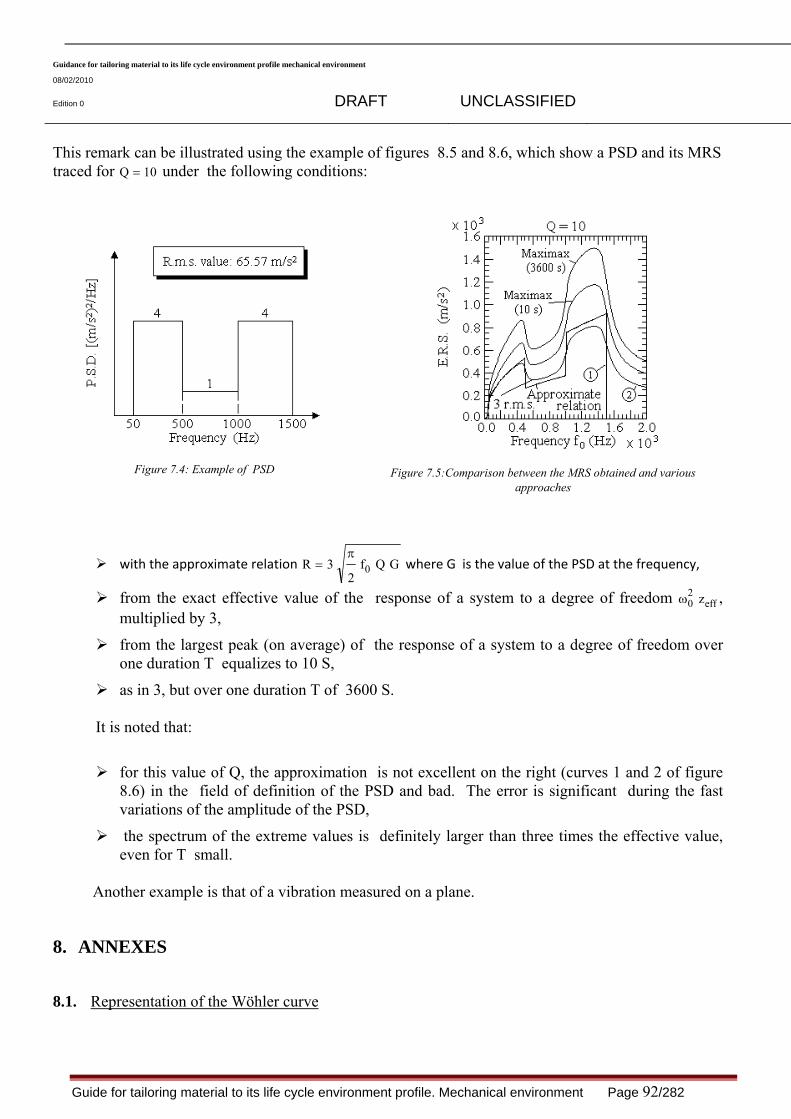
Guidance for tailoring material to its life cycle environment profile mechanical environment
08/02/2010
Edition 0 DRAFT UNCLASSIFIED
Guide for tailoring material to its life cycle environment profile. Mechanical environment Page 92/282
This remark can be illustrated using the example of figures 8.5 and 8.6, which show a PSD and its MRS traced for Q = 10 under the following conditions:
Figure 7.4: Example of PSD
Figure 7.5:Comparison between the MRS obtained and various approaches
with the approximate relation R f Q G= 32
0π
where G is the value of the PSD at the frequency,
from the exact effective value of the response of a system to a degree of freedom ω02 zeff ,
multiplied by 3,
from the largest peak (on average) of the response of a system to a degree of freedom over one duration T equalizes to 10 S,
as in 3, but over one duration T of 3600 S. It is noted that:
for this value of Q, the approximation is not excellent on the right (curves 1 and 2 of figure 8.6) in the field of definition of the PSD and bad. The error is significant during the fast variations of the amplitude of the PSD,
the spectrum of the extreme values is definitely larger than three times the effective value, even for T small.
Another example is that of a vibration measured on a plane.
8. ANNEXES
8.1. Representation of the Wöhler curve

Guidance for tailoring material to its life cycle environment profile mechanical environment
08/02/2010
Edition 0 DRAFT UNCLASSIFIED
Guide for tailoring material to its life cycle environment profile. Mechanical environment Page 93/282
One recalls here after elements on the Wöhler curve and his representation.
8.1.1. WÖHLER Curve : fatigue tests with imposed constraint
If one subjects a test-sample to periodic cycles in traction and compression in imposed constraint of constant amplitude 2
σΔ=S and of null average at constant frequency, one observes a rupture with N
cycles. By repeating this test for various values of S, one obtains a whole of points (N, S), which represented in the plan (N, S), gives a curve called resistance curve (or endurance) to the fatigue or WÖHLER curve (cf figure 8.2).
On this curve, one can distinguish three zones: zone of a plastic or oligocyclic fatigue located in the zone of high amplitude of constraint: the
rupture intervenes after a small number of cycles and is preceded by a notable plastic deformation,
Limite d’endurance
oligocyclique
N
S
N
S forte
Figure 8.1: WÖHLER curve

Guidance for tailoring material to its life cycle environment profile mechanical environment
08/02/2010
Edition 0 DRAFT UNCLASSIFIED
Guide for tailoring material to its life cycle environment profile. Mechanical environment Page 94/282
a zone of fatigue or limited endurance where the rupture is reached after a limited number of
cycles, number which grows when the amplitude of constraint decrease, a zone of unlimited endurance or security zone, under low amplitude of constraint, for which the
rupture does not occur before a high number of cycles, about 710 (or more). In the case of metals, this part of the curve can be approximated by a horizontal asymptote of
which the definite asymptotic value limit of endurance of material in fatigue Dσ .
Let us note that because of the statistical dispersion of the results, the analytical modeling of the WÖHLER curve is often carried out for the average curve.
8.1.2. Analytical modeling of the WÖHLER curve
Several researchers tried to express in the form of equation the WÖHLER curve , i.e. to give an analytical expression providing the number of cycles to the rupture NR according to the amplitude of pressure applied S. They let their names attached to the corresponding laws. One can quote the laws of table 8.1:
Each law makes a better correction of the transition curve modeling between the zone of limited fatigue and the zone of unlimited fatigue, until the law of BASTENAIRE which gets the most realistic representation of the curve of WÖHLER.
Law Analytical expression Remarks
Law of WÖHLER bSaNLn −=
Law of BASQUIN SbLnaNLn −=
Law of STROYMEYER ( )DSbLnaNLn σ−−= These three last laws make it possible to
take into account the limit of endurance of the material σD.
BASTENAIRE allows a probabilistic approach of the curve of WÖHLER.
Law of PALMGREN ( ) ( )DSbLnaBNLn σ−−=+
Law of BASTENAIRE ( )
( )DSc
D
eS
AN σ−−
σ−=
Table8 -1: Analytical expressions of the principal laws

Guidance for tailoring material to its life cycle environment profile mechanical environment
08/02/2010
Edition 0 DRAFT UNCLASSIFIED
Guide for tailoring material to its life cycle environment profile. Mechanical environment Page 95/282
Nevertheless, the BASQUIN law is currently the principal law of acceleration in force in the phase of tests specification because at this stage one cannot characterize the inflections of the Wöhler curve (for example stress limit in the case of steel or the oligocyclic limit in a more general way). This approach is thus conservative because it amounts supposing that all the levels of loading contribute their share to the damage by fatigue, which would not be the case for the levels lower than a possible stress limit.
The danger of this simplification can appear during a reduction of duration, if the constraints produced by the vibrations of the real environment would be lower than the stress limit (infinite lifespan) and where the reduction of the duration of test would lead to constraints under test higher than this limit, with a risk of rupture.
To take account of this difficulty, one could a priori plan to use a representation of the curve of Wöhler defined by two line segments (law Bi-slope), and characterized by two values of the parameter B.
This modification is confronted to the following difficulties [BAR 06]: axis OY of the Wöhler curve gives the constraint which corresponds to the rupture for a number
of given cycles. The FDS is traced starting from the relative displacement of the 1 DDL system, the relation displacement relative vs. constraint not being in general known at the stage of the specifications writing . It is thus not possible to know the ordinate of the change of incline (in relative displacement) of the Wöhler curve ,
the limit stress, clear for steels, does not exist for many materials, the Wöhler curves are very often badly known for the very great numbers of cycles, certain current work highlight the existence of a double inflection (concerning the great numbers
of cycles resulting from a double mechanism at the origin from the ruptures. Between the two strongest slopes, the results are very dispersed, but seem to show a zone close to horizontal. These phenomena are badly known and few data would be available if one wished to hold account of it,
the use of a Bi-slope law in the general case of a structure made up of several materials can lead to a qualification in fatigue insufficient or even erroneous if the most critical component is badly identified.
In the actual position of knowledge, it is preferable to use the Basquin law , even if it can sometimes be conservative.
Note: The experimental validation of the absence of risk of fretting fatigue cannot intervene as long as the definition of the material is not sufficiently advanced. When it is the case, the question is to know if the device concerned with this risk is on the way of a technical function or a function of service. In the first case, the validation falls on the industrialist in charge of the development and is part of the development actions. In the second case, the action should be integrated within the framework of the qualification test of the product. The first case is most frequent and explains why one often does not meet in qualification of the tests dedicated to the control of the risk of fretting corrosion. However, it happens that during endurance tests in qualification are revealed in an unforeseen way of the defects of fretting fatigue. They will have of course to be then corrected. The endurance test in vibration being based on an equivalence of damage being based on the Basquin model with cumulative damage based on Miner Rule does not make it possible to think that this equivalence is also valid for the fretting fatigue. It is thus the effect of a lucky chance which allowed this revelation.

Guidance for tailoring material to its life cycle environment profile mechanical environment
08/02/2010
Edition 0 DRAFT UNCLASSIFIED
Guide for tailoring material to its life cycle environment profile. Mechanical environment Page 96/282
8.2. guarantee Coefficient and test factor : abacuses

Guidance for tailoring material to its life cycle environment profile mechanical environment
08/02/2010
Edition 0 DRAFT UNCLASSIFIED
Guide for tailoring material to its life cycle environment profile. Mechanical environment Page 97/282
Abacus N° 1-a

Guidance for tailoring material to its life cycle environment profile mechanical environment
08/02/2010
Edition 0 DRAFT UNCLASSIFIED
Guide for tailoring material to its life cycle environment profile. Mechanical environment Page 98/282
Abacus N° 1-b

Guidance for tailoring material to its life cycle environment profile mechanical environment
08/02/2010
Edition 0 DRAFT UNCLASSIFIED
Guide for tailoring material to its life cycle environment profile. Mechanical environment Page 99/282
Abacus N° 1-c

Guidance for tailoring material to its life cycle environment profile mechanical environment
08/02/2010
Edition 0 DRAFT UNCLASSIFIED
Guide for tailoring material to its life cycle environment profile. Mechanical environment Page 100/282
Abacus N° 1-d

Guidance for tailoring material to its life cycle environment profile mechanical environment
08/02/2010
Edition 0 DRAFT UNCLASSIFIED
Guide for tailoring material to its life cycle environment profile. Mechanical environment Page 101/282
Abacus N° 2-a

Guidance for tailoring material to its life cycle environment profile mechanical environment
08/02/2010
Edition 0 DRAFT UNCLASSIFIED
Guide for tailoring material to its life cycle environment profile. Mechanical environment Page 102/282
Abacus N° 2-b

Guidance for tailoring material to its life cycle environment profile mechanical environment
08/02/2010
Edition 0 DRAFT UNCLASSIFIED
Guide for tailoring material to its life cycle environment profile. Mechanical environment Page 103/282
Abacus N° 2-c

Guidance for tailoring material to its life cycle environment profile mechanical environment
08/02/2010
Edition 0 DRAFT UNCLASSIFIED
Guide for tailoring material to its life cycle environment profile. Mechanical environment Page 104/282
Abacus N° 2-d

Guidance for tailoring material to its life cycle environment profile mechanical environment
08/02/2010
Edition 0 DRAFT UNCLASSIFIED
Guide for tailoring material to its life cycle environment profile. Mechanical environment Page 105/282
Abacus N° 3-a

Guidance for tailoring material to its life cycle environment profile mechanical environment
08/02/2010
Edition 0 DRAFT UNCLASSIFIED
Guide for tailoring material to its life cycle environment profile. Mechanical environment Page 106/282
Abacus N° 3-b

Guidance for tailoring material to its life cycle environment profile mechanical environment
08/02/2010
Edition 0 DRAFT UNCLASSIFIED
Guide for tailoring material to its life cycle environment profile. Mechanical environment Page 107/282
Abacus N° 3-c

Guidance for tailoring material to its life cycle environment profile mechanical environment
08/02/2010
Edition 0 DRAFT UNCLASSIFIED
Guide for tailoring material to its life cycle environment profile. Mechanical environment Page 108/282
Abacus N° 3-d

Guidance for tailoring material to its life cycle environment profile mechanical environment
08/02/2010
Edition 0 DRAFT UNCLASSIFIED
Guide for tailoring material to its life cycle environment profile. Mechanical environment Page 109/282
Abacus N° 4-a
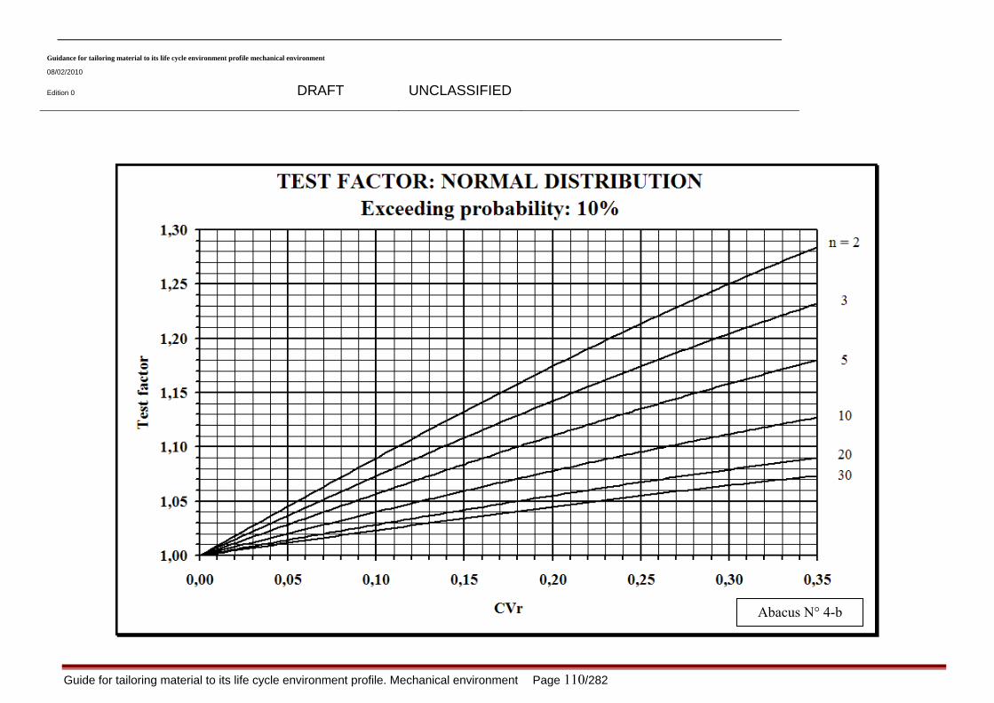
Guidance for tailoring material to its life cycle environment profile mechanical environment
08/02/2010
Edition 0 DRAFT UNCLASSIFIED
Guide for tailoring material to its life cycle environment profile. Mechanical environment Page 110/282
Abacus N° 4-b

Guidance for tailoring material to its life cycle environment profile mechanical environment
08/02/2010
Edition 0 DRAFT UNCLASSIFIED
Guide for tailoring material to its life cycle environment profile. Mechanical environment Page 111/282
Abacus N° 4-c

Guidance for tailoring material to its life cycle environment profile mechanical environment
08/02/2010
Edition 0 DRAFT UNCLASSIFIED
Guide for tailoring material to its life cycle environment profile. Mechanical environment Page 112/282
Abacus N° 5-a

Guidance for tailoring material to its life cycle environment profile mechanical environment
08/02/2010
Edition 0 DRAFT UNCLASSIFIED
Guide for tailoring material to its life cycle environment profile. Mechanical environment Page 113/282
Abacus N° 5-b

Guidance for tailoring material to its life cycle environment profile mechanical environment
08/02/2010
Edition 0 DRAFT UNCLASSIFIED
Guide for tailoring material to its life cycle environment profile. Mechanical environment Page 114/282
Abacus N° 5-c

Guidance for tailoring material to its life cycle environment profile mechanical environment
08/02/2010
Edition 0 DRAFT UNCLASSIFIED
Guide for tailoring material to its life cycle environment profile. Mechanical environment Page 115/282
Abacus N° 6-a

Guidance for tailoring material to its life cycle environment profile mechanical environment
08/02/2010
Edition 0 DRAFT UNCLASSIFIED
Guide for tailoring material to its life cycle environment profile. Mechanical environment Page 116/282
Abacus N° 6-b

Guidance for tailoring material to its life cycle environment profile mechanical environment
08/02/2010
Edition 0 DRAFT UNCLASSIFIED
Guide for tailoring material to its life cycle environment profile. Mechanical environment Page 117/282
Abacus N° 6-c

Guidance for tailoring material to its lifcycle environment profile mechanical environment
08/02/2010 Edition 0 DRAFT UNCLASSIFIED
Guide d’application de la démarche de prise en compte de l’environnement mécanique Page 118/282
8.3. Calculation of the MRS The MRS of a vibration can be calculated: That is to say directly starting from a sample of signal of time. It gives then, at each Eigen
frequency, the value of the largest peak of the response of a system to 1 ddl observed for this sample. So that the result is statistically satisfactory, it is necessary thus that the sample has one sufficient duration. No assumption is here necessary on the nature of the signal (random stationary or not...). The research of the peak greatest east carried out starting from the numerical calculation of the answer,
That is to say, if the signal is stationary Gaussian, starting from his PSD. One then obtains at each eigen frequency the value of the largest peak, on average, over the duration T chosen for calculation. (je pense qu’on peut ôter les of)
The process is as follows [ LAL 94 ] [ LAL 02c ] [ LAL 02d ]: calculation of the PSD of the vibratory signal, calculation of the effective values of displacements, speed and acceleration relating of the response of the system to a degree of freedom starting from the PSD,
calculation of the average frequency and the average number of peaks per unit of time, calculation of the coefficient of irregularity R of the answer, determination of the density of probability of the peaks of the answer,
⎥⎥⎥
⎦
⎤
⎢⎢⎢
⎣
⎡
⎟⎟⎟
⎠
⎞
⎜⎜⎜
⎝
⎛
−++
π
−=
−−
−
)r1(2
ruerf1e
2ru
e2
r1)u(q
22
u)r1(2
u2
2
2
2
[8.1]
Determination the function distribution of the peaks of the answer.
( ) ( )( ) ( )
20u
0 020 02 2
u r u1Q u 1 P u 1 erf r e 1 erf2 2 1 r 2 1 r
−⎧ ⎫⎡ ⎤⎛ ⎞ ⎛ ⎞⎪ ⎪⎢ ⎥⎜ ⎟ ⎜ ⎟⎪ ⎪⎢ ⎥⎜ ⎟ ⎜ ⎟= − = − + +⎨ ⎬⎢ ⎥⎜ ⎟ ⎜ ⎟⎪ ⎪− −⎜ ⎟ ⎜ ⎟⎢ ⎥⎪ ⎪⎝ ⎠ ⎝ ⎠⎣ ⎦⎩ ⎭
[8.2]
where ( )Q u0 is the probability that u u> 0 The method consists in setting a value of ( )Q u0 and seeking the value of u0 corresponding. The average total number of peaks higher than u0 over one duration T is equal to
( )N n T Q up= +0 [8.3]
The largest peak during T (on average) corresponds roughly to the level u0 which is exceeded only once, from where

Guidance for tailoring material to its life cycle environment profile mechanical environment
08/02/2010
Edition 0 DRAFT UNCLASSIFIED
Guide for tailoring material to its life cycle environment profile. Mechanical environment Page 119/282
( )Q un Tp
01
= + [8.4]
The level u0 is determined by successive iterations. The function of distribution ( )Q u being a
decreasing function of u, one gives itself two values of u such as:
( ) ( ) ( )Q u Q u Q u1 0 2< < [8.5]
and, to each iteration, one reduces the interval (u1, u2) until, for example, ( ) ( )
( )Q u Q u
Q u1 2
0
210−
< −
From where, by interpolation,
( ) ( ) ( )( ) ( )
z z z u uQ u Q u
Q u Q uus eff≈ = −
−
−+
⎡
⎣
⎢⎢
⎤
⎦
⎥⎥0 2 1
1 0
1 21 [8.6]
and
( ) ( ) ( ) ( ) ( )( ) ( )
R f z f z u uQ u Q u
Q u Q uus eff= ≈ −
−
−+
⎡
⎣
⎢⎢
⎤
⎦
⎥⎥
2 202
02
2 11 0
1 21π π [8.7]
In this last case, the most precise method of calculation of the MRS uses the distribution of maximum [LAL 94] [LAL 09c] :
( ) ( )( ) ( )
20u
0 020 02 2
u r u1Q u 1 P u 1 erf r e 1 erf2 2 1 r 2 1 r
−⎧ ⎫⎡ ⎤⎛ ⎞ ⎛ ⎞⎪ ⎪⎢ ⎥⎜ ⎟ ⎜ ⎟⎪ ⎪⎢ ⎥⎜ ⎟ ⎜ ⎟= − = − + +⎨ ⎬⎢ ⎥⎜ ⎟ ⎜ ⎟⎪ ⎪− −⎜ ⎟ ⎜ ⎟⎢ ⎥⎪ ⎪⎝ ⎠ ⎝ ⎠⎣ ⎦⎩ ⎭
[8.8]
where ( )Q u0 is the probability that u u> 0 The method consists in setting a value of ( )Q u0 and seeking the value of u0 corresponding. The average total number of peaks higher than u0 over one duration T is equal to
( )N n T Q up= +0 [8.3]
The largest peak during T (on average) corresponds roughly to the level which is exceeded only
once, from where
( )Q un Tp
01
= + [8.9]
The level is determined by successive iterations. The function of distribution being a decreasing function of U, one gives itself two values of U such as:

Guidance for tailoring material to its life cycle environment profile mechanical environment
08/02/2010
Edition 0 DRAFT UNCLASSIFIED
Guide for tailoring material to its life cycle environment profile. Mechanical environment Page 120/282
( ) ( ) ( )Q u Q u Q u1 0 2< <
and, to each iteration, one reduces the interval (u1, u2) until, for example,
[8.10]
( ) ( )( )
Q u Q u
Q u1 2
0
210−
< −
From where, by interpolation,
( ) ( ) ( )( ) ( )
z z z u uQ u Q u
Q u Q uus eff≈ = −
−
−+
⎡
⎣
⎢⎢
⎤
⎦
⎥⎥0 2 1
1 0
1 21 [8.11]
And
( ) ( ) ( ) ( ) ( )( ) ( )
R f z f z u uQ u Q u
Q u Q uus eff= ≈ −
−
−+
⎡
⎣
⎢⎢
⎤
⎦
⎥⎥
2 202
02
2 11 0
1 21π π
[8.12]
Example:
Random vibration defined by:
100 - 300 Hz...........5 (ms-2)2/Hz 300 - 600 Hz.........10 (ms-2)2/Hz 600 - 1 000 Hz...........2 (ms-2)2/Hz

Guidance for tailoring material to its life cycle environment profile mechanical environment
08/02/2010
Edition 0 DRAFT UNCLASSIFIED
Guide for tailoring material to its life cycle environment profile. Mechanical environment Page 121/282
Duration: 1 hour
The extreme spectrum of answer is traced on figure 8.2 for 5 15000≤ ≤f Hz and Q = 10 .
Figure 8.2 MRS of a random vibration defined by its PSD:
Note: The MRS can also be calculated starting from simplifying assumptions:
calculation of the MRS to leave the instantaneous values of the answer,
The reasoning is based on the assumption that the studied vibration is Gaussian with null average. The distribution of the instantaneous values of the answer is then itself Gaussian and, if and are independent functions, the average number a second passages of a level has with positive slope can be written :
n n ea
a
zeff+ +−
= 02
2
2
[8.13]
Maybe, over one duration T:
N n T ea
a
zeff+ +−
= 02
2
2
[8.14]
The largest level for this length of time T is that which is exceeded only once:
N n T ea
a
zeff+ +−
= =1 02
2
2
[8.15]
From where the level has
a z n Teff= +2 0ln [8.16]

Guidance for tailoring material to its life cycle environment profile mechanical environment
08/02/2010
Edition 0 DRAFT UNCLASSIFIED
Guide for tailoring material to its life cycle environment profile. Mechanical environment Page 122/282
With the frequency considered (and for the selected value of Q), the extreme spectrum of answer has as an amplitude:
( )R f a= 2 02
π
( )R f z n Teff= +2 202
0π ln [8.17] The probability so that this level is reached in a time lower or equal to T is given by:
( )P T ee
n
na
a= − = − =−
+
+
1 11
0 632,
The MRS could be given for a probability P 0 data of going beyond of the threshold has starting
from the relation:
( ) ( ) ( ){ }20 eff 0 0R 2 f z 2 ln n T ln ln 1 P+= π − − −⎡ ⎤⎣ ⎦ [8.18]
Limit of the MRS at the great frequencies

Guidance for tailoring material to its life cycle environment profile mechanical environment
08/02/2010
Edition 0 DRAFT UNCLASSIFIED
Guide for tailoring material to its life cycle environment profile. Mechanical environment Page 123/282
When the Eigen frequency becomes large compared to the upper limit of the field of definition of the entered PSD, the average frequency of relative displacement answer tends towards that of the excitation. It is then independent of the Eigen frequency of the excited system. The expression [ 8.22 ] of the MRS thus has as a limit:
20 sup eff mxz x 2 ln f Tω ≈ &&&& [8.19]
effx&& = effective value of the analyzed signal
mxf && = average frequency of the vibratory signal T = duration of the vibration One finds the general property of the spectra of response to the shock which tend high frequency towards the largest value of the excitation.
MRS calculated starting from the distribution of the largest peaks of the answer,
On the assumption of a response to narrow band and a law of distribution of the peaks of the response of Rayleigh, it is possible to determine the law of distribution of the peaks and to calculate of it average [ LAL 02c ].
0n T2
iuP(u u) 1 exp2
+
⎡ ⎤⎛ ⎞< = − −⎢ ⎥⎜ ⎟⎜ ⎟⎢ ⎥⎝ ⎠⎣ ⎦
[8.20]
One deduces the expression from it from the MRS:
( )220 sup 0 eff 0
0
z 2 f z 2 ln n T2 ln n T
+
+
⎡ ⎤ε⎢ ⎥ω = π +⎢ ⎥⎣ ⎦
[8.21]
It should be noted that the expression [ 3.2 ] above is an approximation of this result for 0n T+ large.
spectrum of answer defined by k time the effective answer.
The assumption is made that the distribution of the instantaneous values of the answer is Gaussian. Each point of the spectrum represents the answer which has a constant probability fixed not to be exceeded.

Guidance for tailoring material to its life cycle environment profile mechanical environment
08/02/2010
Edition 0 DRAFT UNCLASSIFIED
Guide for tailoring material to its life cycle environment profile. Mechanical environment Page 124/282
Figure 8.3: Decomposition of the PSD in segments for the calculation of effective displacement
The MRS is obtained by drawing the graph of the following function :
( )R k f zeff= 2 02
π [8.22]
according to f0, forξ given [BAN 78]. Constant K is selected so as to be able to affirm, with a given probability P0 , that the maximum of the response is lower, at a frequency f0, than the ordinate of spectrum [BAD 70]. Probability P0 is maintained constant whatever f0.
Being given a PSD calculated starting from an acceleration ( )&&x t (cf figure 8.3), the effective value of response displacement zeff of a linear one degree of freedom system , having frequency f0 and of given dampingξ, is extracted from [LAL 09d],
( )z
fa Geff j j
j
n2
403
14 2=
=
∑π
ξ π [8.23]
or, if the PSD is represented with horizontal segments, by:
i 1
i
h2ni2
eff 3 2i 1 0 h
G h h 1 2 h 2 hz ln Arc tan Arc tan
2 24 h h 1
+
=
⎡ ⎤+ α + +α −αξ⎢ ⎥= + +⎢ ⎥α ξ ξξ ω −α +⎣ ⎦
∑ [8.24]
The effective response can be given in a more approximate way using the relation [BAN 78]
[FOS 82] [SHO 68] :
( )ωπ
02
02
z f Q G feff x= && [8.25]
Established with assumption that Gx&& is a white noise, by considering that, if Gx&& is unspecified, the response is mainly due to the values of the PSD at the frequencies located around resonance.
If the PSD varies little around 0f , this relation gives an approximate value of zeff acceptable even for a formed noise. The value k = 3 is often retained for the estimate of the extreme peaks; K. Foster

Guidance for tailoring material to its life cycle environment profile mechanical environment
08/02/2010
Edition 0 DRAFT UNCLASSIFIED
Guide for tailoring material to its life cycle environment profile. Mechanical environment Page 125/282
chooses k = 2 2, for the studies of rupture by fatigue [FOS 82]. The choice of a constant value K is often criticized, because there is no reason to consider a particular value 3,4 or 5, a large occasional peak being able to start a crack which will be propagated then with the smaller constraints [BHA 58] [GUR
82] [LEE 82] [LUH 82]. The MRS ω02 zeff is also some times defined for k = 1.
The MRS is calculated: either in an exact way starting from the effective value of the PSD response determined with the
transfer function [STA 76], or starting from the approximate relation [8.25] [SCH 81]. One chooses first of all Q factor
according to the experience gained on the concerned material (5 to 15 in general) or, more generally, one retains the conventional value Q = 10.
Each point of the PSD is used to evaluate ω0
2 zeff using
R k f Q Gi i i=π
20 [8.26]
while proceeding as indicated on figure 8.4 (calculation of Ri at each frequency to pass from the PSD to the MRS).
Figure 8.4: Simplified calculation of the MRS starting from a PSD
Limit of the approximate methods for calculation of the extreme answers:
Precision obtained starting from the expression R f Q Gi i= 32
0π
is of as much better than Q
factor is larger. The precision is also function of the position of f i0 compared to the terminals f1 and f2 PSD.
This remark can be illustrated using the example of figures 8.5 and 8.6, which show a PSD and its
MRS traced for Q = 10 under the following conditions:

Guidance for tailoring material to its life cycle environment profile mechanical environment
08/02/2010
Edition 0 DRAFT UNCLASSIFIED
Guide for tailoring material to its life cycle environment profile. Mechanical environment Page 126/282
Figure 8.5: Example of PSD
Figure 8.6: Comparison between the MRS obtained by various approaches
with the approximate relation R f Q G= 32
0π
where G is the value of the PSD at the
frequency f f= 0,
from the exact effective value of the response of a system to a one degree of freedom ω02 zeff ,
multiplied by 3,
starting from the largest peak (on average) of the response of a system to a degree of freedom over one duration T equalizes to 10 S,
as in 3, but over one duration T of 3600 S.
It is noted that:
for this value of Q, the approximation is not excellent on the right (curves 1 and 2 of figure 8.6) in the field of definition of the PSD and bad. The error is important during the fast variations of the amplitude of the PSD,
the spectrum of the extreme values is definitely larger than three times the effective value, even for T small.
Another example is that of a vibration measured on a plane.

Guidance for tailoring material to its life cycle environment profile mechanical environment
08/02/2010
Edition 0 DRAFT UNCLASSIFIED
Guide for tailoring material to its life cycle environment profile. Mechanical environment Page 127/282
Figure 8.7: Example of a PSD vibration measured on a plane
The MRS are calculated starting from the PSD of this environment (cf figure 8.7) for Q = 50 (cf figure 8.8) and for Q = 5 (cf figure 8.9):
with the approximate relation32
0π
f Q G ,
with 3 0
2ω zeff (zeff being the exact effective value),
with the largest peak for one duration T = 1 hour.
Figure 8.8: MRS of a vibration measured on a plane (Q=50)
Figure 8.9: MRS of a vibration measured on a plane (Q=5)
It is noted that for:

Guidance for tailoring material to its life cycle environment profile mechanical environment
08/02/2010
Edition 0 DRAFT UNCLASSIFIED
Guide for tailoring material to its life cycle environment profile. Mechanical environment Page 128/282
Q = 50, the approximation is good, the spectra with 3 02ω zeff being in addition much lower
than the curve giving the largest peak, Q = 5, the three spectra are appreciably different.
8.4. Historical background
Until beginning of the years 80, the environment specifications were extracted from normative documents which proposed standard tests severities which were very enveloping of the real conditions of use values actually recorded .
The values suggested in these documents were in general given starting from measurements. The transformation of these measurements into specifications was the subject of several methods, the most used being that by envelope of the power spectral density (PSD). It consists in calculating the PSD of several measurements taken in several points and/or under various conditions, then to trace their envelope. This method, simple in its principle, is however very sensitive to the way in which the envelope is simplified to transform it into specification. The transformation real environment/specification is based on the reproduction of the contents in frequency of the real vibrations and not on an equivalence of the mechanical effects of the vibrations. In its initial version, it does not take account of the differences of the durations of the vibrations which one calculates the PSD envelope (there exists a more elaborate method derived which makes it possible to mitigate this gap [LAL 09e] using the rule of reduction of duration resulting from the law of Basquin, but it is used very little). So it can result in applying to the material under test over one long life of the vibratory levels relative to a certain beach of frequencies which are present only during one short duration in the real environment.
All these standards provide lists of values among which the user must choose those to include in his schedule of conditions.
In the years 1980/1986, standards GAM EG13 [GAM 86] (evolution of French standard GAM T13) and MIL STD 810D (in the United States) underwent a deep modification of their philosophy while asking the specificator to use measurements of the real environment to write the specifications (tailoring of the tests). It is a completely new approach in the standards, which requires to analyze the condition of uses, to associate measurements with each type of foreseeable environment and to synthesize all these values to transform them into specifications of reasonable duration.
These stages all are important. Most technical is that which results in seeking a vibration of the same severity than all those of the profile of life (or of a part). The methods are a priori those already described hereabove.
8.5. Measurements validation
Let us recall that the second part of the mechanical general appendix OF game g 13 entitled “signal Treatment ” is precisely intended to bring a didactic support in signal treatment at the time of the various steps of implementation of the criteria and tools for validation.
The various chapters of this document describe :

Guidance for tailoring material to its life cycle environment profile mechanical environment
08/02/2010
Edition 0 DRAFT UNCLASSIFIED
Guide for tailoring material to its life cycle environment profile. Mechanical environment Page 129/282
the signal sampling, the periodic signals, the random signals, an additional referring to:
o the classification of the signals, o Fourier series and transforms , o convolution, o type of windows and associated functions, o Dirac transforms , o Hilbert transform, o Elements of statistic, o Errors on random functions.
In the validation analysis , one could distinguish between the criteria having a general character and those being specific:
8.5.1. general Criteria
8.5.1.1. zero drifts
One distinguishes two types of drift of zero: permanent and constant offset, including before the beginning of appearance of the physical
phenomenon if this one appears in the course of measurement, Static Offset : shift compared to the zero of the median value of the signal before the beginning of the physical phenomenon.
drift started at one unspecified moment to the measure, with an unspecified temporal evolution on whole or part of the signal, Dynamic offset (DOF): evolution of the median value of the signal following the appearance of the physical phenomenon in general it is accompanied by a drift speed, speed obtained by integration of acceleration. Its characterization by only one value would suppose to fix the terminals of integration.
8.5.1.2.Saturation
No saturation is tolerated as its correction is not possible. Fear of saturating often led the teams to size the effective ranges in way too much broad, and hence
to degrade quantification noise. It is worth however sometimes to have a slightly saturated signal. To have a calculation PSD or MRS result notably different requires a signal is strongly saturated.
8.5.1.3.The quantification resolution QR
Expressed by the relationship between the resolution in acceleration brought back to the
difference between the maximum value and the minimal value measured max min
Δa a a
QR =− .
8.5.1.4.Signal to Noise ratio (SNR)
Difference between the SRS of the noise recorded before the beginning of measurement, (called noise of reference) and that of the part of the signal which starts 1 ms before the detection of the

Guidance for tailoring material to its life cycle environment profile mechanical environment
08/02/2010
Edition 0 DRAFT UNCLASSIFIED
Guide for tailoring material to its life cycle environment profile. Mechanical environment Page 130/282
appearance of the physical phenomenon and which at the same duration as the noise of reference (20 ms for example).
8.5.1.5.Dissymmetry of the signal(RSd.)
Case of a vibration: variation between the MRS of the positive part of the signal and that of its negative part RSd. = |(MRS+) – (MRS-)|
Case of a shock: variation between the SRS of the positive part of the signal and that of its negative part RSd.= |SRS+ - SRS-|
8.5.1.6.Stationnarity
In a strict sense, characterizes the constancy of every central moment during the signal evolution . In the broad sense, one limits the verification of this requirement to the central moments:
of order 2: effective value, of order 3: asymmetry(skewness), of order 4: flatness(kurtosis),
8.5.2. specific Criteria
8.5.2.1.Case of the pyrotechnical shocks
The limits values hereafter are extracted from reference [HDD]
8.5.2.1.1. zero Drifts
This one gives a criterion on speed declined in two alternatives according to the type of shock met: shock with zero net velocity variation : measurement is to be rejected if the median
velocity , calculated over all the duration of the recording, exceeds the extreme values recorded at the time of the temporal transient,
shock with non zero net velocity variation: measurement is to be rejected if the value speed at the end of the recording exceeds of a factor 2 the value of the expected velocity variation.
8.5.2.1.2.quantification resolution
The quantification step QR is defined in the 8.5.1.3 paragraph. The criteria of validation are: QR < 0,5% measurement withhold, 0,5% <PM < 5% measurement withhold with reserve, PM > 5% measurement discarded.
8.5.2.1.3.Signal to Noise ratio
SNR > 6 dB on all the frequency range : measures withhold, SNR < 6 dB on less than 20% of the spectrum measures acceptable with reserve, SNR < 6 dB on more than 20% of the spectrum measures discarded.

Guidance for tailoring material to its life cycle environment profile mechanical environment
08/02/2010
Edition 0 DRAFT UNCLASSIFIED
Guide for tailoring material to its life cycle environment profile. Mechanical environment Page 131/282
8.5.2.1.4. signal to noise ratio
MR. > 6 dB on all the frequency range measures withhold, MR. < 6 dB on less than 20% of the spectrum measures acceptable with reserve, MR. < 6 dB on more than 20% of the spectrum measures discarded.
8.6. Synthesis of the environment without taking into account the FDS
8.6.1. Illustration on a nonstationary signal of the disadvantages of the PSD envelope method :
A real environment is not stationary if its effective value varies in function of time over one more or less large duration (shifting of speed of a road vehicle, turbulences during a flight plane, etc). In such a case, it is not correct to calculate a power spectral density to represent the phenomenon and it is thus not possible to establish a specification by envelope of the PSD.
Example: Figure 8.10 presents a signal obviously nonstationary, which one calculated the total effective value over 5 seconds to give an order of magnitude, knowing that this effective value is not very significant since it varies according to time. Figure 8.11 gives of them the variations, which are very marked.
Figure 8.10: Nonstationary vibration by variation of its effective acceleration in function of time
The duration was limited here to 5 S, but it could be much larger. The calculation of the PSD of such a signal is mathematically possible (cf figure 8.12), although without significance (average of blocks having an effective value different for reasons nonrelated to random nature from the signal).

Guidance for tailoring material to its life cycle environment profile mechanical environment
08/02/2010
Edition 0 DRAFT UNCLASSIFIED
Guide for tailoring material to its life cycle environment profile. Mechanical environment Page 132/282
Figure 8.11: Variation according to the time of the effectiveacceleration of the nonstationary vibration of figure 8.10
Figure 8.12: PSD of the nonstationary vibration of figure 8.10
To show the error made by using this PSD like specification, we compared it with that deduced from a spectrum of fatigue damage calculated directly starting from the signal according to time (cf figure 8.13).

Guidance for tailoring material to its life cycle environment profile mechanical environment
08/02/2010
Edition 0 DRAFT UNCLASSIFIED
Guide for tailoring material to its life cycle environment profile. Mechanical environment Page 133/282
Figure 8.13: Comparison of the PSD of the nonstationary vibration (figure 8.12) and of the PSD established by equivalence
damage starting from the signal according to time (figure 8.10)
The specifications obtained are very different, at the same time with regard to the contents in frequency and the effective value. The consequences of these differences are found on their MRS and FDS (cf figures 8.14 and 8.15).
Figure 8.14: MRS of the PSD of figure 8.13

Guidance for tailoring material to its life cycle environment profile mechanical environment
08/02/2010
Edition 0 DRAFT UNCLASSIFIED
Guide for tailoring material to its life cycle environment profile. Mechanical environment Page 134/282
Figure 815: FDS of the PSD of figure 8.13
The specification which would result from the PSD of the signal underestimates the severity of the vibration clearly whatever the criterion (MRS or FDS).
In the case of the nonstationary vibrations (or not Gaussian), the MRS and FDS must be calculated directly starting from the signal according to time. The specification deduced from this FDS is expressed in the form of a PSD of a Gaussian stationary random vibration (the control shaker softwares can generate to day only vibrations of this type) which produces at each frequency the same damage and the same maximum constraint as the real environment vibration .
8.6.2. Case of a carrying under plane
The tailoring approach described below was carried out within the framework of an international program. The goal is to show an example of construction of specifications of test starting from measurements in flight of carrying, without using the MRS/FDS, but only the PSD with an analysis of the effective values according to the flight parameters .
8.6.2.1. Test plan - flight measurements
One or more test flight with instrumented mock ups are carried out to characterize the environment, and to decline it in terms of test severities . The instrumentation generally covers all the equipments of the model or the interface plane/model. That led to a big number of acceleration measurement inputs (50 to 100 channels of measurement per model for example). These measurements are carried out according to a test programme adapted to characterize the environment (gathering dated); the situations of flight cover the flight domain alternating the phases of stationary flight level and non stationary connecting operations such as barrels, turns with strong load factor, exit of the air-brakes, etc measurements are extracted according to time intervals selected starting from the principal flight parameters , known to be influential according to the carrier aircraft: speed, the Mach number, altitude, the load factor, the incidence, the skid, etc….

Guidance for tailoring material to its life cycle environment profile mechanical environment
08/02/2010
Edition 0 DRAFT UNCLASSIFIED
Guide for tailoring material to its life cycle environment profile. Mechanical environment Page 135/282
The configuration of the plane with the presence or not of close armament is also a parameter to be taken into account in the analysis of measurements. The number of covered flight situations is thus generally higher than 100. From where a number of data of about 10000 (with 100 channels of measurement) for a flight test. These tests thus generate with a very important flood of data requiring to install effective tools for data analysis which employ in our case, internationally adapted and recognized methods to analyze and decline these measurements in terms of specifications in an industrial context.
8.6.2.2.Analyzes measurements
The first step consists in validating and analyzing measurements, according to the flight situations . The anomalies of measurement are inevitable on a great number of ways (problem sensitivity of the sensor, poor contacts, errors on the axis of detection, etc….). An analysis as of the first flight makes it possible to react quickly and to intervene on instrumentation I to correct the errors. The follow-up of the levels of acceleration according to the flight parameters makes it possible to check coherence and to extract some rules making it possible to extrapolate with a good confidence the levels in the flight domain , when the tests do not cover all the field.
8.6.2.3.Dynamic pressure - effective value
For an airborne material in external load, the captive flight is characterized by several sources of excitation:
structural excitations being transmitted by the points of interface with the carrier, aerodynamic origin excitation.
In the phases of stationary flight levels, the aerodynamic excitation proves to be the predominent source of excitation. It takes the top compared to the excitation whose frequential characteristics are such, that the first modes of structure are slightly excited. A contrario, the structural modes can be strongly excited in the case of certain non stationary phase (manoeuvres, buffeting). So that an important parameter governing the ambient vibrations is the dynamic pressure. The approach is based on the analysis of the effective temporal measured signal according to the dynamic pressure. Several flight campaigns on various carriers and materials showed that the law of evolution recommended by the Anglo-Saxon standards (a line in scale log-log) is well checked, in particular when the point of carrying is located under the fuselage and as illustrated of figure 8.16.

Guidance for tailoring material to its life cycle environment profile mechanical environment
08/02/2010
Edition 0 DRAFT UNCLASSIFIED
Guide for tailoring material to its life cycle environment profile. Mechanical environment Page 136/282
Valeur efficace en fonction de la pression dynamique
0,1
1
10
10 100 1000Pression dynamique (hpa)
Grm
s
Figure 8.16: Effectiveacceleraion evolution VS. dynamic pressure
If λ is the slope of the line, one has for two points of flight 1 and 2 λ
⎟⎟⎠
⎞⎜⎜⎝
⎛=
2
1
2
1
pp
gg
where gi and pi are respectively the effective acceleration and the dynamic pressure of the point of flight 1.
This law is used: to extrapolate if necessary, in a conservative way by taking the effective λ raising, values
starting from the measured points of flight and to cover all the flight envelope, to characterize all the points of flight in terms of PSD, (cf chapter 4), to take into account in the development of severities of test tiredness equivalent to a
profile of life given: not discussed in chapter 5. The approach is this conservative time by taking λ undervaluing.
8.6.2.4.Frequential contents
In the same way the frequential contents and its evolution according to the flight parameters are
analyzed. The PSD are calculated, by flight situation , with a frequential resolution ranging between 1 and 2 Hz. The environment with its frequential contents is modelled according to the dynamic pressure, for each input of measurement, by building a homothetic profile which frames the envelope of the measured PSD for a dynamic range of given pressure. The effective acceleration of this profile, by dynamic range of
pressure, follows the law then λ
⎟⎟⎠
⎞⎜⎜⎝
⎛=
2
1
2
1
pp
gg
: to see the example given figure 32.
One obtains in terms of PSD: λ2
2
1
2
1⎟⎟⎠
⎞⎜⎜⎝
⎛=
pp
dspdsp , where PSDi, and pi are respectively the power
specral density and the dynamic pressure of the point of flight 1.

Guidance for tailoring material to its life cycle environment profile mechanical environment
08/02/2010
Edition 0 DRAFT UNCLASSIFIED
Guide for tailoring material to its life cycle environment profile. Mechanical environment Page 137/282
This approach can be carried out by gathering certain phases of flight, for example in two categories: stationary phases and non stationary phases. Finally a coefficient is applied to the envelopes of PSD to take into account dispersions related on measurements and the materials.
Evolution DSP en fonction de la pression dynamique
0,000001
0,00001
0,0001
0,001
0,01
1 10 100 1000 10000Fréquence (Hz)
DSP
(g²/H
z) 100 hpa
300 hpa
700 hpa500 hpa
Evolution DSP en fonction de la pression dynamique
0,000001
0,00001
0,0001
0,001
0,01
1 10 100 1000 10000Fréquence (Hz)
DSP
(g²/H
z) 100 hpa
300 hpa
700 hpa500 hpa
Figure 8.17: Dynamic evolution PSD/pressure
8.6.2.5.Duration of tests to cover the life profile
To specify an equivalent test severity in terms of fatigue damage, without using the FDS, the flight profiles of the material carried under plane are splitted by dynamic values of pressure. That led to a histogram given on figure 8.18.
The distribution of the durations on the one hand, and the relations between the effective values and the dynamic pressure on the other hand, make it possible to reduce each duration relative to a range of dynamic pressure, by increasing its level up to the highest level corresponding to the maximum dynamic pressure. The law of Basquin is used.
Total duration ∑i
itof flight is equivalent in term of fatigue damage, at one duration of test of:
∑=
⎟⎟⎠
⎞⎜⎜⎝
⎛=
n
ii
b
n
ieéquivalent t
ggt
1 , with in addition
λ
⎟⎟⎠
⎞⎜⎜⎝
⎛=
n
i
n
i
pp
gg
N being the number of dynamic section of pressure.
The Anglo-Saxon standards recommend a parameter Bof 5 (from where denomination “fifth power law”)
The level of test, applied for one equivalent length of time T, is defined with a gauge in PSD wrapping all the situations, raised of a coefficient to free itself from dispersions. This approach, not using the MRS/FDS, conduit at contracted durations of test, being able to reach for example 10 hours equivalent to 100 hours because the plane always does not fly to full airspeed indicator.

Guidance for tailoring material to its life cycle environment profile mechanical environment
08/02/2010
Edition 0 DRAFT UNCLASSIFIED
Guide for tailoring material to its life cycle environment profile. Mechanical environment Page 138/282
Durée d'emport par tranche de pression dynamique
0%
5%
10%
15%
20%
25%
30%
100 200 300 400 500 600 700
Presion dynamique (hpa)
Figure 8.18: Histogram - flight profiles
8.6.2.6.Advantages and limits
This approach has the advantage of being rather simple to deploy to treat important volumes of data. It also makes it possible to easily compare two profiles of flight different in terms of fatigue damage.
This approach leads to a result theoretically identical to an FDS approach, provided that the power law is checked. I.e. figures 1 and 2 accurately represent all measurements in flight, for the stationary phases as for the non stationary phases.
In practice, according to the types of materials, the more or less important variations compared to this model are met. For example variations due:
to aerodynamic phenomena being able to appear at certain speed (for example acoustic whistles),
to the presence of “engine stripes” which do not follow the lawλ
⎟⎟⎠
⎞⎜⎜⎝
⎛=
n
i
n
i
pp
gg
,
to a different evolution of the low frequencies compared with the high frequencies.
To fill these variations of representativeness, of the margins on the test profile can be taken into account to make sure that the test covers the profile of life in terms of tiredness. These margins lead to on testing compared to approach FDS.
This approach, not using the MRS, can be delicate also in the management of the non stationary phases of short duration (5 to 10 s). The calculation of PSD is not adapted to take into account the unstationnarity and to wrap the effect of the maximum peak, contrary to the MRS. A “technique” used within the framework of an international project was to use the MRS in the non stationary phases, by deducing some an equivalent PSD. A rather important value of Q was then adopted not to smooth the phenomena too much bandages narrow.
An approach SDF/SRE with a too low value of Q, has the disadvantage of too much "to smooth" the spectra and can result in under-testing considerably. For example, a value of Q = 10, is adapted only to the first modes of structure (frequencies < 200 Hz). Whereas resonance of charts electronic (frequencies > 300 Hz) are associated values of Q close to 50, even more.

Guidance for tailoring material to its life cycle environment profile mechanical environment
08/02/2010
Edition 0 DRAFT UNCLASSIFIED
Guide for tailoring material to its life cycle environment profile. Mechanical environment Page 139/282
8.6.1. Logistic cases of transport or transport or tactical carryings
In the approach by envelope DSP, one will apply the step recommended to paragraph 2.1 to determine the environments to simulate.
8.7. Determination of the data which characterize the agents of environment : their origin and the level of assembly to which they are referred
Phase of the program Data Level of
assembly Responsible
Feasibility leading to
CdCF
To characterize each situation of the Profile of Life by agents of environment to be retained a priori while helping itself:
− Of the first models of behavior, validated or not by the experiment, − Of the total exploitation of the experience feedback of former materials To determine the values of each agent of environment to the assistance: − Of the typical values synthesized starting from former recordings of real environment (Data banks), − Of the model of calculation of the real environment validated by the experiment, − Of adapted partial tests, − Of the specific measurements " in situ " of real environment under conditions representative of the future use of the material,
system
customer
Phase of definition leading to the TECHNICAL
SPECIFICATION
To put at height the corresponding values of each agent of environment, using the new acquired elements: − New values synthesized starting from former recordings of real environment (Data banks), − Models of calculation integrating the data of real environment validated by the experiment, − Partial test results, − New specific measurements " in situ " of real environment. This determination owes, as much as possible, to result in characterizing the law of distribution of the values taken, its average and its standard deviation. It should be noted that the laws of distribution of the real environment are not always Gaussian processes.
To define the fields of environment where the operation (or the storage) of the material is normal, limiting and extreme for each criterion of appreciation characterizing each function of service.
All
M.O.I. and under treating

Guidance for tailoring material to its life cycle environment profile mechanical environment
08/02/2010
Edition 0 DRAFT UNCLASSIFIED
Guide for tailoring material to its life cycle environment profile. Mechanical environment Page 140/282
Phase of the program Data Level of
assembly Responsible
DEFINITION FILE
To list, for each technical function (41), on each level of a criterion of appreciation and in each situation, the corresponding agents of environment, their values, contractual provisions to bring up to date these values during later phases (in particular for certain
situations where the levels given are closely related to the choice of design of
responsibility for the industrialist), To give the elements useful for classification in fields of environment where the operation (or the storage) of the material is normal, limiting and extreme and this on each level of a criterion of appreciation of each technical function, To give for each function technical and compared to each specified value (or deduced from the specified values), the value selected corresponding (the passage of the one with the other being done by the application of the coefficient of guarantee), To point out the probability of failure accepted for each criterion of appreciation considered with respect to each agent of environment
(or the parameter which characterizes it) to which it is sensitive, Definition of the validations to carry out (calculations, simulations, tests) - Qualification of the material in environment: To list the actions of validation covering each objective of validation (the selected type of demonstration depends on the cost of the validation and the degree of innovation on the material under development).
All M.O.I. and
under treating

Guidance for tailoring material to its life cycle environment profile mechanical environment
08/02/2010
Edition 0 DRAFT UNCLASSIFIED
Guide for tailoring material to its life cycle environment profile. Mechanical environment Page 141/282
Phase of the
program Data Level of
assembly Responsible
If the demonstration is a test in environment, these actions consist with: The definition of the severity of the test. This definition supposes the following step: - synthesis of the agents of environment to be simulated from characterizations of the agents of environment selected, while using specific methods of synthesis to each agent; one will take also counts the particular effects of them resulting from one combination of several agents of environment, - transformation of the environment synthesized into severity of test by the taking into account:
a. of the factor of test b. of the limitations imposed by the test facilities
(realizable combination of agents of environment, criteria of appreciation, etc),
c. of the procedures existing in the standards (ensuring the reproducibility of the tests),
d. of the state of the control of art in the simulation of environment considered,
e. possibly, of the preferential severities suggested by the
standards,
Tableau 8-2: Détermination des données pour chaque phase d'un programme

Guidance for tailoring material to its lifcycle environment profile mechanical environment 08/02/2010 Edition 0 DRAFT UNCLASSIFIED
Guide d’application de la démarche de prise en compte de l’environnement mécanique Page 142/282
Table 8.3: Definition of phases of a test program

Guidance for tailoring material to its lifcycle environment profile mechanical environment
08/02/2010 Edition 0 DRAFT UNCLASSIFIED
Guide d’application de la démarche de prise en compte de l’environnement mécanique Page 143/282
Figure 8.19 : Schéma des différentes phases
Description of eachevent with one
probability given
Awaited Environment
Specified Environment
Synthesized environmentcovering several situations
(with Coefficient of Guarantee)
Environment Selected
Severities of Test
Sub-assembliesEquipment
Feasibility(CdCF)
Definition (STB)
Validation (DJD)
Development
Design (DD)
Assemblies
Profile of Life
Situation 1
Situation 2
Situation n
Event 1
Event 2
Event n
Assemblies
Assemblies
Sub-assembliesEquipment
Description of eachevent with one
probability given
Assemblies
Sub-assembliesEquipment
Synthesized environment covering several
situations (with Factor of Test)
Development

Guidance for tailoring material to its lifcycle environment profile mechanical environment 08/02/2010 Edition 0 DRAFT UNCLASSIFIED
Guide d’application de la démarche de prise en compte de l’environnement mécanique Page 144/282
Phase of the program and
document stake
action
Values of environment
and/or values which result from this in entry at exit
Level of assembly
Functions concerned technical /service
information necessary
Particular comments
Feasibility leading
In CdCF
0
values standard coming from repertories, data bases... . safe havens . values resulting from models of calculation . n values measured for an event, a given situation
. a value representing each event of a situation. characteristic parameters of dispersion
system
X
.. profile of life system . description of service . assumptions about role models . confidence level on the confidence interval of CVE
the data will be described for a situation, event, in the form of values, set of values (spectrum ...) which is associated with a confidence level and a statistical law or supposed to be estimated from measurements
definition leading in TECHNICAL
SPECIFICATION
0
preceding values (Functional Schedule of conditions) reactualized by - new measurements or evaluations of the values - the taking into account of the effects induced by the choices of design indication of the normal, limiting field or extreme of membership of the value
. . ditto above
. these values are the values specified environment
all levels
X
. Profile of life at all levels of assembly . then ditto above
idem Functional Specifications (CDCF)

Guidance for tailoring material to its life cycle environment profile mechanical environment
08/02/2010
Edition 0 DRAFT UNCLASSIFIED
Guide for tailoring material to its life cycle environment profile. Mechanical environment Page 145/282
Phase of the program and document stake
action
Values of environment
and/or values which result from this
in entry at exit
Level of assembly
Functions concerned technical service /
Information necessary
Particular observations
design leading to the Design Data File
1 2 3
values of environment specified in TECHNICAL SPECIFICATION on the various levels of assembly
- criteria of dimensioning
all levels
X
- description of the technical functions - probability of tolerated failure - CVR deterministic coming from repertories or estimated with degree of confidence on the framing - degree of confidence on the confidence interval of the average resistance of the performance to the agent of environment considered
- the values of environment specified in glance of a situation, of an event will be synthesized by regrouping of several events or situations and will lead to values of environment selected - these values will have to make it possible to direct choices of design
Develop-ment
validation of the design (leading to the Definition Justification Data File of the technical functions)
1 4 5
idem above
- values of environment selected to use for calculations and simulations severities of tests personalized
all levels
X
idem above and moreover : - degree of confidence on the confidence interval of the average resistance of the performance to the agent of environment considered - a number of identical materials subjected to a given test
idem above - these values will be used, either in calculations and simulations, or to work out personalized severities of tests
validation of the development (leading to the Definition Justification Data File of the functions of service)
2 3 5 6
idem above
idem above but for functions of service
all levels
X
- idem above but for functions of service
idem above - the brought up to date values will be compared with the corresponding values initially selected. In the event of going beyond, one will bring up to date if necessary the values which result some
production (not integrated in specified
environment)
7
- measurements of environment characterizing certain events of the production process
- values selected synthesized by significant event of the production process - specifications of tests of acceptance
all levels
X
- course of the production process - probability of failure tolerated compared to the significant environments generated by the production process
- the values synthesized by significant event of the production process will be compared with the synthesized values of comparable nature of the profile of life. In the event of going beyond, one will have to adapt the production process to reduce the stresses.

Guidance for tailoring material to its life cycle environment profile mechanical environment
08/02/2010
Edition 0 DRAFT UNCLASSIFIED
Guide for tailoring material to its life cycle environment profile. Mechanical environment Page 146/282
Phase of the program and document stake
action
Values of environment
and/or values which result from this in entry at exit
Level of assembly
Functions concerned
technical service /
Information necessary
Particular observations
design leading to the DEFINITION FILE
1 2 3
values of environment specified in TECHNICAL SPECIFICATION on the various levels of assembly
- criteria of dimensioning
all levels
X
- description of the technical functions - probability of tolerated failure - CVR deterministic coming from repertories or estimated with degree of confidence on the framing - degree of confidence on the confidence interval of the average resistance of the performance to the agent of environment considered
- the values of environment specified in glance of a situation, of an event will be synthesized by regrouping of several events or situations and will lead to values of environment selected - these values will have to make it possible to direct choices of design
Develop- ment
validation of the design (leading to the definition justification data file of the functions techniques)
1 4 5
idem above
- values of environment selected to use for calculations and simulations - severities of tests personalized
all levels
X
idem above and moreover : - degree of confidence on the confidence interval of the average resistance of the performance to the agent of environment considered - a number of identical materials subjected to a given test
idem above - these values will be used, either in calculations and simulations, or to work out personalized severities of tests
validation of the development (leading to the definition justification data file of the functions of service)
2 3 5 6
idem above
- idem Ci above but for functions of service
all levels
X
- idem above but for functions of service
idem above - the brought up to date values will be compared with the corresponding values initially selected. In the event of going beyond, one will bring up to date if necessary the values which result some
production (not integrated in specified
environment)
7
- measurements of environment characterizing certain events of the production process
- values selected synthesized by significant event of the production process - specifications of tests of acceptance
all levels
X
- course of the production process - probability of failure tolerated compared to the significant environments generated by the production process
- the values synthesized by significant event of the production process will be compared with the synthesized values of comparable nature of the profile of life. In the event of going beyond, one will have to adapt the production process to reduce the constraints.

Guidance for tailoring material to its life cycle environment profile mechanical environment
08/02/2010
Edition 0 DRAFT UNCLASSIFIED
Guide for tailoring material to its life cycle environment profile. Mechanical environment Page 147/282
8.8. Taking into account of the limitations of the test facilities
8.8.1. Dependent limitations has the complexity of the real vibratory environment
Multi-input Boundary conditions difficult to identify Combination of the modes of excitation:
conductive (structural) and radiative (acoustics)
Transitory character of certain excitations In vibrations:
multiaxis simultaneous (valid in shocks also), nonstationary character of certain excitations, nonGaussian distribution.
The real environment is very often the result of combined agents of environment Is it decomposable according to a tri-rectangular reference mark? The number of degrees of freedom is of six (three translations plus three rotations) and simulation
should take account of the respective??interspectres
Does one obtain the same effects by successively applying projections according to each axis? If the tri-rectangular decomposition is admitted, the successive application of 3 projections can lead
to under-tests. Certain authors recommend a multiplicative coefficient equal to 1,3. This coefficient is to be taken into account if the vibrations on each of the 3 axes are of comparable amplitude, which is not often the case Note: The use of a frame of test whose reference mark is shifted angularly compared to that of the test facility (generating of vibration or shock generator machine with) in order to seek to reproduce the effects of a triaxial environment must be used with much circumspection.
8.8.2. Limitations related to the performances of the means of generation of the vibrations and the shocks
The test facilities are limited in displacement, speed and force. For example the electrodynamic
dischargers generally have a maximum speed of 1,7??m/s and a displacement max of one or two inches.
Note: The good application of the environment supposes generally that the parameters characterizing the severity of the test are inside the tolerances envisaged by??cGam??cEg 13. Nonthe regards of tolerances must be accepted by the customer, before the beginning of the test.
8.8.3. Limitations related to the average means of In swept sine

Guidance for tailoring material to its life cycle environment profile mechanical environment
08/02/2010
Edition 0 DRAFT UNCLASSIFIED
Guide for tailoring material to its life cycle environment profile. Mechanical environment Page 148/282
speed of compression raised, from where reaction time very weak in loop of control (required of a particular safety device if equipment under test is fragile),
scanning rate limited.
In random a number of bands of analysis generally limited to 80 into analogical, dynamic between two successive points of DSP, pretest for acquisition of the transfer function of the installation, truncation of the signal, time of loop, ..
8.8.4. Limitations resulting from the difficulty of recreating the dynamic interaction between material and its carrier
It is necessary to reproduce correctly:
forces of excitation, boundary conditions suitable.
8.8.5. Limitations due has the difficulty in recreate the true initial conditions
Example: B suspended subjected to a choc mécanique by impulse Simulation: Using a shock generator machine with in mode impact (put of speed by free fall) Precautions to be taken:
• with releasing table, the bay is subjected to a level of acceleration of 1 G (oscillatory answers around the Eigen frequency),
• to check that the amplitude of the answer is sufficiently low before impact, from: the drop height the frequency and the damping of the suspension of bay mass of bay, relative with that of the moving element of the machine
8.8.6. Other Limitations
8.8.6.1.Case of the random sizes:
The random sizes are known only in one confidence interval with a given degree of confidence. The consequences are:
uncertainty on the knowledge of the real environment when it has a randomness, uncertainty on the severity of the test when it is specified by a random size, difficulty of discriminating the deterministic part and the random part in a random signal, noise with wide strip + noise with narrow band or sine, transitory + noise, the extraction is sometimes possible by use of specific methods.

Guidance for tailoring material to its life cycle environment profile mechanical environment
08/02/2010
Edition 0 DRAFT UNCLASSIFIED
Guide for tailoring material to its life cycle environment profile. Mechanical environment Page 149/282
In all these cases, the result of the analysis depends directly on the duration of the window of analysis used and its form
8.8.6.2.State of the art: what is possible with technologies of the moment
The tolerances on the requirements of the sizes used under tests of environment are specified by EMT (acceptable limit of tolerance) indicated in the standards. The witness of the environment is intended to check that they are well held. The possible actions to respect these requirements relate to :
strategy of piloting, the choice of the representative of the " controlled " size: peak value (true or estimated),
effective value (in which band), fundamental obtained starting from several identified ways: average, sup,
the use of the notching.
Signals of the composite type, such as Sine plus Noise, are limited par :
in the case of the sine plus noise, the phase between the lines is not taken into account, in aléatoire :
• one notes the absence of control on the distribution of the instantaneous values. Only the normal distribution is taken into account,
• the sizes of blocks are still limited: there is still usual to work with blocks of1024 points whereas it would be necessary some often well more,
• the limit in low frequency of the knowledge of the spectrum, • the resolution is possibly insufficient, • it is a risk of truncation, • the speed of treatment in the loop makes it possible to have a percentage of sufficient
real time and determines the speed of reaction to an evolution of the signal at the point of piloting.
8.9. Complements on the organization of the test routine
8.9.1. Work relating to the process of test
8.9.1.1.Representativeness of the process of test
The representativeness of a process of test depends on several factors, being able to take part in the identification of the components of the uncertainty, among which one can citer :
the degree of adequacy of the realizable conditions of tests compared to the real conditions of use, in specifications relating to the real environment,
the degree of particular with respect to the adequacy of the test carried out compared to the conditions of tests specified,
the degree of taking into account of the office plurality of the stress, if it is necessary, the degree of taking into account of the chronology and the sequence of the application of the
stress,

Guidance for tailoring material to its life cycle environment profile mechanical environment
08/02/2010
Edition 0 DRAFT UNCLASSIFIED
Guide for tailoring material to its life cycle environment profile. Mechanical environment Page 150/282
the degree of cover of the results awaited with respect to the field of application specified, test appropriateness in accelerated conditions simulating a real operation, the adequate choice of the number of specimens to be tested if one has probabilistic values to
show (case of the reliability tests), the aptitude of the testing apparatus not to generate disturbances on the test nor on the
specimen, the degree of representativeness of an experimental design used compared to a step which
would consist in constructing the whole of the tests, the influence of the human behavior either as an operator, or as a recipient of the process of
test.
All these elements relate in fact to the construction of the representativeness of the process of test, they can be supplemented by other elements making it possible to give the insurance of this representativeness. This assurance which one has of the representativeness also depends on the degree of former experiment on the adequacy of the test with respect to real operation and the contributions of the knowledge obtained during other demonstrations.
The representativeness of the process of test is examined during its design (adequacy between the
need for test and the definition of the process), during the realization of the procedure of execution of the test and during the treatment of the results (adequacy between the results obtained and those hoped on the product). The data processing (especially when it calls upon theoretical relations) must be envisaged as of the design of the process of test.
8.9.1.2.Design of the process of test
8.9.1.2.1.Elements of entry of the process of test
For the realization of the test, it is necessary to consider simultaneously :
testing method, the test facility, criteria of qualification of the implied personnel, the specimen and interfaces with the testing apparatus.
Indeed, for the same result, one can choose a reliable rudimentary bench with a very qualified personnel or a bench entirely automated with less qualified operators.
In the same way, the testing method depends on the representativeness of specimen (partial or total
representation, scale, etc).
Method and the test facility can :
to be defined by a standard or to be imposed by the customer, to be created for the needs for the test (specific design or adaptation of existing processes).
The testing method retained will be function:

Guidance for tailoring material to its life cycle environment profile mechanical environment
08/02/2010
Edition 0 DRAFT UNCLASSIFIED
Guide for tailoring material to its life cycle environment profile. Mechanical environment Page 151/282
of the type of test to be realized (for example destructive or not destructive, control of the product or the manufacturing process),
of the list of the constraints of any nature (technical, financial, calendar, etc), of their severity and their possible simultaneity,
of the level of safety necessary, of the criteria of performance (repeatability, reproducibility, threshold of detection...), of the uncertainties of measurement wished on the test result.
Once the testing method determined, the test facility will be selected according to the same criteria as those stated for the
choice of the method, but also of the following criteria : existence and availability of the test facility, performances of the test facility, cover of the field, capacities of the means of measurement and data processing, productivity, influence of the test facility on the performances of the specimen.
The absence of an adapted test facility involves, if it is not possible to carry out new, the choice of
another testing method and in this case one will evaluate the risks which one takes not to carry out the demonstration such as one had defined it beforehand.
The originator of the test determines the conditions of test, within sight of the data collected above
and by exploiting the experiences gained on similar products.
8.9.1.2.2.Complementary elements
Data relating to the real conditions of use which one seeks to collect are :
parameters of the real environment : climatic, thermal, mechanical, electromagnetic, dust, etc, interfaces with the specimen: mechanics, electric, software, human, etc, "physical" environment (which other components of the product are present in the vicinity of
the specimen), characteristics of usage : time of use, storage, lifespan considered, the profile of life of the
product, constraints of safety: behaviour with fire, electric safety, ecotoxicity, etc, constraints of recycling.
According to whether the test relates to a specimen representative of a component, a subset or a complete
system, it is more or less easy to define the constraints of environment to which it will be subjected.

Guidance for tailoring material to its life cycle environment profile mechanical environment
08/02/2010
Edition 0 DRAFT UNCLASSIFIED
Guide for tailoring material to its life cycle environment profile. Mechanical environment Page 152/282
The originator of the process of test must also take into account a certain number of data which are :
the definition of the number of tests and specimens, the possible existence of catches of test, the definition of the number of measurements, the choice of the sensors, the taking into
account of their impact to the measure, the definition or the adaptation of the means of essai :
• design, realization, installation of the assemblies of test, • design, realization, installation of the devices of simulation of the environment, • taken into account of the safety of the people and the goods, • taken into account of the constraints related to the handling of the specimen; the
definition of uncertainties to the measures, development or the choice of the materials and data-processing programs of acquisition and
examination,
criteria of qualification of the operators, planning and the coordination of realization (stages, chronology, etc), including, if it is
necessary, the confirmation of the experimental design, the definition of the responsibilities and the resources during the realization of the test.
8.9.1.2.3.Elements of exit of the design of the process of test
The process of design of the process of test is completed by the description of the testing method
chosen, duly validated, and the development of the file of definition of the testing apparatus. This file of definition contains information necessary and sufficient to manufacture, instrument and
control the various elements of the testing apparatus including the interfaces with the specimen. These elements of exit must take into account the constraints of costs and times.
8.9.1.2.4.Review of design of the process of test
The goal of this review is to examine and provide the elements making it possible to the person receiving benefits of test to secure :
the testing method retained satisfied the need for the test the testing apparatus is realizable and has the properties necessary and sufficient to achieve
the goals of the test.
This review must also make it possible to ensure the adequacy between the testing method retained, the testing apparatus carried out and the specimen submitted for testing.
It is before advisable this review to make an examination of the elements of entry of the design. Indeed, during work of design of the specimen, the need for test can have evolved/moved for reasons independent of the test considered (appearance of technical facts on the product, regrouping of several

Guidance for tailoring material to its life cycle environment profile mechanical environment
08/02/2010
Edition 0 DRAFT UNCLASSIFIED
Guide for tailoring material to its life cycle environment profile. Mechanical environment Page 153/282
tests, evolution of the regulation, new requirements of the customer, constraints of the person receiving benefits of test).
8.9.1.2.5.Justification of the choice of the testing method
A bad choice of the testing method can result in not satisfying the totality of the objectives of the test. At this stage, the possible causes can be:
bad choice of the type (physical principle) of the test. application separated in time from pressures applied simultaneously in reality. Insufficient
representativeness of the real conditions of use of the product (environment, scale factor, accelerated life test).
bad sequence of the tests. bad selection of the parameters to be reproduced (given, for example, through experimental
design). difficulty or impossibility of realization of the associated testing apparatus. economic constraint.
The examination of these parameters must lead to the validation of the testing method retained.
8.9.1.2.6.Justification of the design of the testing apparatus
This action aims at showing the conformity of the file of definition of the testing apparatus in the conditions of tests specified.
Indeed, the detailed definition of the test facilities can result in degrading the representative ness of the test. At this stage, the possible causes can to be :
impact of the environment of test badly appreciated (other that conditions to realize), unavailability of the average materials (generation of the conditions, measures and recording), insufficiency of human resources (availability, quantity, competence...), incidence of the interfaces and the instrumentation to the measures, economic constraint.
8.9.2. Realization of the testing apparatus
The elements of entry are consisted of the file of definition validated beforehand on which the realizer is based to draw up his documents of manufacture and control.
Material elements of the testing apparatus (test facilities, interfaces with the specimen...) thus manufactured: the elements of exit of the realization constitute. The procedures necessary to the implementation of the device are elaborate.

Guidance for tailoring material to its life cycle environment profile mechanical environment
08/02/2010
Edition 0 DRAFT UNCLASSIFIED
Guide for tailoring material to its life cycle environment profile. Mechanical environment Page 154/282
The whole of these elements must make it possible to carry out the controls envisaged by the originator in order to ensure itself of the capacity of the process of test to answer the objectives of the test.
In the event of nonconformity with the definition envisaged, it implements a procedure of specific treatment beforehand definite according to its consequences on the objectives of the test.
8.9.3. Validation of the design of the test
Le but de cette validation est d'examiner tous les éléments relatifs au spécimen ou à l'échantillonnage et ai, procédé d'essai permettent de justifier que l'objectif de l'essai peut être atteint. Elle doit être faite par l'ensemble des parties prenantes et aboutir à la finalisation du protocole technique de réalisation. (Pour Henri : cette phrase me semble bizarre)
The goal of this validation is to examine all the elements relating to the specimen or sampling and, proceeded of test make it possible to justify that the objective of the test can be achieved. It must be made by the whole of the fascinating parts and to lead to the finalization of the technical protocol of realization.
8.9.4. Costs and times
The technical protocol of realization must include/understand information on the cost of the realization of the test and the times associated (lasted and crenels available).
For memory, the test routine is then carried out and is the subject of a review of contract, briefly
presented afterwards.
8.9.5. Realization of the test (Pour Henri : ….se conformant au> exigences… faute de frappe dans le texte français)
After contractual engagement between the two parts, materialized by the signature of the " contract of
realization " or the " technical protocol of realization " (see NF X 50 141-1), the person receiving
benefits carries out the test while conforming to requirements of his system of management of quality, in
conformity with standard NF EN ISO/CEI 17025 or an equivalent reference frame. A detailed attention
is paid to the competence of the people who carry out the test.
8.9.6. Review contract of execution

Guidance for tailoring material to its life cycle environment profile mechanical environment
08/02/2010
Edition 0 DRAFT UNCLASSIFIED
Guide for tailoring material to its life cycle environment profile. Mechanical environment Page 155/282
Before the contractual engagement which starts work, the person receiving benefits and the applicant can be brought to make a review of contract. In this case, it will be done according to provisions' described in Standard NF IN ISO/CEI 17025 or one equivalent reference frame.
The review of contract relates initially to the examination of the answers brought to the various points of the technical protocol; the elements not mentioned, for example for reasons of protection of the know-how of the person receiving
benefits, are the subject of a particular examination.
8.10. Reduction of duration of test – Example Let us consider a profile of life made up of two situations, including/understanding a transport by truck of duration 20 hours (rms : 3 m/s2) and a flight of missile of duration 5 minutes (rms : 27,6 m/s2). The durations and the amplitudes are very different. The PSD are traced figures 8.26 and 8.27.
The specification, established starting from the sum of the FDS of these two vibrations (traced for Q = 10 and B = 8), was calculated for one duration corresponding to 5 hours, that is to say a priori with a reduction of time of a factor of about 4 compared to the total duration of the two situations (20 hours + 5 minutes).
Figure 8.19: PSD of the vibration " truck "

Guidance for tailoring material to its life cycle environment profile mechanical environment
08/02/2010
Edition 0 DRAFT UNCLASSIFIED
Guide for tailoring material to its life cycle environment profile. Mechanical environment Page 156/282
Figure 8. 20: PSD of the vibration " flight missile "

Guidance for tailoring material to its life cycle environment profile mechanical environment
08/02/2010
Edition 0 DRAFT UNCLASSIFIED
Guide for tailoring material to its life cycle environment profile. Mechanical environment Page 157/282
It is checked that the FDS of the specification is very close to the FDS of the two vibrations (cf figure 8.21). In a manner which can surprise, the MRS of the specification of reduced duration is lower than the MRS wraps MRS of the profile of life (cf figure 8.22).
Figure 8. 21: FDS of the specification (5 hours) and the two vibrations
Figure 8. 22: MRS of the specification (5 hours) and the two vibrations
The comparison of the FDS of the two studied vibrations shows that, although of duration much smaller, the flight missile is much more severe than transport by truck of duration 20 hours (cf figure 8.30). Taking into account the relative values of the damage, the sum of he two FDS is practically confused with the FDS of the flight missile. To establish a specification over one 5 hours duration thus amounts increasing the duration of the real environment largely dominated by the flight 5 minute old missile to 5 hours, which results in decreasing the constraints and thus the MRS.

Guidance for tailoring material to its life cycle environment profile mechanical environment
08/02/2010
Edition 0 DRAFT UNCLASSIFIED
Guide for tailoring material to its life cycle environment profile. Mechanical environment Page 158/282
Figure 8. 23: Comparison of the FDS of the vibrations " truck " and " missile "
If one establishes a specification with one 5 minutes duration, one can check that the MRS are extremely close (cf figure 8.24).
Figure 8. 24: Comparison of the MRS wraps profile
of life and MRS of the specification of duration 5 minutes
In the very simple case of this example, this result could be envisaged by comparison of the effective
values of the vibrations. In the usual case of more complex profiles, the problem can often pass
unperceived without this analysis of the MRS which should always be carried out.

Guidance for tailoring material to its life cycle environment profile mechanical environment
08/02/2010
Edition 0 DRAFT UNCLASSIFIED
Guide for tailoring material to its life cycle environment profile. Mechanical environment Page 159/282
8.11. Assistance with the choice of the sanctions

Guidance for tailoring material to its life cycle environment profile mechanical environment
08/02/2010
Edition 0 DRAFT UNCLASSIFIED
Guide for tailoring material to its life cycle environment profile. Mechanical environment Page 160/282
CRITERION REQUIREMENT REPERE
STATE APPARENT MATERIEL
No modification or degradation of the state of the material is tolerated concerning : • The aspect : geometry of surfaces and the structures,
paintings, surface qualities, fixing of the elements, etc • conditions of disassembling, reassembly and access to the
components, • connections and the liaisons, ?? • comfort of exploitation : flexibility of the orders,
operation, legibility and protection of postings, etc.
Some modifications or degradations of the state of the material are tolerated concerning : • The aspect : some surface and limited deteriorations
paintings and surface qualities with limited deformations of the geometries, surfaces and structures not blaming solidity of the unit,
• Ruptures, without other consequences, of fixings of the accessories,
• Connections and the liaisons, • The access to the components, disassembling and
reassemblies which must remain possible by the normal means,
• the comfort of exploitation : light deteriorations generating only minor difficulties.
e2
Certain degradations of the material are allowed provided that: • The solidity of the material is not blamed, • The access to the components, disassembling and the
reassemblies remain possible by the normal means, • The exploitation remains possible.
e3
SAFETY
No modification of the parameters determining safety. s1
The variation of the parameters determining safety is allowed within the limits which do not lead to the appearance of a risk of disaster.
s2
OPERATION SPECIFIC
Normal specific operation.
f1
Disturbed specific operation allowing nevertheless the exploitation of the material under the conditions of the servicing.
f2
Very disturbed specific operation not allowing the exploitation, but not leading to the inopportune release of other functions or the
destruction of the material.
f3

Guidance for tailoring material to its life cycle environment profile mechanical environment
08/02/2010
Edition 0 DRAFT UNCLASSIFIED
Guide for tailoring material to its life cycle environment profile. Mechanical environment Page 161/282
8.11.1. Code of sanction

Guidance for tailoring material to its life cycle environment profile mechanical environment
08/02/2010
Edition 0 DRAFT UNCLASSIFIED
Guide for tailoring material to its life cycle environment profile. Mechanical environment Page 162/282
The code of sanction is formalized by a number from 0 to 3: the numbers from 1 to 3 gather a reference mark of each definite criterion and are clarified in
each booklet of test, the number 0 corresponds to different criteria. These criteria are thus to specify in the test
routine.
8.11.2. Resulted in holding in the event of incidents during the tests
The applicant of tests must specify the action to be taken in the event of incidents during the tests. These incidents can come either from equipment under test, or of the test facility. It is important to analyze them to classify them in one or the other categories :
in the event of incident due to equipment under test, the action to be taken is specific of this
material and is not treated in this document, in the event of incident due by means of test, the action to be taken is detailed hereafter (cf fig.
8.31).
The test routine can modify this control according to the requirements specific to equipment under test. Moreover, an action to be taken particular can be indicated in the booklet of corresponding test
the test facility is disturbed and delivers a severity except tolerance by defect: except
particular indication specified in the booklet of test, the test must be taken again starting from the noted beginning of the state except tolerance to supplement the duration of test envisaged,
the test facility stops or is disturbed and delivers a severity except tolerance by excess: Except particular indication specified in the booklet of test, it is preferable to stop the test and to include it in its totality with a new specimen of the material; that must be done in particular if it poses a problem of safety or criticality. However, if the material does not appear not damaged or if a repair is allowed, the test can be taken again and continued. But in the event of failure of equipment under test, the test is not valid and must be included in its totality with a new material.

Guidance for tailoring material to its life cycle environment profile mechanical environment
08/02/2010
Edition 0 DRAFT UNCLASSIFIED
Guide for tailoring material to its life cycle environment profile. Mechanical environment Page 163/282
Figure.19: Treatment of the incidents due by means of test
8.12. To neglect or not the static component
Static accelerations to take into account are like : load factors for carrying under plane, static stresses stored in the PCB, etc.

Guidance for tailoring material to its life cycle environment profile mechanical environment
08/02/2010
Edition 0 DRAFT UNCLASSIFIED
Guide for tailoring material to its life cycle environment profile. Mechanical environment Page 164/282
This taking into account can be done by transforming the amplitude of the vibration into a higher amplitude
integrating the static component. This transformation is done using the diagram of Goodman or the relations given in paragraph 7 of report/ratio 3 of the étude : Search for law of damage by fatigue used.
The appreciation of the relevance of this application is to be made with individually. In any case, it is necessary to
raise the question as soon as a static acceleration of the same order of magnitude that dynamic acceleration is applied to a significant fraction of time.
9. EXAMPLE ON PROFILE OF LIFE SIMPLIFIES This example presents a complete development of the tailoring approach, on a case were the life
profile is a simplified one. So certain tasks although outside the perimeter of the tailoring process such as defined in § 1.2 are also described. This choice was carried out for didactic reasons in order to show the importance of all the actions to be realized since the acquisition of measurements and to insist in particular on the importance of an closer examination of the available data before their use. That will also make it possible to help with the choice of the relevant tools to be used in the tailoring approach.
9.1. Input data
This example with a simplified life cycle profile is extracted from the return of experience gained in the terrestrial armament applications and particularly relates to the logistic and tactical transport of a self tractor-drawn gun. The logistic transport situations are identified on the logical diagramme which follows by the initials S1, S2, S3 and S4. For these Situations of Logistic Transport, the material submitted to the tailoring exercise is in configuration “ fastened by chain or strap on logistic carrier”. For the Situations of tactical transport, these last are identified by the initials S5 and S6. For these two Situations of Tactical Transport, the configuration of the material is of tractor drawn type as the photo shows it below .
Début
Fin
S1
S3
S4
S2
S5
S6
20
Canon TRF1 de 155 tracté par un TRM 10000
Début
Fin
S1
S3
S4
S2
S5
S6
20
Début
Fin
S1
S3
S4
S2
S5
S6
20
Canon TRF1 de 155 tracté par un TRM 10000Canon TRF1 de 155 tracté par un TRM 10000
Figure 9.1: Synoptic of the Life Cycle Profile associated to the gun TRF1, caliber155 tractor drawn by a TRM 10000
beginning
End
Gun TRF 1 caliber 155 tracted with a TRM10000

Guidance for tailoring material to its life cycle environment profile mechanical environment
08/02/2010
Edition 0 DRAFT UNCLASSIFIED
Guide for tailoring material to its life cycle environment profile. Mechanical environment Page 165/282
The application of step 1 (Establishment of the life cycle environmental profile) and 2 (Characterization of the real environment) of the tailoring approach leads to the development of the tables referenced as Figure 9.2 and Figure 9.3.
The table of Figure 9.2 presents the various events which constitute each situation of the life profile, in this case defined by shocks and/or vibrations. In addition, this Table reminds the configuration of the material, associated with each situation, which will allow at step 3 of the tailoring approach to organize and manage well the groups of the environments related to different situations. Thus in accordance with the considerations exposed previously, the synthesis will deliver two tests severities , one associated with the logistic situations and the other associated with the tactical transport situations.
Figure 9.2: Characterization of the LCEP situations and the events included in each situation
With a view to realize, at the time of the step 3 of tailoring approach, the calculation of guarantee coefficient relatively to the MRS, URS, FDS and SRS for each environment associated with a situation (or event if several events included in the situation) , the table of Figure 9.3 presents two types of guarantee coefficient : standard one or not, according to whether one has only one measurement or several measurement to characterize each event. The guarantee coefficient that one is given for each event is, at this stage of the characterization of the environment variability , defined in terms of constraint ( as opposed to the damage accumulation where it would have been defined in term of fatigue damage.)
Figure 9.3: Caractérisation de l’environnement associé à chaque évènement

Guidance for tailoring material to its life cycle environment profile mechanical environment
08/02/2010
Edition 0 DRAFT UNCLASSIFIED
Guide for tailoring material to its life cycle environment profile. Mechanical environment Page 166/282
To finish with the data necessary to good progress of the tailoring process, it remains to present all the parameters of calculation which are consigned in the table of Figure 9.4. This table also specifies the design assumptions selected which are two and which one retains here only to limit the volume of work to be realized.
Figure94: Parameters of calculation taken into account for the development of the test specification
The point of measurement of the motorized material which is taken here into account for this personalization along the longitudinal axis of gun (OX) particularly relates to the base plate of artillery of 155mm.
9.2. Characterization of the Logistic Situation of Transport per Road Way S1
Concerning the S1 Situation, the treated example makes it possible to put forward the techniques of signals characterization which can be applied on the measured vibratory environments (shocks, vibrations or mixed), in order to be able to correctly unroll the tailoring process on the basis of calculation technique of MRS, URS, FDS and SRS.
9.2.1. Case of the S1.1 event: Handling Shock
The S1.1 event is characterized here by a handling Shock on the self tractor-drawn gun, provided in temporal form. This shock corresponds to the possible fall of the self tractor-drawn gun, at the time of its installation on the Road carrier platform of the selected S1 Situation.

Guidance for tailoring material to its life cycle environment profile mechanical environment
08/02/2010
Edition 0 DRAFT UNCLASSIFIED
Guide for tailoring material to its life cycle environment profile. Mechanical environment Page 167/282
The Shock measured with the base plate of artillery is sampled (Fe = 4500Hz), then put in data base , before following the traditional treatment in four steps according to:
Figure 9.5: Treatment of the Handling Shock
The SRS of this handling shock , affected or not of its guarantee coefficient is then, all calculations made, presented on Figure 9.6 following.

Guidance for tailoring material to its life cycle environment profile mechanical environment
08/02/2010
Edition 0 DRAFT UNCLASSIFIED
Guide for tailoring material to its life cycle environment profile. Mechanical environment Page 168/282
Figure 9.6: SRS du Choc de Manutention
9.2.2. Case of the S1.2 event: rough road Vibrations
The S1.2 event is characterized here by a nonstationary random Vibration measured on the base plate of artillery during its transport on bad road, fastened on its carrier. The random vibration time history presents the characteristic to be superimposed with important shocks, which it is advisable to be able to extract from the vibrations using relevant techniques of treatment . The temporal signal associated with this event is presented here after, namely:
This rough Road vibration measured at the bases of he artillery is sampled (Fe = 2000Hz), then put in data base, before following treatment process in five steps consisting in extracting shock from vibration in order to analyze them in terms of SRS. This process of extraction of shocks is defined by Figure 9.7 following:

Guidance for tailoring material to its life cycle environment profile mechanical environment
08/02/2010
Edition 0 DRAFT UNCLASSIFIED
Guide for tailoring material to its life cycle environment profile. Mechanical environment Page 169/282
Figure 9.7: Process of extraction of the Shocks from rough road vibration
The analysis of the statistical moments, in terms of asymmetry and flatness makes it possible to identify the presence of three shocks in the signal of rough road vibration. The latter then are extracted and treated in SRS by using the guarantee coefficient method.. One thus obtains following Figure 9.8:

Guidance for tailoring material to its life cycle environment profile mechanical environment
08/02/2010
Edition 0 DRAFT UNCLASSIFIED
Guide for tailoring material to its life cycle environment profile. Mechanical environment Page 170/282
Figure98: Synthesis of the three shocks SRS extracted from the rough road vibration
The remaining signal of vibration (once the 3 Shocks are extracted), is designated MR_SC (T), is the subject then of a second treatment, centered on the study of the nonstationary vibrations, which is presented on the Figure 9.9 which follows.
Figure99: Treatment of the nonstationary random vibration signal , free of the 3 shocks
As the treatment shows it on precedent Figure 9.9, it is possible to use different methods of calculation on this type of nonstationary signal. The first method considered consists in using the

Guidance for tailoring material to its life cycle environment profile mechanical environment
08/02/2010
Edition 0 DRAFT UNCLASSIFIED
Guide for tailoring material to its life cycle environment profile. Mechanical environment Page 171/282
deterministic approach with major disadvantage of calculating the associated MRS and the URS that over one duration of about 80 seconds whereas the S1.2 event is to be taken into account over one 10 hours duration. Of this fact this deterministic approach is isolated with the profit of the spectral methods. However being given, the nonstationary character of the vibration to be treated, a traditional spectral method based on calculation of the PSD realized over all the duration of the signal is not satisfactory because too undervaluing. From these technical considerations, it comes out that the spectral method to retain must be a method able to analyze not stationary signal while being based on the histogram of the varying state characterizing it [COL 94]. In this case, the varying state to take into account is represented by the RMS value of the signal temporal acceleration . It should be noted that effective acceleration is not always the relevant varying state to retain to treat the case of the non stationary environments of the terrestrial carriers in operational Situation of rolling. In certain cases, it is preferable to retain the speed of the carrier, it is the case in particular of the tracked vehicles whose stationary nature results in an evolution of the effective value, but also of its spectral shape [COLLAR 91].
Thus the retained method of treatment to treat the case of this non stationary vibration is a spectral method, based on the calculation of the histogram of the effective value of the signal. The width of the classes is then regulated so as to ensure a statistical precision of 10% on the amplitudes of the PSD, associated with the various calculated classes. One thus obtains a histogram of varying state defined by five classes which one presents on Figure 9.10 following.
Figure910: Histogram of the variable state characterizing to it not stationnarity of the vibrations
Each one of these five classes is then characterized by its PSD of acceleration in the waveband [0, 800Hz] as the Diagram of water fall of Figure 9.11 shows it following. Each PSD is calculated with a statistical precision of 10%, for a frequential resolution of 6,29Hz, making it possible to ensure the stationnarity of the signals for the 5 classes carried out.

Guidance for tailoring material to its life cycle environment profile mechanical environment
08/02/2010
Edition 0 DRAFT UNCLASSIFIED
Guide for tailoring material to its life cycle environment profile. Mechanical environment Page 172/282
Figure 9.11: Diagramme de chute d'eau des PSD d'accélération par classe
To this diagram of water fall of the PSD of acceleration by class, one associates the diagram 2D
Figure 9.12, making it possible to characterize each PSD in effective terms of values on the tape of analysis [0, 800Hz]. One thus has:
Figure 9.12: Accélération efficace associée à chaque PSD
Each class from now on being characterized by its PSD of acceleration and its duration of excitation, it is possible to calculate for each one of it its associated MRS, URS and FDS. This is done by taking of account the approach of the standard guarantee coefficient of 1,3 as defined in the Table of Figure 9.3.
For the MRS and the URS, one then obtains the water fall diagrams respectively presented on Figure 9.13 and Figure 9.14.

Guidance for tailoring material to its life cycle environment profile mechanical environment
08/02/2010
Edition 0 DRAFT UNCLASSIFIED
Guide for tailoring material to its life cycle environment profile. Mechanical environment Page 173/282
Figure 9.13: Diagramme de chute d'eau des MRS par classe
On this 3D diagram, the last spectrum (VMR_SH_k) corresponds to the synthesis of the URS of the 5 classes, which is represented here by the envelope of the URS, associated with the 5 classes selected.
Figure 9.14: Diagramme de chute d'eau des URS par classe
Just as previously, on this 3D diagram, the last spectrum (VMR_SH_k) corresponds to the synthesis of the URS of the 5 classes, which is represented by the envelope of the URS, associated here with the 5 classes selected.
In a more precise way, the non stationary analysis in terms of MRS and the URS of this rough Road vibration, associated with one 10 hours duration and a standard guarantee coefficient of 1,3 can be characterized by following Figure 9.15, namely:

Guidance for tailoring material to its life cycle environment profile mechanical environment
08/02/2010
Edition 0 DRAFT UNCLASSIFIED
Guide for tailoring material to its life cycle environment profile. Mechanical environment Page 174/282
Figure 9.15: MRS et URS des Vibrations Mauvaise Route
For the FDS, one then obtains the diagram of water fall presented on the Figure 9.16 which follows. Namely:
Figure 9.16: Diagramme de chute d'eau des FDS par classe
On this 3D diagram, the last spectrum (VMR_SH_k) corresponds to the synthesis of the FDS of the 5 classes, which is represented here by the summation of the FDS, associated with the 5 classes selected. And in a more precise way, the nonstationary analysis in term of FDS of this rough road vibration , associated with one 10 hours duration and a standard guarantee coefficient of 1,3 can be characterized by following Figure 9.17, namely:

Guidance for tailoring material to its life cycle environment profile mechanical environment
08/02/2010
Edition 0 DRAFT UNCLASSIFIED
Guide for tailoring material to its life cycle environment profile. Mechanical environment Page 175/282
Figure 9.17: FDS des Vibrations Mauvaise Route
9.2.3. Case of the event S1.3: Vibrations Good Road
The S1.3 event is characterized by a stationary random Vibration measured here on the base plate of artillery during its transport on good road, fastened on its carrier. The random vibration is defined in spectral form by a sample of six PSD of acceleration, which makes it possible to be able to evaluate the variability of the environment in terms of average and standard deviation and thus of coefficient of variation. Preceding technical considerations, it thus arises that the guarantee coefficient can be calculated while being based on a statistical approach, taking into account the lognormal type distribution as defined in the Table of Figure 9.4. The PSD of accelerations associated with this event are presented on the water fall diagram, namely:

Guidance for tailoring material to its life cycle environment profile mechanical environment
08/02/2010
Edition 0 DRAFT UNCLASSIFIED
Guide for tailoring material to its life cycle environment profile. Mechanical environment Page 176/282
The six PSD are associated with a frequency range[1, 1000Hz] and with a statistical error of 10%. The effective values of acceleration are provided by the diagram of Figure 9.18 which follows. And one thus has:
Figure 9.18: Accélération efficace associée à chaque PSD
It is noted that dispersion on RMS value and on spectral PSD is completely acceptable to carry out the approach of the g uarantee coefficient , even if the number of spectral data (six) remains a relatively low value for statistical calculations. The statistical treatment is done on the calculation of the MRS, the URS and FDS as shown in the figure 9.19 which follows.

Guidance for tailoring material to its life cycle environment profile mechanical environment
08/02/2010
Edition 0 DRAFT UNCLASSIFIED
Guide for tailoring material to its life cycle environment profile. Mechanical environment Page 177/282
Figure 9.19: Processus de traitement des Vibrations Bonne Route
In terms of FDS, the six FDS of the six PSD are calculated by the spectral techniques then analyzed under the statistical angle in term of variation Coefficient . The FDS are presented in the diagram of water fall of Figure 9.20 which follows.

Guidance for tailoring material to its life cycle environment profile mechanical environment
08/02/2010
Edition 0 DRAFT UNCLASSIFIED
Guide for tailoring material to its life cycle environment profile. Mechanical environment Page 178/282
Figure 9.20: FDS des Six PSD des vibrations Bonne Route
To then affect these FDS by a coefficient of guarantee estimated by statistical calculations, it is first of all advisable to calculate the Coefficient of variation (CVE) of these FDS which is presented on the Figure 9.21 which follows.
Figure 9.21: Coefficient de Variation associé aux Six FDS des Vibrations Bonne Route
In continuity, the approach Stress/Resistance approach is carried out and led to the result of the guarantee coefficient k1_FDS presented on Figure 9.22, while being based on the data of the Table of Figure 9.4 based on the material resistance .
Thus by using the interaction of two lognormal laws, one obtains the Guarantee Coefficient according to:

Guidance for tailoring material to its life cycle environment profile mechanical environment
08/02/2010
Edition 0 DRAFT UNCLASSIFIED
Guide for tailoring material to its life cycle environment profile. Mechanical environment Page 179/282
Figure 9.22: Coefficient of Guarantee associated to the FDS with the good road Vibrations
From now on having calculated the Guarantee Coefficient of the Good Road, Vibration FDS’s it is appropriate to apply it to the median value of the FDS, which leads to the result of Figure 9.23.
Figure 9.23: FDS of the Good Road Vibrations, affected of its Guarantee Coefficient
In terms of MRS and the URS, one uses the same approach as previously for the calculation of the Coefficients Guarantee and of environment variation . The diagrams of water Fall associated with the MRS and the Urs are presented respectively on Figures 9.24 and 9.25.
One thus has:

Guidance for tailoring material to its life cycle environment profile mechanical environment
08/02/2010
Edition 0 DRAFT UNCLASSIFIED
Guide for tailoring material to its life cycle environment profile. Mechanical environment Page 180/282
Figure 9.24: MRS of the Good Road Vibrations
Figure 9.25: URS of Good Road vibrations
In terms of variation Coefficient and of Guarantee coefficient, one can show that the latter are identical, whether one is interested in the MRS or the URS of the Good Road Vibrations. These coefficients are presented respectively in the curves of Figures 9.26 and 9.27 which follow.

Guidance for tailoring material to its life cycle environment profile mechanical environment
08/02/2010
Edition 0 DRAFT UNCLASSIFIED
Guide for tailoring material to its life cycle environment profile. Mechanical environment Page 181/282
Figure 9.26: Coefficient of variation associated with the Six MRS and the URS with the Good Road Vibrations
It is noticed, like besides for the FDS, that the variation Coefficient of the MRS and the URS is important in low frequency and lower in high frequency. It should be noted that the CVE of the FDS exceeds the unit for the frequencies lower than 200Hz.
Figure 9.27: Guarantee Coefficientf associated to the MRS and the URS with the Good Road Vibrations
From now on having calculated the Guarantee Coefficient of the MRS and the URS of the Good road vibrations it is appropriate to apply it to the median values of the MRS and the URS, which leads to the results of Figures 9.28 and 9.29.

Guidance for tailoring material to its life cycle environment profile mechanical environment
08/02/2010
Edition 0 DRAFT UNCLASSIFIED
Guide for tailoring material to its life cycle environment profile. Mechanical environment Page 182/282
Figure 9.28: MRS of the Good Road Vibrations, affected of its Guarantee Coefficient
Figure 9.29: URS des Vibrations Bonne Route, affecté de son Coefficient de Garantie
9.2.4. Synthesis of the events S1.1, S1.2 and S1.3
At this stage, it is appropriate to make a recall of MRS, the URS, FDS and SRS calculated for the whole as of these three events, before carrying out the Synthesis of these events. With this intention, one presents the synoptic one who follows allowing to recall the various operations carried out previously to the level of each event. One thus has:

Guidance for tailoring material to its life cycle environment profile mechanical environment
08/02/2010
Edition 0 DRAFT UNCLASSIFIED
Guide for tailoring material to its life cycle environment profile. Mechanical environment Page 183/282
Figure 9.30: Process of characterization in MRS, FDS, SRS and the URS of the S1 Situation
The Logistic Situation of Transport S1 is characterized by three events which apply all three to the
material during all the Situation of transport. So these three events are comparable to three sub-situations in serie.
The precedent synoptic begins again for each event considered the step of calculations exposed in the preceding paragraphs. It should be noted that the Synthesis of S1.2 reveals only one SRS. The synthesis associated with S1; 2 fact as for it of appearing a MRS, the URS, FDS and SRS. And to finish the synthesis associated with S1.3 reveals a MRS, the URS and FDS, but not of SRS.
Preceding considerations, the process of synthesis of the three events considered is established according to the traditional step of Summation of the FDS and Envelope of the MRS and the URS., which is exposed in detail on Figure 9.31 which follows. One thus has:

Guidance for tailoring material to its life cycle environment profile mechanical environment
08/02/2010
Edition 0 DRAFT UNCLASSIFIED
Guide for tailoring material to its life cycle environment profile. Mechanical environment Page 184/282
Figure 9.31: Process of synthesis associated with the three events with the S1 Situation
The results of this synthesis in terms of MRS, the URS, FDS and of SRS are respectively exposed in Figures 9.32 to 9.35.
Figure 9.32: MRS of the Logistic Situation of Transport S1

Guidance for tailoring material to its life cycle environment profile mechanical environment
08/02/2010
Edition 0 DRAFT UNCLASSIFIED
Guide for tailoring material to its life cycle environment profile. Mechanical environment Page 185/282
Figure 9.33: URS logistic Situation of Transport S1
Figure 9.34: FDS logistic Situation of Transport S1

Guidance for tailoring material to its life cycle environment profile mechanical environment
08/02/2010
Edition 0 DRAFT UNCLASSIFIED
Guide for tailoring material to its life cycle environment profile. Mechanical environment Page 186/282
Figure 9.35: SRS logistic Situation of Transport S1
By comparing the MRS, the URS and SRS associated with the S1 Situation, one sees very clearly that
the Shocks problems are well above that of the vibrations in term of constraints, as shown in the figure which follows.
Figure 9.36: Comparaison des MRS, URS et SRS de la Situation S1

Guidance for tailoring material to its life cycle environment profile mechanical environment
08/02/2010
Edition 0 DRAFT UNCLASSIFIED
Guide for tailoring material to its life cycle environment profile. Mechanical environment Page 187/282
9.3. Characterization of the Logistic Situation of Transport per Road S2
The treatment of the S2 Situation is completely similar to that carried out for the S1.2 event. One thus renews this same process on the basis of four PSD and of six to either characterize S2.
The synthesis associated with the Logistic Situation of Transport S2, in terms of MRS, the URS, FDS and SRS is thus described by the synoptic defined below one. And one has:

Guidance for tailoring material to its life cycle environment profile mechanical environment
08/02/2010
Edition 0 DRAFT UNCLASSIFIED
Guide for tailoring material to its life cycle environment profile. Mechanical environment Page 188/282
The results of this synthesis in terms of MRS, the URS and FDS are respectively exposed in Figures 9.37 and 9.38 following.
Figure 9.37: MRS and the URS of the S2 Situation
These MRS and the URS are affected here of their guarantee coefficient of, obtained by the
statistical approach exposed in detail with the S1 Situation, during the treatment of the S1.2 event. With regard to the FDS of the S2 Situation, a comparable procedure is carried out and one then obtains the spectrum of the Figure which follows.

Guidance for tailoring material to its life cycle environment profile mechanical environment
08/02/2010
Edition 0 DRAFT UNCLASSIFIED
Guide for tailoring material to its life cycle environment profile. Mechanical environment Page 189/282
Figure 9.38:FDS of the S2 Situation
9.4. Characterization of the Logistic Situation of Transport by air S3
The Logistic Situation of Transport by air S3 is carried out on C160 Transall (see photo below) having two engines Rolls-Royce Tyne 22 on both sides of the fuselage. The unit power of an engine is of approximately 6000CV and the material is fastened with the carrier in the cargo compartment..
Figure 9.39: Transall C160 transport of military materials

Guidance for tailoring material to its life cycle environment profile mechanical environment
08/02/2010
Edition 0 DRAFT UNCLASSIFIED
Guide for tailoring material to its life cycle environment profile. Mechanical environment Page 190/282
C160 is a propeller plane thus inducing periodic phenomena connected to the rotation of the engines superimpose themselves on the broad band noise of the random vibrations produces by the plane on the fastened material (self-propelled gun). Of this fact the nature of the vibrations generated by this type of carrier is of composite type Sinus plus Noise and must thus be characterized like such. This type of problems is found with identical on the materials installed on helicopters and in a more critical way on the materials installed on the tracked carriers [COL 90a], in measurements where the sinusoidal frequencies of engaging are generally variable and non fixed like in the case of the two air carriers (helicopter and propeller planes).
The characterization of this composite environment passes by a dissociation of the broad band noise and periodic components due to the excitations produced by the blades of the propellers engines. With the conventional methods of treatment of the signal (analyzes of Fourier), it is not possible to carry out this separation with a good precision in amplitude and phase, even if the situation is very stationary. To carry out this separation and to thus better characterize the composite environment of the carrier in terms of MRS and FDS, of the techniques of Kalman filter or synchronous analysis are necessary [COL 91 and COL 94].
Nevertheless if these techniques of separation of composite signals are likely to better characterize the Spectra of damage of this type of environment, it does not remain less true about it than it requires to use in addition to accelerometer measurement a measurement of the variable states characterizing the kinematics of the revolving machines of the carrier at the origin of the periodic phenomena.
In this case the number of revolutions of the propellers engines of C160 not having been instrumented, it is not possible to implement these techniques of extraction and thus of characterization in MRS and FDS by a spectral approach adapted to the composite nature of the environment [COL 92] and [COL 90b].
Of these technical considerations, the possible methods to characterize in MRS and FDS this Situation of Transport by air of two types, as are presented by the synoptic one which follows. The deterministic method will be favoured with the detriment of the spectral method, based on the calculation of the PSD insofar as this model spectral is not adapted to the composite nature of the environment [COL 92a].
The treatment associated with the S3 Situation is presented on the Figure 9.40 which follows and one thus has:

Guidance for tailoring material to its life cycle environment profile mechanical environment
08/02/2010
Edition 0 DRAFT UNCLASSIFIED
Guide for tailoring material to its life cycle environment profile. Mechanical environment Page 191/282
Figure 9.40: Treatment of the Situation S3 (C160 Plane)
Le temporal signal associated with the S3 Situation definite over one duration limited 10 seconds like is presented hereafter. This last is then sampled to 5 Khz and has as an effective value 0,65 m/s2 with the base plate of artillery.
Figure 9.41: Vibrations en Vol sur C160

Guidance for tailoring material to its life cycle environment profile mechanical environment
08/02/2010
Edition 0 DRAFT UNCLASSIFIED
Guide for tailoring material to its life cycle environment profile. Mechanical environment Page 192/282
In order to illustrate the remarks presented in the body text on the risks generated by model PSD to characterize this Situation of composite environment Sine plus Noise, the temporal signal of Figure 9.41 was the subject of a treatment PSD for various frequential resolutions. The PSD obtained are then very comparable in terms of spectral shape and level in the vicinity of fundamental of rotation of blades (H1: 58,6 Hz) and of its third harmonic (H3: 175,8Hz).
Figure 9.42: PSD vibrations in Flight on C160
Plus précisément au niveau du H1 et de son H3, on a :
Figure 9.43: PSD in the vicinity of H1 (on the left) and PSD in the vicinity of H3 (on the right)
It is noted logically that the weaker the frequential resolution of the PSD is and the more important
the level of PSD is. The impact in term of FDS, localized on H1 is then presented in Figure 9.44 following.

Guidance for tailoring material to its life cycle environment profile mechanical environment
08/02/2010
Edition 0 DRAFT UNCLASSIFIED
Guide for tailoring material to its life cycle environment profile. Mechanical environment Page 193/282
Figure 9.44: Impact of the frequential resolution of the PSD on calculation of FDS
Preceding considerations, it arises that the method best adapted to characterize in MRS, the URS and FDS the S3 Situation, fault of having a reference of phase on the rotation of the blades engines, is the deterministic method. There are thus the following results:
Figure 9.45: MRS et URS des vibrations en vol (C160)

Guidance for tailoring material to its life cycle environment profile mechanical environment
08/02/2010
Edition 0 DRAFT UNCLASSIFIED
Guide for tailoring material to its life cycle environment profile. Mechanical environment Page 194/282
Figure946: FDS of the vibrations in flight (C160)
9.5. Characterization of the Logistic Situation of Transport per S4 Railway
The Logistic Situation of Transport S4 railway consists in fastening the material (self-propelled gun) on a railway platform developing at constant speed on right track. So this situation will thus be characterized by stationary random vibrations. It is enriched by problems by shocks of the crossing type level which is characterized here by its SRS.
The treatment associated with the problems shocks is the following:
And the taking into account of the coefficient of guarantee led to the following result:

Guidance for tailoring material to its life cycle environment profile mechanical environment
08/02/2010
Edition 0 DRAFT UNCLASSIFIED
Guide for tailoring material to its life cycle environment profile. Mechanical environment Page 195/282
Figure 9.47: SRS of the shock of crossing level
With regard to the vibrations right track the treatment is the following and is based primarily on a spectral step of type PSD.
Figure 9.48: Treatment of the vibrations Right track
The PSD of the vibrations right track is associated with a statistical error of 10% and an effective value of 0,31 m/s2 for a Band-width [0, 2000Hz]. The latter is presented below:

Guidance for tailoring material to its life cycle environment profile mechanical environment
08/02/2010
Edition 0 DRAFT UNCLASSIFIED
Guide for tailoring material to its life cycle environment profile. Mechanical environment Page 196/282
Figure949: PSD of the vibrations Right track
The MRS, the URS and FDS associated with this vibration Right track are presented in the figures which follow, namely:
Figure950: MRS and the URS of the vibrations Right track

Guidance for tailoring material to its life cycle environment profile mechanical environment
08/02/2010
Edition 0 DRAFT UNCLASSIFIED
Guide for tailoring material to its life cycle environment profile. Mechanical environment Page 197/282
Figure 9.51: FDS of the good road vibrations
This stage, it is possible to compare the SRS of the level Crossing compared to the MRS and the URS of the Good Road Vibrations, which leads to the graph of comparison according to.
Figure952: Comparison of the MRS, the URS and SRS associated with the S4 Situation
9.6. Characterization of the Tactical Situation of Transport on Any S5 Way

Guidance for tailoring material to its life cycle environment profile mechanical environment
08/02/2010
Edition 0 DRAFT UNCLASSIFIED
Guide for tailoring material to its life cycle environment profile. Mechanical environment Page 198/282
The Tactical Situation of Transport on Any S5 Way consists in tractor drawing the material (self-
propelled gun) by a TRM 10000, developing in All Terrain. The vibrations on the self-propelled gun thus return by the tiller of the material and its two wheels. The vibrations recovered on the level of the base plate of artillery are sampled and treated in PSD. The latter is presented on the Figure 9.53 which follows.
Figure 9.53: PSD des vibrations Tout Chemin
The treatment to characterize S5 is thus the following. It is based on a traditional spectral step, knowing that the measured vibrations move away little from the Gaussian model, which constitutes one of the restrictive assumptions of the spectral step.
The MRS, the URS and FDS associated with this vibration All Terrain are presented in the figures which follow and are associated with a factor of flat-rate guarantee of 1,3 as mentioned with the Table of Figure 9.4. There are thus the following graphs:

Guidance for tailoring material to its life cycle environment profile mechanical environment
08/02/2010
Edition 0 DRAFT UNCLASSIFIED
Guide for tailoring material to its life cycle environment profile. Mechanical environment Page 199/282
Figure 9.54: MRS et URS des vibrations Tout Chemin
Figure 9.55: FDS des vibrations Tout Chemin
9.7. Characterization of the Tactical Situation of Transport on Any S6 Ground
The Tactical Situation of Transport on Any S6 Ground consists in tractor drawing the material (self-propelled gun) by a TRM 10000, developing in Any Ground. The vibrations on the self-propelled gun thus

Guidance for tailoring material to its life cycle environment profile mechanical environment
08/02/2010
Edition 0 DRAFT UNCLASSIFIED
Guide for tailoring material to its life cycle environment profile. Mechanical environment Page 200/282
return by the tiller and the two wheels of the material. The vibrations recovered on the level of the base plate of artillery are sampled and treated in PSD. The latter is presented on the Figure 9.56 which follows.
Figure 9.56: PSD des vibrations Tout Terrain
The treatment to characterize S6 is comparable with that carried out for S5 and conduit with the following synthesis, namely:
Les MRS, URS et FDS associés à cette vibration Tout Terrain sont présentées dans les figures qui suivent et sont associés à un facteur de garantie forfaitaire de 1,3 comme mentionné au Tableau de la Figure 9.4. On a donc les graphes suivants :
The MRS, the URS and FDS associated with this vibration Any Ground are presented in the figures which follow and are associated with a factor of flat-rate guarantee of 1,3 as mentioned with the Table of Figure 9.4. There are thus the following graphs:

Guidance for tailoring material to its life cycle environment profile mechanical environment
08/02/2010
Edition 0 DRAFT UNCLASSIFIED
Guide for tailoring material to its life cycle environment profile. Mechanical environment Page 201/282
Figure 9.57: MRS et URS de la Situation de Transport Tactique S6
Figure 9.58: FDS de la Situation de Transport Tactique S6

Guidance for tailoring material to its life cycle environment profile mechanical environment
08/02/2010
Edition 0 DRAFT UNCLASSIFIED
Guide for tailoring material to its life cycle environment profile. Mechanical environment Page 202/282
9.8. Synthesis of the two Situations of Tactical Transport S5 and S6
In accordance with what was known as previously, it is advisable to carry out a synthesis of the Situations of Logistic Transport (S1, S2, S3 and S4) then a synthesis of the Situations of Tactical Transport (S5 and S6) knowing that the configuration of the material is very different in a case and the other.
In this case, one proposes to carry out the synthesis of the two Situations S5 and S6 which are two Situations in Series. There is thus Synoptic synthesis according to:
As the two situations S5 and S6 are in Series, the synthesis consists in making for obtaining the MRS of synthesis S5/S6 the envelope of the MRS of the two situations S5 and S6. The principle of synthesis retained for the URS is equivalent to the case of the MRS. And for the FDS of synthesis S5/S6, the synthesis amounts making the summation of the FDS of the two situations S5 and S6. This stage, it there not of Synthesis of SRS for the situations of Tactical Transport S5 and S6, insofar as these two situations are characterized only by vibrations.
With regard to the synthesis of the MRS and the URS, the latter is presented respectively in Figures 9.59 and 9.60. And one thus has:

Guidance for tailoring material to its life cycle environment profile mechanical environment
08/02/2010
Edition 0 DRAFT UNCLASSIFIED
Guide for tailoring material to its life cycle environment profile. Mechanical environment Page 203/282
Figure 9.59: MRS de la Synthèse des Situations S5 et S6
Figure 9.60 : URS de la Synthèse des Situations S5 et S6
From where the synthesis in MRS and the following URS for the two Situations S5 and S6.

Guidance for tailoring material to its life cycle environment profile mechanical environment
08/02/2010
Edition 0 DRAFT UNCLASSIFIED
Guide for tailoring material to its life cycle environment profile. Mechanical environment Page 204/282
Figure 9.61 : Synthesis in MRS and the URS of the Situations S5 and S6
With regard to the synthesis of the FDS, the latter is presented on Figure 9.62. And one thus has:
igure 9.62: FDS synthesis of the Situations S5 and S6
9.9. Synthèse des quatre Situations de Transport Logistique S1, S2, S3 et S4

Guidance for tailoring material to its life cycle environment profile mechanical environment
08/02/2010
Edition 0 DRAFT UNCLASSIFIED
Guide for tailoring material to its life cycle environment profile. Mechanical environment Page 205/282
One here will proceed by step and will carry out the synthesis of both first of all Situation S3 and S4
for then constructing the whole of the synthesis of the four situations of logistic Transport concerned.
9.9.1. Synthesis of the two Situations of Logistic Transport S3 and S4
Before carrying out the total synthesis of the whole of the Situations of Logistic Transport (S1, S2, S3 and S4), it is advisable to carry out an intermediate synthesis concerning the Situations S3 and S4 which are located in series.
The synoptic one which follows presents the whole of the spectra to be synthesized for these two Situations of Logistic Transport S3 and S4. One thus has:
It is noted here that it will be advisable to carry out a synthesis within the meaning of four spectra MRS, the URS, FDS and SRS.
The principle of synthesis retained is comparable with that which was led previously to the level of the Situations of Tactical Transport S5 and S6, namely: - for MRS [S3/S4], envelope of the MRS of S3 and S4, - for the URS [S3/S4], envelope of the URS de S3 and S4, - for FDS [S3/S4], summation of the MRS of S3 and S4, - for SRS [S3/S4], envelope of the SRS of S3 and S4,
From where the synoptic one of synthesis according to:

Guidance for tailoring material to its life cycle environment profile mechanical environment
08/02/2010
Edition 0 DRAFT UNCLASSIFIED
Guide for tailoring material to its life cycle environment profile. Mechanical environment Page 206/282
With regard to the synthesis of the MRS and the URS, the latter is presented respectively in Figures 9.63 and 9.64. And one thus has:
Figure 9.63: MRS de la Synthèse des Situations S3 et S4

Guidance for tailoring material to its life cycle environment profile mechanical environment
08/02/2010
Edition 0 DRAFT UNCLASSIFIED
Guide for tailoring material to its life cycle environment profile. Mechanical environment Page 207/282
Figure 9.64: URS synthesis of the Situations S3 and S4
From where the synthesis in MRS and the following URS for the two Situations S5 and S6.
Figure 9.65: Synthesis in MRS and the URS of the Situations S3 and S4
With regard to the synthesis in FDS, the latter is presented on Figure 9.66. And one thus has :

Guidance for tailoring material to its life cycle environment profile mechanical environment
08/02/2010
Edition 0 DRAFT UNCLASSIFIED
Guide for tailoring material to its life cycle environment profile. Mechanical environment Page 208/282
Figure 9.66: FDS synthesis of the Situations S3 and S4
Concerning the shocks problems, the Synthesis of the SRS results in considering only the SRS of the S4 Situation since the S3 Situation is not characterized by shocks events. The comparison of the syntheses in MRS, the URS and SRS then leads to the following figure 9.67.
Figure 9.67: Comparison enters the SRS of Synthesis and the URS of Synthesis of the Situations S3 and S4
It is noted that the shock of the railway crossing type level is covered here by the URS of the Situations S3 and S4 vibrations on the band lower than 400Hz. Beyond that, the effect of the shock is very

Guidance for tailoring material to its life cycle environment profile mechanical environment
08/02/2010
Edition 0 DRAFT UNCLASSIFIED
Guide for tailoring material to its life cycle environment profile. Mechanical environment Page 209/282
dimensioning, which implies a Shock specification at the Transport Logistic level to realize in addition to the vibration Specification which will be later on defined.
9.9.2. Synthesis of the three Situations of Logistic Transport S1, S2 and S3/S4
Having previously carried out the Synthesis of the Situations of Logistic Transport S3 and S4, it thus remains us more than to carry out the Synthesis of Situations S1, S2 and S3/S4. The synoptic of this synthesis is presented hereafter:
This synthesis is carried out by knowing that Situation S3/S4 is in parallel with the S2 Situation, and that these two Situations are in series with the S1 Situation. So only subtlety is at the level of the synthesis of the FDS which results in initially retaining the envelope of FDS [S3/S4] and FDS [S2], then to make the summation of FDS [S2/S3/S4] with FDS [S1].
The syntheses of the MRS, the URS and the SRS are carried out by using the envelope approach which applies as well in the case of Situation in series as in parallel.
The syntheses in MRS and the URS are represented respectively in Figures 9.68 and 9.69. One thus has:

Guidance for tailoring material to its life cycle environment profile mechanical environment
08/02/2010
Edition 0 DRAFT UNCLASSIFIED
Guide for tailoring material to its life cycle environment profile. Mechanical environment Page 210/282
Figure 9.68: MRS de la Synthèse des Situations S1, S2, S3 et S4
Figure 9.69: URS synthesis of the Situations S1, S2, S3 and S4
With regard to the synthesis in FDS, the latter is presented on Figure 9.70. And one thus has :

Guidance for tailoring material to its life cycle environment profile mechanical environment
08/02/2010
Edition 0 DRAFT UNCLASSIFIED
Guide for tailoring material to its life cycle environment profile. Mechanical environment Page 211/282
Figure 9.70: FDS synthesis of the Situations S1, S2, S3 and S4
At the level of the shock issue , the Synthesis of the SRS led to make the envelope of the SRS [S1] and SRS [S3/S4] as presented on the synoptic precedent. The comparison of the syntheses in MRS, the URS and SRS then leads on figure 9.71 following.
Figure 9.71: Comparison enters the SRS of Synthesis and the URS of Synthesis of the Situations S1, S2, S3 and S4

Guidance for tailoring material to its life cycle environment profile mechanical environment
08/02/2010
Edition 0 DRAFT UNCLASSIFIED
Guide for tailoring material to its life cycle environment profile. Mechanical environment Page 212/282
This stage, one notes that the SRS of the Synthesis very largely covers, on all the waveband considered [5Hz, 2000Hz], the URS of the Synthesis. So a Shock test will be to specify in addition to one test of vibration at reduced duration which it remains to specify.
9.10. Specifications of tests associated with the self-propelled gun subjected to the simplified life profile
As discussed during the establishment of the simplified life profile the configuration of the material being different between the Logistic Situations (S1, S2, S3 and S4) and the Tactical Situations (S5 and S6), it is advisable to carry out two different test specifications .
The first will be carried out for the Tactical Situations S5 and S6 for which the material “is tractor drawn” by its tiller. And the second will be carried out for the Logistic Situations S1, S2, S3 and S4 for which the material “is fastened” by straps or chains.
9.10.1. Specification of tests associated with the Situations with Tactical Transport S5 and S6
In accordance with the results of the Synthesis of the Situations S5 and S6 exposed in the preceding §2.8, the test specification to be realized here is only of vibration nature, since the latter does not reveal of synthesis in term of SRS. The synoptic one associated with this vibratory specification is thus the following:
This stage, it is first of all appropriate to calculate the of Test Factors (TF) associated with the MRS, the URS and FDS to be able to evaluate the Reference Spectra on which is based the development of the vibratory Specification of test.
For the MRS and the URS, the calculation of the Test Factor (TF) is carried out with reference to the material resistance variability(CVR) and the amount of tested material (N), on the values of the Table of Figure 9.4 and one thus has the following:

Guidance for tailoring material to its life cycle environment profile mechanical environment
08/02/2010
Edition 0 DRAFT UNCLASSIFIED
Guide for tailoring material to its life cycle environment profile. Mechanical environment Page 213/282
It is thus noted that the fact of carrying out a test on only one specimen of the material ( auto tracted gun) led to increase the MRS and the URS of the Tactical Transport Situations Synthesis with an amount of 14%, which altogether is a rather low value in comparison of the guarantee coefficient approach .
One makes in the same way for the Test Factor in term of FDS and one obtains:
This test factor in term of constraint corresponds to an increase of 19%, which constitutes a low value in front of the guarantee coefficient .
The Reference Spectra in terms of MRS and URS are presented respectively in following Figures 9.72 and 9.73:

Guidance for tailoring material to its life cycle environment profile mechanical environment
08/02/2010
Edition 0 DRAFT UNCLASSIFIED
Guide for tailoring material to its life cycle environment profile. Mechanical environment Page 214/282
Figure 9.72: MRS of Reference associated to the Synthesis of the Situations S5 and S6
Figure 9.73: Reference URS associated with the Synthesis with the Situations S5 and S6
The Spectrum of Reference in term of FDS is presented on following Figure 9.74:

Guidance for tailoring material to its life cycle environment profile mechanical environment
08/02/2010
Edition 0 DRAFT UNCLASSIFIED
Guide for tailoring material to its life cycle environment profile. Mechanical environment Page 215/282
Figure 9.74: FDS of Reference associated with the Synthesis with the Situations S5 and S6
Knowing the values of the Reference spectra , it is from now on possible to estimate the test PSD which one will note PSD_TT (F) and that one will define on the waveband [5Hz, 2000Hz] for one duration of 2 hours test. This test PSD is estimated by a “reverse Return” which corresponds in this case at an approach of fatigue damage equivalence . Indeed, one calculates levels of the test PSD [PSD_TT (F)] so that its FDS woudD be equal to the Reference FDS , associated with the synthesis of the Situations S5 and S6.
The choice of the 2 hours test duration here of course is not conditioned by the values of the SRS of the synthesis since the Situations S5 and S6 are characterized only by vibrations (not presence of shocks for these last). Consequently the choice of the 2 hours duration is carried out so as to limit the exaggeration coefficient of the test which one evaluates as being the relationship between the URS of the test and the URS of the synthesis. In this case, one sets an exaggeration coefficient not to be exceeded of 1,4. So the choice of the test duration is carried out by an iterative process based on the URS of Référence and Specification and not on the SRS.
The PSD of test PSD_TT (F) estimated at constant damage over one 2 hours duration is defined on the waveband [5Hz, 2000Hz] and with for effective values: Effective acceleration = 8,33 m/s2 Effective speed = 25,78 m/s Effective displacement = 0,263 mm
Its spectral shape is presented on following Figure 9.75:

Guidance for tailoring material to its life cycle environment profile mechanical environment
08/02/2010
Edition 0 DRAFT UNCLASSIFIED
Guide for tailoring material to its life cycle environment profile. Mechanical environment Page 216/282
Figure 9.75: test PSD associated with the synthesis with Tactical Transport S5 and S6 Situations
The relevance of this test Specification is shown by positioning the test PSD : PSD_TT (F) compared to the PSD of the Situations S5 and S6 which its respectively called PSD_VTC (F) and PSD_VTT (F). One obtains following Figure 9.76 .
Figure 9.76: Comparison between the test PSD and the PSD of the S5 and S6Situations, object of the Synthesis
At this stage, one notes that the PSD of test wraps in a very optimal way all the peaks present on the two PSD of the Situations S5 and S6, objects of this synthesis. Moreover, one sees that the process of

Guidance for tailoring material to its life cycle environment profile mechanical environment
08/02/2010
Edition 0 DRAFT UNCLASSIFIED
Guide for tailoring material to its life cycle environment profile. Mechanical environment Page 217/282
duration reduction the of the operational Situations (13 hours) at one duration of 2 hours test, leads to increase effective acceleration value of the strongest PSD by 66%.
It is advisable to finish comparing the Reference and the Specification in terms of FDS so as to check the good progress of the process of optimization in term of equivalence of damage. This last is illustrated by Figure 9.77 which follows.
Figure 9.77: Comparison between the FDS of Reference and the FDS of the PSD of test
One notes a perfect equality between the two FDS, thus increasing the confidence of the obtained. PSD test shape. However a light variation is noted after 1200Hz, without consequence on the test PSD shape. This variation is presented in the Figure which follows.
Figure 9.78: Comparison between the Reference FDS and the FDS of corresponding PSD test
To finish one presents the value of the exaggeration coefficient estimated in term of the URS
increasing the confidence in the 2 hours test duration , knowing that one had set a margin of 1,4.

Guidance for tailoring material to its life cycle environment profile mechanical environment
08/02/2010
Edition 0 DRAFT UNCLASSIFIED
Guide for tailoring material to its life cycle environment profile. Mechanical environment Page 218/282
Figure 9.79: Coefficient d'Exagération associé à la PSD d'essai
The average value of this coefficient of exaggeration is 1,18 and is thus quite lower than the limit of 1.4 than one had fixed oneself to validate the duration of test.
As an indication the comparison, in terms of MRS, between the Reference and the test Specification is the following one:
Figure 9.80: Comparison between the Reference MRS and the test PSD corresponding MRS
9.10.2. Specification of tests associated with the Logistic Situations of Transport S1 with S4
In accordance with the results of the Synthesis of Situations S1, S2, S3 and S4 the exposed at the preceding § 9.9.2, the tests specification to be realized will consist of a Shock Severity defined in term of

Guidance for tailoring material to its life cycle environment profile mechanical environment
08/02/2010
Edition 0 DRAFT UNCLASSIFIED
Guide for tailoring material to its life cycle environment profile. Mechanical environment Page 219/282
SRS and of a vibration Severity defined in term of PSD. The synoptic one associated with this specification of tests is thus the following:
With regard to the test factors (TF), the latter are equivalent to those already calculated for the tests Specification with the associated Situations with Logistic Transport. One thus has: - for the MRS, the URS and SRS: FE = 1,14 - and for the FDS: FE = 3,93
The Spectra of Reference in terms of MRS and the URS are presented respectively in Figures 9.81 and following 9.82:

Guidance for tailoring material to its life cycle environment profile mechanical environment
08/02/2010
Edition 0 DRAFT UNCLASSIFIED
Guide for tailoring material to its life cycle environment profile. Mechanical environment Page 220/282
Figure 9.81: MRS de Référence associé à la Synthèse des Situations S1, S2, S3 et S4
Figure 9.82: URS of Reference associated with the Synthesis of the Situations S1, S2, S3 and S4
The Spectrum of Reference in term of FDS is presented on following Figure 9.83:

Guidance for tailoring material to its life cycle environment profile mechanical environment
08/02/2010
Edition 0 DRAFT UNCLASSIFIED
Guide for tailoring material to its life cycle environment profile. Mechanical environment Page 221/282
Figure 9.83: Reference FDS associated with the Synthesis of the Situations S1, S2, S3 and S4
Knowing the values of the Reference spectra , it is then possible to estimate the test PSD which one will note PSD_TL (F) and that one will define on the waveband [5Hz, 2000Hz] for 2 hours test duration . This test PSD is estimated by an “Inverse Return ” which corresponds in this case to an equivalence of fatigue damage . Indeed, one calculation levels of the PSD of test [PSD_TL (F)] so that its FDS is equal to the FDS of Reference, associated with the synthesis of the S1 Situations in S4.
To set one relevant duration of test, it is advisable to look at the margin which there exists between the severity of the shock and the vibration, associated with the Situations of Logistic Transport. In accordance with the comparative approach existing between the deterministic phenomena (Shocks) and random (Vibration), it is advisable to compare the SRS of Reference with the URS of Référence [COL 07a]. One obtains following Figure 9.84 .
Figure 9.84: Reference SRS et URS associated to the synthesis of Situations S1, S2, S3 et S4

Guidance for tailoring material to its life cycle environment profile mechanical environment
08/02/2010
Edition 0 DRAFT UNCLASSIFIED
Guide for tailoring material to its life cycle environment profile. Mechanical environment Page 222/282
Given that the SRS of Reference is very raising in front of the Reference URS , it is possible to set a very low duration test. One thus sets a 2 hours duration as for the case of Tactical Transport. This duration of test will be optimized if necessary so as to limit the value of the coefficient of Eg exaggeration to 1,4 which constitutes a coefficient of acceptable exaggeration.
The test PSD so called PSD_TL (F) estimated at constant damage over one 2 hours duration is defined on the waveband [5Hz, 2000Hz] and with for effective values: Effective acceleration = 1,52 m/s2 Effective speed = 0,133 m/s Effective displacement = 0,353 mm
Its spectral shape is presented on following Figure 9.85:
Figure 9.85: test PSD associated with the synthesis of the Situations with Logistic Transport S1 with S4
The relevance of this test Specification is shown by positioning the test PSD i.e. PSD_TL (F) compared to the strongest PSD of the S1 Situations in S4 which its respectively called VMR_CL5 (F), CAM_03 (F), CA_01 (F), C160_04 (F) and VBV (F). One obtains following Figure 9.86 .

Guidance for tailoring material to its life cycle environment profile mechanical environment
08/02/2010
Edition 0 DRAFT UNCLASSIFIED
Guide for tailoring material to its life cycle environment profile. Mechanical environment Page 223/282
Figure 9.86: Comparison between the test PSDf and the PSD of the Situations S1 in S4, objecs of the Synthesis
At this stage, one notes that the PSD of test wraps in a very optimal way all the peaks present on the five PSD of the S1 Situations at S4, objects of this synthesis. Moreover, one sees that the process of reduction of the durations of the operational Situations (~226 hours) at one duration of 2 hours test, conduit to increase the effective value of acceleration of the strongest PSD of 71%.
It is advisable to finish comparing the Reference and the Specification in terms of FDS so as to check the good progress of the process of optimization in term of equivalence of damage. This last is illustrated by Figure 9.87 which follows.
Figure 9.87: Comparaison du FDS de Référence avec le FDS de la PSD d'essai

Guidance for tailoring material to its life cycle environment profile mechanical environment
08/02/2010
Edition 0 DRAFT UNCLASSIFIED
Guide for tailoring material to its life cycle environment profile. Mechanical environment Page 224/282
One notes a perfect equality between the two FDS, thus increasing the confidence in the shape of the obtained test PSD . However a light variation is noted between 600Hz and 1600Hz, without consequence on the shape of the test PSD . This variation is presented on the Figure which follows.
Figure 9.88: Comparison between the FDS of Reference and the FDS of the test PSD
To finish one presents the value of the coefficient of Eg exaggeration estimated in term of the URS
increasing confidence in the choice of the 2 hours test duration , knowing that one had set a margin of 1,4.
Figure 9.89: Coefficient of Exaggeration associated with the test PSD
The median value of this coefficient of exaggeration is at a value of 1,17 and is thus quite lower than the limit of 1.4 than one had fixed oneself to validate the duration of test.

Guidance for tailoring material to its life cycle environment profile mechanical environment
08/02/2010
Edition 0 DRAFT UNCLASSIFIED
Guide for tailoring material to its life cycle environment profile. Mechanical environment Page 225/282
As an indication the comparison, in terms of MRS, between the Reference and the Specification of test is presented on the following figure:
Figure 9.90: Comparison between the Reference MRS and the MRS associated with the test PSD
To finish, it is advisable from now on to compare the SRS of Reference with the URS of the test, so as to define the impact test to be realized in addition to the test of vibration PSD_TL (F) 2 hours. This comparison is presented on the Figure 9 91 which follows:
Figure 9.91: Comparison between the Reference SRS and the URS of the test PSD

Guidance for tailoring material to its life cycle environment profile mechanical environment
08/02/2010
Edition 0 DRAFT UNCLASSIFIED
Guide for tailoring material to its life cycle environment profile. Mechanical environment Page 226/282
By refining the comparison in the low frequencies, one sees that the test of vibration PSD_TL (F) covers the SRS of Reference before 30Hz, it is thus enough to specify a shock of test in term of SRS equivalent to the Reference SRS on the waveband [30Hz, 2000Hz].
Figure 9.92: Comparison between the Reference SRS and the URS of the test PSD in low frequencies

Guidance for tailoring material to its life cycle environment profile mechanical environment
08/02/2010
Edition 0 DRAFT UNCLASSIFIED
Guide for tailoring material to its life cycle environment profile. Mechanical environment Page 227/282
10. EXAMPLE 2: LIFE PROFILE OF A WEAPON SYSTEM
Example 2 corresponds to a weapon system . It is described by the graph of situations “life profile of a weapon system ” (figure 10.1) and by the table (table 10.1) describing for each situation the amount of occurrence for the situation and the duration associated with each occurrence. One will look for in this example to implement the synthesis of the mechanical environment, which corresponds to step 3 of the tailoring approach, starting from the data described in the §10.2.
The intermediate results of the various treatments are presented along axis Z only. On the other hand
the final test routine obtained is presented in the three axes.
10.1. Step 1: List of the situations
The detail of the operations which will implement the totality of the graph of the situations of the profile of life is described by figure 10.1. These operations are representative one 10 years life span.

Guidance for tailoring material to its life cycle environment profile mechanical environment
08/02/2010
Edition 0 DRAFT UNCLASSIFIED
Guide for tailoring material to its life cycle environment profile. Mechanical environment Page 228/282
Figure 10.1: Profil de vie d’un système d’arme

Guidance for tailoring material to its life cycle environment profile mechanical environment
08/02/2010
Edition 0 DRAFT UNCLASSIFIED
Guide for tailoring material to its life cycle environment profile. Mechanical environment Page 229/282
Numéro
de la situation
Contents of the situation Occurrence Duration
S1 HANDLING Loading, unloading, railway, normal road 3 0.5 h
S2.1 LOGISTIC TRANSPORT BY NORMAL ROAD From factory to storage
3 8 h
S2.2 LOGISTIC TRANSPORT BY RAILWAY From factory to storage 3 8 h
S3 HANDLING Loading, unloading, railway, normal road 3 0.5 h
S4.1 SHORT DURATION STORAGE On standby of use 1 3 mois
S4.2 LONG LIFE STORAGE Storage on the place of employment 1 2 ans
S5 DESTORAGE Mission in operational condition on the storage room
2 2 j
S6 CONTROL OF GOOD PERFORMANCE Taking into account by the operators 2 5 j
S7 MATERIAL IN AVAILABILITY On standby of use 360 12 j
S8 CARRYING FOR TRAINING Displacement towards the training place 240 1 h
S9 EXPLOITATION OF THE SYSTEM OF TRAINING TYPE Training of the system alone, at fixed location
120 2 j
S10 CARRYING FOR MANEUVRE Displacement from a place of employment towards the railway loading
24 20 h
S11 HANDLING Loading, unloading for railway loading 24 0.5 h
S12 LOGISTIC TRANSPORT BY RAILWAY Displacement towards the place of manoeuvre 24 20 h
S13 HANDLING Unloading, loading and railway loading 24 0.5 h
S14 CARRYING FOR MANOEUVRE Displacement of the place of unloading towards the manoeuvre area
24 1.5 h
S15 EXPLOITATION OF THE SYSTEM OF “MANOEUVRE” TYPE Inter-services Exploitation
24 5 j
S16 CARRYING IN TACTICAL USE Tactical displacement in the course of operation
36 1 h

Guidance for tailoring material to its life cycle environment profile mechanical environment
08/02/2010
Edition 0 DRAFT UNCLASSIFIED
Guide for tailoring material to its life cycle environment profile. Mechanical environment Page 230/282
Numéro de la
situation Contents of the situation Occurrenc
e Duration
S17 CARRYING FOR MANOEUVRE Displacement of the place of employment towards the place of manoeuvre
12 46 h
S18
CARRYING FOR OUT OF THE CONTINENT TRANSPORTATION Displacement towards the place of loading, unloading air/sea
6 2 à 8 h
S19 HANDLING Loading, unloading on the place of loading 6 2 h
S20.1 LOGISTIC TRANSPORT BY SEA Transport by container carrier towards the destination
6 30 j
S20.2 LOGISTIC TRANSPORT BY AIR Transport towards the place of use out of the continent
6 48 h
S21 HANDLING Unloading, loading on the place of unloading or loading
6 2 h
S22
CARRYING TOWARDS the PLACE Of USE OUT OF THE CONTINENT Displacement of the place of unloading towards the place of use
6 4h
S23 MATERIAL IN AVAILABILITY OUSIDE THE CONTINENT On standby of exploitation
3 4 j
S24 CARRYING TOWARDS the PLACE Of USE OUT OF THE CONTINENT Displacement towards the processing site
6 6 h
S25 EXPLOITATION OF THE SYSTEM OUT OF THE CONTINENT Tactical use
3 10 mois
S26
CARRYING FOR TACTICAL OUT OF THE CONTINENT Tactical displacement
40 2 h
Tableau 10-1: Description and occurrences of the situations

Guidance for tailoring material to its life cycle environment profile mechanical environment
08/02/2010
Edition 0 DRAFT UNCLASSIFIED
Guide for tailoring material to its life cycle environment profile. Mechanical environment Page 231/282
10.2. Stage 2: Determination of the environment associated with the situations
Certain situations are not generating vibrations like S4.1, S4.2, S5, S6, S7, S9, S15, S23, S25 and thus do not have data associated. They will not be taken into account for the determination of the environmental test specification .
The environmental data characterizing each situation, were provided by LRBA. These data are available on CD of accompaniment of this guide. They are presented in the form of PSD of acceleration, represented by graphs of PSDA according to the frequency, or temporal signals.
For example, concerning the situation of rolling in tactical transport S26, it is represented by temporal
figure 10.2, which highlights a nonstationary evolution (more random Shock).
Figure 10.2: Temporal signal of tactical transport S26
We represented in the table 10.2 whole of the data corresponding to each situation by type of operation like its duration of appearance.

Guidance for tailoring material to its life cycle environment profile mechanical environment
08/02/2010
Edition 0 DRAFT UNCLASSIFIED
Guide for tailoring material to its life cycle environment profile. Mechanical environment Page 232/282
Operation type Measurement available Data Parameters suggested N° of situation
road transport and handling
joined shocks dilations temporalhighway (4 shocks/hour) - good road (2 shocks/hour) -
village (2 shocks/hour) S2.1 - S8 - S10 - S14 - S17 - S18 - S22 - S24 shocks bad road temporal bad road (2 shocks/hour) S2.1 - S8 - S10 - S14 - S17 - S18 - S22 - S24 Crossings road-railway temporal good road (4 shocks/hour) - village (2 shocks/hour) S2.1 - S8 - S10 - S14 - S17 - S18 - S22 - S24
speed reducers temporalhighway (4 shocks/hour) - good road (2 shocks/hour) -
village (2 shocks/hour) S2.1 - S8 - S10 - S14 - S17 - S18 - S22 - S24 lifting truck 15km/h PSD To apply the duration of tests S1 - S3 - S11 - S13 - S19 - S21 G260 - highway 90km/h PSD 70% of time S2.1 - S8 - S10 - S14 - S17 - S18 - S22 - S24 G260 - good road 70km/h PSD 25% of time S2.1 - S8 - S10 - S14 - S17 - S18 - S22 - S24 G260 - village 40km/h PSD 5% of time S2.1 - S8 - S10 - S14 - S17 - S18 - S22 - S24 G300 - highway 90km/h PSD 70% of time S2.1 - S8 - S10 - S14 - S17 - S18 - S22 - S24 G300 - good road 70km/h PSD 25% of time S2.1 - S8 - S10 - S14 - S17 - S18 - S22 - S24 G300 - village 40km/h PSD 5% of time S2.1 - S8 - S10 - S14 - S17 - S18 - S22 - S24
Maritime transport
VAR - 13 knots PSD 60% of time S20.1VAR - 15 knots PSD 30% of time S20.1VAR - 20 knots PSD 10% of time S20.1
Railway transport Very right track PSD 60% of time S2.2 - S12right track PSD 30% of time S2.2 - S12Average track PSD 10% of time S2.2 - S12
Air transport C130
C130 - approach PSD 5 minutes/8heures S20.2C130 - landing PSD 1 minute/8 hours S20.2C130 - takeoff PSD 5 minutes/8heures S20.2C130 - descent PSD 20 minutes/8 hours S20.2C130 - rise in altitude PSD 40 minutes/8 hours S20.2

Guidance for tailoring material to its life cycle environment profile mechanical environment
08/02/2010
Edition 0 DRAFT UNCLASSIFIED
Guide for tailoring material to its life cycle environment profile. Mechanical environment Page 233/282
Operation type Measurement available Data Parameters suggested N° of situationC130 - stage PSD 6 hours 30minutes/8heures S20.2C130 - not fixes PSD 9 minutes/8heures S20.2C130 - rolling PSD 10 minutes/8heures S20.2
Air transport C160
C160 - approach PSD 5 minutes/8heures S20.2C160 - landing PSD 1 minute/8 hours S20.2C160 - takeoff PSD 5 minutes/8heures S20.2C160 - descent PSD 20 minutes/8 hours S20.2C160 - climbing PSD 40 minutes/8 hours S20.2C160 - cruise PSD 6 hours 30minutes/8heures S20.2C160 – run off PSD 9 minutes/8heures S20.2C160 - taxi PSD 10 minutes/8heures S20.2
Tactical use Terrain Shocks temporal 400 ground shocks (APG) and 160 ground shocks (slope) S26 - S16
Shootings temporal250 shocks (shooting turret 9 hours) and 250 shocks
(shooting turret 12 hours) S26 - S16Terrain Vibration temporal To apply the tests duration S26 - S16
Tableau 10-2: Description of the data associated with each situation

Guidance for tailoring material to its lifcycle environment profile mechanical environment
08/02/2010 Edition 0 DRAFT UNCLASSIFIED
Guide d’application de la démarche de prise en compte de l’environnement mécanique Page 234/282
10.3. Stage 3: Synthesis of the situations
10.3.1. Parameters for the synthesis
The parameters chosen for the synthesis are:
b = 8 K= C = 1 Damping of the one DOF system = 5% Frequency range : 0.5 Hz-2000Hz Frequency Resolution: 0.5 Hz
The analysis of the situations graph o reveals that the whole of the situations are all in series. We
thus gathered these situations by type of operation.
The syntheses are made by taking of account the whole of the random vibrations on one side (PSD and temporal) and the shocks (temporal) of another side in order to define a random test and a shock test .
10.3.2. Analyzes of random vibrations
Initially we calculate the total duration by situation of the random type starting from the graph of life profile situation (Number of occurrence X Duration). The summation of the hours by situation appears in the table following 10.3:

Guidance for tailoring material to its life cycle environment profile mechanical environment
08/02/2010
Edition 0 DRAFT UNCLASSIFIED
Guide for tailoring material to its life cycle environment profile. Mechanical environment Page 235/282
Total amount of hours by situation (random vibration)
N° of situation Total duration in hours Operation type S1 1.5 Handling
S2.1 24 Road transport S2.2 24 Railway transport S3 1.5 Handling S8 240 Road transport S10 36 Road transport S11 12 Handling S12 480 Railway transport S13 12 Handling S14 36 Road transport S16 36 Tactical displacement S17 552 Road transport S18 48 Road transport S19 12 Handling
S20.1 4320 Maritime transport S20.2 288 Air transport S21 12 Handling S22 24 Road transport S24 36 Road transport S26 80 Tactical displacement
Tableau 10-3: Assessment of the total duration by situation
10.3.2.1.Synthesis PSD for handling
The situations S1, S3, S11, S13, S19 and S21 are defined by a PSD (lifting truck 15 km/h) in each of the three axes for a total duration of 51 hours . The synthesis of the whole of the situations for handling is obtained on following figure 10.3.
Figure 10.4 represents result (MRS and FDS) for axis Z of this synthesis.

Guidance for tailoring material to its life cycle environment profile mechanical environment
08/02/2010
Edition 0 DRAFT UNCLASSIFIED
Guide for tailoring material to its life cycle environment profile. Mechanical environment Page 236/282
Figure 10.3: Synthèse pour la manutention
Figure 10.4: MRS and FDS for handling along Z

Guidance for tailoring material to its life cycle environment profile mechanical environment
08/02/2010
Edition 0 DRAFT UNCLASSIFIED
Guide for tailoring material to its life cycle environment profile. Mechanical environment Page 237/282
10.3.2.2.Synthesis PSD for road transport
The road transport defined in PSD appears in the situations S2.1, S8, S10, S14, S16, S17, S18, S22, S24 for total duration of 996 hours broken up into:
- 687 hours and 12 minutes of highway (70%), - 249 hours of good road (25%), - 49 hours 48 minutes of road “village” (5%).
To take into account the data of the 2 vehicles G260 and G300, an envelope of the 2 PSD per axis
and highway type will be carried out. The synthesis of the whole of the situations for road transport is obtained while following figure 10.5.
Figure 10.6 represents result (MRS and FDS) for axis Z of this synthesis.
Figure 10.5: Synthesis for road transport

Guidance for tailoring material to its life cycle environment profile mechanical environment
08/02/2010
Edition 0 DRAFT UNCLASSIFIED
Guide for tailoring material to its life cycle environment profile. Mechanical environment Page 238/282
Figure 10.6: MRS and FDS for road transport along Z
10.3.2.3.Synthesis PSD for railway transport.
Railway transport defined in PSD appears in the situations S2.2, S12 for one 504 hours total duration broken up into:
- 302 Hours and 24 minutes of very right track (60%), - 151 Hours and 12 minutes of right track (30%), - 50 Hours 24 minutes of average way (10%).
The synthesis of the whole of the situations for railway transport is presented on figure 10.7. Figure 10.8 represents result (MRS and FDS) for axis Z of this synthesis.

Guidance for tailoring material to its life cycle environment profile mechanical environment
08/02/2010
Edition 0 DRAFT UNCLASSIFIED
Guide for tailoring material to its life cycle environment profile. Mechanical environment Page 239/282
Figure 10.7: Synthesis for railway transport
Figure 10.8: MRS and FDS for railway transport in Z

Guidance for tailoring material to its life cycle environment profile mechanical environment
08/02/2010
Edition 0 DRAFT UNCLASSIFIED
Guide for tailoring material to its life cycle environment profile. Mechanical environment Page 240/282
10.3.2.4.Synthesis PSD for the maritime transport.
The maritime transport defined in PSD appears in the S20.1 situation for one 4320 hours duration broken up into:
- 2592 Hours with 13 nodes (60%), - 1296 Hours with 15 nodes (30%), - 432 Hours with 20 nodes (10%).
The synthesis of the whole of the situations for the maritime transport is obtained while following figure 10.9.
Figure 10.10 represents result (MRS and FDS) for axis Z of this synthesis.
Figure 10.9: Synthesis for the maritime transport

Guidance for tailoring material to its life cycle environment profile mechanical environment
08/02/2010
Edition 0 DRAFT UNCLASSIFIED
Guide for tailoring material to its life cycle environment profile. Mechanical environment Page 241/282
Figure 10.10: MRS and FDS for the maritime transport in Z
10.3.2.5.Synthesis PSD for air transport
Air transport defined in PSD appears in the S20.2 situation for one 288 hours total duration broken up into:
- 5 Hours and 24 minutes in run-off (9 minutes per 8 hour old section), - 6 Hours of taxi (10 minutes per 8 hour old section), - 3 Hours of takeoff (5 minutes per 8 hour old section), - 24 Hours of climbing (40 minutes per 8 hour old section), - 234 Hours on crease (6 hours 30 minutes per 8 hour old section), - 12 Hours of descent (20 minutes per 8 hour old section), - 3 hours of approach (5 minutes per 8 hour old section), - 36 minutes of landing (1 minute by 8 hour old section)
To take into account the 2 planes C130 and C160, an envelope of the 2 PSD per axis and type of
measurement will be carried out. The synthesis of the whole of the situations for air transport is obtained while following figure 10.11. Figure 10.12 represents result (MRS and FDS) for axis Z of this synthesis.

Guidance for tailoring material to its life cycle environment profile mechanical environment
08/02/2010
Edition 0 DRAFT UNCLASSIFIED
Guide for tailoring material to its life cycle environment profile. Mechanical environment Page 242/282
Figure 10.11: Synthesis for air transport

Guidance for tailoring material to its life cycle environment profile mechanical environment
08/02/2010
Edition 0 DRAFT UNCLASSIFIED
Guide for tailoring material to its life cycle environment profile. Mechanical environment Page 243/282
Figure 10.12: MRS and FDS for air transport along Z
10.3.2.6.Synthesis PSD for tactical displacement
Tactical displacement defined into temporal appears in the situations S16 and S26 for 116 hours total duration.
We initially extracted the shocks from the origin signal by using a signal analysis software and then calculated the PSD of the temporal signal without the shocks. Figure 10.13 illustrates this extraction.
The synthesis of the whole of the situations for tactical displacement is obtained on following figure 10.14.
Figure 10.15 represents result (MRS and FDS) along axis Z of this synthesis.

Guidance for tailoring material to its life cycle environment profile mechanical environment
08/02/2010
Edition 0 DRAFT UNCLASSIFIED
Guide for tailoring material to its life cycle environment profile. Mechanical environment Page 244/282
Figure 10.13: Extraction of the shock in the temporal signal
Figure 10.14: Synthesis for tactical displacement

Guidance for tailoring material to its life cycle environment profile mechanical environment
08/02/2010
Edition 0 DRAFT UNCLASSIFIED
Guide for tailoring material to its life cycle environment profile. Mechanical environment Page 245/282
Figure 10.15: MRS and FDS for tactile displacement in Z
10.3.3. Analyzes shocks
The shocks appear in the case of the road transport and of tactical displacement. It is necessary initially to define the full number of shocks per type of shocks starting from the graph of situation of the profile of life (Number of shock/hour X Duration) the number of shocks per situation appears in table 10.4.
Total amount of the shocks by type of situation Type of shock Total amount of the shocks
Road transportshocks joint expansion 3386
shocks bad road 100 shocks crossing level 1096shocks speed reducers 3386
Tactical displacementshocks ground APG 400
shocks ground crawls 160shooting turret 9 hours 250
shooting turret 12 hours 250shocks in signal PSD 5286
Tableau 10-4: Amount of shocks by situation

Guidance for tailoring material to its life cycle environment profile mechanical environment
08/02/2010
Edition 0 DRAFT UNCLASSIFIED
Guide for tailoring material to its life cycle environment profile. Mechanical environment Page 246/282
10.3.3.1.Synthesis shock for road transport
The shocks of road transport appear in the situations S2.1, S8, S10, S14, S16, S17, S18, S22, S24
for a total duration of 996 hours corresponding to the number of shocks defined above.
Figure 10.16: Synthesis of the shocks for road transport
10.3.3.2.Synthesis of shocks for tactical transport
The shocks of tactical transport appear in the situations S26, S16 for a total 116 hours duration
corresponding to the number of shocks defined above. In the case of the S26 situation, we used the 4 following shocks: APG, SLOPE, shooting turret and
the shock extracted the signal vibration ground (see figure 10.17).

Guidance for tailoring material to its life cycle environment profile mechanical environment
08/02/2010
Edition 0 DRAFT UNCLASSIFIED
Guide for tailoring material to its life cycle environment profile. Mechanical environment Page 247/282
Figure 10.17: Shock extracted from the ground vibration signal.
Figure 10.18: Synthesis of the shocks for tactical displacement

Guidance for tailoring material to its life cycle environment profile mechanical environment
08/02/2010
Edition 0 DRAFT UNCLASSIFIED
Guide for tailoring material to its life cycle environment profile. Mechanical environment Page 248/282
10.4. Step 4: Establishment of the qualification program
From the syntheses made into random and shock the two test programmes are defined by using the following parameters:
‐ Frequency range of PSD specification: 5 to 2000 Hz ‐ PSD Resolution : 0.5 Hz. ‐ Standard guarantee Coefficient x test Factor = 1.3 ‐ exaggeration Coefficient : 2 ‐ Damping of the system with 1ddl: 5% ‐ SRS Resolution : 1/6 octave.
10.4.1. Test routine for the random vibration
The synthesis and the definition of the program are made in accordance with figure 10.19.
Figure 10.19: Synthesis of the situations into random

Guidance for tailoring material to its life cycle environment profile mechanical environment
08/02/2010
Edition 0 DRAFT UNCLASSIFIED
Guide for tailoring material to its life cycle environment profile. Mechanical environment Page 249/282
The eight various steps for defining the random test specification are:
1: Gathering of syntheses (MRS and FDS) of each type of operation. 2: Calculation of the envelope of the MRS and the sum of the FDS by axis.
Figure 10.20: MRS et FDS of random environment
3: Application of the standard guarantee coefficient on each MRS (1.3) and each FDS (1.38 = 8.157) 4: Return by equivalence on the FDS in PSD over one hour duration.

Guidance for tailoring material to its life cycle environment profile mechanical environment
08/02/2010
Edition 0 DRAFT UNCLASSIFIED
Guide for tailoring material to its life cycle environment profile. Mechanical environment Page 250/282
Figure 10.21: equivalent PSD along Z for 1 hour of test.
5. Calculation of the MRS of the tests spectra (X, Y, Z): MRStest
6. Calculation of the exaggeration coefficient (MRStest/MRSreal) and comparison with the value limit of 2 (coefficient of exaggeration). The Figure 10.22 represents the coefficient of exaggeration for Z axis.

Guidance for tailoring material to its life cycle environment profile mechanical environment
08/02/2010
Edition 0 DRAFT UNCLASSIFIED
Guide for tailoring material to its life cycle environment profile. Mechanical environment Page 251/282
Figure 10.22: Coefficient of exaggeration in Z
7. One higher duration choice to decrease this coefficient which exceeds the value limits of 2. Taking into account the fact that the exaggeration coefficient reached to the maximum 2.62, one selected to increase the duration of test to 5 hours in order to decrease the test severity . 8. Return by equivalence on the FDS in PSD over one 5 hours duration. Figures 10.23,10.24,10.25 give the test programme to be carried out in X, Y, Z over one 5 hours duration.

Guidance for tailoring material to its life cycle environment profile mechanical environment
08/02/2010
Edition 0 DRAFT UNCLASSIFIED
Guide for tailoring material to its life cycle environment profile. Mechanical environment Page 252/282
Figure 10.23: Equivalent PSD along X for 5 hours of test.
Figure 10.24: equivalent PSD along Y for 5 hours of test.

Guidance for tailoring material to its life cycle environment profile mechanical environment
08/02/2010
Edition 0 DRAFT UNCLASSIFIED
Guide for tailoring material to its life cycle environment profile. Mechanical environment Page 253/282
Figure 10.25: equivalent PSD along Z for 5 hours of test.
10.4.2. Test programme for the shocks
The synthesis and the definition of the program are made in accordance with figure 10.26.

Guidance for tailoring material to its life cycle environment profile mechanical environment
08/02/2010
Edition 0 DRAFT UNCLASSIFIED
Guide for tailoring material to its life cycle environment profile. Mechanical environment Page 254/282
Figure 10.26: shock Synthesis of the situations
The 11 various steps to define the shock specification of test are:
1: Grouping of the FDS by type of operation. 2: Calculation of the sum of the FDS by axis. Figure 10.27 represents the FDS result along Z.

Guidance for tailoring material to its life cycle environment profile mechanical environment
08/02/2010
Edition 0 DRAFT UNCLASSIFIED
Guide for tailoring material to its life cycle environment profile. Mechanical environment Page 255/282
Figure 10.27: Cumulated FDS of the shocks along Z
3: Application of the standard guarantee coefficient on each FDS (1.38 = 8.157) to determine the FDS cumulated with this coefficient. 4: Grouping of the SRS by type of operation 5. Calculation of the envelope of the SRS by axis. Figure 10.28 represents the SRS result along Z.

Guidance for tailoring material to its life cycle environment profile mechanical environment
08/02/2010
Edition 0 DRAFT UNCLASSIFIED
Guide for tailoring material to its life cycle environment profile. Mechanical environment Page 256/282
Figure 10.28: Cumulated SRS of the shocks along Z
6. Application of the standard guarantee coefficient on each SRS (1.3) to determine the SRS of test. 7. Determination of temporal transient starting from the test SRS by using damped (exponential decay) sines and over a duration of 4 seconds (see figure 10.29).

Guidance for tailoring material to its life cycle environment profile mechanical environment
08/02/2010
Edition 0 DRAFT UNCLASSIFIED
Guide for tailoring material to its life cycle environment profile. Mechanical environment Page 257/282
Figure 10.29: shock time history acceleration along Z
8. Calculation of the FDS of the shock time history for 1 shock.
9. Calculation of the relationship between the FDS of the shock time history and the cumulated FDS of the shocks (figure 10.30). One selected on this curve the number of shocks to be realized like:
- Is the greatest ratio in frequency. - Is the ratio at the first frequency of resonance of the equipment if it is known.
For the example we chose to define the relationship between the 2 FDS in the frequency of 32.25
Hz. We then obtain the values of the number of following shocks (see figure 10.30 to 10.32):
- X: 54 - Y: 71 - Z: 219

Guidance for tailoring material to its life cycle environment profile mechanical environment
08/02/2010
Edition 0 DRAFT UNCLASSIFIED
Guide for tailoring material to its life cycle environment profile. Mechanical environment Page 258/282
Figure 10.30: Comparison of the cumulated FDS and FDS of the shock time history along X.
Figure 10.31: Comparison of the cumulated FDS and FDS of theshock time history along Y.

Guidance for tailoring material to its life cycle environment profile mechanical environment
08/02/2010
Edition 0 DRAFT UNCLASSIFIED
Guide for tailoring material to its life cycle environment profile. Mechanical environment Page 259/282
Figure 10.32: Comparison of the cumulated FDS and FDS of the shock time history in Z.
10. Checking of equivalence in fatigue by comparison of the cumulated FDS and the FDS of the shock time history for the number of shocks chosen at stage 9.
11. Definition of the specification of test by the SRS and the number of shocks thus calculated. (figure 10.33 to 10.35).

Guidance for tailoring material to its life cycle environment profile mechanical environment
08/02/2010
Edition 0 DRAFT UNCLASSIFIED
Guide for tailoring material to its life cycle environment profile. Mechanical environment Page 260/282
Figure 10.33: SRS specification along X.
Figure 10.34: SRS specification along Y

Guidance for tailoring material to its life cycle environment profile mechanical environment
08/02/2010
Edition 0 DRAFT UNCLASSIFIED
Guide for tailoring material to its life cycle environment profile. Mechanical environment Page 261/282
Figure 10.35: SRS specification along Z
10.4.3. Comparison test specification in PSD VS. initial PSD spectrum.
It is interesting to compare the spectra of test obtained in PSD with the initial data. For that we noted in the table the 10.5 effective values of the initial PSD to compare with the effective values of the tests PSD : along X 2.19g, along Y: 2.71g and along Z: 2.9g.
In addition figures 10.36 to 10.39 represent in Z the superposition of the test PSD with the initial PSD.
Operation type measure Effective value in g (X)
Effective value in g (Y)
Effective value in g (Z)
road transport and handling
lifting truck 15km/h 0.06 0.09 0.14G260 - highway 90km/h 0.44 0.83 0.75G260 - good road 70km/h 0.46 0.67 0.59G260 - village 40km/h 0.21 0.28 0.26G300 - highway 90km/h 0.54 0.69 0.59G300 - good road 70km/h 0.36 0.48 0.32G300 - village 40km/h 0.31 0.43 0.26
Maritime transport VAR - 13 knots 0.00199 0.00187 0.00339VAR - 15 knots 0.00192 0.00181 0.00438VAR - 20 knots 0.00228 0.00265 0.00484

Guidance for tailoring material to its life cycle environment profile mechanical environment
08/02/2010
Edition 0 DRAFT UNCLASSIFIED
Guide for tailoring material to its life cycle environment profile. Mechanical environment Page 262/282
Operation type measure Effective value in g (X)
Effective value in g (Y)
Effective value in g (Z)
Railway transport Very good track 0.91 0.86 1.02Good track 0.34 0.62 0.66 Average track 0.52 0.81 0.77
Air transport C130
C130 - approach 0.1 0.1 0.14C130 - landing 0.23 0.25 0.33C130 - takeoff 0.18 0.21 0.27C130 - descent 0.29 0.29 0.2 C130 - climb 0.23 0.22 0.19C130 - cruise 0.25 0.24 0.18C130 – run off 0.2 0.22 0.25C130 - taxi 0.13 0.13 0.17
Air transport C160
C160 - approach 0.07 0.06 0.07C160 - landing 0.23 0.23 0.21C160 - takeoff 0.29 0.27 0.32C160 - descent 0.08 0.07 0.07C160 -climb 0.11 0.11 0.12C160 - cruise 0.14 0.13 0.15C160 – run off 0.08 0.06 0.07C160 - taxi 0.1 0.08 0.09
Tableau 10-5: Effective values of the initial PSD

Guidance for tailoring material to its life cycle environment profile mechanical environment
08/02/2010
Edition 0 DRAFT UNCLASSIFIED
Guide for tailoring material to its life cycle environment profile. Mechanical environment Page 263/282
Figure 10.36: Comparison road transport spectra and handling and test spectrum along Z
Figure 10.37: Comparison maritime transport spectra VS. railway and test spectrum along Z

Guidance for tailoring material to its life cycle environment profile mechanical environment
08/02/2010
Edition 0 DRAFT UNCLASSIFIED
Guide for tailoring material to its life cycle environment profile. Mechanical environment Page 264/282
Figure 10.38: Comparison air transport spectra C130 and test spectrum along Z
Figure 10.39: Comparison air transport spectra C160 and test spectrum along Z

Guidance for tailoring material to its life cycle environment profile mechanical environment
08/02/2010
Edition 0 DRAFT UNCLASSIFIED
Guide for tailoring material to its life cycle environment profile. Mechanical environment Page 265/282
11. EXAMPLE 3: DEVELOPMENT OF A LIFE PROFILE FOR A CIVIL APPLICATION EQUIPMENT
This example relates the development of the life profile envisaged at step 1 of the step of the tailoring process and relates to an application drawn from the civil field: the equipment concerned is a system of measurement of the air quality .
An organism in charge of the monitoring of the air quality in agglomeration wishes to acquire of a
system of measurement enabling him to evaluate the content of the pollutants in urban atmosphere .
It is necessary to write the technical need specification for this organization and specifically of the elements relating to the taking into account for the constraints for the environment undergone by the material.
The power station of measurement will allow the simultaneous acquisition of 5 inputs. The
configuration and the results of these measurements will be stored on a computer support for a secondary treatment. An immediate restitution on paper medium will have to be possible.
Laboratories exist in the cities A, B, C, D and E.
The material will be based in laboratory of city A. the desired lifespan is 5 years.
The system of measurement will be used in one of the “vehicles laboratory” (existing truck or light
vehicle). It could be used in a stopped vehicle (60% of time) or conveys in displacement (40% of time). Each year, the material will be used once by each of the four laboratories of the cities B with E. Its
routing will be made: by air towards B, by road way towards C, by railway towards D and E.
The metrological verification (or calibration) of the measuring equipment will be made once per
year. The duration of unavailability will not exceed a week for this operation. The assumptions retained for the development of the life profile are:
the whole of the figures given hereafter is valid for a system of measurement of atmospheric pollution used by a Parisian laboratory over its lifespan (5 years).
conventional use: o In 60% of the cases, measurements will be taken stopped vehicle. o In 40% of the cases, measurements will be taken travelling vehicle. specific situation of employment:
The system must be able to undergo, during its life, 4 displacements in the cities B with E 2 week duration to the maximum per year, at a rate of 4 ½ days of use per week. The transfers are done from the laboratory A towards laboratories of the cities B, C, D and E. The move of the system towards the laboratories B, C, D and E will be made by air if the distance is higher than 600 km (B), by road way if the distance is lower than 400 km (C) and by railway in the other cases with the connections necessary, and are ensured by the users.

Guidance for tailoring material to its life cycle environment profile mechanical environment
08/02/2010
Edition 0 DRAFT UNCLASSIFIED
Guide for tailoring material to its life cycle environment profile. Mechanical environment Page 266/282
maintenance (calibration): One week per annum, the system will undergo a calibration.

Guidance for tailoring material to its life cycle environment profile mechanical environment
08/02/2010
Edition 0 DRAFT UNCLASSIFIED
Guide for tailoring material to its life cycle environment profile. Mechanical environment Page 267/282
Figure 11.1:Profil de vie d’un système de mesure de la qualité de l’air

Guidance for tailoring material to its life cycle environment profile mechanical environment
08/02/2010
Edition 0 DRAFT UNCLASSIFIED
Guide for tailoring material to its life cycle environment profile. Mechanical environment Page 268/282

Guidance for tailoring material to its life cycle environment profile mechanical environment
08/02/2010
Edition 0 DRAFT UNCLASSIFIED
Guide for tailoring material to its life cycle environment profile. Mechanical environment Page 269/282

Guidance for tailoring material to its life cycle environment profile mechanical environment
08/02/2010
Edition 0 DRAFT UNCLASSIFIED
Guide for tailoring material to its life cycle environment profile. Mechanical environment Page 270/282
Tableau 11-1 : Tableau des occurrences du système de mesure de la qualité de l’air

Guidance for tailoring material to its life cycle environment profile mechanical environment
08/02/2010
Edition 0 DRAFT UNCLASSIFIED
Guide for tailoring material to its life cycle environment profile. Mechanical environment Page 271/282

Guidance for tailoring material to its life cycle environment profile mechanical environment
08/02/2010
Edition 0 DRAFT UNCLASSIFIED
Guide for tailoring material to its life cycle environment profile. Mechanical environment Page 272/282
Tableau 11-2 : Agents d’environnement du système de mesure de la qualité de l’air

Guidance for tailoring material to its life cycle environment profile mechanical environment
08/02/2010
Edition 0 DRAFT UNCLASSIFIED
Guide for tailoring material to its life cycle environment profile. Mechanical environment Page 273/282
REFERENCES
[AIR 04] Norme AIR 2004
[BAN 78] BANG B., PETERSEN B.B. and MORUP E., Random vibration introduction, Danish Research Centre for Applied Electronics, Elektronikcentralen, Sept. 1978, Horsholm (Denmark).
[BAR 06] BARBER I., Rafale – Principes généraux sur la qualification en fatigue aux vibrations aléatoires des équipements et emports, Dassault Aviation DGT 105853 du 11/05/2006.
[BHA 58] BHATIA S.P. and SCHMIDT J.H., « Evaluation of vibration specifications for static and dynamic material allowables », The Shock and Vibration Bulletin n° 56, Part 2, Dec. 1958, p. 201/208.
[BOI 00] BOITEUX D., « Essais d’endurance de systèmes embarqués », PSA, Octobre 2000.
[CEE 02] A review of Methodologies for Deriving Vibration and Shock Test Severities, CEEES/TABME/Paper/01, 2002.
[CEN **] CEN WORKSHOP 10 « Recommendations issued by Expert Group 8 “Environmental engineering »
[CHA 92] CHARLES D., Derivation of environment descriptions and test severities from measured road transportation data, Part I, Environmental Engineering, Vol. 5, n° 4, December 1992, p. 30, Part II, Environmental Engineering, Vol. 6, n° 1, March 1993, pp. 25 / 26.
[CHA 01] CHABOD J. C., « La personnalisation d’un produit à son environnement : référence technique », RMS, note n° 01-0157 indice A du 21/02/2001.
[CIN 99] CIN-EG-01 « Guide pour la prise en compte de l’environnement dans un programme d’armement » Edition 1 du 01 mai 1999.
[COL 90a] COLIN B., « Tracklayers : a complex vibration environnement, Institute of Environmental Sciences », 1990, Proceedings, pp 663-678.
[COL 90b] COLIN B., « Modèle d'endommagement par fatigue d'un système à 1 d.d.1 soumis à une excitation gaussienne combinée à une raie sinusoïdale - Application à l'environnement vibratoire chenillé », Mécanique Matériaux Electricité n°434, Mai/Juin 1990, pp 68-75.
[COL 91] COLIN B., « Outil de personnalisation en environnement combiné sinus plus bruit, intégré aux essais en environnement mécanique », Juin 1991, Symposium ASTE 91.
[COL 92a] COLIN B., « Influence du traitement D.S.P sur le calcul des paramètres de personnalisation de l'environnement réel », Juin 1992, ASTELAB 92.
[COL 92b] COLIN B., « Spectres des réponses extrêmes d’un environnement sinus plus bruit », Mécaniques Matériaux Electricité n°446, Octobre/Novembre 1992.

Guidance for tailoring material to its life cycle environment profile mechanical environment
08/02/2010
Edition 0 DRAFT UNCLASSIFIED
Guide for tailoring material to its life cycle environment profile. Mechanical environment Page 274/282
[COL 94] COLIN B., « Personnalisation en environnement composite sinus plus bruit non stationnaire (un outil majeur pour la maturation accélérée des véhicules terrestres) », J.T DRET Mécanique et contrôle des matériaux et des structures, 17 Novembre 94, ECTA Arcueil.
[COL 07] COLIN B., « La probabilisation des MRS : Une réponse à la comparaison des sévérités d'environnement déterministe et stochastique, en termes de contraintes extrêmes », Colloque ASTELAB 2007, 25, 26 et 27 Septembre 2007, Paris-Expo de la porte de Versailles.
[COL 07] COLIN B., « La probabilisation des FDS : Une réponse à la comparaison des sévérités d'environnement déterministe et stochastique, en termes d'endommagement par fatigue », Colloque ASTELAB 2007, 25, 26 et 27 Septembre 2007, Paris-Expo de la porte de Versailles.
[CR CINEG] plenary meeting juin 2006
[DEF ] DEF STAN 0035 “Environmental Handbook for defence material” Issue 4 du 18 September 2006
[DEI 72] DEITRICK R.E., Confidence in production units based on qualification vibration (U), The Shock and Vibration Bulletin n°42, Part 3, 1972, pp. 99/110.
[DEW 86] DE WINNE J., Equivalence of fatigue damage caused by vibrations. IES Proc. 1986, pp. 227/234.
[FOS 82] FOSTER K., « Response spectrum analysis for random vibration », Proceedings IES, Designing Electronic Equipment for Random Vibration Environments, March 25-26, 1982.
[GAM 86] GAM-EG-13 « Essais généraux en environnement des matériels » édition de 1986
[GAM ] GAM T13 “French military specification”
[GUR 82] GURIEN H., « Random vibration testing and analysis of a large ceramic substrate assembly », IES Proceedings, 1982, p. 93/98.
[HDD] Handbook for Dynamic Data Acquisition and Analysisde Piersol et Himmelblau
[ITO ] ITOP 1-2-601 « International Test Operations Procedure »
[LAL 77] BONNET D., LALANNE C., Choix des essais - Analyse de l'environnement mécanique vibratoire réel en vue de l'élaboration de spécifications d'essais, Journées ASTE 1977.
[LAL 84] LALANNE C., Maximax response and fatigue damage spectra, The Journal of the Environmental Sciences, Part I, July/August 1984, Vol. XXVII, n°4, Part II, September/October 1984, Vol. XXVII, n°5.
[LAL 94] LALANNE C., Méthode d'élaboration des spécifications d'environnement mécanique, CESTA/DT/EC n° 1015 / 94, 28 Novembre 1994.
[LAL 09a] LALANNE C., Mechanical Vibration and Shock Analysis Series, Volume 1: Sinusoidal Vibration, ISTE & Wiley, 2009.
[LAL 09b] LALANNE C., Mechanical Vibration and Shock Analysis Series, Volume 2: Mechanical Shock, ISTE & Wiley, 2009.
[LAL 09c] LALANNE C., Mechanical Vibration and Shock Analysis Series, Volume 3: Random Vibration, ISTE & Wiley, 2009.

Guidance for tailoring material to its life cycle environment profile mechanical environment
08/02/2010
Edition 0 DRAFT UNCLASSIFIED
Guide for tailoring material to its life cycle environment profile. Mechanical environment Page 275/282
[LAL 09d] LALANNE C., Mechanical Vibration and Shock Analysis Series, Volume 4: Fatigue Damage, ISTE & Wiley, 2009.
[LAL 09e] LALANNE C., Mechanical Vibration and Shock Analysis Series, Volume 5, Specification Development, ISTE & Wiley, 2009.
[LAM 80] LAMBERT R.G., Criteria for accelerated random vibration tests, Proceedings I.E.S., May 1980, pp. 71/75.
[LEE 82] LEE P.Y., « Designing electronic equipment for random vibration environments », IES proceedings, 1982, p. 43/47.
[LUH 82] LUHRS H., « Random vibration effects on piece part applications », IES Proceedings, 1982, p. 59/64.
[MIL **] MIL STD 810 F « Test method standard for environmental engineering considerations and laboratory test” Department of defence 1 January 2000
[NFE **] NF EN ISO/CEI 17025 « Prescription générale concernant la compétence des laboratoires d’étalonnage et d’essai » AFNOR September 2005.
[OTA **] OTAN STANAG 4370 « Environmental testing » Edition 2 31 December 1999
[PER 97] PERROUD G., « Etalons de calage : piste de Belchamp. Conditions d’essai des endurances simulées pour les fonctions châssis », PSA, Référence n° DETA/ SSP/EXV/SMP/97217a PERG du 17/12/1997.
[PIE 92] PIERRAT L., « Estimation de la probabilité de défaillance par interaction de deux lois de Weibull », Revue de Statistique Appliquée, Vol. XXXX, N° 4, 5-13, 1993.
[PIE 06] PIERRAT L., « Approximations analytiques du coefficient de garantie dans le cas d’interactions de deux lois normales et de deux lois de Weibull », Rapport interne, LJ-Consulting, 2006, (à publier).
[PIE 05] PIERRAT L., « Distribution de la moyenne d’échantillon d’une loi de Weibull dont le coefficient de variation est connu: approximation analytique applicable au calcul du facteur d’essai », Rapport interne, LJ-Consulting, 2005, (à publier).
[PIE 07] PIERRAT L., « Distribution de la moyenne d’échantillon d’une loi normale dont le coefficient de variation est connu: une approche analytique applicable au calcul du facteur d’essai », Rapport interne, LJ-Consulting, 2007, (à publier).
[RIC 90] RICHARDS D.P., A review of analysis and assessment methodologies for road transportation vibration and shock data, Environmental Engineering, Vol. 3, n° 4, December 1990, pp.23/26.
[SCH 81] SCHMIDT J.H., « "Quick look" assessment and comparison of vibration specifications », The Shock and Vibration Bulletin 51, Part 2, May 1981, p. 73/79.
[SHO 68] Shock and Vibration Technical Design Guide., Volume I: Methodology and design philosophy; Volume II: Analytical procedures ; Volume III: Related technologies., AD 844 559, Hughes Document n° FR 68-10-671, 1968.
[STA 76] STAHLE C.V., GONGLOFF H.R. and KEEGAN W.B., « Development of component random vibration requirements considering response spectra », The Shock and Vibration Bulletin n° 46, Part IV, August 1976, p. 57/75.

Guidance for tailoring material to its life cycle environment profile mechanical environment
08/02/2010
Edition 0 DRAFT UNCLASSIFIED
Guide for tailoring material to its life cycle environment profile. Mechanical environment Page 276/282
[VAN 02] VANUXEEM J., « Coefficient de garantie: loi de Weibull ou loi log-normale », Congrès Asteforum, Paris (France), 17-18 Avril 2002.
[VAN 03] VANUXEEM J., « Pour bien comprendre la démarche coefficient de garantie-facteur d’essai », Congrès Astelab, Paris (France), 17-19 Mars 2003.
[VIV 06] VIVET L., PAILLE N., « Calcul de l’endommagement projeté sous condition d’isotropie et spécification équivalente d’essais mono axe par résolution du système inverse », RMS 06-1432 indice A du 17/12/2006.
[VIV 99] VIVET L., « LEXADE : module de personnalisation – spécification fonctionnelle », RMS, note n° 99-0234 indice C du 08/03/99.

Guidance for tailoring material to its life cycle environment profile mechanical environment
08/02/2010
Edition 0 DRAFT UNCLASSIFIED
Guide for tailoring material to its life cycle environment profile. Mechanical environment Page 277/282
INDEX
A
A multi-excitation (multi points and multi axis) system of control ............................................................................................................ 77 AECTP 200 ................................................................................................................................................................................................ 14 AECTP 400 ................................................................................................................................................................................................ 59 apparent state .............................................................................................................................................................................................. 61 arithmetic mean .......................................................................................................................................................................................... 63 awaited environment ................................................................................................................................................................................ 10
B
Basquin’s law ....................................................................................................................................................................................... 30, 36 bias ............................................................................................................................................................................................................. 63 bruit blanc .................................................................................................................................................................................................. 82
C
Characterization of the REAL environment ............................................................................................................................................... 26 code of sanction .......................................................................................................................................................................................... 61
coefficient of exaggeration ......................................................................................................................................................................... 17
coefficient of guarantee .............................................................................................................................................................................. 16 coefficient of variation ............................................................................................................................................................................... 41 contractual .................................................................................................................................................................................................. 49 convolution ................................................................................................................................................................................................. 42 correlation ................................................................................................................................................................................................... 44
D
damage by fatigue ....................................................................................................................................................................................... 29 DEF STAN 0035 .................................................................................................................................................................................... 8, 13 DETERMINATION of the ENVIRONMENT to be simulated ................................................................................................................. 29 determinist .................................................................................................................................................................................................. 40 deterministic method .................................................................................................................................................................................. 38 distribution function ................................................................................................................................................................................... 40
E
entropy ........................................................................................................................................................................................................ 44 envelope of PSD ......................................................................................................................................................................................... 20 envelope of the power spectral density....................................................................................................................................................... 16 environment life profile .............................................................................................................................................................................. 23 environment selected ................................................................................................................................................................................ 10 equivalence of damage fatigue ................................................................................................................................................................... 16 equivalence of Fatigue Damage ................................................................................................................................................................. 20 equivalence of the fatigue damage ............................................................................................................................................................. 21 ERS ............................................................................................................................................................................................................. 67 ERS/FDS .................................................................................................................................................................................................... 66 event ..................................................................................................................................................................................................... 39, 48 events .......................................................................................................................................................................................................... 25 exceeding probability ........................................................................................................................................................................... 63, 65 extreme field .............................................................................................................................................................................................. 10 extreme response spectrum ............................................................................................................................................................. 30, 32, 48 Extreme response spectrum ........................................................................................................................................................................ 21
F
failure probability ................................................................................................................................................................................. 41, 49 fatigue damage spectrum ................................................................................................................................................................ 30, 36, 48 Fatigue Damage Spectrum .......................................................................................................................................................................... 21 function Gamma ......................................................................................................................................................................................... 47

Guidance for tailoring material to its life cycle environment profile mechanical environment
08/02/2010
Edition 0 DRAFT UNCLASSIFIED
Guide for tailoring material to its life cycle environment profile. Mechanical environment Page 278/282
G
GAM-EG-13 ................................................................................................................................................................................................. 8 Gaussian ......................................................................................................................................................................................... 38, 40, 48 Gerber ......................................................................................................................................................................................................... 38 Goodman .................................................................................................................................................................................................... 38 guarantee coefficient .................................................................................................................................................................................. 41
I
induc’t a ring shakers ................................................................................................................................................................................. 71 influence de la surtension ........................................................................................................................................................................... 82 initial severities ........................................................................................................................................................................................... 11 Initial severities .......................................................................................................................................................................................... 13 interfaces .................................................................................................................................................................................................... 25
J
justifications of b = 5 .................................................................................................................................................................................. 82
K
kurtosis ....................................................................................................................................................................................................... 38
L
law of Basquin ............................................................................................................................................................................................ 22 life cycle environment profile ..................................................................................................................................................................... 10 limiting field .............................................................................................................................................................................................. 10 log-normal .................................................................................................................................................................................................. 40 log-normal distribution ............................................................................................................................................................................... 64
M
material safety ............................................................................................................................................................................................ 61 maximum likelihood ................................................................................................................................................................................... 63 method by envelope of the PSD ................................................................................................................................................................. 22 method of equivalence of fatigue damage .................................................................................................................................................. 22 MIL STD 810 ......................................................................................................................................................................................... 8, 14 Miner’s rule ................................................................................................................................................................................................ 30 Miners’s law ............................................................................................................................................................................................... 36
N
normal ......................................................................................................................................................................................................... 40 normal distributions .............................................................................................................................................................................. 43, 45 normal field ............................................................................................................................................................................................... 10
O
Operation .................................................................................................................................................................................................... 62
P
parameter b ........................................................................................................................................................................................... 21, 80 paramètre b ................................................................................................................................................................................................. 66 peak probability density ............................................................................................................................................................................. 38 periodic ....................................................................................................................................................................................................... 40 power spectral density .......................................................................................................................................................................... 16, 48 probabilistic interaction .............................................................................................................................................................................. 41 probability density ...................................................................................................................................................................................... 40 Program qualification .............................................................................................................................................................................. 12
Q
Q factor ....................................................................................................................................................................................................... 21 qualification ................................................................................................................................................................................................ 23 qualification program ................................................................................................................................................................................. 11 quantile ....................................................................................................................................................................................................... 43

Guidance for tailoring material to its life cycle environment profile mechanical environment
08/02/2010
Edition 0 DRAFT UNCLASSIFIED
Guide for tailoring material to its life cycle environment profile. Mechanical environment Page 279/282
R
Rainflow method. ....................................................................................................................................................................................... 36 random variables ........................................................................................................................................................................................ 42 random vibrations ....................................................................................................................................................................................... 16 Rayleigh’s peak distribution ....................................................................................................................................................................... 33 Recommended value .................................................................................................................................................................................. 81 reduced duration ......................................................................................................................................................................................... 18 reduced endurance test ............................................................................................................................................................................... 22 reducing the duration .................................................................................................................................................................................. 17 reliability index ........................................................................................................................................................................................... 43 Responsibilities........................................................................................................................................................................................... 12 rheological model ....................................................................................................................................................................................... 30
S
safety margin .............................................................................................................................................................................................. 43 sampling ..................................................................................................................................................................................................... 62 sampling rate .............................................................................................................................................................................................. 38 sanction ....................................................................................................................................................................................................... 58 scale factor .................................................................................................................................................................................................. 65 severity “refuge” ......................................................................................................................................................................................... 13 severity of the test ..................................................................................................................................................................................... 10 shape parameters ........................................................................................................................................................................................ 47 shock – random vibration equivalence ....................................................................................................................................................... 54 shock response spectra ............................................................................................................................................................................... 32 shock response spectrum ................................................................................................................................................................ 20, 48, 53 signal according to time .............................................................................................................................................................................. 48 single degree-of-freedom system ................................................................................................................................................................ 29 situation ................................................................................................................................................................................................ 23, 39 situations ..................................................................................................................................................................................................... 23 situations “in parallel” ................................................................................................................................................................................ 52 situations “in series” ................................................................................................................................................................................... 52 skweness ..................................................................................................................................................................................................... 38 SN curve ..................................................................................................................................................................................................... 30 SN curve .................................................................................................................................................................................................... 36 Some values of b ........................................................................................................................................................................................ 81 specification ................................................................................................................................................................................................ 29 spécification ................................................................................................................................................................................................ 67 specified environment .............................................................................................................................................................................. 10 STANAG 4370 ................................................................................................................................................................................. 8, 13, 27 standardised normal .................................................................................................................................................................................... 43 standardized method ................................................................................................................................................................................... 58 standards ..................................................................................................................................................................................................... 13 stationary ........................................................................................................................................................................................ 38, 40, 48 statistical distribution .................................................................................................................................................................................. 62 stress, resistance ......................................................................................................................................................................................... 41 Synthesis ..................................................................................................................................................................................................... 48 Synthesis of several situations .................................................................................................................................................................... 52 Synthesis of the events ............................................................................................................................................................................... 50 synthesized environment ............................................................................................................................................................................ 58 system life profile ....................................................................................................................................................................................... 23
T
Tailoring Process .......................................................................................................................................................................................... 6 test factor .............................................................................................................................................................................................. 58, 62 test programme ........................................................................................................................................................................................... 60 test representativeness .............................................................................................................................................................................. 77 test reproducibility ................................................................................................................................................................................ 58, 77 test severity ................................................................................................................................................................................................. 58

Guidance for tailoring material to its life cycle environment profile mechanical environment
08/02/2010
Edition 0 DRAFT UNCLASSIFIED
Guide for tailoring material to its life cycle environment profile. Mechanical environment Page 280/282
U
uncertainty coefficient ................................................................................................................................................................................ 49 Up-crossing risk spectrum .......................................................................................................................................................................... 32
V
variability ........................................................................................................................................................................................ 39, 40, 49 variance ...................................................................................................................................................................................................... 63 variation coefficient .............................................................................................................................................................................. 40, 49
W
Weibull ....................................................................................................................................................................................................... 40 Weibull distributions .................................................................................................................................................................................. 46

Guidance for tailoring material to its life cycle environment profile mechanical environment
08/02/2010
Edition 0 DRAFT UNCLASSIFIED
Guide for tailoring material to its life cycle environment profile. Mechanical environment Page 281/282
FIGURE
Figure 21: Example of envelope of PSD ................................................................................................................. 17 Figure 4-1: Signal processing part of MGA ............................................................................................................ 27 Figure 4-2: Signal processing part of MGA ............................................................................................................ 28 Figure 5-1: One dof system ..................................................................................................................................... 32 Figure 5-2: Ratio URS / ERS .................................................................................................................................. 35 Figure 5-3: : SRS of a shock compared with the ERS and the URS of a vibration random calculated for an up-
crossing risk of 1% and 99% ........................................................................................................................... 36 Figure 5-4: Rainflow method for FDS and the ERS calculation ............................................................................. 38 Figure 5-5 : Example: probability of failure by LN/LN interaction .................................................................... 43 Figure 5-6: Synthesis diagram for each event ......................................................................................................... 50 Figure 5-7:Exemple d'une situation ......................................................................................................................... 51 Figure 5-8: Example of synthesis of events ............................................................................................................. 52 Figure 5-9: Diagram of synthesis of vibrations and shocks .................................................................................... 52 Figure 5-10: Situations in series .............................................................................................................................. 53 Figure 5-11: Parallel situations synthesis ................................................................................................................ 53 Figure 5-12: Process of validation of the specification ........................................................................................... 54 Figure 5-13: Studied shock, applied 20 000 times .................................................................................................. 56 Figure 5-14: FDS of the 20 000 shocks and of the equivalent random vibration for Q = 10 .................................. 56 Figure 5-15: FDS of the 20 000 shocks and of the equivalent random vibration for Q = 20 .................................. 57 Figure 5-16: SRS of the shock of figure 5.13 and ERS of the equivalent random vibration (Q = 10) ................... 57 Figure 5-17: SRS of the shock of figure 5.13 and ERS of the equivalent random vibration (Q = 20) ................... 58 Figure 6-1: FDS of the profile of life and the specification ................................................................................... 68 Figure.6-2: acceptable reduction of the duration ..................................................................................................... 68 Figure 6-3: exaggeration factor too important: increase the test duration ............................................................. 69 Figure 6-4: The reduction of duration always presents a risk ................................................................................. 70 Figure 6-5: Too large duration ................................................................................................................................ 70 Figure 6-6: calculation of the damage produced by a horizontal excitation in any point of a plan for 2 choices of
parameter b in the employment case of a law of Basquin: b = 4 (left) and b = 8 (right-hand side) ................ 75

Guidance for tailoring material to its life cycle environment profile mechanical environment
08/02/2010
Edition 0 DRAFT UNCLASSIFIED
Guide for tailoring material to its life cycle environment profile. Mechanical environment Page 282/282
TABLE
Table1-1: Responsibility in the application for the tailoring process ..................................................................... 13 Table2 -1: Reduction of the duration ....................................................................................................................... 20 Table2 -2: Reduction of the number of test ............................................................................................................. 20 Table2 -3: Comparison of the assumptions ............................................................................................................. 23 Table5 -1: Values of nβ for usual failure probabilities ........................................................................................... 45 Table7 -1: Some values of b [LAM 80] .................................................................................................................. 80 Table7 -2: Some values of b [DEI 72] ..................................................................................................................... 81


![Generic FSAR Template Guidance for Life Cycle Minimization ...NEI 08-08A [Revision 0] Nuclear Energy Institute Generic FSAR Template Guidance for Life Cycle Minimization of Contamination](https://img.pdfslide.net/doc/110x75/611884027a32e760057822b6/generic-fsar-template-guidance-for-life-cycle-minimization-nei-08-08a-revision.jpg)