Guide to Detection Probability for Point Counts

8/11/2019 Guide to Detection Probability for Point Counts

http://slidepdf.com/reader/full/guide-to-detection-probability-for-point-counts 1/8

A Conceptual Guide to Detection Probability for Point Counts andOther Count-based Survey Methods1

D. Archibald McCallum2

________________________________________ Abstract

Accurate and precise estimates of numbers of animals

are vitally needed both to assess population status and

to evaluate management decisions. Various methodsexist for counting birds, but most of those used with

territorial landbirds yield only indices, not true esti-

mates of population size. The need for valid densityestimates has spawned a number of models for

estimating p, the ratio of birds detected to those

present. Wildlife biologists can be assisted in

evaluating these methods by appreciating several

subtleties of p: (1) p depends upon the duration of thecount, (2) p has two independent components,availability of cues and detectability of cues, (3)

detectability is a function of both the conspicuousness

of cues (e.g., vocalizations, conspicuous movements)and the abundance of cues, and (4) discontinuous

production of cues lowers availability, which has a

direct and sometimes profound effect on p. Tworecently-updated methods of estimating p, double-

observer sampling and distance-sampling, are better

suited to estimating detectability, while two others,

double sampling and removal sampling, are better suit-ed to estimating availability. While none of the four

offers a complete solution at present, hybrids are under

development, and a technique that can yield estimatesof availability and detectability from survey data may

be available in the near future.

Key words: abundance of cues, availability, birdsurvey, census, conspicuousness, detectability, detec-

tion probability, distance sampling, double sampling,

double-observer sampling, index ratio, point count,removal sampling.

Introduction

Unlike most fish, insects, and nocturnal mammals,

birds are typically surveyed without capturing or mark-

ing individuals. A number of passive sampling tech-niques, e.g., spot-mapping, line transects, and point

counts, are commonly used for estimating numbers of

birds. A complete taxonomy of sampling and analyticalmethods is given by Thompson (2002). The accuracy

and precision of most techniques currently used to

count birds has been questioned, because of their fail-

ure to provide estimates of detection probability

(Nichols et al. 2000, Bart and Earnst 2002, Farnsworthet al. 2002, Rosenstock et al. 2002, Thompson 2002).

Detection probabilities are used to account for “birds

present but not detected” on surveys (Thompson 2002:

19). The importance of estimating detection probabili-ties for bird counts has long been recognized (Burnham

1981), but 95 percent of recent avian population studies

surveyed by Rosenstock et al. (2002) relied on unad-

justed counts (called “indices”) for analysis andcomparison. This practice assumes, tacitly or other-

wise, that detection probability is constant across the

entire sample (Thompson 2002). It is now widely

suspected that this assumption is violated in a number

of ways (Thompson 2002). If so, comparisons of indexdata obtained at different times and places may lead to

erroneous conclusions. Adoption of new survey meth-ods that accurately estimate detection probabilities

would alleviate this concern.

The recent flurry of publications on detection prob-

ability (Nichols et al. 2000, Buckland et al. 2001, Bart

and Earnst 2002, Rosenstock et al. 2002, Farnsworth et

al. 2002, and especially Thompson 2002) suggests thatchanges in sampling techniques may be imminent.

These authors advance four largely independent meth-

ods for estimating detection probabilities, but an indep-endent comparison of them is not available.

The purpose of this paper is to assist biologists and

managers in understanding the concepts underlying de-

tection probability and to help them select from among

these new methods for estimating detection probability

for vocalization-based counts. Unlike the quite properdevelopment of estimation techniques in the statistically

focused publications that introduce these techniques,

this survey will define a small set of heuristic parame-ters that will be used to describe and distinguish the

methods, leading to recommendations based on logical

and empirical considerations.

__________

1A version of this paper was presented at the Third Interna-

tional Partners in Flight Conference, March 20-24, 2002,Asilomar Conference Grounds, California.2Applied Bioacoustics, P.O. Box 51063, Eugene, OR 97405. E-

mail: [email protected].

USDA Forest Service Gen. Tech. Rep. PSW-GTR-191. 2005

754



Detection Probability for Point Counts - McCallum

The Meaning of P

If the goal of a sampling technique is to estimate the

number, N , of individuals present in an area from a

sample count, C , of that area, (See Appendix for table

of parameters and symbols.), the expected value of the

count is given by E(C) = Np, where p is the “detection probability” (Nichols et al. 2000, Farnsworth et al.

2002) or “index ratio” (Bart and Earnst 2002). Use of C

(raw count data) to estimate the change in N over time(i.e., trend), requires the “proportionality assumption”

(Thompson 2002) that a trend in p does not exist (J.

Bart, pers. com). Populations in different areas and populations counted with different methods cannot be

compared quantitatively with indices (i.e., C values)

(Bart and Earnst 2002). In order to make inferences

from count data without “discomfort with the know-

ledge that such inferences depend upon untested as-sumptions” (Nichols et al. 2000: 394), it is necessary to

estimate N , preferably with methods that are grounded

in statistical theory (Thompson 2002).

The standard form of such an estimate is given by

N ˆ

C p̂ (1)

(Nichols et al. 2002, equation 4). These parameters

apply to the birds of a sex, species, area, or indeed any

group that has a common value of p (Nichols et al.2000). P is the probability of detecting a typical indivi-

dual. It can be thought of as the average detection

probability of all the individuals that reside in the area

being surveyed, although is it never estimated in this

way. Instead, it is estimated from population para-

meters. D̂ , the estimated population density, can be

calculated as N ̂/ A , where A is the area in which

counts were made.

All of the above is uncontroversial mathematically.

The real issue is how to obtain the estimate P ̂ of the

parametric detection probability p, so the estimate N ˆ

can be calculated. The four methods reviewed here es-

timate p in different ways. The following points are

helpful in understanding p, and thereby recognizing the

differences in estimation methods.

1. p is specific to the duration of the count

The single holistic parameter p incorporates a varietyof causes of non-detection, including the bird’s being

silent during the count, attenuation of signal(s), mask-

ing of a song by ambient physical noise, the sounds of

non-target animals (e.g., insects), noise made by the

observer(s), and ascribing the sound to the wrong spe-cies. Regardless of the sources of p, its expected value

is C / N (Nichols et al. 2000), where C is the count

obtained in a count of duration m. It follows that p

varies with C , and therefore any value of p is specificto the duration m of the count period used to obtain C .

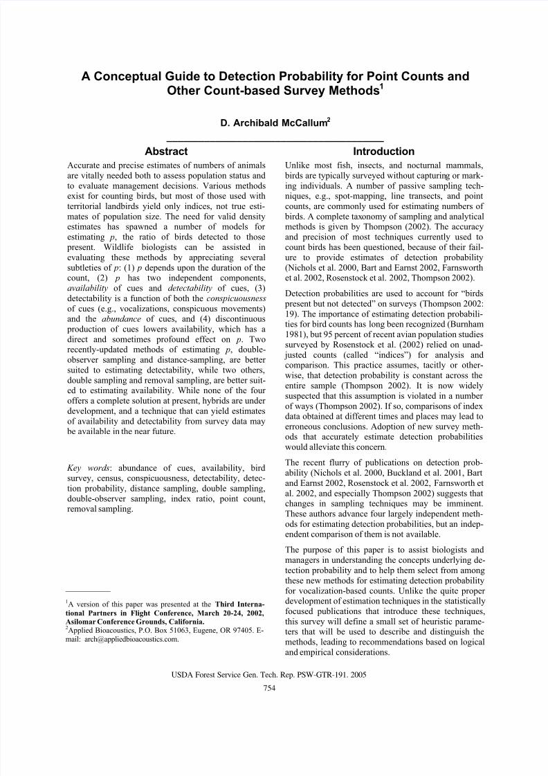
Figure 1 is a standard accumulation curve that shows

the cumulative number of individuals, C , detected for

any amount of effort, e.g., minutes (m) spent counting.According to this uncontroversial relationship, C is ex-

pected to be slightly higher in a 5-min point count thanit is in a 3-min point count, and considerably higher in2 hr of observation. The practice of sampling until the

cumulative count of individuals in an area levels off is

merely an empirical way to maximize detection of all

birds present (but the longer the count period, the

greater the likelihood of over counting, see below).

The curve in Figure 1 has the general form pm = 1-(1- p1m)m, where m is the duration of the count, pm is es-

timated by C/N for counts of that duration, and p1m is

the detection probability for a 1-min count. For example, if C/N = 0.5 for 3-min counts, p1m is 0.207. Once

p1m has been found, pm for count periods of any dur-

ation, m, can be calculated, and applied as a correction

factor to counts of that duration. This approach requiresindependent knowledge of N in the count areas in

which pm is estimated, as obtained with double samp-

ling methods (Bart and Earnst 2002).

2. For aural surveys, p must estimate both

“availability” and “detectability”

Although detectability of birds is a potentially a

function of a number of factors, it is useful for auralsurveys to subdivide p into two main components

(Farnsworth et al. 2002):

p = p s pd|s (2)

where p s is the probability that an average bird sings

(or produces some other detectable cue) and pd|s is the

probability it is detected, given that it sings. Recogniz-

0

2

4

6

8

10

12

0 50 100 150

Minutes (m )

C u m u l a t i v e C o u n t ( C )

Figure 1—Hypothetical cumulative count (C) of individuals

as a function of effort, e.g., minutes (m), in any kind ofmonitoring program. Detection probability, p = C/N, inc-reases with effort (e.g., total person-minutes) until all ind-ividuals are counted.


755




ing the distinction between these two component probabilities, “availability” and “detectability,” plays a

central role in evaluating the four methods (see below).

The next two sections explain each of these probabil-

ities.

3. Detectability: Only one detection is required tocount an individual

Unlike intensive survey methods, (e.g., territory-mapping, nest-finding protocols), “rapid survey” methods

(e.g., point counts, line transects) define a single det-

ection of an individual as sufficient to count that indiv-idual. Further detections of that individual do not

change C . Indeed, count periods are intentionally made

brief to minimize the possibility of double-counting of

an individual (e.g., Buckland et al. 2001). So, detect-ability ( pd | s) is actually the probability that a bird will

be detected at least once during its active periods.

Therefore

pd|s = 1-(1- p1d ) s (3)

where p1d is the probability of detecting an average cue;

and s is the number of cues, i.e., songs or other detect-

able acts, it actually produces during the count period.

Conspicuousness. P 1d is a measure of conspicuous-

ness, i.e., it captures reductions in detectability due

to the following four factors:

Amplitude of the vocalizations of the average individ-ual. Amplitude diminishes as the square of the distance

between the source and the detector, so detectability is

strongly influenced by distance and correlated factors,

such as sound blocking structures.

Auditory acuity of the observer. Acuity is frequency-dependent in all humans, and is greatest at 1-2 kHz,

below the frequencies of most bird sounds. One reason

that p differs among species is the varying degree to

which the birds’ sounds fall outside this 1-2 kHz band.

Moreover, individual humans vary in both general ac-uity and frequency response (Emlen and DeJong 1981).

Obviously, p is observer-specific for these reasons,

even if not for others.

Attentiveness of the observer. Because point countsare typically conducted in real time, i.e., the observer

cannot rewind and hear or see any cues a second time,

it is standard practice for an observer to attempt to fo-

cus on a single singer, identify it, and then move on to

another. This means that the listening time of the ob-server is divided among all the singers, some of which

will be missed if they cease vocalizing before the ob-

server has a chance to attend to them.

Masking of focal sounds by other sounds, includingambient noise, speech of the observer and any assist-

ants present, vocalizations of other species, and vocal-izations of non-focal individuals of the focal species.

High amplitude mitigates the other three causes. If a

sound is loud, it is more likely to be noticed and more

likely to mask other sounds then to be masked. Ampli-

tude is directly related to distance, while the other threefactors come into play because of the low amplitude of

sounds from distant sources.

Abundance of Cues. Parameter s is the number of

cues produced during a count period, independent

of their intensity. High singing rates ( s/m) mitigate

all four causes of non-detection, by giving the obser-

ver multiple opportunities to make the single detec-

tion that is needed to count an individual.

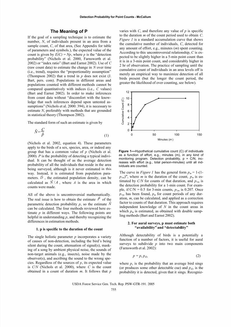
Equation (3) quantifies the intuitive relationship bet-

ween singing rate and the likelihood of detecting anindividual. The good news from this equation is that

even inconspicuous cues (low p1d ) can result in detect-ion when they are numerous (high s). For example, p1d

= 0.2, as one might find during an intense dawn chorus,

translates to pd | s = 0.996, with a realistic s of 25, or five

songs per min in a 5-min count period. Equation 3 also

shows why the dawn chorus may not be the optimal

time to conduct a survey. Singing rates ( s/m) tend to behighest at this time, and owing to correlation of s

among individuals, masking by other individuals may

reduce p1d , offsetting the advantage of high s. Figure 2

shows these trade-offs graphically.

0

0.2

0.4

0.6

0.8

1

1.2

0 5 10 15 20 25

Cumulative Songs (s ) in Count Period

D e t e c t a b i l i t y ( p d | s

)

Figure 2—Probability of detecting an individual at least

once during a count period as a function of the abundanceof cues (e.g., the cumulative number of songs it sings, s),and the conspicuousness of a cue (i.e., the probability ofdetecting it once, p1d ). Each curve represents a differentlevel of conspicuousness. A horizontal line anywhere onthis graph crosses combinations of conspicuousness andcue abundance (i.e., p1d and s) that yield identical detect-ability (pd|s).


756




0

0.2

0.4

0.6

0.8

1

1.2

0 5 10 15 20 25 30

Songs (s )

p = p s

p d | s

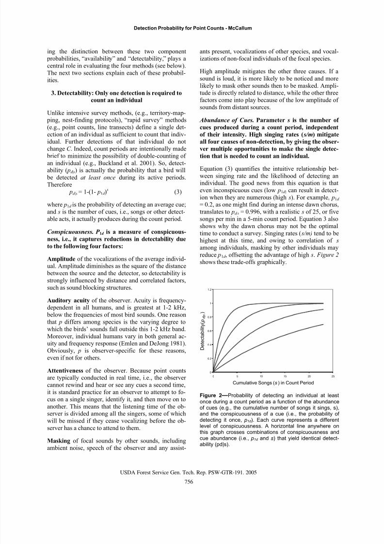
Figure 3—The joint effects of availability and detectabilityon detection probability ( p). Conspicuousness ( p1d ) is 0.40in all cases. The top curve is identical to the top curve inFigure 2. The other curves show the effects of lower avail-ability on overall detection, as singing males acquire matesand sing less often.

4. Availability: The overlooked componentof detection probability .

Availability, the probability that a bird produces any

cue at all during a count period, is often <1, and low

availability may be the most serious cause of non-detection. Surveyors use scheduling to mitigate the low

incidence of singing in the middle of the day, or late inthe breeding season, but optimal timing is not possible

for every sample. A correction for low availability due

to time of day, season, or pairing status would greatly

improve the accuracy of count data. Nonetheless, p has

been estimated as though it were a single parameter

until recently. Buckland et al. (2001) briefly referred toavailability, but did not include it as an independent

parameter in their model. Farnsworth et al. (2002) werethe first to do this.

Equation 3 and Figure 2 show that the probability ofdetecting an individual bird increases as its song pro-

duction, s, increases. This is, however, not the whole

story. If songs are evenly distributed across the time

period in which a survey may be taken, s should be agood predictor of detection. But, if songs are clumped

in time, i.e., delivered in bouts, silent intervals between

bouts may be long enough to completely overlap astandard count period. The resulting reduction in p s has

a serious impact on overall detection, p ( fig. 3).

Substituting equation 3 in equation 2, we have

p = p s (1-(1- p1d ) s) (4)

Because p s is independent of pd|s (Farnsworth et al.2002) and is free to vary from 0 to 1, there is no nec-essary correlation between singing rate s/m and the

overall value of p. There may, however, be an empir-

ical correlation between singing rate and p s, (e.g., Scott

et al., in prep.), and this deserves further study.

Comparison and Evaluation of Models

The double-observer (Nichols et al. 2000), double-

sampling (Bart and Earnst 2002), distance sampling

(Buckland et al. 2001), and removal (Farnsworth et al.

2002) models have been proposed as methods forestimating p. Consumers (e.g., wildlife biologists) need

criteria for choosing among these methods. The heur-

istic decomposition of detection probability, p, into

several independent components makes it easier tocompare and evaluate these methods. To be sufficient

for estimating p, a method must explicitly or implicitly

estimate the parameters of equations 2-4.

Double-Observer Method

The double-observer method obtains an estimate of p

by comparing the numbers of birds detected by two

observers, who count the birds in the same area at the

same time. The second observer records the data forthe primary observer, and at the same time is expected

to detect additional birds that are missed by the primary

observer. The method proposed for point counts is an

adaptation of a technique originally designed for visual

surveys from an aerial platform (Cook and Jacobson1979). It is a member of a family of “multiple-plat-

form” techniques (Buckland et al. 2001).

In actuality, the double-observer method (Nichols et

al. 2000) produces an estimate of pd|s that incorporatesthe effects of observer skill, inattention, and noise of all

kinds. The method offers no means of estimating p s,

and so tacitly assumes that p s = 1. The authors who applied it to point count data have subsequently endorsed

this interpretation (Farnsworth et al. 2002). It thereforeshould be used only in situations in which this as-

sumption can be met.

Distance Sampling

Distance sampling uses the fall-off in detections with

distance to model a distance-detection function for

plots with preset dimensions. The plot may be sampledfrom fixed points or a transect line. This function is es-

timated from the estimated distances to the first de-

tection of each individual per species. The distance-detection function is used to estimate a detection prob-

ability, which is construed (Buckland et al. 2001:37,

equation 2.2) to be p, as defined here. Density, D, is

estimated directly from p and A. N ˆ is calculated as

D̂ * A.

Distance sampling was developed to deal with the

effect of distance on visibility during ship-borne andairborne line-transect surveys of cetaceans. The line-

transect theory has been extended, with appropriate


757




modification for differences in geometry, to “pointtransects,” which are sets of variable circular plot sur-

veys (Ramsey and Scott 1979, Reynolds et al. 1980),

with updated estimation methods (Buckland et al.

2001).

Although distance sampling has been proposed forsurveying territorial songbird populations (Buckland et

al. 2001, Rosenstock et al. 2002), this recommendation

comes with a number of caveats and disclaimers. A

very clear assumption of the method is that all animals

present at distance = 0 are detected. Leaving aside thevery real possibility that the observer’s presence may

bias detection or even the presence of animals at closedistances, this assumption tacitly requires that p s = 1,

i.e., that all animals present perform detectable acts

during the survey period. The detection probability es-

timated by the distance method is therefore pd|s, not p.

When cues are discrete, e.g., bird song, the assumption

of perfect detectability at distance = 0 may be difficultto meet. This can be mitigated by increasing the time at

the point. But, “the objects around a point should be

located at an instant in time” (Buckland et al.2001:147). These authors recommend a “snapshot”

preceded by a few minutes of locating individuals and

followed by a few minutes to confirm their presence at

the time of the snapshot. If birds are counted through-out the period, as is typical in point counts, an upward

bias in the estimate of numbers results.

Incidentally, if the recommended snapshot is essen-

tially instantaneous, does it estimate pd|s or p1d , in the

terminology of this paper (see equation 3)? Actually,the two are equal when s = 1, as is the case in an

instantaneous sample. Moreover, because the estimate

of C is also instantaneous, the constant ratio of C and p

discussed above is not violated.

Bout structure also poses problems. When “periods ofdetectability [are] interspersed with periods of unavail-

ability” the distance method produces an estimate that

is the product of density and the proportion of birds

available for detection [i.e., p s] at any given time(Buckland et al. 2001:189). This is a second way of

saying that the distance method estimates pd|s, not p. In

such circumstances, e.g., whales that dive for long

periods or songbirds that are silent for periods longerthan the standard counting period, an independentestimate of p s is required.

An alternative to conventional distance sampling is

“cue counting,” in which distance is estimated to every

cue (song or other detectable event) rather than everyanimal. In this case, movement of the bird is not a

problem, as long as all cues are counted. The detection

function is estimated as with distance sampling, and the

estimate of D requires an independent estimate of cue

rate, which is s/m in the terminology of this paper. Thisis a possible area of research (Buckland et al. 2001).

Potential difficulties are detecting and measuring dis-

tances to all the cues in a chorus of songbirds, and high

variance in the cue rate owing to bout structure (seeabove).

Despite these difficulties, distance sampling does offer

a potential solution to a major problem of point counts.

The probability of detecting a single song, p1d , is a

function of the amplitude of the song and related

factors (see above). Because amplitude decreases as thesquare of distance increases, each bird would have a

different p1d . A method is needed to account for p1d forthe entire population, and the distance method would

appear to meet this need.

Double Sampling

The double-sampling model was developed for water-

fowl monitoring and has been adapted to the moni-

toring of breeding populations of upland birds (Bartand Earnst 2002). Unlike the other three models,

double-sampling does not attempt to estimate p from

the data to which it will be applied as a correctionfactor. A set of “rapid surveys,” such as line-transects

or variable circular plot counts, is taken as usual. In a

random subset of the rapid survey plots, other workers

conduct “intensive surveys,” i.e., true censuses of all N

individuals present. The estimate of p obtained from

the ratio C/N in the intensive plots may then be used asthe estimate of p for the rapid surveys.

To date, the main empirical shortcoming of this method

is that it has not yet been applied to point-centered

rapid surveys. The rapid surveys performed by Bartand Earnst (2002) involved area search, rather than

aural sampling, in tundra (i.e., treeless) study plots,

where the attenuation of a bird’s signal with distance

was a negligible problem. These relatively long “rapid”surveys in areas with relatively low bird density and

high visibility made masking and inattention insignif-

icant issues. But, application of double-sampling toaurally based point counts in areas with more complex

vegetation will require an estimate of pd|s. It may be

that an adequate estimate of pd|s can be obtained withthe distance method.

Intensive surveys of birds typically include nest

searches and territory mapping. Territory mapping isessential to determine whether the territory centroid is

on or off the measured intensive plot, and must be done

just outside as well as inside the plot for this reason(Bart and Earnst 2002). Although highly desirable, in-

tensive study plots can be expensive to census. Bart

and Earnst (2002) provided estimators of cost, and a


758




routine for optimizing allocation of effort to intensiveand rapid plots.

Removal Sampling

In developing their removal model, Farnsworth et al.(2002) explicitly set out to overcome the shortcomings

of the double-observer and distance methods by ac-counting for p s as well as pd|s. This is a large step in the

right direction. Their approach relies on the logic of

removal sampling, in which the probability of trappinganother individual declines as individuals are removed

from a closed, finite population. The method of

Farnsworth et al. (2002) relies on “virtual” removal.

They divide a point count period into sequential seg-ments, and record the number of birds first detected in

each segment. The decline in new detections over the

duration of the count is used to estimate p s. The com-

putational gambit that permits an estimate of p s without

knowing N is division of the N birds into one ad hocsubgroup in which all birds are detected and another in

which some are detected. This assumption is relaxed insome reduced models.

Despite providing the first explicit decomposition of

detection probability into availability and detectability,the model of Farnsworth et al. (2002) estimates only

availability. Nevertheless, this model makes it possible

to reanalyze old data sets that are subdivided tem- porally and produce an estimate of detection prob-

ability.

More recently, Farnsworth et al. (this volume) haveadded a distance component to their removal model, as

suggested by Farnsworth et al. (2002). They estimatedetectability ( pd|s) by dividing the count circle into two

or more concentric rings, and assigning the first de-

tection of each individual that is counted to one ofthese rings. This practice yields an estimate of detect-

ability for the entire circle that is corrected for the fall-

off in detectability with distance. This “binning” of the

data into concentric rings is an acceptable alternative toestimating the distance to each bird as long as birds are

accurately assigned to rings (Buckland et al. 2002,

Farnsworth et al. 2002).

Farnsworth and colleagues are seeking a method thatcan be applied retrospectively to point count data thatwere binned into time intervals and distance rings. For

example, Ralph et al. (1995) recommended recording

data separately for sequential 3-, 2-, and 5-min seg-

ments of a 10-min point count, so the results can be

compared to BBS results, which are based on 3-min point counts, and other data sets. Similarly, the recently

adopted protocol in the U. S. Pacific Northwest (Huff

et al. 2000) recommends subdividing detections into atleast two distance rings. Many data sets may therefore

yield estimates of availability and detectability if thisremoval-distance method proves reliable.

Because this method is intended to estimate both avail-

ability and detectability from actual count data, without

the expense of double-sampling, managers will follow

its development with great interest. A few cautions aretherefore in order.

The cues produced by territorial birds are often deli-vered in bouts of intense singing separated by intervals

of total silence. This bout structure is a challenge for

the removal method. Availability is estimated fromchanges in activity during count periods. In the most

likely case, a 5-min count divided into 3-min and 2-

min segments, some segment of the population must

stop or start producing cues during that short interval.Availability will be overestimated as 1.0 if all indi-

viduals present are either silent or active throughout the

5-min count period. The longer are the bouts and inter-

bout intervals, the greater this problem becomes. The proportion of the N individuals that must start or stop

producing cues in order to yield an accurate estimate of

availability is therefore a question that must be ad-dressed.

Adding the distance method to the removal method isexactly what is needed to estimate detectability. But the

requirement that the count be taken at an instant in time

(see above) poses a problem for the method of Farns-

worth et al. (this volume), which relies on changes inactivity during a count period to estimate availability.

Buckland et al. (2001, see discussion above) recom-

mend sandwiching a “snapshot” between brief periods,in which active birds are accounted for, to obtain the

instantaneous count. Perhaps such a “snapshot” can be

taken during each of the time segments, thereby

yielding the estimate of availability without compro-

mising the estimate of detectability. This issue illus-trates well the heuristic value of distinguishing between

availability and detectability.

In summary, concern about this method does not center

on the use of concentric distance rings, which is a well-understood alternative to estimating distance to each

bird, but instead on the applicability of the distance

method, in any form, to point counts that rely on aural

cues. Nevertheless, because the removal-distancemethod is conceptually adequate (i.e., it recognizes theindependence of availability and detectability) and

mathematically rigorous, it deserves thorough study,

with the hope that it proves robust to the caveatsexpressed above.


759




Conclusions

In conclusion, all four methods reviewed appear logic-

ally valid, when their stated and unstated assumptions

are met. The currently predominant method for survey-

ing songbirds, rapid aural point counts, will seldom

meet all the assumptions or requirements of any ofthese methods. In their current forms, the double-obser-

ver and distance-sampling methods are better suited to

estimating detectability, while the double-sampling andremoval methods are better suited to estimating avail-

ability. Although incomplete at the time of this writing,

all four of the new methods probably yield less-biasedindices than raw point counts (Bart and Earnst 2002).

A hybrid of two, three, or all four of these methods is

the likely outcome of further development in this fast-

moving field.

AcknowledgmentsDiscussions with B. Peterjohn and K. Pardieck about

estimating detection probabilities from tape recordings

inspired this paper. I thank the authors listed below for

advancing the field with their penetrating insights. G.

Johnson, J. Bart, B. Walker, and C. J. Ralph kindly

reviewed the manuscript and provided much neededfeedback

Literature CitedBart, J. and S. Earnst. 2002. Double sampling to estimate

density and population trends in birds. Auk 119: 36-45.

Buckland, S. T., D. R. Anderson, K. P. Burnham, J. L. Laake, D.L. Borchers, and L. Thomas. 2001. Introduction to dis-

tance sampling: Estimating abundance of biologicalpopulations. Oxford, UK: Oxford University Press.

Burnham, K. P. 1981. Summarizing remarks: Environmental

influences. Studies in Avian Biology 6: 324-325.

Cook, R. D. and J. O. Jacobosen. 1979. A method for estim-

ating visibility bias in aerial surveys. Biometrics 35: 735-742.

Emlen, J. T. and M. J. DeJong. 1981. The application of song

detection threshold distance to census operations.Studies in Avian Biology No. 6: 346-352

Farnsworth, G. L., K. H. Pollock, J. D. Nichols, T. R. Simons, J.E. Hines, and J. R. Sauer. 2002. A removal model for

estimating detection probabilities from point-countsurveys. Auk 119: 414-425. Estimating density from

point-count surveys: theory with applications.

Farnsworth, G. L., J. D. Nichols, J. R. Sauer, S. G. Fancy, K. H.Pollock, S. A. Shriner, and T. R. Simons. This volume.

Statistical approaches to the analysis of point-countdata: a little extra information can go a long way.

Huff, M. H., K. A. Bettinger, H. L. Ferguson, M. J. Brown, andB. Altman. 2000. A habitat-based point-count protocol

for terrestrial birds, emphasizing Washington andOregon. Gen. Tech. Rep. PNW-GTR-501. Portland, OR;Pacific Northwest Research Station, Forest Service, U.S.Department of Agriculture; 39 p.

Nichols, J. T., J. E. Hines, J. R. Sauer, F. W. Fallon, J. E. Fallon,and P. J. Heglund. 2000. A double-observer approach for

estimating detection probability and abundance frompoint counts. Auk 117: 393-408.

Ralph, C. J., J. R. Sauer, and S. Droege. 1995. Monitoring bird

populations by point counts. Gen. Tech. Rep. PSW-GTR-129. Albany, CA: Pacific Southwest Research Station,Forest Service, U.S. Department of Agriculture.

Ramsey, F. L. and J. M. Scott. 1979. Estimating population

densities from variable circular plot surveys., In: R. M.Cormack, J. P. Patil, and D. S. Robson, editors. Sampling

biological populations. Fairland, MD: International Coop-erative Publishing House; 155-181.

Reynolds, R. T., J. M. Scott, and R. M. Nussbaum. 1980. A

variable circular-plot method for estimating bird

numbers. Condor 82: 309-313.

Rosenstock, S. S., D. R. Anderson, K. M. Giesen, T. Leukering,and M. F. Carter. 2002. Landbird counting techniques:

Current practices and an alternative. Auk 119: 46-53.

Scott, T. A., P.-Y. Lee, G. Greene, and D. A. Mccallum. Thisvolume. Singing rate and detection probability: an

example from the Least Bell’s Vireo (Vireo belli

pusillus).

Thompson, W. T. 2002. Toward reliable bird surveys:

accounting for individuals present but not detected. Auk119: 18-25.


760




Appendix 1. Detection Probability Cheat Sheet

Parameters discussed in this paper, and their algebraic symbols, if used.

Symbol Parameter

A Area. The measured area of a survey area.

C Count. The number of individuals detected by some survey method in a single count area, or group ofsuch areas.

D Density. The number of resident individuals per unit area. D̂ is often estimated as N ˆ / A, but it is the primary output of the distance method.

M Time. As used here, the number of minutes in a single point count or other sample.

N Population size. The number of individuals, or males, or other category of interest, that reside in a

survey area. If the area is small, e.g., a point count circle, care must be taken to account for home

ranges that are not wholly included in the area. One approach to this problem is to consider anindividual a resident of a survey area if the centroid of its territory or home range lies inside the

boundaries of the area (Bart and Earnst 2002). ˆ is an estimate of N that is calculated from estimatesof other parameters. It is the primary output of the double observer and double sample methods.

p Detection Probability. The likelihood that a typical (average) individual residing in a survey area will

be detected at least once during a survey period. Synonym of Index Ratio. P ˆ

is an estimate of p that is produced by all four methods described in this paper.

pd|s Detectability. The likelihood that at least one cue (a behavior that is physically detectable by the

means employed in the survey) is detected during the count period of m minutes. ps Availability. The likelihood that an individual residing in a survey area produces a cue during the

survey period.

p1d Conspicuousness. The absolute energy content of a cue, at the survey point, discounted by the

conspicuousness of competing cues. The probability that an average cue is detected.S Cue Abundance. The number of cues available for detection during a survey period. High cue

abundance mitigates the effect of low conspicuousness.

s/m Cue Rate. The number of cues occurring per unit time.s/m Song Rate. The number of songs occurring per unit time. A special case of Cue Rate.

Cue. Any discrete behavior (e.g., a song, a display flight) that can be used, with appropriate

equipment, to detect a bird. When evidence of the presence of a bird comes in packets, rather than

continuously, each packet is a Cue.


761

Documents

Guide to Detection Probability for Point Counts