Embed Size (px)
Citation preview

1
Small or medium-scale focused research project (STREP)
ICT Call 8 FP7-ICT-2011-8
Cooperative Self-Organizing System for low Carbon Mobility at low Penetration Rates
Guideline for emission optimised
traffic light control

2
Document Information
Title Guideline for emission optimised traffic light control
Dissemination Level PU (Public)
Version 1.0
Date 03.11.2015
Status Draft / Approved by Coordinator
Authors Martin Dippold (TUG), Stefan Hausberger (TUG), Nikolaus Furian
(TUG), Michael Haberl (TUG), Jakob Hauser (TUG), Thomas Stützle
(ULB), Wolfgang Niebel (DLR)
3
Abbreviations and symbols
Name Unit Description
BEV Battery Electric Vehicle
CO g Carbon monoxide
CO2 g Carbon dioxide
FC g Fuel consumption
HBEFA Handbook Emission Factors for Road Transport
HBS Handbuch für die Bemessung von Straßenverkehrsanlagen
HC g Carbon hydride
HCM Highway Capacity Manual
HEV Hybrid Electric Vehicle
I2V Infrastructure to vehicle communication
ISV Institute for Highway Engineering and Transport Planning
IVT Institute for Internal Combustion Engines and Thermodynamics
LoS Level of Service
MONITRA Monitoring and optimizing Traffic signalization
NOx g Nitrogen oxide
NS # Number of stops
PHEM Passenger Car and Heavy duty Emission Model
PHEV Plug-in Hybrid Electric Vehicle
PI Performance Indicator
PM g Particle mass
QSV Qualitätsstufen des Verkehrsablaufs (quality level of traffic flow)
SUMO Simulation of Urban Mobility
TLC Traffic Light Control
TT s Travel time
UTC Urban Traffic Control
v m/s velocity
v_avg m/s Average velocity over a trip or on a road section
V2X Vehicle to vehicle and vehicle to infrastructure communication
WT s Waiting time
Definitions
Name Description
Cycle time/ length See chapter 2
Green split See chapter 2
Intergreen matrix Collects intergreen times which are the intervals between the end of one
green time of a signal group and the start of the green time of the next signal
group
Offset See chapter 2
Phase (AE) = Stage
(BE)
For traffic lights the term phase/ stage means a set of compatible signal
groups which may have green at the same periods but the timings of green
begin and green end may not be identical
Traffic stream or
approach (access) All lanes of traffic that enter the intersection from the same direction

4
CONTENT
Inhalt
1 Introduction ......................................................................................................................... 5
2 TLC parameters and their optimisation potential ............................................................... 6
3 Optimisation of TLC for low emissions ............................................................................. 6
3.1 Coordination of traffic lights on arterial roads for low emission levels ...................... 9
4 Existing Traffic Engineering Planning Software .............................................................. 10
4.1 Tools for TLC design and microscopic traffic simulation ........................................ 10
4.2 Tools for Emission Simulation .................................................................................. 11
4.2.1 PHEM ................................................................................................................. 11
4.2.2 PHEMlight ......................................................................................................... 11
4.2.3 VERSIT+ ............................................................................................................ 11
4.2.4 HBEFA ............................................................................................................... 12
4.2.5 COPERT ............................................................................................................. 12
4.3 Optimisation Tools .................................................................................................... 12
4.3.1 Traffic and emission simulation Tool MONITRA ............................................. 12
4.3.2 Others ................................................................................................................. 13
5 Summary ........................................................................................................................... 14
6 References ......................................................................................................................... 16
7 ANNEX ............................................................................................................................. 17
7.1 Application of MONITRA ........................................................................................ 17
7.1.1 Calibration .......................................................................................................... 19
7.1.2 Optimising routine in MONITRA ...................................................................... 20
7.1.3 Results from MONITRA .................................................................................... 22

5
1 Introduction
Traffic signal control has become an important operational measure of road traffic
management, in particular as it has become more and more difficult to provide sufficient road
space despite growing traffic demand. Since traffic signal systems directly intervene in traffic
by alternatively stopping or releasing traffic flows which share conflict zones, they have to be
designed, implemented and operated very carefully.
The design of a traffic signal system covers the selection of the control strategy, the traffic
engineering description of control, the ca1culation of the signal program elements as well as
the road traffic engineering design of the intersection, road section or part of a network
inc1uding the corresponding traffic control measures.
Optimization of intersection signal timing theory was initiated in the 1950s. Webster was the
first to introduce a method to optimise intersection signal timing targeting at minimizing
delay. Besides delay also stops and capacity were added into objective functions as
performance indicators. The traffic signal control researches are mostly based on average
delay, number of queuing vehicles, stops, intersection saturation degree and capacity, etc.
Emissions usually are not included in the traffic signal control metrics.
The general steps of traffic light planning for fixed time control are the following:
1. Determination of the traffic volumes: Analysis and forecast of the expected traffic
volumes.
2. Definition of geometrical parameters: Number of lanes, geometry of intersections.
3. Determination of the intergreen matrix as function of geometry.
4. Determination of phases: Number of phases, possible phase sequences.
5. Creation of the signal program: traffic volumes of streams per lane, saturation of
streams, cycle length, green time for each phase (green split), offset in coordination.
6. Proof of the capacity and quality of traffic flow using parameters such as QSV or LoS.
The result of these planning steps is a traffic light control algorithm that generates a specific
traffic flow. Main parameters for the optimisation are the green split and the offset in step 5.
The resulting traffic flow can be distinguished at least into acceleration, cruising, deceleration,
and stop time which leads to specific emission effects. Each deceleration by using the
mechanical brakes annihilates energy which afterwards has to be delivered by the engine to
accelerate again. Stop times add emissions without covering a distance and different speed
levels result in different driving resistance losses. Also the acceleration levels are relevant for
the actual engine power demand and thus for the engine efficiency and for the emission
levels. By the development of the traffic control algorithms all of these effects should be
considered by the traffic engineer to achieve low emissions and minimum fuel consumption.
Consequently this guideline was produced to give the traffic engineer an overview on rules to
be followed and on supporting tools available to consider emission effects.

6
2 TLC parameters and their optimisation potential
The main parameters controlling the operation of a signalized intersection are the cycle time,
the green split for the different approaches of the intersection and the offset.
Cycle Time (Cycle Length): The cycle time is defined as the sum of the durations of
all distinct phases of the signalized intersection. Cycle lengths must be the same for all
junctions in the coordination plan to maintain a consistent time based relationship. To
find the optimum cycle time, the goal is to minimize the average vehicle delay.
Efficiency dictates that the cycle length should be long enough to serve all of the
critical movements, but no longer.
Figure 1: Schematic interaction of Cycle Time and Delay Time
Most existing intersection signals are based on delay minimization. However,
minimizing delay does not necessarily lead to the minimization of emissions at an
intersection.
Green split/ Green time (Green period): The green split for a given approach is
defined as the ratio between the amount of green time and the cycle time. The green
time is the duration of the green display for a stage or a movement. The green time is
usually divided among the different traffic streams according to traffic intensity for
each stream. Minimum green defines the shortest allowable duration of the green
interval due to safety reasons.
Offset: The offset of a signalized intersection is defined as the difference in time
between the start of a cycle of this intersection and the start of a cycle of some
reference intersection. It is used to provide signal coordination between consecutive
intersections; the latter is usually accomplished through the use of a common cycle
time (which may change over time). The offset depends on the distance between
signals, the progression speed along the road between the signals and the queues of
vehicles waiting at the red signal.
3 Optimisation of TLC for low emissions
Typically control algorithms are optimised for kinematic parameters, such as number of
vehicle stops and travel times. With the availability of robust microscopic emission models
(chapter 4.2) optimisation for low environmental impacts is an emerging issue. Since optima
for kinematic parameters are not necessarily leading to low emission levels (chapter 7.1.3) it
is worth to test or to optimise effects on CO2 and on the most relevant pollutant emissions
(usually NOx and PM due to the exceeding of corresponding air quality limits).

7
Beside the application of comprehensive modelling already the consideration of basic rules
for emission impacts can help to avoid worse emission effects.
In the basic consideration driving can be distinguished into following phases:
Acceleration
Cruising (approx. constant speed)
Deceleration
Stop time.
Ideal emission case is “cruising” at velocities between 40 and 80 km/h. Emissions per km are
typically more than twice as high for a stop and acceleration events. In road networks
however, it is usually not possible to maintain constant speed for all vehicles. Emissions can
be reduced by the driver and by traffic light control systems.
The design of the control system should mainly aim at minimizing the demand for mechanical
braking and for harsh acceleration. The effects are summarized in Table 1. A more detailed
analysis can be found in [COLOMBO D4.3, 2014].
Table 1: Overall rules for traffic flow strategies for optimal driving behaviour for low emissions
Driving event Emission influence Emission optimal
Cruising Different speed levels result
in different driving resistance
losses and different engine
efficiencies.
Best fleet emissions in the velocity range of
about 40 km/h to 80 km/h.
Acceleration Acceleration always needs
more energy than cruising.
Consequently also most
exhaust gas components are
much higher per km.
Rather slow or moderate acceleration
behavior is favorable in terms of emission
optimization (30% till 50% of the engine
load).
Deceleration Mechanical braking converts
useful kinetic energy into
useless heat. Thus any
mechanical braking shall be
avoided whenever possible.
Optimal deceleration uses the air and
rolling resistance to reduce kinetic energy
of the vehicle without any mechanical
braking (i.e. coasting). Typical values (1)
are:
Passenger cars -0.3 m/s² to -0.6 m/s²
Heavy duty vehicles -0.5 to -1.4 m/s²
In practical use deceleration by just
coasting without brake pedal activation
leads to lowest emissions.
Stops Stop times add emissions
without covering a distance.
Should always be avoided but less
pronounced impact with increasing share of
vehicles with start/stop systems (2)
.
Typically longer idling times lead to less
overall emissions than more braking
events.
(1) Deceleration for coasting conditions depends mainly on actual velocity (higher air resistance at higher
speeds), vehicle aerodynamic design and mass and road gradients.

8
(2) Auxiliaries are fed by the battery during engine stop. This energy has to be produced by the alternator
later under engine operation and increases emissions to some extent there.
The optimum driver behavior is:
1. Drive as steady as possible (“cruising”) in a velocity range of 40 km/h to 80 km/h.
2. Choose the highest possible gear in order to keep the engine speed low (but above about
1.5 times the engine idling speed).
3. Drive as “anticipating” as possible in order to avoid the use of mechanical brakes as
much as possible.
4. Perform decelerations in engine motoring mode (i.e. without additional mechanical
braking) and using a high gear. Shift back when engine speed comes close to engine
idling speed.
5. Accelerate in a moderate way using high gears.
6. Avoid stop times with running engine.
For the hybrid vehicles all above made statements are also found to be correct. Since the
hybrids recuperate parts of the brake energy, mechanical braking means lower losses of
energy than for conventional vehicles.
Approaches for optimising traffic light control systems exist for different levels:
Single traffic light
Interaction between traffic lights (e.g. “green wave”)
Overall road network influenced by traffic lights.
Suitable models have to provide a combination of traffic simulation and emission simulation.
Since the emissions depend very much on microscopic events such as accelerations and
decelerations, average speed based approaches usually cannot provide a sufficient resolution
to find optima. Thus the simulation has to consider vehicle movements at least with resolution
to acceleration, deceleration, cruise and stop. Consequently a combination of microscopic
traffic models (e.g. SUMO, VISSIM, AIMSUN, etc.) with microscopic emission models
(PHEM, PHEMlight, VERSIT+, see chapter 4.2) is an attractive approach.
Implementing the emission model directly into the traffic model allows straight forward
optimization loops for variations of traffic light control parameters. A corresponding model
with PHEMlight integrated into SUMO is shown in [COLOMBO D5.3, 2014].
Such tools can be used by traffic engineers to simulate the road network with different
settings of the traffic light control and analyze effects on average travel time, stops, fuel
consumption and emissions.
Within the COLOMBO project, we have developed a traffic light control algorithm based on
swarm intelligence principles. The behaviour of this algorithm can be optimized for a single
intersection or for a road network when used within a simulation-based optimization
framework. As optimization goals can be set arbitrary objectives such as waiting time, the
number of stops, or the amount of emissions or weighted combinations of these. Hence, also
emission minimization can be achieved, which was done within the COLOMBO project using
the integration of PHEMlight into SUMO. More details on the simulation-based optimization
framework that we have created are given in Section 4.4 of these guidelines.

9
In the following, we give an overview on the coordination of traffic lights on arterial roads.
3.1 Coordination of traffic lights on arterial roads for low emission levels
If traffic flow does exist just in one direction, the offsets of green light phases between the
single traffic lights can be calculated by using simple software or even by using a set of basic
equations as shown in [COLOMBO D4.3, 2014]. The correct consideration of vehicles
entering from side roads can be important in such cases to avoid unnecessary braking
demands for vehicles on the main road.
As soon as several traffic lights are coordinated along a road and traffic is running in both
directions the optimisation of traffic light control algorithms for low emission levels is
becoming a very complex task. Achieving green waves without interruption for both
directions is typically even in theory impossible due to different vehicle speeds, inconstant
distances between traffic lights and necessary green phases for intersecting vehicles.
Additionally vehicles turning left or right from the main road can disturb the traffic flow as
well as pedestrians etc.
Parameters to be adjusted in principle for each single traffic light are
(a) Duration for green and red light per direction for cars and pedestrians (with boundary
conditions to be met for safety reasons)
Parameters to be optimised for all traffic lights are
(b) Offset between consecutive traffic lights
Since the optimum for (b) depends on the settings in (a), the best solution most likely can be
achieved by iterative variations of (a) and (b) parameters considering some basic boundary
conditions, e.g. equal cycle times for each traffic light [RiLSA, 2010].
To optimise the remaining parameters for emissions and/or for kinematic parameters the
support by suitable simulation tools is highly recommended. Such tools cannot replace
experience and brainpower of the engineers but can help a lot to further improve the
understanding of emission related effects.
A simplified tool was elaborated within the COLOMBO project which has lower demands to
set up the model than microscopic traffic models and which includes PHEMlight for emission
simulation and an optimization routine (MONITRA, chapter 4.3).
An example from an application of the tool MONITRA with optimization for different targets
is provided in the Annex (7.1.3). The optimization runs used three different parameter
settings:
(a) Equal weighting of “waiting time” and “number of stops” in the target function,
(b) Equal weighting of “CO2”, “waiting time” and “number of stops” in the target
function,
(c) CO2 optimization (100% weighting of CO2 in the target function)
The optimization algorithm looks for each parameter on the reduction rate against the base
case and looks for an optimum of the weighted average improvement of the parameters
according to the user defined weightings.
The simulation shows that an optimization for “waiting time” and “number of stops” does not
result in the lowest emission levels while a target function combining “waiting time”,

10
“number of stops” and CO2 emissions gives low values for all relevant parameters in this
example. Optimization for CO2 only results in increased travel time and waiting time which
however are still below the base case. Depending on the base case considered the reduction
potential by optimization given by MONITRA for this example is in the range of 10% for
emissions (chapter 7.1.3).
Certainly the potential for improvements depends on the actual status of the control algorithm.
In any case an assessment of the potential by simulation is suggested if local air quality
problems or overall CO2 reductions are a development task. Achieving 10% emission
reduction on local level by other measures often is more challenging. As discussed above the
optimization of kinematic parameters does not guarantee low emissions. Thus emission
simulation is necessary if well-founded results are required.
4 Existing Traffic Engineering Planning Software1
4.1 Tools for TLC design and microscopic traffic simulation
TLC design tools shall help traffic engineers to execute all necessary steps from junction
geometry mapping to upload files into the actual controller. Automatic calculations, checks
for violations of threshold values, and suggestions for meaningful signal plans are featured.
Most of available software is suitable for fixed-time and actuated control, while some
products also comprise adaptive algorithms (cf. [COLOMBO D2.2, 2014]). Different traffic
scenarios can be tested, and formula based evaluation according to procedures like the
German manual HBS or the US-American HCM delivers benchmarking performance
indicators (PIs) like QSV or LoS, respectively. Generic design tools yield in results which can
be implemented into any controller, but controllers also come with their own customized
implementation software. As urban corridor and network control (UTC) demands orchestrated
phase switches at multiple junctions, remote control from a central software will do the job.
Commercially available examples of such software packages are Ampel (BPS GmbH),
LISA+/INES+ (Schlothauer & Wauer), Sitraffic Office (Siemens), VS-Plus (Verkehrs-
Systeme AG), ImFlow (PEEK), and TRANSYT (TRL).
For sophisticated evaluation microscopic traffic simulation software can be applied. Most of
the times these products come with interfaces to at least one of the above mentioned planning
packages for the ease of data transfer and real-time interaction “in the loop”.
Common products are VISSIM (PTV), AIMSUN (TSS), Paramics (Quadstone), MATSim
(TU Berlin), and SUMO (DLR)2. The last two are available as open source. The evaluation
suite MAT.CrossCheck (MAT.Traffic) is designed to interact with VISSIM and comprises the
procedures of the HBS.
Since the shares in acceleration, deceleration, cruise and stop time over the trip are main
parameters defining the resulting emissions, the user of traffic simulation consequently has to
ensure that the driver behavior in these traffic situations is modelled in a representative way.
Thus a check of the acceleration and deceleration values simulated by comparison with real
world data is necessary.
COLOMBO made use of the SUMO simulation software to evaluate the directly implemented
TLC algorithm “SWARM” and the ImFlow algorithm.
1 An overview on existing traffic engineering software is also given in Deliverable5.3 of the COLOMBO project.
2 A non-exhaustive overview can be found on https://en.wikipedia.org/wiki/Traffic_simulation#Microscopic

11
4.2 Tools for Emission Simulation
As discussed before models used for emission simulation shall be instantaneous models if
effects from changes in traffic flow shall be assessed. Instantaneous models are defined by
considering changes in vehicle speed and acceleration over time or over distance with
approximately 1Hz resolution. Some instantaneous models exist, which allow calculating
representative vehicle fleet emissions. These models are shortly described below together
with other commonly used tools. Tools based on data from few vehicles only are not
recommended, since the emission behaviour between single vehicle makes and models differ
significantly (e.g. reports on www.hbefa.bet).
4.2.1 PHEM
PHEM (Passenger Car and Heavy duty Emission Model) is an emission map based
instantaneous emission model, which has been developed by TU Graz since the year 2000.
PHEM calculates the fuel consumption and emissions from road vehicles in 1Hz for any
driving cycles based on the vehicle longitudinal dynamics and emission maps. Road
gradients, different vehicle loading as well as e.g. warm up and cool down of exhaust gas
after-treatment systems are considered in the model. Data from more than 1000 measured
vehicles are compiled to provide average vehicle data sets. Based on this data PHEM includes
input data sets for all gasoline and diesel vehicles from EURO 0 to EURO 6 plus hybrid
electric vehicles (HEV), plug-in- hybrid electric vehicles (PHEV), battery electric vehicles
(BEV) for cars, LCV and HDV for different size classes. New technologies like start-stop
systems are also considered. The user can select the vehicle fleet composition and the driving
cycles to be calculated. Also amendments in the vehicle data can be done for special
applications. In the meantime PHEM is a standard tool for many countries and provides the
basic emission factors for the HBEFA and COPERT. A detailed description of PHEM can be
found e.g. in [Rexeis et al., 2013] and [COLOMBO D4.2, 2014].
4.2.2 PHEMlight
PHEMlight was developed in the COLOMBO project and was designed to be integrated into
SUMO. For the application within a micro-scale traffic model, several detailed simulations
from PHEM were replaced by generic functions using only information’s that are available
from traffic models for the second actually computed. The emissions are described in
PHEMlight as function of the wheel power only (no simulation of engine speeds). Also
exhaust gas after-treatment temperatures are not simulated. These detailed simulations were
replaced by average effects computed by PHEM for these parameters. The simplifications
lead to a fast, robust and low storage demand calculation with still good model accuracy.
Considering the uncertainties in vehicle speed simulation from the traffic models the
simplifications in PHEMlight do rather not have negative effects for the user. A detailed
description of PHEMlight can be found in [COLOMBO D4.2, 2014].
4.2.3 VERSIT+
For the simulation of hot running emissions, VERSIT+ LD uses a set of statistical models for
detailed vehicle categories that have been constructed using multiple linear regression
analysis based on a large number of vehicle emission tests. VERSIT+ has already been used
in different projects at different geographical levels. Compared to COPERT IV, the VERSIT+
average speed algorithms provide increased accuracy with respect to the prediction of
emissions in specific traffic situations [VERSIT, 2007]. Effects of road gradients and different
vehicle loading are not considered but instantaneous emission simulation is possible.

12
4.2.4 HBEFA
The Handbook of Emission Factors for Road Transport (HBEFA) was originally developed
on behalf of the Environmental Protection Agencies of Germany, Switzerland and Austria. In
the meantime, further countries (Sweden, Norway and France) as well as the JRC (European
Research Center of the European Commission) are supporting HBEFA. It provides emission
factors, i.e. the specific emission in g/km for all current vehicle categories (PC, LDV, HDV,
buses and motor cycles), each divided into different categories, for a wide variety of traffic
situations [www.hbefa.net]. An application of the HBEFA emission factors for the assessment
of emissions under different traffic light coordination systems is not recommended since
neither velocity nor acceleration values can be adjusted by the users. Since PHEM provides
the emission factors for HBEFA rather the use of PHEM or PHEMlight is recommended if
results shall be in line with the HBEFA emission values.
4.2.5 COPERT
COPERT 4 is a software tool used world-wide to calculate air pollutant and greenhouse gas
emission inventories from road transport. The development of COPERT is coordinated by the
European Environment Agency (EEA), in the framework of the activities of the European
Topic Centre for Air Pollution and Climate Change Mitigation. The European Commission's
Joint Research Centre manages the scientific development of the model. COPERT has been
developed for official road transport emission inventory preparation in EEA member
countries [COPERT, 2015]. Since COPERT simulates emissions as function of the average
speed of a cycle, the suitability for the assessment of emissions under different traffic light
coordination systems is limited. E.g. similar average speeds can arise from slow cruising and
from an event combining braking and acceleration. COPERT would not show differences in
emissions in such cases.
4.3 Optimisation Tools
4.3.1 Traffic and emission simulation Tool MONITRA
In this chapter a tool designed especially for emission optimised traffic light coordination is
presented. MONITRA was developed at TU-Graz in the course of the project COLOMBO to
allow simple simulation runs of traffic flow and emissions on road sections with traffic light
controls. The model was designed to simulate single vehicles as they accelerate, cruise,
decelerate and stop on roads with traffic light control to provide the data necessary to
integrate the PHEMlight model for emission simulation. The traffic model in MONITRA is
somehow a “light” version of microscopic traffic models, considering the driver behaviour but
no route selections. Thus the user has to define the number of vehicles entering the simulated
road sections and he defines also at each junction the number of vehicles leaving the main
road and also the number of vehicles entering the main street from side roads. The driver
model follows the IDM model described in [Treiber, Helbing, 2014]. A speed dependent
maximum acceleration level was added to provide realistic acceleration levels for the
emission simulation. Changes of lanes by vehicles are simplified as “mixers” with user
defined probability on which lane the vehicles leave the mixers. Safety margins as time
distances to other vehicles are varied as function of the distance to the mixers to get a more
realistic picture of lane changes. Traffic lights are simulated via the phase times per signal. To
keep the model simple, public transport, pedestrians and bicyclists are not considered in
MONITRA.

13
As a consequence of the simplifications the model can be set up very quickly for given road
sections and also the calibration proved to be possible with low effort if measured data for the
traffic flow on the road are available.
The input data for MONITRA for each single intersection are listed in the Annex (7.1).
Complementary to a simplified microscopic traffic simulation, MONITRA also provides the
functionality to optimise traffic light control strategies (“fixed-time”) of multiple intersections
with respect to traditional measures (e.g. average waiting time and number of stops), as well
as aggregated emissions produced by the vehicles. The procedure is split in two phases: in the
first phase offsets are optimised for selected base signal control plans per intersection; in the
second phase the selected signal control plans are fine tuned. Both phases can be repeated
iteratively via an easy to use user-interface.
The overall weighted objective value as target for the optimisation is based on several
different measures: travel time, waiting time, number of stops and a set of emission measures,
including CO2, NOx, CO, HC and PM. The user is able to define weights for all measures that
reflect their importance within the combined and weighted objective value. Therefore, results
have to be normalized by the corresponding values of the base solution, e.g. the average
waiting time of a specific solution is divided by the average waiting time of the base solution.
This enables the combination of measures of different units, e.g. seconds and gram, into one
single value in the target function.
A more detailed description is given in the Annex (7.1.2) and in the user guide.
4.3.2 Others
In the COLOMBO project, a simulation optimization approach to the configuration of new
traffic light control algorithms was applied. This approach is based on the insight that the
configuration of the parameters of a traffic light controller has direct analogies to automatic
algorithm configuration, a recently explored area in optimization, where automatic algorithm
configuration tools are developed to automatize the setting of performance optimizing
parameter values in algorithms or controllers. As a concrete application case, we have tuned
the SWARM traffic light control software [COLOMBO D2.3, 2014], which has in its most
recent versions more than one hundred parameters that influence the behaviour of the
controller. These parameters are mostly numerical parameters that are either real or integer
valued, but there are also few categorical parameters that allow switching on or off specific
algorithm components. The automatic configuration was performed by irace [M López-
Ibáñez; 2011]. The automatic configurator (Box Configurator in Figure 2), requires as input a
definition of the parameters to be tuned and then calls the software to be tuned (in our case the
traffic light controller) with candidate configurations (that correspond to specific parameter
settings). The behaviour of the traffic light controller is then evaluated using a simulation of
its behaviour from which a performance value is obtained that estimates the quality of the
configuration. From the estimated quality, the configurator decides for next configuration to
be tested. This process is repeated until computation time is over and a best value is returned.

14
Figure 2: High-level schema how automatic configuration software can be used to tune software and, in
particular, traffic light controllers.
In the COLOMBO project, the simulation has been done using the SUMO simulator in which
the SWARM traffic light controller was embedded and where the automatic configuration
tool irace has been used. The experience with this approach in the COLOMBO project has
shown that this simulation based optimization of traffic light controllers is well feasible with
reasonable computational effort. The configurations obtained for the SWARM algorithm
through the automatic configuration by irace where shown to be competitive with those of
state-of-the-art controllers that often require more information and more expensive
infrastructure than the COLOMBO proposal. There are a number of further advantages of this
simulation-based optimization of the traffic light controllers. First, a configuration on even a
single intersection leads often to robust behaviour even when deployed in other situations.
Second, as more detailed information on the arising traffic becomes available over time
simple re-tunings of the traffic light controller may lead to significant further improvements
[COLOMBO D3.3, 2015]. Third, using the simulation-based optimization, the configuration
can be easily adapted to emission minimization or other objectives. In fact, the main change
that is required is to change the evaluation measure and one can use the whole process to
minimize any other measurable criterion; however, the quality of the estimates through the
simulation-based evaluation will be crucial to make this optimization loop useful. Within the
COLOMBO project, the optimization of emissions with the SWARM algorithm by using the
PHEMlight tool integrated into SUMO was tested. PHEMlight allows to directly measure the
impact on emission specific parameter settings form the SWARM traffic light controller. In
particular, the attempted was made to directly reduce the CO2 level instead of minimizing the
average number of waiting time. Initial results are promising.
5 Summary
The improvements achieved in the accuracy of microscopic simulation tools for traffic flow
and emissions allows the analysis of impacts from traffic light control algorithms on energy
consumption and emissions if proper models are selected. The guideline tries to give an
overview on main rules for engineers to maintain low emissions and on available tools to
support this work.

15
The shares in acceleration, deceleration, cruise and stop time over the trip are main
parameters defining the resulting emissions. Traffic simulation consequently has to model the
driver behaviour in these situations in a representative way and shall consequently check the
simulation results for the acceleration values.
Emission models need to have a high resolution in time and/or space to produce realistic
emission values for the aforementioned driving situations. Average speed models or the use of
predefined emission factors for traffic situations are not recommended for this task due to an
insufficient sensitivity against the main effects from traffic light coordination.
In the course of the COLOMBO project software was developed to support the optimization
process of traffic light coordination. Starting from state of the art base signal control plans the
phase offsets are optimised. In the second step the selected signal control plans are fine tuned.
When emissions are considered in such an optimisation approx. 10% lower emissions are
obtained compared to an optimization considering only delay times and number of stops.
The reduction potential for emissions in real applications certainly depends on the control
system actually implemented. Since optimization for low emissions is typically not yet
considered in controller designs, the emission reduction potential is assumed to be quite high.
Therefore it is recommended to perform at least an analysis of possible emission reductions if
local air quality problems exist or if CO2 reduction is a political target.

16
6 References
[COPERT, 2015] http://emisia.com/copert
[HBEFA, 2015] http://www.hbefa.net/e/index.html
[VERSIT, 2007] Smit R., Smokers R., Rabé E.: A new modelling approach for road traffic
emissions: VERSIT+, Transportation Research Part D: Transport and Environment, August
2007
[COLOMBO D2.2, 2014] COLOMBO project consortium: Policy Definition and dynamic
Policy Selection Algorithms, deliverable 2.2, March 2014.
[COLOMBO D4.2, 2014] COLOMBO project consortium: Extended Simulation Tool PHEM
coupled to SUMO with User Guide, deliverable 4.2, February 2014.
[COLOMBO D4.3, 2014] COLOMBO project consortium: Pollutant Emission Models and
Optimisation, deliverable 4.3, November 2014.
[COLOMBO D2.3, 2014]. COLOMBO project consortium: Performance of the Traffic Light
Control System for different Penetration Rates. 2014.
[COLOMBO D3.3, 2015]. COLOMBO project consortium: Online Adaptation Methods and
their Results, 2015.
[M López-Ibáñez; 2011] Manuel López-Ibáñez, Jérémie Dubois-Lacoste, Thomas Stützle, and
Mauro Birattari. The irace package, iterated race for automatic algorithm configuration.
Technical Report TR/IRIDIA/2011-004, IRIDIA, Université Libre de Bruxelles, Belgium,
2011.
[Rexeis et al., 2013] Rexeis M., Hausberger S., Kühlwein J., Luz R.: Update of Emission
Factors for EURO 5 and EURO 6 vehicles for the HBEFA Version 3.2. Final report No. I-
31/2013/ Rex EM-I 2011/20/679 from 06.12.2013.
[RiLSA, 2010] Richtlinien für Lichtsignalanlagen R1, Forschungsgesellschaft für Straßen-
und Verkehrswesen, August 2010
[Treiber, Helbing, 2014] Treiber M., Helbing D.: Realistische Mikrosimulation von
Straßenverkehr mit einem einfachen Modell; Institut fur Wirtschaft und Verkehr, TU
Dresden; Mai 2014

17
7 ANNEX
The annex gives more details for the existing software and examples for application
7.1 Application of MONITRA
The input data for MONITRA for each single intersection is listed below and have to be
provided in an xml-file:
• coordinates of the in- and outgoing roads with the number of lanes per road
• number of vehicles entering the roads at the system boundaries
• for each lane the probability to be used by the vehicles driving on the road section in the
direction of the lane, the speed limit and the probability for vehicles to turn left or right
• For each traffic light the control parameters (green time, flashing green time, red amber
time etc. and the offset).
• Classification of the traffic lights on the intersection into groups to make sure that a group
of traffic lights still uses the same cycle times after the optimisation
Below an input data set for one junction is shown.

18
Figure 4.3: Example for a MONITRA xml street network-file for one intersection.
Definition of traffic
streams par lane
Definition of
driving directions
per lane
Traffic light control
parameters
Allocation of
driving directions to
traffic signals
Definition of the
traffic light set-up

19
7.1.1 Calibration
The calibration of the model was done in cooperation with the Institute for Highway
Engineering and Transport Planning (ISV) for the street “Wiener Straße” in the city of Graz.
The modelled part of the street consists of six intersections with different offsets (see Figure
4.4 and Figure 4.5).
Figure 4.4: MONITRA model of the “Wiener Straße” first section.
Figure 4.5: MONITRA model of the “Wiener Straße” second section.
For the calibration, ten measurements at the morning and evening peak were done using the
floating car method3. The coordinates and the speed were measured during the tests in 10Hz
resolution. The emissions were afterwards calculated with the model PHEMlight as reference
value for MONITRA.
3 A vehicle instrumented with accurate GPS follows the total traffic flow. The velocity over time is recorded and
from the total number of measurements in each section average representative traffic data is calculated.
489m 197m 404m
South end
238m 306m
North end

20
The street network data was compiled for the simulation with MONITRA using the actual
settings for morning and evening peak times from the TLC. The results of the simulation are
listed in Table 4.2.
The model shows a quite good overall accuracy with deviations of approx. 2% for average
speed and for fuel consumption on the SN direction. The opposite direction was not used in
the corresponding study and showed deviations up to 7% without calibration.
Table 4.2: Comparison measured and simulated kinematic parameters and emissions for the morning
peak Wiener Straße in Graz in SN.
trip Driving Still Stand v avg. Stops RPA FC CO2 NOx HC PM CO
[s] [m/s] [#] [m/s²] [g]
1 112 0.0 14.2 0.0 0.15 73.3 230.8 0.63 0.015 0.026 0.040
2 109 0.0 14.8 0.0 0.16 73.9 232.8 0.66 0.015 0.026 0.038
3 111 0.0 14.2 0.0 0.15 75.1 236.4 0.64 0.015 0.026 0.041
4 117 0.0 13.6 0.0 0.15 75.7 238.3 0.64 0.016 0.027 0.041
5 113 0.0 14.0 0.0 0.12 72.6 228.5 0.61 0.015 0.025 0.039
6 115 0.0 13.8 0.0 0.14 75.6 238.2 0.65 0.016 0.027 0.040
7 113 0.0 14.0 0.0 0.13 73.5 231.6 0.62 0.015 0.026 0.039
8 117 0.0 13.4 0.0 0.09 70.7 222.7 0.57 0.016 0.024 0.037
9 111 0.0 14.2 0.0 0.13 73.6 231.8 0.63 0.015 0.026 0.038
10 123 0.0 12.9 0.0 0.17 78.0 245.8 0.67 0.016 0.028 0.043
Average
Meas. 114 0.0 13.9 0.0 0.14 74.2 233.7 0.63 0.015 0.026 0.039
MONITRA 111 0.4 14.2 0.0 0.12 75.9 239.1 0.64 0.016 0.026 0.041
Difference -2.4% - 1.8% - -12.1% 2.3% 2.3% 1.70 2.6% 1.6% 2.9%
7.1.2 Optimising routine in MONITRA
The Objective Value
To ensure comparability of different signal control plans, the exact same traffic scenario from
the base solution is simulated. This means that exactly the same number and types of vehicles
enter the network at the same times. Further, they also travel along the same paths through the
network. This is important to avoid stochastic differences resulting from random variations in
starting conditions in the traffic simulation. If effects from random variations are in the same
order than the effects from TLC an optimisation run would not find an optimum.
Further, vehicles that enter the network at the beginning (scenarios are started empty) or leave
the network after the simulation period are not representative and thus not considered in the
evaluation. The selection of valid vehicles is done automatically by the MONITRA software.
The overall weighted objective value is based on several different measures: travelling time
(TT), waiting time (WT), number of stops (NS) and a set of emission measures, including
CO2, NOx, CO, HC and PM. The user can define weights for all measures that reflect their
importance within the combined and weighted objective value. Therefore, results have to be
normalized by the corresponding values of the base solution, e.g. the average waiting time of
a specific solution is divided by the average waiting time of the base solution. This enables
the combination of measures of different units, e.g. seconds and Gramm, into one single
value, defined as:

21
𝑊𝑒𝑖𝑔ℎ𝑡𝑒𝑑𝑂𝑏𝑗𝑒𝑐𝑡𝑖𝑣𝑒
= 𝑤𝑇𝑇
𝑇𝑇
𝑇𝑇𝐵𝑎𝑠𝑒+ 𝑤𝑊𝑇
𝑊𝑇
𝑊𝑇𝐵𝑎𝑠𝑒+ 𝑤𝑁𝑆
𝑁𝑆
𝑁𝑆𝐵𝑎𝑠𝑒+ 𝑤𝐶𝑂2
𝐶𝑂2
𝐶𝑂2𝐵𝑎𝑠𝑒
+ 𝑤𝑁𝑂𝑥
𝑁𝑂𝑥
𝑁𝑂𝑥𝐵𝑎𝑠𝑒+𝑤𝐶𝑂
𝐶𝑂
𝐶𝑂𝐵𝑎𝑠𝑒+ 𝑤𝑃𝑀
𝑃𝑀
𝑃𝑀𝐵𝑎𝑠𝑒 .
Further, the user is able to select if vehicles only contribute to the objective value of a solution
while travelling along the main arteria of the network. If selected, stops, waiting times and
emissions on roads entering or exiting the main arteria are ignored.
Selecting Signal Control Plans and Optimizing Offsets
In the first phase of the optimization algorithm, optimal signal control plans are selected from
a pre-defined set. Further, corresponding offsets are optimised. Therefore, the user can define
a set of archetype signal control plans for each intersection with the help of software tools like
described in chapter 4.1. These plans may also alter by their circulation time. However, as the
optimization algorithm is not allowed to mix different circulation times, the user has to ensure
that signal control plans for all intersections are available for circulation times that should be
considered by the algorithm.
Besides selecting optimal plans and corresponding circulation times, the procedure also
automatically searches for optimal offsets between intersections. Depending on the size of the
scenario at hand, this search may take up to several hours. Starting from various different
points in the search space the algorithm scans for optimal combinations of offsets and selected
signal control plans. The number of search cycles (start solutions) and the search duration for
each cycle is chosen by the user.
Fine-Tuning Signal Control Plans
In the second phase the selected signal control plans are fine tuned. Therefore, the algorithm
iterates over all intersections. For each intersection it attempts to change the phase durations.
For each phase two new solutions, one with decreased and one with increased length of the
phase are generated, simulated and evaluated. This step is repeated as long as one of the
newly generated solutions improves the best previously found solution. If no improvement
could be achieved the algorithm moves to the next intersection. As long as changes on one
intersection’s control plan led to an improvement the iteration over all intersection is repeated.
Hence, the algorithm terminates when after a full iteration over all intersections and
corresponding phase definitions no improvement could be achieved.
The user is able to define minimum duration of green phases within the xml- definition if a
MONITRA roadwork. Transition times between green and red phases and phase sequences
are not altered by the algorithm.
The MONITRA - Optimiser user interface
A very simple and easy to use user interface allows the user to adjust settings and weights for
the calculation of the objective value. Further, one can iteratively start phase 1 (archetype
signal control plans and offset times) and phase 2 (fine tuning signal control plans)
algorithms, see Figure 6.
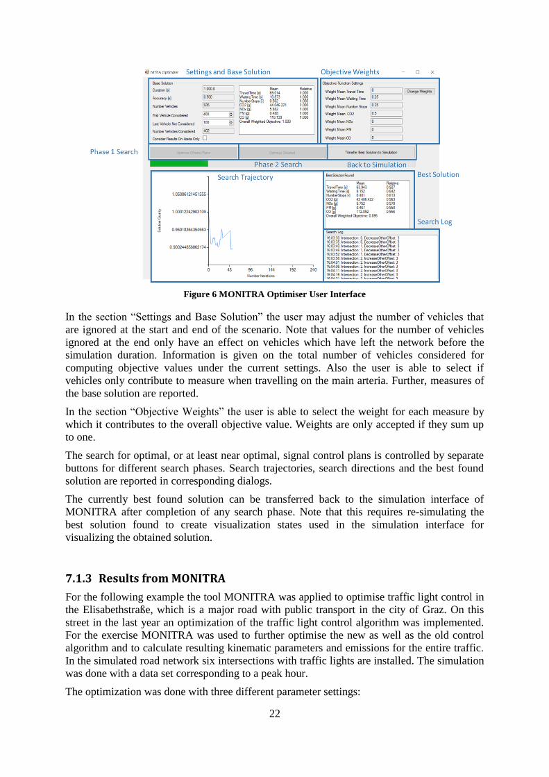
22
Figure 6 MONITRA Optimiser User Interface
In the section “Settings and Base Solution” the user may adjust the number of vehicles that
are ignored at the start and end of the scenario. Note that values for the number of vehicles
ignored at the end only have an effect on vehicles which have left the network before the
simulation duration. Information is given on the total number of vehicles considered for
computing objective values under the current settings. Also the user is able to select if
vehicles only contribute to measure when travelling on the main arteria. Further, measures of
the base solution are reported.
In the section “Objective Weights” the user is able to select the weight for each measure by
which it contributes to the overall objective value. Weights are only accepted if they sum up
to one.
The search for optimal, or at least near optimal, signal control plans is controlled by separate
buttons for different search phases. Search trajectories, search directions and the best found
solution are reported in corresponding dialogs.
The currently best found solution can be transferred back to the simulation interface of
MONITRA after completion of any search phase. Note that this requires re-simulating the
best solution found to create visualization states used in the simulation interface for
visualizing the obtained solution.
7.1.3 Results from MONITRA
For the following example the tool MONITRA was applied to optimise traffic light control in
the Elisabethstraße, which is a major road with public transport in the city of Graz. On this
street in the last year an optimization of the traffic light control algorithm was implemented.
For the exercise MONITRA was used to further optimise the new as well as the old control
algorithm and to calculate resulting kinematic parameters and emissions for the entire traffic.
In the simulated road network six intersections with traffic lights are installed. The simulation
was done with a data set corresponding to a peak hour.
The optimization was done with three different parameter settings:

23
(a) “Standard” green wave application with equal weighting of “waiting time” and
“number of stops” in the target function
(b) Extension to consider also CO2 emissions (equal weighting of “CO2”, “waiting time”
and “number of stops” in the target function)
(c) Emission optimization (only CO2 in the target function)
The optimization algorithm looks for each parameter on the reduction against the base case
and looks for an optimum of the weighted average improvement of the parameters according
to the user defined weightings.
The simulation shows that an optimization for “waiting time” and “number of stops” does not
result in the lowest emission levels (Setting a) compared to setting c) in Table 3 and Table 4.
Combining “waiting time”, “number of stops” and CO2 emissions in the target function gives
low values for all relevant parameters in this example. 100% weight for CO2 in the target
function results in increased travel time and waiting time which however are still below the
base case which represent the actual control algorithm or the algorithm applied until 2014.
Depending on the base case considered the reduction potential for emissions by optimization
given by MONITRA is in the range of 10% for emissions.
The reason for different optima in “waiting time”, “number of stops” and emissions is the
important effect of mechanical braking on overall energy consumption and emissions (see
Table 1). Negative effects of stops depend on the harshness of the braking events in front.
Longer waiting times can be overcompensated in terms of emissions if this leads to avoidance
of braking events.
Table 3: Optimisation results for Elisabethstraße with old traffic light algorithm
Travel Time
Waiting Time
Number of Stops CO2 NOx PM CO
Total speed
Driving speed
[s] [-] [g] [m/s]
Base case (1) 69.59 20.68 1.13 425737 57.0 4.71 1136 7.0 9.4
a) 58.38 11.98 0.69 397212 55.1 4.33 1034 8.2 9.8
b) 58.52 12.27 0.70 395362 55.0 4.30 1024 8.1 9.8
c) 60.52 14.68 0.80 389131 55.1 4.16 986 7.9 9.9
(1)… base case is a quite old control system which was replaced already a year ago
Table 4: Optimisation results for Elisabethstraße with new traffic light algorithm
Travel Time
Waiting Time
Number of Stops CO2 NOx PM CO
Total speed
Driving speed
[s] [-] [g] [m/s]
Base case (2) 67.17 19.59 0.92 408977 57.04 4.39 1033 7.3 9. 6
a) 54.41 8.40 0.54 393568 55.7 4.23 994 8.9 10.5
b) 54.42 8.46 0.55 392871 55.7 4.22 990 8.9 10.2
c) 57.40 11.90 0.70 384721 55.6 4.06 938 8.3 10.0
(2)… base case is an already optimised control system

24
Since the actual release version of MONITRA model was finalised at the end of COLOMBO
project yet no corresponding publications are available. For more information you can contact