NISTHB 157

Guidelines for Radiometric

Calibration of Electro-Optical Instruments for Remote Sensing

Joe Tansock, Daniel Bancroft, Jim Butler, Changyong Cao, Raju Datla, Scott Hansen, Dennis Helder, Raghu

Kacker, Harri Latvakoski, Martin Mlynczak, Tom Murdock, James

Peterson, David Pollock, Ray Russell, Deron Scott, John Seamons, Tom Stone,

Alan Thurgood, Richard Williams, Xiaoxiong (Jack) Xiong, Howard Yoon

This publication is available free of charge from: http://dx.doi.org/10.6028/NIST.HB.157

April 2015

U.S. Department of Commerce

Penny Pritzker, Secretary

National Institute of Standards and Technology Willie May, Acting Under Secretary of Commerce for Standards

and Technology and Acting Director

NIST HB 157

Guidelines for Radiometric Calibration of Electro-Optical

Instruments for Remote Sensing

Raghu Kacker Applies and Computational Mathematics Division

Information Technology Laboratory

Howard Yoon Sensor Science Division

Physical Measurement Laboratory

This publication is available free of charge from:

http://dx.doi.org/10.6028/NIST.HB.157

May 2015

U.S. Department of Commerce Penny Pritzker, Secretary

\National Institute of Standards and Technology Willie May, Acting Under Secretary of Commerce for Standards and Technology and Acting Director

i

PREFACE

This publication provides guidelines for conducting radiometric calibrations of electro-optical (EO) sensors. It is intended for use by managers, technical oversight personnel, scientists, and engineers as a reference for planning and successfully executing sensor calibrations. This document is a collaborative effort between the US government, academic institutions, and industry, and represents lessons learned from experts with years of accumulated knowledge and experience planning, reviewing, preparing, conducting, analyzing, implementing, and reporting calibration efforts.

Technical terms and definitions are introduced as needed throughout the document. Important terms, acronyms, and common references used in this text are summarized in the glossary at the end of the publication.

The manuscript contents are solely the opinions of the authors and do not constitute a statement of policy, decision, or position on behalf of NOAA or the U.S. Government. Any mention of commercial products is for information only; it does not imply recommendation or endorsement by NIST or author organizations.

ii

ACKNOWLEDGEMENTS

While this publication would not be possible without modest levels of institutional support from Space Dynamics Laboratory (SDL), National Institute of Standards and Technology (NIST), National Aeronautics and Space Administration (NASA), National Oceanic and Atmospheric Administration (NOAA), The Aerospace Corporation1, Frontier Technology, Inc. (FTI), U.S. Geological Survey (USGS), University of Alabama in Huntsville (UAH), and South Dakota State University (SDSU), it is primarily the effort of the authors who made this work possible. This is especially true of Joe Tansock, who took the lead in coordinating the efforts, making assignments, authoring specific sections, editing, and pulling it all together. The authors gratefully acknowledge the efforts of Peg Cashell at SDL for providing technical writing and editing expertise to this document.

1 This work is supported at The Aerospace Corporation by the Independent Research and Development program.

iii

CONTENTS

AUTHORS AND AFFILIATION ...................................................................................................v

EXECUTIVE SUMMARY .......................................................................................................... vii

INTRODUCTION .......................................................................................................................1

PRINCIPLES OF EFFECTIVE CALIBRATIONS ...................................................................5

2.1 Lessons Learned .................................................................................................................. 5 Calibration Planning Should Begin in the Early Stages of Sensor Design .............. 5 Trade-Offs Must be Made when Planning and Implementing a Calibration Effort . 5 Calibration Measurements Must be Traceable within a Specified Uncertainty ....... 6 System-Level Testing Provides the Best Representation of Sensor Performance ... 7 Both Pre- and Post-Launch Calibrations are Critical to a Successful Calibration ... 9

2.2 Calibration Responsivity Domains ................................................................................... 10 2.3 Calibration Requirements across Disciplines ................................................................... 11

Earth Sciences ........................................................................................................ 11 Atmospheric Sciences ............................................................................................ 13 DoD Applications ................................................................................................... 14

CALIBRATION TRACEABILITY, MEASUREMENT UNCERTAINTY, AND VERIFICATION AND VALIDATION ...................................................................................17

3.1 Traceability ....................................................................................................................... 17 Metrological Traceability ....................................................................................... 18 Metrological Traceability and Remote Sensing Measurements ............................. 19 Système International (SI) Traceability ................................................................. 20

3.2 Measurement Uncertainty ................................................................................................. 24 3.3 Verification and Validation (V&V) .................................................................................. 28

CALIBRATION PLANNING ..................................................................................................31

4.1 Early Calibration Planning ................................................................................................ 31 Calibration Planning Trade-Off Space ................................................................... 31 Detailed Test Schedule ........................................................................................... 32 Component- vs. System-Level Testing .................................................................. 33 Pre- and Post-Launch Calibration Needs ............................................................... 33 Sensor Performance Model .................................................................................... 34 Calibration Parameters and Equations ................................................................... 35 Capabilities Required for Calibration Data Collection .......................................... 37 Environmental Conditions for Pre-Launch Calibration ......................................... 41 Day in the Life Tests .............................................................................................. 42

4.2 Calibration Plans and Procedures ..................................................................................... 43 Strawman Calibration Plan ..................................................................................... 43 Comprehensive Calibration Plan ............................................................................ 44 Data Collection Procedures .................................................................................... 44 Human Resource Requirements ............................................................................. 45

4.3 Data Collection and Data Management System ............................................................... 45 Data Collection and Data Management Plan ......................................................... 45 Data Collection and Data Management Hardware ................................................. 45

iv

Data Collection and Data Management Software .................................................. 47 Automated Data Collection .................................................................................... 48 Real-Time Display and Monitoring ....................................................................... 49

PRE-LAUNCH CALIBRATION ..............................................................................................51

5.1 Preparations....................................................................................................................... 51 5.2 Engineering Testing .......................................................................................................... 51 5.3 Ground Support Equipment (GSE) ................................................................................... 52

Test Chambers ........................................................................................................ 52 Calibration Sources ................................................................................................ 53 Sensor GSE ............................................................................................................. 58 GSE Preparation ..................................................................................................... 58 GSE Operation and Traceability Maintenance ....................................................... 60

5.4 Pre-Launch Calibration Data Collection and Data Quality Assessment .......................... 61 5.5 QuickLook Analyses ......................................................................................................... 62

POST-LAUNCH CALIBRATION ...........................................................................................63

6.1 Early Operations ............................................................................................................... 63 6.2 Intensive Calibration and Validation ................................................................................ 63 6.3 Sensor Performance Trending........................................................................................... 64 6.4 On-Orbit Calibration Sources ........................................................................................... 65

On-Board Calibration Sources ............................................................................... 66 Stars ........................................................................................................................ 70 Lunar Calibration Source ....................................................................................... 73 Other Celestial Object Calibration Sources ............................................................ 78 Vicarious Calibration ............................................................................................. 79 Pseudo Invariant Calibration Sites (PICS) ............................................................. 81 On-Orbit Cross-Calibration .................................................................................... 83 Solar Diffusers ........................................................................................................ 84

6.5 Frequency of On-Orbit Calibration Measurements .......................................................... 85

DATA ANALYSIS AND REPORTING ..................................................................................87

7.1 Data Analysis Software ..................................................................................................... 87 7.2 Data Authentication .......................................................................................................... 87 7.3 Calibration Report ............................................................................................................. 87 7.4 Cross-Checks and Traceability ......................................................................................... 89 7.5 Long-Term Repository of Calibration Data ...................................................................... 90

REFERENCES ..............................................................................................................................91

COMMON EO SENSOR CALIBRATION REFERENCES ......................................................103

ACRONYM LIST ........................................................................................................................104

GLOSSARY OF TERMS ............................................................................................................107

BIOGRAPHICAL SKETCHES OF AUTHORS.........................................................................123

v

AUTHORS AND AFFILIATION (ALPHABETICAL ORDER BY AFFILIATION)

Ray Russell The Aerospace Corporation, Mail Stop M2 – 266, P.O. Box 92957 Los Angeles, CA 90009-2957 ray.w.russell@aero.org

David B. Pollock pollockd@uah.edu

Daniel Bancroft Frontier Technology, Inc. Beverly, MA dbancroft@fti-net.com

Tom Murdock Frontier Technology, Inc. Beverly, MA tmurdock@fti-net.com

Jim Butler Goddard Space Flight CenterGreenbelt, MD james.j.butler@nasa.gov

Martin Mlynczak Langley Research Center Hampton, Virginia m.g.mlynczak@nasa.gov

Xiaoxiong (Jack) Xiong Goddard Space Flight CenterGreenbelt, MD xiaoxiong.xiong-1@nasa.gov

Raghu Kacker Gaithersburg, MD raghu.kacker@nist.gov

Howard Yoon Gaithersburg, MD howard.yoon@nist.gov

Raju Datla NOAA Affiliate College Park, MD raju.datla@noaa.gov

Changyong Cao NOAA College Park, MD changyong.cao@noaa.gov

Joe Tansock 1695 Research Park Way Logan, UT 84341 joe.tansock@sdl.usu.edu

Harri Latvakoski harri.latvakoski@sdl.usu.edu

James Q. Peterson james.peterson@sdl.usu.edu

Deron Scott deron.scott@sdl.usu.edu

Scott Hansen scott.hansen@sdl.usu.edu

John Seamons john.seamons@sdl.usu.edu

Alan Thurgood alan.thurgood@sdl.usu.edu

Dennis Helder South Dakota State UniversityDennis.Helder@sdstate.edu

Tom Stone Flagstaff, AZ tstone@usgs.gov

Richard Williams Northrop Grumman Corp. Azusa, CA richard.williams@ngc.com

vi

This Page Intentionally Left Blank

vii

EXECUTIVE SUMMARY State of the art electro-optical (EO) sensors designed for today’s space-based applications require thorough, system-level radiometric calibrations to characterize the instrument and to ensure that all mission objectives are met. Calibration is the process of evaluating the parameters required to understand and describe the performance of a sensor. Through the calibration process, the sensor’s response to a radiometric input is quantified, the interactions and dependencies between the optical and electronic components are characterized and systematic errors that may result are discovered and evaluated, and traceability to national and international standards is established by rigorous calculation of the associated uncertainties. Calibration increases the probability of mission success by verifying that the sensor will meet mission requirements with a correct interpretation of the data to make accurate mission decisions.

This publication provides guidelines for conducting EO sensor calibrations. It is intended for use by managers, technical oversight personnel, scientists, and engineers as a reference for planning and successfully executing a sensor calibration.

Lessons learned from calibration experts throughout the U.S. and the world show that successful and effective calibrations have various elements in common, and that these elements should always be considered for a calibration effort. These elements include:

Calibration planning should begin in the early stages of sensor design to optimize calibration efficiency in the final design

Trade-offs between performance, cost, and schedule must be made when planning and implementing a calibration effort

Calibration measurements should be traceable with a thoroughly analyzed uncertainty

System-level testing provides the best picture of sensor performance

Both pre- and post-launch calibrations are critical to a successful calibration and traceability of the sensor data

CALIBRATION TRACEABILITY, MEASUREMENT UNCERTAINTY, AND VERIFICATION AND VALIDATION

The foundation of effective calibration is built upon national and international standards of measurement. This foundation consists of traceability, measurement uncertainty, and verification and validation (V&V), which work together to provide confidence in the sensor data output. Traceability refers to the ability to track a measurement to a known standard unit of measurement within a rigorous calculated uncertainty. V&V ensures that the instrument operates as designed and produces relevant data by proven processes and standards. All three are required to obtain reliable data that can be directly compared to model predictions and results from other instruments, among other uses.

CALIBRATION PLANNING

To be effective, calibration must be considered at all stages of a sensor program. Calibration planning for the lifetime of a sensor promotes an optimum calibration approach, reduces costs and expenditures, and minimizes uncertainty for the intended application. This planning should begin during the sensor design phase and continue until the sensor is no longer collecting data.

viii

Experienced calibration personnel must be involved throughout the lifetime of the sensor, including its development phase, to optimize calibration efforts.

The goal of calibration planning is to determine the most efficient calibration approach that meets performance requirements, while minimizing calibration uncertainty, schedule, cost, and risk. Trade-offs that must be considered during calibration planning include the test schedule, component-level vs. system-level testing, and pre-launch vs. post-launch calibration needs.

In addition to trade-off studies, a sensor performance model and uncertainty budget should be compiled to identify the parameters and characterization required to understand the sensor's performance. These tools support both system design and calibration planning, and lead to the development of sensor-specific calibration equations that are used to convert the sensor output (in units of counts, volts, etc.) to the desired scientific data products.

The calibration planning process is often initiated by first developing a strawman calibration plan that identifies the sensor, science, project, and mission requirements that are then used to determine the needed calibration parameters. Based on the strawman plan, a more mature and detailed comprehensive calibration plan is generated. Step-by-step data collection procedures are then developed to identify each step of the data collection process to ensure that the resulting data is adequate for subsequent analyses.

A data collection and management system must also be developed and tested during the calibration planning period. This involves preparing a data collection and management plan, and developing the hardware and software required for the effort. Successful data collection and management systems can control and monitor the required tasks of setting the sensor's operating state, test environment, and calibration sources to known values, verifying that the sensor’s response is within an acceptable range, and storing data for future detailed analysis tasks. A well designed data collection and management system can minimize the volume of data that needs to be collected and the time required to collect it. It can also organize collected data so that analysts have quick access to the information needed to evaluate sensor performance.

PRE-LAUNCH CALIBRATION

Execution of an effective calibration begins with pre-launch calibration measurements and continues after the sensor is placed in orbit. During pre-launch calibration, or ground calibration, tests are performed in a controlled environment with known sources that cannot be duplicated on orbit. Measurements made during pre-launch calibration are used to verify proper instrument operation, quantify calibration equation and radiometric model parameters, and estimate measurement uncertainties. Pre-launch testing provides information on sensor performance nuances that can be addressed and understood before launch. In addition, anomalies may be uncovered and resolved before launch. Options to measure unexpected behavior and implement corrections to sensor performance on orbit are often limited and expensive.

System-Level Testing and Calibration - System-level calibration can be visualized as the quality control aspect of system design and testing (Wyatt 1991). Characterizing the integrated system identifies interactions and dependencies between the optical and electronic components, and allows systematic errors to be discovered, evaluated, and resolved before flight. System-level calibration also validates the sensor model predictions and is used to determine the sensor performance uncertainty.

When conducting pre-launch calibration, it is best to follow the axiom “test like you fly” (TLYF) (Datla et al., 2011; Russell 2008), which states that instruments should be calibrated as closely as

ix

possible to the same environmental conditions expected during operation. Testing under conditions that simulate the on-orbit environment usually requires special equipment that is compatible with environmental factors such as vacuum, temperature, and contamination. Special test hardware must be used during calibration to simulate these on-orbit conditions and to present specific scenes to the unit under test. Thermal vacuum (TVAC) chambers are used to provide the mechanical, electrical, and thermal configurations required by the sensor.

Ground Support Equipment (GSE) – The quality of a calibration is only as good as the tools and references used to perform the calibration; therefore, the equipment used in the calibration, typically referred to as GSE, must be well-characterized, stable, and accurate. This process can take considerable time at a significant cost. This equipment typically includes test chambers, calibration sources, electrical support equipment (ESE), the data collection and management system, and the sensor GSE.

Ground Calibration Sources – Various calibration sources are used to provide well understood and/or repeatable flux levels as optical input to the sensor being calibrated. There are many commonly used ground calibration sources including spectral, spatial, linearity, radiance, irradiance, temporal, and scene generation sources.

Engineering Test – An engineering test is often performed prior to the start of ground calibration data collection. This test helps verify sensor operation, calibration hardware operation, data collection automation and management, and the flow of calibration test procedures and test configurations. It can also help identify additional tests that may be needed to further quantify the sensor performance. Measurements made during engineering testing can also provide preliminary data that can be used for future analyses.

Data Collection and Data Quality Assessment – During calibration testing, the data collection engineer will follow the procedure, fill in log entries, and make note of events or conditions that may affect the data. Real-time displays provide feedback to verify proper instrument configuration, GSE configuration, and response levels. Data quality checks should also be performed throughout the data collection period. Quicklook analyses of subsets of the calibration data can help evaluate data quality and can provide additional guidance to the remainder of the calibration campaign. The data quality assessment approach is unique to each payload/sensor and should be addressed in the calibration plan. The goal of data quality assessments is to obtain confidence that the data can be used for the intended calibration analyses.

Quicklook Analyses – Quicklook analyses are performed during testing shortly after data are collected for each test. These analyses provide preliminary instrument performance results, and help provide confidence that the intended, more detailed analyses (usually performed post calibration testing) can be successfully completed. These results, often presented in the form of graphs and tables in a similar format to the intended final analyses, allow project leaders to make educated path forward decisions.

Day in the Life Test – A day in the life (DITL) test may be performed pre-launch to understand the expected behavior of the sensor in its on-orbit environment, to flush out any residual concerns with how the sensor will be used on-orbit, and to implement a test-like-you-fly philosophy. This is usually performed for a full 24-hour period to attempt to mimic the diurnal variations of the expected on-orbit environment on the worst case day, and to provide the opportunity for commanding and data loading of the system to mimic what is expected during flight operations. The DITL test will help identify consequences of actual operation of the sensor that may not have been anticipated and thus may not be in the models for the sensor or the sensor plus space bus.

x

POST-LAUNCH CALIBRATION

The most effective calibration approach builds on pre-launch characterization with post-launch, or on-orbit, data collection. The goals of post-launch calibration are to verify and validate the calibration parameters determined pre-launch, characterize or update parameters that are more successfully characterized from on-orbit measurements, quantify calibration uncertainty, and update calibration coefficients if necessary to meet measurement requirements. In addition, sensor calibration must be maintained throughout mission life, and changes in sensor behavior due to component aging and/or sensor contaminations must be trended and managed.

Once the instrument reaches orbit, on-orbit calibration operations begin. These operations are used to show whether the sensor is functional and/or whether any significant changes have occurred to the sensor during launch. Specific procedures for on-orbit operations are then implemented to derive/verify parameters that were not measured during ground testing or to update those parameters that can be conducted in both ground and on-orbit operations. Sensor performance trending continues for the duration of sensor operations using on-board sources and on-orbit sources to demonstrate that measurements collected continue to meet the standards required for the sensor.

After launch, calibration measurements necessarily take second place to mission observations and must be interwoven into the mission timeline to minimize on-orbit calibration time. The decreased availability of on-orbit calibration time highlights the importance of a comprehensive pre-launch calibration. In addition, on-orbit calibration measurements typically require observation of on-orbit calibration sources that are different from the mission observation targets and therefore cannot be performed simultaneously with the mission data collections.

On-Orbit Calibration Sources – On-orbit calibration measurements are implemented using whatever observable sources may be available to serve as a calibration source, including on-board devices, sources that are ejected from the payload, celestial objects, natural or artificial sites on the surface of the Earth, and solar diffusers. In addition, sensors can view space as a zero radiance source as part of on-board calibration, and sensors can be compared to calibrated sensors in another orbit viewing the same Earth scene at the same time.

DATA ANALYSIS AND REPORTING

An unbroken process of data analysis and reporting should continue from pre-launch into post-launch calibration to capture lessons learned from pre-launch testing and maximize program efficiency. Analyzing calibration and sensor performance data requires experienced analysts and a variety of software tools that are frequently developed, or modified, from existing tools, specifically for the particular sensor program. Many if not all of these tools and algorithms are applicable to post-launch as well as pre-launch data analysis.

The results of the calibration effort are usually documented in a detailed calibration report. The overall goal of the calibration report is to provide quantitative evidence of measurement performance. This report can also be used for future reference to assist in answering critical performance/technical and pragmatic questions.

The large amounts of data often generated during calibration testing provide a lasting resource to the end user. Pre-launch test and calibration data must be archived in such a way that they are available for the analyst at all times during the pre-launch and operational phases of the mission. The lessons learned and knowledge gained from analyzing the ensemble of data from all phases of the mission can benefit the next generation of sensors.

1

INTRODUCTION State of the art, remote sensing electro-optical (EO) sensors being designed for today’s space-based applications require thorough radiometric calibrations to characterize the instrument and to ensure that all mission objectives are met. The purpose of calibrating EO sensors is to measure characteristics of a remote object, such as the Earth or celestial objects, to estimate their radiometric responsivity characteristics (emissive, reflective, and transmittance), spatial (position, size, and distribution), spectral (spectral content), temporal (changes with time), and polarization properties. These properties are inferred from the sensor’s response to the flux incident upon its entrance pupil or aperture. Success in defining object attributes using remote-sensing techniques therefore requires that the sensor response be thoroughly defined and understood, which can only be accomplished by EO sensor radiometric calibration. (Wyatt 1991).

The calibration guidelines provided in this document begin with the early stages of the sensor design and address calibration throughout the life-cycle of the sensor. The following chart maps the publication contents into a notional, but often typical, sensor life-cycle time line, covering sensor preliminary design to post-launch operations.

2

What is EO Sensor Radiometric Calibration for Remote Sensing? Calibration is the process of characterizing the parameters required to understand and quantify the performance of a sensor for its intended application. This calibration process also converts a sensor’s output (in units of counts, volts, etc.) to physical units (often radiometric units such as W/cm2, J/sec/cm2, etc.) with traceability to a known standard and within a specified uncertainty.

Why is EO Sensor Radiometric Calibration Necessary? EO sensors require calibration to quantify the sensor’s response to known radiometric input and to characterize the interactions and dependencies between the optical, mechanical, and electronic components. In addition, sensor specific performance dependencies and systematic errors can be identified through calibration.

Calibration increases the probability of mission success by:

Identifying measurement performance and limitations Providing characteristic equations and parameters that relate the measured signal to the

true scene radiance and spatial content Allowing timely and correct interpretation of data to make more accurate mission

decisions Minimizing the impact of sensor behavior on the intended measurements by identifying

and characterizing unique sensor performance characteristics Quantifying measurement uncertainty that can be used to provide a clear understanding

of the data Verifying that the sensor will meet mission requirements

Sensor calibration affects the quality of the interpretation of the data, and thus the success or failure of the performance of the critical task, not just the success or failure of a particular sensor or program. This applies to both science and Department of Defense (DoD) remote sensing applications.

The following examples highlight sensor missions that owe their success in part to a thorough calibration. Subsequent sections in this document provide a complete overview of EO sensor calibration and the sensor performance obstacles that can be minimized by proper attention to calibration in remote sensing work.

Calibration efforts contributed to the success of Landsat.

Connecticut River after Hurricane Irene

(Sensor: L5 TM, Acquisition Date: 9/2/11) (USGS/NASA Landsat)

3

Landsat

The Landsat program, which has provided the longest-running continuous data set of high spatial resolution Earth imagery, attributes its success partly to the ability to understand the radiometric properties of the sensors due to the combination of pre-launch and post-launch calibration efforts (Thome et al., 1997). Over 15,000 coefficients are issued to span distinct timeframes and are continually updated with improved calibration coefficients. The radiometric calibration of these systems allows the full Landsat data set to be used in a quantitative sense.

SABER

http://saber.gats-inc.com

The Sounding of the Atmosphere using Broadband Emission Radiometry (SABER) instrument is a 10-channel radiometer that spans the range of wavelengths from 1.27 µm to 17 µm. The instrument uses state-of-the-art mechanical cooling of the detector focal plane array to 75 K to achieve high radiometric sensitivity, operational flexibility, and long experiment life. An in-flight calibration system is incorporated to provide high long-term accuracy (Russell et al., 1999). SABER was launched in 2001 on the NASA Thermosphere-Ionosphere-Mesosphere Energetics and Dynamics (TIMED) satellite to study the structure, composition, and energy balance in the Earth’s mesosphere and lower thermosphere (Mlynczak 1997). The instrument is still obtaining data in 2014. An accurate calibration and detailed instrument characterization of the SABER instrument were fundamental to the ability of SABER to generate meaningful geophysical data products. The ground calibration of this instrument is described by Tansock et al. (2003) and a calibration update in Tansock et al. (2006).

CERES

http://www.nasa.gov/mission_pages/NPP/news/cer

es-on-npp.html

The Clouds and the Earth’s Radiant Energy System (CERES) instruments on the NASA Terra, Aqua, and Suomi/NPP spacecrafts (Wielicki et al., 1996) are examples of instruments used to measure the Earth’s climate system. The CERES instruments are highly accurate, broadband radiometers that measure top-of-atmosphere (TOA) fluxes of the reflected solar irradiance and the emitted infrared irradiance. TOA net radiation is the long-term global average of the incoming and outgoing energy from the Earth. In an equilibrium climate state this difference is zero. If the climate is forced, there is an imbalance in the TOA irradiances as the Earth works to restore balance. This imbalance may be on the order of ~ 1 W/m2, which is hard to detect. Many instrument issues can cause changes in the instrument calibration over time, and unless accounted for, will appear as changes in the climate system. Therefore, a thorough understanding of the sensor system is required for accurate climate measurements.

SPIRIT III

http://space.skyrocket.de/

doc_sdat/msx.htm

The Spatial Infrared Imaging Telescope (SPIRIT III) was launched aboard the Mid-course Space Experiment (MSX) spacecraft on 24 April 1996. To assure accuracy and instill confidence in the data, the project developed methodologies to certify the process of converting raw sensor data to calibration corrected output. For this project, the raw data along with the tools needed to apply calibration were archived, allowing the user to reprocess data as calibration was refined. Data quality was verified by the Performance Assessment Team (PAT) and the entire process was reviewed by the Data Certification and Technology Transfer (DCATT) committee and included end-to-end certification testing and uncertainty evaluation. A detailed and comprehensive calibration approach was implemented (both ground and on-orbit making use of all available external and internal on-board calibration sources with an emphasis on traceability). Repeatability was achieved by controlling the configuration of the sensor, data processing software, calibration software, and calibration parameters. This rigorous approach provided a common starting point from which the several principle investigator teams were able to proceed with confidence. The final MSX report is documented in MSX Data Application for Future MDA Overhead Persistent Infrared (OPIR) Efforts (SDL/09-576B). Publications associated with the MSX program are archived in MSX Bibliography, Version 3.3.2, Cleared for Public Release, SRE Log #0006-2601 and BMDO Case 00-S-2657 (U) https://dcp.mda.mil/

4

What is the Future of Calibration? Accurate calibration is becoming increasingly important for sensors. Calibration to achieve relative uncertainty of less than 1 % of the measured radiance is essential for the accurate retrieval of atmospheric temperature. Recognizing that absolute calibration is the limiting factor to detecting climate change from measurements made by orbiting satellites, industry leaders have proposed new approaches to calibration to achieve the required performance. One such proposal is the Climate Absolute Radiance and Refractivity Observatory (CLARREO) instrument (discussed in the following example), which represents the pinnacle of calibration and instrument characterization. The on-orbit ability to trace measurements to Système International (SI) units and to detect instrument changes for the life of the mission will produce a data set that researchers can use for decades, or return to decades later, with complete understanding of the data set, its measurement uncertainty, and its implications for the climate.

CLARREO The NASA Climate Absolute Radiance and Refractivity Observatory (CLARREO)

mission was recommended by the National Academy of Science in 2007 (NRC 2007) as an innovative mission focused on detecting and attributing climate change from space-based measurements of Earth’s infrared and visible radiance spectra. The hallmark of CLARREO is its ability to tie radiance measurements, on orbit, to known metrological standards through the international system of units (Système International (SI) units).

CLARREO is unique in that it will monitor absolute calibration and key instrument performance parameters, on orbit, for the life of the mission. The sensor will carry devices such as infrared lasers to monitor emissivity changes during the life of the mission, so that even these seemingly small instrument changes will not mistakenly be interpreted as changes in the climate system. Absolute radiometric accuracy will be maintained by calibration of every measured spectrum, and traceability of those spectra will be to the kelvin temperature standard through reference to a blackbody of known temperature, on orbit, for the life of the mission. The CLARREO mission is described in detail in Wielicki et al. (2013), and the concepts behind the infrared instrument on CLARREO are outlined by Anderson et al. (2004). As of late 2014, the CLARREO mission remains in pre-formulation status within NASA.

The CLARREO mission benchmark measurements can provide calibrations to other satellite sensors through inter-comparison using the simultaneous nadir overpass (SNO) observations described in Section 6.4.7. NOAA researchers showed the SNO technique to be an effective way to intercompare satellite observations when the satellites cross in their orbits at the same time and make nadir observations of the Earth simultaneously (Cao and Heidinger 2002).

5

PRINCIPLES OF EFFECTIVE CALIBRATIONS Calibration is becoming increasingly more challenging as measurement requirements become more stringent, particularly in climate change applications. Scientists, engineers, and managers involved with calibration efforts often exchange information through conferences and publications to discuss and learn from past and present calibration efforts, with the goal of improving calibration (Tansock et al., 2006). Lessons learned from these discussions show that successful and effective calibrations have various elements in common and that these elements should always be considered when planning a calibration effort.

2.1 LESSONS LEARNED

Calibration Planning Should Begin in the Early Stages of Sensor Design

Calibration is critical to the success of a mission. Unfortunately, it is often an afterthought in the development of the sensor. This lack of planning can lead to increased testing times and inaccurate results. Early calibration planning throughout the lifetime of the program promotes an optimum sensor calibration approach that reduces costs and expenditures while minimizing uncertainty for the intended application. Experienced calibration personnel must be involved throughout the sensor’s development phase to optimize calibration efforts.

A thorough system-level calibration approach should begin in the early stages of the sensor design and address calibration throughout the lifetime of the sensor (Tansock et al., 2004), including component- and system-level calibration, spacecraft integration and test, and on-orbit operations. Delaying calibration planning can lead to limited options for the calibration approach and can often be more expensive to execute.

Calibration planning should begin during the preliminary sensor design phase to ensure the instrument is designed to facilitate calibration. After the sensor design has passed the critical design phase, an end-to-end calibration plan should be developed to ensure that the calibration approach meets sensor performance requirements. Data management and analysis needs must be considered due to the large amounts of data produced by many of today’s sensors.

Trade-Offs Must be Made when Planning and Implementing a Calibration Effort

Sensor programs have limited funding, resulting in trade-offs in costs, phasing of available funds, and scope of calibration. There is always a trade-off between what is ideal, what is desired, and what is strictly required when performing sensor calibration. While it may seem expedient at the time, reducing the scope of the calibration effort to reduce costs may in fact lead to more costly issues later in the program that impact the success of the mission. The axiom “You only have one opportunity to collect the data” is for the most part true. Therefore, knowledgeable experts who

Lessons learned provide guidance for successful sensor calibration.

6

can identify trade-offs among available budget, schedule, and impact to sensor performance or mission objectives should be included when deciding on test program specifics.

Sufficient calibration data must be collected to span the operational envelope of the sensor, but the scope should not extend to the point where extrapolation beyond the bounds of the calibration data set is required. Attention and priority should be given to obtaining quality calibration measurements.

Investment in appropriate special test equipment and calibration sources should be budgeted and considered as a necessity. The quality of the test setup needs to be at least as good as the sensor under test (SUT) (otherwise the sensor could end up being used to calibrate the special test equipment). In addition, it may be advantageous for a program to procure spares of key components for future evaluation to help explain unexpected behavior, or even a duplicate of the integrated sensor to exercise pre-launch calibration test activities, which could reduce the risk of damaging flight hardware. This approach would provide a better understanding of the sensor performance and identify and resolve calibration issues.

Steps should be taken to optimize the calibration effort. Time can be saved by appropriate sequencing of the various tests to make the best use of analysts and resources. Optimization efforts should be assessed by a knowledgeable expert, as decisions need to be made about which specific data sets should be collected and how much data to collect. The focus of any optimization effort should be to address the issue of performing the overall sensor calibration more efficiently, and not on reducing the scope of the calibration effort. Reducing the scope of pre-launch calibration efforts may impart additional requirements for post-launch calibration, where options for collecting particular data sets are either limited or unavailable.

Calibration Measurements Must be Traceable within a Specified Uncertainty

To optimize the success of a remote sensing mission, the sensor must provide measurements that can be trusted. For example, an Earth climate science satellite’s remote sensing mission provides continuous coverage and has the potential to allow observation of climate variables through long-time periods. Climate modelers require continuous data over long time periods to test their models and predict global climate variability. These measurements must be trusted and absolute, the measurement uncertainties well understood, and the measurements must be consistent with mission expectations to be of value to the modelers. Three properties that work together to provide confidence in the sensor data are traceability, measurement uncertainty, and verification and validation (V&V).

Traceability refers to the ability to track a measurement to a known standard unit of measurement within a given measurement uncertainty. V&V ensures that the instrument operates as designed and produces relevant data by proven processes and standards. All three are required to obtain reliable data that can be directly compared to model predictions and results from other instruments.

Traceability can be achieved by using the SI-based standards of a national measurement institute, such as the U.S. National Institute of Standards and Technology (NIST). During calibration, measurements should be compared to known reference standards, and discrepancies recorded to estimate the uncertainty of the calibration. The specified uncertainty of the standard itself is a crucial component of this estimation. A calibration will typically include a traceability chain to a primary standard and a quoted overall uncertainty for the performance of the unit under test.

7

The calibration data products and sensor performance knowledge obtained during calibration play a critical role in V&V at both the sensor and the mission level, creating a critical link between sensor calibration and overall mission-level success. Sensor calibration quantifies the as-built sensor performance, providing a basis for V&V of design requirements and sensor performance in support of mission objectives.Ensuring that calibration measurements are traceable within the expected uncertainty will provide V&V that the data can be used across disciplines such as Earth sciences, atmospheric sciences, and DoD applications.

System-Level Testing Provides the Best Representation of Sensor Performance

Pre-launch calibration testing includes component-level testing and system-level testing of the completed sensor. Component-level testing is performed early during the assembly period, and provides a first look at the potential characteristics of a sensor. This testing also assists in developing model parameters used to estimate system performance. Component-level testing may help reduce costs and schedule by identifying problems at the lowest level of assembly. Component-level testing is usually not adequate to represent a full system-level calibration parameter, however.

Issues with the focus of Hubble Space Telescope illustrate the importance of pre-launch, system-level calibration (see following example). For a complete system-level calibration, sufficient measurements must be made on the fully integrated sensor to cover every design configuration of the system, the sensor’s entire dynamic range, and all expected environmental conditions. Ideally, these performance metrics can be quantified completely during system-level calibration.

System-level calibration can be visualized as the quality control aspect of system design and testing (Wyatt 1991). The advantage of system-level measurements is that all components are included in the measurement in the way they are used, as opposed to component-level measurements where differences in optical configuration, temperature, or orientation may be unavoidable.

Characterizing the integrated system identifies interactions and dependencies between the optical and electronic components, and allows systematic errors to be discovered, evaluated, and resolved before flight. Although EO sensors may be designed and manufactured to strict specifications, components may behave differently than expected once installed in an instrument, and the interactions among integrated components makes each sensor unique. The most well thought-out designs and advanced fabrication techniques can still result in system-level sensor performance that differs from design specifications.

Other factors that may contribute toward system-level performance variability include errors from the fabrication processes, changes in the components over time, and an unanticipated instrument behavior not covered by specifications.

When schedule and cost constraints indicate that component-level measurements, which generally provide a cost advantage compared to system-level measurements, must suffice for some calibration parameters, careful consideration of the trade-off between component-level convenience and system-level accuracy is mandatory. The calibration results from the SABER and

System-Level Testing System-level measurements provide confidence that details buried deep in the sensor design are fully tested. As an example, a sensor had spectral filters installed in filter wheel positions that did not match the documented positions. Had this anomaly not been identified as part of sensor-level verification performed during pre-launch calibration, confusion in the sensor data could have created credibility problems, jeopardizing the mission objectives.

8

SPIRIT III instruments, shown in the following examples, highlight the importance of performing system-level testing. The SABER instrument showed good agreement for 8 of the 10 bands, but for one of the bands, there was a difference of greater than 20 % when comparing component-level and system-level measurements. For the SPIRIT III instrument, sensor performance was compromised by an out-of-band leak that, if not discovered during system-level testing, would have limited the value of the data produced by the sensor.

When component-level measurements are used to estimate system-level calibration for a sensor, the likely increase in uncertainty and the risk of errors greater than 20 % must be recognized and deemed acceptable. A minimum amount of system-level measurements should always be planned to verify the component-level measurements.

Hubble Space Telescope

A famous example of the importance of pre-launch, system-level calibration is the focus of the Hubble Space Telescope. Component-level testing of the primary telescope mirror was performed using custom equipment, and suggested that the optics were properly manufactured. No optical performance tests were made at higher levels of assembly. However, during on-orbit checkouts, it was discovered that the telescope could not be correctly focused because of a flaw in the optics (NASA-TM-103443, November 1990). This failure was traced to flaws in the custom equipment used for component-level manufacturing and testing, and the fact that complete reliance was placed on using a single test to verify the system. It is likely that this anomaly would have been identified during pre-launch system-level calibration, potentially saving millions of program dollars.

SABER Component Measurements

Courtesy of

NASA

An example of the trade-off between component level versus system level measurements is presented in “Component Level Prediction versus System Level Measurement of SABER Relative Spectral Response” (Hansen et al., 2003), where differences between component-level and system-level measurements of the bandwidth of 10 bands in the SABER instrument were compared. In this analysis, the bandwidths measured at the component level and system level for eight of the SABER bands were consistent within 3.3 %. However, the remaining two bands showed greater differences: one showed a difference of 4.5 % between component- and system-level measurements, and one showed a difference of 23.5 %. For the bands showing large discrepancies between component-level and system-level measurements, accurate end-to-end spectral measurements were essential to achieve correct understanding of the instrument science data.

SPIRIT III Out-of-Band Leakage

During SPIRIT III engineering calibration, a significant out-of-band spectral leak caused by the Stierwalt effect was discovered (Fuqua et al., 2003). This issue was resolved by adding a sapphire blocking filter into the sensor configuration (SDL/98-033). Had this problem not been resolved, the measurement uncertainty would have been unacceptably large to accommodate this non-ideal sensor performance issue, limiting the value of the data produced by the sensor.

9

Both Pre- and Post-Launch Calibrations are Critical to a Successful Calibration

EO sensor calibration usually involves both a pre-launch and a post-launch segment. Understanding a sensor’s properties and its changes after launch is essential to generating high quality data products. Instrument issues such as optics degradation due to long-term exposure to ultraviolet (UV) radiation can cause changes in the instrument calibration over time. Unless accounted for, these changes will falsely appear as changes in the object being measured. Errors as small as several nanometers in spectral position knowledge due to improper or incomplete characterization of in-band or out-of-band contributions to the integrated sensor signal have been known to bias cloud height science products (Mlynczak et al., 2013).

Pre-launch calibration, or ground calibration, provides the capability to perform tests in a controlled environment with known sources that cannot be duplicated on-orbit, and has the advantage of discovering and resolving anomalies prior to launch. Measurements made during pre-launch calibration are used to verify proper instrument operation, to quantify calibration equation and radiometric model parameters, and to estimate measurement uncertainties. Pre-launch calibration is essential to understanding sensor performance nuances so that they can be addressed and understood before launch. Options to correct unexpected sensor performance anomalies after launch are limited and expensive.

Post-launch testing, or on-orbit calibration, has the advantage of being performed under true flight conditions rather than simulated flight-like conditions. The goals of post-launch calibration are to measure parameters that cannot be measured on the ground, maintain calibration throughout a sensor’s operational lifetime, quantify calibration uncertainty, and update calibration coefficients if necessary to meet measurement requirements.

However, on-orbit time that is dedicated to calibration is limited (Tansock et al., 2004). It is usually impractical to perform all of the on-orbit measurement combinations needed to fully calibrate and understand the sensor. A complete and sufficiently bounded pre-launch calibration will minimize the satellite operational time required for post-launch calibration.

While every effort should be made to measure and verify system parameters during pre-launch calibration, there are some parameters for which on-orbit sources may enable a better measurement, including pointing and geometrical parameters such as point response function (PRF), distortion mapping, pixel instantaneous field of view (IFOV), and off-axis scatter, where stars can provide ideal point sources, the Moon can provide a bright large area source, and ground test sites can provide uniform and spatial calibration targets. Even though on-orbit data for these

Obtaining Accurate Ocean Color Measurements

For ocean color, an accuracy of about 0.5 % is needed for TOA radiance retrieval. To achieve this level of accuracy, the contributions of artifacts such as polarization, straylight, and non-linearity need to be on the order of 0.1 %. Most of these effects can only be characterized pre-launch. However, the sensor radiometric gain is often derived on-orbit. Therefore, both pre-launch characterization and on-orbit calibration are critically important for ocean color remote sensing.

The Bering Strait (MODIS, 7/8/10)

http://oceancolor.gsfc.nasa.gov/cgi/image_ archive.cgi?c=COASTAL

10

parameters may provide a better result, prudence dictates that the best possible pre-launch measurements should be performed to verify and validate system performance and identify design and assembly “gotchas” before launch.

2.2 CALIBRATION RESPONSIVITY DOMAINS

Sensor performance is dependent on relationships between multiple responsivity domains. For characterizing EO systems, five domains should be considered: radiometric, spatial, spectral, temporal, and polarization. The goal of calibration is to characterize each of these responsivity domains independently. In an idealized setting, there would be no interactions between parameters and each responsivity domain could be characterized independently. In reality, there are interactions and much of the work of calibration goes to understanding and minimizing these interactions. Calibration planning during the sensor design phase helps to ensure that the design is compatible with the planned calibration measurements. (Hansen et al., 2011; Tansock et al., 2004).

The radiometric responsivity domain describes the sensor’s response to electro-magnetic radiant energy. Calibration parameters that describe the radiometric response of a sensor include radiance and/or irradiance calibration coefficients, response linearity, array detector-to-detector response uniformity, nominal and outlying detector identification, and radiometric calibration of internal calibration sources. Knowledge of a sensor’s radiometric domain is key to understanding how well the sensor responds on an absolute and/or relative scale. Determining the absolute radiance responsivity provides an understanding of the measurement physics of the sensor, and is necessary for a complete calibration (Wyatt 1978; Tansock et al., 2004). Absolute radiance measurements are used to verify that specifications have been achieved relative to an internationally recognized standard and to assess spectral purity (Wyatt 1978).

The spatial domain describes how measurements are affected by an object being located at a different spot in the sensor’s field of view. It includes the position of the detector with respect to the instrument boresight, the detector’s effective field of view (EFOV), and the detector’s scatter due to optical scatter and electrical crosstalk. These measurements enable experimenters to point the detectors at a desired source and to model detector responses to objects that are inside and outside the detector’s direct line of sight (Wyatt 1991).

The spectral domain measures the sensor’s response to radiation as a function of wavelength, and describes how the sensor responds to sources of different wavelengths. It is characterized by the sensor spectral response or the relative spectral response (RSR) parameter, which measures the normalized sensor response both in and out of the intended bandpass of the sensor. Knowledge of a sensor’s spectral domain provides an understanding of the sensor’s response to various spectral sources, leading to an absolute calibration for the sensor.

The temporal domain describes the sensor’s response to a well characterized, stable source throughout the mission life, including both pre- and post-launch operations. The temporal domain measurements consists of sensor repeatability for a specified time period (i.e., short, medium, and/or long) and amplitude response as a function of optical input temporal frequency. Understanding the sensor temporal frequency response is particularly important when the source being measured by the sensor has a time-varying radiometric component.

The polarization domain describes the sensitivity of the sensor to polarized light. This domain becomes important when the sensor design induces polarization sensitivity and the mission targets and/or backgrounds contain polarized light.

11

2.3 CALIBRATION REQUIREMENTS ACROSS DISCIPLINES

Sensor calibration requirements vary with the application of the sensor. The parameters to be measured during calibration are highly dependent on the instrument and the mission. Parameters that are important for one instrument may be irrelevant for another. For example, sensors for Earth and atmospheric science applications may be affected by atmospheric effects; thus, the sensor must be characterized for properties such as polarization and spectral responses to account for atmosphere polarization or spectral emission effects. For DoD applications that frequently observe above the horizon of the earth, optical performance parameters such as off-axis rejection or image quality characterizations that impact point source resolution may be more important. This section discusses calibration considerations for these different applications.

Sensors for Earth and atmospheric science applications, as well as DoD applications, generally use passive remote sensing techniques rather than active techniques involving radars or lasers/lidars.

Earth Sciences

Earth-observing sensors are designed for a broad range of studies of the Earth's land, ocean, and atmosphere, and are based on the needs of the science and user community to either enhance existing sensor data records or to advance new science and research applications. The Moderate Resolution Imaging Spectroradiometer (MODIS) and the Visible Infrared Imager Radiometer Suite (VIIRS) are examples of Earth-observing sensors that measure the Earth's radiance in a wide spectral range, and the Sea-viewing Wide Field-of-view Sensor (SeaWiFS) is an example of a sensor that measures ocean color.

For ocean color, measurement uncertainty of about 0.5 % is needed for top of atmosphere (TOA) radiance retrieval. To achieve this level of accuracy, the uncertainty contributions of artifacts such as polarization, straylight, and non-linearity need to be on the order of 0.1 %, and both pre- and post-launch calibration are required to achieve this accuracy.

The calibration requirements for Earth-observing sensors vary depending on the specific sensor application. Some observations, such as changes in the Earth’s surface properties are often determined using data from multiple sensors, which requires that the spectral characteristics and traceability of the sensors be thoroughly understood to permit accurate cross-comparison of data. These sensors must be consistently calibrated with the same traceability, ideally with the same calibration sources and techniques.

12

Calibration Traceability using Data from Multiple Sensors

The same solar diffuser design was used to maintain calibration traceability for the MODIS instruments on both the NASA Terra and Aqua Earth Observing System (EOS) satellites, as well as the S-NPP/JPSS VIIRS reflective solar bands.

(Courtesy of NASA)

A key element addressing the consistency of merged data quality is sensor spatial/spectral performance in the form of band-to-band pointing alignment, as many of the science products are spatially geolocated but are generated using more than one spectral band.

For land remote sensing, the data must be corrected for atmospheric effects, which requires well calibrated and characterized sensor properties such as polarization sensitivity and spectral responses. Otherwise, the derived products could be biased. Most land studies monitor changes in the surface properties, and the measurement products derived from these properties are very sensitive to changes in the sensor’s calibration. For example, drought monitoring relies on looking at yearly changes in vegetation using a baseline that typically contains over 10 years of data (e.g., the Normalized Difference Vegetation Index (NDVI)); undetected changes in the sensor’s calibration could be incorrectly interpreted as vegetation stress or drought (Wang et al., 2012).

13

Atmospheric Sciences

Atmospheric science EO sensors use passive remote sensing techniques to measure radiance emitted by the Earth and atmosphere, or radiance from the Sun that is reflected by the Earth and the atmosphere.

Analysis of radiance measurements generally falls into two categories: analysis for the purpose of deriving atmospheric state profiles of temperature and minor constituents (atmospheric sounding), and analysis for deriving properties related to the energy balance of the Earth system. Profiling involves retrieving atmospheric structure that is consistent with the measured radiance while requiring retrieved temperature and constituent abundances that are physically realistic. The process of “inverting” the radiative transfer equation to solve for the atmospheric structure may be highly non-linear and small, often subtle errors or uncertainties in the measured radiance (or other instrument characterization uncertainties), may render the retrieved profile useless, or at least, non-physical. Applications of measured radiance to Earth’s energy balance often do not involve non-linear radiative transfer but nonetheless depend critically on knowing absolute calibration and its time variation.

Spectral radiance is measured by Fourier transform (W/(m2·sr·cm-1)) or grating spectrometers (W/(m2·sr µm)). Spectrally integrated radiance (W/(m2·sr)) is measured by narrow-band and broadband radiometers. Some of these instruments observe in the nadir (including those that scan cross-track) for the purpose of deriving properties at Earth’s surface, in the troposphere, and in the lower stratosphere. Other instruments observe the Earth’s limb for deriving the composition and structure of the stratosphere, mesosphere, and thermosphere.

Accurate radiometric calibration and instrument characterization are essential for generating high quality data products from instruments used to remotely sense the atmosphere. Atmospheric properties such as water vapor content, cloud coverage, cloud and aerosol optical depth, cloud height, and cloud particle size and phase impact the Earth’s radiation budget. These products are generated using spectral bands in both reflective solar and thermal emissive regions. The quality of the data products relies on the spectral band radiometric bias and precision, which in turn rely on accurate characterization of sensor on-board radiometric sources and optical elements both in pre-launch and on-orbit phases of the sensor lifetime.

Passive Sensor System

Passive remote sensing techniques rely on natural radiation emitted or reflected by an object or area of interest. As shown

in the following illustration, the land (or sea) feature is illuminated by the sun, providing energy for reflected/emitted

radiance that is then measured by the remote sensing system. The measurement data are then transmitted to the

ground station for data processing and science analysis.

14

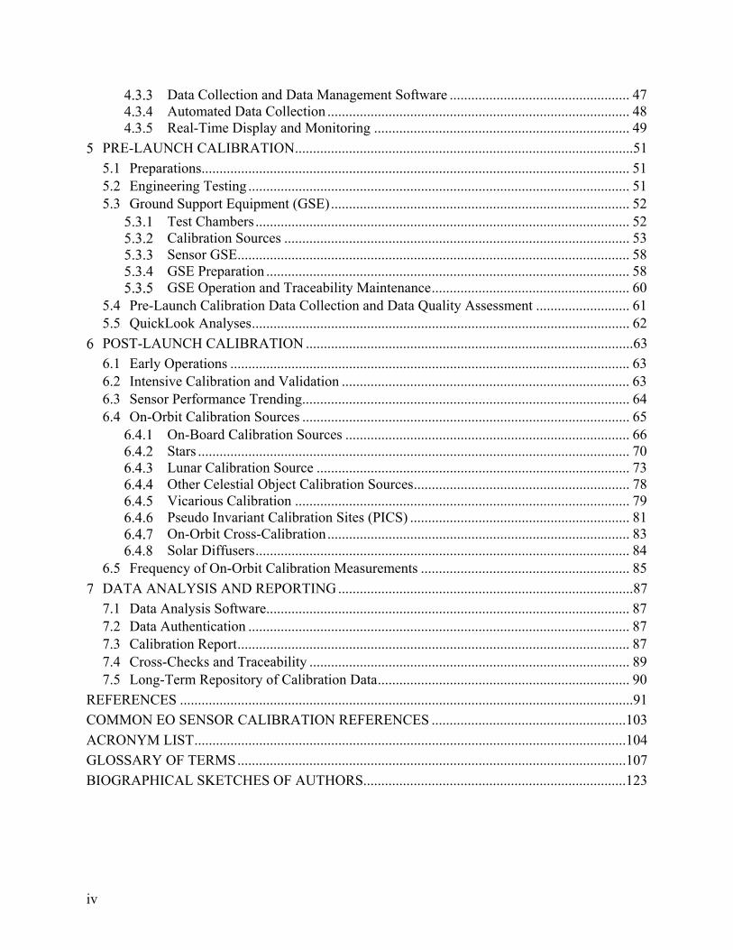
Calibration to achieve relative uncertainty of less than 1 % of the measured radiance is essential for the accurate retrieval of atmospheric temperature. The science requirement is for atmospheric temperatures to be measured with uncertainty less than 1 K. Infrared radiometers and infrared spectrometers determine temperature by measuring radiance in the carbon dioxide (CO2) bands near 15 µm (667 cm-1). The 1 K uncertainty in the Planck function (due to its sensitivity to temperature) results in uncertainty in the radiance ranging from 1.36 % at 270 K to 2.2 % at 210 K). Given that the sum of all error sources must be less than 1 K, it is clear that the relative uncertainty of the absolute radiometric calibration must be less than 1 % over the range of radiances to be observed.

DoD Applications

The DoD uses many types of sensors in multiple constellations of satellites, on drones and aircraft, and on the ground for a variety of applications. These applications include weather characterization in support of the warfighter, battle-space characterization, monitoring of missile launches (missile warning) world-wide, theater missile warning (in support of the warfighter), and for technical intelligence (TI). TI can span a large range of applications, including assessing the movement of resources for political situations, and

ascertaining the capabilities of an industrial area, such as how many missiles or vehicles are being produced in a given plant.

In addition, data from existing DoD systems are used in the architecture studies for future systems. These architecture studies rely on existing data to establish the requirements for sensitivity, spatial resolution, timeliness, spectral capability (filter bandpass locations and widths), absolute accuracy, and repeatability (precision). The expected or predicted quality of the data will also play a key role in establishing the number of sensors required for future missions, a fundamental property of the system that will be a major acquisition cost and schedule driver. For all of these applications, the calibration of the sensors will affect the quality of the interpretation of the data, and thus the success or failure of the performance of the critical task, not just the success or failure of a particular sensor or program.

Atmospheric Altitude vs. Temperature

http://saberoutreach.hamptonu.edu/overview.

html (Chart by R. Bradley Pierce, NASA LaRC)

15

In some cases, multiple DoD sensors will be used for the same purpose, such as using different constellations of sensors to perform missile warning functions. Missile warning includes not only the simple detection of a launch, but also missile typing, launch point calculation, and impact point prediction, tasks that require a collection of missile trajectories and intensity profiles. This information ultimately comes from the data obtained over many years of observing multiple launches, and is used both as empirical evidence of the behavior of a class or type of missile and to validate the models for the properties of each type of missile. An issue that arises when multiple sensors, sensor types, and constellations are used for a common application is that if the calibrations of the various instruments are based on a different set of standards, the resulting data will represent the signatures on a different scale.

Ultimately, National Metrology Institutes (NMIs), such as NIST in the USA, provides the absolute reference (“truth”) for radiometric intensity calibrations through sources or transfer radiometers. However, even with NIST-traceable sources, other issues exist. The algorithms that extract the information on a point target or provide calibrated intensities in a radiometrically calibrated scene can affect the intensities reported. In addition, when different programs with different sensors use different approaches to extracting information, the result may be a disarray of apparently conflicting information. For example, if the heat given off by a small power plant or factory is extracted from a complex urban scene, the manner used to perform the extraction can affect the values reported. If an image enhancement technique that does not preserve the energy in the scene is used, the result that is derived can be incorrect. Therefore, when results from different programs are compared, the findings may appear to be contradictory or in conflict. With the correct calibration of not only the sensors’ responses, but also of the impact of the algorithms used to perform the task, the results can come into agreement. Data fusion can then focus on the content of the data to address a problem at hand instead of a debate about why the different programs are obtaining apparently conflicting or contradictory results. The following example illustrates the importance of calibration in a DoD application.

Plume Signature Models

In the early 1980s, the intensity of missile plumes and the models for missile plumes were significantly different. It now appears that at least part of the discrepancy can be traced to an error in the absolute calibration of a constellation of space-based sensors. Currently, the models and data are in very good agreement, which has improved the ability to predict the geometrical behavior of the plume emission, the interaction of the plume signature with the atmosphere (the portion of the plume radiation that will be transmitted to the sensor along a given line of sight), and to more quickly develop an accurate model for a new missile.

16

DoD Application The measurement geometry of the MSX satellite viewing a re-entry vehicle through the Earth

limb. All aspects of calibration, including atmospheric effects, need to be applied in this scenario to accurately measure and identify the target. Information obtained from calibration is used in the calibration equation to put results on an absolute scale. Measurement results can then be compared with those of other instruments to lower uncertainty and increase accuracy of the knowledge about the target.

Reprinted with permission ©The Johns Hopkins University Applied Physics Laboratory

When performing calibrations and deriving calibration products, the environment in which the sensor is being tested needs to be representative of that which the sensor will experience during use. This “test as you fly” axiom (Datla et al., 2011; Russell, 2008) implies that instruments should be calibrated under the same environmental conditions as expected during operation. Similarly, the calibration sources, targets, and methodologies will need to be representative of the applications. If a modulation transfer function or point response function will be used for target extraction, the calibration data should be obtained in the same manner as expected during operation, using targets or scenes that are representative of those that will be studied in the real world. If signatures will be measured after transmission through the atmosphere, the RSR must be accurately characterized so that the calculations of atmospheric transmission effects will be included correctly.

When the “test as you fly” approach is used for all the sensors involved, even though they are from different programs and have had varied approaches to calibration used in their manufacture, a coherent, consistent picture of the results can be obtained. This has been demonstrated with two recently launched sensors that have dramatically different filter shapes at nominally the same wavelengths. In spite of this, the proper application of the measured and modeled RSRs for the two different systems results in consistent target intensity reports.

17

CALIBRATION TRACEABILITY, MEASUREMENT UNCERTAINTY, AND VERIFICATION AND VALIDATION As previously described (Section 2.1.3), traceability, measurement uncertainty, and V&V work together to provide confidence in the sensor data. Traceability refers to the ability to track a measurement to a known standard unit of measurement within a given measurement uncertainty. V&V ensures that the instrument operates as designed and produces relevant data by proven processes and standards. All three are required to obtain reliable data that can be directly compared to model predictions and results from other instruments. This section further discusses these properties.

3.1 TRACEABILITY

Traceability can be defined as an unbroken record of documentation or an unbroken chain of measurements, and their associated uncertainties (www.nist.gov). The principle benefits of traceability for EO sensor calibration are to improve the likelihood that data products provide a quantitative description of the measured parameter, are invariant with time, and are sufficiently robust for regulator, policy, or commercial decisions (Fox, 2004).

The definition of traceability as it applies to remote sensing has evolved over the years. In 2008, the International Vocabulary of Metrology – Basic and General Concepts and Associated Terms (VIM) reworded the term ‘traceability’ to ‘metrological traceability’, and defined it explicitly for metrology as the property of a measurement result whereby the result can be related to a reference through a documented unbroken chain of calibrations, each contributing to the measurement uncertainty (JCGM 200:2012). The VIM was developed by the Joint Committee for Guides in Metrology (JCGM), which was formed in 1997, and was comprised of metrologists from the world’s major standards organizations, including the International Organization for Standardization (ISO), the International Electrotechnical Commission (IEC), the International Organization of Legal Metrology (OIML), and the International Bureau of Weights and Measures (BIPM). In addition to the VIM, this committee also developed the Guide to the Expression of Uncertainty in Measurement (GUM) (JCGM 100:2008) to address metrological traceability. A discussion of the applicability of the VIM definition to remote sensing is provided at the end of this chapter.

18

NIST adopted the approach of GUM and in 1994, NIST Technical Note 1297 (Taylor and Kuyatt 1994) was accepted and incorporated into the NIST administrative manual to be followed for all its measurements and services. In 2008 the word ‘traceability’ was changed in NIST’s documentation to ‘metrological traceability’. A full description of NIST’s policy on the subject can be found at www.nist.gov/traceability/.

Metrological Traceability

Metrological traceability is a property of the result of a measurement, and not attributed to an instrument, the calibration report, or a laboratory. To substantiate a claim of metrological traceability, the provider of a measurement result must document the measurement process or system used to establish the claim and provide a description of the chain of calibrations that were used to establish a connection to a particular specified reference.

The following elements are common to all valid statements or claims of metrological traceability (http://www.nist.gov/traceability/, 2013):

A clearly defined particular quantity that has been measured A complete description of the measurement system or working standard used to perform

the measurement A stated measurement result, which includes a documented uncertainty A complete specification of the reference at the time the measurement system or working

standard was compared to it An internal measurement assurance program for establishing the status of the measurement

system, specified reference, or working standard at all times pertinent to the claim of metrological traceability

The comparison of measurement results with stated references needs to be reexamined periodically, as well as the criteria for judging if a comparison is successful. The consideration for periodic recalibration and its success should include assessing the integrity of the traceability chain, which is dependent on many things, including the measurement requirements, the needs of the client, the dependability of the equipment and standards, and the environmental effects (Ehrlich and Rasberry 1998).

NIST’s quality system (http://www.nist.gov/qualitysystem/index.cfm, 2013) requires the use of quality assurance practices to ensure the validity of calibration and reference material results and their uncertainties. Practices include:

Comparison of repeat measurements/calibrations over many time intervals Comparison of results obtained using multiple reference standards Use of check standards and control charts Use of redundant experimental designs Comparison of results obtained using two are more differing measurement approaches Results of national and international comparisons, including key comparisons between

NMIs organized by International Committee for Weights and Measures (CIPM), the parent body of BIPM in Paris

Results of proficiency tests Correlation of results for different characteristics of an item

19

Metrological Traceability and Remote Sensing Measurements

Metrological issues in remote sensing radiometric applications focus on assuring that repeated measurements of the same quantity are metrologically comparable. Data sets collected by multiple sensors are often used together for various measurement functions, including studying changes in the Earth’s atmospheric and surface properties, and DoD applications. Use of multiple sensor data is rapidly increasing with the refinement in EO sensors and the need for more global data. Therefore, it has become extremely important that those data sets are calibrated with the same traceability and that differences between instruments are clearly understood.

Measurements widely separated in time and space can be compared if they are traceable to the same reference, which is stable in time and space. The remote sensing community has been working toward this goal for the past 20 years. The experience at NASA in the measurement of top of atmosphere (TOA) total solar irradiance (TSI), beginning with the Earth Radiation Budget (ERB) instrument on the NIMBUS 6 satellite in 1975, provides an example of this work (shown in the following example). Early measurements of TSI resulted in discrepancies several times the uncertainties of the measurements involved. Improvements in TSI measurements since 1975 have enabled measurement results that are now consistent within the uncertainties of the measurements.

Earth Radiation Budget (ERB) Instrument

The ERB instrument, launched in 1975 on the NIMBUS 6 satellite, measured total solar irradiance (TSI) to be 1389 W/m2, a value 1.5 % higher than expected from ground measurements corrected for atmospheric effects. NASA employed a team of engineers and scientists, including metrologists from NIST, to resolve the issue. The following shows the team working on the calibration effort.

(Applied Optics/ Vol. 16, No. 10/October 1977)

Based on their recommendation, several electrical substitution-type radiometers (ESR) were built and flown on a rocket to TOA to measure TSI. The ESR built by Jet Propulsion Laboratory (JPL), which was considered to be adequately calibrated, measured a TSI value of 1367 W/m2, which was in the expected range (Duncan et al., 1977). NASA then flew the JPL ESR called the Active Cavity Radiometer Irradiance Monitor (ACRIM) in a series of TSI measurements from space. This study found that on orbit, the radiometers each measured values that differed by more than the quoted radiometer uncertainty. In addition, radiometers from other laboratories differed from each other. To resolve the issue, NASA funded the Laboratory of Atmospheric and Space Physics (LASP) to build an ESR of a slightly different design for TSI measurements. This radiometer, flown in 2003, measured lower TSI values (1361 W/m2) than the ACRIM and other radiometer measurements.

20

ERB Instrument (cont.)

The TSI climate data record, shown in the following, now spans 34 years. Instrument offsets are unresolved calibration differences, much of which are due to internal instrument scatter comparison of the various missions (Kopp and Lean 2011).

TSI Climate Data Record (http://spot.colorado.edu/~koppg/TSI/,

Image G. Kopp, 10 Jul 2014))

LASP has recently acquired an absolute cryogenic radiometer and built a facility under NASA funding to perform SI traceable calibrations of TSI radiometers. The cryogenic radiometer measures the optical power in watts by comparing the optical heating of a cavity in cryogenic conditions with electrical power to achieve the same heating when the optical power is shut off. The cryogenic conditions assure that there are no other heating effects, and provide very high accuracy equivalence to the electrical power measured in SI units. The results showed various systematic effects in the legacy instruments to be corrected for irradiance measurements, and there is now consistency reported in the TSI measurements from space (Kopp et al., 2012).

Système International (SI) Traceability

The need for pre-launch SI traceability of space-bound sensors to establish metrological traceability for space-based measurements has been emphasized by workshop participants sponsored by National Polar-Orbiting Operational Environmental Satellite System (NPOESS), National Oceanic and Atmospheric Administration (NOAA), NASA, and NIST over the last decade (Ohring et al., 2004; Ohring, 2007; Cooksey and Datla, 2011). The National Calibration Center (NCC) at NOAA was established out of the recommendations of the Achieving Satellite Instrument Calibration for Climate Change (ASIC3) workshop held in Lansdowne, VA, May16-18, 2006.

21

Various workshops also pointed out the need for on orbit SI traceability and recommended benchmark satellite missions with SI traceable standards. Recommendations from these workshops included characterization of the Moon as an SI traceable standard of high accuracy for satellite sensors to view for on orbit calibration (Cooksey and Datla, 2011).

While pre-launch activities help evaluate the extent to which the instrument meets specifications, it is in the post-launch environment that the issue of traceability to SI units becomes critical. This is particularly true for post-launch calibration of satellite sensors in the visible and near infrared (NIR), where there are many examples of pre-launch calibration coefficients needing revision due to changes in the sensor caused by storage and launch into orbit (Fox, 2004).

The CLARREO mission by NASA is currently in the research phase to carry SI traceable standards for calibrations of its sensors and provide bench mark measurements. This project explains SI traceability (for remote sensing) as a technique used for satellite observations that link a satellite’s measurements to internationally recognized measurement standards. Using this technique, measurements from different satellites may be pooled into one long-term observational record that is free from small drifts in measurements due to slight differences between satellites (http://clarreo.larc.nasa.gov/about-SITrace.html, 2014).

Internationally, the Committee on Earth Observing Satellites (CEOS) and the Group on Earth Observations (GEO) organized workshops on traceability for remote sensing measurements. Through these workshops, GEO developed a guide to establishing quantitative evidence of traceability to underpin the quality assurance requirements of GEO (Fox, 2010). The World Meteorological Organization (WMO) and BIPM held a joint workshop in 2010 on measurement challenges for global observation systems for climate change monitoring, emphasizing the importance of traceability, stability and uncertainty in remote sensing measurements. The results from this workshop are reported in IOM-Report No. 105 (2010).

22

APPLICABILITY OF THE VIM TRACEABILITY DEFINITION TO REMOTE SENSING

The document “Vocabulary for Metrology” (VIM) (JCGM 200:2012) by the International Bureau of Weights and Measures (Bureau International des Poids et Measures (BIPM)) reworded traceability as “metrological traceability” in 2008 and defined it explicitly for metrology as follows: property of a measurement result whereby the result can be related to a reference through a documented unbroken chain of calibrations, each contributing to the measurement uncertainty.

NOTES

1. For this definition, a 'reference' can be a definition of a measurement unit through its practical realization, or a measurement procedure including the measurement unit for a non-ordinal quantity, or a measurement standard.

2. Metrological traceability requires an established calibration hierarchy.

3. Specification of the reference must include the time at which this reference was used in establishing the calibration hierarchy, along with any other relevant metrological information about the reference, such as when the first calibration in the calibration hierarchy was performed.

4. For measurements with more than one input quantity in the measurement model, each of the input quantity values should itself be metrologically traceable and the calibration hierarchy involved may form a branched structure or a network. The effort involved in establishing metrological traceability for each input quantity value should be commensurate with its relative contribution to the measurement result.

5. Metrological traceability of a measurement result does not ensure that the measurement uncertainty is adequate for a given purpose or that there is an absence of mistakes.

6. A comparison between two measurement standards may be viewed as a calibration if the comparison is used to check and, if necessary, correct the quantity value and measurement uncertainty attributed to one of the measurement standards.

7. The International Laboratory Accreditation Cooperation (ILAC) considers the elements for confirming metrological traceability to be an unbroken metrological traceability chain to an international measurement standard or a national measurement standard, a documented measurement uncertainty, a documented measurement procedure, accredited technical competence, metrological traceability to the SI, and calibration intervals (see ILAC P-10:2002).

8. The abbreviated term "traceability" is sometimes used to mean 'metrological traceability' as well as other concepts, such as 'sample traceability' or 'document traceability' or 'instrument traceability' or 'material traceability', where the history ("trace") of an item is meant. Therefore, the full term of "metrological traceability" is preferred if there is any risk of confusion.

The notes above are part of the VIM (JCGM 200:2012) definition of “metrological traceability”. They are reproduced verbatim to discuss their applicability to remote sensing measurements. Note 1: The “reference” can be the unit of measurement for example, Watt/m2 for irradiance, Watt/ m2 sr for radiance and kelvin (K) for temperature. If the measurements of these quantities are made in absolute units (SI), those measurements become the ‘reference” for relating to other measurements. A measurement standard calibrated in the SI units could be used as a reference for establishing the measurements as SI traceable. The reference can also be a measurement procedure. For example a commonly accepted standard model (algorithm) for weather prediction would be a reference for evaluating other model predictions or for comparing with observations. This applies to derived products from level1b measurements for example: sea surface temperature, aerosol optical depth, vegetation index etc. Note 2: The calibration hierarchy is established to create the documented unbroken chain of calibrations to relate to the reference. The hierarchy for physical measurements starts at the NMI like NIST for USA at the top of the hierarchy and accredited reference laboratories as secondary in the chain of calibrations for establishing the uncertainty budget. For other references such as measurement procedures it becomes necessary to arrive at a commonly accepted hierarchy to establish the uncertainty budget. Note 3: As references may change with time the calibration hierarchy should have a time tag attached to help future updates. Note 4: For example, the measurement equation of a satellite sensor has many input quantities such as reflectance, transmittance and emittance of components, responsivity of detectors, etc., and the metrological traceability chain applies to all input quantities. Each input quantity contributes to the relative uncertainty budget with its own calibration hierarchy and propagation of uncertainties based on the measurement equation. Note 5 and Note 6: These are self explanatory. Note 7: ILAC is the acronym for international laboratory accreditation cooperation which is an international body on laboratory accreditation. ILAC approved and adopted the VIM and the associated Guide to the Expression of Uncertainty in Measurement (GUM) for metrology (JCGM 100:2008). Note 8: The full term “metrological traceability” is the preferred term for usage compared to the term “traceability” itself as there are other concepts attributed to “traceability”.

23

NOAA NATIONAL CALIBRATION CENTER (NOAA NCC)

The NOAA National Calibration Center (NCC) was established in 2011 at the NOAA Center for Satellite Applications and Research (STAR). Its purpose is to facilitate improved accuracy of NOAA's weather, climate, and ocean models through sharing of technical practices for fine tuning remotely-sensed data from environmental satellites among different programs and agencies. NCC's mission is to provide common standards and methodology for the user community as well as encourage communication though a centralized Calibration Knowledge Base. This practice provides support to NOAA's satellite programs by enforcing stricter and more widespread quality control on satellite data from the Global Earth Observation System of Systems (GEOSS), which will improve efficiency and reduce costs as the community strives to meet the growing needs for high quality satellite data. NCC is established as a virtual center accessible on line for exchanging information about current and past NOAA satellite data research and analysis and to provide a repository of publications on calibration of satellite sensors, standards and uncertainty analysis. Its web site is http://ncc.nesdis.noaa.gov/, with the banner shown above.

The home page on the current website provides access to the calibration knowledge base. The structure of the calibration knowledge base page is as follows. It has terms of reference section that leads to key publications on the standards and calibration methodologies for satellite sensors from International Standards Organizations, NIST, NASA and NOAA. The focus of NCC will be to support the Calibration and Validation of the operational sensors from pre-launch to post launch and into operations. In this regard NCC has been supporting the Visible Infrared Imaging Radiometer Suite (VIIRS) on Suomi NPP and JPSS satellites, as well as the Advanced Baseline Imager on the next generation geostationary satellite GOES-R. The calibration knowledge base for VIIRS and ABI have been used extensively by users worldwide for instrument characterization and performance related information, such as calibration/validation data, documentation, software, data quality, instrument event log database, lunar calibration, instrument performance anomalies, time series at more than 30 validation sites, and inter-satellite calibration. This page also provides choices for information on other satellites such as the Joint Altimetry Satellite Oceanography Network (JASON). Other features include frequently asked questions (FAQ) and Tools section; for example, a Planck calculator can be used to calculate the spectral radiance value based on the choice of temperature and wavelength in different units commonly used in remote sensing.

24

3.2 MEASUREMENT UNCERTAINTY

As previously discussed, metrological traceability is defined as the property of a measurement result whereby the result can be related to a reference through a documented unbroken chain of calibrations, each contributing to the measurement uncertainty (JCGM 200:2012). Uncertainties associated with radiometric measurements result from

many factors, including the effects of noise, nonlinearity, non-uniform detector array response, non-ideal spectral and spatial responsivity, and standard calibration source uncertainty. (Wyatt et al., 1998). The extent of these errors depends upon the nature of the target source and the background as well as the sensor characteristics. Finally, uncertainties are associated with the calibration procedures and reference standards themselves (Wyatt 1991).

A comprehensive uncertainty budget should be established early in the calibration planning process. This uncertainty budget can be used as a tool to identify dominant sources of uncertainty and allow for comparison to sensor requirements. The effort required to quantify a comprehensive estimate of uncertainty should not be underestimated. It is not uncommon to spend more time estimating uncertainty than deriving calibration results.

The uncertainty budget should be maintained up-to-date with the most recent sensor performance and calibration source uncertainty estimates as they become available. This allows for estimates of uncertainty to be tracked against sensor requirements and for independent assessment if new uncertainty information becomes available at a later date. Documentation of uncertainty analysis must provide sufficient detail to increase confidence that all sources of uncertainty were considered and allow the reader to make an independent assessment if new uncertainty information becomes available at a later date (Tansock et al., 2004; Wyatt et al., 1998). The following should be considered for the uncertainty analysis:

Identify and reduce the largest uncertainties to give the smallest overall uncertainty

Report results in standard units and use established guidelines for estimating uncertainty

Recognize the need for other programs to use your results

For all uncertainty estimates, report detailed logic and supporting background so that reassessment at a later date is possible

Be realistic when estimating uncertainty; no one ultimately benefits by providing an overly optimistic level of uncertainty

Establish multiple traceability paths to physical standards to verify or help quantify uncertainty estimates

Measurement results cannot be compared with reference standards unless they are reported in standard units and include an estimate of uncertainty. A discussion on estimating uncertainty is provided at the end of this chapter. Guidelines for estimating uncertainty have been established (JCGM 100:2008 GUM 2008; Taylor et al., 1994; Wyatt et al., 1998; ISO 1993). When possible, it is recommended that calibration results be expressed in the International System of Units (SI) (Pollock et al., 2003) (Section 3.1).

Calibration measurements must be traceable within a specified uncertainty.

25

ESTIMATING UNCERTAINTY The NIST policy on traceability states that measurements results are not traceable unless the measurements can be clearly related to the national or international standard through an unbroken chain of measurements, all having clearly documented uncertainties (see Section 3.1).

The first step in any uncertainty analysis is the statement of the measurement and/or calibration equation, as described in Section 4.1.6. Without an equation, the uncertainties cannot be propagated since the sensitivity coefficients cannot be determined. A measurement or calibration equation in the most general form is:

1, , my f x x

where y is the measurand and xi is the input parameter.

The procedure for uncertainty analysis generally consists of the following:

Express the functional relationship between y and xi

Determine the values of xi (by evaluation of the sensor design, statistical analysis, or other means)

Evaluate the standard uncertainty u(xi) of each input xi Determine the value of y using the functional relationship

Determine the combined standard uncertainty uc(y) from the standard uncertainties associated with each value of xi

Calculate the expanded standard uncertainty (U) as the combined standard uncertainty uc(y) times the coverage factor (k)

Report the value of y and specify the combined standard uncertainty uc(y)

The combined standard uncertainty, uc(y) (NIST Technical Note 1297), is defined as:

21

2 2c

1 1 1

( ) ( ) 2 ( , )n n n

i i ji i j ii i j

f f fu y u x u x x

x x x

where the partial derivatives are often referred to as sensitivity coefficients, is the standard uncertainty of xi, and

( , )i ju x x is the estimated covariance associated with xi and xj. The equation is based on a first-order Taylor series of

1( ... )Ny f x x .

Setting the covariance, ( , )i ju x x equal to ( , ) ( ) ( )i j i jr x x u x u x where ( , )i jr x x is equal to the correlation coefficient

gives

21

2 2c

1 1 1

( ) ( ) 2 ( , ) ( ) ( )n n n

i i j i ji i j ii i j

f f fu y u x r x x u x u x

x x x

Sometimes it is convenient to express standard uncertainties as relative standard uncertainties. The relative standard

uncertainty for ( )r iu x is ( ) /i iu x x where 0ix and the relative combined standard uncertainty for , ( )c ru y is ( ) /cu y ywhere 0y . Additionally, if the error contributions are independent, the cross terms are zero and the combined relative

standard uncertainty may be calculated using

2

2 2c,r

1

( ) ( )n

r ii i

fu y u x

x

Coverage Factor (k)

For many applications, the uncertainty in y is approximated with a normal or Gaussian distribution. For this case or others

(note: it is important to make sure the assumptions and expected distributions are documented) it is often informative to

consider the value of the coverage factor (k). In simple terms, from statistical theory, a coverage factor of 1 gives the

expanded uncertainty, U(y) = (1)uc(y), or more generally for any value of k, Uk(y) = (k)uc(y). For a normal distribution, k = 1, k = 2, and k = 3 provides a confidence of approximately 68 %, 95 %, and 99.7 %, respectively, the actual value Y is

within the range of y ± Uk.

26

Type A and Type B Uncertainty Evaluations

When reporting uncertainties, the type of uncertainty evaluation should be specified along with logic and assumptions that were made in quantifying the estimate. Type A and Type B uncertainty evaluations give information about how these uncertainties were estimated. When estimating uncertainties, it is recommended the type uncertainty be specified so the reader is able to quickly assess the source of each individual uncertainty contributor.

Type A uncertainty evaluation is often used to estimate uncertainty by way of multiple measurements and statistical methods. One statistical method often used for calibration applications is realized by calculating the mean and standard deviation (when the data are normally distributed) of multiple samples to better estimate the individual parameter ix and the associated uncertainty contributor.

An example of Type A evaluation is making multiple sensor measurements while looking at a stable calibration source over a specified period of time. In this case, sensor response repeatability (a measure of uncertainty due to sensor measurement variability), which assumes the response variation due to the source variation is either negligibly small or sufficiently corrected, is quantified by way of multiple measurements and the standard deviation calculation. The specified period of time could be seconds for short term repeatability to months or years for long term repeatability.

Type B uncertainty evaluation is used to estimate uncertainty when multiple data samples, and consequently statistical methods, are not possible. Uncertainties are instead estimated using engineering insight, judgment, and available information. This available information may include previous measurement data, experience or general knowledge, manufacture specifications, data provided in reports, and handbooks and other recognized reference materials.

The logic of a Type B uncertainty can be shown using calibration dependence on temperature sensor readout as an example. In determining a correction factor to minimize this variability, readout error of the temperature sensor was identified through propagation of errors to be a contributing uncertainty. Drift in the readout was found to be negligibly small; therefore, the readout uncertainty was estimated as the standard deviation of a uniform distribution which is

/√12 where (b - a) is the interval of the uniform distribution. If the readout resolution is ( ) 1b a , which is true for this example, then the one sigma uncertainty for this uncertainty contribution (i.e., k = 1) is 1/√12.

For both Type A and Type B uncertainty evaluations, it is important to provide sufficient detail when documenting uncertainty estimates. This allows the reader to further assess uncertainty estimates particularly when new information becomes available.

Uncertainty Evaluation Example (Sensor System-Level Ground Calibration)

The radiance uncertainty for the ground calibration of the SABER instrument (Tansock et al., 2003) gives a system level example of an uncertainty evaluation. The calibration equation for this calibration is:

, , , , , ,i

1 1( ) ( ( ))m c ch ch i ch i ch i ch i ch

ch ch

L r Y Scn L G r Or r

where Lm is measured radiance, rch is peak radiance responsivity, rc,ch is corrected instrument response, Ych,i( ) is off-axis extended source throughput correction, Scn is scan mirror pointing angle, Gch,i is gain-mode normalization, Lch,i( ) is linearity correction, rch,i is detector response, Och,i is sensor offset, ch is channel number, and i is gain mode.

The peak responsivity coefficient, chr , was periodically updated for on-orbit calibration during operations. A space look

was used to characterize the sensor offset and an in-flight calibration source (IFC) measurement was used to characterize the sensor response to a known radiance. The updated responsivity coefficient was calculated using:

,c IFCch

IFC

rr

N

where rch is the updated peak radiance responsivity, rc,IFC is the corrected IFC response, NIFC is the IFC radiance, and ch is channel number.

The on-orbit scene radiance was estimated by substituting the updated peak radiance responsivity into the calibration equation. This substitution, along with applying propagation of errors and setting the cross terms to zero (i.e., uncertainty contributors are independent), yields the following equation, which estimates the radiance (k = 1) relative combined uncertainty:

,sig ,IFC

,sig 2 ,IFC 2 2 2 2 2IFC

,sig ,IFC IFC

( 100) ( 100) ( 100)c c

c cL r r IFC

c c

r r N

r r N

27

where L is uncertainty of measured scene radiance (%), rc,sig is measured signal corrected response in counts, rc,sig is uncertainty of signal corrected response in counts, rc,IFC is measured IFC signal corrected response in counts, rc,IFC is uncertainty of IFC corrected response in counts, NIFC is IFC radiance in Wcm-2sr-1, NIFC is uncertainty of IFC radiance in Wcm-2sr-1,

, is uncertainty of SABER response to external source in percent,

, is uncertainty of SABER response

to IFC in percent, and IFC is uncertainty of IFC radiance in percent.

This equation identifies three main sources of uncertainty: uncertainty of sensor corrected response to an external source, uncertainty of the IFC corrected response, and uncertainty of the IFC radiance. Propagation of errors was also used to identify individual uncertainty contributors for each of these sources of uncertainty. The following table summarizes the radiance uncertainties for one of the SABER channels, where the main and individual uncertainty terms are listed. The type of uncertainty evaluation, Type A or B, is also shown. Some of the individual uncertainty terms contain both types of evaluations (A, B).

Summary of the Radiance Uncertainties for SABER (Tansock et al., 2003)

Description Relative

Uncertainty (%)

Uncertainty of the Corrected Response to an External Source

Sensor offset measurement uncertainty Offset is calculated from 10 sample average (B); SNR = 100 (B)

0.32 (B)

Medium-term uncertainty of sensor offset. (i.e., time between space looks) Measured medium-term offset drift (A); SNR = 100 (B)

0.08 (A, B)

Signal noise uncertainty SNR = 100 (B)

1.00 (B)

Linearity correction uncertainty Measurement uncertainty (A)

0.23 (A)

Gain mode normalization uncertainty Measurement uncertainty, 0.083 % (A); Electronics operating temperature,

0.016 % (B); On-orbit radiation exposure, 0.01 % (B) 0.085 (A, B)

Uncertainty of off-axis extended source throughput correction (i.e., throughput correction as function of scan angle)

Measurement uncertainty (A) 0.034 (A)

Combined Uncertainty 1.08

Uncertainty of the IFC Corrected Response

Sensor offset measurement uncertainty Standard deviation of offset noise divided by IFC response (A) 0.035 (A)

IFC signal noise uncertainty Standard deviation of IFC response noise divided by IFC response (A)

1.09 (A)

Linearity correction uncertainty Measurement uncertainty (A)

0.23 (A)

Gain mode normalization uncertainty Measurement noise, 0.083 % (A); Electronics operating temperature, 0.016 % (B);

On-orbit radiation exposure, 0.01 % (B) 0.085 (A, B)

Combined Uncertainty 1.12

Uncertainty of IFC Radiance

Radiance uncertainty of full-aperture blackbody Thermal uncertainties (A, B); Emissivity uncertainties (A, B); Blackbody temperature =

250 K (B) 0.3 (A, B)

Uncertainty of IFC channel radiance due to uncertainty of instrument relative spectral response Measurement uncertainty (in- and out-band), 1.56 % (A); Out-of-band noise floor -

where noise floor is larger than spectral response, 0.1 % (A); Polarization, 0.1 % (A) 1.57 (A)

Uncertainty of IFC radiance (calibration transfer to IFC) Measurement uncertainty (A)

0.20 (A)

Uncertainty due to IFC radiance long-term repeatability Based on design performance (B); Verified with radiometric measurements (A) 0.9 (A, B)

Combined Uncertainty 1.85

Total Combined Standard Uncertainty (%) (3 % Goal, 5 % Requirement) 2.4

28

3.3 VERIFICATION AND VALIDATION (V&V)

The terms verification and validation have different connotations for different organizations, groups, and individuals. For example, V&V can have an entirely different meaning to the program office (program director, program manager, project scientist, etc.), who have the mission objectives in mind, versus the sensor lead EO or thermal engineer, who are focused on specific tasks and responsibilities. To be meaningful, V&V must have a context or scope associated with the specific application.

This publication examines the relationship between calibration and V&V, by providing V&V definitions, qualifying (or putting into context) V&V scope with respect to calibration, identifying the role of calibration within this scope, and providing an example of the role of calibration in V&V.

For this publication, the following NIST definitions are used for verification and validation:

Verification –

Confirmation, through the provision of objective evidence, that specified requirements have been fulfilled (e.g., an entity’s requirements have been correctly defined, or an entity’s attributes have been correctly presented; or a procedure or function performs as intended and leads to the expected outcome). (Source: CNSSI-4009)

Validation –

The process of demonstrating that the system under consideration meets in all respects the specification of that system. (Source: Federal Information Processing Standards (FIPS) 201)

Confirmation (through the provision of strong, sound, objective evidence) that requirements for a specific intended use or application have been fulfilled (e.g., a trustworthy credential has been presented, or data or information has been formatted in accordance with a defined set of rules, or a specific process has demonstrated that an entity under consideration meets, in all respects, its defined attributes or requirements). (Source: CNSSI-4009)

Applying the NIST V&V definitions specifically to EO sensor calibration, these definitions can be simplified to:

Sensor-Level Verification – Answers the question ‘does the as-built sensor performance meet the specifications and requirements?’

Mission-Level Validation – Answers the question ‘were the sensor specifications and requirements sufficiently defined to meet the mission objectives?’

Using these definitions, the role of calibration is to provide the strong, sound, and objective evidence required for sensor performance verification. Additionally, calibration goes beyond the sensor performance verification role, providing the means by which measurement data are converted into target radiance, such as astronomical coordinates, creating the mission data

Calibration provides the strong, sound, and objective evidence required for sensor performance verification.

An EO sensor calibration that has been thoroughly planned, properly executed, verified, and validated creates a high level of confidence that the sensor data can ultimately be trusted.

29

products and uncertainties, for the mission validation process, which ultimately leads to trusted results.

To perform sensor-level and mission-level V&V roles, the calibration itself must first be verified and validated by answering the questions:

Calibration-Level Verification – Were the calibration plan and procedures successfully executed?

Calibration-Level Validation – Was the calibration plan sufficient to meet the calibration requirements, and ultimately, the mission objectives?

Verification of successful execution of the ground calibration plan via the data collection procedures is the purpose of quicklook analysis, where calibration data is checked and preliminary results are evaluated. A complete quicklook assessment of the calibration procedure results allow the calibration team to provide a definitive ‘YES’, to the successful completion of the ground calibration data collection procedures. This ‘YES’ should be provided at the consent-to-break calibration configuration meeting.

Validation of the calibration is a demonstration that the correct calibration tests were planned and executed such that the calibration data products accurately characterize sensor performance, and that sensor response data can be converted into calibrated values with accurate measurement uncertainty bounds. Validation of the calibration data collection plan and procedures is not complete until the final calibration analysis and report is complete; which, depending on the scope of the calibration, is on the order of months beyond the end of calibration data collection. Calibration hardware anomalies, sensor anomalies, automated data collection problems, invalid assumptions, and other calibration concerns can surface during this phase. Hopefully any unexpected issues are identified during calibration data collection (from real-time monitoring) or quicklook analysis, and the test plan and procedures are modified on-the-fly to accommodate any additions and changes required.

The Cross-Track Infrared Sounder (CrIS) sensor onboard the Suomi National Polar-Orbiting Partnership (Suomi NPP) satellite (Han, et al., 2013) used various methods to validate and verify the data, as discussed in the following example.

30

CrIS Validation and Verification

CrIS sensor has three levels of data products: raw data records (RDR), sensor data records (SDR) and environmental data records (EDR), as shown in the following figure. Sensor-level verification was performed as part of prelaunch calibration to assure that CrIS sensor is performing as expected and to validate that the computed RDRs are an accurate representation of scene spectral radiance.

The EDRs, which contain sensor calibration data products that are used in data processing, were validated through post-launch calibration activities. The post-launch/on-orbit mission calibration activities of the CrIS sensor include three phases: early on-orbit checkout, intensive calibration and validation, and long-term monitoring (Han et al., 2013). Due to the JPSS/CrIS calibration efforts, which were thoroughly planned, properly executed, verified and validated, the science data results created by the CrIS sensor are trusted with a high level of confidence.

CrIS Data Flow and Data Certification Levels (Courtesy of Joint Polar Satellite System (JPSS) Program)

31

CALIBRATION PLANNING When planning any calibration campaign, constraints on time, funding, personnel, and calibration resources such as chambers, sources, spectral test equipment, thermal control systems, and even data acquisition and processing systems must be taken into account. There are always trade-offs among what is ideal, what is desired, and what is strictly required when performing sensor calibration. While it may seem expedient at the time, reducing the scope of the calibration effort to reduce costs may in fact lead to more costly issues later in the program that could ultimately impact the success of the mission. The axiom “You only have one opportunity to collect the data” is for the most part true. Therefore, knowledgeable experts who can identify trade-offs among available budget, schedule, and impact to sensor performance/mission objectives should be included when deciding on test program specifics. This chapter discusses the components of calibration planning and identifies trade-offs that must be considered.

4.1 EARLY CALIBRATION PLANNING

Calibration planning should begin early during the instrument design phase to ensure the design can accommodate the measurement methods of an efficient calibration approach (Tansock et al., 2004). Calibration planning includes gathering and filtering information, performing analyses and trade-off studies, and creating a test plan that maximizes the sensor performance information obtained within the budget and schedule constraints of the program. The final product of calibration planning is a calibration plan that is typically presented as part of sensor design reviews.

Calibration Planning Trade-Off Space

In the first step of the calibration planning trade-off space, shown in the following figure, requirements of the mission are flowed down to defining the instrument requirements, which are then used to identify parameters of the calibration equations, radiometric model, and sensor performance metrics (Section 4.1.6).

These parameters flow down to calibration planning, which is essentially a trade-off study of calibration approach, cost, schedule, uncertainty, calibration support equipment, and risk. This process also includes interaction and feedback between calibration planning and instrument design. The goal is to determine the most efficient calibration approach that meets performance requirements, while minimizing calibration uncertainty, schedule, cost, and risk. This process is often initiated by first developing a strawman calibration plan (Section 4.2.1).

Calibration planning for the lifetime of a sensor promotes an optimum calibration approach, reduces costs and expenditures, and minimizes uncertainty for the intended application.

Calibration planning should begin during the instrument design phase.

32

Calibration Planning Trade-Off Space

The calibration planning process for the SABER instrument is documented in Tansock et al. (2003). The detailed calibration planning process for this instrument resulted in an optimized and efficient calibration approach. One specific benefit from the interaction between calibration planning and the SABER instrument design was that scan mirror modes of operation, which allowed for high resolution instantaneous field of view (IFOV) measurements, were added to the design as a result of the various planning trade-offs.

Detailed Test Schedule

Because calibration necessarily occurs after the sensor has been manufactured and toward the end of pre-launch preparations, there is often tremendous pressure to cut back schedule from the pre-launch calibration to make up time and to reduce costs. A detailed and accurate test schedule that follows the calibration plan provides credible documentation that can be used to justify the calibration schedule and allow for making accurate impact assessment if/when reducing the duration of the schedule is desired. This schedule must consider the duration of executing detailed data collection procedures, test equipment capabilities, measurement configurations, data management capabilities, test day and work week durations, and availability of the needed skilled human resources. The following example is a pre-launch sensor calibration schedule that illustrates how the large number of measurement tasks quickly add up to a significant schedule duration. The test schedule is sensor-specific and highly dependent on many factors, resulting in the need to develop a custom schedule for each sensor program.

33

Pre-Launch Sensor Calibration Schedule Example

Component- vs. System-Level Testing

The degree of component-level versus system-level testing should also be determined during the calibration planning process. As discussed in Section 2.1.4, the advantage of system-level measurements is that all components are included in the measurement in the way they are used, as opposed to component-level measurements where differences in optical configuration, temperature, or orientation may be unavoidable. Using component-level measurements to estimate system-level parameters, compared to system-level measurements, increases the risk of having >20 % errors (Hansen et al., 2011). Therefore, when budget constraints dictate that component measurements must suffice for some calibration parameters, a minimum level of system-level measurements should be mandated in the calibration plan to verify the component-level measurements.

Pre- and Post-Launch Calibration Needs

The best calibration planning includes thorough pre-launch calibration characterization followed by on-orbit validation and verification. As previously discussed (Section 2.1.5), pre-launch calibration provides the capability to perform tests in a controlled environment with known sources that cannot be duplicated on-orbit, and has the advantage of discovering and resolving anomalies prior to launch. Once on orbit, options to correct sensor performance are limited and expensive. Post-launch testing has the advantage of being performed under true flight conditions rather than simulated flight-like conditions.

34

Once the required measurement parameters are determined for an instrument, the decision must be made as to whether the measurement will be made pre- or post-launch.

Post-launch calibration activities are required to maintain calibration throughout a sensor’s operational lifetime, quantify calibration uncertainty, and update calibration coefficients to meet measurement requirements. A sensor contains internal calibration sources that are common to all phases of calibration, and are used in trending the response of a sensor. These sources must be thoroughly characterized and calibrated during sensor-level ground calibration to establish baselines.

For instrument calibrations that plan to use on-orbit calibration sources, the spacecraft or sensor payload may need special capability to view these sources. For example, low Earth orbit (LEO) satellites will often need to execute attitude maneuvers to view on-orbit sources. If addressed early in the sensor payload design, an alternate data acquisition procedure could be considered such as rotating-mirror designs, which can adjust the Earth-view sequence to include calibration source and deep space viewing. Chapter 6 provides a thorough discussion of on-orbit calibration.

Sensor Performance Model

Sensor performance is dependent on relationships between multiple responsivity domains, as discussed in Section 2.2, and a fundamental purpose of radiometric calibration is to identify and apply corrections for the interactions between domains that may impact a given measurement.

To identify the parameters and characterization required to understand sensor performance, a unique sensor performance model should be compiled during the sensor design phase. Using mission requirements along with sensor design input, this model enables the sensor designers to tailor the instrument design to meet project requirements, and can be used to predict and test the response of the sensor to different calibration scenarios. By modeling the sensor response to scenes presented by different calibration sources, the designs for these sources can be adjusted and optimized for the calibration in parallel with the instrument design and fabrication. In addition, the equations used in the sensor performance model may provide insight into sensor behavior, may support selection and development of calibration equations and radiometric model parameters (Section 4.1.6), and can be a valuable tool for uncertainty analysis and budgeting (Section 3.2). Examples of the equations and level of detail that can be found in a sensor performance model can be found in Hansen et al. (2003).

The sensor performance model concept uses standard principles of optical engineering to develop a mathematical model representing the end-to-end sensor performance, from flux entering the sensor aperture to detected signal output. The optical principles and concepts described are summarized in tutorial courses that were presented at the Conference on Characterization and Radiometric Calibration for Remote Sensing (CALCON) (Yoon 2010; Hansen et al., 2011). A

Pre- vs. Post-Launch Calibration Parameters that must be measured pre-launch because available on-orbit sources do not provide this capability, or provide only limited capability. ‒ RSR ‒ Absolute radiance responsivity ‒ Sensor nonlinearity ‒ Polarization sensitivity

Parameters for which an on-orbit measurements may be superior

‒ Pointing and geometrical parameters such as distortion mapping

‒ Pixel IFOV ‒ Off-axis scatter ‒ Dark noise free from ground test

conditions ‒ Dark background/offset with stabilized

thermal conditions ‒ Point response function (PRF) using stars

as ideal point sources

35

good optical or system design textbook (Wyatt 1987) can be another valuable resource. Generally, the model will describe the sensor optically and electronically and then predict the sensor response to backgrounds and other sources of interest. Parameters such as sensor aperture diameter and F-number, mirror spectral reflectance, pixel dimensions, focal plane noise quantities, and quantum efficiency should be included. A number of software packages including Microsoft Excel, MathCad, IDL, and MATLAB are available to support sensor performance modeling. (Any mention of commercial products is for information only; it does not imply recommendation or endorsement by NIST or author organizations.)

Calibration Parameters and Equations

An electro-optical sensor responds to optical or radiometric input energy (Tansock et al., 2004.) A sensor-specific measurement or calibration equation is used to convert the sensor output (in units of counts, volts, etc.) to the desired physical units. Calibration parameters that are not included in the measurement or calibration equations, but are required to fully calibrate or characterize the instrument, become part of the sensor’s radiometric model. Sensor performance metrics are those parameters that are also the product of calibration data analysis that are used to describe and quantify sensor performance. The calibration parameters are therefore grouped into three categories: parameters associated with the measurement or calibration equation, parameters that comprise the radiometric model, and sensor performance metrics (Hansen et al., 2011). The breakdown of the components into the three categories depends on mission requirements. Parameters may be considered performance metrics for one sensor, but calibration equation coefficients for another.

Measurement and Calibration Equations

The measurement equation is used to model the response of a sensor as a function of source configuration/parameters/settings and is needed to evaluate the sensor performance in the spatial, spectral, and temporal responsivity domains. The concept of measurement equations was first introduced by Nicodemus et al. (1976) of the National Bureau of Standards and further discussed by Wyatt (1978) and Wyatt et al. (1998).

The nomenclature adopted here for the response of the sensor is digital numbers (DN), although other units of response, depending on the sensor design, may be more applicable (such as micro volts, micro amps, etc.) The general form of the measurement equation for detector i in band j is:

, , , , , , , i jDN G L x y t R x y t dxdyd dt

where G is the instrument gain factor and L(x,y,,t) is the spectral radiance of the target source or calibration source. Both the radiances and the responsivities can have x- and y-spatial dependence, and and t denote the spectral dependences and time dependences, respectively. R(x,y,,t) is the relative radiance responsivity of the instrument. The integrals are performed for each variable, and additional dependencies such as polarization sensitivity and linearity may also need to be included, depending on the sensor.

36

The calibration equation is an inverted form of the measurement equation, and is often a convenient form for sensor-level system calibration because it can be used to directly estimate the radiometric measurement (in units such as radiance or irradiance) from the sensor response. In very simple terms, the calibration equation is:

,( , , , ) ( , , , ) ( )V i jL x y t R x y t dxdyd dt R F DN

where VR is the radiant value of interest (for example, radiance) as a function of the response of the sensor , being operated on by function F( ). The function F( ) makes all needed corrections such as background correction, gain and/or integration time normalization, linearity, polarization, and others. The form of the function F( ) is unique to the sensor design and operation. Typical calibration equations and parameters for imaging radiometers are shown in the following example.

Typical Calibration Equations and Parameters for Imaging Radiometers

Radiance

, , , , , , , , ,,

1 1 k IM k t k t Lin k T k t Lin k O k t

L L NUC k

B GL r F r F r

F

, , Measured radiance (W/cm2sr) , , , Nonlinearity correction function (unitless)

Peak radiance responsivity (counts/W cm2 sr) , , Raw pixel response (counts

, Corrected pixel response (counts) , , Raw pixel background response (counts)

Bad pixel mask function (unitless) Time – parameters vary as function of time

Integration time normalization (unitless) Pixel index – unique to each pixel

, Non-uniformity correction function (unitless)

Irradiance

, , , , , , , , ,,

1 1, ,k I

M k t k t Lin k T k t Lin k O k tE irrad E irrad NUC k

B GE P r PRF P F r F r PRF

UNF UNF F

, , Measured irradiance (W/cm2) Integration time normalization (unitless)

Peak irradiance responsivity (counts/Wcm2) , Nonuniformity correction function (unitless)

Irradiance uniformity correction (unitless) , , , Nonlinearity correction function (unitless)

, , Point source extraction operation , , Raw pixel response (counts)

, Corrected pixel response (counts) , , Raw pixel background response (counts)

Point response function (unitless) Time – parameters vary as function of time

Bad pixel mask function (unitless) Pixel index – unique to each pixel

Radiometric Model and Sensor Performance Metrics

The radiometric model and sensor performance metrics include all calibration parameters that are not included in the measurement or calibration equation but are required to fully calibrate or characterize the instrument. The radiometric model helps the analyst interpret the response of the sensor in terms of a scene observed by the sensor (Hansen et al., 2011). Examples of parameters

37

that would be part of the radiometric model include interaction of sensor spectral response with source temperature and emissivity, and interaction of sensor off-axis response (OAR) with source background. Other examples of radiometric model parameters for a generic imaging radiometer are given in Tansock et al. (2004).

Sensor performance metrics include additional parameters such as sensor requirements verification, sensitivity (noise equivalent radiance, irradiance (NER, NEI)), saturation behavior, uncertainty terms, noise, and stability and repeatability (Hansen et al., 2011). Other typical radiometer model parameters for an imaging radiometer are given in the following example.

Typical Radiometric Model Parameters for an Imaging Radiometer

Source Characterization Parameters

Relative Spectral Response Effective Field of View Polarization Sensitivity

Near Angle Scatter Focus Point Response Function

IFOV Line-of-Sight Map Waveband Crosstalk Focal Plane Image Latency

Sensor Performance Metrics

Noise-Equivalent Irradiance (NEI) Noise-Equivalent Radiance (NER)

Saturation-Equivalent Irradiance (SEI) Saturation-Equivalent Radiance (SER)

Noise-Equivalent Flux Density (NEFD) NUC and Stability (Fixed Pattern noise)

Response Repeatability & Response NoiseDark Offset/Background Repeatability (Dark Noise)

Angle Repeatability & Jitter 1/f Noise

Sensor Time-Stamp Characterization Sensor Frequency Response

Dynamic Range Saturation Behavior

On-Board Calibration Source Characterization

Any other unique sensor performance parameters

Capabilities Required for Calibration Data Collection

Certain capabilities are needed to perform a complete, system-level calibration. These capabilities include achieving the required angular coverage, performing both point source (irradiance) and extended source (radiance) calibrations, obtaining pointing and stability knowledge, and making system-level RSR measurements. In general, these capabilities provide the ability to meet all calibration data collection needs.

38

Achieving Required Angular Coverage

Many of today’s sensor applications require wide field-of-view (FOV) (>1 degree) coverage, and to ensure accurate calibration measurements, there needs to be a plan for achieving full aperture and angular coverage during calibration measurements over the sensor’s entire FOV. If not fully addressed and understood, optical vignetting may occur, resulting in partial coverage of the sensor aperture for select line-of-sight (LOS) angles during calibration measurements.

When formulating a calibration plan, optical ray tracing of the sensor and calibration optical system should be performed to address optical coverage of the sensor entrance pupil for a specified range of LOS angles and (if needed) field of regard (FOR) angles. To make first-order estimates, this can be accomplished with simple geometry calculations. If the optical path is complex and/or the results are marginal, it is recommended that ray tracing be performed with more advanced tools such as computer-aided design or optical design software.

Point Source (Irradiance) versus Extended Source (Radiance) Calibration

A complete calibration requires both point source (irradiance) and extended source (radiance) calibrations (Tansock et al., 2004; Wyatt 1978). Point source calibration quantifies the sensor response to a point object (like a star) and the extended source calibration quantifies the sensor response to an extended object (like a uniform section of the Earth’s surface). In practice, the measurement scenario for the intended end user application of the sensor may produce neither pure point nor extended source responses but somewhere between the two. Therefore, the data analyst must account for this difference when producing results, and requires the calibration parameters to make this assessment.

Irradiance is the quantity used to describe the response of a sensor due to a distant small area source (Wyatt 1978; Wolfe 1998). In the case of an ideal point source like a star, the distance between the source and sensor is very large and the photons at the sensor entrance pupil are essentially collimated. These collimated photons are then focused by the sensor down to a small spot on the focal plane whose size is finite due to design requirements, geometric optics image quality limitations, and diffraction. The resulting small spot on the focal plane or the distribution of energy at the focal plane is often termed the point spread function (PSF). The PSF convolved with the spatial response of an individual sensor detector element produces a PRF. The PRF quantifies the response of a sensor due to a PSF.

In the laboratory, point sources are often simulated with a collimator, which is a telescope configured to simulate a point source by placing a small pin hole at its focus. This pin hole is back illuminated by an energy source such as a blackbody or lamp.

Radiance is the quantity used to describe the response of a sensor to a source that is larger in extent than the IFOV of a single pixel. An extended source fills both the sensor entrance pupil and the field of view, and the measurement has radiometric units of W/(cm2sr) (energy per unit area of the

Pixel-to-Pixel Non-Uniformity

Measurement of pixel-to-pixel non-uniformity with an extended source is a classic example where full optical pupil and angle coverage is required. For this measurement, it is important to optically fill the sensor entrance pupil with a well understood optical angular divergence. This allows an analyst to quantify (by way of measurement) the pixel-to-pixel response non-uniformity. However, if optical vignetting is present as a function of LOS angle, the pixel-to-pixel response non-uniformity will be due to both real pixel-to-pixel non-uniformity and optical vignetting. These differences are often subtle, difficult to predict, and easy to overlook.

39

entrance pupil per solid angle). The measured configuration is can be described as a near extended source or distant extended source (Wyatt 1978; Wolfe 1998); radiometrically, the distance to an extended source is irrelevant.

Extended source measurements must completely fill the sensor aperture and overfill, at a minimum, the IFOV of a specified detector without being affected by geometric properties of the sensor which are often associated with point source calibrations. These calibration measurements can be used for radiance calibration as well as pixel-to-pixel calibrations like uniformity, background, offset, response linearity, and integration time settings. The near extended source, which is the radiometric equivalent to the distant extended source (Wolfe 1998), is often used during ground testing to minimize test distances and source size.

EO Sensor Pointing and Stability

The pointing knowledge of EO sensors is critical for valid and accurate data collection for many applications. For a space-based EO sensor, these applications include mapping the sensor boresight and sensor response to an Earth centered inertial (ECI) coordinate frame (Vallado and McClain, 2007).

Because each sensor application is unique, the flow of coordinate transformations from the sensor focal plane to ECI coordinates must be individually developed. A typical flow is shown in the following example. Mathematical details of these coordinate transformations and spacecraft attitude and control can be found in various publications (Lefferts et al., 1982; Shuster 1983, 1989, 1990; Shuster et al., 1991; Shuster and Pitone 1991). The position of a sensor relative to the radiant scene being observed provides an analyst with fundamental information to assess data quality, including mapping and/or geolocation knowledge of the data set.

Flow Diagram of Coordinate Transformations from the Sensor Focal Plane to ECI Coordinates

40

Sensor position instability is a direct result of the host vehicle performance. A sensor has a single pointing axis, commonly known as the optical axis. Rotation about the optical axis is deterministic relative to the sensor hard mount to the host vehicle. All data collected by a sensor are relative to the host vehicle attitude and attitude stability, which is a fiducial vector. Post data collection, an analyst relies upon a sensor LOS relative to a host vehicle coordinate system. The pointing calibration and monitoring is consequently reduced to knowledge of the time-dependent relationship between the 3-axis coordinate system for the sensor data frame, and the 3-axis coordinate system in which the host vehicle attitude is established. These in turn are related to the Earth position in space and orientation in time, which is a third time-dependent 3-axis coordinate system. After launch, the alignment is further quantified and used to update pre-launch knowledge.

A host vehicle carries a reference attitude sensor system, which consists of two instruments: one instrument produces a reference attitude to update the drift and random walk intrinsic in inertial reference instruments such as star cameras, and the second instrument is a host stabilization instrument consisting of momentum wheels, gyros, or their equivalent. The data set combined from these instruments provides operational information for host vehicle housekeeping and safety, and also makes collection of accurate science data possible. The reference attitude system provides the host vehicle attitude and position relative to the ECI coordinate system in space and time.

Science data and pointing data are collected during specific time intervals related to the Earth. Accurate measurement of time on-board the vehicle and time-stamping of the collected data sets are critical features. The accuracy of on-board time measurement is coupled to the accuracy of the vehicle and instrument coordinate systems. The on-board time is typically maintained through high-precision clocks, which are monitored for drift in ground operations, and have a method for resynchronization.

To create the most accurate science data with respect to pointing and stability, an on-board autocollimator should be used where feasible to measure the alignment of science instruments relative to the host vehicle attitude system to retain stable accuracy. A common optical bench should also be used to simultaneously support the science instrument(s) and host vehicle attitude system. Prior to launch, an on-board attitude coordinate system should be specified to be the vehicle initial, ECI pointing reference. A common coordinate system for science instruments LOS (boresight) can be monitored and updated when data and analysis confirm the need to do so. Redundant attitude instruments can be used to improve science instruments’ LOS centroid algorithm, and for pixel-to-pixel gain normalization across the instrument FOV. Stray light rejection can be improved in both instrumentation sensors and attitude sensors instruments. Attitude system alignment sensitivities should be fully calibrated and understood before and after data collections operations.

System Level Relative Spectral Responsivity (RSR)

All radiometric measurements depend on knowledge of the sensor's RSR since the sensor output is due to both the spectral distribution of the source being measured and the RSR of the sensor. The RSR for a spectrometer can be measured by collecting data while the sensor is looking at any source with a known spectral distribution. This is often accomplished by using a spectrometer to measure a blackbody source with high spectral emissivity where the source spectral distribution follows Planck’s equation.

41

For sensors other than spectrometers, it is more difficult to measure the RSR. The most common methods are to use the output of a spectrometer (monochromator or a Fourier transform spectrometer (FTS)), or to use a tunable monochromatic source (such as a laser) as the calibration source. For any of these approaches, care should be exercised to measure the system level RSR with a spectral source that has finer spectral resolution than the narrowest line source measured by the sensor application, as discussed in Section 5.3.2. Since none of these sources are available in space, it is difficult if not impossible to make an RSR calibration measurement for non-spectrometer sensors post launch.

The general accuracy of pre-existing RSR knowledge can be roughly evaluated on orbit by making measurements of sources that cover the largest possible range of temperatures, such as multiple stars. Since hotter sources produce relatively more flux at shorter wavelengths, and cooler sources produce relatively more flux at longer wavelengths, radiometric response calculations using both types of source can reveal errors in the available RSR data. However, this type of testing does not provide a new measurement of the RSR, but only reveals shortcomings in existing data.

Environmental Conditions for Pre-Launch Calibration

When conducting pre-launch calibration on an airborne or satellite-based EO sensor, it is best to follow the axiom “test as you fly” or “test like you fly” (TLYF) (Datla et al., 2011; Russell 2008), which states that instruments should be calibrated under the same environmental conditions as expected during operation, such as low pressure environment, sensor thermal environment range, sensor operational modes, solar and/or Earth heat loads, sensor electronics environmental conditions, and sources of scattered light.

In practice, it may be too costly to simulate the complete operating environment, and this must be addressed during calibration planning. The level of replication of the operating environment will depend on what is expected to significantly affect the instrument. For example, most space instruments must be tested in a vacuum environment, and calibration must be performed with as much of the instrument as possible at operating temperatures. It may be difficult to replicate the detailed thermal environment of space because cold space and heat sources (Sun and Earth) differ with varying orbital geometries. Conditions can be sufficiently simulated with boundary environmental conditions, however.

Most instruments will experience a range of environmental conditions during operation, and calibration should be performed over this range of operating conditions. As a minimum, tests should be performed at the nominal and expected extremes of the operating environment to bound calibration results. However, if a strong or unusual dependence on the environment is expected or observed for the instrument under calibration, additional testing over the range of environmental conditions may need to be performed.

Test as you fly - Calibrate under the same environmental conditions expected during operation.

42

This may lead to testing over environmental ranges that somewhat exceed those expected in order to obtain functional dependencies of the outputs on these conditions. Even if the ranges are not larger than those expected on-orbit, the rate of change of the orbital environment compared to the usually static or equilibrium conditions used during ground calibrations may mean that the program does not have adequate insight into how the sensor will be performing on-orbit. In the extreme case, where the temperature distribution due to the on-orbit environment is not stable and/or does not match the static conditions during pre-launch calibrations, the transient behavior of the sensor will need to be derived from a combination of ground data as a function of the test conditions that were used, and data that can be acquired on-orbit on internal calibration sources, celestial sources, or Earth scenes themselves.

Day in the Life Tests

When a sensor is placed into orbit, not only will the environment not necessarily be the same as the testing environment, but the manner in which the sensor is tasked on-orbit may lead to unexpected behavior of the sensor. The orientation of the spacecraft to the Sun will change, and consequently, thermal loading on the sensor will vary as the seasons change. In addition, the data acquisition and transfer system may be different from the thermal vacuum chamber operations on the ground. Time delays within the command system and lags in the receipt of information from the on-orbit spacecraft may introduce conflict for control of command lines, which can lead to unexpected behavior of the sensor in its actual orbital environment. Even the manner in which the sensor is commanded may not be exactly the same, although every attempt is made to use flight software and flight commands to operate the sensor during pre-launch calibrations.

To better understand the expected behavior of the sensor in its on-orbit environment, a day-in-the-life (DITL) test can be performed pre-launch. A DITL test is usually run for a full 24-hour period and tries to mimic the diurnal variations of the expected on-orbit environment on the worst case day. This test also provides the opportunity to mimic the commanding and data loading of the system expected during flight operations. This test implements a TLYF philosophy and can help resolve any residual concerns with how the sensor will be used on-orbit.

This DITL test is usually performed apart from the required calibration testing, and is geared to identify consequences of actual operation of the sensor that may not have been anticipated. The test is more about the use of the sensor than about the specific radiometric response of the sensor. DITL testing provides insight into the command, control, data acquisition, and data flow, including the use of stored command sequences, as well as live commanding for full-up operation of the sensor.

Unexpected Environmental Effects

The degree of acceptable environmental condition dependence on calibration must be evaluated based on the sensor design and calibration and/or instrument requirements, and then tested and verified during calibration testing. Environmental temperatures have been observed to affect radiometric performance of instruments when no effect was predicted (Esplin et al., 2010) due to factors such as the instrument unexpectedly seeing radiation from a baffle that varies in temperature with the environment or detector readout electronics sensitivity to temperature.

43

4.2 CALIBRATION PLANS AND PROCEDURES

Calibration plans and calibration data collection procedures should be prepared before the start of any testing. Calibration plans address the entire sensor life cycle from design, fabrication, assembly integration and test, pre-flight calibration, spacecraft integration and test, and all on-orbit operations. Step-by-step data collection procedures identify each step of the data collection process to ensure that the resulting data are adequate for subsequent analyses. Failure to create and execute an end-to-end calibration plan, including sensor performance trending over the sensor life, leaves gaps in the mission profile with no quantifiable traceability to NIST standards for validation and uncertainty estimates.

Strawman Calibration Plan

A strawman calibration plan should be developed early in the program design phase that identifies the sensor, science, project, and mission requirements, which are then used to determine the needed calibration parameters.

Consideration should be given to meeting performance requirements while minimizing calibration uncertainty, schedule, cost, and risk. The project life time should be addressed, including subsystem and system end-to-end pre-launch calibration, on-board source calibrations, calibration trending during integration and launch preparations, early on-orbit calibration, and calibration maintenance during operations.

Once driving requirements have been identified, specific calibration equations and radiometric model parameters (Section 4.1.6) are developed for the sensor. An efficient calibration approach is then developed to identify the needed calibration measurements and measurement combinations to determine these parameters. An example of this process is described in Tansock et al. (2004).

Strawman calibration plans are program specific, but should address the items listed in the following example:

Strawman Calibration Plan Contents

‒ Sensor and mission requirements that determine calibration requirements ‒ Assumptions ‒ Calibration equations and supporting radiometric model ‒ Component-level calibrations required ‒ Tests to be performed and phase during which the test will be performed ‒ Tests used to quantify sensor performance and verify calibration requirements ‒ Calibration monitoring requirements and concept for trending measurements ‒ Measurement combinations for each calibration measurement ‒ Baseline calibration schedule and human resource needs ‒ Initial budget for calibration uncertainties ‒ Calibration facility, sources and other hardware, and software requirements ‒ On-orbit sources required and measurement feasibility ‒ Concept of operations for on-orbit measurements ‒ Availability and validity of calibration sources ‒ Concept for data quality assessment ‒ Concept data management approach for each phase of calibration ‒ Projected risks of not meeting requirements ‒ Rough order of magnitude (ROM) cost estimate

44

The strawman planning process for the SABER ground calibration is provided in Tansock et al. (2003). For this instrument, the engineering team coordinated with the project and science teams through technical interchange meetings. This effort resulted in consensus among the various teams to the overall calibration approach, measurement combinations, and budgeted estimates of uncertainty.

Comprehensive Calibration Plan

Following the development of the strawman calibration plan, the comprehensive calibration plan, which is a more mature and detailed plan, is prepared. The comprehensive calibration plan revises the strawman plan with updated sensor design and performance information, and verification of the elements of the calibration approach. Any major changes or updates from the strawman plan should be reviewed and approved by stakeholders. The output of the comprehensive calibration planning process is a formal, detailed, and well organized document that has concurrence from all stakeholders.

Data Collection Procedures

The calibration plan provides a top-level overview of calibration data collection, but does not provide the necessary detail to actually collect data. Therefore, step-by-step data collection procedures are developed to ensure that the resulting data are adequate for subsequent analyses.

Testing of the data collection procedure before the final data collection helps to ensure that the procedure will generate the expected data. An engineering calibration prior to final data collection (Section 5.2) provides this opportunity. A new revision of the data collection procedure incorporating changes or parameter adjustments identified during the engineering calibration should be released before the start of final data collection. The engineering calibration is also a useful training opportunity for the personnel that will perform the final data collection. Information provided in the data collection procedure generally includes those items listed in the following example.

Data Collection Procedure Contents

‒ Test description ‒ Preparation steps (needed hardware, configuration, etc.) ‒ Data collection steps ‒ Data collection time requirement estimates ‒ Data storage and download time requirements ‒ Reference to test plan and data products ‒ Documentation of related command files ‒ Data collection notes ‒ Data collection log sheets ‒ Quicklook analyses to be performed shortly after data collection, and before breaking the

hardware configuration ‒ Data collection success criteria

Test data collection procedures prior to the final calibration.

45

Human Resource Requirements

Sufficient personnel must be available to collect calibration data, move data between the collection and analysis systems, and complete quicklook data analyses. The detailed data collection procedures and schedule help to identify and finalize these resource requirements.

4.3 DATA COLLECTION AND DATA MANAGEMENT SYSTEM

The data collection and data management system for the calibration effort must 1) provide the hardware and software tools for the test conductor to efficiently and accurately configure the sensor and test hardware and collect the calibration data for each test point, and 2) provide calibration engineers and/or analysts with the data processing hardware, software tools and management data structures needed to preform analysis and create calibration data products in a timely and efficient manner.

The scope of data collection and data management systems is program dependent. For sensors producing large data volumes, the data collection and data management systems may be separate local area networks (LAN), working semi-independently, with separate data collection and data management teams assigned. For large-scale calibrations, the data management team may be required to work multiple shifts to keep up with the data volume produced by the test team. For smaller-scale calibrations, data collection and data management may reside on a single computer, or network, and require only one or two operators, including test team members.

Data Collection and Data Management Plan

The data collection and data management plan should be developed as part of the calibration plan, and should include a description of the required data collection hardware, data collection software, data flow, expected data volume, data management hardware, and data handling and processing software. In addition, data quality assurance and archiving should be addressed.

Data Collection and Data Management Hardware

Special test equipment is required to perform ground-based end-to-end radiometric sensor calibration. This equipment, referred to as ground support equipment (GSE) includes the data collection and management system, test chambers, calibration sources, electrical support equipment (ESE), and sensor ground support equipment. This section describes the data collection hardware, data management hardware, and ESE. The other components of the GSE are described in Section 5.3.

The data collection and data management hardware must be capable of handing the data volume produced during calibration while providing user access. The required hardware typically includes a central automation control computer, control and monitor computers, data management storage and terminals, data analysis workstations, and ESE. The ESE controls and monitors the instrument under test, the test chamber, and the radiometric sources during ground operations. The readiness status of the data collection hardware, data management hardware, and ESE must be part of the test readiness review (TRR).

A typical data collection and data management hardware system functional diagram is shown in the following example. This diagram was developed as part of a calibration test plan and was used to identify hardware requirements and assess readiness. The data collection and management system architecture in this diagram consists of commercial-off-the-shelf (COTS) hardware that is

46

used for both general and special purposes. The hardware choices were based on the requirements to collect, store, analyze, and archive sensor data.

For this example, the calibration control system (CCS) is the central automation control computer. Commands to configure the sensor under test (SUT) and the control and monitor systems (CMS) computers for the test chambers are transmitted via a separate dedicated Ethernet LANS. Snapshots of state of health data from the SUT and configuration status from the CMS computers are collected and stored on an internal hard drive, along with the CCS command history. Data received from the SUT are stored on the sensor's electrical support equipment (ESE) and then transferred and stored to the data management terminal onto the protected data management store network-attached storage for data quality checks. Once collected and stored, data are backed up and archived to a taped storage system. The CMS computers collect and store configuration and status information on internal hard drives. Data are transferred via Ethernet TCP/IP to the data management store (network attached storage) for later backup and archiving. Facility data are collected, transferred, and stored via portable media.

As a rule of thumb, data storage systems should be sized to accommodate a 5-times expansion of the data volume over the volume of the collected data to have sufficient storage space for analysis products, and consideration should be given to future extensibility of the system. The number of analyst workstations required to support the calibration effort is dependent on the quantity of data to be collected, the level of automation applied to the data analysis process, and the number of analysts reducing the data. Investment in building a dedicated workspace or facility where analysts have the resources (servers, workstations, software, network, etc.) required to support the calibration effort can minimize schedule and cost overruns.

Sensor data can generally be collected much faster than it can be analyzed. Therefore, programs typically also require an in-house data repository and server system to support detailed, longer-term analysis and trending of functional and radiometric analysis of sensor performance throughout the duration of the program.

Current EO imaging sensors can produce hundreds of terabytes of calibration data, which pushes the limits of current state-of-the-art computer hardware. Delaying hardware procurement until it is actually needed may result in more capable and/or less expensive hardware, but this strategy must be weighed against the time needed to assembly, integrate, and test the hardware.

47

Calibration Data Collection and Data Management System Example

Data Collection and Data Management Software

Development and testing of data collection and management software is a significant part of sensor calibration. Tasks related to data collection and management software should be discussed in the calibration plan, and the software development, testing, and revision control should be reported in the TRR prior to the start of test.

Each of the computer systems in the calibration data collection and data management system requires software to accomplish the expected task. Data collection and data handling software play a large role in the quality, efficiency, and flow of the calibration. Data collection and data processing software are best developed by a calibration engineer with software engineering capabilities, or a software engineer with a strong understanding of EO sensor calibration hardware, processes, and objectives. Typical functions of a data collection and management software are shown in the following table.

48

Potential Data Collection and Data Management Software Functions

Function Description and Details

Facility data logging Environmental conditions logging

Individual systems Command, control, and monitoring of test chambers, test hardware and subsystems

Sensor command and data system

1. Configure sensor under test 2. Real-time monitoring of sensor response 3. Sensor data collection

Master controller

Manual and/or scripted communication and commanding 1. Control and monitoring of subsystem configurations 2. Control sensor under test configuration 3. Initiate sensor data collections 4. Log all measurement configuration information

Quality assurance Check for data anomalies, operational bounds, etc.

Data base Gather all information and populate the database for each test point or data collection

Data archival Structure and copy all data to processing storage and long-term archive

Preprocessing Extract statistics and informational quantities from the raw data

Test point construct Gather sensor data and all information associated with a test point for analysis

Processing and analysis Turn test-point constructs into calibration parameters, uncertainties, and data products using specialized software tools

Automated Data Collection

Automated data collection is a must for any modern sensor calibration. Automated data collection provides efficiency, accuracy, and consistency that starts with data collection and continues through data processing and analysis. Computer and software scripts are often used to perform these repetitive tasks. The initial investment required to implement automated data collections and remove the human element results in a high return on investment, with overall savings and a better calibration product. This is especially true since automated data collection development takes place off the program critical path, and sensor calibration data collection is typically on the critical path.

Implementation of automated data collection requires specialized software to execute control script file(s) to set sensor and chamber conditions, and to command the sensor data collection system. At the same time, chamber, calibrator, and sensor conditions, along with ancillary information, are logged over a distribution of computer systems, and integrated into a time-tagged database. All of this information is passed to the data management system for processing and analysis.

Coordination between the automated test controller, the sensor data collection system, and the database is important for the efficient hand-off between the data collection system and data management system. Personnel should be assigned to automated data collection, database, and data management tasks with sufficient time and resources prior to the start of calibration to ensure that the data collection, processing, and analysis system is prepared and tested prior to the start of calibration.

49

Real-Time Display and Monitoring

The ability to display EO sensor data in real time is critical to successful ground testing and calibration. Real-time data display assists in verification of sensor and ground support equipment (GSE) performance, and provides feedback for data collection configuration settings such as centering a point source on a specific location while avoiding bad pixels and checking for saturation. Real-time data display capability is typically built into the sensor data collection GSE, while allowing both data collection and real-time display to be accomplished simultaneously without impeding data collection. Real-time display of data during the collection period is the first verification that the data were properly collected, and provides immediate feedback of sensor response.

While real-time display features are sensor dependent, all displays have similar features in common. One of the most useful features is the ability to display both numeric response values and plots such as current values, statistical values, and coordinates. Plots allow the user to visualize large amounts of information such as full images, zoom images, image profiles (column or row plots), image projections (all column or row values plotted onto a two-dimensional image), time series plot, and histograms. The ability to pan and zoom, select plot type, set plot limits, and auto-scale are examples of features that should be included in a graphical user interface.

The following image is a screen-capture of the Geosynchronous Imaging Fourier Transform Spectrometer (GIFTS) real-time display viewing the Moon from the ground. This figure contains information about the data collection system, measurement configuration, and measurement results. The upper-left corner of the figure shows metadata related to the data collection request and actual data collected. The upper-right corner shows that the target (Moon) is fully contained within the sensor FOV. Directly below this image is an oscilloscope projection of all pixels in the image, showing that the response levels are within the desired dynamic range. A single-pixel response interferogram and spectrum are show in the lower left quadrant of this figure, along with meta-data showing the interferogram maximum and minimum values and their locations, as well as other features.

50

Real-Time Display Example

GIFTS viewing the Moon during instrument checkout (units are typically omitted on space-limited real-time displays because test conductors are familiar with the expected data output)

51

PRE-LAUNCH CALIBRATION Pre-launch calibration, or ground calibration, provides the capability to perform tests in a controlled environment with known sources that cannot be duplicated on-orbit, and has the advantage of discovering and resolving anomalies prior to launch. These measurements include component-level or bench-top subsystem tests, as well as system-level tests. Measurements made during pre-launch calibration are used to verify proper instrument operation, to quantify calibration equation and radiometric model parameters, and to estimate measurement uncertainties. Pre-launch calibration is essential to understanding sensor performance nuances so that they can be addressed and understood before launch. Options to correct sensor performance on orbit are limited and expensive.

5.1 PREPARATIONS

Before the pre-launch calibration effort can begin, the calibration plan and data collection procedures must be finalized, and because calibration is generally on the critical path of the program schedule, a detailed test schedule must be developed and followed. In addition, the GSE planned for use must be available and ready for testing. If possible, an engineering test should be conducted prior to the start of the pre-launch calibration data collection effort.

5.2 ENGINEERING TESTING

To mitigate the problem of identifying calibration shortcomings after the opportunity for corrective action has passed, it is recommended that an engineering test (or engineering calibration) be performed prior to the final calibration so that anomalies can be discovered and corrected prior to the final calibration.

Engineering testing usually consists of collecting data from subsets of the planned measurement combinations and collecting data that can be used to formalize the content and timing needs for the calibration tests. The data obtained can be used to verify operation of the calibration hardware and test configurations, verify and refine the calibration test procedures, optimize the calibration measurement combinations, and verify the combined operation of the sensor and supporting hardware/software for the calibration test environment. Engineering testing can also help identify additional tests that may be needed to further quantify the sensor performance. In addition, sensor performance dependences on sensor operational environmental conditions can be determined. Performing these tests several weeks prior to the final calibration allows time to make appropriate procedural or hardware updates based on results and/or lessons learned (Tansock et al., 2004).

Collecting data during the engineering test also provides an opportunity to assess the functionality of the data collection and data management systems, the data analysis tools, and the quicklook display, and also allows verification that the calibration data can be made available to analysts.

Pre-launch calibration identifies sensor performance nuances that they can be addressed and understood before launch.

52

Data collection scripts for acquisition of calibration data can be refined through this process. The results of engineering testing can help calibration personnel prioritized the calibration schedule.

5.3 GROUND SUPPORT EQUIPMENT (GSE)

Special test equipment is required to perform ground-based end-to-end radiometric sensor calibration. While sensor component and subsystem measurements often occur under ambient laboratory conditions, they may require simulated space environment conditions. System-level measurements require the sensor to be operated under vacuum inside a cryogenic space simulation chamber. Therefore, the test equipment must be compatible with simulated space environmental factors such as vacuum, temperature, and contamination, and must provide the various calibration sources required for individual calibration tests.

Sufficient time and resources must be allocated during the calibration planning phase to prepare existing equipment or develop and acquire the equipment needed to perform pre-launch calibration measurements. This equipment, typically referred to as GSE, includes test chambers, calibration sources, ESE, data collection and management system (discussed in Section 4.3.2), and sensor GSE.

Test Chambers

Special test hardware must be used during calibration to simulate on-orbit conditions and to present specific scenes to the unit under test. Thermal-vacuum (TVAC) chambers provide the mechanical, electrical, and thermal configurations required by the sensor. The Space Dynamics Laboratory’s (SDL) Thermal & Optical Research Chamber (THOR) (SDL/10-242), is shown in the following photograph.

SDL's Thermal & Optical Research Chamber (THOR)

The calibration GSE should be tested and characterized prior to sensor testing.

53

Testing to achieve the desired parameters usually requires a variety of different calibration source configurations. One approach is to use a single TVAC chamber that holds multiple source assemblies. This type of chamber minimizes calibration time by reducing or preventing repeated cycle times associated with pump, cool-down, warm-up, and configuration times. This is particularly important for time-constrained projects where calibration is on the critical path (Tansock et al., 2004). The following example describes the single calibration facility used to successfully calibrate the SABER instrument.

SABER Calibration Facility

The calibration facility used for the SABER instrument calibration (Tansock et al., 2003) consisted of a test chamber interfaced with a collimator, and provided all the required radiometric calibration testing in a single test setup. SABER was mounted and operated in the test chamber, which also provided blackbody and knife edge calibration sources. The collimator provided source configurations for spectral, spatial, linearity, and temporal calibrations.

(reprinted by permission of the publisher (Taylor & Francis Ltd, http://www.tandfonline.com))

Calibration Sources

Ground-based calibration sources provide well understood and/or repeatable flux levels as optical input to the sensor being calibrated. There are many commonly used ground calibration sources including spectral, spatial, linearity, radiance, irradiance, temporal, and scene generation sources.

Spectral Sources

Spectral sources include a variety of source types that produce an output with a content distribution that is known as a function of wavelength. Spectral sources can provide very narrow molecular emission or absorption lines, or can use spectroscopic techniques to separate the spectral content of a broadband source. Another option is to use a tunable laser to produce a very narrow spectral source that can be varied in wavelength. Different types of spectral sources are discussed in the following paragraphs.

54

Emission Sources There are many different types of emission sources, such as gas discharge lamps, that have emission lines with peaks at well-known wavelengths that can be used for wavelength calibration. Gases can also be used as emission sources under the right conditions. Fundamental atomic or molecular emission lines can provide well known wavelength references. These sources are often used to perform wavelength calibrations for spectrometers, spectrographs, or hyperspectral sensors, as well as for laboratory monochromators and spectrometers, which are also used to perform spectral responsivity calibration of broadband sensors. Well known gases in the earth’s atmosphere produce emission spectra that can be used for wavelength calibration of spectrometers, spectrographs, or hyperspectral sensors viewing the atmosphere from space. Up-looking space-based sensors can view novae, planetary nebulae, ionized hydrogen (H II) regions, certain galactic nuclei, and even some emission line stars and molecular clouds. These sources come in a variety of angular extents from true point sources to quite extended emission regions. The lines may be very narrow to quite broad. In some cases they can be used as an absolute spectral irradiance or radiance calibration source, especially if combined with high quality ground-based concomitant observations.

Absorption Sources Different materials and gases can be used to absorb some of the energy from a broadband radiance source to provide wavelength calibrations. Fundamental atomic or molecular absorption lines can provide well known wavelength references. Absorption materials or gases in the optical path can be used to perform wavelength calibrations for spectrometer sensors, as well as for monochromators and spectrometers, which are used to perform spectral responsivity calibration of broadband sensors. NIST provides a number of Standard Reference Materials such as SRM 1921b – IR Transmission Wavelength (Polystyrene Film). NIST special publication 260-146 shows an example of an absorption cell that is used to contain a well-known gas that can be used to provide wavelength calibration. The absorption of the atmosphere can be used to provide wavelength calibration when the uncertainties due to pressure and temperature are acceptable.

Monochromator Monochromators use either a diffraction grating or a dispersion prism to separate the optical energy of a broadband source by wavelength. Monochromators produce output in a narrow spectral band defined by the monochromator slit. The monochromator output is typically coupled to a sensor through an optical system such as a collimator or re-imaging optics system. The spectral resolution and spectral range are a function of the source and the optical properties of the grating or prism and order sorting filter. A range of wavelengths can typically be scanned through automated control of the monochromator. Monochromators use lamps, blackbodies, LEDs, or other input sources.

Fourier Transform Spectrometer (FTS) FTS systems such as standard commercial Michelson interferometers use interference between the different wavelengths of light, as a function of the

difference in the length of two optical paths, to create an interferogram. The interferogram is measured by a detector and processed using a Fourier transform to produce spectra. For spectral calibration, the output of the FTS is typically coupled to a sensor through an optical system, such as a collimator or re-imaging optics system, and the interferogram is sampled by the sensor under test. The spectral range is a function of the source and optical properties of the beamsplitter and other optical elements in the interferometer. The spectral resolution

Fourier Transform Spectrometer

55

is a function of the maximum optical path difference between the two optical paths. FTS systems use lamps, blackbodies, LEDs, or other input sources.

Tunable Lasers Tunable laser systems, such as the NIST Spectral Irradiance and Radiance Responsivity Calibrations using Uniform Sources (SIRCUS) system (Brown et al., 2006), use an integrating sphere to convert a tunable laser output beam to a spatially uniform beam large enough to cover a sensor entrance aperture or to be coupled to a sensor through an optical system such as a collimator. The wavelength of the laser output is typically monitored during the testing with a monochromator or FTS. The output radiance or irradiance is typically monitored using a calibrated detector or transfer radiometer. The wavelength can be scanned by tuning the laser(s) over the desired spectral range. Information on the NIST SIRCUS is available from http://www.nist.gov/pml/div685/grp06/sircus_facility.cfm.

Advantages and disadvantages of the various spectral sources are listed in the following table:

Spectral Source Comparison and Summary

Source Type Advantages Disadvantages

Emission Sources

‒ Repeatable peak wavelengths ‒ Simple to use ‒ Some emission lines have high

intensity

‒ Wavelengths are not tunable ‒ Many emission lines are lower intensity than

desirable ‒ Wavelengths are limited by emission lines

Absorption Sources

‒ Repeatable peak wavelengths ‒ Wavelengths are not tunable ‒ Wavelengths are limited by the absorption

material

Monochromator ‒ Simplicity of a single spectral line source scanned over the desired spectral range

‒ Limited spectral resolution and throughput compared with other spectral calibration sources

‒ Wavelength steps (i.e., spectral measurement resolution) must meet spectral measurement resolution requirements and be comparable with the spectral line width of the monochromator setting. This will limit throughput and may result in lengthy measurement duration

Fourier Transform Spectrometer

‒ Higher throughput and spectral resolution than monochromator

‒ Spectral resolution can be easily selected for each test

‒ Selection of OPD sampling interval allows test time to be optimized for the spectral band being tested

‒ More complex data processing than other options

‒ Requires sampling the sensor output in synchronization with uniform optical path differences

‒ Typically provides a relative spectral responsivity measurement of the sensor

Tunable Laser ‒ Higher output power levels are available than the other options

‒ Can provide absolute spectral responsivity measurement of the sensor

‒ Limited availability of tunable lasers at some wavelengths

‒ Lack of automated tuning in certain spectral regions

‒ Wavelength steps (i.e., spectral measurement resolution) must meet spectral measurement resolution requirements and be comparable with the spectral line width of the tunable laser. This may result in lengthy measurement duration.

56

Spatial Sources

Many sources are used for spatial testing of sensors. Spatial testing includes measurement of a sensor's modulation transfer function (MTF), direct measurement of sensor imaging performance as a function of spatial frequency in a scene, and measurement of other sensor calibration parameters such as optical distortion, FOV, FOR, and scatter.

The MTF of a sensor can be determined by measuring the edge response function (ERF) using a knife-edge source, by measuring the line spread function (LSF) using a slit source, or by measuring the PRF using a point source. Fourier transform techniques are used to derive the MTF from the measured image data.

Measurements of sensor imaging performance as a function of spatial frequency can also be made by observing bar patterns. Image contrast between light and dark portions of each bar pattern is plotted as a function of the spatial frequency of each pattern. The resulting data is essentially a direct measurement of sensor MTF.

Many sensor spatial tests such as optical distortion, FOV, FOR, and near-field scatter can be measured using a point source or an array of point sources. Many of these spatial tests are performed with calibration equipment with the capability to direct the collimated beam into the sensor at different angles by directing the beam or rotating the sensor in the collimated beam. Spatial sources need to have high enough output power levels to enable high signal-to-noise ratio (SNR) measurements, preferably using short integration times to reduce the effects of jitter in the test system.

Some spatial tests such as FOV mapping require many data sets with different point source locations to measure the relative response versus source location. These tests require a stable amplitude source. Some spatial tests such as optical distortion measurement can require many hours to complete. These tests require the calibration optical system to have very little drift over many hours. Drift can be measured during these extended duration tests by periodically returning the point source to a fixed or defined position, which allows the sensor being calibrated to measure the angular drift in the calibration optical system.

Linearity Sources

Linearity of sensor response over the full dynamic range can be measured in a number of different ways. Each measurement method requires different types of sources with significantly different requirements. Three popular response linearity measurement techniques are briefly described here.

Linearity can be measured directly by looking at numerous absolute sources that span the full dynamic range of the sensor. In the IR spectral range, this can be achieved by absolute blackbody sources that span a range of temperatures that cover the dynamic range of the sensor. However, it is difficult to get absolute blackbody sources with the desired accuracy. Even with ideal sources, the change is spectral distribution resulting from changing blackbody temperatures can couple with RSR errors and uncertainties to confuse the linearity test results.

Slit Source

Spatial Frequency Response Bar Patterns

Pinhole Aperture Array

57

Another linearity method commonly used is the small-signal linearity method (Kintner 2007; Bird 2002 and 2006; Larsen and Sargent 1997). The small signal linearity method requires a small signal source that can be modulated with very good repeatability coupled with a large signal source that can provide adequate output to operate anywhere over the full sensor dynamic range. The data are analyzed to look for changes in the response of the sensor to the small signal which defines the slope of the sensor responsivity across the dynamic range. This method does not require any knowledge about the small signal or large signal radiance.

Another linearity method is based on a set of precision apertures that are used to change the flux entering a sensor. The aperture image must underfill the sensor IFOV, but while the source remains constant the flux falling on the detector depends only on the aperture size. Multiple overlapping data sets are taken using different source temperatures or power levels. The data sets are merged using the sensor response, which does not require any knowledge of the absolute source output. This method only requires that the sources are stable during the time period required to collect sensor data with each aperture in place. The method also allows the data to be used to verify the knowledge of the area of each aperture; since each aperture is used multiple times across the sensor dynamic range, any discrepancy in aperture area will show up as a systematic error.

Additional linearity measurement approaches are described in Self-Study Manual on Optical Radiation Measurements (http://www.nist.gov/pml/div685/pub/studymanual.cfm 2010) and White et al. (2008).

Radiance Sources

Radiance sources, also referred to as full-field, flood, or extended area sources, are used for non-uniformity correction testing that requires a very uniform scene illumination. These sources are also used for absolute radiance responsivity calibration, which requires low uncertainty. Low uncertainty can be achieved be either having a source that is approaching an ideal source, or by using a sensor such as a transfer radiometer to measure the critical characteristics of a non-ideal source. Both types of sources need to have spatially uniform radiance output, or it becomes very difficult to characterize and correct for non-uniformities.

An ideal blackbody source would have emissivity approaching one, small thermal gradients, and low temperature uncertainty. For blackbodies, cavity configurations provide higher emissivity and reduce the thermal gradient across surface treatments such as paint. Integrating sphere and diffuse surface based radiance sources can also provide very good uniformity. However, the spectral radiance must be calibrated using a sensor such as a transfer radiometer to achieve low uncertainty.

Irradiance Sources

Irradiance sources, also referred to as far-field, distant small area, or point sources, are used to simulate input to a sensor under test from a point source. Generally an optical collimator is used with a pinhole at the focus of the collimator that defines the spatial divergence of the source. The pinhole is back-illuminated by a radiance source such as a blackbody or integrating sphere. The

An assembly of 8 small signal linearity source devices reflected in a beam

combiner in front of an extended source that provides the required large signal.

58

intensity of a minimum divergence point source that can be simulated with a collimator system depends on the size of pinhole aperture used and the focal length of the collimator. Longer focal length collimators achieve the same output beam divergence and irradiance level with a larger pinhole. The diffraction losses for small apertures at long wavelengths can become significant, and should be included in calculating the output irradiance. The image quality of the collimator optics at the operational temperature can limit the minimum divergence that can be achieved. The image quality and focal length of the collimator should be measured at the operational temperature to characterize the system.

Temporal Sources

Temporal sources are used to produce a time varying output to measure temporal response effects in a sensor under test. Temporal sources may be implemented using a chopper combined with a lamp or blackbody at the input of a collimator system, pulsed sources such as LEDs or other devices, or a fast shutter.

Scene Generation Sources

Scene generation sources are used to produce a spatially structured input to a projection system to present a simulated real-world view to a sensor under test. Scene generation sources often include the capability to simulate motion in the projected scene for operational testing of tactical scenarios. Devices used to implement scene generation sources include resistor and LED arrays (Rice et al., 2006), structured transmissive plates, and multiple sources with a beam combiner to generate a composite output.

Sensor GSE

The GSE required for the sensor is provided by the sensor vendor, and may include computers, electrical interfaces, thermal interfaces, mechanical interfaces, software, and special tools for installation and removal.

The sensor GSE is also typically used during sensor assembly, integration, and test (AI&T), spacecraft AI&T, and flight operations. Therefore, it must meet ground operation requirements as well as calibration requirements, which may include the ability to display real-time sensor-response, the ability to receive commands from the calibration control computer for calibration automation, and the capability to collect a given number of data points/frames on command or hardware trigger.

GSE Preparation

The quality of a calibration is only as good as the tools and references used to perform the calibration; therefore, the GSE used in the calibration must be well-characterized, stable, and accurate. The calibration hardware and software should be tested and characterized prior to the actual calibration to minimize schedule delays and to prevent a possible degradation in the calibration due to equipment issues. This process can take considerable time at a significant cost, and should be considered during the calibration planning.

Calibration equipment anomalies during testing and problems with interfaces and/or automation of the testing hardware can all result in schedule delays. Delays can also result from incomplete characterization of test and calibration systems. If something questionable shows up during testing, it is critical to understand whether it is due to sensor performance or to an issue with the sources or test equipment.

59

The key requirements on the test equipment will be unique for each sensor, and must be identified and verified prior to calibration. As previously discussed (Section 4.1.8), the testing should be performed under the same environmental conditions that will be used during calibration. For example, if a collimator system will be used at cryogenic temperatures during the sensor calibration, the image quality and focal length of the collimator system should be measured at the same cryogenic temperatures.

The repeatability of key calibration characteristics to temperature cycles should be measured and compared to other variables that will be changing during sensor calibration testing. There are many examples of calibration equipment characteristics changing due to thermal cycling, such as larger-than-acceptable focus shifts in collimators due to thermal loading from the temperature of the test chamber. Once a specific issue is understood, the anomalies can often be mitigated.

Validating the specifications for commercial calibration equipment is also suggested. For example, a commercial blackbody manufacturer claimed their blackbody emissivity was greater than 0.98 at all wavelengths. When requesting data for this specification, the vendor replied that the emissivity value was based on a reference that claimed that the average spectral reflectance of the type of material used in their blackbody cavity was below a certain value. Further investigation by the calibration team found additional data showing that the spectral reflectance of the material significantly degraded at the longest wavelengths tested. The calibration team then performed an independent measurement on samples of the blackbody cavity material and incorporated the results into a cavity enhancement model. This model showed that the spectral emissivity was not uniformly acceptable at all wavelengths, which the manufacturer had claimed. In fact, the model showed that the spectral emissivity was a function of the area of the blackbody cone. This information allowed the calibration team to tailor their test configuration when the higher spectral emissivity was required.

It is also recommended to test calibration equipment against available NIST standards. It is common to have an unexpected effect in a calibration system, such as a straylight path, which would result in higher radiance through an aperture, or vignetting that would result in lower radiance than expected. Unexpected effects do not show up in uncertainty estimates, yet can dominate the accuracy of calibration systems. One study showed a comparison between the radiance temperature measured by the NIST Low Background Infrared (LBIR) Facility and the expected temperature from the platinum resistance thermometer (PRT) temperature sensors designed in the blackbodies (Carter, et al., 2006). The temperature errors range from -2 K to over 10 K. This paper states that the “radiance temperature error usually exceeded temperature sensor uncertainty.” The paper describes work that was performed to calibrate the PRT temperature sensors mounted into the blackbody to reduce the temperature errors from strain effects on the PRTs and their electrical leads used to mount them into the blackbodies. In some cases, this increased the temperature error. The paper concluded that “using calibrated PRTs or calibrating PRTs after installation is no guarantee of radiometric accuracy, especially in cryogenic environments,” and “bath calibrations of the blackbody-mounted PRTs combined with radiometric calibrations of the blackbodies provide a useful tool for separating PRT strain issues from thermal gradient issues in blackbody temperature control efforts.” One of the points made in the paper was “blackbodies of the same design did not show the same temperature error,” which suggests that it would have been impossible to model or predict the temperature error from the blackbody design.

Another study showed a comparison of the spectral irradiance between six calibrations chambers in use throughout the country (Carter et al., 2003). The results showed relative irradiance errors

60

that ranged from -10 % to 10 %. These appeared to be systematic errors because most of the results from the same chamber have a similar relative error for all of the different irradiance levels tested. When aware of a systematic error in a calibration source, it is usually possible to identify the source of the systematic error and improve the accuracy of the source.

This discussion illustrates the benefits of using calibration equipment that has previous calibration heritage. The more time spent testing and operating calibration equipment, the less uncertainty arises from the calibration equipment itself. It is time consuming and expensive to perform numerous tests on a piece of new calibration equipment and repeat these tests over numerous thermal cycles of the equipment.

GSE Operation and Traceability Maintenance

Individual pieces of equipment used for calibration often has a maintenance schedule to ensure accurate and proper operation. For example, the Air Force requires its contractors that use calibration tools such as volt-ohm-current meters to calibrate the tools annually against known reference standards. These meters are then distributed to the appropriate laboratories and are used to test and calibrate higher-level sensors.

As the level of complexity of a calibration tool or reference increases, the level of calibration complexity is correspondingly elevated. For items that essentially must be calibrated through a laboratory operation rather than simply by comparison to a standard, a procedure must be written to ensure that the calibration being performed will adequately meet program requirements. Thus, while a square wave generator can be calibrated with an oscilloscope, a sensor that will be used to measure the thermal infrared radiance emitted by the surface of the Earth from space will need to be calibrated in a vacuum and at space-based operational temperatures. It will need to measure a radiance standard, with spectral calibrations being performed to obtain the RSR.

Considering this example in more detail, the response of the sensor can be measured by using it in measurements of a radiance standard. The radiance standard can be established through knowledge of the emissivity and temperature of the surface. To show that the radiance standard will be accurate enough to perform the radiance responsivity calibration, the temperature sensor must, in turn, be calibrated. This can be accomplished through comparison to standard platinum resistance thermometers provided by NIST (with their own history and methodology of calibration) and used in a thermally uniform bath. Following that, either the surface emissivity versus wavelength or that of a witness sample coated at the same time as the blackbody must be measured. Using these parameters and data, the emitted radiance of the surface can be calculated.

Unfortunately, there are issues with this path. For example, although the temperature sensor may be accurately calibrated and stable, if it is not in good thermal contact with the surface on which it is mounted, it cannot provide the correct temperature to be used in the radiance calculation. Similarly, if the blackbody material is not in good thermal equilibrium, the temperature measured by the sensor may not be representative of the material under the paint layer. This can happen if the blackbody is being heated well beyond ambient temperature, but there is no boundary shield around it to prevent the radiation from “leaking” out the sides. Furthermore, if the temperature sensor is a PRT that is cycled to cold temperature, the calibration may shift due to the thermal cycling, rendering the calculated radiance incorrect.

In addition, the emissivity of the coating of the blackbody may change under various conditions such as temperature cycling and contamination. As a consequence, some programs have adopted a transfer radiometer as the standard calibration tool for radiometric transfer and traceability to

61

NIST standards. NIST has developed tools for radiometric calibrations of various types of calibration sources (http://www.nist.gov/pml/div685/grp04/transfer.cfm). Additional tools used for maintaining and trending changes in calibration are internal stimulation sources or other types of internal calibration units to trend the performance of the transfer radiometer, and thus promote an understanding of the calibration accuracy. In one instance, using a transfer radiometer and internal sources for trending resulted in the system staying in calibration for over 6 years.

When the calibration accuracy of a piece of equipment is established by trending its performance over several years, it is sometimes acceptable to a funding agency to not recalibrate every year. Particularly for specialized calibration equipment requiring expensive and time consuming calibrations, such as a transfer radiometer or cryogenic blackbody, the challenge is to determine when recalibration is required. This can be done by establishing a plan for monitoring and trending calibration, comparing these results to requirements, and defining trending threshold(s) to indicate when recalibration is required. In this way, the frequency of recalibration is driven by the monitoring of calibration performance rather than by pre-defined recalibration intervals. NIST offers laboratory guidelines in their National Voluntary Laboratory Accreditation Program (NVLAP) for establishing laboratory procedures and general requirements (http://www.nist.gov/ nvlap/). Depending on the primary calibration role and the type of calibration equipment, an approach of monitoring and trending calibration will be unique to each laboratory. This emphasizes the importance for establishing a monitoring plan, identifying performance thresholds, implementing procedures, and reporting of trending results.

5.4 PRE-LAUNCH CALIBRATION DATA COLLECTION AND DATA QUALITY ASSESSMENT

During calibration testing, the data collection engineer will follow the procedure, fill in log entries, and make note of events or conditions that may affect the data. Real-time displays will provide feedback to verify proper instrument configuration, GSE configuration, and response levels. The completed data collection procedures, including any red-lined procedures and notes, should be archived as as-run procedures.

Data quality checks should be performed throughout the data collection period. The goal of data quality assessment is to obtain confidence that the data can be used for the intended calibration analyses. In addition, information gained from the data quality checks can be used to help make informed decisions when changing calibration configurations, which can be a time consuming effort.

Various methods can be used for data quality assessment, such as counting files and frames, and checking housekeeping and other important parameters. Quicklook analyses of subsets of the calibration data can also help evaluate data quality and can provide additional guidance to the remainder of the calibration campaign. It is best to use a combination of these data quality checks to provide confidence in the collected data. The data quality assessment approach is unique to each payload/sensor and should be addressed in the calibration plan.

Data quality assessment can be performed both during and shortly after data collection. During data collection, the real-time display can be used to show that sensor response is consistent with the intended goals of each procedure. Observations of sensor and source configuration can be obtained from the ESE computer displays. Shortly after data collection the data can be processed through the data analysis software and examined for errors such as missing bytes, frame-to-frame

62

discontinuities, sensor and source configuration errors, and pixel and array response. The response statistics can be used to identify unexpected response variations. It may be necessary to add additional sensor-specific error checking to this process. In addition, the sensor response to the calibration source can be verified by performing an abbreviated analysis to show that the data are adequate to generate calibration parameters identified in the data collection procedure and to provide preliminary results.

Daily status meetings are usually held during the course of calibration data collection to discuss issues found during data collection and data quality verification. Data quality assessment is used to determine when a calibration configuration can be changed (consent-to-break configuration), as well as determining the end of the calibration effort.

5.5 QUICKLOOK ANALYSES

Quicklook analyses are performed during testing shortly after data are collected for each test. These results will often be presented in the form of graphs and tables in a similar format to the intended final analyses. Sometimes assumptions are needed or corrections are preliminary or not available, but these analyses will still provide preliminary instrument performance results, and will provide confidence that the intended, more detailed analyses (usually performed post calibration testing) can be successfully completed. These results allow project leaders to make educated path forward decisions. An example of a quicklook analysis is shown in the following figure.

Quicklook Analysis Example SABER Ground Calibration

This example is an IFOV contour plot showing relative angular detector positions. The data were obtained by scanning a point source using the SABER scan mirror at each of 31 cross-scan positions. These data were used to generate in-scan and cross-scan IFOV intensity profiles for each detector on the focal plane (Tansock et al., 2003). For this case, the quicklook results verified the sensor detector positional response requirements.

(Tansock et al., 2000)

63

POST-LAUNCH CALIBRATION The goals of post-launch calibration are to verify and validate the calibration parameters determined pre-launch, characterize or update parameters that are more successfully characterized from on-orbit measurements, quantify on-orbit calibration uncertainty, and trend sensor performance and update calibration coefficients if necessary to meet measurement requirements. Phases of post-launch calibration include early on-orbit calibration operations, intensive calibration and validation (Cal/Val), and sensor performance trending during planned operations. Each of these phases has criteria and goals required to move on to the next phase.

On-orbit calibration measurements are implemented using available resources to meet calibration goals, including on-board devices, stars, Moon, asteroids, and other celestial objects, cross-calibration, and vicarious calibrations.

6.1 EARLY OPERATIONS

Early calibration operations begin once the instrument reaches orbit, completes its initial bake out and checkouts, and is deemed functional. The goal of this phase is to verify that the response measured on the ground is similar to that measured on-orbit. Parameters that can be up-loaded and updated are completed. Gains and settings can be adjusted for optimal operation. Measured results can be incorporated into the temporal trending for mission life. An initial benchmark or test to determine initial performance values is usually conducted to determine if the sensor response is similar to ground testing.

Early operations are also used to determine and investigate anomalous results. It is beneficial to the end users if experienced personnel have an opportunity to review a portion of the data to determine if the results look as expected. Experienced personnel can then perform studies and analyses on questionable results to resolve these issues.

6.2 INTENSIVE CALIBRATION AND VALIDATION

The intensive Cal/Val period begins when the sensor has been set up and is ready to collect data. The main goal of the intensive Cal/Val portion is to verify that the sensor is ready for operations. Testing during this phase includes deriving/verifying parameters that were not measured during ground testing or updating those parameters that can be determined during both pre- and post-launch. Data collected during this phase can be used to determine parameter trending and result statistics.

Early post-launch calibration operations testing activities:

‒ Sensor optimization

‒ In-flight calibration source calibration

‒ Amplifier gain check and adjustment

‒ Bit trim and impulse mask checks

‒ NER difference (NEdN) check

‒ Initial on-orbit trending

‒ Anomaly investigation

64

Intensive Cal/Val testing may also include tests to investigate anomalies, such as changes in the responsivity or noise, and to check the spectral calibration using atmospheric lines or celestial emission line sources. The linearity of the detectors can be checked and adjusted, if required.

Other common activities during the intensive Cal/Val period include:

Performing pointing calibration Assessing and fine tuning the in-flight calibration source radiance model Characterizing responsivity and sensitivity Analyzing for spikes and ice contamination Characterizing correlated/uncorrelated noise Tuning and analyzing residual uncertainty Performing cross comparisons with other sensors Establishing on orbit trending baseline Updating and finalizing calibration monitoring plans for mission operations

The duration of intensive calibration varies with the mission objectives, planning, mission lifetime, and orbit. For example, sensors in low Earth orbit, which are used for atmospheric research, may take over one year to complete characterization testing due to the requirement for access to cloud-free ground targets. Small satellites with short lifetimes may be forced to perform only a limited amount of characterization testing due to time constraints.

6.3 SENSOR PERFORMANCE TRENDING

Sensor performance trending tracks long-term changes in sensor behavior due to component aging and/or sensor contamination, and provides a means for their correction, if necessary. This allows sensor calibration to be maintained throughout the mission life. The objective of sensor performance trending is to demonstrate that measurements collected continue to meet the standards required for the sensor, and that no changes have occurred that invalidate the

measurement results. Sensor performance trending begins during pre-launch calibration and continues throughout on-orbit operations until the end of sensor life.

Several major events occur between ground-based calibration and on-orbit operations that have the potential to change sensor performance, including sensor handling during spacecraft AI&T, launch-pad operations, launch, and on-orbit operations. Subtle sensor performance changes may also occur due to changes in thermal operating conditions, the electromagnetic interference/compatibility (EMI/EMC) environment, solar loading, mirror contamination, orbital procession, and radiation exposure, and random events such as cosmic ray hits and solar storms.

On-orbit sensor performance trending measurements should be initiated during pre-launch calibration and continue throughout the sensor’s life time, including spacecraft integration/test and post-launch operations. Because of the significant environmental changes after launch and sensor deployment, the first on-orbit trending measurements should be performed as soon as possible to establish the on-orbit sensor performance baseline. This provides a performance snapshot that can be compared to AI&T trending, ground calibration, and spacecraft I&T trending. These early measurements quantify performance changes that may have occurred due to launch and provide a baseline for continued on-orbit trending.

Sensor performance trending allows sensor calibration to be maintained throughout the mission life.

65

Sensor performance trending involves making repeated measurements of stable source(s) and deriving long-term sensor-response changes. Potential on-orbit sources include on-board sources; ejected sources; the stars, Moon, and other celestial objects; and solar diffusers. Information obtained from vicarious, cross-calibration, and pseudo-invariant calibration sites (PICS) can also be used for sensor performance trending. These on-orbit sources are described in Section 6.4.

Dark measurements may also be used in sensor performance trending. Sensor models and performance trending data can be compared to identify changes in specific components, thus allowing appropriate changes to be made in the sensor calibration and/or sensor model to correct and/or compensate for the performance trend.

Long-term performance changes can occur in the sensor spectral, spatial, radiometric, and/or polarimetric responsivity, and these changes may be interrelated. The impacts of sensor performance changes are specific to the sensor, mission objectives, and the ability to detect and make corrections. For example, a contaminant generated by spacecraft thrusters can have a larger impact on a mid- to long-wave infrared (MWIR, LWIR) spectrometer used to monitor atmospheric changes than on a visible Earth-imaging system.

In an imaging system, long-term sensor performance trending must be capable of trending changes due to both global and localized events. Global events such as changes in the focal plane array (FPA) operating temperature or contamination of the primary mirror will have a similar impact on all pixels in the FPA, while localized events, such as cosmic ray hits, may impact a single pixel or small group of pixels.

Regardless of the approach and specific details, sensor performance trending is critical to maintaining traceability to NIST calibration standards and deriving target measurement uncertainties. Sensor performance trending should be included in the calibration plan, incorporated into the sensor design, and included in on-orbit operations.

6.4 ON-ORBIT CALIBRATION SOURCES

On-orbit calibration measurements are implemented using whatever observable sources may be available to serve as a calibration source. These sources, summarized in the following table, include on-board devices, stars, lunar observations, other celestial objects, and the Earth's limb and surface (land and water).

66

On-Orbit Calibration Sources

Name Description

On-board sources

Radiance and/or spectral reference sources that are contained within an EO sensor’s optical path, are moved in or out of the sensor’s optical path, or are viewed by means of a scan mirror while on orbit

Ejected sources Sources that are ejected from the payload (Price et al. (2004) provides a discussion on the ejected reference spheres during the MSX mission.)

Stars A limited number of stars that are in the IR spectral region andalso have stable intensity with proven/measured stability of ≤ 3 % (Russell et al., 2012)

Moon

Natural Earth satellite with stable surface reflectance and no atmosphere (spatially and temporally variable, modeled at shorter wavelengths – USGS robotic Lunar Observatory (ROLO)project (Kieffer and Stone 2005)

Other celestial objects Sun, planets, galaxies, dark space scenes

Vicarious Natural or artificial sites on the surface of the Earth (Czapla-Myers, 2011; Blonski et al., 2012; Schiller and Silny 2010)

Cross-calibration of on-orbit instruments

Comparison to a calibrated sensor in another orbit viewing the same Earth scene at the same time

Solar diffusers On-board reflective surface that attenuates solar radiance to match sensor dynamic range (Xiong 2012; Guenther 2012)

Pseudo-invariant calibration sites (PICS)

Sites on Earth’s surface (typically desert regions) that have repeatable radiant properties

On-Board Calibration Sources

On-board calibration sources provide the capability of periodically stimulating the sensor response with known and/or repeatable flux levels. These sources are generic terms for radiance and/or spectral reference sources that are contained within an EO sensor’s optical path, are moved in or out of the sensor’s optical path, or are viewed by means of a scan mirror while on orbit. In some cases an on-board calibration source may not qualify as a true calibration source in that it does not have inherently known calibration properties, but is highly repeatable and can be linked to a true calibration source during pre-launch calibration.

On-board calibration sources provide a critical link between AI&T, ground calibration, early on-orbit operations, and on-orbit operations over the life of the sensor. This link, known as long-term trending (LTT), is typically quantified initially via benchmark tests during ground or pre-launch calibration. Periodically throughout the sensor lifetime (including operations), these sources are used to monitor and trend the sensor's response. The LTT may result in a long-term repeatability uncertainty estimate or provide a means for responsivity trending and correction as sensor performance degrades or changes with time.

67

Often required to meet mission/sensor long-term repeatability requirements, on-board calibration sources are application specific and included as part of the sensor design process. The sensors are uniquely named for a specific program, and are therefore called various names, including internal calibration units (ICU), on-board calibrators (OBC), flight calibration sources, and internal calibration targets (ICT).

Operational considerations, requirements, and design trade-offs for these sensors include:

Volume, mass, and power Long-term source output repeatability Magnitude, dynamic range, and stability Temporal properties (such as time required for source to be considered stable and

repeatable) Radiation sensitivity to the on-orbit environment Spectral content Sensor response uniformity and repeatability over the sensor FOV Absolute traceability to standards Ability to exercise elements of system that have been identified to have potential

degradation properties due to long term changes in optical transmissive properties and/or contamination

The extent of making internal calibration source measurements simulate on-orbit measurement (overfill sensor entrance pupil, the number of optical elements illuminated by internal calibration source, component angular considerations, etc.)

Types of on-board calibration sources include grain-of-wheat lamps, near-field source (sometimes referred to as a Jones' source lamps), blackbodies, solar diffusers, and spectroradiometric calibration assemblies. Because the implementations of on-board calibration sources cover a broad range of sensor/mission applications, detailed designs and requirements are of little general-purpose value and are not included in this publication. The following examples are provided, along with the associated publication references, for further information on a specific design or implementation.

TIMED/SABER

The SABER instrument used two approaches for the in-flight calibration (IFC) source designs:

‒ Full aperture flat plate cavity enhanced blackbody for MWIR and LWIR bands

‒ Near-field source lamps integrated into the full aperture blackbody for the near infrared (NIR) and short-wave infrared (SWIR) bands

Calibration benchmarks were performed throughout the mission by rotating the scan mirror to view the blackbody and near-field sources (Tansock 2003).

68

MSX/SPIRIT III

The IR SPIRIT III radiometer used grain-of-wheat lamps (i.e., tungsten filament) for the internal calibration sources and were extensively characterized before being integrated into the sensor (Miles 1991). These lamps provided relative on-board calibration sources that were used for long-term trending and repeatability of changes in sensor response.

Aqua/Terra/MODIS

MODIS is one of the key instruments for NASA’s Earth Observing System (EOS) (Xiong 2003). The MODIS scan cavity and on-board calibrator (OBC) is shown in the following image. A description of the calibration and characterization approach of the OBCs can also be found in (Xiong 2003). The MODIS OBCs include a solar diffuser, a blackbody, space view, and a spectroradiometric calibration assembly. The performance of the MODIS onboard blackbody is described in Xiong et al. (2009). The spectroradiometric calibration assembly is used for the instrument spatial and spectral characterization, along with monitoring for MODIS on the Terra spacecraft (Xiong 2006). The on-orbit degradation of the solar diffuser is monitored by the solar diffuser stability monitor.

MODIS Scan Cavity and On-board Calibrators (Xiong 2003)

Suomi-NPP/CrIS

CrIS is a Fourier transform Michelson interferometer instrument launched on board the Suomi National Polar-Orbiting Partnership (Suomi NPP) satellite on 28 October 2011. CrIS uses an ICT and a deep space (DS) view for radiometric calibration. The ICT is an internal high precision blackbody that is not temperature controlled but allowed to remain in thermal equilibrium with the rest of the instrument environment. The ICT temperature is measured with two high-precision platinum resistance thermometers (Han et al., 2013). Tobin et al. (2013) provides a description of blackbody calibrations (including the ICT). The sensor data records (SDR) preprocessing module also computes laser metrology wavelength from neon calibration data (Han et al., 2013), which is used to monitor and identify changes in the spectral calibration.

69

CLARREO IR Spectrometer

CLARREO aims to provide highly accurate and SI-traceable decadal change observations sensitive to the most critical but least understood climate forcings, responses, and feedbacks (Wielicki, et al., 2013). The CLARREO design is intended to provide SI-traceable reference standards on orbit for assessing the Earth’s climate change and providing reference intercalibration for other satellite instruments. With such critical and stringent standards of accuracy and SI traceability, the on-board calibration sources rely on multiple technologies to meet the improved SI-traceable absolute accuracy on orbit. The following figure shows the concept for the on-board calibration design for the IR spectrometer on CLARREO. The IR component of the sensor relies on phase change cells at -39 °C, 0 °C, and 30 °C to verify thermistor accuracy, quantum cascade laser and heated halos to verify blackbody emissivity, optics design to verify polarization sensitivity, and the quantum cascade laser with integrating sphere to verify instrument spectral response (Wielicki et al., 2013). An approach for obtaining absolute temperature calibration on-orbit is described in Best et al. (2008). The use of phase change references for in-flight recalibration of orbital thermometry is described in Topham (2011 and 2013).

CLARREO concept for improved SI-traceable absolute accuracy in orbit (Wielicki et al.,

2013; ©American Meteorological Society; Used with permission)

70

AIRS

The AIRS instrument uses a scan cavity that allows the instrument to view multiple on-board calibration sources, and includes an OBC blackbody (nominally 308 K) for infrared channels, a spectral reference source (Parylene) and a photometric calibrator for the visible/NIR channels (http://airs.jpl.nasa.gov/instrument/hardware/scanning/). The following figure is an image of the scan concept and the OBC blackbody calibrator.

AIRS Scan Concept and Calibrator (http://airs.jpl.nasa.gov/instrument/hardware/scanning/)

Quantum Cascade Laser (QCL)

An emerging technology for on-orbit calibration sources is the quantum cascade laser (QCL), which, if used, could reduce the power requirements of the satellites. While this technology has not yet been flight qualified, recent studies at Pacific Northwest National Laboratories (Myers et al., 2007) show promising results for the use of QCLs as calibration sources, and studies at Utah State University (Hansen 2014) show that they can be used in space flight applications. Additional information on QCLs can be found at http://www.boselec.com/products/documents/AlpesQCLlit11-5-13.pdf.

Stars

Stars provide true point sources that have been used for on-orbit calibrations for over 40 years. During this time, the absolute and spectral calibrations of the spectral energy distributions of the stars have improved dramatically in the IR, and have been shown to be excellent in the visible.

On-going efforts to further refine these calibrations continue, but research shows that the visible and NIR calibration intensity are measured with relative standard uncertainty of about 1 % or less, and the IR calibration (~ 2 µm out to 14 µm) is good to 5 % or slightly better. The relative spectral uncertainty is believed to be <1 % in the visible and ~1 % in the infrared (Russell et al., 2007).

Star Irradiance (W/cm2)*10-14 Location

K Band (2.0 µm – 2.4 µm)

L Band (3.0 µm – 4.0 µm)

M Band (4.6 µm – 5.0 µm)

RA (deg)

DEC (deg)

Boo 27.4 13.2 1.25 213.33 19.43

CMa 5.96 2.66 0.296 100.70 -16.63

Lyra 1.64 0.744 0.0837 279.23 38.78

Tau 24.0 11.7 1.05 68.29 16.39

Gem 3.01 2.18 0.221 116.33 28.03

Selected stars have been characterized and provide known IR irradiance (Russell et al., 2012).

71

Typically, an IR sensor will be tasked to view the brighter IR stars to maximize SNR for the observation and to minimize the length of time required to perform the calibration. For the IR, this often means using a variable star, but it has been shown that near simultaneous ground-based observing equipment, techniques, and data analysis methods are adequate to provide the high quality spectral energy distributions (SED) required for even the most ambitious current program calibrations (Russell et al., 2008).

The SED is the brightness of the star at each wavelength over a span of wavelengths. The ground-based measurements can be used to normalize the theoretical models for the brightness of the star as a function of wavelength, allowing the in-band calculation of the brightness of the star even in regions where the Earth’s atmosphere is opaque, such as the short-wave infrared band near 3 µm.

Ground-Based Data Set Compared to a Theoretical Model

The following figure shows an example of a ground-based data set taken with The Aerospace Corporation’s Broadband Array Spectrograph System (BASS) on the Air Force 3.6 m Advanced EO System telescope on Haleakala, Maui (Russell et al., 2012), compared to a theoretical model. The theoretical model was normalized to measurements obtained by the Cosmic Background Explorer (COBE) spacecraft to provide an independent comparison with the measured spectrum.

The dominate shape of the spectrum in the figure is that of a blackbody. The noise seen in the 6 µm region is due to water vapor in the Earth’s atmosphere severely attenuating the signal. Effects due to terrestrial atmospheric CO2 (at 4.3 µm and > 13 µm) and ozone (O3) at 9.7 µm would be expected, but in this data set there is excellent atmospheric correction, and the only increased noise due to CO2 can be observed at > 13 µm and a few missing points near 4.3 µm. Expected absorption features due to the atmosphere of the star are almost nonexistent in these data, including features expected at 4.5 to 5.5 µm due to CO and 7.9 to 9.4 µm due to SiO.

While the theoretical model for the stellar spectrum would usually have to be normalized to the data, it was not required in this case because of the strong agreement in the data from the COBE sensor and the current data, indicating that the intensity of the star has been quite stable. The higher spectral resolution model can be convolved with the bandpass of a sensor to obtain the truth value for in-band irradiance, even in regions that cannot be observed from the ground, such as in the 4.3 µm CO2 band. When multiple stars are used, they can be averaged to provide an accurate update to the point source (irradiance) responsivity on-orbit.

Ground-Based Measured SED of Beta Oph (Russell et al., 2012)

72

The truth value can also be used with the point source extraction algorithm to calibrate the effects of the algorithm on the point source intensity results. This can be particularly critical when the shape of the point response function changes between ground calibrations and the on-orbit use of the sensor, or if there is a temporal behavior of the imaging by the optics in the orbital environment.

Due to their true point source nature, stars are ideal for determining the PRF of a sensor, especially those that look into space for such applications as space situational awareness (SSA). The only drawback in the use of stars for PRF determination is when a down-looking (nadir-viewing) sensor must slew away from the Earth to view a star and the observing conditions are necessarily different from those used during normal Earth-viewing operations. In this case, the state vector of the sensor may need to be considered. For example, if the heating of the sensor’s optics during Earth viewing is suddenly taken away when viewing a star against the cold background of space, there may be a change in the PSF of the optics, which may affect the measured PRF. This can usually be mitigated by viewing a star in close proximity to the Earth's limb, and minimizing the time used for each stellar observation.

Closely associated with the PRF calibration is the characterization of energy on detector (EOD). As the EOD directly impacts the ability to perform image enhancement and to separate closely spaced objects (CSO), it is often a key performance parameter for a system. Isolated bright stars are ideal calibration targets for determining this property of a system, even if their absolute intensities are not well known.

Omicron Ceti

The very bright IR star Omicron Ceti (also known as Mira) is one example of a star that can be used to good advantage for PRF or EOD characterization, even though it varies by more than a factor of two in intensity in the IR on a time scale of months.

Mira as seen by Hubble (NASA Image)

"Cetus IAU" by IAU and Sky & Telescope magazine (Roger Sinnott & Rick Fienberg). Licensed under Creative Commons Attribution 3.0 via Wikimedia Commons - http://commons.wikimedia.org/wiki/File:Cetus_IAU.svg#mediaviewer/File:Cetus_IAU.svg

73

In addition to the radiometric calibration of the sensors, stars can be used for line-of-sight (LOS) (pointing or goniometric) calibrations. While star trackers, inertial measurement units (IMUs), and gyros all play key roles in attitude determination and ephemeris generation, the use of in-scene stars for real-time pointing information can be the most straightforward and accurate method of establishing a target’s position and track. Having multiple stars in the FOV of the sensor at one time can provide a check on the focal plane vector table calibration obtained prior to launch, as well as the distortion map with the (sometimes unique) temperature distribution achieved by the optical train in the on-orbit environment.

Star pairs (real binaries or apparent LOS binaries) can be used to assess performance against CSOs and to provide data sets for the development of point source extraction algorithms. These observations can also provide diagnostic information about the condition of the optics over time in the on-orbit environment. The simplest metric may be the focus of the optics, which can be measured on either isolated stars or on pairs. Similarly, assessing potential contamination build-up can be done through a comparison of the best obtainable PRF and the degree of near angle scatter (NAS). The NAS can be assessed through observations of the PRF on a single star or the performance of the system against CSOs.

Stars are not optimal for calibrating the non-linearity of a sensor because the signal is usually spread over more than one pixel, but not uniformly over many pixels. However, the extracted intensity can be used to check the linearity calibration performed prior to launch for a few selected pixels. Similarly, the non-uniformity correction (NUC) can be checked by moving any bright, high SNR star to a number of locations on the focal plane and assessing the repeatability of the measured intensity. The NUC could in theory be recalibrated through the tedious and time consuming process of sub-pixel scans of a bright star across the FPA.

Finally, while an on-orbit tunable calibrated spectral source for performing end-to-end RSR calibrations does not exist, the extreme range of stellar temperatures, from >30,000 K for early-type stars to <800 K for dust-enshrouded late-type stars, does permit at least a crude assessment of the validity of the pre-launch or component-based modeled RSR in the on-orbit environment. If there are out-of-band spectral leaks, they can be strongly responsive to one temperature range of stellar radiation, while being almost completely non-responsive to the other end of the stellar temperature distribution. If the calibration coefficients derived from both hot and cool stars are consistent, the RSR being used is most likely to be fairly accurate.

Lunar Calibration Source

Several distinctive properties of the Moon make it an attractive and useful source for on-orbit radiometric calibration. At reflected solar wavelengths the Moon behaves as a solar diffuser with an exceptionally stable surface reflectance, considered photometrically invariant to under one part in 108 per year (Kieffer 1997), the result of eons of exposure to the space environment. The sunlit Moon presents a spatially extended source with an overall brightness level similar to that of clear land surfaces. Lunar viewing is accessible from any Earth orbit, although many spacecraft instruments must have a capability for off-Earth viewing angles to observe it. A particular advantage of the Moon is the absence of intervening atmosphere between the source and the sensor.

NASA image

74

The inherent stability of the lunar surface reflectance means calibration measurements of the Moon made at any time can be cross-compared. This enables sensor response trending with very high precision given a series of lunar observations acquired with sufficient frequency, and different instruments that have viewed the Moon can be cross-calibrated against the common lunar reference. Calibration against the Moon can be realized long after the observations have been made, including past the operational lifetime of the sensor.

Earth-observing spacecraft instruments should acquire calibration measurements of the Moon regularly throughout their missions, at a minimum frequency of monthly. Multiple observations should be acquired at each lunar view opportunity, if practical.

The observed brightness of the Moon is strongly dependent on the Sun–Moon–Observer geometry, primarily the phase angle but also the separation distances. Since observations from orbit can have any geometric configuration, the lunar radiometric reference is provided by an analytic model that is capable of continuous prediction of the lunar brightness with geometry. To date the most successful applications of lunar calibration have used the model for lunar spectral irradiance developed by the U.S. Geological Survey (USGS) Robotic Lunar Observatory (ROLO) project (Kieffer & Stone, 2005). The USGS model covers wavelengths from 350 nm to 2450 nm and phase angles from eclipse to 90 degrees before and after full Moon.

Practical Considerations for Observing the Moon with Spacecraft Instruments

Observing techniques for acquiring lunar calibration measurements vary depending on how the Moon is to be used, the sensor type, and the spacecraft orbit. To use the lunar spectral irradiance, the entire disk of the Moon must be captured in some manner, with quantitative accounting for any oversampling. The size and geometric shape of a sensor FOV can influence the scan sequence for acquiring a complete lunar disk and evaluating the oversampling factor.

Because the Moon is a relatively dark target, there is an advantage to observing it at low phase angles due to the higher available signal from its increased brightness. However, the strong backscatter enhancement below 7 degrees known as the "opposition effect" leads to larger uncertainties in the lunar reference in this regime, and thus it is best avoided.

The signal level registered by a sensor viewing the Moon also depends on the IFOV of the detector elements. Because the brightest features on the Moon have reflectances of about 0.2 at solar wavelengths, saturation typically is not an issue for sensors designed for Earth observations. But low SNRs can be encountered at the shortest wavelengths due to the combination of diminished solar irradiance and lower lunar reflectance. The expected radiance for a specified detector IFOV, wavelength, and phase angle can be predicted for lunar view planning.

Low Earth Orbit An instrument that normally observes the Earth in nadir view from low Earth orbit must view the Moon either through an alternative optical path or by executing a spacecraft attitude maneuver. Accommodating lunar views with a space-look optical configuration is a common option for whiskbroom imagers. This requires accurate knowledge of the differences in sensor response due to the different optical angles and any additional optical components. Response characterizations from pre-launch instrument testing may not be reliable once on orbit, or after a substantial time in space. The MODIS instruments on the Terra and Aqua spacecraft are examples of instruments that view the Moon through a space-view port.

The physical placement of the space-view port constrains the availability and phase angle of lunar observations, and a consideration for instrument design is that the look direction intersects the

75

Moon's orbit with sufficient frequency to develop a viable time series of lunar calibration measurements. The configuration used for viewing the Moon with NPP–VIIRS, which has rotating mirror fore optics, shifts the normal Earth-viewing imaging sector to view deep space while the Moon drifts through the view field in the down-track direction.

Using spacecraft attitude maneuvers to view the Moon is advantageous in that the calibration measurements can be made using the same optical configuration as for normal data acquisition. The cost of this is increased complexity in flight operations. Because Sun avoidance is usually an important viewing constraint, lunar view maneuvers typically are conducted in the shadowed portions of low Earth orbits. Pushbroom imagers may need to turn and scan the Moon with a raster sequence. Turning a normal nadir-view line of sight toward the Moon imposes considerations for spacecraft thermal loading and radiative cooling systems. By executing pitch-over maneuvers, SeaWiFS acquired more than 200 lunar views during its 13-year lifetime, scanning the Moon through the view field using the spacecraft attitude motion.

MODIS and SeaWiFS Moon Views

The following figure shows two lunar images, one captured in space view by MODIS-Terra, and one acquired by SeaWiFS through its nadir-viewing optics. The MODIS-Terra image was taken on 29 November 2007 23:37:03 UTC in band 2 (858 nm) with 250 km ground resolution, resulting in a lunar disk image about 40 pixels in diameter. The SeaWiFS image was acquired on 14 November 1997 22:50:09 UTC by scanning the Moon through the view field using the spacecraft attitude motion. The SeaWiFS lunar image is constructed from multiple time delay and integration (TDI) scans with 1.1 km ground resolution, and is about 8 pixels across track and about 20 pixels along track, where the along-track oversampling is determined by the spacecraft pitch rate.

MODIS SeaWiFS

(Courtesy of NASA)

Geostationary Orbit From a position in geostationary orbit the Moon appears regularly behind the Earth several times in a month, traversing the Earth disk diameter (17.4 degrees) in about 80 minutes. With the raster or spin-scanning techniques used by meteorological satellite imagers, the Moon is captured periodically by chance with normal imaging operations.

The frequency of these chance captures is dependent on the imaging schedule. For example, the 3-hour full disk interval used for most GOES operations results in only a few captures per year,

76

while 20-30 Moon images are found each year for the Meteosats, which operate on a 15-minute repeat cycle. A moon image captured by GOES-13 is shown in the following example.

GOES–13 Visible Channel Image that Captured the Moon by Chance

This figure shows an image from the Geostationary Operational Environmental Satellite (GOES)–13 visible channel that captured the Moon by chance (upper right corner). This operational Northern Hemisphere sector image was acquired 21 Jan 2011 19:15:19 UTC.

(Courtesy of NOAA)

If the operational schedules for a geostationary imager results in too infrequent (i.e., less than monthly) captures of the Moon by chance, then dedicated lunar observations are warranted. Some next-generation geostationary sensors currently operational (e.g., Multifunctional Transport Satellite (MTSAT)–1R) or under development (e.g., GOES–R) have scanning sequences that acquire full disk images with a near-circular FOR, overscanning the Earth disk by a few degrees. In such cases, capturing the Moon's disk completely within a narrow overscan margin runs a risk of contaminating the lunar calibration data with stray light from the Earth's limb and atmosphere. Scanner gimballing constraints should allow slewing away from the Earth and scanning the Moon with dedicated lunar observations. This can impact normal imaging operations, however.

Infrared Sensors Extending lunar calibration to infrared wavelengths requires characterizing the Moon's thermal behavior with sufficient detail for modeling. This is a substantial challenge. Lunar IR isophotes display complex spatial structures at any given phase angle (Saari and Shorthill 1972), and there are non-uniformities over the surface and strong gradients from the meridian to the terminator (Shorthill and Saari 1965). Characterization measurements acquired from ground-based instruments require correction for the thermal signatures originating in the Earth's atmosphere, which can be highly variable and a significant source of measurement uncertainty. Close to the

77

sub-solar point the brightness temperature of the lunar surface reaches ~400 K, which can saturate IR sensors designed for Earth observations.

Radiance Measurements Using the Moon as a spatially resolved target (i.e., as a radiance source) adds complexity to the lunar calibration task. Images of the Moon taken by an instrument must be spatially co-registered with the radiance model reference. This typically involves spatial scaling, and possibly also corrections for distortions, typically employing a camera model for the imager. Development of a calibration reference for lunar radiance requires obtaining characterization measurements of the lunar surface reflectance that cover wide ranges of all three photometric angles (incidence, emission, and phase angle) at the spatial and spectral resolutions desired for the resulting model. At finer spatial scales, local surface topography and shading influence the radiance measured by both the instruments being calibrated and the characterization observations acquired for reference model development. Several spacecraft missions to the Moon over the past decade have acquired substantial volumes of high-resolution image data from lunar orbit (e.g., Lunar Reconnaissance Orbiter (Chin et al., 2007); Moon Mineralogy Mapper (Pieters et al., 2009); SELENE/Kaguya, (Haruyama et al., 2008)). These datasets can provide the basis for a detailed lunar radiance model if their radiometric calibrations can be validated.

Calibration of Imaging Sensors Against the Moon

Realization of a lunar calibration consists of comparing radiometric measurements of the Moon derived from instrument observations against the corresponding reference quantity provided by a lunar model. To use the lunar spectral irradiance with an imaging instrument, a complete image of the Moon's disk must be obtained. If the image is clipped, the missing portion must be accounted for, and achieving high precision requires detailed image analysis with reference to a lunar albedo map. Irradiance measurements from images involve summing pixels on the lunar disk after correcting for detector artifacts and converting the pixels to radiance, as shown in the following equation:

Npix i iE L

where Ωpix is the solid angle subtended by one pixel, Li is the radiance measure of pixel i, and the summation covers all pixels on the Moon N. The process of summing pixels provides a signal-to-noise advantage. The particular selection of on-Moon pixels can affect the accuracy of the irradiance measurements. Often it is desirable to expand the area enclosing the lunar disk to include some of the surrounding deep space region to capture the wings of the sensor spatial response function. For scanning instruments, it is typical and desirable to oversample the Moon. Oversampling can be adequately corrected by simple scaling if the oversampling is uniform over the image.

Development of the Lunar Radiometric Reference

Using the Moon as a calibration source requires quantitative and accurate knowledge of its brightness for the particular conditions of instrument observations. The complications of developing such a reference arise from the strong dependence of the lunar surface reflectance on illumination and viewing angles, and also the dependence of the scattering phase function on the composition of the surface materials, which governs the local albedo. However, the geometric brightness variations are smooth and periodic, and thus are predictable and can be modeled. A practical lunar radiometric reference is derived from an extensive set of characterization measurements of the Moon that cover a wide range of illumination and viewing geometries. These

78

basis measurements are rendered into an analytic model that provides a continuous predictive capability to accommodate the geometries of any instrument observations. The lunar reference, or lunar radiometric standard, is then provided by the model.

The accuracy of any lunar model is governed by the quality of the basis measurements and the suitability of the model formulation to describe the Moon's radiometric behaviors. The inherent stability of the Moon's reflectance exceeds current instrumentation capabilities for measuring it.

The lunar radiometric reference currently used most widely for calibration purposes operates with spatially integrated spectral irradiance. Using this quantity adds the complication that the model must account for the brightness variations due to the particular hemispheres of the Moon that are illuminated and viewed (i.e., the lunar librations). The USGS spectral irradiance model (Kieffer and Stone 2005) covers the full range of librations viewable from the Earth's surface simultaneously with its phase angle coverage. This model is capable of predicting the geometry-dependent variations in lunar brightness with a relative precision <1 % over the full range of phase angles and librations. The uncertainty in its absolute scale is about 5 % to 10 %.

Other Celestial Object Calibration Sources

In addition to the more obvious celestial sources, asteroids and planets can also be used as calibration sources. Asteroids are bright, near room temperature targets that can be used as point sources for all but the highest spatial resolution sensors. Mars can also be a point target or “fat spot” target, depending upon its distance from the sensor and the spatial resolution of the sensor, and has a temperature around 245 K.

It is advantageous to use calibration sources in the same temperature range as a class of targets to allow any spectral peculiarities of the sensor, such as out of band (OOB) spectral leakage, to be included in the calibration and to minimize the impact on the quality of the result.

The use of these calibration sources has some disadvantages, however. Almost all asteroids rotate with a time scale of hours, and some of them exhibit spectral variations as a function of what part of the surface is being measured. In addition, asteroids are in orbits that change their distance from the sensor, and at times could be too far away to be used at all. This temporal variability issue can be addressed through simultaneous ground-based observations, or the selection of a particular asteroid that does not exhibit large changes in spectral intensity or shape. Most of the asteroids, as well as Mars, can be fairly well represented by a Planck function, but the deviations can be characterized by spectral measurements from the ground. Mars is also known to exhibit dust storms and a phase angle effect. Dr. Ned Wright of UCLA has developed a model for the emission from Mars that has been applied in the use of Mars as a calibration source with good results (Wright 1976; Wright and Odenwald 1980; Wright 2007).

Another type of celestial source is a line emitting region, such as a planetary nebula, ionized hydrogen (H II) region, nova, Seyfert galaxy, or even a planetary atmosphere (Neptune has multiple molecular bands in the LWIR, for example). These line emitting regions may be quite stable or very transient in nature. Some of them exhibit isolated strong lines, such as the 10830A (He I) line in a nova, or the forbidden lines due to Ne II, S IV, and other ions in the IR spectra of planetary nebulae. Some exhibit line pairs, such as the Na or O lines in planetary nebulae. Neptune has already been cited for the vibration-rotation bands in the LWIR. These can be used to check the spectral calibration, the spectral resolving power, the instrument function, and dispersion in general of spectral sensors.

79

Vicarious Calibration

Vicarious calibration is a well-developed method for EO sensor calibration that has been used since the early 1980s. It is a fairly generic term indicating a calibration performed in a manner not directly connected to the satellite system under consideration. Thus, it could include the concept of using processes largely external to the satellite, such as viewing the Moon or other celestial objects, as opposed to using on-board calibration devices such as lamps. Over the years, though, the term ‘vicarious calibration’ has come to be closely associated with a particular calibration methodology that involves viewing the Earth and deploying a team to make ground level measurements of the test site at the time of satellite overpass (Helder, et al., 2012). This is the loose definition that will be used in these guidelines.

Vicarious calibration has several advantages including availability of acceptable sites at multiple locations on the Earth, calibration based on actual Earth scenes, normal operation of the satellite sensor, and improving methodologies. Disadvantages include the expense and time of transporting people and equipment to the test site, susceptibility to cloud cover, and site maintenance.

Vicarious calibration typically denotes making measurements of the Earth’s surface to obtain estimates of the surface reflectance at a particular location. Simultaneous measurements are made of the atmosphere so that the propagation of the electromagnetic radiation through the atmosphere is adequately understood. These two sets of measurements allow characterization of both the Earth’s surface reflectance and the atmosphere so that, in combination with a model for solar radiation, a prediction can be made of the radiance present at the top of the atmosphere and at the aperture of an orbiting satellite. The last element needed in this modeling effort is a radiative transfer code that uses the surface reflectance and atmospheric measurements as inputs and predicts top of atmosphere radiance (Moran et al., 1992). Calibration then occurs by comparing the measurement made by the satellite to the prediction based on the surface measurements and calculating a correction factor that is essentially just a ratio of the predicted and measured value (Schott 2007; Thome et al., 2004; Naughton et al., 2011).

Site selection is the first step for vicarious calibration. Preferred locations are those where the surface and the atmosphere are stable and relatively easy to characterize. Bright surfaces are often preferred simply because of the higher SNR that they offer, which leads to better precision in the calibration estimates. However, two drawbacks of bright surfaces are that they may not be similar to the targets that are most often of interest to users of the satellite data, and they only characterize a small part of the dynamic range of the sensor. Thus, darker sites are also valuable to provide multiple calibration points along the dynamic range. Darker sites are also more typical of the types of targets that users of the satellite data monitor. Spatial homogeneity is preferred because it makes characterization of the surface reflectance easier to accomplish. Some of the well-known bright calibration sites include Railroad Valley and Ivanpah Playa in Nevada/California, and White Sands, New Mexico (Bannari et al., 2004). An example of a well-used darker vegetative site is located at Brookings, South Dakota (Thome et al., 2004).

Portable spectrometer for collecting surface reflectance measurements at a vegetated site

80

Surface reflectance characterization is often considered the element of vicarious calibration that has the largest uncertainty (Thome and Fox 2011). Thus, it is important to carefully consider how this measurement should be performed. Since no site is completely spatially uniform, it is necessary to sample the surface reflectance at multiple locations across the site. The sampling technique is determined by the site itself and the equipment and human resources available for the measurement. The most typical approach is for an operator to traverse the site with well-calibrated portable equipment; often this is done simply by walking the site with a broad range spectroradiometer to measure radiance levels from both the ground and from a calibrated reference panel to produce a hyperspectral ground level reflectance (Thome, 2001). For large sites appropriate for where the IFOV of the sensor may be on the order of hundreds of meters, it may be necessary to use some type of vehicle to cover the entire site in a short enough time period such that the atmosphere has not changed significantly during the course of the measurement and the satellite overpass. Automated surface reflectance measurement approaches are being developed at sites where the number of samples needed is low.

Schiller and Silny (2010) have pioneered an alternative vicarious calibration technique using spherical reflectors. This method does not require ground characterization but instead uses measured solar illumination to derive the atmospheric transmission. This method can be used in many different locations.

Measurement of the optical properties of the atmosphere needs to be performed at the time of satellite overpass so that energy propagation through the atmosphere can be accurately modeled (Schott 2007). Various types of instruments have been used for this purpose; perhaps the most common is a sun photometer that tracks the sun and directly measures solar downwelling radiance. However, other instruments are available that measure both the direct and diffuse solar irradiance. Wavelengths for measurements are carefully chosen to be within regions that can be optimally used with the radiative transfer code for accurate atmospheric modeling. Typically, these measurements are performed at the time of satellite overpass. However, in many situations, measurements are taken throughout the entire day to monitor the stability of the atmosphere, detect the presence of clouds, or perform Langley analyses both for optical depth measurements as well as for instrument calibration.

Ancillary measurements are often necessary as inputs to the radiative transfer code (RTC). Examples include meteorological measurements such as air temperature, air pressure, wind speed, and surface elevation. Once these measurements have been collected and reduced to overall average values (for surface reflectance) or appropriate point values (for temporal atmospheric measurements), they are used as inputs to the RTC. Commonly used models for the visible through thermal wavelength region include MODTRAN and 6S (Kotchenova et al., 2008). The purpose of the RTC is to couple the surface, atmospheric, and ancillary measurements together to form an overall optical model for the electromagnetic radiation propagation from the sun through the atmosphere, reflecting off the surface, and propagating back up through the atmosphere to the sensor. Often this is an iterative process involving human interaction, but efforts are underway to automate it as much as possible. The output from the RTC generally is the spectral radiance at the top of atmosphere as a function of wavelength. By selecting the wavelength range corresponding with the precise spectral response of the sensor, a process generally termed as ‘banding’, estimates

Commonly used Sun photometer for

vicarious calibration

81

can be developed of what the sensor should be receiving, and compared with actual measurements, to perform a calibration. This can be done in units of radiance or in terms of apparent reflectance.

Continuous improvements in sampling and measurement techniques and equipment, in conjunction with improved RTCs, have allowed uncertainties to decrease from 10 % in the 1980s down to the 3 % (k = 1) level in the visible and infrared regions today. Vicarious calibration remains an excellent independent complement to other forms of on-board calibration.

Pseudo Invariant Calibration Sites (PICS)

Stable sites on the Earth's surface, known as pseudo invariant calibration sites (PICS), have been used in a variety of ways for the calibration of EO instruments for remote sensing over the past two decades. Common PICS include dry lakebeds, salt flats, and desert sand sites in arid regions that have low probability of cloud cover, are spatially homogeneous, and have relatively constant surface spectral reflectance and bi-directional reflectance distribution function (BRDF) over long periods of time. They are inexpensive to use because no target maintenance or team deployment is required. They have shown excellent stability and accuracy and can be used with a wide variety of sensor types.

Key to the usefulness of PICS is the concept that they don’t change radiometrically as a function of time. While in theory this is impossible, in practice it has been found to be a good approximation with an uncertainty in the range of 1 % to 3 % (k = 1), which is significant given that the atmosphere is included in the overall PICS concept. It is no surprise that the most stable sites in the world are found in the Sahara Desert (Cosnefroy et al., 1996; Helder et al., 2010; Mishra et al., 2014). Other sites have been identified throughout the world in major desert regions. An excellent listing of PICS is maintained at the USGS Remote Sensing Technologies website: http://calval.cr.usgs.gov/rst-resources/sites_catalog/radiometric-sites/test-site-gallery/. Most of the PICS are located in large uniform areas and are suitable for moderate-to-coarse resolution sensors with IFOVs in the range of 30 m to 1 km. High resolution sensors (IFOVs in the range of 1 m to 10 m) have also been calibrated using PICS by aggregating pixels over larger areas. Unfortunately, it can be difficult to obtain ground truth at PICS sites due to the harsh environment and the political unrest often present in the areas.

Long-term trending of EO sensor radiometric calibration was the first use of PICS (Cosnefroy et al., 1996; Barsi et al., 2012; Chander et al., 2010). This is easily achieved by simply acquiring imagery over the site repeatedly to determine if any trends exist. The variability that is inherent in such measurements must be minimized for optimal trending purposes. This can be accomplished by imaging at the same time of year to minimize seasonal variations, imaging with the same

PICS Landsat 7 image

This well-known PICS, Libya 4, is located in the Libyan desert. Improvements of an empirical

absolute calibration model have been achieved using the NASA Terra MODIS (Mishra et al., 2014) The red rectangle indicates the CEOS suggested region of interest. Sand dune features are present throughout the image but are particularly apparent

in the lower right hand corner.

82

viewing angle to minimize BRDF effects, imaging the same location exactly to maximize spatial homogeneity, and choosing an optimal location to minimize loss of data due to cloud cover. An example of long term trending of the Landsat and MODIS sensors is shown in the following figure. This plot clearly shows the stability of the Libya 4 site, but also indicates the uncertainties present in the measurements. Stability for this particular site and these two sensors is 0.87 % for the Landsat 7 ETM+ and 1.1 % for the MODIS Aqua instruments. When trending sensors that have been operational for a decade or more, changes in sensor gain as small as 0.2 % per year are detectable.

An example of long-term trending of the Landsat and MODIS Sensors

This figure shows the temporal trending of Landsat 7 ETM+ and MODIS Aqua over their lifetimes using the Libya 4 PICS.

Another use of PICS has been in the cross-calibration of satellite sensors. An optimal method of cross-calibration is the use of simultaneous nadir overpass (SNO) observations, which allows two sensors to view a target at essentially the same time (Lacherade et al., 2013; Helder et al., 2012; Chander et al., 2013). However, this can be difficult to do and is dependent on sensor orbital characteristics. Fortunately, for PICS, the constraint of simultaneous observation can be relaxed. Because of the stability of the surface, as well as the atmosphere, observations can be several days apart with minimal differences caused mostly by small atmospheric changes. The figure in the above example illustrates this by comparing the temporal trend in the red band for ETM+ and Aqua. Cross-calibration for a wide variety of government and commercial sensors has been accomplished with the Saharan PICS. Sensors that are known to be well calibrated and stable such as Landsat and MODIS are often used as the reference sensors for cross-calibration.

More recently, efforts have been under way to use PICS for absolute radiometric calibration. Two methods have been developed: one basically uses the concept of a calibrated detector, and the other exploits the idea of a calibrated source. In the case of the former method, a known well-calibrated satellite sensor can be used as the reference radiometer (Govaerts et al., 2012; Helder et al., 2013; Mishra et al., 2014). Using data from this sensor, as well as hyperspectral data available either from the surface or a second sensor, a reasonably simple model for predicting TOA reflectance can be developed for a range of illumination and viewing angles that is valid throughout the visible

83

and infrared regions of the spectrum. Models such as this have been shown to be accurate to 3 % or better, but are ultimately based on the accuracy and traceability of the reference sensor. The second approach for absolute calibration relies on using the Sun as a calibrated source. In this method, a solar model is used in conjunction with a surface BRDF model and an atmospheric model. These models are combined to predict top of atmosphere spectral radiance or reflectance as a function of date/time, viewing and illumination angles, and spectral band. Although more complicated, this approach has the advantage of not being dependent on the calibration of a reference EO instrument.

On-Orbit Cross-Calibration

On-orbit instruments must be cross-calibrated to assess the consistency of observations across satellites. This, in turn, affects the inter-operability in global Earth observations, as well as climate change detection. While many methods have been used for cross-calibration, this section focuses on the direct comparisons of satellite radiometer measurements on-orbit, for which one particular method, the SNO method, has gained popularity in the past decade (Cao and Heidinger 2002; Heidinger et al., 2002; Cao et al., 2004, 2005; Zou et al., 2006).

The SNO method is an extension of a similar method used in laboratories to perform cross-calibration of on-orbit satellite sensors. Radiometer cross-calibration in laboratories relies on viewing the same calibration target (such as a blackbody or integrating sphere) in near identical conditions. In contrast to the laboratory environment, identical viewing conditions of Earth targets are far more difficult to recreate due to the dynamics of the atmosphere, Earth surface, and the solar illumination. Therefore, SNO observations become necessary for cross-calibration of radiometers on different satellites.

The SNO method is simple and robust, and is based on the fact that any pair of polar-orbiting satellites flying at different altitudes regularly observe the Earth at their orbital intersections at nearly the same time. The frequency of occurrence is a function of the orbital period differences driven by the altitudes. Observations from the two satellites at the SNOs can then be collocated pixel by pixel and the biases between them can be quantified. A time series of the biases at the SNOs further reduce the uncertainties and allow for the long-term trends to be studied.

Since the SNO method was introduced more than a decade ago, it has been accepted for inter-satellite calibration for a number of applications. The method was first used for the operational monitoring of intersatellite biases at NOAA. It was then introduced to the climate community for constructing time series for decadal climate change detection (Zou et al., 2006; Zhao et al., 2008; Cao et al., 2005b). In 2005, the World Meteorological Organization initiated the Global Space-based Inter-Calibration System (GSICS) (Goldberg et al., 2011) and adopted the SNO as one of the key methods, which greatly facilitated its use across countries and agencies. While the SNO method was initially developed for polar-orbiting satellite pairs, the GSICS community further expanded the method for inter-calibration between polar and geostationary satellites, which are commonly owned by the meteorological agencies of a number of countries.

Simultaneous Nadir Overpass (SNO)

(Courtesy of NOAA)

84

The SNO method has been applied to all major categories of instruments, including microwave, visible/near-infrared, thermal infrared, and ultraviolet. The successful use of the SNO method for microwave instruments inspired a number of studies. The launch of hyperspectral sounders in recent years greatly reduced the uncertainties in spectrally induced biases due to different spectral response functions, which also makes the SNO method more useful than ever for atmospheric sounders (Wang et al., 2007, 2008, 2009, 2011; Chen and Cao 2011).

With the launch of the Suomi-National Polar-orbiting Partnership satellite (S-NPP) in 2011, the SNO method has been used for all Earth observing instruments in post-launch Cal/Val. For example, cross-calibration between S-NPP/VIIRS (http://npp.gsfc.nasa.gov/viirs.html) and Aqua/MODIS (http://modis.gsfc.nasa.gov/about/) using the SNO method helped identify the calibration bias in the MODIS blue band in collection 5, and confirmed the correction in MODIS collection 6 (Blonski et al., 2012). SNO time series between VIIRS and MODIS helped identify issues in the VIIRS lookup table updates and deficiencies (Uprety et al., 2013).

The SNO method can also be used in the low latitudes between satellites in similar orbits (Cao et al., 2005b; Uprety et al., 2013). This has been demonstrated in the post-launch Cal/Val between VIIRS and Aqua/MODIS, which led to the more rigorous analysis of the biases at different scene types and dynamic ranges, which further reduces uncertainties.

The SNO method is expected to be continuously used for on-orbit cross-calibration. It is envisioned that with the launch of GOES-R in 2015 and similar instruments in other countries, such as Japan, the VIIRS instrument will be cross-calibrated with those in the geostationary orbit with reduced uncertainties due to the similar spectral response functions in many of the channels. A coordinated effort across countries and agencies will ensure the consistency and reliability of the global Earth observations.

One weakness of the SNO method is the fact that it relies on the assumption that a stable reference satellite can be used in the cross-calibration. Other methods, such as the vicarious method, can determine absolute values more accurately. Therefore, the SNO method should be used in conjunction with other methods for cross-calibrating on-orbit instruments. It is worth mentioning that the CLARREO team has carefully studied the opportunities for cross-calibration and intend to have CLARREO serve as an on-orbit reference (Wielicki et al., 2013), although its realization may still be many years away.

Aircraft underflight and ground-based Cal/Val provide important feedback to the cross-calibration of satellite instruments, especially for geophysical variables where the truth relies on measurements near the surface, such as the Marine Optical Buoy for ocean color, and sea surface temperature. Airborne instruments have the advantage of performing frequent calibration that can be made traceable to an absolute standard before and after the flight. Ground-based systems also have the advantage of sustainability. However, both airborne and ground-based systems have large differences in spatial sampling compared to satellite observations, which also introduce uncertainties.

Solar Diffusers

Solar diffusers have been used as on-orbit calibration targets in a number of Earth-observing sensors in the reflective solar spectral range, from UV to SWIR. There are different types of solar diffusers depending on their calibration requirements and design considerations, such as aluminum plates painted with YB71 white paint (used in SeaWiFS and Landsat ETM+), space-grade spectralon panels (used in MODIS and VIIRS), and ground aluminum diffusers and volume

85

diffusers (used in the Ozone Monitoring Instrument (OMI)). The solar diffusers can be used for absolute or relative radiometric calibration purposes. In both cases, the solar diffuser (or its BRDF) should be fully characterized at the illumination and viewing geometries to be used on-orbit.

There are more stringent calibration and characterization requirements if the solar diffuser is used as an absolute calibration device. The foremost is to assure its BFDF measurements are traceable to a national/international reflectance standard with calibration uncertainties meeting the design requirements. The second is to have on-orbit monitoring capability, such that any changes of the solar diffuser BRDF can be accurately determined and corrected when deriving and updating sensor on-orbit calibration parameters. Ideally, the sensor should have a full aperture view of the solar diffuser panel with the same optical path as used for its Earth view observations. Otherwise, the viewing geometry differences between the sensor’s Earth observations and solar diffuser calibration also need to be accurately characterized.

Both MODIS and VIIRS use an on-board solar diffuser stability monitor (SDSM) to track the solar diffuser on-orbit degradation. The SDSM is a ratioing device that makes alternate measurements of the direct sunlight and the sunlight reflected from the solar diffuser on a regular basis. The solar diffuser degradation is determined from the ratios of the SDSM solar diffuser view response to its Sun view response. More details on the SDSM design function and its on-orbit calibration can be found from Xiong et al. (2008). An alternative approach for solar diffuser stability monitoring is to deploy a second diffuser to track the BRDF changes of the first (calibration) diffuser. For this purpose, the second diffuser is used much less frequently than the first one. For sensors that do not have an on-board solar diffuser monitoring device, frequent measurements over stable targets, such as well-characterized desert sites or the Moon, could be used to determine the solar diffuser degradation.

A solar attenuator is often used in front of the solar diffuser because some of the spectral bands, depending on their applications and design specifications, could saturate when viewing the direct sunlight reflected from the solar diffuser. The attenuator is a mechanical device with fixed transmission or attenuation. A typical attenuator is made of a metal plate with small pinholes. It could be permanently fixed in front of the solar diffuser as used in VIIRS or deployable as operated in MODIS. As part of the solar calibration system, the transmission or vignetting function of the attenuator also needs to be fully characterized as a function of solar illumination angles.

Although solar diffusers have been successfully used for sensor on-orbit calibration in the reflective solar spectral range, their absolute calibration uncertainties are limited by the pre-launch BRDF characterization uncertainties and on-orbit degradation characterization uncertainties.

6.5 FREQUENCY OF ON-ORBIT CALIBRATION MEASUREMENTS

On orbit calibration measurements typically cannot be performed simultaneously with mission measurements and must therefore be interwoven in the mission timeline. While most programs work to minimize the time taken away from the mission for calibration, they also recognized that

Solar Diffuser This solar diffuser design was used to maintain calibration traceability

for the MODIS instruments on both the NASA Terra and Aqua Earth

Observing System (EOS) satellites, as well as the S-NPP/JPSS VIIRS

reflective solar bands.

(Courtesy of NASA)

86

the data collected for the mission must meet program uncertainty requirements, and that without verification of the radiometric and goniometric performance of the sensor, the utility of the mission data may be compromised.

The purpose of calibration is to provide the information needed to convert the raw sensor data into data products that meet the mission requirements. If the sensor can be placed into repeatable operating states, viewing a constant source will provide identical data (within the noise and statistics of photon detection) for each of those states. If there is no allowance for changes in the operating conditions (i.e., the program allows only one set of calibration coefficients) then the sensor must be maintained within a specific operational envelope, and uncertainties in the radiometric and goniometric data produced by the sensor will be determined by changes in sensor response as the operating state evolves.

Since all variables that can influence the sensor response are not typically known during ground calibration or measured during the mission, there becomes a requirement for periodic on-orbit measurements of constant or reference sources whose statistical bounds are accepted as accurate for radiometric and goniometric performance verification. These reference sources may be either internal or external to the sensor. Internal radiometric reference sources have the advantage of always being available, and the calibration measurements using them can be scheduled for minimal interference with the mission. The internal reference sources should use the entire optical train of the sensor without precluding the sensor from returning to the primary mission, and should be monitored to track any drift in their output. Internal reference sources for goniometric performance are typically located outside of the primary sensor FOV used for operational measurements, and therefore are useful only as a measure of the effective focal length, but not for corrections to the optical distortion coefficients.

External radiometric calibration sources such as specific locations on the Earth, the Moon, planets, asteroids, and stars have been used in multiple programs. In general, the advantages of external sources include the fact that the entire optical train is used, measurements within the operational FOV provide confirmation of, or updates to, the optical distortion coefficients, and the sources can be either modeled or simultaneously observed by reference sensors to verify their position and intensity. Their disadvantages include their availability, scheduling conflicts between the mission and calibration measurements, and the fact that multiple sources are required to probe the entire dynamic range of the sensor because they are at fixed radiance levels. In addition, because they may be measured in wavebands that are different from those of the operational sensor, there is a need to model their radiometric output with sufficient accuracy to meet the program requirements.

The frequency of on-orbit calibration is thus dependent upon the knowledge of the operating conditions, the sensitivity to operating conditions of the sensor response, the relationship between the current performance of the instrument and the programmatic performance requirements, the availability of external calibration sources, and the availability and performance of the internal calibration sources. If the sensor performance has been shown to be stable within specific operational condition boundaries, and the on-board measurement of the operational state indicates that the sensor is within those boundaries, there is no requirement to perform additional calibration measurements. If, on the other hand, the sensor performance is not stable or the operational envelope boundaries have been exceeded, or the accuracy of the on-board monitoring systems for the sensor operating condition is not sufficient to determine the operating state, then an in-situ calibration measurement is required.

87

DATA ANALYSIS AND REPORTING Analyzing calibration and sensor performance data requires experienced analysts and a variety of software tools that are frequently developed, or modified, from existing tools, specifically for the particular sensor program.

7.1 DATA ANALYSIS SOFTWARE

Basic data analysis software should be ready and tested prior to the start of calibration testing. A detailed understanding of the software requirements is needed prior to initiating any development activities. From a program perspective, this means that the calibration and test plans must be developed early in the program to allow sufficient time for any software development and testing to take place prior to beginning the sensor calibration. Development of suitable data analysis software may require an additional software development team for large programs, or could be accomplished by engineers and analysts already working on the calibration for small programs. In general, software development efforts tend to be more costly and take longer to complete than anticipated, and this should be accounted for in program budgets and schedules.

The size and scope of the calibration effort are primary considerations when devising a software development approach. For small programs, if analysts are available to process specific data sets in their area of expertise, it may be unnecessary to develop calibration software with enough fidelity to be used by a wider group of analysts. Large programs, however, require many analysts, and it may be more important to provide a suite of software routines for the multiple users. Regardless of the size and scope of the calibration effort, the software tools must be sufficiently documented and robust to avoid misinterpretation of the results, and they should be under strict revision control so that analyses and results can be replicated after the test program is completed.

7.2 DATA AUTHENTICATION

Before the calibration data collection event is identified as complete, the data collection and data verification engineers are required to sign off on the results of data quality authentication. The calibration engineer will perform data quality authentication to verify data readability, instrument and GSE configuration, and instrument response to the calibration source. A unique data quality authentication check list should be created for each data collection procedure. This quicklook analysis is intended to demonstrate that the data obtained are adequate to generate the applicable calibration parameters.

7.3 CALIBRATION REPORT

The results of the calibration effort are usually documented in a detailed calibration report. The contents of the calibration report will be unique to each project, sensor design, and application, but

Data analysis software should be prepared and tested during calibration planning.

88

common features exist. The report is often used for future reference to assist in finding answers to critical performance/technical and pragmatic questions, and should therefore be as thorough and complete as possible.

A typical calibration report provides a brief description of the high-level mission and sensor objectives, and shows how these objectives drive the calibration requirements. An overview of the instrument is given to provide context to the calibration approach, data analysis, and results presented in the document. The report may also include discussions on on-orbit operations that impose limitations and define operating conditions, a typical ‘day in the life’ of the sensor, power and/or measurement cycles, thermal stability and range requirements, and data storage and downlink limitations.

The overall calibration approach taken to characterize the instrument should be described, including potential impacts to the ground calibration results as the sensor becomes operational in the field or on orbit. A detailed presentation of the measurement equations and other parameters that describe the sensor function will help to illustrate the logic behind the calibration approach, and also forms a basis for the uncertainty analysis and budgeting.

Calibration equipment and sources used in the testing should be identified, including specialized test hardware such as test chambers, along with the calibration sources that were used. The test configurations and algorithms for each calibration measurement/parameter should be identified to provide traceability, reference values, and uncertainty estimates for reference sources. The report should specify sensor settings, modes of operation, and environmental bounding conditions of the calibration measurements.

The data management approach should be described, including relevant results of data quality assessment and formats for any electronic data products. In addition, the contamination control approach should be addressed, along with a discussion of events that affected contamination, and the results of contamination monitoring.

The calibration report should give an overall picture of the calibration data collection by including information such as a detailed as-run schedule and copies of as-run data collection procedures. Data sets that were used for the purpose of verifying calibration should be identified, along with the corresponding analysis performed.

A full review of the final data analysis should make up a large part of the calibration report. This should describe the data used, the algorithms and software processes involved, and any intermediate results used to produce the final results. The results should summarize the completion of specific calibrations for the different measurement combinations given in the comprehensive calibration plan (Section 4.2.2). Results for all of the calibration parameters should be reported, with an emphasis on those parameters that are considered high priority for the intended application.

Common Features in a Calibration Report

‒ High-level mission and sensor objectives ‒ Overview of the instrument ‒ Calibration approach and calibration

requirements ‒ As-run test schedule ‒ Data collection procedures ‒ Calibration equipment, test configurations,

and environmental test conditions ‒ Data management system ‒ Calibration equations ‒ Testing details ‒ Data analysis and results ‒ Uncertainty analyses ‒ Summary of contamination control issues ‒ Unique sensor findings

89

The numerical values reported for each parameter should be justified by a detailed description of the analysis used to produce each result.

Sensor response dependences, such as FPA row and column sensor response dependencies, integration time and/or gain settings dependencies, should be reported, along with sensor environmental conditions, and background and dynamic range response as a function of sensor settings. Unique sensor features discovered and anomalies experienced during calibration should be described, along with reasons for their underlying causes and resolutions. Any specialized calibration algorithms used in quantifying calibration parameters (for example, point source extraction algorithm to quantify point source response) should be discussed.

A calibration report is not complete without detailed analyses and documentation of uncertainties. The overall propagated measurement uncertainty should be addressed for specified measurement scenarios (Section 3.2), and confidence provided that all sources of uncertainty were considered. Calibration consistency and estimated uncertainties should be verified, and the results of cross-checks and paths to traceability (Section 3.1) should be documented.

7.4 CROSS-CHECKS AND TRACEABILITY

Cross-checks of the calibration effort can be performed by using multiple paths to calculate selected parameters. Obtaining equivalent results when using multiple paths validates the calibration and increases confidence that the data are accurate to within the calculated uncertainties.

One method of cross-checking is to compare radiance and irradiance calibrations (Section 4.1.7), where peak irradiance responsivity (PIRR (W/cm2)) is related to peak radiance responsivity (PRR (W/(cm2 sr)) through an independent calibration of a geometric parameter known as the effective field of view (EFOV (sr)) solid angle. This relationship is shown in the following equation:

PRR

EFOVPIRR

For this equation, it is assumed that EFOV is derived using data over the entire FOV, and includes the response due to NAS. If these three terms are measured independently using different traceable sources and test configurations, this cross-check verifies calibration consistency among these parameters. This cross-check is appealing because it can be performed during the analysis phase of the calibration campaign without having to make additional calibration measurements.

A successful method of cross-checking the RSR of a sensor is to compare the estimated system-level RSR predicted from the sensor performance model, and based on individual component spectral dependences, to the system-level RSR obtained during calibration. This not only provides a better understanding of the sensor but also provides a cross-check that gives confidence in the RSR calibration. This is especially important for space-based sensors where RSR calibration cannot be characterized after they are deployed on orbit.

Other examples of cross-checking include repeated measurements with multiple sources where each source is independent, sensor response comparisons between ground and on-board calibration sources, cross-calibration of on-orbit sensors (Tobin et al., 2006), and interlaboratory round-robin calibrations (typically at the component or subsystem level) (Wilthan and Hanssen 2011).

90

There may be additional opportunities to perform cross-checks that are unique to each sensor and application. An evaluation of potential cross-checks, along with schedule, cost, uncertainty, and risk should be addressed during the calibration planning trade-off studies.

7.5 LONG-TERM REPOSITORY OF CALIBRATION DATA

Pre-launch testing, performance characterization, and calibration of EO sensors generate large amounts of data under test conditions that generally approach but often do not precisely duplicate the on-orbit operational environments. Although absolute control of the test conditions is achieved during pre-launch calibration, the sources and sensor on-orbit operating state may not be exactly realized. However, the importance of these prelaunch data should not be underestimated.

Pre-launch calibration data provide the basis for the sensor calibration and instrument sell-off, and produce a lasting resource that can allow the users of the instrument to compare the response during the mission to similar data collected during testing. These data provide the opportunity to potentially revise calibration coefficients during normal operations or to assist in anomaly resolution during the mission.

To be useful, calibration data must be archived in such a way that they are available for the analyst at all times during the sensor lifetime. If possible, the same data analysis software that was developed for test and calibration should be used during the mission.

Calibration data continues to be useful even after mission completion. The knowledge gained from analyzing the ensemble of data from all phases of the mission, together with well understood and documented lesson learned, can benefit the next generation of sensors.

91

REFERENCES

Acker, A. and C. Jaschek (Translated by Chris Kitchin), Astronomical Methods and Calculations, John Wiley and Sons, 1986.

Anderson, J. G., J.A. Dykema, R.M. Goody, H. Hu, and D.B. Kirk-Davidoff, Absolute spectrally-resolved thermal radiance: a benchmark for climate monitoring from space, J. Quant. Spectrosc. Rad. Trans., 85, 367-383, 2004.

Bannari, A., K. Omari, P.M. Teillet, G. Fedosejes, Multi-sensor and multi-scale survey and characterization for radiometric spatial uniformity and temporal stability of Railroad Valley Playa (Nevada) test site used for optical sensor calibration. Procs of SPIE - The International Society for Optical Engineering 5234, 590-604, 2004.

Barsi, J.A., B. Markham, D.L. Helder, In-flight calibration of optical satellite sensors using pseudo invariant calibration sites, IGARSS 2012, Munich, Germany, July 22-27, 2012.

Bate, R.R., D.D. Mueller, J.E. White, Fundamentals of Astrodynamics, Dover Publications, 1971.

Belanger, B.C., Traceability: an evolving concept, ASTM Standardization News, 8(1), 22-28, 1980.

Belanger, B.C., S.D. Rasberry, E.L. Garner, C. Brickencamp, and C.D. Ehrlich, A century of excellence in measurements, standards, and technology, NIST Special Publication 958, 167-171, 2000. http://nvlpubs.nist.gov/nistpubs/sp958-lide/cntsp958.htm

Best, F.A., D.P. Adler, S.D. Ellington, D.J. Thielman, and H.E. Revercomb, On-orbit absolute calibration of temperature with application to the CLARREO mission, Earth Observing Systems XIII, J.J. Butler and J. Xiong, Eds., International Society for Optical Engineering, Proc. SPIE, 7081, 2008. doi: 10.1117/12.795457

Bird, A., M. Larsen, J. Tansock, Radiometric small-signal linearity calibration, 11th Annual Conference on Characterization and Radiometric Calibration for Remote Sensing, (CALCON), Logan, UT, 2002.

Bird, A., D. Scott, J. Tansock, A. Thurgood, Linearity calibration of LWIR and SMWIR IR sensors using metal filament IR sources, Conference on Characterization and Radiometric Calibration for Remote Sensing (CALCON), Logan, UT, 2006.

Blonski, S., C. Cao, and X. Shao, VIIRS radiometric calibration for reflective solar bands: Antarctic Dome C site and simultaneous nadir overpass observations, 21st Annual Conference on Characterization and Radiometric Calibration for Remote Sensing, (CALCON), Logan, UT, August 27-30, 2012.

Blonski, S., C. Cao, S. Uprety, and X. Shao, Using Antarctic Dome C site and simultaneous nadir overpass observations for monitoring radiometric performance of NPP VIIRS instrument, Geoscience and Remote Sensing Symposium (IGARSS), IEEE International, 2012.

Brown, S.W., G.P. Eppeldauer, and K.R. Lykke, Facility for spectral irradiance and radiance responsivity calibrations using uniform sources, Appl. Opt. 45, 8218-8237, 2006.

Butler, J.J., B.C. Johnson and R.A Barnes, The calibration and characterization of Earth remote sensing and environmental monitoring instruments, in: Optical Radiometry, Experimental Methods in the Physical Sciences, 41, A. C Parr, R. U. Datla, and J. L. Gardner (eds.), Elsevier Academic Press, Chapter 10, 2005.

92

Cao C. and A. Heidinger, Inter-comparison of the longwave infrared channels of MODIS and AVHRR/NOAA-16 using simultaneous nadir observations at orbit intersections, in Earth Observing Systems, Proc SPIE 4814, Earth Observing Systems VII, W. Barnes (ed.), 306-316, 2002. doi: 10.1117/12.451690

Cao, C., M. Weinreb, H. Xu, Predicting simultaneous nadir overpasses among polar-orbiting meteorological satellites for the intersatellite calibration of radiometers, Journal of Atmospheric and Oceanic Technology, 21(4), 537-542, 2004. doi: 10.1175/1520-0426

Cao, C., H. Xu, J. Sullivan, et al., Intersatellite radiance biases for the High-Resolution Infrared Radiation Sounders (HIRS) on board NOAA-15,-16, and-17 from simultaneous nadir observations, Journal of Atmospheric and Oceanic Technology, 22(4), 381-395, 2005. doi: 10.1175/JTECH1713.1

Cao, C., P. Ciren, M. Goldberg, F. Weng, and C. Zou, Simultaneous nadir overpasses for NOAA-6 to NOAA-17 satellites from 1980 to 2003 for the intersatellite calibration of radiometers, NOAA technical report NESDIS 118, 74, 2005.

Cao, C., J. Xiong, A. Wu, and X. Wu, Assessing the consistency of AVHRR and MODIS L1B reflectance for generating fundamental climate data records, Journal of Geophysical Research-Atmospheres, 113(D9), 2008. doi: D09114 10.1029/2007jd009363

Cao, C., S. Uprety, J. Xiong, A. Wu, P. Jing, D. Smith, G. Chander, N. Fox, and S. Ungar, Establishing the Antarctic Dome C community reference standard site towards consistent measurements from Earth observation satellites, Canadian Journal of Remote sensing, 36(5), 498-513, 2010. doi: 10.5589/m10-075

Cao, C., R. Chen, and L. Miller, Monitoring the Jason-2/AMR stability using SNO observations from AMSU on MetOp-A, Marine Geodesy, 34(3-4), 431-446, 2011. doi: 10.1080/01490419.2011.584829

Cao, C., S. Uprety, and S. Blonski, Establishing radiometric consistency among VIIRS, MODIS, and AVHRR using SNO and SNOx methods, Geoscience and Remote Sensing Symposium (IGARSS), IEEE International, 6928-6931, 2012. doi: 10.1109/IGARSS.2012.6352569

Carter, A., R. Datla, and J. Smith, Sensor test chambers evaluations, calibrations of the NIST BXR I and the next generation BXR II, 12th Annual Conference on Characterization and Radiometric Calibration for Remote Sensing, (CALCON), Logan, UT, 2003.

Carter, A., T. Jung, A. Smith, J. Fedchak, S. Woods, and R. Datla, Low temperature background blackbody calibrations at the LBIR facility: comparison between radiometric calibration and blackbody PRT calibrations, 15th Annual Conference on Characterization and Radiometric Calibration for Remote Sensing, (CALCON), Logan, UT, 2006.

Chander, G., X. Xiong, A. Angal, J. Choi, Monitoring on-orbit calibration stability of the Terra MODIS and Landsat 7 ETM+ sensors using pseudo-invariant test sites, Remote Sensing of Environment, 114(4), 935-939, 2010.

Chander, G., N. Mishra, D. Helder, D.B. Aaron, A. Angal, T. Choi, X. Xiong, D. Doelling, Application and limitations of spectral band adjustment factors (sbaf) for cross- calibration, IEEE Transactions on Geoscience and Remote Sensing, 51(3), 1267-1281, March 2013.

Chen, R. and C. Cao, Cross-calibration of HIRS aboard NOAA satellites using IASI, Earth observing systems XVI, J.J. Butler, X. Xiong, X. Gu, (eds.), Proc SPIE, 8153, 2011. doi: 10.1117/12.893943

93

Chen, R. and C. Cao, Physical analysis and recalibration of MetOp HIRS using IASI for cloud studies, Journal of Geophysical Research-Atmospheres, 117, 2012. doi: 10.1029/2011JD016427

Chin G., S. Brylow, M. Foote, J. Garvin, J. Kasper, J. Keller, M. Litvak, I. Mitrofanov, D. Paige, K. Raney, M. Robinson, A. Sanin, D. Smith, H. Spence, P. Spudis, A. Stern, and M. Zuber, Lunar reconnaissance orbiter overview: the instrument suite and mission, Space Science Reviews, 129(4), 391-419, 2007. doi:10.1007/s11214-007-9153

CNSSI 4009, Committee on National Security Systems, CNSS Instruction No. 4009, National Information Assurance (IA) Glossary, 2010.

Cooksey, C. and R. Datla, Workshop on bridging satellite climate data gaps, J. Res. Natl. Stand. Technol., 116, 505-516, 2011.

Cosnefroy, H., M. Leroy, X. Briottet, Selection and characterization of Saharan and Arabian desert sites for the calibration of optical satellite sensors, Remote Sensing of Environment, 58(1), 101-114, 1996.

Czapla-Myers, J., Recent results from the automated radiometric calibration test site at Railroad Valley, Nevada, 20th Annual Conference on Characterization and Radiometric Calibration for Remote Sensing, (CALCON), Logan, UT, 2011.

Datla, R.U., J.P. Rice, K.R. Lykke, B.C. Johnson, J.J. Butler, and X. Xiong, Best practice guidelines for pre-launch characterization and calibration of instruments for passive optical remote sensing, Journal of Research of the National Institute of Standards and Technology, 116(2), 628, 2011.

Duncan, C.H., R.G. Harrison, J.R. Hickey, J.M. Kendall Sr., M.P. Thekaekara, and R.C. Wilson, Rocket calibration of NIMBUS 6 solar constant measurements, App. Opt. 16, No. 10, 1977.

Dykema, J.A. and J.G. Anderson, A methodology for obtaining on-orbit SI-traceable spectral radiance measurements in the thermal infrared, Metrologia, 43, 287–293, 2006.

Ehrlich C.D. and S.D. Rasberry, Metrological timelines in traceability, J.Res.Natl. Stand. Technol. 103, 93, 1998.

Esplin, M, D. Mooney, V. Zavyalov, K. Grant, and C. Fish, CrIS day in the life test results, 19th Annual Conference on Characterization and Radiometric Calibration for Remote Sensing, (CALCON), Logan, UT, 2010.

FIPS 201, Federal Information Processing Standard Publication 201

Fox, N.P., Validated data and removal of bias through traceability to SI units, in Post Launch Calibration of Satellite Sensors, S.A. Morain and A.M. Budge (eds), Taylor & Francis Group, London, 2004. ISBN 90 5809 693 9

Fox, N, A guide to establish a quality indicator on a satellite sensor derived data produce, QA4EO-QAEO-GEN-DQK-001, March 2010. http://qa4eo.org/docs/QA4EO-QAEO-GEN-DQK-001_v4.0.pdf

Fuqua, P.D., J.D. Barrie, and N. Presser, Observation and characterization of the Stierwalt effect in dielectric filters with model coating defects, Proc SPIE 4820, Infrared Technology and Applications XXVIII, 878, 2003. doi:10.111712.453579

Garner E.L. and S.D. Rasberry, What’s new in traceability, Journal of Testing and Evaluation, JTEVA, 21(6), 505-509, 1993.

94

Goldberg, M., G. Ohring, J. Butler, C. Cao, R. Datla, D. Doelling, V. Gartner, T. Hewison, R. Iacovazzi, D. Kin, T. Kurino, J. Laeuille, P. Minnis, D. Renaut, J. Schmetz, D. Tobin, L. Wang, F. Weng, X. Wu, F. Yu, P. Zhang, and T. Zhu, The Global Space-Based Inter-Calibration System, Bulletin of the American Meteorological Society, 92(4), 467-475, 2011. doi: 10.1175/2010bams2967.1

Govaerts, Y.M., S. Stercxs, S. Adriaensen, Optical sensor calibration using simulated radiances over desert sites, IEEE Geoscience and Remote Sensing Symposium (IGARSS), 6932-6035, July 2012.

Guenther, B., VIIRS on-orbit spectral throughput degradation: a physical model with specific guidance on handling sensor characteristics for EDR development, 21st Annual Conference on Characterization and Radiometric Calibration for Remote Sensing, (CALCON), Logan, UT, 2012.

Han, Y., et al., Suomi NPP CrIS measurements, sensor data record algorithm, calibration and validation activities, and record data quality, J. Geophys. Res. Atmos., 118, 12,734–12,748, 2013. doi:10.1002/2013JD020344

Hansen, S. and J. Petersen, Uncertainty budget and analysis for a polarimeter containing a continuously spinning polarizer, 12th Annual Conference on Characterization and Radiometric Calibration for Remote Sensing, (CALCON), Logan, UT, 2003.

Hansen, S., J. Peterson, R. Esplin, and J. Tansock, Component level prediction versus system level measurement of SABER relative spectral response, International Journal of Remote Sensing, 24(2), 389-402, 2003.

Hansen, S., A. Thurgood, and J. Tansock, Introduction to radiometric calibration for remote sensing from space, Tutorial session, 20th Conference on Characterization and Radiometric Calibration for Remote Sensing (CALCON), Logan, UT, 2011.

Hansen, S., Precision Current Control for Quantum Cascade Lasers as Flight Calibration Sources, M.S. Thesis, Utah State University, 2014.

Haruyama J., T. Matsunaga, M. Ohtake, T. Morota, C. Honda, Y. Yokota, M. Torii, Y. Ogawa, and the LISM Working Group, Global lunar-surface mapping experiment using the lunar imager/spectrometer on SELENE, Earth, Planets and Space, 60, 243-255, 2008.

Helder, D.L., B. Basnet, D.L. Morstad, Optimized identification of worldwide radiometric pseudo-invariant calibration sites, Canadian Journal Of Remote Sensing, 36(5), 527-539, 2010.

Helder, D.L., S. Karki, R. Bhatt, E. Micijevic, D. Aaron, B. Jasinski, Radiometric calibration of the Landsat MSS sensor series, IEEE Transactions on Geoscience and Remote Sensing, 50(6), 2380-2399, 2012.

Helder, D.L., K. Thome, D. Aaron, L. Leigh, J. Czapla-Myers, N. Leisso, S. Biggar, N. Anderson, Recent surface reflectance measurement campaigns with emphasis on best practices, SI traceability and uncertainty estimation, Metrologia, 49(2), 521-528, April 2012.

Helder, D.L., K.J. Thome, N. Mishra, G. Chander, X. Xiong, A. Angal, T. Choi, Absolute radiometric calibration of Landsat using a pseudo invariant calibration site, IEEE Transactions on Geosciences and Remote Sensing, 51(3), 1360-1369, 2013.

95

Heidinger, A., C. Cao, and J. Sullivan, Using moderate resolution imaging spectrometer (MODIS) to calibrate advanced very high resolution radiometer reflectance channels, Journal of Geophysical Research-Atmospheres, 107(D23), 2002. doi: 4702 10.1029/2001jd002035

ILAC P-10:2002, ILAC Policy on traceability of measurement results, International Laboratory Accreditation Cooperation, Sydney (2002).

IOM-Report No. 105, Report on the WMO-BIPM Workshop on Measurement Challenges for Global Observation Systems for Climate Change Monitoring - Traceability, Stability and Uncertainty, WMO-BIPM, WMO/TD-No. 1557, April 2010. http://www.bipm.org/utils/ common/pdf/rapportBIPM/2010/08.pdf

ISO, Guide to the Expression of Uncertainty in Measurement, prepared by ISO Technical Advisory Group 4 (TAG 4), Working Group 3 (WG 3), BIPM, IEC, IFCC, ISO, IUPAC, IUPAP, and OIML, 1993.

JCGM 100:2008, Evaluation of Measurement Data - Guide to the Expression of Uncertainty in Measurement (GUM), BIPM, IEC, IFCC, ISO, IUPAC, IUPAP, OIML, 2008.

JCGM 200:2012, International vocabulary of metrology - Basic and general concepts and associated terms (VIM Third Edition), 2012. http://www.bipm.org/utils/common/documents/jcgm/JCGM_200_2012.pdf

Kieffer, H.H., Photometric stability of the lunar surface, Icarus 130, 323-327, 1997. Kieffer, H.H. and T.C. Stone, The spectral irradiance of the Moon, Astronomical Journal 129,

2887-2901, 2005. Kintner E.C., W.K. Wong, E.S. Jacobs, P.J. Cucchiaro, R.J. Koshel, Efficient and versatile

internal reference sources for remote sensing space telescopes, Proc. SPIE 6297, Infrared Spaceborne Remote Sensing XIV, 62970F, 8 September 2006. doi: 10.1117/12.684214

Kintner, E.C., Estimation theory applied to the uncertainty analysis of a novel method for determining sensor non-linearity, 16th Conference on Characterization and Radiometric Calibration for Remote Sensing (CALCON), Logan, UT, 2007.

Kopp, G and J.L. Lean, A new, lower value of total solar irradiance: evidence and climate significance, Geophysical Research Letters, 38, L01706, 2011. doi:10.1029/2010GL045777

Kopp, G., A. Fehlmann, W. Finsterle, D. Harber, K. Heuerman, and R. Wilson, Total solar irradiance data record accuracy and consistency improvements, Metrologia, 49, S29-S33, 2012.

Kotchenova, S.Y., E. Vermote, R. Levy, A. Lyapustin, Radiative transfer codes for atmospheric correction and aerosol retrieval: intercomparison study, Applied Optics, 47:13, 2215-2226, 2008.

Lacherade, S., B. Fougnie, P. Henry, P. Gamet, Cross calibration over desert sites: description, methodology, and operational implementation, IEEE Transactions on Geoscience and Remote Sensing, 51(3), 1098-1113, Mar. 2013.

Larsen, M.F. and S.D. Sargent, Temperature-dependent linearity calibration for the SPIRIT III radiometer, Opt. Eng. 36(11), 1997. doi:1117/1.601536

Lefferts, E.J., F.L. Markley and M.D. Shuster, Kalman filtering for spacecraft attitude estimation, Journal of Guidance, Control and Dynamics, 5(5), 417-429, 1982.

96

Lerner G.M. and M.D. Shuster, In-flight magnetometer calibration and attitude determination for near-Earth spacecraft, Journal of Guidance and Control, 4(5), 518-522, 1981.

Loeb, N.G., J.M. Lyman, G.C. Johnson, R.P. Allan, D.R. Doelling, T. Wong, B.J. Soden, and G.L. Stephens, Observed changes in top-of-the-atmosphere radiation and upper-ocean heating consistent within uncertainty, Nature Geosci., 5, 110-113, 2012. doi: 10.1038/ngeo1375

Loeb, N.G., B.A. Wielicki, D.R. Doelling, G.L. Smith, D.F. Keyes, S. Kato, N. Manalo-Smith, and T. Wong, Toward optimal closure of the Earth’s top-of-atmosphere radiation budget, J. Climate, 22, 748-766, 2010. doi: 10.1175/2008JCLI2637.1

Loeb, N.G., N. Manalo-Smith, S. Kato, W.F. Miller, S.K. gupta, P. Minnis, and B.A. Wielicki, Angular distribution models for top-of-atmosphere radiative flux estimation from the clouds and the Earth’s radiant energy system instrument on the Tropical Rainfall Measuring Mission Satellite. Part I: Methodology, J. Appl Meteor., 42, 240-265, 2003.

Miles, D., Measured repeatability of stimulation sources for SPIRIT III, Space Dynamics Laboratory, Logan, UT, 1991.

Mishra, N., D.L. Helder, A. Angal, T. Choi, X. Xiong, Absolute calibration of optical satellite sensors using Libya 4 pseudo invariant calibration site, Remote Sensing, 6.2, 1327-1346, 2014.

Mlynczak, M.G., L.A. Hunt, J.C. Mast, B.T. Marshall, J.M. Russell III, A.K. Smith, D.E. Siskind, J. Yee, C.J. Mertens, F.J. Martin-Torres, R.E. Thompson, D.P. Drob, and L.L. Gordley, Atomic oxygen in the mesosphere and lower thermosphere derived from SABER: algorithm theoretical basis and measurement uncertainty, J. Geophys. Res. Atmos., 118, 5724–5735, 2013. doi:10.1002/jgrd.50401

Mlynczak, M.G., L.A. Hunt, B.T. Marshall, F.J. Martin-Torres, C.J. Mertens, J.M. Russell III, E.E. Remsbert, M. Lopez-Puertas, R. Picard, J. Winick, P. Wintersteiner, R.E. Thompson, and L.L. Gordley, (2010), Observations of infrared radiative cooling in the thermosphere on daily to multiyear timescales from the TIMED/SABER instrument, J. Geophys. Res., 115(A3), 2010. doi:10.1029/2009JA014713

Mlynczak, M.G., B.T. Marshall, F.J. Martin-Torres, J.M. Russell III, R.E. Thompson, E.E. Remsberg, and L.L. Gordley, Sounding of the atmosphere using broadband emission radiometry observations of daytime mesospheric O2(1Δ) 1.27 μm emission and derivation of ozone, atomic oxygen, and solar and chemical energy deposition rates, J. Geophys. Res., 112, D15306, 2007. doi:10.1029/2006JD008355

Mlynczak, M.G., Energetics of the mesosphere and lower thermosphere and the SABER experiment, Adv. Space Res., 20(6), 1177-1183, 1997. doi: 10.1016/S0273-1177(97)00769-2

Moran, S., R. Jackson, P. Slater, P. Teillet, Evaluation of simplified procedures for retrival of land surface reflectance factors from satellite sensor output. Remote Sens. Environ. 41, 169-184, 1992.

Mueller, I.I. and H. Eichhorn, Spherical and Practical Astronomy as Applied to Geodesy, Frederick Ungar Publishing Co., 1969.

Murdock, T.L., D.B. Pollock, R. Russell, E. Layton, A. Thurgood, J. Mill, Results of the minimization of calibration error process using multiple sources for the MSX IR radiometer, NEWRAD 99, Madrid Spain, 1999.

97

Murdock, T.L., E.G. Layton, V. Pera, D.B. Pollock, R. Russell, J. Mill, A. Thurgood, A.J. Byrne, M.E. Calkins, M.W. Baca, D.P. Bancroft, Global minimization of The MSX SPIRIT III radiometer, 10th Annual Conference on Characterization and Radiometric Calibration for Remote Sensing (CALCON), Sept. 19-21, 2000.

Myers, T.L., B.T. Brooks, B.D. Cannon, and N. Ho, FYO7 final report for calibration systems, Pacific Northwest National Laboratory, Richland, WA, Technical Report PNLL-17254, 2007. www.osti.gov/scitech/biblio/1035012

Naughton, D., A. Brunn, J. Czapla-Myers, S. Douglass, M. Thiele, et al., Absolute radiometric calibration of the RapidEye multispectral imager using the reflectance-based vicarious calibration method, J. Appl. Remote Sens. 5(1), 053544, 2011.

Nicodemus, F.E., H.J. Kostkowski and A.T. Hattenburg, Self-study manual on optical radiation measurements: Part I - Concepts, Chapters 1 to 3, Nat. Bur. Stand. (U.S.), Tech Note 910-1, 1976.

NRC 2007, Earth Science and Applications from Space: National Imperatives for the Next Decade and Beyond, National Academies Press, available at http://www.nap.edu/catalog.php?record_id=11820

Ohring, G., B. Wielicki, R. Spencer, W. Emery and R. Datla (eds.), Satellite instrument calibration for measuring global climate change, National Institute of Standards Publication, NISTIR 7047, Gaithersburg, MD, 2004.

Ohring,G (ed.), Achieving satellite instrument calibration for climate change (ASIC3), Workshop Report, Lansdowne, VA, May16-18, 2006.

Paskett, K., Electrical ground support equipment design for SABER, Proc IEEE Aerospace Conference, 3, 321 – 331, 1997.

Pieters, C.M., J. Boardman, B. Buratti, A. Chatterjee, R.N. Clark, T. Glavich, R. Green, J.W. Head, P.J. Isaacson, E. Malaret, T. McCord, J.F. Mustard, N. Petro, C. Runyon, M.I. Staid, J.M. Sunshine, L. Taylor, S. Tompkins, P. Varanasi, and M. White , The Moon Mineralogy Mapper (M3) on Chandrayaan-1, Current Science, 96(4), 500-505, 2009.

Pollock, D.B., T.L. Murdock, R.V. Datla, A. Thompson, Radiometric standards in space, the next step, NEWRAD 99, Madrid Spain, 1999.

Pollock, D.B., T.L. Murdock, R.V. Datla, A. Thompson, Radiometric standards in space, the next step, Metrologia, 37, 403-406, 2000.

Pollock, D.B., D.R. Haley, T.E. Strikwerda Instrument precision pointing experiences from the Midcourse Space Experiment, MD-SEA, Naval Post Graduate School, Monterey, CA, January 2001.

Pollock, D.B., T.L. Murdock, R.U. Datla, A. Thompson, Data uncertainty traced to SI units: Results reported in the International System of Units, Int. Journal of Remote Sensing, 24(2), 225-235, 2003.

Price, S.D., C. Paxson, and T. Murdock, Absolute calibration using the MSX reference spheres, 13th Annual Conference on Characterization and Radiometric Calibration for Remote Sensing, (CALCON), Aug 23-26, 2004.

Rice, J.P., S.W. Brown, B.C. Johnson, and J.E. Neira, Hyperspectral image projectors for radiometric applications, Metrologia 43, S61-S65, 2006.

98

Russell, J.M., M.G. Mlynczak, L.L. Gordley, J. Tansock, and R. Esplin, An overview of the SABER experiment and preliminary calibration results, Proc. International Society of Optical Engineering, 3756, 277-288, 1999.

Russell, R.W., G. Rossano, A. Masuz, D. Lynch, M. Chatelain, C. Venturini, T. Prater, D. Kim, M. Ostrander, The Aerospace spectral energy distribution stellar radiometric calibration database; approach, application to SBIRS programs, sample data, plans, and status, 12th Annual Conference on Characterization and Radiometric Calibration for Remote Sensing, (CALCON), Logan, UT, 2003.

Russell, R.W., R. Rudy, D. Lynch, D. Kim, G. Rossano, T. Prater, D. Gutierrez, K. Crawford, C. Venturini, M. Skinner, and M. Sitko, Application of ground observations of stellar sources to on-orbit sensor calibration, 16th Annual Conference on Characterization and Radiometric Calibration for Remote Sensing, (CALCON), Logan, UT, 2007.

Russell, R.W., Calibration requirements and planning for missile defense remote sensing, 17th Annual Conference on Characterization and Radiometric Calibration for Remote Sensing, (CALCON), Tutorial Session, Logan, UT, 2008.

Russell, R.W., R.J. Rudy, T. Prater, D.K. Lynch, K. Crawford, D. Kim, D. Gutierrez, B. Kaneshiro, M. Sitko, H. Hammel, and M. Skinner, Long term stellar variability in the infrared, 17th Annual Conference on Characterization and Radiometric Calibration for Remote Sensing, (CALCON), Logan, UT, 2008.

Russell. R., R. Rudy, G. Rossano, D. Kim, E. Laag, K. Crawford; M. Skinner, S. Gregory; and M. Sitko, Update and status of the aerospace stellar spectral energy distribution catalog, 21st Annual Conference on Characterization and Radiometric Calibration for Remote Sensing, (CALCON), Logan, UT, 2012.

Saari, J.M. and R.W. Shorthill, The sunlit lunar surface, the Moon, 5, 161-178, 1972. Schiller, S.J. and J. Silny, The SPecular Array Radiometric Calibration (SPARC) method: a new

approach for absolute vicarious calibration in the solar reflective spectrum, Proc. SPIE 7813, Remote Sensing System Engineering III, 78130E, 2010. doi: 10.1117/12.864071

Schott, John R., Remote Sensing: The Image Chain Approach, 2nd ed, Oxford University Press, 2007.

SDL/98-033, SPIRIT III integrated ground and on-orbit calibration report in support of Convert 6.2, Space Dynamics Laboratory, Logan, UT, Dec. 2003.

SDL/09-576B, MSX data application for future MDA Overhead Persistent Infrared (OPIR) efforts, final report, Space Dynamics Laboratory, Logan, UT, April. 2010.

SDL/10-242, Thermal & Optical Research Chamber (THOR), Space Dynamics Laboratory, Logan, UT, 2010.

Shorthill, R.W. and J.M. Saari, Radiometric and photometric mapping of the Moon through a lunation, Annals of the New York Academy of Sciences, 123, 722-739, 1965.

Shuster M.D. and S.D. Oh, Three-axis attitude determination from vector observations, Journal of Guidance, Control and Dynamics, 4(1), 70-77. Jan-Feb, 1981.

Shuster, M.D., Efficient algorithms for spin-axis attitude estimate, Journal of the Astronautical Sciences, 31(2), 237-249, April-June 1983.

Shuster, M.D., Maximum likelihood estimation of spacecraft attitude, Journal of the Astronautical Sciences, 37(1), 79-88, January-March 1989.

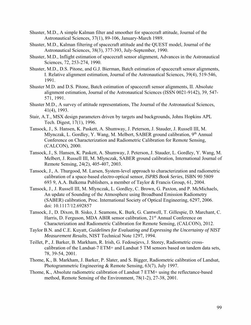
99

Shuster, M.D., A simple Kalman filter and smoother for spacecraft attitude, Journal of the Astronautical Sciences, 37(1), 89-106, January-March 1989.

Shuster, M.D., Kalman filtering of spacecraft attitude and the QUEST model, Journal of the Astronautical Sciences, 38(3), 377-393, July-September, 1990.

Shuster, M.D., Inflight estimation of spacecraft sensor alignment, Advances in the Astronautical Sciences, 72, 253-274, 1990.

Shuster, M.D., D.S. Pitone, and G.J. Bierman, Batch estimation of spacecraft sensor alignments, I. Relative alignment estimation, Journal of the Astronautical Sciences, 39(4), 519-546, 1991.

Shuster M.D. and D.S. Pitone, Batch estimation of spacecraft sensor alignments, II. Absolute alignment estimation, Journal of the Astronautical Sciences (ISSN 0021-9142), 39, 547-571, 1991.

Shuster M.D., A survey of attitude representations, The Journal of the Astronautical Sciences, 41(4), 1993.

Stair, A.T., MSX design parameters driven by targets and backgrounds, Johns Hopkins APL Tech. Digest, 17(1), 1996.

Tansock, J., S. Hansen, K. Paskett, A. Shumway, J. Peterson, J. Stauder, J. Russell III, M. Mlynczak, L. Gordley, Y. Wang, M. Melbert, SABER ground calibration, 9th Annual Conference on Characterization and Radiometric Calibration for Remote Sensing, (CALCON), 2000.

Tansock, J., S. Hansen, K. Paskett, A. Shumway, J. Peterson, J. Stauder, L. Gordley, Y. Wang, M. Melbert, J. Russell III, M. Mlynczak, SABER ground calibration, International Journal of Remote Sensing, 24(2), 405-407, 2003.

Tansock, J., A. Thurgood, M. Larsen, System-level approach to characterization and radiometric calibration of a space-based electro-optical sensor, ISPRS Book Series, ISBN 90 5809 693 9, A.A. Balkema Publishers, a member of Taylor & Francis Group, 61, 2004.

Tansock, J., J. Russell III, M. Mlynczak, L. Gordley, C. Brown, G. Paxton, and P. McMichaels, An update of Sounding of the Atmosphere using Broadband Emission Radiometry (SABER) calibration, Proc. International Society of Optical Engineering, 6297, 2006. doi: 10.1117/12.692857

Tansock, J., D. Dixon, B. Sisko, J. Seamons, K. Burk, G. Cantwell, T. Gillespie, D. Marchant, C. Harris, D. Ferguson, MDA ABIR sensor calibration, 21st Annual Conference on Characterization and Radiometric Calibration for Remote Sensing, (CALCON), 2012.

Taylor B.N. and C.E. Kuyatt, Guidelines for Evaluating and Expressing the Uncertainty of NIST Measurement Results, NIST Technical Note 1297, 1994.

Teillet, P., J. Barker, B. Markham, R. Irish, G. Fedosejevs, J. Storey, Radiometric cross-calibration of the Landsat-7 ETM+ and Landsat 5 TM sensors based on tandem data sets, 78, 39-54, 2001.

Thome, K., B. Markham, J. Barker, P. Slater, and S. Bigger, Radiometric calibration of Landsat, Photogrammetric Engineering & Remote Sensing, 63(7), July 1997.

Thome, K., Absolute radiometric calibration of Landsat 7 ETM+ using the reflectance-based method, Remote Sensing of the Environment, 78(1-2), 27-38, 2001.

100

Thome, K., D. Helder, D. Aaron, J. Dewald, Landsat-5 TM and Landsat-7 ETM+ absolute radiometric calibration using the reflectance-based method. IEEE Transactions on Geoscience and Remote Sensing, 42(12), 2777-2785, 2004.

K. Thome and N. Fox, 2010 CEOS Field Reflectance Intercomparisons Lessons Learned, IGARSS, Vancouver, BC, 2011.

Tobin, D.C., H.E. Revercomb, R.O. Knuteson, F.A. Best, W.L. Smith, N.N. Ciganovich, R.G. Dedecker, S. Dutcher, S.D. Ellington, R.K. Garcia, H.B. Howell, D.D. LaPorte, S.A. Mango, T.S. Pagano, J.K. Taylor, P. van Delst, K.H. Vinson, and M.W Werner, Radiometric and spectral validation of Atmospheric Infrared Sounder observations with the aircraft based Scanning High-Resolution Interferometer Sounder, J. Geophys. Res., 111, D9, 2006.

Tobin, D.C., H.E. Revercomb, R.O. Knuteson, J.K. Taylor, F.A. Best, L. Borg, D. DeSlover, G. Martin, H. Buijs, M. Esplin, R. Glumb, Y. Han, D. Mooney, J. Predina, L. Strow, L. Suwinski, L. Wang, Suomi-NPP CrIS radiometric calibration uncertainty, J. Geophys. Res.:Atmospheres, 118, 10589 - 10600, 2013. doi: 10.1002/jgrd.50809

Topham, T.S., H. Latvakoski, M. Watson, Phase change references for in-flight recalibration of orbital thermometry, ITS 9 AIP Conference Proceedings, Temperature: Its Measurement and Control in Science and Industry, 8, 1552, 993-997, 2013.

Topham, T.S. and F. Best, Microgravity testing of phase change references on the International Space Station, in Earth Science Technology Forum, 2011.

Uprety, S., C. Cao, S. Blonski, and X. Shao, Inter-comparison between Suomi NPP VIIRS, AQUA MODIS and NOAA-19 AVHRR using extended simultaneous nadir overpass in the low latitudes for consistent radiometric calibration, submitted to Journal of Atmospheric and Oceanic Technology, 2013.

Vallado D.A. and W.D. McClain, Fundamentals of Astrodynamics and Applications, 3rd ed. Microcosm Press, 153–162, 2007.

Wang, D., D. Morton, J. Masek, A. Wu, J. Nagol, X. Xiong, R. Levy, E. Vermote, R. Wolfe, Impact of sensor degradation on the MODIS NDVI time series, Remote Sensing of Environment, 119, 55-61, 2012. ISSN 0034-4257, 10.1016/j.rse.2011.12.001. http://dx.doi.org/10.1016/j.rse.2011.12.001

Wang, L., C. Cao, and P. Ciren, Assessing NOAA-16 HIRS radiance accuracy using simultaneous nadir overpass observations from AIRS, Journal of Atmospheric and Oceanic Technology, 24(9) 1546-1561, 2007. doi: 10.1175/jtech2073.1

Wang, L., C. Cao, On-orbit calibration assessment of AVHRR longwave channels on MetOp-A using IASI, IEEE Transactions on Geoscience and Remote Sensing, 46(12) 4005-4013, 2008. doi: 10.1109/tgrs.2008.2001062

Wang, L., C. Cao, M. Goldberg, Intercalibration of GOES-11 and GOES-12 water vapor channels with MetOp IASI hyperspectral measurements, Journal of Atmospheric and Oceanic Technology, 26(9) 1843-1855, 2009. doi: 10.1175/2009, JTecha1233.1

Wang, L.K., X. Wu, Y. Li, et al., Comparison of AIRS and IASI radiances using GOES imagers as transfer radiometers toward climate data records, Journal of Applied Meteorology and Climatology, 49(3) 478-492, 2010, doi: 10.1175/2009, jamc2218.1

101

Wang, L., M. Goldberg, X. Wu, et al., Consistency assessment of Atmospheric Infrared Sounder and Infrared Atmospheric Sounding Interferometer radiances: Double differences versus simultaneous nadir overpasses, Journal of Geophysical Research-Atmospheres, 116, 2011. doi: 10.1029/2010jd014988

White, D.R., M.T. Clarkson, H.W. Yoon, A general technique for calibrating indicating instruments, Metrologia 45, 199-210, 2008. doi:10.1088/0026-1394/45/2/009

Wielicki, B.A., B.R. Barkstrom, E.F. Harrison, R.B. Lee III, G.L. Smith, J.E. Cooper, Clouds and the Earth's radiant energy system (CERES): an Earth observing system experiment, Bulletin of the American Meteorological Society, 77(5), 1996.

Wielicki, B.A., and Coauthors, Achieving climate change absolute accuracy in orbit, Bull. Amer. Meteor. Soc. (BAMS), 94, 1519–1539, 2013. doi: http://dx.doi.org/10.1175/BAMS-D-12-00149.1

Wilthan, B and L.M. Hanssen, Results of an extensive intercomparison of infrared spectral reflectance capabilities, presented at the 19th European Conference on Thermophysical Properties, Thessaloniki, Greece, 2011.

Wolfe, W.L., Introduction to Radiometry, The Society of Photo-Optical Instrumentation Engineers, 1998.

Wright, E.L., Recalibration of the far-infrared brightness temperatures of the planets, Astrophysical Journal, 210, 250-253, 1976.

Wright, E.L. and S. Odenwald, Brightness temperature of Mars: 1979 – 1983, Bulletin of the American Astronomical Society, 12, 456, 1980.

Wright, E.L., Infrared brightness temperature of Mars, 1983-2103, arXiv:astro-ph/0703640v1, 2007.

Wyatt, C.L., Radiometric Calibration: Theory and Methods, New York: Academic Press, Inc., 1978.

Wyatt, C.L., Radiometric System Design, Macmillan Publishing Company, 1987. ISBN 0-02-948800-1

Wyatt, C., V. Privalsky, and R. Datla, Recommended Practice: Symbols, Terms, Units and Uncertainty Analysis for Radiometric Sensor Calibration. NIST Handbook 152, 1998.

Wyatt. C.L., Electro-Optical System Design for Information Processing, McGraw-Hill, Inc., 1991.

Xiong X, K. Chiang, J. Esposito, B. Guenther, and W.L. Barnes, MODIS on-orbit calibration and characterization, Metrologia 40, 89-92, 2003. doi:10.1088/0026-1394/40/1/320

Xiong X., W.L. Barnes, X. Xie, and V.V. Salomonson, On-orbit performance of the Aqua MODIS onboard calibrators, Proceedings of SPIE – Sensors, Systems, and Next Generation of Satellites IX, 5978, 59780U, 2005. doi:10.1117/12.627619

Xiong, X., N. Che, and W.L. Barnes, Terra MODIS on-orbit spectral characterization and performance, IEEE Trans. Geosci and Remote Sens., 44(8), 2196-2206, 2006.

Xiong, X., B. Wenny, N Chen, and J. Dodd, MODIS on-board blackbody performance, 17th Annual Conference on Characterization and Radiometric Calibration for Remote Sensing, (CALCON), Logan UT, 2008.

Xiong X., B.N. Wenny, A. Wu, W. Barnes, and V. Salomonson, Aqua MODIS thermal emissive bands on-orbit calibration, characterization, and performance, IEEE Trans. Geosci. And Remote Sens., 47(3), 803-814, 2009. doi: 10.1109/TGRS.2008.2005109

102

Xiong, X., MODIS on-orbit calibration and lessons learned, 21st Annual Conference on Characterization and Radiometric Calibration for Remote Sensing, (CALCON), Logan, UT, 2012.

Yoon, H.W., Basics and applications of spectroradiometry, Tutorial Session, 19th Conference on Characterization and Radiometric Calibration for Remote Sensing (CALCON), Logan, UT, 2010.

Zhao, T., I. Laszlo, W. Guo, et al., Study of long-term trend in aerosol optical thickness observed from operational AVHRR satellite instrument, Journal of Geophysical Research-Atmospheres, 113(D7), 2008. doi: D07201 10.1029/2007jd009061

Zissis G.J. and W.L. Wolfe, The Infrared Handbook, Office of Naval Research, Department of the Navy, 1978.

Zou, C., M. Goldberg, Z. Cheng, et al., Recalibration of microwave sounding unit for climate studies using simultaneous nadir overpasses, Journal of Geophysical Research-Atmospheres, 111(D19), 2006. doi: D19114 10.1029/2005jd006798

103

COMMON EO SENSOR CALIBRATION REFERENCES

Achieving Satellite Instrument Calibration for Climate Change (ASIC3), Report of Workshop at the National Conference Center, Lansdowne, VA, George Ohring (ed.), May 16-18, 2006.

Art of Radiometry, J.M. Palmer and B.G. Grant, SPIE Press Monograph Vol. PM184, 2009. Data Reduction and Error Analysis for the Physical Sciences, Bevington, P.R and D. K.

Robinson, McGraw-Hill, 1992. Electro-Optical Imaging System Performance and Modeling, Lucien M. Biberman (ed.), SPIE

Press Monograph, Vol. PM96, 2001. Electro-Optical System Design for Information Processing, Clair Wyatt, McGraw-Hill; 2nd

edition, April 1991. Guidelines for Evaluating and Expressing the Uncertainty of NIST Measurement Results, Barry

N. Taylor and Chris E. Kuyatt, NIST Technical Note 1297, 1994. Handbook of Optics, Vol. I, Fundamentals, Techniques, & Design, and Vol. 2, Devices,

Measurements, & Properties, Second edition, McGraw-Hill Professional, 1994. JCGM 100:2008 Evaluation of measurement data - Guide to the expression of uncertainty in

measurement (GUM), BIPM, IEC, IFCC, ISO, IUPAC, IUPAP, OIML, 2008. MSX Bibliography, Version 3.3.2, Cleared for Public Release, SRE Log #0006-2601

https://dcp.mda.mil/. Optical Radiometry, Edited by A. C. Parr, R.U. Datla, and J. L. Gardner, Elsevier Academic

Press, 2005. Radiometric Calibration: Theory and Methods, Clair L. Wyatt, New York: Academic Press,

1978. Recommended Practice; Symbols, Terms, Units and Uncertainty Analysis for Radiometric

Sensor Calibration (NIST Handbook152) Clair L. Wyatt, Victor Privalsky, and Raju Datla, Washington, DC: US Government Printing Office, 1998

Reliable Spectroradiometry, Henry J. Kostkowski, Spectroradiometry Consulting, 1997. SDL/09-576B, MSX data application for future MDA Overhead Persistent Infrared (OPIR)

efforts, Final Report, Space Dynamics Laboratory, Logan, UT, April. 2010 Self-study manual on optical radiation measurements: NBS 910-1 through 910-8, NIST, series of

8 documents from 1977 to 1985, http://www.nist.gov/pml/div685/pub/studymanual.cfm Satellite Meteorology: An Introduction (International Geophysics), Stanley Q. Kidder, Academic

Press, 1995. The Infrared Handbook, William L. Wolfe and George J. Zissis, General Dynamics, Revised

Edition, 1985. The Infrared and Electro-Optical Systems Handbook [8 volume set], Joseph S. Accetta and

David L Shumaker, ERIM, SPIE Press, 1993. Traceable Temperatures, An Introduction to Temperature Measurement and Calibration, J.V.

Nicholas and D.R. White, Wiley, 2001.

104

ACRONYM LIST

ABIR Airborne Infrared Sensor ACRIM Active Cavity Radiometer Irradiance Monitor AERI Atmospheric Emitted Radiance Interferometer AI&T Assembly, Integration, and Test ASIC3 Achieving Satellite Instrument Calibration for Climate Change BASS Broadband Array Spectrograph System (Aerospace) BIPM International Bureau of Weights and Measures (French: Bureau International

des Poids et Measures) BRDF Bi-Directional Reflectance Distribution Function Cal/Val Calibration and Validation CCS Calibration Control System CEOS Committee on Earth Observing Satellites CERES Clouds and the Earth’s Radiant Energy System CIPM International Committee for Weights and Measures CLARREO Climate Absolute Radiance and Refractivity Observatory CMS Control and Monitor System COBE Cosmic Background Explorer COTS Commercial Off The Shelf CrIS Cross-Track Infrared Sounder CSO Closely Spaced Objects DITL Day In The Life DN Digital Number DO Dark Offset DoD Department of Defense DS Deep Space ECI Earth Centered Inertial EFOV Effective Field if View (Solid Angle) EMI Electromagnetic Interference EMC Electromagnetic Compatibility EO Electro-Optical EOD Energy On Detector ERF Edge Response Function ERB Earth Radiation Budget ESE Electronic Support Equipment ESR Electrical Substitution-Type Radiometers FIRST Far-Infrared Spectroscopy of the Troposphere FPA Focal Plane Array FOR Field Of Regard FOV Field Of View FTI Frontier Technology, Inc. FTS Fourier Transform Spectrometer GEO Group on Earth Observations GIFTS Geosynchronous Imaging Fourier Transform Spectrometer GOES Geostationary Operational Environmental Satellites GSE Ground Support Equipment GSICS Global Space-based Inter-Calibration System

105

GUM Guide to the Expression of Uncertainty in Measurement HIRS High Resolution Infrared Radiation Sounder IASI Infrared Atmospheric Sounding Interferometer ICT Internal Calibration Target ICU Internal Calibration Unit IEC International Electrotechnical Commission IFC In-Flight Calibration Source IFOV Instantaneous Field of View IR Infrared ISO International Organization for Standardization JCGM Joint Committee for Guides in Metrology JPL Jet Propulsion Laboratory JPSS Joint Polar Satellite System K Kelvin LASP Laboratory of Atmospheric and Space Physics, Univ. of Colorado, Boulder LBIR Low-Background Infrared Facility, NIST LEO Low Earth Orbit LOS Line of Sight LSF Line Spread Function LTT Long-Term Trending LWIR Long-Wave Infrared MKS Meter-Kilogram-Second MODIS Moderate Resolution Imaging Spectroradiometer MSX Midcourse Space Experiment MTF Modulation Transfer Function MTSAT Multifunctional Transport Satellite MWIR Mid-Wave Infrared NAS Near Angle Scatter NASA National Aeronautics and Space Administration NCC National Calibration Center at NOAA NDVI Normalized Difference Vegetation Index NEdN Noise Equivalent Radiance Difference NEdT Noise Equivalent Delta Temperature NEI Noise Equivalent Irradiance NEP Noise Equivalent Power NER Noise Equivalent Radiance NGC Northrop Grumman Corporation NIR Near Infrared NIST National Institute of Standards and Technology NMI National Metrology Institutes NOAA National Oceanic and Atmospheric Administration NUC Non-Uniformity Correction NVLAP National Voluntary Laboratory Accreditation Program OAR Off-Axis Response OBC On-Board Calibrator OIML International Organization of Legal Metrology OMI Ozone Monitoring Instrument OOB Out of Band

106

PICS Pseudo-Invariant Calibration Sites PIRR Peak Irradiance Responsivity PRF Point response function PRR Peak Radiance Responsivity PRT Platinum Resistance Thermometer PSF Point Spread Function QCL Quantum Cascade Laser RDR Raw Data Record RSR Relative Spectral Response ROLO Robotic Lunar Observatory RTC Radiative Transfer Code SABER Sounding of the Atmosphere using Broadband Emission Radiometry SDL Space Dynamics Laboratory SDR Sensor Data Records SDSM Solar Diffuser Stability Monitor SeaWiFS Sea-Viewing Wide Field-of-View Sensor SED Spectral Energy Distributions SI International System of Units (French - Système International)

SIRCUS NIST Spectral Irradiance and Radiance Responsivity Calibrations Using Uniform Sources

SNO Simultaneous Nadir Overpass S-NPP Suomi-National Polar-orbiting Partnership SNR Signal-to-Noise Ratio SPIRIT (III) Spatial Infrared Imaging Telescope SSA Space Situational Awareness SUT Sensor Under Test SWIR Short-Wave Infrared TDI Time Delay and Integration THOR Thermal and Optical Research Chamber TI Technical Intelligence TIMED Thermosphere-Ionosphere-Mesosphere Energetics and Dynamics TLYF Test Like You Fly TOA Top of Atmosphere TRR Test Readiness Review TSI Total Solar Irradiance TVAC Thermal Vacuum UAH University of Alabama in Huntsville USGS U.S. Geological Survey V&V Verification and Validation VIIRS Visible Infrared Imager Radiometer Suite VIM International Vocabulary of Metrology – Basic and General Concepts and

Associated Terms WMO World Meteorological Organization WORM Write Only Read Many

107

GLOSSARY OF TERMS

The terms included in this glossary are defined as they apply to EO sensors, radiometric calibration, and remote sensing.

Absolute Calibration Absolute calibration is defined in terms of a sensor's response on a physical, real-world scale, measured in internationally defined and accepted units (SI units, for example).

Alignment/Co-Alignment Alignment and co-alignment refer to the degree of co-location of one sensor or array FOV with another, or with any defined baseline angle. Misalignments can include both rotation and offset components relative to the baseline optical axis.

Sensor Alignment Matrix The sensor alignment matrix is a unitary rotation matrix relating sensor coordinates to spacecraft coordinates. The sensor alignment matrix is unique for each sensor.

Atmospheric Transmission Atmospheric transmission typically refers to the transmission of light as a function of wavelength along the line of sight. As light (photons) passes through the atmosphere, it interacts with the molecular species that make up the atmosphere (H20, CO2, O3, CO, CH4, N2O, etc.), with difference molecular species absorbing, scatterings and re-emitting different wavelengths of light. At some wavelengths, the atmosphere is very transmissive, while at other wavelengths it is very opaque. Atmospheric transmission is highly dependent on atmospheric concentrations, temperature, and pressure (all of which vary with altitude) along the LOS. Computer codes such as MODTRAN and HITRAN are very good at accurately deriving atmospheric transmission based on user input information.

Background Background is a term that is used loosely in EO sensor terminology and can have any the following meanings:

Sensor Background/Sensor Dark Offset (DO): A sensor’s DO is its response with zero input radiance. If an IR sensor has a warm optical system (or warm optical components), the sensor’s DO will contain self-emission from the optical system.

Background Source/Dark Background: An ideal background source/dark background is a target or scene that reflects and emits zero radiance. In practice, a background source reflects and emits radiance that is below the sensor’s NER/NESR. For most IR sensors the background source must be both light tight and cold enough such that the total reflected and emitted radiance is below the NER/NESR or self-emission from the sensor’s optical system.

Background Clutter: Unwanted radiometric intensity and/or spatial structure in a target scene.

Bakeout Hardware bakeout is part of the contamination control process. All flight and test hardware must meet cleanliness and material outgassing requirements prior to TVAC testing and flight. For hardware bakeout, components are placed into a TVAC chamber at specific temperature and pressure levels for a specified period of time to insure cleanliness prior to TVAC testing.

108

Blackbody Blackbody sources are used as radiometric standards in IR sensor calibration. An ideal blackbody source perfectly matches Planck’s emissivity law and has zero reflectance. In practice, a blackbody source approximates Planck’s emissivity law, has an accurately known surface temperature, is highly uniform spatially and has very low reflectance. All non-ideal performance characteristics must be quantified in the blackbody’s radiometric uncertainty.

Calibration Coefficients See Calibration Equation / Calibration Coefficients

Calibration Data Products Calibration data products are the numeric values that are produced during calibration and quantify an EO sensor’s performance. Calibration data products include calibration coefficients and other quantifiable calibration parameters such as IFOV, RSR, NER, etc. Calibration data products are typically delivered as computer data files and are documented in the calibration report.

Calibration Equation / Calibration Coefficients A calibration equation is a mathematic model of a sensor response, converting the sensor output response to SI radiance units. The calibration coefficients are the calibration equation parameter values that are quantified during calibration.

Calibration Parameters Calibration parameters refer to information generated (or that will be generated) during the course of a calibration that quantifies and/or describes the EO sensor performance.

Calibration Plan The calibration plan is a written document that lists top-level assumptions, parameters, measurement equipment and methods, and data collection and analysis methods that will be implemented to achieve calibration of a specific sensor. The data collection plan typically identifies a list of data collection procedures and refers to them for specific details for a given calibration measurement.

Calibration Procedures A calibration procedure is a written document that lists a specific sequence of events that implement a given calibration measurement. The procedure includes logsheets and/or checklists for recording and documenting the measurement for reference during data analysis. See Data Collection Procedure

Co-Alignment See Alignment/Co-Alignment

Collimator A collimator is piece of optical test hardware that creates a simulated point source.

Component-Level Testing Component-level testing refers to tests performed on the components or subassemblies of an EO sensor prior to being integrated into the EO sensor assembly.

Contamination Control Contamination control is the process of keeping an EO sensor payload clean enough to accomplish its mission. Contamination control is addressed at the spacecraft and payload level,

109

with requirements flowing down to the EO sensor handling and environmental exposure during calibration testing. Contamination control must be included in the calibration plan or addressed in a separate contamination control plan.

Counts See Data Number / Digital Number

Coverage Factor (k) Coverage factor is the number of standard deviations included in the reported uncertainty. For a normal distribution, k = 1, k = 2, and k = 3 provide confidence levels of approximately 68 %, 95 %, and 99.7 %.

Cross-Calibration The process of deriving or updating the calibration parameters (typically radiometric responsivity) of the sensor being calibrated, by comparing the response of the sensor being calibrated to the known and trusted response of a calibrated sensor viewing the same earth scene at the same time.

Cryogenic Cryogenic refers to the very low temperatures required to test some EO sensors, especially focal plane arrays in the LWIR wavelengths. Cryogenic systems require high-vacuum thermal control equipment, and typically reach extremely low temperatures through cooling provided by liquefied noble gasses (helium, neon, argon, or xenon), liquefied or frozen nitrogen, and/or frozen hydrogen. Cryogenic temperatures can also be achieved with specialized mechanical cryocoolers.

Dark Noise See Noise - Dark Noise

Data Collection Procedure The data collection procedure, a subset of the overall test procedure, contains test objectives, configuration requirements, test entry criteria, configuration steps, data collection steps and other pertinent information specific to a given calibration test. The test conductor should be familiar with the test objectives, hardware and data collection procedure prior to starting the test. During testing, initials and signature blocks should be completed, and any exceptions, deviations and anomalies should be recorded in the data collection procedure, creating an as-run data collection procedure for archival.

Data Management Data management refers to the task of collecting, quality checking, organizing, cataloging, archiving, processing and distributing all test data, including: sensor response and metadata, environmental data, source configuration information and reading values, and any other ancillary data.

Data Numbers / Digital Numbers (DN) The response of most modern EO sensors is captured and stored in computer data formats that are generically referred to as Data Numbers (DN) or Digital Numbers (DN). EO sensor output is often referred to as ‘response counts’ or simply ‘counts'.

Data Products See Calibration Data Products

110

Distortion / Optical Distortion Distortion occurs when image magnification in an EO sensor optical systems varies with position within the image, causing straight lines (generally conceptual rather than literal) in the object to be mapped into curved lines in the image.

Distortion Map / Distortion Correction The distortion map provides the equations needed to manipulate digitized EO sensor images to correct for the optical distortion introduced in the sensor. The distortion map is unique to each EO sensor. Based on the sensor design, the distortion correction equation may take the form of Zernike polynomials, or it could also be a high order (typically 3rd or 5th order) polynomial. Some sensor configurations may require a more complex equation.

Dynamic Range The dynamic range is the response range over which sensor values are valid. It is typically defined as the response range between dark noise and hard saturation.

Earth's Limb Limb is defined as the outer edge of the apparent disk of a celestial body (Merriam-Webster). EO sensors can view the Earth limb from Earth orbit. It is typical when making Earth limb measurements to specify a ‘tangent height’ within Earth limb - defined as minimum distance between the sensor LOS and the hard Earth, which occurs at the tangent point.

Earth’s Energy Balance / Earth’s Energy Budget Earth's energy balance/budget is the net difference between the total energy received by the Earth vs. the total lost, resulting in net global temperature change. This process is driven by radiative heat transfer, creating a quantitative measurement role for EO sensor technology.

Earth-Observing Sensor (EOS) An EOS is sensor making quantitative measurements of the Earth or Earth's limb from Earth orbit. In the more restrictive sense, EOS may apply only to sensors involved in missions related to global climate change.

Effective Bandpass Effective bandpass is a figure of merit, representing an EO sensor’s spectral bandwidth in units of wavelength, frequency or wavenumber. Effective bandpass is the bandwidth an ideal EO sensor would have given a spectral responsivity of 1 within the spectral bandpass and 0 outside.

Effective Field of View (EFOV) EFOV solid angle is an optical sensor spatial figure of merit that represents the field-of-view solid angle in units of steradians. Given an EFOV, an ideal sensor would have a spatial responsivity of 1 within the solid angle and 0 outside.

Emissivity Emissivity is the ratio of the energy radiated by an emissive surface relative to that of an ideal blackbody source at the same temperature. It is generally related as a function of wavelength or frequency, emissivity values range from 0 to 1.

End-to-End Calibration End-to-end calibration refers to the calibration of a complete system, from input aperture to data products, to capture all possible effects that may be features of a sensor and data system.

111

Ensquared Energy / Energy on Detector (EOD) EOD is the fraction of the total energy in a point source that falls on a single pixel when centered on said pixel.

Electro-Optical (EO) Sensor An EO sensor is a system designed to use optical and electronic phenomena to characterize a remote scene or source for information extraction purposes.

Extended Source An extended source is a source of electromagnetic radiation that is not resolved to a single point or direction in space, and has a greater extent than the IFOV of the sensor involved. In the laboratory, an extended source is often implemented by a flat plate with a surface treatment to maximize emissivity and uniformity.

Field of Regard (FOR) See Field of View

Field of View (FOV) The FOV of a sensor is a numeric value representing the angular extent of an EO sensor’s response, generally expressed in radians, arc-degrees, or arc-minutes.

IFOV: Individual FOV or instantaneous FOV; FOV of a single pixel in an EO sensor containing an imaging FPA.

FOR: Field-of-regard; The full range of FOV that may be seen by an instrument including the range of all arrays, zoom modes, and pointing mirrors in the instrument; also includes EO sensor pointing mechanisms such as gimbals and turrets.

Filter In EO sensor parlance, filter refers to an optical filter(s) that is placed in the optical path of an EO sensor to select, restrict, reject, limit, or adjust an EO sensor response to specific wavelengths/frequencies of light.

Bandpass: The range of desired wavelengths/frequencies to be passed by an optical filter. Generally defined by the cut-on and cut-off wavelengths/frequencies of the optical filter.

In-Band Response: EO sensor response to the optical wavelengths/frequencies within the desired optical filter bandpass.

OOB Blocking: The ability of an optical filter (or optical system) to reject optical energy outside the desired bandpass. May also refer to filter design specifications regarding the ability to reject optical energy outside the desired filter bandpass.

OOB Leakage: Undesired optical energy that passes through an optical filter (or optical system) that has a spectral location outside the desired spectral bandpass.

OOB Response: An EO sensor’s response to OOB leakage.

Transmittance: Ratio of the open-path throughput of an optical path with and without the filter. Generally expressed as a function of wavelength or optical frequency, transmittance values range from 0 to 1, or 0 to 100 % if expressed in percent transmittance.

112

Focus The focus, also called an image point, is the point where light rays originating from a point on an object converge to a minimum. Although the focus is conceptually a point, physically the focus has a spatial extent, called the blur circle, which is caused by optical aberrations. In the absence of significant aberrations, the smallest possible blur circle is the Airy disc, which is caused by diffraction from the optical system's aperture. Aberrations tend to get worse as the aperture diameter increases, while the Airy circle is smallest for large apertures.

Best Focus / Optimum Focus Verifying sensor focus is part of sensor calibration. Some sensors are equipped with mechanisms to adjust the focus while the instrument is in operation. For these sensor the optimum focus is found by adjusting the focus when the sensor is viewing a point source. For sensors not equipped with a focus adjustment, the calibration hardware presents a point source to the sensor and then changes the focus of the source with the calibration hardware allowing the optimum focus to be found.

Focus Requirements

For imaging sensor systems, a focus requirement is generally included in the sensor performance specifications, which can be specified in terms such as ensquared energy. The sensor is generally considered to be within focus when the ensquared energy is maximized and/or greater than a specified threshold requirement.

Goniometric Goniometric measurements are those that involve angular positions or angular distances. In EO sensor calibration, goniometric parameters include: alignment, PRF, distortion, pointing accuracy, near angle scatter (NAS), and large angle scatter.

Ground Calibration See Pre-Launch Calibration

Ground Support Equipment (GSE) GSE is the collection of equipment used to operate a remote sensing instrument during ground testing, operations, and calibration. GSE is typically very sensor specific/custom, and includes: monitoring equipment/software, mechanical support hardware, electrical power, thermal control hardware/software, communications hardware/software, data management hardware/software, and so forth.

Sensor GSE: Hardware and software that directly supports sensor operation either independently or as part of a larger ground calibration test campaign.

Electrical GSE (ESE): Hardware and software that extends capabilities to support extensive pre-launch ground calibration and testing. ESE generally includes a robust data management system to accommodate large data volumes generated during ground testing.

Internal Calibration Unit (ICU) ICU is a generic term for a radiance and/or spectral reference source that is contained within the EO sensor’s optical path. In some cases the ICU may not qualify as a true calibration source in that it does not have inherently known calibration properties. Rather, the ICU is highly repeatable and can be a link to a true calibration source during pre-launch calibration by

113

sequentially viewing the ICU and ground calibration source. ICUs may also be known by the synonyms internal stimulator (stim) sources or internal reference sources.

IFOV See Field of View → IFOV

In-Band Response See Filter → In-Band Response

Integration Time / Integration Modes Integration time / integration modes refers to the length of time a detector signal is accumulated/integrated between resets. Multiple integration times are implemented in detectors to extend the response dynamic range. In snapshot read/charge transfer detectors, integration time is reset when the detectors are read. In up-the-ramp sampling, detectors are sampled multiple times between resets. A set of discrete integration times can also be known as integration modes.

Integration Time Normalization / Integration Mode Normalization Integration time (mode) normalization is a calibration data product that is applied as part of the calibration equation (after EO sensor measurements are performed) to rescale data collected at multiple integration times to a common reference (generally relative to the responsivity of the shortest integration time).

Inter-Satellite Calibration See Cross-calibration

Irradiance / Spectral Irradiance Irradiance is an entity of flux that describes a point source or a source of a fixed size and distance such as the Sun when viewed from Earth. When irradiance includes wavelength dependence it is called spectral irradiance. Generalized units of spectral radiance are Watts/(cm2 µm) or Photons/sec/(cm2 µm).

Jitter Jitter is unwanted mechanical vibrations in an EO sensor’s internal optical path or between the EO sensor and the calibration source/measurement target, or within the optical path of the calibration source (e.g., collimator), resulting in blurring of the energy at the EO sensor’s focal plane. Jitter can be especially problematic when performing point source measurements during pre-launch calibration.

Jones’ Source Jones’ source refers to a near field small area source, sometimes referred to as a Jones’ method source (Wyatt 1978). It is a small area source that underfills the sensor entrance aperture, while filling the sensor field stop.

Large-Angle Scatter / Off-Axis Scatter Large-angle or off-axis scatter is unwanted signal that originates from sources that are outside of a sensor’s direct FOV. See Off-Axis Rejection

Linearity / Non-Linearity Linearity and non-linearity are terms used to describe the proportional relationship between an incremental change in target radiance and the incremental change in an EO sensor’s output

114

response, over the EO sensor’s dynamic range. In a perfect EO sensor system, an incremental percent change in the input radiance of a source should produce the same incremental percent change in the EO sensor output response, regardless of where in the sensor dynamic range the measurement occurs. Measuring an EO sensor’s linearity, creating a linearity correction function, and creating a linearity correction uncertainty estimate are key components of most EO sensor calibrations.

Line-of-Sight (LOS) LOS is the direct optical path between an EO sensor and a measurement target. LOS may include atmospheric species and/or obscurations along the path.

Long Term Repeatability See Repeatability – Long-Term

Measurement Accuracy (See JCGM 200:2012, 2.13) Measurement accuracy is the closeness of agreement between a measured quantity value and a true quantity value of a measurand. The concept ‘measurement accuracy’ is not a quantity and is not given a numerical quantity value. A measurement is said to be more accurate when it offers a smaller measurement error. Measurement accuracy is also referred as ‘accuracy of measurement’ or ‘accuracy’. However in remote sensing literature ‘accuracy’ is often used to represent ‘bias’. Bias is an estimate of a systematic measurement error that is the component of measurement error in replicate measurements that remains constant or varies in a predictable manner.

Measurement Requirements Measurement requirements are the set of specifications that define the performance to be achieved by a remote sensing instrument. Measurement requirements must be defined in consultation and collaboration with program management, mission scientists, and instrument engineers to reconcile program and science needs and desires with technological realities, and to ensure that all parties understand the resulting measurement requirements in the same way.

Measurement Uncertainty (See JCGM 200:2012, 2.26) Measurement uncertainty is the dispersion of the values being attributed to a quantifiable physical property; measurement uncertainty defines an interval that is likely to enclose the true value of that quantity. Measurement uncertainty contains components arising from both the systematic and the random effects. The more limited the accuracy and precision of a measurement instrument, the larger the measurement uncertainty. Measurement uncertainty is also referred to as uncertainty of measurement or, in short, uncertainty.

Modulation Transfer Function (MTF) MTF is a measure of an EO sensor’s spatial resolving capability, which is represented by the normalized Fourier transform of the PSF. MTF is a combined representation of the spatial resolution and image quality of an imaging system, represented in terms of the normalized spatial frequency response.

Near Angle Scatter (NAS) NAS (or small-angle scatter) is unwanted signal that originates from sources that are inside the FOR and more generally in the local neighborhood. NAS typically originates from filters, beamsplitters, and baffle edges located near or within the optical path of the sensor.

115

Noise Noise is unwanted variability in electronic signals and/or digitally sampled measurement values. In most measurement scenarios, measurement noise limitations challenge measurement objectives and are a major contributor to overall measurement uncertainty.

Noise – Dark Noise Dark noise is the EO sensor noise observed when the sensor has no measureable input radiance. Dark noise can be expressed in counts or in terms of either noise equivalent radiance or irradiance. Noise equivalent radiance (NER) of a sensor is its dark noise expressed in units of radiance. Noise equivalent irradiance (NEI) of a sensor is its dark noise expressed in units of irradiance. Noise equivalent spectral radiance and noise equivalent spectral irradiance are referred to as NESR and NESI, respectively.

Noise – Photon Noise Photon noise is caused by the random arrival of photons and signal conversion at the detector. It is generally considered as a Poisson statistical distribution, which means that the signal variance is proportional to the mean value.

Noise – Noise Equivalent Delta Temperature (NEdT) NEdT is the target-to-background temperature difference that produces a signal-to-noise ratio of unity.

Noise – Noise Equivalent Irradiance (NEI) NEI is the flux density at the entrance pupil of the optical system that produces an output signal equal to the system’s noise. It is used to characterize the response of a system to a point source target.

Noise – Noise Equivalent Radiance (NER) NER is the entity of radiance that is most appropriate for the description of radiant flux from an extended area source. The NER is the amount of radiant flux that produces a signal equal to the system’s noise when viewing an extended source.

Non-Linearity See Linearity

Non-Uniformity Correction (NUC) NUC quantifies each pixel’s responsivity relative to the array mean (or median) responsivity when illuminated by a uniform source. NUC is typically computed for each FPA configuration (integration time, bias voltage, gain, etc.) combination.

Off-Axis Rejection Off-axis rejection is the ability of a telescope to reject signal that originates from sources outside of the telescope's direct FOV, such as signal from the surface of the Earth when viewing the Earth's limb.

Operational Envelope The operational envelope is the range of values for operational parameters, such as temperature, solar illumination, or radiation exposure, over which a remote sensing instrument is expected to provide results consistent with the overall calibration uncertainty.

116

Operational Environment The operational environment describes the conditions under which a remote sensing instrument is expected to function. These conditions must be simulated during ground testing and calibration. For example, an instrument to be operated in orbit must be operated in a thermal-vacuum space simulation chamber for ground testing to identify and characterize all behaviors that may be expected to arise during operation.

Out-of-Band (OOB) Blocking See Filter → OOB Blocking

Out-of-Band Leakage See Filter → OOB Leakage

Out-of-Band Response See Filter → OOB Response

Optical Density Optical density is the log (base 10) of the attenuation of a filter, typically used when referring to neutral density or spectrally flat filters used to attenuate a beam. For example, a neutral density filter of 1 % transmission has an optical density of 2.

On-Orbit Calibration See Post-Launch Calibration

Peak Irradiance Responsivity (PIRR) PIRR is a calibration data product that converts corrected EO sensor response values (in corrected response units, such as counts) into irradiance units, such as W/cm2 or Jansky’s. PIR is dependent on sensor response corrections and produces a final result that is accurate for a monochromatic source located at the RSR peak wavelength.

Peak Radiance Responsivity (PRR) PRR is a calibration data product that converts corrected EO sensor response values (in corrected response units, such as counts) into radiance units, such as W/(cm2·sr). PRR is dependent on sensor response corrections and produces a final result that is accurate for a monochromatic source located at the RSR peak wavelength.

Photon Noise See Noise – Photon Noise

Planck’s Equation The equation describing spectral radiance emitted by an ideal blackbody. In fundamental units the equation is:

2

5 2

2 1

1hc kT

hc Watts

e m sr m

where h is Planck's constant, c is the speed of light, k is Boltzmanns constant, T is temperature in kelvin, and is wavelength in meters. The units have been written to emphasize that the result is a flux density (per area and solid angle) per wavelength.

117

Point Response Function (PRF) The PRF describes the sensor’s normalized response to a point source. The shape of the PRF is determined from optical diffraction, geometric image quality, detector spatial response, optical scatter, detector-to-detector electrical crosstalk, and jitter. The PRF is the PSF of the sensor as it is sampled by the FPA.

Point Spread Function (PSF) The PSF is the two dimensional profile of the flux density produced by a point source on the image plane of a remote sensing instrument. The shape of the PSF is determined from optical diffraction, geometric image quality, optical scatter, and jitter. In the case of diffraction-limited performance, the PSF is the cross section of the airy disk or optical blur.

Point Source A point source is a source of electromagnetic radiation that is resolved in the ideal case to a single point or direction in space. For example, a natural star is an ideal point source. In the laboratory on the ground, a point source is simulated using an optical collimator.

Pointing and Goniometric Parameters Pointing and goniometric parameters are coefficients and characterizations that describe the relationship between the position of an object observed by a remote sensing instrument and the true position in object space. They include parameters that describe telescope distortion and distortion correction, conversion of focal-plane position to object-space angle, IFOV, and optical image quality.

Polarimeter A polarimeter is a remote sensing instrument designed to have the capability to measure and characterize polarization.

Polarization Polarization is the degree of alignment of the electric field in a beam of electromagnetic radiation. Polarization is described in terms of two polarization components rotated 90 degrees from each other (horizontal and vertical polarization components). In general, an electromagnetic beam is a combination of the following three possibilities:

Unpolarized: A beam of electromagnetic radiation in which the electric field vector changes constantly and randomly.

Linear Polarization: A beam of electromagnetic radiation in which the horizontal and vertical polarization components are fixed and in phase, resulting in an electric field that oscillates in one angle.

Circular Polarization: A beam of electromagnetic radiation in which the horizontal and vertical polarization components are fixed but shifted in phase, resulting in a rotating electric field angle.

See Responsivity Domains

Polarization Sensitivity Polarization sensitivity is the degree to which a remote sensing instrument is sensitive to radiation of one polarization state over another.

118

Post-Launch Calibration A general term that encapsulates any and all calibration activities that occur after a satellite-based EO sensor is on-orbit (thus post-launch calibration may also be referred to as on-orbit calibration). The scope of the post-launch calibration varies from program-to-program and sensor-to-sensor, and includes considerations such as mission objectives, measurement requirements, mission operations capabilities, sensor data collection capabilities, and the ability to downlink low-level sensor response data to the ground. Post-launch calibration activities are included in the calibration plan and are executed according to the post-launch calibration procedures.

Pre-Launch Calibration Pre-launch calibration (or ground calibration) is the sequence of measurement and characterization that takes place during and after instrument assembly and integration, prior to launch. Pre-launch calibration provides the best or only chance to measure some parameters such as spectral response, linearity, and polarization sensitivity, and also provides an important quality control and validation function to prevent unpleasant surprises and disappointment after launch.

Quicklook Analysis A quicklook analysis is a preliminary look at the data and is used to verify dataset completeness and integrity before moving on from a data collection task.

Radiance / Spectral Radiance Radiance is an entity of flux that describes an extended source. When radiance includes wavelength dependence it is called spectral radiance. Generalized units of spectral radiance are watts/(cm2sr µm) or photons/(sec cm2sr µm).

Radiometer A radiometer is a remote sensing instrument designed to measure the total quantity of radiation in a limited bandwidth. A radiometer may be more specifically described by the wavelength region in which it operates, such as infrared radiometer or microwave radiometer.

Broadband Radiometer: A radiometer that integrates radiation across a wide wavelength range, as opposed to a spectrometer, which measures radiation at specific wavelengths or within very narrow wavelength bands.

Radiometric Calibration Radiometric calibration is the process of deriving coefficients, identifying and describing behaviors, and characterizing all aspects of a remote sensing instrument to relate the response of the sensor to a known quantity of flux entering the system. A system that has undergone this process can then infer the value of an unknown quantity of flux based on the response of the instrument.

Radiometric Model A radiometric model is a mathematical model of response of a sensor to observed scenes and sources, typically implemented on a computer, to facilitate rapid calculation of multiple parameter cases. A detailed radiometric model is essential to successful calibration planning to validate calibration source configurations and equipment designs. See Sensor Performance Model

119

Real-Time Real-time refers to providing immediate feedback, without delay for observation, processing, or analysis. A monitor of sensor output that shows instantaneous changes in response as sources are adjusted during test setup is often called a real-time display.

Relative Spectral Responsivity (RSR) A radiometer’s RSR is its peak-normalized response to radiation at different wavelengths both within (in-band) and outside (out-of-band) its spectral bandpass. The RSR is used to calculate the effective flux for absolute responsivity calibrations, and to interpret flight data.

Remote Sensing Remote sensing is the technique of measuring the reflected or emitted radiation from an object to infer characteristics of the object that can not be measured directly. Remote sensing measurements are performed passively.

Repeatability Repeatability refers to the stability of the response of a remote sensing instrument over time. Repeatability is defined over short, medium, and long time intervals as follows:

Short-Term: Repeatability or stability of a measurement between adjacent samples or within a single integrated measurement interval. Short-term repeatability is quantified from measurement noise with a timescale of typically seconds to minutes. See Noise

Medium-Term: Repeatability or stability of response from a stable input between consecutive or succeeding integrated measurement intervals. Medium-term repeatability is typically quantified via benchmark tests that are included as part of a measurement sequence. Medium-term repeatability sources may include on-board stimulator sources, vicarious ground sources, and stellar references. The medium-term repeatability timescale is typically minutes to hours.

Long-Term: Repeatability or stability between widely separated measurement intervals. Long-term repeatability is typically quantified via benchmark tests that periodically measure constant radiometric source(s) over the life of the sensor. Long-term repeatability sources may include on-board stimulator sources, vicarious ground sources, and stellar references. The long-term repeatability timescale is typically hours to days, up to the lifetime of the sensor.

Responsivity Domains Remote sensing systems provide information about an object by recording the response to radiation coming from the object in one or more of five responsivity domains:

Radiometric: Response to electro-magnetic radiant energy as a function of quantity (relative and/or absolute)

Spatial: Energy distribution as a function of position

Spectral: Energy distribution as a function of wavelength or frequency

Temporal: Variation of energy distribution as a function of time

Polarization: Orientation of electric field vector

120

Calibration measurements seek to limit interaction between responsivity domains by varying parameters in one domain while holding parameters pertaining to other domains constant.

Saturation Saturation is the state or behavior of a remote sensing instrument when the upper limit of dynamic range is met or exceeded. Typically, the charge storage or transfer capacity of individual pixels is exceeded, leading to anomalous effects in other pixels. Saturation effects begin to appear as the limit is approached and met and become more severe beyond the limit.

Soft Saturation: Saturation effects that begin to appear as the limit of dynamic range is approached and may be amenable to correction, resulting in useful data.

Hard Saturation: Saturation effects that occur when the limit of dynamic range is exceeded and that cannot be corrected to produce useful data.

Scanner / Scanning Sensor A scanner or scanning sensor uses a moving FOV or viewing angle to achieve greater FOR, as opposed to a sensor that maintains a static viewing angle. See Starer/Staring Sensor

Push-Broom: A scanning sensor in which the FOV is moved parallel to the direction of motion of the sensor.

Wisk-Broom: A scanning sensor in which the FOV is moved perpendicular to the direction of motion of the sensor.

Sensor Performance Model The sensor performance model is a mathematical model of a sensor's response, including noise and background sources, that is typically implemented on a computer to facilitate rapid calculation of multiple parameter cases. A detailed sensor performance model is essential to successful calibration planning to validate calibration source configurations and equipment designs. See Radiometric Model

SI (International System of Units) The International System of Units (French - Système International) is the system of scientific units used for scientific, acceptable radiometric calibration.

Spectral Resolution Spectral resolution is a measure of a sensor’s power to resolve features in the electromagnetic spectrum. It is defined by the equation R = λ/Δλ where Δλ is the smallest difference in wavelengths that can be distinguished at a wavelength of λ.

Spectrometer A spectrometer is an instrument that makes measurements in multiple narrow bands or discrete wavelengths (spectral bins) to trace out the shape of an emission or transmission curve.

Multi-Spectral: Measurements containing multiple spectral bins or bandpasses.

Hyper-spectral: Oversampled spectrally or containing many spectral bins.

121

Starer / Staring Sensor A starer or staring sensor is a sensor that maintains a static FOV or viewing angle, as opposed to one that moves the FOV by means of a scan mirror, for example. See Scanner/Scanning Sensor

Steradian A steradian is a unit of solid angle, or an angle in two dimension, that describes the volume enclosed by the angle subtended in each dimension.

Stierwalt Effect The Stierwalt effect refers to out-of-band leakage through a filter of light scattered at high oblique angles by defects in the filter coating layers. When placed immediately in front of a detector, a filter showing the Stierwalt effect will show higher out-of-band transmission than would be expected from standard transmittance measurements where the detector is far from the filter.

Strawman Calibration Planning Strawman calibration planning is an iterative method for obtaining consensus on a calibration approach among project leadership, scientists, and engineers. The goal is to produce an optimum calibration while minimizing cost, schedule, and uncertainty. The strawman plan ideally addresses the entire duration of the sensor lifetime, establishes the initial plan for calibration measurement methods, provides a first draft of measurement combinations, and makes budgeted estimates of uncertainty.

System-Level Calibration See End-to-End Calibration

Technical Intelligence (TI) TI is a broad term for the end product of a remote sensing instrument designed for military use such as surveillance and reconnaissance.

Temporal Frequency Responsivity Temporal frequency responsivity describes a sensor's response change with respect to changes in input signal as a function of time. Through Fourier analysis, temporal frequency responsivity is typically reported in terms of frequency. The temporal frequency responsivity of a sensor characterizes its response to time-varying signals.

Test Conductor The test conductor executes specific calibration test procedures to accomplish specific calibration tests. Test conductor responsibilities may be distributed between more than one test conductor to cover all calibration tests, depending on the scope of the calibration. The test conductor's role is generally filled by a calibration engineer.

Traceability Traceability is the property of a measured value whereby it can be related through an unbroken chain of calibrations, with quantitative and documented uncertainties to an original standard of measurement (such as SI).

Transmittance See Filter → Transmittance

122

TVAC / TVAC Chamber TVAC testing simulates the space environment or other conditions that may be of interest during test and calibration of an electro-optical instrument. This testing is performed in a TVAC chamber, which is an enclosed space from which the atmosphere can be removed and the temperature controlled.

Uncertainty See Measurement Uncertainty

Uncertainty Budget An uncertainty budget is a list of uncertainty components that are put together to produce the combined uncertainty of a given measured value. During calibration planning, terms in the uncertainty budget are estimated to predict overall calibration performance and identify areas where additional work may be needed to meet test requirements.

Uniformity – Irradiance Uniformity Over FOV The irradiance uniformity correction corrects for the effects of design and residual aberrations in the telescope that can alter the shape of the PRF and the ensquared energy (fraction of point source irradiance falling on a single pixel) over the FOR. These variations, along with transmittance variations for different field angles, affect the extracted point source amplitude.

Validation Validation is the process of confirming that the specifications and requirements set out in the design of an operation were sufficient to meet the objectives of the operation.

Verification Verification is the process of confirming that an operation, such as sensor design and assembly or calibration data collection, has met the specifications and requirements set out in the design of the operation.

Vicarious Calibration Vicarious calibration is achieved by comparison or transfer of calibration between different systems viewing the same scene. For example, on-orbit vicarious calibrations are often carried out by using SNO events to observe an Earth scene from two satellites at (nearly) the same time under identical illumination conditions.

123

BIOGRAPHICAL SKETCHES OF AUTHORS

Daniel Bancroft (Frontier Technology, Inc.) Director of Sensor and Data Services

Dr. Bancroft has demonstrated significant leadership capabilities in several different scientifically related positions. His leadership and technical strategy were largely responsible for the successful installation of the ELAPS™ data management software in July 2014 in support of MDA/SS. He was also an acknowledged leader in the Midcourse Space Experiment (MSX) Data Management system and he played a significant role in assuring the success of the MSX Program. He has also contributed to the STSS, RR-AIIRS, VIIRS, Space-Based Infrared System (SBIRS) High and MDA Russian American Observation Satellites (RAMOS), Ballistic Missile Defense Organization (BMDO) Virtual Data Center, and USAF Warfighter Programs. Dr. Bancroft has extensive experience with the design and development of data systems, data system test programs, data tracking, data system modeling, and analysis software design. He has successfully developed, administered, and executed several research projects during his tenure at FTI.

Dr. Bancroft’s current responsibility is to support the Northrop Grumman effort on the STSS Program. He assists the on-site FTI test team during testing of sensors and payloads in addition to fulfilling data management activities. He performs test data analysis with an emphasis on anomaly resolution studies and routinely briefs NGAS and their customers on his analysis results. For STSS, he designed the test data analysis archive system, developed a models for tracking test data and test data analysis progress, developed a sensor telemetry database and associated trending tools, and designed an automated data processing pipeline. He is managing the development of an advanced set of radiometric data analysis software tools being developed in C++.

Jim Butler (NASA Goddard Space Flight Center) JPSS Deputy Senior Project Scientist; JPSS Flight Project Scientist; NPP Deputy Project Scientist; EOS Calibration Scientist; NASA GSFC Radiometric and Diffuser Calibration Laboratory Head, Biospheric Sciences Laboratory, NASA GSFC

Dr. Butler serves as NASA’s project scientist on a number of Earth observing missions. These positions include Deputy Senior Project Scientist and Flight Project Scientist for the Joint Polar Satellite System (JPSS) since 2011, Deputy Project Scientist for the Suomi National Polar-orbiting Partnership (SNPP) since 2004, and Calibration Scientist for the Earth Observing System since 1995. In these roles, Dr. Butler oversees the calibration and characterization of a large number of remote sensing instruments operating from the ultraviolet to the microwave on multiple spacecraft.

Dr. Butler also is the Principle Investigator for NASA Goddard’s Radiometric Calibration Laboratory (RCL), Diffuser Calibration Laboratory (DCL), and Instrument Development and Testing Laboratory (IDTL). Since 1984 and 1992, respectively, the RCL and DCL have provided radiometric, spectral, spatial, and bidirectional optical scatter measurements to Earth satellite, space satellite, and airborne and ground-based validation projects.

In addition to his project science and laboratory work at NASA, Dr. Butler serves as NASA’s representative to the Executive Panel of the World Meteorological Organization (WMO) Global Space-based InterCalibration System (GSICS), chair of the SPIE Conference on Earth Observing Systems, and program committee member for the Utah State University CALCON conference, the SPIE Asia Pacific Remote Sensing Conference on Earth Observing Missions and Sensors, and the Bureau International des Poids et Mesures (BIPM) NewRad conference.

124

Changyong Cao (NOAA/NESDIS/Center for Satellite Applications and Research) Research Physical Scientist, VIIRS SDR Team Lead, and GOES-R Calibration Working Group Co-Chair

Dr. Cao specializes in the calibration of radiometers onboard NOAA's operational environmental satellites. In addition to the operational pre-launch and post-launch calibration support, he is responsible for developing and refining the methodology for inter-satellite calibration using the Simultaneous Nadir Overpass (SNO) method, which has been used for the long-term on-orbit instrument performance monitoring of all radiometers on NOAA's polar orbiting satellites, and is being used by scientists for quantifying inter-satellite calibration biases in developing long-term time series for climate change detection studies. His primary research interest is climate quality calibration for Earth observing satellites.

Dr. Cao has supported the calibration/validation of several infrared sounders and visible and infrared imagers including the High Resolution Infrared Sounder (HIRS) and Advanced Very High Resolution Imager (AVHRR) on NOAA series of satellites. He has also performed studies using hyperspectral observations such as IASI and Hyperion for inter-satellite calibration. His current primary responsibility is on the pre-launch and post-launch calibration/validation of the Visible Infrared Imaging Radiometer Suite (VIIRS) on Suomi NPP and JPSS J1. He leads the VIIRS SDR team, which consists of members from several organizations. From 2007-2008 he also chaired the CEOS/WGCV (Committee on Earth Observation Satellites/Working Group on Cal/Val), an international committee for space agencies. Dr. Cao has many peer reviewed publications (http://www.researcherid.com/rid/F-5578-2010) and serves as peer review for several journals.

Raju Datla (RD and Consultants, Inc.) President

Dr. Datla worked as a physicist at NIST for 37 years in a variety of laboratory research settings, retiring in 2011. Since that time, he has been a guest researcher at NIST, and has worked as an affiliate to NOAA/NESDIS/STAR for the GOES-R calibration task. Dr. Datla's work at NIST included 16 years in plasma spectroscopy diagnosing high-temperature plasmas for fusion research, and 21 years developing infrared technology and standards for infrared remote-sensing applications. He has built and generated plasma sources that produce radiation from X-ray to infrared wavelengths and measured radiative properties of plasmas using X-ray, XUV, UV, visible and infrared spectroscopic techniques, and laser scattering. Most recently, he led a team of physicists, engineers, and technicians in the development of the Low-Background Infrared (LBIR) calibration facility at NIST. This facility simulates the thermal infrared background of space and houses the NIST absolute cryogenic radiometer (ACR), which is used to absolutely calibrate the radiant output of customer cryogenic blackbodies for use as standards to calibrate space bound sensors.

In addition, Dr. Datla has been a proponent for close collaboration of NIST, NOAA, NASA, USGS, aerospace contractors, and academic institutions to achieve improved accuracy of optical remote sensing data for climate. He was a chair of the Organizing Committee of the Workshop: “Satellite Instrument Calibration for Measuring Global Climate Change,” at the University of Maryland, College Park, MD, 2002. He was a member of the organizing committees for the annual meeting for the Calibration Conference for Remote Sensing (CALCON), Logan, Utah and for the workshop “Achieving Satellite Instrument Calibration for Climate Change (ASIC3),” Lansdowne, VA, 2006, and organized a workshop at NIST on Bridging Climate Data Gaps in 2009.

125

Scott M. Hansen (Space Dynamics Laboratory) Calibration/Electrical Engineer

Mr. Hansen has over two decades of experience in radiometric calibration test plan preparation and implementation, test data analysis and reporting, radiometric modeling, and optical test equipment preparation, operation, and troubleshooting. Mr. Hansen served as lead calibration engineer on the PTSS program, which included conceptual design of PTSS calibration plans and ground calibration support equipment. He also developed and continues to maintain a detailed PTSS sensor radiometric model that is used to predict sensor performance for trade-off studies and also to plan and understand calibration data collection procedures and test results.

Previously, Mr. Hansen served as lead engineer for critical spectral transmittance and spatial uniformity testing of SBIRS-High flight filters at cryogenic temperatures. Mr. Hansen also participated in calibration of the WISE and MKV sensors, taking the lead in collection and processing relative spectral response data. He served as lead calibration engineer for the Microsat program and for RAMOS ground calibration. Mr. Hansen has also been involved in calibration of the NFIRE instrument, the ASTIF transfer radiometer, SBIRS-High, DXPS, SABER, WIRE, and SPIRIT III programs.

Dennis Helder (South Dakota State University) Associate Dean for Research/Distinguished Professor, College of Engineering,

Dr. Helder areas of research include radiometric, geometric, and spatial calibration of satellite and airborne optical sensors. He has been involved with radiometric calibration of the Landsat series of instruments since 1988. He founded the SDSU Image Processing Laboratory in 1991 and is the current director. He has been involved with the Landsat 7 Science Team, the EO-1 Science Validation Team, and is currently a member of the Landsat Data Continuity Mission Science Team.

Raghu N. Kacker (National Institute of Standards and Technology) Senior Researcher

Dr. Kacker has contributed to design and evaluation of industrial experiments, quality engineering, and evaluation of measurement uncertainty in physical measurements and in outputs of computational models. His current interests include development and use of combinatorial mathematics methods for testing software systems. He has co-authored over 120 refereed publications and one book. He has a Ph.D. in statistics (Iowa State University), and is a Fellow of both the American Statistical Association and the American Society for Quality. He has also worked in industry (AT&T Bell Telephone Laboratories) and academia (Virginia Tech, Blacksburg, VA).

Harri Latvakoski (Space Dynamics Laboratory) Calibration and Systems Engineer

Dr. Latvakoski is currently the principle investigator and program manager on the recalibration and deployment of the FIRST instrument, a 10 to 100 μm Fourier transform spectrometer that observes the atmosphere from the ground or a high-altitude balloon. He is responsible for performing the calibration, operating the instrument in the field, and customer communications.

126

Dr. Latvakoski has worked on the calibration of many sensors at SDL, including MTS-C, WISE, and FIRST. His calibration roles included developing calibration plans and tests, overseeing and performing testing, and processing and analyzing data. He also provided support and oversight to the JPSS project in the development of an improved radiometric model for the CrIS instrument. For the CLARREO mission, Dr. Latvakoski worked as PI on developing a blackbody that can meet the strict uncertainty requirement of 0.1 K (k = 3); he was responsible for modeling the blackbody physics, performing relevant component testing, and designing a blackbody to meet the requirements.

Dr. Latvakoski’s experience includes extensive research and development of infrared optical systems for use in a wide variety of applications. He has designed infrared instruments using single element detectors, detectors arrays, optical filters, Fabry-Perot interferometers, and FT-IR spectrometers, fiber optics, and polarizing optics as needed. He has also developed instruments for environmental research, astronomical research, polarimetery, turbine engine combustion diagnostics, and measurement of film properties during semiconductor growth.

Martin Mlynczak (NASA Langley Research Center) Senior Research Scientist

Dr. Mlynczak conducts fundamental research into the energy balance and climate of the atmosphere from the Earth’s surface to the edge of Space. He leads the development of innovative techniques (instruments, technology, models, and algorithms) used to remotely sense the atmosphere from satellites, suborbital rockets, aircraft, high altitude balloons, and the ground. He also analyzes existing datasets and develops new techniques to interpret atmospheric data. The range of topics presently under study spans non-LTE radiative processes and solar-terrestrial coupling in the thermosphere to climate feedback processes due to tropospheric water vapor and cirrus clouds.

Dr. Mlynczak has led or co-led a multitude of satellite and suborbital projects, technology development projects, and theoretical/modeling efforts. He is presently the Associate Principal Investigator of the SABER instrument on the TIMED satellite; the Principal Investigator of the FIRST Fourier Transform Spectrometer instrument; the Deputy Project Scientist of the CLARREO mission; and the Principal Investigator of basic research funded under the NASA Living with a Star program.

In addition to these roles, Dr. Mlynczak is an Affiliate Scientist at the High Altitude Observatory of the National Center for Atmospheric Research and is formerly an Associate Editor for the Journal of Geophysical Research-Space Physics. In 2012 Dr. Mlynczak received the NASA Distinguished Service medal, the highest honor bestowed by the Agency.

Thomas L. Murdock (Frontier Technology, Incorporated) Vice President, Technology

As VP of Technology, Dr. Thomas L. Murdock has been, over the last forty years, a leader in the development of IR sensors, science and technology; the processes used in EO sensor data collection, performance evaluation, and calibration; reduction, analysis and modeling of geophysical data; and the application of this knowledge to space systems design and operation.

Dr. Murdock was a Co-Investigator on the National Aeronautics and Space Administration (NASA) Cosmic Background Explorer (COBE) program, and he led a segment of the calibration,

127

testing, and modeling efforts that support the Diffuse Infrared Background Experiment (DIRBE) portion of that mission. He also participated in the data analysis that led to the exceptional scientific results of the COBE mission, including the first detection of the structure in the microwave cosmic background and confirming the blackbody shape of its spectrum. The COBE program won the Gruber Foundation Cosmology Prize in August 2006, and in December 2006 two of the principal investigators won the Nobel Prize in Physics.

Dr. Murdock was the MDA Midcourse Space Experiment (MSX) Principal Investigator for Data Certification and Technology Transfer with responsibility for the oversight of the MSX calibration and characterization efforts for the eleven EO-IR sensors and the certification of the radiometric and goniometric accuracy and precision of the MSX data products from the cryogenic portion of that mission.

James Q. Peterson (Space Dynamics Laboratory) Principal Electro-Optical Sensor & Calibration Engineer

Mr. Peterson has worked at the USURF Space Dynamics Laboratory since he received his MSEE in 1988. Prior to this, he worked at SDL as a student engineer for four years. Mr. Peterson is currently a Principal Engineer (Engineer IV) in the calibration and EO Directorate, where he specializes in spectral calibration, and is actively involved in EO sensor design, assembly, calibration, modeling, data collection and analysis.

Mr. Peterson was the lead of the SDL Ground and Airborne Measurements, Experiments and Signatures (GAMES) team and has supported and/or led many field measurement campaigns including both manned and un-manned aircraft EO signature measurements. He also provided data for validation and verification (V&V) of the SPIRIT III model development.

He has extensive experience in IR radiometry, hyper-spectral imaging, hyper-temporal analysis (frequency signatures), and imaging polarimetry. His role in the spectral calibration of flight-ready EO sensors, using a Fourier transform spectrometer, has made him a national leader in IR spectral calibration.

David B. Pollock (University of Alabama in Huntsville) Associate Research Professor/Senior Research Scientist Electrical Computer Engineering/Center for Applied Optics

While Professor Pollock’s primary responsibility is education, he also works to advance the state of radiometric calibration. Specific areas of expertise include: radiometric calibration of remote sensors from the vacuum ultra-violet (300 nm) through the long wavelength infrared (30 µm) over a temperature span of 4 K to ~ 6x106 K, and prediction of ionizing radiation for space sensors. Dr. Pollock also has expertise in sensor operation in the endo- and exo-atmosphere operational environments. Prof. Pollock’s thorough understanding of physics and physics-based models for the generation, propagation, and detection of electromagnetic energy provide the insight to collaborate with National Laboratories, Department of Defense, and commercial companies.

Since 1960, Prof. Pollock has worked with the international remote sensing community to establish remote sensor data uncertainty relative to the International System of Units. Current specific work is collaboration with colleagues to recognize a lunar flux scale traced to the International System of Units.

128

Prof. Pollock served as the Deputy Principal Investigator for Data Certification and Technology Transfer during the Midcourse Space Experiment Program. He contributed his experience to the ASIC3 Workshop on Definitions of Measurement Uncertainty Quantities.

Ray W. Russell (The Aerospace Corporation) Senior Scientist, Remote Sensing Department, Space Science Applications Laboratory

Dr. Russell’s research is concerned with spectroscopic studies of comets and meteor trails, dust enshrouded stars, planetary nebulae, planets, and the Moon. Both fixed and variable IR stars used as on-orbit calibrators for IR sensors are currently part of his observing program for the Air Force and astronomical communities.

As a designated NASA expert, Dr. Russell has served on numerous proposal review panels, including the design review team for WIRE. In addition, he served as the Data Certification and Technology Transfer team “Watchdog” for SPIRIT III on the Midcourse Space Experiment (MSX). The National Academy of Sciences twice invited him to present material from his work on various programs, including MSX. He has served in a review and advisory capacity to numerous DoD programs, such as Brilliant Eyes, Halo I and II, Argus, SBIRS Low, and SBIRS High. The JASON group invited him to present material on infrared observations of RSOs. He has been on the organizing committee for the SDL/USU calibration conferences for several years. He has over 120 reviewed publications, and is a visiting astronomer at the NASA IRTF. He is currently involved in the generation of a high accuracy stellar spectral energy distribution catalog based mainly on his observations of ~ 90 bright IR stars spanning over 25 years.

Deron Scott (Space Dynamics Laboratory) Radiometric Engineer

Mr. Scott is a program manager and radiometric engineer at SDL. With over 20 years of experience in the calibration of infrared sensors, he has worked on the calibration of many sensors, including serving as the technical lead for calibration of the Commercially Hosted Infrared Payload (CHIRP), and lead calibration engineer for the Geosynchronous Infrared Fourier Transform Spectrometer (GIFTS) sensor module and the SBIRS High program transfer radiometer. He has also served as co-chairman for the annual CALCON conference since 2007.

Mr. Scott is currently the program manager for SDL's involvement with the Joint Polar Satellite System (JPSS), and SDL's work with the Global Space-Based Inter-Calibration System (GSICS). As a member of the JPSS government team, SDL provides calibration and validation analysis of the CrIS and ATMS sensors, including subsystem testing, ground calibration, and on-orbit operations. SDL's GSICS role includes providing support to NASA and NOAA for on-orbit processing of meteorological data.

John A. Seamons (Space Dynamics Laboratory) Senior Calibration Engineer

Dr. Seamons is actively involved in the on-orbit calibration of the commercially hosted infrared payload (CHIRP) for the US Air Force (USAF). He has worked on the calibration of many sensors at SDL, including ABIR MTS-B, 3GIRS CHIRP, and TIRS. He has also participated in the GSICS activities.

129

During the ABIR MTS-B calibrations of sensors #1134 and #1135, Dr. Seamons performed the role of lead shift calibration engineer. He developed the IDL-based scripts for execution of automated data collection using the SDL Test Director software, and played a pivotal role in ensuring that the maximum amount of useful calibration data was collected during the two calibrations. Dr. Seamons work on the 3GIRS CHIRP calibration project included serving as a lead shift calibration engineer during the CHIRP calibration. He developed the IDL based scripts for execution of automated data collection using the SDL Test Director.

Dr. John Seamons is currently involved in infrared calibration efforts in the Infrared Space (IS) System Directorate at the Space and Missile Systems Center (SMC) at Los Angeles Air Force Base as a contractor from SDL. The IS mission is to develop, acquire, and sustain space-based infrared surveillance, tracking, and targeting capabilities for missile early warning and defense, battle-space awareness, and technical intelligence.

Tom Stone (USGS) Project Scientist, Lunar Calibration

Dr. Stone heads the Lunar Calibration project at the U.S. Geological Survey (USGS) Astrogeology Science Center in Flagstaff, AZ. In this position, he facilitates radiometric calibrations of space-based instruments against the Moon as a reference light source, and directs the further development of the photometric models that constitute the lunar reference. He is involved with analysis of the lunar radiometry from Earth observing satellite sensors, and generates and provides the reference lunar irradiances corresponding directly to the spacecraft observations. He has developed or collaborated on lunar calibrations for numerous research instruments flown by NASA (NPP-VIIRS, MODIS, SeaWiFS, ASTER, CERES, ALI, Hyperion and others) and for operational satellite agencies such as NOAA (GOES-5 through GOES-15, AVHRR), USGS (Landsat-8 OLI) and EUMETSAT (Meteosat-5 through Meteosat-10). He is involved with planning on-orbit lunar calibrations for future research and operational instruments such as the Orbiting Carbon Observatory (OCO)-2, Earth Polychromatic Imaging Camera (EPIC), Meteosat Third Generation FCI, European Polar Satellite METimage, the Advanced Baseline Imager (ABI) on GOES-R, and the VIIRS instruments on the JPSS constellation. While earning his Ph.D. degree at the University of Arizona in Tucson, Dr. Stone conducted radiometric and spectral calibrations of low-light airglow and plasma imaging instruments flown on the space shuttle (GLO, UVSTAR) and into deep space (IMAGE-EUV, DS-1 MICAS), where he was involved with design, integration and testing, TVAC, ground-support equipment, flight operations, and calibration acquisition, analysis, and reporting activities.

Joe Tansock (Space Dynamics Laboratory) Principle Calibration Engineer, Calibration Group Lead, and Deputy Test and Calibration Division Director

Mr. Tansock has primary responsibility for all aspects of system calibration at SDL including systems engineering support, test and calibration, specialized calibration equipment, and calibration activities throughout sensor operational life including on-orbit calibration. Specific areas of expertise include calibration planning, test, data analysis, and the development of specialized calibration equipment.

Mr. Tansock has provided calibration, systems engineering, and/or lead support to numerous projects, including SPIRIT III, SABER, DXPS, RAMOS, DXPS, WIRE, GIFTS, MKV, SDL-

130

XR, CLARREO IR Spectrometer, NGC transfer radiometer recalibration, ABIR, and PTSS. He has also been involved with the design, test, and calibration (including analysis) of numerous specialized test equipment systems such as HMC, MIC5, SDL-XR, and BB sources.

In addition to his technical roles at SDL, he served as committee and conference chair for the “Characterization and Radiometric Calibration for Remote Sensing” conference held at SDL/USU from 2000 through 2005, and continues to serve as a CALCON technical committee member. Working with steering and organizing committees, he also organized and conducted the Achieving Satellite Instrument Calibration for Climate Change (ASIC3) workshop held at Landsdown, VA in May 2006.

Alan Thurgood (Space Dynamics Laboratory) Director, System Calibration & Test Division

Mr. Thurgood has been involved in the design, integration, testing, and flight support of numerous cryogenically cooled infrared systems during more than 30 years with the Space Dynamics Laboratory (SDL). He is currently the director of SDL’s System calibration and Test Division and has led the calibration group at SDL since 1992.

Mr. Thurgood has worked with interferometer/spectrometers during most of his career, including two cryogenically cooled rocket-borne field-widened interferometers that were used to study the upper atmospheric phenomenology during the Aurora Borealis. He also supported testing and field operations for the Balloon Altitude Mosaic Measurements (BAMM) program, which was one of the earliest IR hyperspectral imaging sensors. Mr. Thurgood has led the technical development of numerous sensors and calibrators, including the calibrator for NASA’s DIRBE sensor, a Michelson interferometer for the EXCEDE III program. and a multispectral imaging system for the BEPOP program, which was a ground based sensor that was taken to a number of facilities and attached to host telescopes to track numerous space objects. He also was the System Engineer for the development phase of the GIFTS program.

Mr. Thurgood has played a key role in many calibration efforts including the Advanced Flight Telescope (AFT) sensors, MDA’s Near Field Infrared Experiment (NFIRE) Track Sensor Payload (TSP), and the Spatial Infrared Imaging Telescope III (SPIRIT III). He was named chairman of the SPIRIT III Performance Assessment Team (PAT), which was responsible for the on-orbit calibration planning and analysis in addition to sensor performance verification throughout the mission.

Richard Williams

Dr. Richard Williams is the system architect and project engineer for the Advanced Sensor Integration and Test Facilities at Northrop Grumman Corporation in Azusa CA. These test facilities have been used to integrate, functionally test and calibrate the Space Based Infrared (SBIRS) sensors and payloads.

131

Xiaoxiong (Jack) Xiong (Sciences and Exploration Directorate at NASA GSFC) Optical Physicist

Dr. Xiong is an optical physicist in the Sciences and Exploration Directorate at NASA Goddard Space Flight Center (GSFC), currently supporting Terra, Aqua, S-NPP, and JPSS missions and projects on optical sensors pre-launch and on-orbit calibration and characterization. He received a B.S. degree in optical engineering from Beijing Institute of Technology, Beijing, China, and a Ph.D degree in physics from University of Maryland, College Park. In addition to remote sensing applications and sensor calibration, Dr. Xiong had also worked in the fields of optical instrumentation, nonlinear optics, laser and atomic spectroscopy, and resonance ionization mass spectrometry at universities, private industry, and the National Institute of Standards and Technology (NIST) in Gaithersburg, Maryland. Currently, Dr. Xiong also serves as chair for two of the SPIE conferences on “Earth Observing System” and “Earth Observing Missions and Sensors: Development, Implementation, and Characterization”.

Dr. Howard Yoon (Optical Radiation Group, Sensor Science Division, NIST) Physicist

Howard Yoon is a physicist with over 18 years of experience in spectroradiometry and radiation thermometry in the Sensor Science Division at NIST. He has organized the NIST Spectroradiometry Short Course since its inception, and is the U.S. national representative for radiation thermometry on the Consultative Committee for Thermometry at the BIPM. He received his Ph.D. in solid-state physics from the University of Illinois at Urbana-Champaign and his BA from Swarthmore College. He has coauthored over 110 technical publications, mostly in the areas of spectroradiometry and radiation thermometry, and has 2 patents in the area of spectroradiometry. He has twice won the NIST Astin award for measurement science and was also the recipient of the U.S. Department of Commerce silver medal for scientific achievement.