1

Title page

Daily soil temperature modeling improved by integrating observed snow cover and estimated soil

moisture in the U.S. Great Plains

H. Zhao1, G. F. Sassenrath2,3, M. B. Kirkham3, N. Wan1, X. Lin1*

5 1Department of Agronomy, Kansas Climate Center, Kansas State University, Manhattan, KS, USA 2Southeast Research and Extension Center, Parsons, KS, USA 3Department of Agronomy, Kansas State University, Manhattan, KS, USA

Correspondence to: X. Lin (xlin@ksu.edu) 10

2

Abstract

Soil temperature (Ts) plays a critical role in land-surface hydrological processes and agricultural 15

ecosystems. However, soil temperature data are limited in both temporal and spatial scales due to the

configuration of early weather station networks in the U.S. Great Plains. Here, we examined an

empirical model (EM02) for predicting daily soil temperature (Ts) at the 10 cm depth across Nebraska,

Kansas, Oklahoma, and parts of Texas that comprise the U.S. winter wheat belt. An improved empirical

model (iEM02) was developed and calibrated using available historical climate data prior to 2015 from 20

87 weather stations. The calibrated models were then evaluated independently using the latest 5-year

observations from 2015 to 2019. Our results suggested that the iEM02 had, on average, an improved

root mean square error (RMSE) of 0.6oC for 87 stations when compared to the original EM02 model.

Specifically, after incorporating changes in soil moisture and daily snow depth, the improved model

was 50% more accurate as demonstrated by the decrease in RMSE. We conclude that in the U.S. Great 25

Plains the iEM02 model can better estimate soil temperature at the surface soil layer where most

hydrological and biological processes occur. Both seasonal and spatial improvements made in the

improved model suggest that it can provide a daily soil temperature modeling tool that overcomes the

deficiencies of soil temperature data used in assessments of climatic changes, hydrological modeling,

and winter wheat production in the U.S. Great Plains. 30

3

1 Introduction

A reliable estimate of soil temperature (Ts) is useful to understand agricultural ecological systems,

hydrological processes, and land-atmosphere interactions (Lembrechts et al., 2020; Qi et al., 2016;

Zhang et al., 2018) due to the fact that Ts governs physical, chemical, and biological processes of the

soil and interactions between the atmosphere and land-surface (Smith, 2000; Soong et al., 2020). In 35

particular, Ts has been widely used for a better understanding of changes in soil moisture (Lakshmi et

al., 2003), the ecosystem carbon balance (Goulden et al., 1998), and the nitrogen mineralization process

(Persson and Wirén, 1995) although a larger prevalence of air temperature observations are available as

a soil temperature proxy. From a practical perspective, Ts is critical for agricultural system models such

as the crop environmental resource synthesis (CERES) models to assess the impacts of extreme climate 40

on crop production and stress tolerance, thereby allowing producers to better prepare for proactive and

reactive field management (Bergjord et al., 2008; Persson et al., 2017; Williams et al., 1989). Frequent

extreme climate events such as spring freezes and summer heat stress can impact winter wheat

[Triticum aestivum L.] growth and development, reducing grain yields by more than 7% in the U.S.

winter wheat belt (Tack et al., 2015; Paulsen and Heyne, 1983). These effects are also modulated 45

through land-surface interaction processes (Hillel, 1998; Araghi et al., 2017).

To improve the accuracy of crop management modeling, a bare soil temperature (Ts) at the 10 cm depth,

a standard soil temperature variable, has commonly been considered as a more direct and useful

variable than air temperature (Ta) measured at 1.5 or 2 m height in crop phenology (Onwuka and Mang, 50

2018), plant photosynthesis and soil respiration (Meyer et al., 2018; Wu and Jansson, 2013), plant

4

nutrient uptake (Yan et al., 2012), and estimate of crop production (Araghi et al., 2017; Hillel, 1998).

There are many Ts modeling techniques mostly based on the land-surface interaction process (Qi et al.,

2019; Yener et al., 2017). Most Ts models are rooted in theories of soil heat exchange and surface

energy balance (Rankinen et al., 2004; Nobel and Geller, 1987; Chalhoub et al., 2017). The theory-55

based simulation for surface energy balance usually includes solar radiation (incoming and outgoing),

infrared radiation (absorbed and reflected), turbulent flux energy (latent heat and sensible heat), and net

ground heat flux through the ground surface into soil layers thermodynamically (Mihalakakou et al.,

1997; Chalhoub et al., 2017). Obviously, the energy-balance based model usually requires more detailed

near-surface and soil variables such as turbulent flux quantities (sensible heat flux and latent heat flux) 60

to make the model reliable and accurate; however, determining quality turbulent flux quantities is not a

trivial task (Dhungel et al., 2021; Kutikoff et al., 2021). In addition, seasonal variations of soil thermal

conductivity and underestimates of actual evapotranspiration usually lead to overestimated surface soil

temperatures (Bittelli et al., 2008). Therefore, simpler empirical models with fewer dynamic processes

for Ts prediction have been explored (Zheng et al., 1993; Plauborg, 2002; Liang et al., 2014; Badache et 65

al., 2016; Kang et al., 2000). However, these empirical models might result in relatively large estimated

errors of over 2°C due to the lack of details about physical process such as uncertainties of the soil

volumetric heat capacity and thermal conductivity (Badía et al., 2017). For example, the volumetric heat

capacity was higher for a clay soil (1.48 ~3.54 MJ m-3 oC-1) than for a sand soil (1.09 ~ 3.04 MJ m-3 oC-

1) when the soil moisture content was between 0 to 0.25 kg kg-1 (Abu-Hamdeh, 2003). Currently, the 70

U.S. Department of Agriculture (USDA) provides a high-resolution Gridded Soil Survey Geographic

(gSSURGO) Database product (https://gdg.sc.egov.usda.gov/) that includes static soil physical property

5

data at 10 km resolution (USDA NRCS, 2013). The gSSURGO data facilitate Ts modeling, especially

for better performance in large-scale Ts modeling due to its spatial variations in soil properties and soil

moisture (USDA NRCS, 2013). These datasets have been widely used in the estimation of root-zone 75

soil water content (Miller et al., 2018) and sub-surface hydrologic properties (Dirmeyer and Norton,

2018). The empirical model proposed by Plauborg (2002) performed better than energy-balance based

models when applied in the U.S. Great Plains for the last five years. Due to the lack of information

about static soil properties on a large scale one or two decades ago, either over- or underestimates of Ts

occurred, which in turn leads to large deviations in the assessment of crop stress and crop production 80

(Gupta et al., 1990; Stone et al., 1999).

Recent studies have shown that estimated soil temperature usually deviates from observed soil

temperature in the winter due to snow cover, frozen soil, and wide spatial and temporal heterogeneity in

frozen soil properties (Nagare et al., 2012; Zhang et al., 2008; Rankinen et al., 2004). The impact of 85

snow cover on soil temperature has been investigated (Rankinen et al., 2004) and is partially accounted

for by incorporating correcting factors in land-surface modeling as well as ecosystem models (Zhang et

al., 2008) and soil and water assessment tools (SWAT) (Qi et al., 2019). For both empirically and

physically-based soil temperature modules embedded in SWAT, the predictions of soil temperature in

regions with thick snow cover seldom agree with field measurements in winter (Qi et al., 2019). 90

In the U.S. Great Plains, there has been increasing interest in improving hydrological process modeling

of surface water and groundwater due to the Ogallala aquifer's depletion in recent decades (Haacker et

al., 2019). However, the automated weather station networks that observed soil temperature were not

Deleted:

6

commissioned in this region until the late 1980s and early 1990s (Brock and Crawford, 1995). Not only 95

were there few continuous observations for Ts earlier than the 1990s, these automated weather station

networks also had limited stations in each state of the U.S. Great Plains. Such a lack of reliable soil

temperature data both spatially and temporally makes the long-term assessment of water resources, crop

phenology, and crop production modeling difficult.

100

The objectives of this study include: (1) develop a robust Ts model using limited surface climate

variables by integrating soil moisture as well as snow depth observations; (2) demonstrate the error

contributions in soil temperature modeling; and (3) evaluate the performance of an improved model to

predict Ts compared to current models. The datasets and methods are described in section 2. Section 3

provides modeling results and conclusions are presented in section 4. 105

2 Datasets and Methods

2.1 Weather stations and datasets

The spatial domain of this study covers the winter wheat belt in the U.S. Great Plains, comprising the

states of Nebraska (NE), Kansas (KS), Oklahoma (OK), and part of Texas (TX) where soil texture and 110

bulk density vary (Fig. 1). In this study, three surface climate datasets were obtained from: (1) the

Automated Weather Data Networks (AWDN) (https://hprcc.unl.edu/awdn/), commissioned in the 1980s

for Nebraska and Kansas; (2) the Oklahoma Mesonet is a daily climate data source for Oklahoma,

which started in the 1990s (http://www.mesonet.org/); and (3) the Soil and Climate Analysis Network,

which gives daily climate observations (https://www.wcc.nrcs.usda.gov/scan/) that we selected for 115

Deleted: However, observed soil temperature information has been provided by the automated weather station networks in this region that was commissioned in the late 1980s and early 1990s

Deleted: .

Deleted: The 120 Deleted: .

Deleted: For Texas, we selected t

Deleted: for its daily climate observations

7

Texas due to limited quality data available in its automated weather station network. The number of

selected stations was 26 in NE, 8 in KS, 44 in OK, and 9 in TX. The selection of these 87 stations was 125

based on the completeness of climate data and data length (at least longer than a continuous 15-year

periods). In addition to the weather station datasets, soil datasets providing soil attributes and

characteristics were obtained from the standard USDA-NRCS Soil Survey Geographic (gSSURGO)

Database product (https://gdg.sc.egov.usda.gov/), from which soil bulk density (ρb, g cm-3), soil organic

matter (fOM, %), sand (fsa, %), clay (fcl, %), silt (fsl, %) contents, soil porosity (Ø, %), and soil surface 130

albedo (a, -) were used for all weather stations. Note that all symbols and corresponding descriptions

for variables used in this study are listed in the Table A1 (see the Appendix). The snow depth data were

taken from the daily Global Historical Climatology Network (GHCN) (Menne et al., 2009; Lin et al.,

2017). Detailed dataset sources and data variables used in each dataset are shown in Table A2 (see the

Appendix). 135

2.2 Soil temperature models

2.2.1 Empirical model

There are two common soil temperature models: empirical and process-based. After examining both

types of models for our study region, the current empirical model was selected because it was more 140

accurate than the process-based model in this area. Plauborg (2002) developed a statistical soil

temperature (Ts, oC) model based on the current and previous two-day air temperatures (Ta, oC), annual

and semi-annual cycles in the soil temperature fluctuations, and a daily soil temperature offset at a

specific site, as shown in Eq. (1) (called EM02, thereafter):

Deleted: in145

8

𝑇",$ = 𝛾 + 𝛼)𝑇*,$ + 𝛼+𝑇*,$,+ + 𝛼-𝑇*,$,-+𝛽+ 𝑠𝑖𝑛(𝜔𝑗) + 𝛿+ 𝑐𝑜𝑠(𝜔𝑗) + 𝛽- 𝑠𝑖𝑛(2𝜔𝑗) + 𝛿- 𝑐𝑜𝑠(2𝜔𝑗)

(1)

where γ is an offset constant (oC) and coefficients α0, α1, and α2 are dimensionless. The units of the

coefficients β1, β2, δ1, and δ2 are Celsius (oC). The j and ω denote day of the year and annual frequency

(2π/365 or 2π/366 in leap years) in an annual soil temperature signal. 150

2.2.2 Improved empirical model

The improved model, based on the EM02, was developed through the following three steps: (1)

prolonging the time window of Ta to include one extra prior day Ta; (2) constructing a new fictive

environmental temperature (Tenv, oC) defined as a function of air temperature and surface skin 155

temperature (Tsfc, oC) (Williams et al., 1984) utilizing Tenv to replace the original Ta; and most

importantly (3), incorporating site-specific daily soil thermal diffusivity and snow depth. This improved

empirical model (iEM02) can be described by Eqs. (2-6):

𝑇",$ = ;𝛾 + 𝛼)𝑇<=>,$ + 𝛼+𝑇<=>,$,++𝛼-𝑇<=>,$,- + 𝛼?𝑇<=>,$,? + 𝛽+ 𝑠𝑖𝑛(𝜔𝑗) + 𝛿+ 𝑐𝑜𝑠(𝜔𝑗) +

𝛽- 𝑠𝑖𝑛(2𝜔𝑗) + 𝛿- 𝑐𝑜𝑠(2𝜔𝑗)@ ×𝑓;𝐷D,$@ × 𝐷𝑅<FF,$(2)160

𝑇<=>,$ = 𝛽𝑇*,$ + (1 − 𝛽)𝑇"FI,$(3)

𝑇"FI,$ = (1 − 𝛼) J𝑇K*,$ + ;𝑇KL*M,$ − 𝑇K*,$@NOP,Q??.ST + 𝛼𝑇"FI,$,+(4)

𝑓;𝐷D,$@ = 𝑒𝑥𝑝(−𝑓D𝐷D,$)(5)

𝐷𝑅<FF,$ = 𝑒𝑥𝑝(𝑘)N−ℎZ

[P,Q\)(6)

Deleted: 165 Deleted: (Fig. 2)

9

where a fictive environmental temperature (Tenv) is assumed to be the weighted mean of air temperature

(Ta) at 2 m and surface temperature (Tsfc). The β refers to the weighting coefficient, which defines the

relative weight of the air temperature. This weighted fictive temperature will help weigh surface cooling

and heating due to radiative and convective process (Dolschak et al., 2015). The Tsfc in Eq. (3) was 170

estimated iteratively from the three-day running average of daily air temperature (𝑇K*), daily maximum

temperature (𝑇KL*M, oC), and daily solar radiation (Rs, MJ m-2 d-1). The α denotes soil surface albedo (-)

and initial Tsfc, j-1 was set as annual mean Ta in Eq. (4). The constant 33.5 is an empirical constant (MJ m-

2 d-1) (Williams et al., 1984). The function of snow cover on the jth day is given as f(DS, j) and was

introduced based on the work of Rankinen et al., (2004). The fS and DS are empirical soil heat damping 175

parameters (m-1) and snow depth (m). The damping ratio of soil at the soil depth of h (h = 0.1 m in this

study) is DReff, j (Rosenberg et al., 1983). The weighting coefficient for the damping ratio (-) is k0. The p

represents the period (365 days or 366 days in a leap year) in an annual cycle. The thermal diffusivity ks,

j (m2 s-1) is equivalent to thermal conductivity (λ, W m-1 K-1) divided by volumetric heat capacity (C, J

m-3 K-1) and reflects both the ability of soil to transfer heat and to change temperature when the heat is 180

supplied or dissipated (Fig. 2). The estimate of thermal conductivity (λ) and volumetric heat capacity

(C) can be described by Eqs. (7-11) (Lu et al., 2014):

𝜆$ = 𝜆^_` + exp(𝑏+ − 𝜃$,fg) (7)

𝜆^_` = −0.56∅ + 0.51 (8)

𝑏+ = 1.97𝑓"* + 1.87𝜌f − 1.36𝑓"*𝜌f − 0.95 (9)185

𝑏- = 0.67𝑓Iq + 0.24 (10)

𝐶$ = 1.92 × 10t𝑓L + 2.51 × 10t𝑓uv + 4.18 × 10t𝜃$ (11)

Formatted: Font: Italic

Formatted: Font: Italic, Subscript

Formatted: Font: Italic

Formatted: Font: Italic, Subscript

Formatted: Font: Italic

Formatted: Font: Italic, SubscriptDeleted: for air temperature Ta (-)

10

where λdry is oven-dried soil thermal conductivity derived from a linear function of soil porosity (Ø, %).

Both b1 and b2 are the shape factors of the λ curve that are estimated by soil texture components. Soil 190

water content is defined as θj on the jth day (cm3 cm-3) and was calculated by the soil water balance

model (Chalhoub et al., 2017). Briefly, the iEM02 operates on a daily time step as daily soil moisture is

a function of soil moisture storage capacity (θ*, mm), 24-hour precipitation (P, mm), and Penman-

Monteith reference evapotranspiration (ET0, mm) and are estimated by Eqs. (12-15):

𝜃_ = 0.026 + 0.005𝑓Iq + 0.0158𝑓uv (12) 195

𝛽^,$ = 1 − exp(− t.twxQy

(xP,xz)y) (13)

𝐸$ = |𝑃$ + 𝛽^,$;𝐸𝑇),$ − 𝑃$@𝑃$ < 𝐸𝑇),$𝐸𝑇),$𝑃$ ≥ 𝐸𝑇),$

(14)

𝜃$ℎ = �𝜃_ℎ𝜃$ℎ ≤ 𝜃_ℎ𝜃$,+ℎ + ;𝑃$,+ − 𝐸$,+@𝜃_ℎ < 𝜃$ℎ < 𝜃∗ℎ𝜃"ℎ𝜃$ℎ ≥ 𝜃∗ℎ

(15)

where θr and θs define residual and saturated volumetric soil water contents (cm3 cm-3). θs is assumed to

be equal to soil porosity while βd, j is a weighting coefficient for the difference between ET0 (Allen et al., 200

1998) and P on the jth day (-). The initial soil water content (θj-1) is assumed to be equal half of soil

porosity.

Climate observation data prior to the year 2015 were selected to calibrate the iEM02 for each station.

For NE, KS, and OK, daily soil temperature observations at each station had at least 10 years in daily 205

time series for calibrations. Datasets from TX had at least 4 years available for calibrations. Climate

variables used for calibration included air temperature, precipitation, snow depth, and solar radiation

11

daily observations and the site’s static soil property. The optimal parameter values for each weather

station were estimated when a minimum root mean square (RMSE) between estimated and observed

soil temperature was achieved. These parameters for all 87 stations are listed in Table A3 (see the 210

Appendix).

2.3 iEM02 evaluation

In the datasets selected, all 87 station observations were longer than 15 years except for stations located

in Texas. The last five-year observations (2015 to 2019) were used to independently conduct model 215

validation for all 87 stations. The metrics used to evaluate model performance were root mean square

error (RMSE) and mean absolute error (MAE). Soil temperature modeling improvement was evaluated

by relative RMSE changes [−+));OvD����z����,OvD��z������@OvD��z������

] and by intercomparison between the fully

complete model and the reduced model.

220

3 Results and discussion

3.1 Improved empirical model (iEM02)

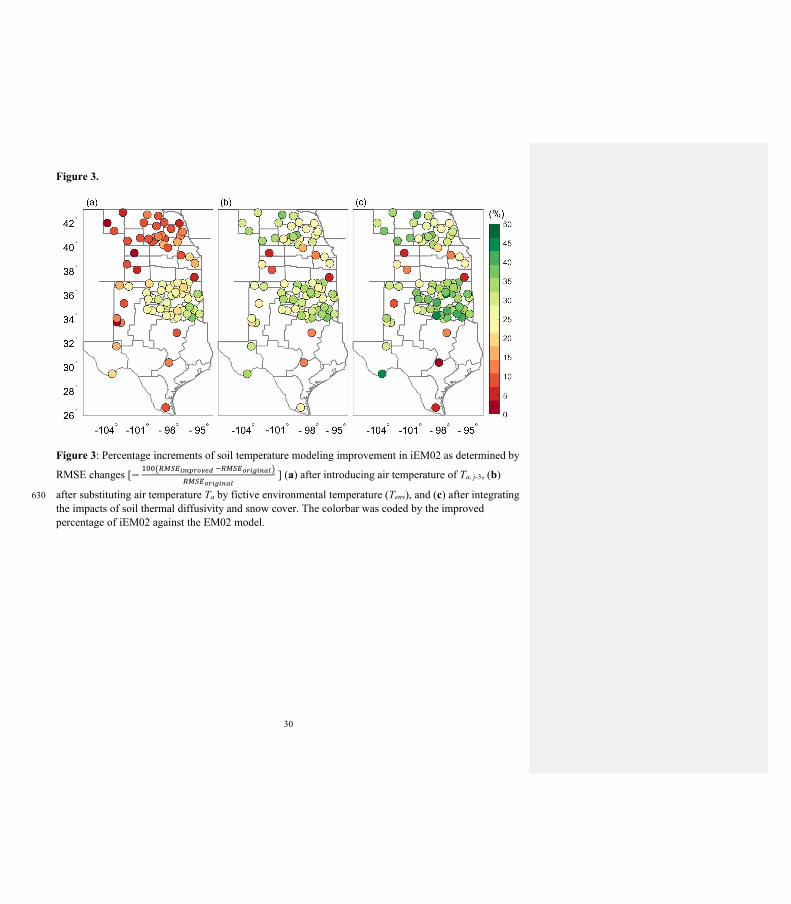
The iEM02 was evaluated from 2015 to 2019 for 87 weather stations. Soil temperature modeling using

different soil textures was improved in different ways in the iEM02 model (Fig. 3). The improvement of

soil temperature modeling indicated by relative RMSE changes was different across sites. The weather 225

stations located in NE and KS as well as TX showed less improvement by introducing the air

temperature of Ta, j-3 compared to OK (Fig. 3a). The soil types in OK are more clay and silt compared to

NE and KS (Fig. 1). However, the improvement by using the fictive environmental temperature was

12

significant in northern areas of NE and KS (sandy soil) but not in the southern area of OK and part of

TX (clay and silt soil) (Fig. 3b). Overall, latitude-dominated air temperature should play a role in 230

improving estimated soil temperature. Most of the 87 stations achieved a 15% to 40% improvement in

simulated soil temperature by introducing air temperature Ta, j-3 and replacing Ta with Tenv. This

improvement was in agreement with a previous study (Dolschak et al., 2015). By incorporating changes

in soil moisture and daily snow depth, additional improvements in soil temperature simulation of up to

50% could be achieved (Fig. 3c) compared to the original model EM02. It should be noted that there 235

were fewer stations available in KS and TX compared to NE and OK. Overall, integrating snow cover

and soil moisture data in iEM02 improved the simulated soil temperature (Fig. 3). The daily soil

temperature modeling could be further improved if high-resolution (e.g., 30 m and daily) satellite-based

soil moisture/snow cover products become available, for example, products based on the SMAP or

Sentinel satellites (Das et al., 2019). 240

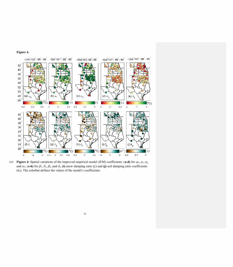
3.2 iEM02’s parameters

The parameters described in iEM02 for each weather station are indicative of soil temperature

sensitivities for each independent variable in Eq. (2) although strictly speaking, they are not

mathematical sensitivities (Fig. 4 & Table A2). For Tenv, the current day Tenv was the most weighted as 245

expected (Fig. 4a). The parameters of Tenv for the prior day 1 to day 3 were relatively weak in terms of

absolute magnitudes due to autoregression properties in the soil temperature (Figs. 4b-d). Interestingly,

in the iEM02 model, the prior day 2 was negatively associated with soil temperature (Fig. 4c) which

cannot be interpreted by soil physical processes but in a more autoregressive sense in which the soil

Deleted: 250

13

temperature signals are superimposed. The periodic property embedded in iEM02 was two low-

frequency components (semi-annual and annual signals). Obviously, the annual signal strength

indicated by b1 and d1 was one-order stronger than the semi-annual signal strengths in soil temperature

(Fig. 4e-h). The result also suggested the strong b1 and d1 spatial contexts of the northern region (e.g., in

Nebraska and Kansas) were differently weighted from those in the southern region (e.g., in Oklahoma 255

and Texas). For the snow damping factor, the snow cover had a larger impact on soil temperature in the

northern region when compared to the southern region (Fig. 4i). However, the soil damping ratio factor

was relatively evenly distributed (Fig. 4j).

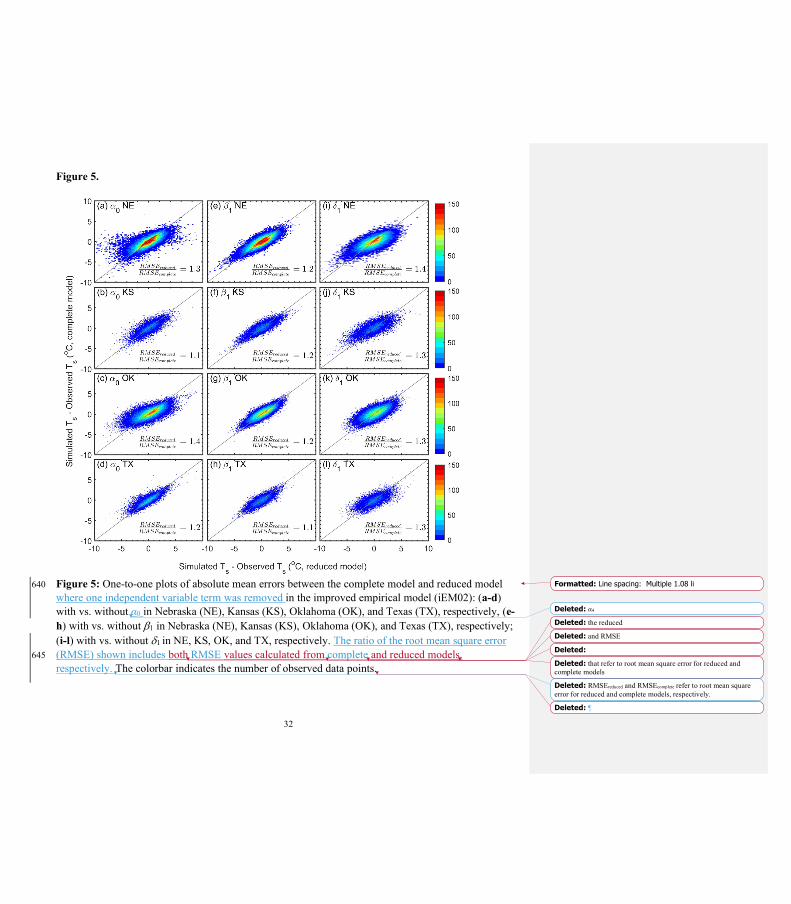
RMSE performance is shown in Figure 5 when the iEM02 was a complete model vs. the reduced model

iEM02 where one independent variable term from the complete model was removed. When removing 260

any one independent variable, the modeled soil temperature RMSE increased from 110% to 130% (Fig.

5), indicating a 20% rise in RMSE. Specifically, the iEM02 model performance decreased (i.e., RMSE

increased from 0.1 to 0.4oC) when the a0 term was removed (Fig. 5, a-d). Unlike a0, removing the b1

term was not as sensitive and gave an increase of 0.1-0.2oC RMSE on average for all states in the region

(Fig. 5, e-h). However, it is clear that the iEM02 model was most sensitive to d1. With the removal of d1 265

from the complete iEM02 model, the RMSE increased 0.3-0.4oC for all four states (Fig. 5, i-l). Due to

the location-dependency of the above coefficients, further spatial interpolation of the iEM02 model

would be beneficial to predict soil temperature for irrigated agricultural areas without weather stations

in the U.S. Great Plains and to improve water and crop management modeling.

270

3.3 Spatial and temporal modeling performance

Formatted: Font color: Text 1

Formatted: Font color: Text 1

Deleted: drop

14

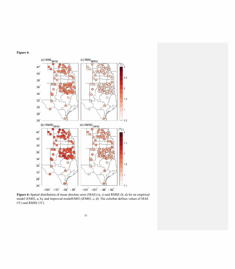
A graphical summary of how closely the modeled soil temperature agreed with the observed soil

temperature for each weather station is shown in Figure 6. Daily Ts estimated in the iEM02 model

outperformed that in the original EM02 model for all 87 weather stations. For example, both MAE and 275

RMSE were decreased on average by 0.6oC when the iEM02 model was used to estimate Ts.

Individually, the improved model showed a less than 1.6oC RMSE for any individual station but 16% of

the stations had larger than 2oC RMSE in the original EM02. In addition, we compared the performance

of iEM02 against a recent energy-balance model (Chalhoub et al., 2017). Our prediction of Ts was

improved by 1.2oC RMSE compared to the energy-balance model (not shown). 280

Spatial distributions of RMSE showed that the majority of weather stations had better performance in

Oklahoma with a mean RMSE of 1.9 and 1.1oC for EM02 and iEM02, respectively, whereas Nebraska

had a RMSE of 2.1 and 1.3oC for EM02 and iEM02, respectively. The different modeling performance

was associated with the soil heat transport process and how frequent snowfall could be observed in 285

Nebraska and Oklahoma. Similar results were presented in a recent study by Huang et al. (2017). On the

other hand, the high quality of weather data from the Oklahoma Mesonet considered to be the "gold

standard" for the statewide weather network (Lin et al., 2016) thus ensured quality of both model

calibrations and observed soil temperature in Oklahoma.

290

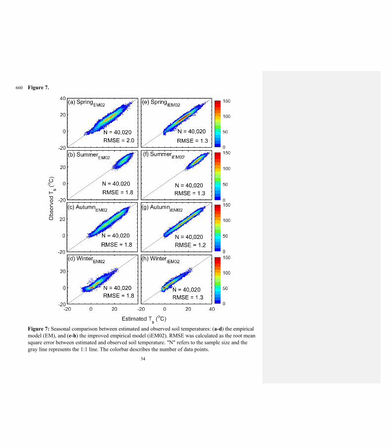
Seasonal Ts indicated that iEM02 modeling was mostly improved in the spring season from 2oC to

1.3oC RMSE (Fig. 7a) but the original model EM02 showed the uncertainty was in good agreement

with the performance achieved in Plauborg (2002). All other seasons were improved in similar ways

Deleted: (

Deleted: , 295 Deleted: )

15

from 1.8oC to 1.2 or 1.3oC RMSE. The improvement for all seasons could be attributed to introducing

soil diffusivity, which changed with daily soil moisture and snow cover, and this affected the soil

thermal conductivity (Rankinen et al., 2004; Zhang, 2005). Moreover, although modeling wintertime

soil temperature improved from 1.8oC to 1.3oC RMSE, which was the same as in the summer (Fig. 7), 300

the soil temperature located in more frequent snow-covered states (e.g., Nebraska and Kansas), was

better improved when Tenv and snow depth were introduced into the model. Our findings confirmed

those reported by Rankinen et al. (2004) and Dutta et al. (2018).

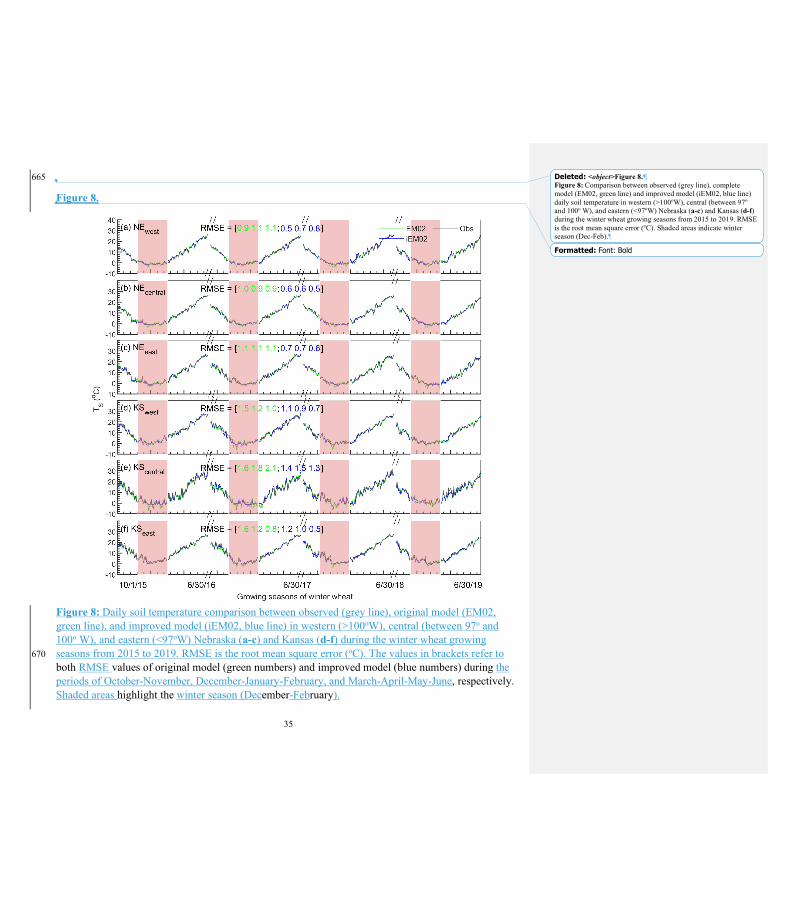
Since precipitation gradients exist in the U.S. Great Plains from western to eastern regions (Evett et al., 305

2020), three subregions were classified for each state as western (100oW towards west), central

(between 97o and 100oW), and eastern (97oW towards east). Figure 8 displays the time series of EM02

modeled, iEM02 modeled, and observed soil temperatures only covering winter wheat growing seasons

(October 1 to June 30) for four growing seasons from 2015 to 2019 (validation periods) in Nebraska and

Kansas. All subregions in Nebraska and Kansas showed improvement when using the iEM02 model 310

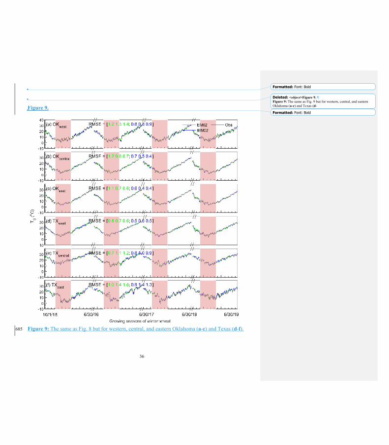
(Fig. 8). Similarly, the iEM02 improved the RMSE during four growing seasons in Oklahoma and

Texas (Fig. 9). The EM02 model had the best performance in Oklahoma with a mean RMSE of 1.0oC,

while the mean RMSE in Kansas was 1.4oC in EM02. Soil temperatures estimated by iEM02 had

approximately a 0.3 to 1.4oC RMSE (Figs. 8 and 9). In addition, larger improvements by iEM02 were

observed in most subregions during wintertime, which would be beneficial for modeling winter wheat 315

yields and potential yields (Persson et al., 2017).

Deleted: (Rankinen et al., 2004; Dutta et al., 2018).

Deleted: accurately

16

4. Conclusion 320

The primary intention of this work was to develop an improved soil temperature model for the U.S.

Great Plains that can predict soil temperature by using common weather station variables as inputs. The

improved empirical model (iEM02) integrated soil thermal diffusivity and snow cover factors, and they

significantly improved the estimate of soil temperature for 87 weather stations in the U.S. Great Plains

that were studied. Specifically, after incorporating changes in soil moisture and daily snow depth, the 325

improved model showed a near 50% gain in performance in terms of RMSE decrease compared to the

original model. The value of RMSE across 87 stations was 0.6oC lower on average than the original

model from 2015 to 2019. We concluded that the iEM02 model can better estimate soil temperature at

the surface soil layer where most hydrological and biological processes occur. Both seasonal and spatial

improvements made in the improved model demonstrated the robustness of the iEM02 model, 330

suggesting this improved model can provide a reliable simulation of soil temperature to use in modeling

hydrological process and crop production in the U.S. Great Plains.

Deleted: in the improved model

Deleted: better 335

17

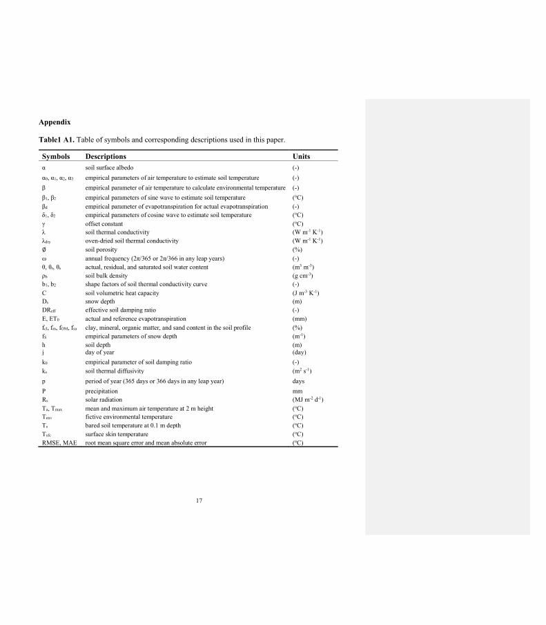
Appendix

Table1 A1. Table of symbols and corresponding descriptions used in this paper.

Symbols Descriptions Units α soil surface albedo (-) α0, α1, α2, α3 empirical parameters of air temperature to estimate soil temperature (-) β empirical parameter of air temperature to calculate environmental temperature (-) β1, β2 empirical parameters of sine wave to estimate soil temperature (oC) βd empirical parameter of evapotranspiration for actual evapotranspiration (-) δ1, δ2 empirical parameters of cosine wave to estimate soil temperature (oC) γ offset constant (oC) λ soil thermal conductivity (W m-1 K-1) λdry oven-dried soil thermal conductivity (W m-1 K-1) ∅ soil porosity (%) ω annual frequency (2π/365 or 2π/366 in any leap years) (-) θ, θr, θs actual, residual, and saturated soil water content (m3 m-3) ρb soil bulk density (g cm-3) b1, b2 shape factors of soil thermal conductivity curve (-) C soil volumetric heat capacity (J m-3 K-1) Ds snow depth (m) DReff effective soil damping ratio (-) E, ET0 actual and reference evapotranspiration (mm) fcl, fm, fOM, fsa clay, mineral, organic matter, and sand content in the soil profile (%) fS empirical parameters of snow depth (m-1) h soil depth (m) j day of year (day) k0 empirical parameter of soil damping ratio (-) ks soil thermal diffusivity (m2 s-1) p period of year (365 days or 366 days in any leap year) days P precipitation mm Rs solar radiation (MJ m-2 d-1) Ta, Tmax mean and maximum air temperature at 2 m height (oC) Tenv fictive environmental temperature (oC) Ts bared soil temperature at 0.1 m depth (oC) Tsfc surface skin temperature (oC) RMSE, MAE root mean square error and mean absolute error (oC)

18

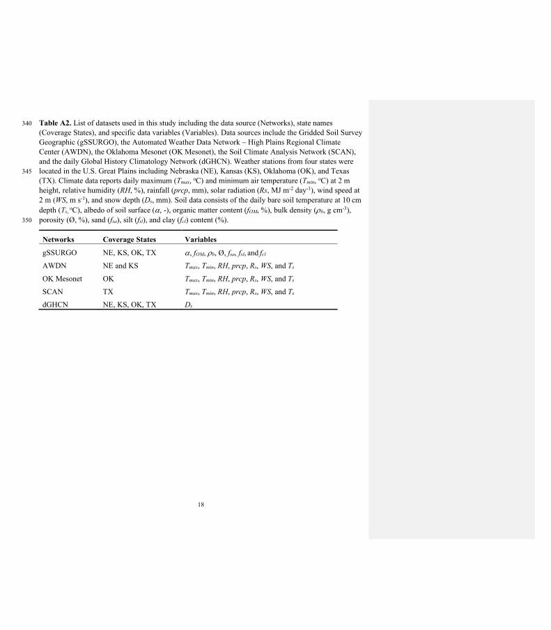
Table A2. List of datasets used in this study including the data source (Networks), state names 340 (Coverage States), and specific data variables (Variables). Data sources include the Gridded Soil Survey Geographic (gSSURGO), the Automated Weather Data Network – High Plains Regional Climate Center (AWDN), the Oklahoma Mesonet (OK Mesonet), the Soil Climate Analysis Network (SCAN), and the daily Global History Climatology Network (dGHCN). Weather stations from four states were located in the U.S. Great Plains including Nebraska (NE), Kansas (KS), Oklahoma (OK), and Texas 345 (TX). Climate data reports daily maximum (Tmax, oC) and minimum air temperature (Tmin, oC) at 2 m height, relative humidity (RH, %), rainfall (prcp, mm), solar radiation (Rs, MJ m-2 day-1), wind speed at 2 m (WS, m s-1), and snow depth (Ds, mm). Soil data consists of the daily bare soil temperature at 10 cm depth (Ts, oC), albedo of soil surface (a, -), organic matter content (fOM, %), bulk density (rb, g cm-3), porosity (Ø, %), sand (fsa), silt (fsl), and clay (fcl) content (%). 350

Networks Coverage States Variables

gSSURGO NE, KS, OK, TX a, fOM, rb, Ø, fsa, fsl, and fcl

AWDN NE and KS Tmax, Tmin, RH, prcp, Rs, WS, and Ts

OK Mesonet OK Tmax, Tmin, RH, prcp, Rs, WS, and Ts

SCAN TX Tmax, Tmin, RH, prcp, Rs, WS, and Ts

dGHCN NE, KS, OK, TX Ds

19

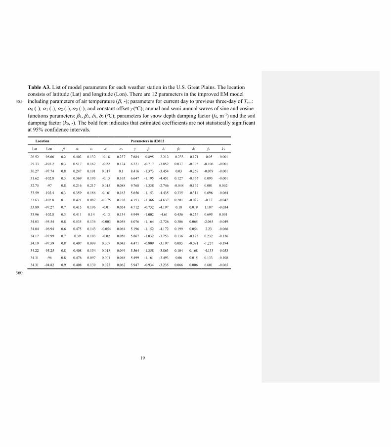
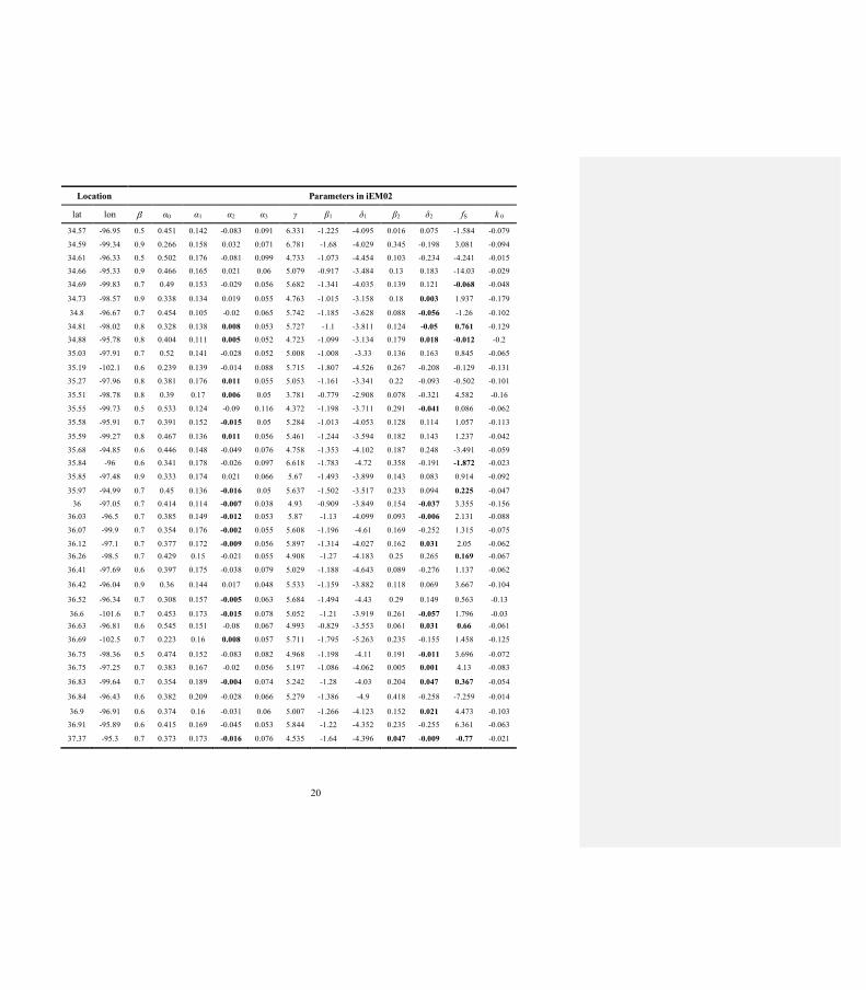
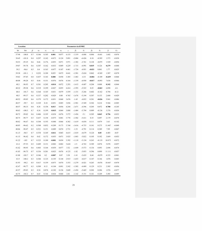
Table A3. List of model parameters for each weather station in the U.S. Great Plains. The location consists of latitude (Lat) and longitude (Lon). There are 12 parameters in the improved EM model including parameters of air temperature (b, -); parameters for current day to previous three-day of Tenv: 355 a0 (-), a1 (-), a2 (-), a3 (-), and constant offset γ (oC); annual and semi-annual waves of sine and cosine functions parameters: b1, b2, d1, d2 (oC); parameters for snow depth damping factor (fS, m-1) and the soil damping factor (k0, -). The bold font indicates that estimated coefficients are not statistically significant at 95% confidence intervals.

Location Parameters in iEM02

Lat Lon b α0 α1 α2 α3 γ β1 δ1 β2 δ2 fS k 0 26.52 -98.06 0.2 0.402 0.132 -0.18 0.237 7.684 -0.895 -2.212 -0.233 -0.171 -0.05 -0.001

29.33 -103.2 0.3 0.517 0.162 -0.22 0.174 6.221 -0.717 -3.852 0.037 -0.398 -0.106 -0.001

30.27 -97.74 0.8 0.247 0.191 0.017 0.1 8.416 -1.373 -3.454 0.03 -0.269 -0.079 -0.001

31.62 -102.8 0.3 0.369 0.193 -0.13 0.165 6.647 -1.195 -4.451 0.127 -0.365 0.093 -0.001

32.75 -97 0.8 0.216 0.217 0.015 0.088 9.768 -1.338 -2.746 -0.048 -0.167 0.001 0.002

33.59 -102.4 0.3 0.359 0.186 -0.161 0.163 5.656 -1.153 -4.435 0.335 -0.314 0.696 -0.064

33.63 -102.8 0.1 0.421 0.087 -0.175 0.228 4.153 -1.366 -4.637 0.201 -0.077 -0.27 -0.047

33.89 -97.27 0.7 0.415 0.196 -0.01 0.054 4.712 -0.732 -4.197 0.18 0.019 1.187 -0.034

33.96 -102.8 0.3 0.411 0.14 -0.13 0.134 4.949 -1.002 -4.61 0.456 -0.256 0.695 0.001

34.03 -95.54 0.8 0.535 0.136 -0.003 0.058 4.076 -1.164 -2.726 0.306 0.065 -2.045 -0.049

34.04 -96.94 0.6 0.475 0.143 -0.054 0.064 5.196 -1.152 -4.172 0.199 0.054 2.23 -0.066

34.17 -97.99 0.7 0.39 0.103 -0.02 0.056 5.867 -1.032 -3.753 0.136 -0.173 0.232 -0.156

34.19 -97.59 0.8 0.407 0.099 0.009 0.043 4.471 -0.809 -3.197 0.085 -0.091 -1.257 -0.194

34.22 -95.25 0.8 0.408 0.154 0.018 0.049 5.564 -1.358 -3.863 0.104 0.168 -4.133 -0.053

34.31 -96 0.8 0.476 0.097 0.001 0.048 5.499 -1.161 -3.493 0.06 0.015 0.133 -0.108

34.31 -94.82 0.9 0.408 0.139 0.025 0.062 5.947 -0.934 -3.235 0.066 0.006 6.601 -0.065

360

20

Location Parameters in iEM02

lat lon b α0 α1 α2 α3 γ β1 δ1 β2 δ2 fS k 0

34.57 -96.95 0.5 0.451 0.142 -0.083 0.091 6.331 -1.225 -4.095 0.016 0.075 -1.584 -0.079

34.59 -99.34 0.9 0.266 0.158 0.032 0.071 6.781 -1.68 -4.029 0.345 -0.198 3.081 -0.094

34.61 -96.33 0.5 0.502 0.176 -0.081 0.099 4.733 -1.073 -4.454 0.103 -0.234 -4.241 -0.015 34.66 -95.33 0.9 0.466 0.165 0.021 0.06 5.079 -0.917 -3.484 0.13 0.183 -14.03 -0.029

34.69 -99.83 0.7 0.49 0.153 -0.029 0.056 5.682 -1.341 -4.035 0.139 0.121 -0.068 -0.048

34.73 -98.57 0.9 0.338 0.134 0.019 0.055 4.763 -1.015 -3.158 0.18 0.003 1.937 -0.179

34.8 -96.67 0.7 0.454 0.105 -0.02 0.065 5.742 -1.185 -3.628 0.088 -0.056 -1.26 -0.102

34.81 -98.02 0.8 0.328 0.138 0.008 0.053 5.727 -1.1 -3.811 0.124 -0.05 0.761 -0.129 34.88 -95.78 0.8 0.404 0.111 0.005 0.052 4.723 -1.099 -3.134 0.179 0.018 -0.012 -0.2

35.03 -97.91 0.7 0.52 0.141 -0.028 0.052 5.008 -1.008 -3.33 0.136 0.163 0.845 -0.065

35.19 -102.1 0.6 0.239 0.139 -0.014 0.088 5.715 -1.807 -4.526 0.267 -0.208 -0.129 -0.131

35.27 -97.96 0.8 0.381 0.176 0.011 0.055 5.053 -1.161 -3.341 0.22 -0.093 -0.502 -0.101

35.51 -98.78 0.8 0.39 0.17 0.006 0.05 3.781 -0.779 -2.908 0.078 -0.321 4.582 -0.16

35.55 -99.73 0.5 0.533 0.124 -0.09 0.116 4.372 -1.198 -3.711 0.291 -0.041 0.086 -0.062

35.58 -95.91 0.7 0.391 0.152 -0.015 0.05 5.284 -1.013 -4.053 0.128 0.114 1.057 -0.113

35.59 -99.27 0.8 0.467 0.136 0.011 0.056 5.461 -1.244 -3.594 0.182 0.143 1.237 -0.042

35.68 -94.85 0.6 0.446 0.148 -0.049 0.076 4.758 -1.353 -4.102 0.187 0.248 -3.491 -0.059 35.84 -96 0.6 0.341 0.178 -0.026 0.097 6.618 -1.783 -4.72 0.358 -0.191 -1.872 -0.023

35.85 -97.48 0.9 0.333 0.174 0.021 0.066 5.67 -1.493 -3.899 0.143 0.083 0.914 -0.092

35.97 -94.99 0.7 0.45 0.136 -0.016 0.05 5.637 -1.502 -3.517 0.233 0.094 0.225 -0.047 36 -97.05 0.7 0.414 0.114 -0.007 0.038 4.93 -0.909 -3.849 0.154 -0.037 3.355 -0.156

36.03 -96.5 0.7 0.385 0.149 -0.012 0.053 5.87 -1.13 -4.099 0.093 -0.006 2.131 -0.088

36.07 -99.9 0.7 0.354 0.176 -0.002 0.055 5.608 -1.196 -4.61 0.169 -0.252 1.315 -0.075

36.12 -97.1 0.7 0.377 0.172 -0.009 0.056 5.897 -1.314 -4.027 0.162 0.031 2.05 -0.062 36.26 -98.5 0.7 0.429 0.15 -0.021 0.055 4.908 -1.27 -4.183 0.25 0.265 0.169 -0.067

36.41 -97.69 0.6 0.397 0.175 -0.038 0.079 5.029 -1.188 -4.643 0.089 -0.276 1.137 -0.062

36.42 -96.04 0.9 0.36 0.144 0.017 0.048 5.533 -1.159 -3.882 0.118 0.069 3.667 -0.104

36.52 -96.34 0.7 0.308 0.157 -0.005 0.063 5.684 -1.494 -4.43 0.29 0.149 0.563 -0.13

36.6 -101.6 0.7 0.453 0.173 -0.015 0.078 5.052 -1.21 -3.919 0.261 -0.057 1.796 -0.03 36.63 -96.81 0.6 0.545 0.151 -0.08 0.067 4.993 -0.829 -3.553 0.061 0.031 0.66 -0.061

36.69 -102.5 0.7 0.223 0.16 0.008 0.057 5.711 -1.795 -5.263 0.235 -0.155 1.458 -0.125

36.75 -98.36 0.5 0.474 0.152 -0.083 0.082 4.968 -1.198 -4.11 0.191 -0.011 3.696 -0.072 36.75 -97.25 0.7 0.383 0.167 -0.02 0.056 5.197 -1.086 -4.062 0.005 0.001 4.13 -0.083

36.83 -99.64 0.7 0.354 0.189 -0.004 0.074 5.242 -1.28 -4.03 0.204 0.047 0.367 -0.054

36.84 -96.43 0.6 0.382 0.209 -0.028 0.066 5.279 -1.386 -4.9 0.418 -0.258 -7.259 -0.014

36.9 -96.91 0.6 0.374 0.16 -0.031 0.06 5.007 -1.266 -4.123 0.152 0.021 4.473 -0.103 36.91 -95.89 0.6 0.415 0.169 -0.045 0.053 5.844 -1.22 -4.352 0.235 -0.255 6.361 -0.063

37.37 -95.3 0.7 0.373 0.173 -0.016 0.076 4.535 -1.64 -4.396 0.047 -0.009 -0.77 -0.021

21

Location Parameters in iEM02

lat lon b α0 α1 α2 α3 γ β1 δ1 β2 δ2 fS k 0 37.98 -100.8 0.7 0.346 0.185 0.001 0.077 4.153 -1.319 -4.886 0.084 -0.441 1.602 -0.074

38.45 -101.8 0.4 0.297 0.142 -0.073 0.124 5.091 -2.004 -6.426 0.18 -0.585 1.573 -0.038

38.53 -95.25 0.6 0.46 0.176 -0.053 0.071 3.971 -1.302 -3.761 0.128 -0.075 1.529 -0.054

39.07 -95.78 0.6 0.387 0.162 -0.033 0.089 4.229 -1.715 -4.991 0.019 0.126 0.279 -0.048

39.2 -96.6 0.5 0.4 0.163 -0.077 0.107 4.461 -1.724 -4.951 -0.021 0.081 1.77 -0.025

39.38 -101.1 1 0.252 0.188 0.055 0.075 4.641 -1.501 -5.624 0.062 -0.369 1.507 -0.078

39.82 -97.85 0.8 0.437 0.182 0.008 0.058 3.385 -1.482 -4.33 -0.004 -0.109 -0.429 -0.068

40.08 -98.28 0.5 0.44 0.151 -0.076 0.076 4.164 -1.339 -4.958 -0.017 -0.093 7.636 -0.046

40.3 -96.93 0.7 0.381 0.205 -0.014 0.072 3.293 -1.615 -4.407 0.204 0.088 0.342 -0.064

40.32 -99.38 0.6 0.319 0.199 -0.027 0.055 4.414 -1.593 -5.523 0.25 -0.063 6.898 -0.1

40.4 -101.7 0.6 0.364 0.145 -0.031 0.079 3.559 -1.151 -5.266 0.402 -0.162 8.794 -0.12

40.5 -99.37 0.6 0.337 0.202 -0.029 0.08 4.765 -1.676 -5.194 0.307 0.153 2.688 -0.029

40.52 -99.05 0.6 0.379 0.172 -0.031 0.068 3.676 -1.45 -4.852 0.281 -0.026 5.941 -0.086

40.57 -99.7 0.5 0.329 0.18 -0.051 0.085 3.856 -1.901 -5.549 0.302 0.214 9.566 -0.085

40.57 -98.15 0.8 0.28 0.158 0.013 0.056 4.244 -1.671 -4.596 0.205 0.072 0.708 -0.245

40.63 -100.5 0.7 0.36 0.199 -0.015 0.064 3.888 -1.484 -5.794 0.089 -0.136 3.376 -0.054

40.72 -99.02 0.6 0.406 0.195 -0.034 0.076 3.572 -1.456 -5.1 0.205 0.043 0.756 -0.032

40.75 -98.77 0.5 0.437 0.158 -0.075 0.081 3.778 -1.502 -5.411 0.35 0.097 2.179 -0.078

40.82 -96.67 0.6 0.384 0.193 -0.048 0.066 4.302 -1.619 -4.854 0.111 0.079 3.63 -0.102

40.85 -96.62 0.2 0.588 0.032 -0.209 0.173 3.744 -1.616 -4.753 0.141 0.275 11.447 -0.048

40.86 -98.47 0.5 0.521 0.151 -0.089 0.074 2.731 -1.53 -4.791 0.114 0.309 7.99 -0.067

41.15 -96.5 0.7 0.354 0.169 -0.011 0.065 4.615 -1.819 -4.679 0.124 0.05 4.403 -0.07

41.15 -96.42 0.6 0.42 0.172 -0.055 0.071 3.925 -1.883 -5.022 0.105 0.102 3.669 -0.053

41.22 -103 0.7 0.323 0.188 -0.001 0.054 3.392 -1.118 -5.154 0.263 -0.119 10.875 -0.072

41.4 -97.53 0.5 0.489 0.131 -0.082 0.082 3.624 -1.5 -4.763 0.389 0.074 5.878 -0.057

41.62 -98.95 0.6 0.403 0.164 -0.039 0.077 3.52 -1.649 -5.573 0.136 0.093 2.696 -0.074

41.85 -96.75 0.7 0.336 0.201 -0.025 0.076 4.125 -1.82 -5.053 0.296 0.099 11.111 -0.057

41.88 -103.7 0.7 0.346 0.2 -0.007 0.07 3.58 -1.41 -5.435 0.44 -0.079 4.335 -0.061

41.9 -100.2 0.3 0.548 0.125 -0.195 0.144 2.915 -1.653 -4.817 0.187 0.146 1.078 -0.043

41.93 -98.2 0.5 0.417 0.159 -0.073 0.074 3.353 -1.279 -4.421 0.243 -0.076 10.447 -0.078

42.47 -98.77 0.5 0.509 0.13 -0.104 0.091 3.542 -1.505 -4.489 0.129 0.231 2.505 -0.056

42.57 -99.83 0.3 0.54 0.074 -0.182 0.156 3.049 -1.454 -5.465 0.202 0.286 1.976 -0.077

42.75 -102.2 0.7 0.43 0.144 -0.024 0.068 2.82 -1.142 -5.151 0.141 0.249 3.492 -0.089

22

Code availability

MATLAB code is available upon request. 365

Data availability

Data used in this study are available by the links above (material and methods).

Author contribution 370

HZ and XL designed the experiments, conducted simulations, analyzed the data, and wrote the manuscript. NW helped data analysis, result interpretation, and discussion. MBK and GFS provided suggestions and discussion, wrote the manuscripts, and revised the manuscript.

Competing interests 375

The authors declare that they have no conflict of interest.

Acknowledgements This study was supported in part by the U.S. Department of Agriculture, National Institute of Food and Agriculture (grant no. 2016-68007- 25066 and grant no. 2016-68007- 25066) and the Kansas Crop 380 Improvement Association, the U.S. Department of Agriculture National Institute of Food and Agriculture, Hatch project 1018005. The contribution number of this manuscript is 20-252-J. We appreciated Dr. Gerard Kluitenberg and Dr. Jesse Tack at Kansas State University for providing helpful suggestions to improve the quality of paper. We thank Dallas Staley for her outstanding contribution in editing and finalizing the paper. Her work continues to be at the highest professional level. 385

Deleted: HD

23

References

Abu-Hamdeh, N. H.: Thermal Properties of Soils as affected by Density and Water Content, Biosystems Engineering, 86, 425 97-102, 10.1016/s1537-5110(03)00112-0, 2003.

Allen, R. G., Pereira, L. S., Raes, D., and Smith, M.: Crop evapotranspiration-Guidelines for computing crop water requirements-FAO Irrigation and drainage paper 56, Fao, Rome, 300, D05109, 1998.

Araghi, A., Mousavi-Baygi, M., Adamowski, J., Martinez, C., and van der Ploeg, M.: Forecasting soil temperature based on surface air temperature using a wavelet artificial neural network, Meteorological Applications, 24, 603-611, 430 10.1002/met.1661, 2017.

Badache, M., Eslami-Nejad, P., Ouzzane, M., Aidoun, Z., and Lamarche, L.: A new modeling approach for improved ground temperature profile determination, Renewable Energy, 85, 436-444, 10.1016/j.renene.2015.06.020, 2016.

Badía, D., López-García, S., Martí, C., Ortíz-Perpiñá, O., Girona-García, A., and Casanova-Gascón, J.: Burn effects on soil properties associated to heat transfer under contrasting moisture content, Science of the Total Environment, 601, 1119-435 1128, 2017.

Bergjord, A. K., Bonesmo, H., and Skjelvåg, A. O.: Modelling the course of frost tolerance in winter wheat, European Journal of Agronomy, 28, 321-330, 10.1016/j.eja.2007.10.002, 2008.

Bittelli, M., Ventura, F., Campbell, G. S., Snyder, R. L., Gallegati, F., and Pisa, P. R.: Coupling of heat, water vapor, and liquid water fluxes to compute evaporation in bare soils, Journal of Hydrology, 362, 191-205, 440 10.1016/j.jhydrol.2008.08.014, 2008.

Brock, F. V. and Crawford, K. C.: The Oklahoma Mesonet_ A Technical Overview, Journal of Atmospheric and Oceanic Technology, 1995.

Chalhoub, M., Bernier, M., Coquet, Y., and Philippe, M.: A simple heat and moisture transfer model to predict ground temperature for shallow ground heat exchangers, Renewable Energy, 103, 295-307, 10.1016/j.renene.2016.11.027, 2017. 445

Das, N. N., Entekhabi, D., Dunbar, R. S., Chaubell, M. J., Colliander, A., Yueh, S., Jagdhuber, T., Chen, F., Crow, W., and O'Neill, P. E.: The SMAP and Copernicus Sentinel 1A/B microwave active-passive high resolution surface soil moisture product, Remote Sensing of Environment, 233, 111380, 2019.

Dhungel, R., Aiken, R., Evett, S. R., Colaizzi, P. D., Marek, G., Moorhead, J. E., Baumhardt, R. L., Brauer, D., Kutikoff, S., and Lin, X.: Energy Imbalance and Evapotranspiration Hysteresis under an Advective Environment: Evidence from 450 Lysimeter, Eddy Covariance, and Energy Balance Modelling, Geophysical Research Letters, e2020GL091203, 2021.

Dirmeyer, P. A. and Norton, H. E.: Indications of surface and sub-surface hydrologic properties from SMAP soil moisture retrievals, Hydrology, 5, 36, 2018.

Dolschak, K., Gartner, K., and Berger, T. W.: A new approach to predict soil temperature under vegetated surfaces, Modeling earth systems and environment, 1, 32, 2015. 455

Dutta, B., Grant, B. B., Congreves, K. A., Smith, W. N., Wagner-Riddle, C., VanderZaag, A. C., Tenuta, M., and Desjardins, R. L.: Characterising effects of management practices, snow cover, and soil texture on soil temperature: Model development in DNDC, Biosystems Engineering, 168, 54-72, 10.1016/j.biosystemseng.2017.02.001, 2018.

Evett, S. R., Colaizzi, P. D., Lamm, F. R., O’Shaughnessy, S. A., Heeren, D. M., Trout, T. J., Kranz, W. L., and Lin, X.: Past, present, and future of irrigation on the US Great Plains, Transactions of the ASABE, 63, 703-729, 2020. 460

Goulden, M., Wofsy, S., Harden, J., Trumbore, S. E., Crill, P., Gower, S., Fries, T., Daube, B., Fan, S.-M., and Sutton, D.: Sensitivity of boreal forest carbon balance to soil thaw, Science, 279, 214-217, 1998.

Gupta, S. C., Radke, J. K., Swan, J. B., and Moncrief, J. F.: Predicting soil temperature under a ridge-furrow system in the U.S. Corm Belt, Soil& Tillage Research, 18, 145-165, 1990.

Haacker, E. M., Cotterman, K. A., Smidt, S. J., Kendall, A. D., and Hyndman, D. W.: Effects of management areas, drought, 465 and commodity prices on groundwater decline patterns across the High Plains Aquifer, Agricultural Water Management, 218, 259-273, 2019.

Hillel, D.: Environmental soil physics: Fundamentals, applications, and environmental considerations, Elsevier1998. Huang, Y., Jiang, J., Ma, S., Ricciuto, D., Hanson, P. J., and Luo, Y.: Soil thermal dynamics, snow cover, and frozen depth

under five temperature treatments in an ombrotrophic bog: Constrained forecast with data assimilation, Journal of 470 Geophysical Research: Biogeosciences, 122, 2046-2063, 10.1002/2016jg003725, 2017.

24

Kang, S., Kim, S., Oh, S., and Lee, D.: Predicting spatial and temporal patterns of soil temperature based on topography, surface cover and air temperature, Forest Ecology and Management, 136, 173-184, 2000.

Kutikoff, S., Lin, X., Evett, S. R., Gowda, P., Brauer, D., Moorhead, J., Marek, G., Colaizzi, P., Aiken, R., and Xu, L.: Water vapor density and turbulent fluxes from three generations of infrared gas analyzers, Atmospheric Measurement 475 Techniques, 14, 1253-1266, 2021.

Lakshmi, V., Jackson, T. J., and Zehrfuhs, D.: Soil moisture–temperature relationships: results from two field experiments, Hydrological processes, 17, 3041-3057, 2003.

Lembrechts, J. J., Aalto, J., Ashcroft, M. B., De Frenne, P., Kopecky, M., Lenoir, J., Luoto, M., Maclean, I. M. D., Roupsard, O., Fuentes-Lillo, E., Garcia, R. A., Pellissier, L., Pitteloud, C., Alatalo, J. M., Smith, S. W., Bjork, R. G., 480 Muffler, L., Ratier Backes, A., Cesarz, S., Gottschall, F., Okello, J., Urban, J., Plichta, R., Svatek, M., Phartyal, S. S., Wipf, S., Eisenhauer, N., Puscas, M., Turtureanu, P. D., Varlagin, A., Dimarco, R. D., Jump, A. S., Randall, K., Dorrepaal, E., Larson, K., Walz, J., Vitale, L., Svoboda, M., Finger Higgens, R., Halbritter, A. H., Curasi, S. R., Klupar, I., Koontz, A., Pearse, W. D., Simpson, E., Stemkovski, M., Jessen Graae, B., Vedel Sorensen, M., Hoye, T. T., Fernandez Calzado, M. R., Lorite, J., Carbognani, M., Tomaselli, M., Forte, T. G. W., Petraglia, A., Haesen, S., Somers, 485 B., Van Meerbeek, K., Bjorkman, M. P., Hylander, K., Merinero, S., Gharun, M., Buchmann, N., Dolezal, J., Matula, R., Thomas, A. D., Bailey, J. J., Ghosn, D., Kazakis, G., de Pablo, M. A., Kemppinen, J., Niittynen, P., Rew, L., Seipel, T., Larson, C., Speed, J. D. M., Ardo, J., Cannone, N., Guglielmin, M., Malfasi, F., Bader, M. Y., Canessa, R., Stanisci, A., Kreyling, J., Schmeddes, J., Teuber, L., Aschero, V., Ciliak, M., Malis, F., De Smedt, P., Govaert, S., Meeussen, C., Vangansbeke, P., Gigauri, K., Lamprecht, A., Pauli, H., Steinbauer, K., Winkler, M., Ueyama, M., Nunez, M. A., Ursu, 490 T. M., Haider, S., Wedegartner, R. E. M., Smiljanic, M., Trouillier, M., Wilmking, M., Altman, J., Bruna, J., Hederova, L., Macek, M., Man, M., Wild, J., Vittoz, P., Partel, M., Barancok, P., Kanka, R., Kollar, J., Palaj, A., Barros, A., Mazzolari, A. C., Bauters, M., Boeckx, P., Benito Alonso, J. L., Zong, S., Di Cecco, V., Sitkova, Z., Tielborger, K., van den Brink, L., Weigel, R., Homeier, J., Dahlberg, C. J., Medinets, S., Medinets, V., De Boeck, H. J., Portillo-Estrada, M., Verryckt, L. T., Milbau, A., Daskalova, G. N., Thomas, H. J. D., Myers-Smith, I. H., Blonder, B., Stephan, J. G., 495 Descombes, P., Zellweger, F., Frei, E. R., Heinesch, B., Andrews, C., Dick, J., Siebicke, L., Rocha, A., Senior, R. A., Rixen, C., Jimenez, J. J., Boike, J., Pauchard, A., Scholten, T., Scheffers, B., Klinges, D., Basham, E. W., Zhang, J., Zhang, Z., Geron, C., Fazlioglu, F., Candan, O., Sallo Bravo, J., Hrbacek, F., Laska, K., Cremonese, E., Haase, P., Moyano, F. E., Rossi, C., and Nijs, I.: SoilTemp: A global database of near-surface temperature, Glob Chang Biol, 10.1111/gcb.15123, 2020. 500

Liang, L. L., Riveros-Iregui, D. A., Emanuel, R. E., and McGlynn, B. L.: A simple framework to estimate distributed soil temperature from discrete air temperature measurements in data-scarce regions, Journal of Geophysical Research: Atmospheres, 119, 407-417, 10.1002/2013jd020597, 2014.

Lin, X., Pielke Sr, R. A., Mahmood, R., Fiebrich, C. A., and Aiken, R.: Observational evidence of temperature trends at two levels in the surface layer, Atmospheric Chemistry and Physics, 16, 827-841, 10.5194/acp-16-827-2016, 2016. 505

Lin, X., Harrington, J., Ciampitti, I., Gowda, P., Brown, D., and Kisekka, I.: Kansas trends and changes in temperature, precipitation, drought, and frost-free days from the 1890s to 2015, Journal of Contemporary Water Research & Education, 162, 18-30, 2017.

Lu, Y., Lu, S., Horton, R., and Ren, T.: An Empirical Model for Estimating Soil Thermal Conductivity from Texture, Water Content, and Bulk Density, Soil Science Society of America Journal, 78, 1859-1868, 10.2136/sssaj2014.05.0218, 2014. 510

Menne, M. J., Williams Jr, C. N., and Vose, R. S.: The US Historical Climatology Network monthly temperature data, version 2, Bulletin of the American Meteorological Society, 90, 993-1008, 2009.

Meyer, N., Welp, G., and Amelung, W.: The temperature sensitivity (Q10) of soil respiration: controlling factors and spatial prediction at regional scale based on environmental soil classes, Global Biogeochemical Cycles, 32, 306-323, 2018.

Mihalakakou, G., Santamouris, M., Lewis, J., and Asimakopoulos, D.: On the application of the energy balance equation to 515 predict ground temperature profiles, Solar Energy, 60, 181-190, 1997.

Miller, K., Luck, J., Heeren, D. M., Lo, T., Martin, D., and Barker, J.: A geospatial variable rate irrigation control scenario evaluation methodology based on mining root zone available water capacity, Precision agriculture, 19, 666-683, 2018.

Nagare, R. M., Schincariol, R. A., Quinton, W. L., and Hayashi, M.: Effects of freezing on soil temperature, freezing front propagation and moisture redistribution in peat: laboratory investigations, Hydrology and Earth System Sciences, 16, 520 501-515, 2012.

25

Nobel, P. S. and Geller, G. N.: Temperature modelling of wet and dry desert soils, The Journal of Ecology, 247-258, 1987. Onwuka, B. and Mang, B.: Effects of soil temperature on some soil properties and plant growth, Adv. Plants Agric. Res, 8,

34-37, 2018. Paulsen, G. M. and Heyne, E. G.: Grain production of winter wheat after spring freeze injury, Agronomy Journal, 75, 1983. 525 Persson, T. and Wirén, A.: Nitrogen mineralization and potential nitrification at different depths in acid forest soils, in:

Nutrient uptake and cycling in forest ecosystems, Springer, 55-65, 1995. Persson, T., Bergjord Olsen, A. K., Nkurunziza, L., Sindhöj, E., and Eckersten, H.: Estimation of Crown Temperature of

Winter Wheat and the Effect on Simulation of Frost Tolerance, Journal of Agronomy and Crop Science, 203, 161-176, 10.1111/jac.12187, 2017. 530

Plauborg, F.: Simple model for 10 cm soil temperature in different soilswith short grass, European Journal of Agronomy, 17, 173-179, 2002.

Qi, J., Zhang, X., and Cosh, M. H.: Modeling soil temperature in a temperate region: A comparison between empirical and physically based methods in SWAT, Ecological Engineering, 129, 134-143, 2019.

Qi, J., Li, S., Li, Q., Xing, Z., Bourque, C. P.-A., and Meng, F.-R.: A new soil-temperature module for SWAT application in 535 regions with seasonal snow cover, Journal of Hydrology, 538, 863-877, 2016.

Rankinen, K., Karvonen, T., and Butterfield, D.: A simple model for predicting soil temperature in snow-covered and seasonally frozen soil: model description and testing, Hydrology and Earth System Sciences, 8, 706-716, 10.5194/hess-8-706-2004, 2004.

Rosenberg, N. J., Blad, B. L., and Verma, S. B.: Microclimate: the biological environment, John Wiley & Sons1983. 540 Smith, K. A.: Soil and environmental analysis: physical methods, revised, and expanded, CRC Press 2000. Soong, J. L., Phillips, C. L., Ledna, C., Koven, C. D., and Torn, M. S.: CMIP5 models predict rapid and deep soil warming

over the 21st century, Journal of Geophysical Research: Biogeosciences, 125, e2019JG005266, 2020. Stone, P., Sorensen, I., and Jamieson, P.: Effect of soil temperature on phenology, canopy development, biomass and yield of

maize in a cool-temperate climate, Field crops research, 63, 169-178, 1999. 545 Tack, J., Barkley, A., and Nalley, L. L.: Effect of warming temperatures on US wheat yields, Proc Natl Acad Sci U S A, 112,

6931-6936, 10.1073/pnas.1415181112, 2015. Williams, J., Jones, C., and Dyke, P. T.: A modeling approach to determining the relationship between erosion and soil

productivity, Transactions of the ASAE, 27, 129-0144, 1984. Williams, J. R., Jones, C. A., Kiniry, J. R., and Spanel, D. A.: The EPIC Crop Growth Model, Transactions of the American 550

Society of Agricultural Engineers, 32, 497-511, 1989. Wu, S. and Jansson, P.-E.: Modelling soil temperature and moisture and corresponding seasonality of photosynthesis and

transpiration in a boreal spruce ecosystem, Hydrology & Earth System Sciences, 17, 2013. Yan, Q., Duan, Z., Mao, J., Li, X., and Dong, F.: Effects of root-zone temperature and N, P, and K supplies on nutrient

uptake of cucumber (Cucumis sativusL.) seedlings in hydroponics, Soil Science and Plant Nutrition, 58, 707-717, 555 10.1080/00380768.2012.733925, 2012.

Yener, D., Ozgener, O., and Ozgener, L.: Prediction of soil temperatures for shallow geothermal applications in Turkey, Renewable and Sustainable Energy Reviews, 70, 71-77, 10.1016/j.rser.2016.11.065, 2017.

Zhang, T.: Influence of the seasonal snow cover on the ground thermal regime: An overview, Reviews of Geophysics, 43, 10.1029/2004rg000157, 2005. 560

Zhang, T., Shen, S., Cheng, C., Song, C., and Ye, S.: Long-Range Correlation Analysis of Soil Temperature and Moisture on A'rou Hillsides, Babao River Basin, Journal of Geophysical Research: Atmospheres, 123, 10.1029/2018jd029094, 2018.

Zhang, Y., Wang, S., Barr, A. G., and Black, T.: Impact of snow cover on soil temperature and its simulation in a boreal aspen forest, Cold Regions Science and Technology, 52, 355-370, 2008.

Zheng, D., Hunt Jr, E. R., and Running, S. W.: A daily soil temperature model based on air temperature and precipitation for 565 continental applications, Climate Research, 2, 183-191, 1993.

26

Figure Captions (9 Figures)

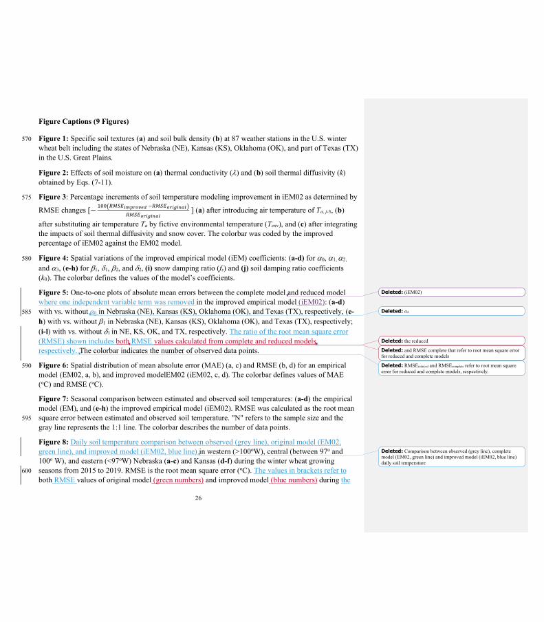
Figure 1: Specific soil textures (a) and soil bulk density (b) at 87 weather stations in the U.S. winter 570 wheat belt including the states of Nebraska (NE), Kansas (KS), Oklahoma (OK), and part of Texas (TX) in the U.S. Great Plains.

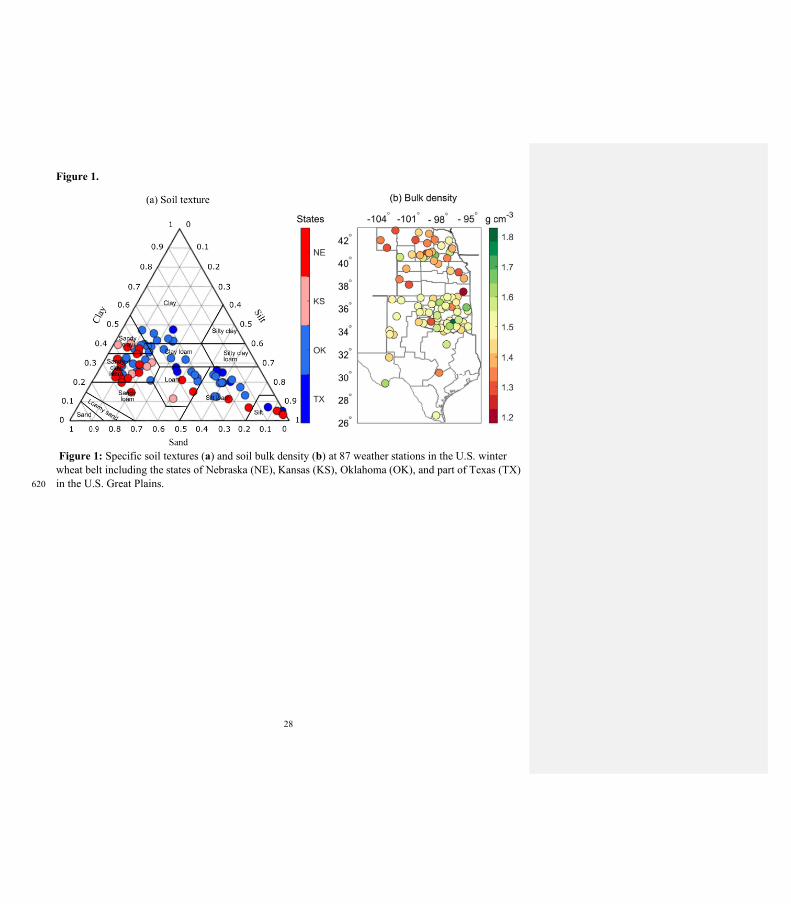
Figure 2: Effects of soil moisture on (a) thermal conductivity (l) and (b) soil thermal diffusivity (k) obtained by Eqs. (7-11).

Figure 3: Percentage increments of soil temperature modeling improvement in iEM02 as determined by 575

RMSE changes [− +));OvD����z����,OvD��z������@OvD��z������

] (a) after introducing air temperature of Ta, j-3, (b)

after substituting air temperature Ta by fictive environmental temperature (Tenv), and (c) after integrating the impacts of soil thermal diffusivity and snow cover. The colorbar was coded by the improved percentage of iEM02 against the EM02 model.

Figure 4: Spatial variations of the improved empirical model (iEM) coefficients: (a-d) for a0, a1, a2, 580 and a3, (e-h) for b1, d1, b2, and d2, (i) snow damping ratio (fs) and (j) soil damping ratio coefficients (k0). The colorbar defines the values of the model’s coefficients.

Figure 5: One-to-one plots of absolute mean errors between the complete model and reduced model where one independent variable term was removed in the improved empirical model (iEM02): (a-d) with vs. without α0 in Nebraska (NE), Kansas (KS), Oklahoma (OK), and Texas (TX), respectively, (e-585 h) with vs. without b1 in Nebraska (NE), Kansas (KS), Oklahoma (OK), and Texas (TX), respectively; (i-l) with vs. without d1 in NE, KS, OK, and TX, respectively. The ratio of the root mean square error (RMSE) shown includes both RMSE values calculated from complete and reduced models, respectively. The colorbar indicates the number of observed data points.

Figure 6: Spatial distribution of mean absolute error (MAE) (a, c) and RMSE (b, d) for an empirical 590 model (EM02, a, b), and improved modelEM02 (iEM02, c, d). The colorbar defines values of MAE (oC) and RMSE (oC).

Figure 7: Seasonal comparison between estimated and observed soil temperatures: (a-d) the empirical model (EM), and (e-h) the improved empirical model (iEM02). RMSE was calculated as the root mean square error between estimated and observed soil temperature. "N" refers to the sample size and the 595 gray line represents the 1:1 line. The colorbar describes the number of data points.

Figure 8: Daily soil temperature comparison between observed (grey line), original model (EM02, green line), and improved model (iEM02, blue line) in western (>100oW), central (between 97o and 100o W), and eastern (<97oW) Nebraska (a-c) and Kansas (d-f) during the winter wheat growing seasons from 2015 to 2019. RMSE is the root mean square error (oC). The values in brackets refer to 600 both RMSE values of original model (green numbers) and improved model (blue numbers) during the

Deleted: (iEM02)

Deleted: α4

Deleted: the reduced

Deleted: and RMSE complete that refer to root mean square error 605 for reduced and complete models

Deleted: RMSEreduced and RMSEcomplete refer to root mean square error for reduced and complete models, respectively.

Deleted: Comparison between observed (grey line), complete model (EM02, green line) and improved model (iEM02, blue line) 610 daily soil temperature

27

periods of October-November, December-January-February, and March-April-May-June, respectively. Shaded areas highlight the winter season (December-February).

Figure 9: The same as Fig. 8 but for western, central, and eastern Oklahoma (a-c) and Texas (d-f).

Deleted: . 615 Deleted: indicate

28

Figure 1.

Figure 1: Specific soil textures (a) and soil bulk density (b) at 87 weather stations in the U.S. winter wheat belt including the states of Nebraska (NE), Kansas (KS), Oklahoma (OK), and part of Texas (TX) in the U.S. Great Plains. 620

29

Figure 2.

Figure 2: Effects of soil moisture on (a) thermal conductivity (l) and (b) soil thermal diffusivity (k) obtained by Eqs. (7-11). 625

30

Figure 3.

Figure 3: Percentage increments of soil temperature modeling improvement in iEM02 as determined by

RMSE changes [− +));OvD����z����,OvD��z������@OvD��z������

] (a) after introducing air temperature of Ta, j-3, (b)

after substituting air temperature Ta by fictive environmental temperature (Tenv), and (c) after integrating 630 the impacts of soil thermal diffusivity and snow cover. The colorbar was coded by the improved percentage of iEM02 against the EM02 model.

31

Figure 4.

Figure 4: Spatial variations of the improved empirical model (iEM) coefficients: (a-d) for a0, a1, a2, 635 and a3, (e-h) for b1, d1, b2, and d2, (i) snow damping ratio (fs) and (j) soil damping ratio coefficients (k0). The colorbar defines the values of the model’s coefficients.

32

Figure 5.

Figure 5: One-to-one plots of absolute mean errors between the complete model and reduced model 640 where one independent variable term was removed in the improved empirical model (iEM02): (a-d) with vs. without α0 in Nebraska (NE), Kansas (KS), Oklahoma (OK), and Texas (TX), respectively, (e-h) with vs. without b1 in Nebraska (NE), Kansas (KS), Oklahoma (OK), and Texas (TX), respectively; (i-l) with vs. without d1 in NE, KS, OK, and TX, respectively. The ratio of the root mean square error (RMSE) shown includes both RMSE values calculated from complete and reduced models, 645 respectively. The colorbar indicates the number of observed data points.

Formatted: Line spacing: Multiple 1.08 li

Deleted: α4

Deleted: the reduced

Deleted: and RMSE

Deleted: 650 Deleted: that refer to root mean square error for reduced and complete models

Deleted: RMSEreduced and RMSEcomplete refer to root mean square error for reduced and complete models, respectively.

Deleted: ¶655

33

Figure 6.

Figure 6: Spatial distribution of mean absolute error (MAE) (a, c) and RMSE (b, d) for an empirical model (EM02, a, b), and improved modelEM02 (iEM02, c, d). The colorbar defines values of MAE (oC) and RMSE (oC).

34

Figure 7. 660

Figure 7: Seasonal comparison between estimated and observed soil temperatures: (a-d) the empirical model (EM), and (e-h) the improved empirical model (iEM02). RMSE was calculated as the root mean square error between estimated and observed soil temperature. "N" refers to the sample size and the gray line represents the 1:1 line. The colorbar describes the number of data points.

35

665

Figure 8.

Figure 8: Daily soil temperature comparison between observed (grey line), original model (EM02, green line), and improved model (iEM02, blue line) in western (>100oW), central (between 97o and 100o W), and eastern (<97oW) Nebraska (a-c) and Kansas (d-f) during the winter wheat growing seasons from 2015 to 2019. RMSE is the root mean square error (oC). The values in brackets refer to 670 both RMSE values of original model (green numbers) and improved model (blue numbers) during the periods of October-November, December-January-February, and March-April-May-June, respectively. Shaded areas highlight the winter season (December-February).

Deleted: <object>Figure 8.¶Figure 8: Comparison between observed (grey line), complete 675 model (EM02, green line) and improved model (iEM02, blue line) daily soil temperature in western (>100oW), central (between 97o and 100o W), and eastern (<97oW) Nebraska (a-c) and Kansas (d-f) during the winter wheat growing seasons from 2015 to 2019. RMSE is the root mean square error (oC). Shaded areas indicate winter 680 season (Dec-Feb).¶

Formatted: Font: Bold

36

Figure 9.

Figure 9: The same as Fig. 8 but for western, central, and eastern Oklahoma (a-c) and Texas (d-f). 685

Formatted: Font: Bold

Deleted: <object>Figure 9. ¶Figure 9: The same as Fig. 9 but for western, central, and eastern Oklahoma (a-c) and Texas (d-

Formatted: Font: Bold