MNRAS 000, 1–21 (2016) Preprint 24 January 2017 Compiled using MNRAS LATEX style file v3.0

H0LiCOW II. Spectroscopic survey and galaxy-groupidentification of the strong gravitational lens systemHE 0435−1223

D. Sluse1?, A. Sonnenfeld2,3,4, N. Rumbaugh5, C. E. Rusu5, C. D. Fassnacht5,T. Treu3, S. H. Suyu6,7,8, K. C. Wong7,9, M. W. Auger10, V. Bonvin11, T. Collett12,F. Courbin11, S. Hilbert13,14, L. V. E. Koopmans15, P. J. Marshall16, G. Meylan11,C. Spiniello6, M. Tewes171 STAR Institute, Quartier Agora - Allee du six Aout, 19c B-4000 Liege, Belgium2 Physics Department, University of California, Santa Barbara, CA, 93106, USA3 Department of Physics and Astronomy, University of California, Los Angeles, CA 90095, USA4 Kavli IPMU (WPI), UTIAS, The University of Tokyo, Kashiwa, Chiba 277-8583, Japan5 Department of Physics, University of California, Davis, CA 95616, USA6 Max Planck Institute for Astrophysics, Karl-Schwarzschild-Strasse 1, D-85740 Garching, Germany7 Institute of Astronomy and Astrophysics, Academia Sinica, P.O. Box 23-141, Taipei 10617, Taiwan8Physik-Department, Technische Universitat Munchen, James-Franck-Straße 1, 85748 Garching, Germany9 National Astronomical Observatory of Japan, 2-21-1 Osawa, Mitaka, Tokyo 181-8588, Japan10 Institute of Astronomy, University of Cambridge, Madingley Road, Cambridge CB3 0HA, UK11 Laboratoire d’Astrophysique, Ecole Polytechnique Federale de Lausanne (EPFL), Observatoire de Sauverny, CH-1290 Versoix, Switzerland12 Institute of Cosmology and Gravitation, University of Portsmouth, Burnaby Rd, Portsmouth PO1 3FX, UK13 Exzellenzcluster Universe, Boltzmannstr. 2, 85748 Garching, Germany14 Ludwig-Maximilians-Universitat, Universitats-Sternwarte, Scheinerstr. 1, 81679 Munchen, Germany15 Kapteyn Astronomical Institute, University of Groningen, PO Box 800, NL-9700 AV Groningen, The Netherlands16 Kavli Institute for Particle Astrophysics and Cosmology, Stanford University, 452 Lomita Mall, Stanford, CA 94035, USA17 Argelander-Institut fur Astronomie, Auf dem Hugel 71, D-53121 Bonn, Germany

Accepted XXX. Received YYY; in original form ZZZ

ABSTRACT

Galaxies located in the environment or on the line of sight towards gravitationallenses can significantly affect lensing observables, and can lead to systematic errorson the measurement of H0 from the time-delay technique. We present the results of asystematic spectroscopic identification of the galaxies in the field of view of the lensedquasar HE 0435−1223 using the W. M. Keck, Gemini and ESO-Very Large telescopes.Our new catalog triples the number of known galaxy redshifts in the direct vicinity ofthe lens, expanding to 102 the number of measured redshifts for galaxies separated byless than 3′ from the lens. We complement our catalog with literature data to gatherredshifts up to 15′ from the lens, and search for galaxy groups or clusters projectedtowards HE 0435−1223. We confirm that the lens is a member of a small group thatincludes at least 12 galaxies, and find 8 other group candidates near the line of sightof the lens. The flexion shift, namely the shift of lensed images produced by highorder perturbation of the lens potential, is calculated for each galaxy/group and usedto identify which objects produce the largest perturbation of the lens potential. Thisanalysis demonstrates that i) at most three of the five brightest galaxies projectedwithin 12′′ of the lens need to be explicitly used in the lens models, and ii) the groupscan be treated in the lens model as an external tidal field (shear) contribution.

Key words: gravitational lensing: strong – quasars: individual: HE 0435−1223–galaxies: groups: general

? dsluse@ulg.ac.bec© 2016 The Authors

2 D. Sluse et al.

1 INTRODUCTION

Ongoing and upcoming cosmological studies deeply rely onthe accurate knowledge of the Hubble constant, H0 (Hu2005; Suyu et al. 2012; Weinberg et al. 2013). The mea-surement of H0 has long been controversial (e.g. Kochanek2002; Kochanek & Schechter 2004), but in the past decadeseveral techniques have measured H0 with a relative uncer-tainty much smaller than 10% (Freedman & Madore 2010;Humphreys et al. 2013; Suyu et al. 2013; Riess et al. 2016).In order to reach the goal of the next decade of cosmologicalexperiments, and be able to e.g. unveil the nature of darkenergy, it is necessary to pin down the accuracy on H0 at thepercent level. This is an ambitious goal and in order to iden-tify unknown systematic errors, it is mandatory to gatherseveral independent constraints on H0 (Weinberg et al. 2013;Riess et al. 2016). The gravitational time-delay technique(Refsdal 1964), applied to a large number of lensed systems,is one of the few techniques allowing one to reach percentprecision on H0 (Suyu et al. 2012). Among the various cos-mological probes, it is also the most sensitive to H0 (e.g.Jackson 2007; Freedman & Madore 2010). By measuring thetime delay ∆t between pairs of lensed images, and model-ing the mass distribution of the lens galaxy, the time delaydistance D∆t can be inferred. As summarized in a recentreview by Treu & Marshall (2016), the technique has longbeen plagued by poor time-delay measurements, invalid as-sumptions about the lens mass profile and systematic errors.However, times have changed. It has been demonstrated thatan exhaustive study of a lensed quasar with high qualitylightcurves (B1608+656; Fassnacht et al. 2002) allows themeasurement of H0 for a single system with a precision of6% (Suyu et al. 2010). In addition, it was shown that thetime-delay technique leads to tight constraints on the othercosmological parameters comparable to those from contem-porary Baryon Acoustic Peak studies, when each probe iscombined with the Cosmic Microwave Background (PlanckCollaboration et al. 2014; Anderson et al. 2014; Planck Col-laboration et al. 2015; Ross et al. 2015).

The improved precision of the time delay techniquestems from the combination of several ingredients. First, theCOSmological MOnitoring of GRAvItational Lenses (COS-MOGRAIL) has been running for over a decade, gatheringexquisite high cadence photometric data for tens of lensedquasars (Eigenbrod et al. 2005; Tewes et al. 2013b). Thoseunprecedented high quality lightcurves combined with newcurve shifting algorithms (Tewes et al. 2013a) now enabletime-delay measurements down to a few percent accuracy(Bonvin et al. 2016; Liao et al. 2016). Second, advancedmodeling techniques that use the full surface brightness ofthe multiple lensed images, containing thousands of pixelsas data points, are now used to constrain the lens mass dis-tribution (Suyu et al. 2009). Third, independent constraintson the lens potential, obtained from the measurement ofthe lens velocity dispersion (Romanowsky & Kochanek 1999;Treu & Koopmans 2002), are now combined with the lensmodels, enabling one to reduce the impact of the mass-sheetdegeneracy1 (Falco et al. 1985; Schneider & Sluse 2013) onthe lens models. Finally, the direct lens environment and

1 The impact on cosmographic inference of other degeneraciesamong lens models, such as the source position transformation

the line-of-sight galaxies are studied in detail (Keeton &Zabludoff 2004; Fassnacht et al. 2006). The observed galaxycounts in the vicinity of the lens are compared to galaxycounts from ray tracing through cosmological simulations toderive a probability distribution of the external convergenceκext produced by over- and under-densities along the line ofsight (Hilbert et al. 2007; Fassnacht et al. 2011).

The H0LiCOW project (H0 Lenses in COSMOGRAIL’sWellspring) aims at achieving better than 3.5% accuracyon H0. To reach this goal, we have gathered a sample offive lenses (B 1608+656, RX J1131−1231, HE 0435−1223,HE 1104−1805, WFI 2033−4723) for which we apply ourmodeling technique on archival and Cycle 20 HST data (PISuyu). The project, together with cosmographic forecastsbased on the full sample, is presented in H0LiCOW Paper I(Suyu et al., submitted). The first two systems have been an-alyzed (Suyu et al. 2010, 2013). To tackle systematic errorsin the other three systems, a stellar velocity dispersion forthe lenses and a study of the lens environments are needed.In this paper, we focus on the spectroscopic identification ofthe brightest galaxies in the field of view of HE 0435−1223,a quadruply imaged quasar at zs = 1.693 ± 0.001 lensedby a foreground elliptical galaxy at zd = 0.4546 ± 0.0002(Wisotzki et al. 2002; Morgan et al. 2005; Sluse et al. 2012b).The main objective of this work is to measure the spectro-scopic redshifts of most of the bright galaxies in the centralregion around HE 0435−1223 (i.e. about 100 galaxies), anecessary observable to measure the contribution of indi-vidual galaxy halos to the surface mass density projectedtowards HE 0435−1223 (Hilbert et al. 2007, 2009; Greeneet al. 2013; Collett et al. 2013). Our secondary objective isto identify major groups and/or galaxy cluster(s), as well asindividual galaxies, at the redshift of the main lens but alsoalong the line of sight, that would perturb non linearly thegravitational potential of the main lensing galaxy. For thatpurpose we complement our data with the spectroscopic cat-alog compiled by Momcheva et al. (2015, hereafter MOM15)that gathers redshifts of ∼ 400 galaxies (about 30 galaxiesare duplicated with our catalog) over a 30′×30′ field cen-tered on HE 0435−1223. The spectroscopic redshift measure-ments are an important ingredient of the statistical analysisof the line of sight towards HE 0435−1223 carried out in thecompanion H0LiCOW Paper III (Rusu et al., submitted).This companion paper presents a weighted count analysisof the galaxies in the field of view of HE 0435−1223 that iscompared to galaxy counts from the Canada-France-Hawaii-Telescope Legacy Survey (CFHTLenS, Heymans et al. 2012)and to galaxy counts from Millennium Simulation (Springelet al. 2005; Hilbert et al. 2007, 2009). This yields a prob-ability distribution of convergence κext produced by theother galaxies in the field. On the other hand, the red-shifts of the galaxies closest in projection to the lens are in-cluded explicitly in the multi-plane lens modeling analysis ofHE 0435−1223 presented in H0LiCOW Paper IV (Wong etal., submitted). Finally, Paper V (Bonvin et al., submitted)presents the time-delay measurements of HE 0435−1223 andthe joint cosmographic inference from the three lensed sys-tems analyzed to-date in H0LiCOW.

(Schneider & Sluse 2014; Unruh et al. 2016), that does not leave

the time-delay ratio invariant, still needs to be quantified.

MNRAS 000, 1–21 (2016)

Environment of HE0435−1223 3

The paper is structured as follows. We present anoverview of the data sets used, of the data reduction pro-cess and redshift measurements in Sect. 2. The methodologyused to identify galaxy groups is explained in Sect. 3. Thegalaxy groups identified with our algorithm and the spectraof the galaxies that are most likely to produce large grav-itational potential perturbations are presented in Sect. 4.Section 5 quantifies the impact of individual galaxies andgalaxy groups on the model. We use the flexion shift toflag the systems that require explicit inclusion in the multi-plane lens models presented in H0LiCOW Paper IV. Fi-nally, Sect. 6 summarizes our main results. In this work,with the exception of the target selection that was based onR−band magnitude in the Vega system, photometric infor-mation comes from the deep multicolor imaging presented inH0LiCOW Paper III and uses the AB photometric system.For convenience, group radii and masses reported in thiswork assume a flat ΛCDM cosmology with cosmological pa-rameters from (Planck Collaboration et al. 2015), namelyH0 = 67.7 km s−1 Mpc−1, Ωm = 0.307. We stress that thischoice has no impact on the group identification as the latterdoes not depend on a specific choice of cosmological param-eters.

2 DATA

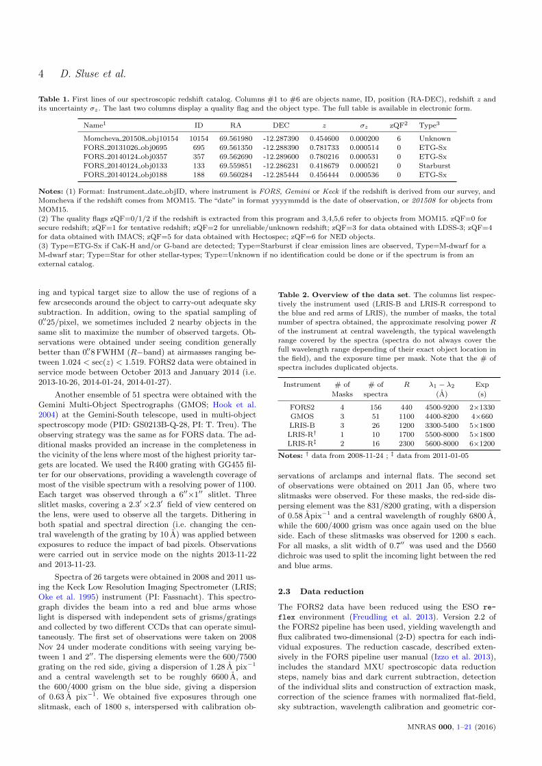
Our data set combines multi-object spectroscopy obtainedat Gemini-South, Keck, and ESO-Paranal observatories. Wedescribe in Sect. 2.1 our target selection methodology. Theobservational setup, and data reduction techniques are de-scribed in Sect. 2.2 & 2.3. Finally, Sect. 2.4 & 2.5 detail howthe spectroscopic redshifts are measured, and evaluate thespectroscopic redshift completeness of our galaxy sample.The catalog and reduced spectra are available in electronicform at the Centre de Donnees astronomiques de Strasbourg(CDS) and from the H0LiCOW website2. The catalog con-tains 534 unique objects, including 368 redshifts exclusivelyreported by MOM15. Our new measurements expands to169 the number of targeted objects separated by less than 3arcmin from the lens. In that range, the new catalog contains103 galaxies (but 16 have only tentative redshifts, and one isthe lens), 42 stars, and 24 objects whose type could not beunambiguously determined and therefore lack redshift. Thefirst five entries of the full catalog are shown in Table 1.

2.1 Target selection

The targets were selected based on a R-band photomet-ric catalog constructed using SExtractor (Bertin & Arnouts1996) applied on archive images obtained with the FOcal Re-ducer and low dispersion Spectrograph for the Very LargeTelescope (FORS1 and FORS2 at VLT). Because of theunavailability of deep frames obtained under photometricconditions, we had to construct an approximate photomet-ric catalog from shallow R-band FORS1 images for which aphotometric zero-point was available, and from deep FORS2z-band frames lacking photometric calibration. By matchingobjects found in both catalogs, hence implicitly assuming a

2 www.h0licow.org/

constant color term, we could get an approximate photom-etry of targets down to R ∼ 23.5 mag. Comparison of thephotometry of the brightest objects in the field with SDSS-DR9 and USNO photometry suggested a photometric ac-curacy of ∼ 0.15 mag. This has been confirmed a-posterioriusing the deep Subaru/Suprime-Cam r−band photometrypresented in H0LiCOW Paper III. The photometry of thetwo catalogs agree with each other with a scatter on thedifference of 0.17 mag. In the analysis presented here we donot use that preliminary photometry but the most accurateone presented in H0LiCOW Paper III. Keeping in mind theimportance of identifying all the faint galaxies in the closevicinity of the lens, we have prioritized the spectroscopictargets using the following scheme. Any potential galaxy(i.e. objects with SExtractor flag CLASS_STAR < 0.98) withR < 23.5 mag located within a 30′′ radius from the main lenswas given highest priority (i.e. P1). Any potential galaxywith R < 21 mag located within 3′ from the lens was alsoflagged as high priority (P1). This selection towards brightobjects was set to avoid missing the identification of of mas-sive nearby galaxy clusters. Medium priority (P2) objectswere galaxies with 21 < R < 22.4 mag located in an annu-lus 0′.5 < r < 1′ from the lens. Finally, lower priority objects(P3) were those galaxies beyond 1′ from the lens (but within3′), with 21 < R < 22 mag. Any object not entering in theabove categories was used as a filler and targeted if free slitswere available. When possible, we tried to observe again thefaintest targets (i.e. R < 22.4 mag) to increase the signal-to-noise ratio in their spectra. We have compared, a posteriori,our original object selection with the one we would have car-ried out based on the deeper Subaru/Suprime-Cam photom-etry (which has a magnitude limit of r = 25.94± 0.28 mag).We found that 1 (P1), 3 (P2) and 4 (P3) objects were missedin the original catalog. This corresponds to typically 10%of missed targets. Those mismatches were caused by differ-ences in SeXtractor parameters yielding inaccurate deblend-ing rather than by the photometric inaccuracy of the originalcatalog. The impact of spectroscopic incompleteness on ouranalysis is discussed in Sect. 2.5 & 4. Figure 1 shows thefield around HE 0435−1223 targeted by our program. Tar-gets with secured redshifts, tentative redshifts, failed redshiftmeasurements, and unobserved galaxies, are respectively de-picted with colored circles, colored boxes, black boxes andgray circles.

2.2 Observations

The largest data set has been obtained with the FORS2instrument (Appenzeller et al. 1998) mounted at theCassegrain focus of the UT1 (Antu) telescope (PID: 091.A-0642(A), PI: D. Sluse). The instrument was used in its multi-object spectroscopy mode with exchangeable masks (MXU),where masks are laser cut at the location of the targets. TheGRIS300V grism + GG435 blocking filter were used to en-sure a large spectral coverage (see Table 2) in order to maxi-mize the range of redshift detectability. Four masks with dif-ferent orientations on the sky were employed to best coverthe 6′× 6′ field of view centered on HE 0435−1223. Eachmask was composed of approximately 40 slits of 1′′ widthand typically 8 ′′ long (the slit length was reduced by a fewarcseconds for some objects to avoid overlap of spectra).This slit length was sufficiently large compared to the see-

MNRAS 000, 1–21 (2016)

4 D. Sluse et al.

Table 1. First lines of our spectroscopic redshift catalog. Columns #1 to #6 are objects name, ID, position (RA-DEC), redshift z and

its uncertainty σz . The last two columns display a quality flag and the object type. The full table is available in electronic form.

Name1 ID RA DEC z σz zQF2 Type3

Momcheva 201508 obj10154 10154 69.561980 -12.287390 0.454600 0.000200 6 UnknownFORS 20131026 obj0695 695 69.561350 -12.288390 0.781733 0.000514 0 ETG-Sx

FORS 20140124 obj0357 357 69.562690 -12.289600 0.780216 0.000531 0 ETG-Sx

FORS 20140124 obj0133 133 69.559851 -12.286231 0.418679 0.000521 0 StarburstFORS 20140124 obj0188 188 69.560284 -12.285444 0.456444 0.000536 0 ETG-Sx

Notes: (1) Format: Instrument date objID, where instrument is FORS, Gemini or Keck if the redshift is derived from our survey, and

Momcheva if the redshift comes from MOM15. The “date” in format yyyymmdd is the date of observation, or 201508 for objects from

MOM15.(2) The quality flags zQF=0/1/2 if the redshift is extracted from this program and 3,4,5,6 refer to objects from MOM15. zQF=0 for

secure redshift; zQF=1 for tentative redshift; zQF=2 for unreliable/unknown redshift; zQF=3 for data obtained with LDSS-3; zQF=4

for data obtained with IMACS; zQF=5 for data obtained with Hectospec; zQF=6 for NED objects.(3) Type=ETG-Sx if CaK-H and/or G-band are detected; Type=Starburst if clear emission lines are observed, Type=M-dwarf for a

M-dwarf star; Type=Star for other stellar-types; Type=Unknown if no identification could be done or if the spectrum is from an

external catalog.

ing and typical target size to allow the use of regions of afew arcseconds around the object to carry-out adequate skysubtraction. In addition, owing to the spatial sampling of0.′′25/pixel, we sometimes included 2 nearby objects in thesame slit to maximize the number of observed targets. Ob-servations were obtained under seeing condition generallybetter than 0.′′8 FWHM (R−band) at airmasses ranging be-tween 1.024 < sec(z) < 1.519. FORS2 data were obtained inservice mode between October 2013 and January 2014 (i.e.2013-10-26, 2014-01-24, 2014-01-27).

Another ensemble of 51 spectra were obtained with theGemini Multi-Object Spectrographs (GMOS; Hook et al.2004) at the Gemini-South telescope, used in multi-objectspectroscopy mode (PID: GS0213B-Q-28, PI: T. Treu). Theobserving strategy was the same as for FORS data. The ad-ditional masks provided an increase in the completeness inthe vicinity of the lens where most of the highest priority tar-gets are located. We used the R400 grating with GG455 fil-ter for our observations, providing a wavelength coverage ofmost of the visible spectrum with a resolving power of 1100.Each target was observed through a 6′′×1′′ slitlet. Threeslitlet masks, covering a 2.3′×2.3′ field of view centered onthe lens, were used to observe all the targets. Dithering inboth spatial and spectral direction (i.e. changing the cen-tral wavelength of the grating by 10 A) was applied betweenexposures to reduce the impact of bad pixels. Observationswere carried out in service mode on the nights 2013-11-22and 2013-11-23.

Spectra of 26 targets were obtained in 2008 and 2011 us-ing the Keck Low Resolution Imaging Spectrometer (LRIS;Oke et al. 1995) instrument (PI: Fassnacht). This spectro-graph divides the beam into a red and blue arms whoselight is dispersed with independent sets of grisms/gratingsand collected by two different CCDs that can operate simul-taneously. The first set of observations were taken on 2008Nov 24 under moderate conditions with seeing varying be-tween 1 and 2′′. The dispersing elements were the 600/7500grating on the red side, giving a dispersion of 1.28 A pix−1

and a central wavelength set to be roughly 6600 A, andthe 600/4000 grism on the blue side, giving a dispersionof 0.63 A pix−1. We obtained five exposures through oneslitmask, each of 1800 s, interspersed with calibration ob-

Table 2. Overview of the data set. The columns list respec-

tively the instrument used (LRIS-B and LRIS-R correspond tothe blue and red arms of LRIS), the number of masks, the total

number of spectra obtained, the approximate resolving power Rof the instrument at central wavelength, the typical wavelength

range covered by the spectra (spectra do not always cover the

full wavelength range depending of their exact object location inthe field), and the exposure time per mask. Note that the # of

spectra includes duplicated objects.

Instrument # of # of R λ1 − λ2 Exp

Masks spectra (A) (s)

FORS2 4 156 440 4500-9200 2×1330

GMOS 3 51 1100 4400-8200 4×660LRIS-B 3 26 1200 3300-5400 5×1800

LRIS-R† 1 10 1700 5500-8000 5×1800

LRIS-R‡ 2 16 2300 5600-8000 6×1200

Notes: † data from 2008-11-24 ; ‡ data from 2011-01-05

servations of arclamps and internal flats. The second setof observations were obtained on 2011 Jan 05, where twoslitmasks were observed. For these masks, the red-side dis-persing element was the 831/8200 grating, with a dispersionof 0.58 Apix−1 and a central wavelength of roughly 6800 A,while the 600/4000 grism was once again used on the blueside. Each of these slitmasks was observed for 1200 s each.For all masks, a slit width of 0.7′′ was used and the D560dichroic was used to split the incoming light between the redand blue arms.

2.3 Data reduction

The FORS2 data have been reduced using the ESO re-

flex environment (Freudling et al. 2013). Version 2.2 ofthe FORS2 pipeline has been used, yielding wavelength andflux calibrated two-dimensional (2-D) spectra for each indi-vidual exposures. The reduction cascade, described exten-sively in the FORS pipeline user manual (Izzo et al. 2013),includes the standard MXU spectroscopic data reductionsteps, namely bias and dark current subtraction, detectionof the individual slits and construction of extraction mask,correction of the science frames with normalized flat-field,sky subtraction, wavelength calibration and geometric cor-

MNRAS 000, 1–21 (2016)

Environment of HE0435−1223 5

rection. Default parameters of reduction routines were used,except for the wavelength calibration where a polynomialof degree n = 4 gave the best solution with residuals dis-tributed around 0, a RMS of typically 0.1-0.2 pixels at allwavelengths and a model accuracy derived by matching thewavelength solution to the sky lines, to 0.2 A. Cosmic rayshave not been removed within the pipeline but separately,using the LA-COSMIC routine (van Dokkum 2001). Extrac-tion was subsequently performed using customized Pythonroutine fitting 1-D Gaussian profile on each wavelength binof the rectified 2-D spectrum. When multiple objects werepresent in the same slit, a sum of profiles centered on eachtarget was used for the extraction. For each mask, a set oftwo exposures were obtained. The one-dimensional spectraextracted on individual exposures were finally co-added.

GMOS data were reduced using the Gemini IRAF3

package. Dedicated routines from the gemini-gmos sub-package were used to perform bias subtraction, flat-fielding,slit identification, geometric correction, wavelength calibra-tion and sky subtraction on each exposure, producing awavelength calibrated 2-D spectrum for each slitlet. Wave-length calibration was done in interactive mode: we visu-ally inspected the automatic identification of arc lamp linesproduced by the pipeline and applied corrections in casesof mis-identification. We then used a custom Python scriptto extract one dimensional (1-D) spectra for each detectedobject in each slitlet and to co-add spectra from differentexposures of the same mask.

The Keck/LRIS data were reduced with a customPython package that has been developed by our team. Thispackage automatically performs the standard steps in spec-troscopic data calibration including overscan subtraction,flat-field correction, rectification of the two-dimensionalspectra, and wavelength calibration. For the red-side spec-tra, the wavelength calibration was derived from the numer-ous night sky-lines in the spectra, while on the blue sidethe arclamp exposures were also used. The 1-D spectra wereextracted from each exposure through a given slitmask us-ing gaussian-weighted profiles. The extracted spectra wereco-added using inverse-variance weighting.

2.4 Redshift measurement

The redshift measurements of the FORS2 (151 objects),GMOS (51 objects), and LRIS (26 objects) data were per-formed by cross-correlating the 1-D spectra with a set ofgalactic (Elliptical, Sb, only galactic emission lines, quasar)and stellar (G, O, M1, M8, A spectral types, all-stars) tem-plates using the xcsao task, part of the rvsao IRAF package(version 2.8.0). The package was used in interactive mode,excluding regions where the sky subtraction was not optimal.The redshift measurement was then flagged as secure (70%of the measurements), tentative (15% of the measurements)or unsecure (15% of the measurements) based on the qualityof the cross-correlation, signal-to-noise and number of emis-sion/absorption lines detected. The formal uncertainty on

3 IRAF is distributed by the National Optical Astronomy Obser-

vatories, which are operated by the Association of Universities forResearch in Astronomy, Inc., under cooperative agreement with

the National Science Foundation.

the redshift from this procedure depends only on the widthand peak of the cross-correlation. This formal uncertainty issmaller than the systematic error on the wavelength calibra-tion. The latter has been derived by comparing redshifts ofobjects in common with the catalog4 published by MOM15(see Appendix A and Fig. A1). The 30 galaxies in commonwith that catalog5 reveal a systematic offset δz ∼ -0.0004between the two samples, or ∼ 1 pixel ∼ 3.3 A in our wave-length calibration (i.e. about five times larger than the onederived along the reduction). This translates into a velocityoffset δv ∼ 120 km s−1. We account for this error in the fol-lowing way. On one side, we subtract δz ∼ 0.0004 from theFORS redshifts, and on the other hand, we add quadrati-cally an error σz = 0.0005 to the formal redshift error. Thisuncertainty has a negligible impact on our group detectionscompared to other sources of errors (see Sect. 4.2).

The comparison between multiple data sets also pro-vides a good way to flag incorrect redshift measurements.Table 3 lists the three objects that have been reported inMOM15 with a redshift significantly different from ours.Two of the redshift estimates from MOM15 are tentativeliterature measurements from Morgan et al. (2005). The red-shift of these galaxies, labeled G09 and G10 in Morgan et al.(2005), was then based on a possible detection of [O II] line.Our spectra, as well as HST images, show that these ob-jects are stars in our Galaxy. The third object (ID 11182 inMOM15) has a complex morphology and could potentiallybe a blend of two objects. We clearly detect Hβ, Hα, and[O III]λλ4959, 5007 emission at a redshift z = 0.1537. Theredshift z = 0.5484 proposed by MOM15 roughly matchesa mis-identification of [O III] λ 5007 as [O II]λ 3727 emission,which would explain the observed discrepancy. No groupsare detected at the redshifts of those misidentified objects(Sect. 4.2).

2.5 Completeness of the spectroscopic redshifts

For the analysis presented in this paper, we have comple-mented our data with the spectroscopic catalog of MOM15(343 new galaxies separated by up to 15′ from the lens), andwith i−band magnitudes (i.e. i′ filter from Subaru/Suprime-Cam, similar to SDSS-i filter) from H0LiCOW Paper III.

We evaluate the spectroscopic redshift completeness asa function of various criteria by comparing our spectroscopicand photometric catalogs. Figure 2 shows, as a function ofi−band magnitude, the number of galaxies (total, and withsecure spectroscopic redshift, hereafter spec-z ) in the field ofthe lens. The number of galaxies with a secure spec-z dropssignificantly above i = 22.5 mag, as expected from our obser-vational setup. Another important piece of information forour analysis is the completeness of our sample as a functionof the magnitude of the galaxies and of the distance to thelens. Figure 3 shows that our completeness is higher than60% in the inner 2′ around the lens for galaxies brighter

4 Only 8 galaxies have redshift measurements from both Gemini

and FORS, and a handful from Keck and FORS, which limits ourability to perform internal comparisons.5 We only consider objects with the same redshift and with flags3 and 4, i.e. we exclude objects that are not new measurements

from MOM15 but included in their catalog.

MNRAS 000, 1–21 (2016)

6 D. Sluse et al.

4h38m05s10s15s20s25s

RA (J2000)

20′00′′

19′00′′

18′00′′

17′00′′

16′00′′

−1215′00′′

Dec

(J20

00)

0.0

0.1

0.2

0.3

0.4

0.5

0.6

0.7

0.8

z

star

HE0435

G2

G1

G5

G3

G45”

No spectra

→ zQF=0 (galax)

? Stars w. spectra2 zQF=2 / no spec-z→22 zQF=1 (galax)

Figure 1. Overview of the spectroscopic redshift obtained from our new and literature data in a field of view of ∼ 3′×3′ aroundHE 0435−1223 (black box and inset panel). Spectroscopically identified stars are marked with a red ”Star” symbol, while galaxies are

marked with a circle whose size scales with its i-band magnitude (largest colored circle correspond to i ∼17 mag, smallest to i ∼23 mag),

and color indicates the redshift (right color bar). A gray circle is used when no spectroscopic data are available. Galaxies that have beentargeted but for which no spec-z could be retrieved are shown as open black squares, those with a tentative redshift (zQF = 1, see Table 1)with a colored square. The background frame shows the central region of deep 600 s i−band image obtained with Subaru/Suprime-Cam

and presented in H0LiCOW Paper III.

Table 3. Objects with significantly different redshifts in MOM15 and in our catalog. The last comment briefly summarizes the reason

of the likely mis-identification in MOM15 (see Sect. 2.4 for more details).

(RA,DEC) ID-MOM ID zMOM (σz) z (σz) Note

(69.57627, -12.28224) 10541 251 0.3380 (2.0E-4) 0. (0.001) Based on spurious [O II].

(69.57391, -12.27961) 10425 249 0.3691 (2.0E-4) 0. (0.001) Based on spurious [O II].(69.58917, -12.29916) 11182 95 0.54839 (2.3E-4) 0.15307 (9.3E-5) Mis-identified [O II] or blend of 2 objects.

than i ∼ 22 mag. At larger distances, or fainter magnitudecutoff, the completeness of the spectroscopic catalog dropsbelow 30%.

Identifying galaxy groups requires a high spectroscopiccompleteness over the chosen field of view. Based on Fig-

ure 3, we have decided to limit our search for groups to amaximum distance of r ∼ 6′ of the lens. With this radius,we cover a region ∼ 3 virial radius Rvir of a typical groupat z = 0.4 ± 0.2 (i.e. Rvir ∼ 1 Mpc or θvir ∼ 2′), and arecomplete at more than 50% down to i = 22 mag. We show

MNRAS 000, 1–21 (2016)

Environment of HE0435−1223 7

16 17 18 19 20 21 22 23 24

i (mag)

0.0

0.5

1.0

1.5

2.0

2.5

3.0

log(N

)

photometricspectroscopic

Figure 2. Apparent i−band magnitude histogram (log scale) ofall the galaxies (thin blue) located within 6′ of HE 0435−1223

and of the subsample of galaxies with a spectroscopic redshift(thick red).

18 19 20 21 22 23 24

i (mag)

0.0

0.2

0.4

0.6

0.8

1.0

Frac

tion

ofsp

ec-z

rmax=2.0’rmax=6.0’rmax=10.0’

0 2 4 6 8 10 12 14

Distance (’)

0.0

0.2

0.4

0.6

0.8

1.0imax=21.0magimax=22.0magimax=23.0mag

Figure 3. Left: Fraction of spectroscopic redshifts (unsecure

redshifts are not included) as a function of the maximum i-band magnitude of the sample, for three different radii 2′(solid-

blue), 6′(dashed-red), 10′ (dashed-dotted-green). Right: Fractionof spectroscopic redshifts as a function the maximum distance to

the lens for three different limiting magnitude (imax = 21 mag

in solid-blue; imax = 22 mag in dashed-red, imax = 23 mag indotted-dashed-green). The error bars are the Poisson noise de-

rived from the number of objects studied.

in Sect. 5 that this is sufficient to identify groups that pro-duce high order perturbations of the gravitational potentialof HE 0435−1223.

We have also derived the fraction of objects with spec-z as a function of galaxy stellar mass. For that purpose,we use the mass and photometric redshifts (hereafter photo-z ) estimates obtained in H0LiCOW Paper III from multi-color optical photometry6. The left panel of Figure 4 showsthat our spectroscopic sample is not mass-biased down toi ∼ 22 mag. For a limiting magnitude i ∼ 23 mag, the pho-

6 Stellar masses derived using optical (ugri) + near infrared(JHKs) photometry were calculated only for the inner 2′ around

the lens due to the smaller field of view covered by the near in-frared images. Consequently, we have only used stellar massesbased on ugri photometry.

7 8 9 10 11 12log(M∗/M¯)

0

50

100

150

200

250

300

350

400

450

N

imax (mag)

phot-z212223

spec-z212223

7 8 9 10 11 12log(M∗/M¯)

0.0

0.2

0.4

0.6

0.8

1.0

Fract

ion o

f sp

ec-

z

imax (mag)

21.022.023.0

Figure 4. Characteristics of the spectroscopic sample for galax-

ies located at less than 6′ from HE 0435−1223. Left: Number

of galaxies as a function of the stellar mass for the photomet-ric (solid) and spectroscopic (dashed) samples for three different

cuts in magnitudes imax = (21, 22, 23) mag (in resp. blue, red,

green). To ease legibility, for each magnitude cut, the peak ofthe distribution of the spectroscopically confirmed galaxies has

been normalized by a factor n = (1.6, 2.5, 4.8) to match the cor-responding peak (i.e. imax = (21, 22, 23) mag) of the photometric

sample. Right: Fraction of spectroscopic redshifts as a function

of the stellar mass for three different limiting magnitude imax =(21, 22, 23) mag.

tometric and spectroscopic distributions start to differ moresignificantly. This is because most of our spectroscopicallyconfirmed galaxies have magnitudes i < 22 mag (Fig. 2).The right panel of Figure 4 shows that the completeness ofthe spectroscopic sample is the highest (40-50%) at the highmass end (i.e. M∗ ∼ 1012 M), even down to i = 23 mag,and remains above 30% down to typically M ∼ 1010M.

3 GALAXY GROUP IDENTIFICATION

Our main objective is the identification of groups locatedclose in projection to HE 0435−1223 as they are the mostlikely to influence the time delay between the lensed images.This requires a method sensitive enough to allow the de-tection of low mass and compact groups but also of loosegroups. Spectroscopy-based techniques are particularly wellsuited for this aim but demand adaptive selection crite-ria. In general, group candidates are first identified basedon peaks in redshift space, and then group membership isrefined based on the spatial proximity between candidategroup galaxies. The latter is assessed either based on the as-pect ratio between the velocity-space group elongation alongthe line of sight (the “finger of God effect”) and its trans-verse extension (e.g. Wilman et al. 2005; Munoz et al. 2013),or on a proxy for the group virial radius (e.g. Calvi et al.2011; Ammons et al. 2014). After experimentation, we foundthat the use of the aspect ratio to assess group membershipyields detection of a larger number of groups than usingRvir, additional groups being often poor groups and pos-sibly yet non virialized structures. We therefore used thatselection criterion because it provides a more complete cen-sus of groups and allows us to conservatively estimate theirimpact on the gravitational lensing potential. For the sakeof completeness, we report and discuss the results obtainedwith the virial radius criterion in Appendix B. The generaldesign of our algorithm is described below.

MNRAS 000, 1–21 (2016)

8 D. Sluse et al.

3.1 Group identification

Our strategy to identify galaxy groups consists of two mainsteps. The first step is building a trial group catalog. Fol-lowing Ammons et al. (2014), we identify group candidatessimply based on peaks in redshift space. Potential groupredshifts are detected by selecting peaks of at least 5 mem-bers in redshift space with redshifts grouped in bins of 2000km s−1(observed frame). Groups of less than 5 members areunlikely to play an important role in the lens analysis asthey most likely have a low velocity dispersion (i.e. σ peaksat ∼100 km s−1, Robotham et al. 2011). The operation is re-peated after shifting the bin centers by half the bin-width toavoid missing a peak due to an inadequate binning. Then,the potential group members are selected as being galax-ies located within ±1500 km s−1of the peak, correspondingroughly to three times the velocity dispersion of a groupwith Mvir ∼ 1013.7 − 1014 M. Additional neighbor galaxiesin redshift space are included in the group if they are locatedless than 1500 km s−1from another candidate group member.A trial group catalog can then be constructed. These conser-vative starting criteria are meant to enhance our sensitivityto small groups, which typically will have velocity disper-sions of a few hundred km s−1. A bi-weight estimator (Beerset al. 1990) is used to calculate the mean redshift and veloc-ity dispersion of the group candidates. The groups centroidis determined as a luminosity weighted centroid (Wilmanet al. 2005; Robotham et al. 2011).

The trial groups obtained are the starting point for thesecond step of our algorithm that measures the spatial sep-aration between galaxies sharing similar redshifts, and iter-atively refine the group properties. The procedure removesthose galaxies that are too far in the outskirts of the groupand/or in the tail of the group redshift distribution. Thealgorithm follows a methodology similar to that of Wilmanet al. (2005) as described below.

(i) The initial group redshift is derived from our trialgroup catalog. Because the selection criterion of the trial cat-alog is very conservative it largely overestimates the groupvelocity dispersion. In order to identify even small groups, weproceed like Wilman et al. (2005) and initially set σobs = 500km s−1. That value is revised in subsequent iterations of thealgorithm.

(ii) Galaxies that are more than n times the group ve-locity dispersion from the group redshift are excluded. Thiscorresponds to the following limit in redshift space:

δzmax = n× σobs/c, (1)

where n = 2 is used, and σobs is the group velocity dispersionuncorrected for redshift measurement errors.

(iii) The maximum angular transverse extension of thegroup δθmax is derived assuming an aspect ratio b = 3.5 forthe group, giving

δθmax = 206265′′c× δzmax

(b (1 + z)H(z)Dθ(z))(2)

where Dθ(z) is the angular diameter distance to redshift z.(iv) The angular separation between each galaxy and the

i-band luminosity weighted group centroid is derived andgalaxies that have δθ < δθmax and |z − zgroup| < δzmax arekept as group members. If a galaxy lacks a reliable pho-tometric measurement (this happens for about 5% of the

galaxies of our catalog), we do not use a luminosity weight-ing scheme for the galaxy centroid. This has no impact onthe group detection but generally changes appreciably thegroup centroid. The difference in group centroid position hasno significant impact on the cosmological analysis performedin H0LiCOW Paper V.

(v) The observed group velocity dispersion σobs is recal-culated using the gapper algorithm (Beers et al. 1990) if thegroup contains fewer than 10 galaxies, and a bi-weighted es-timator otherwise. This procedure is known to provide a lessbiased estimate of the velocity dispersion (Beers et al. 1990;Munoz et al. 2013). If during this iterative process the num-ber of group members falls below 4, the standard deviationis used instead, as none of the other technique provides re-liable estimate of σobs for a small number of objects. At thesame time we also derive an improved group redshift usingthe bi-weight estimator, or the mean when we are left withfewer than 4 members.

(vi) A new centroid is redefined based on the new mem-bers, and a new group redshift zgroup is derived using a bi-weight estimator. The whole process (from ii) is repeateduntil a stable solution is reached. A solution is generallyfound after three to five iterations.

Once a stable solution is reached, the intrinsic veloc-ity dispersion of the group (i.e. obtained after convert-ing galaxy velocities to rest frame velocities using vrest =c (z− zgroup)/(1+ zgroup)) is computed, removing in quadra-ture the average measurement error of the group galaxiesfrom the (rest-frame) velocity dispersion (Wilman et al.2005).

3.2 Caveats

The group detection depends to some extent on the choiceof the parameters used in our iterative algorithm, in partic-ular of the value of the aspect ratio b and of the rejectionthreshold in velocity space (i.e. n in Eq. (1)). The fiducialvalues used for those parameters have been chosen based onthose used in Wilman et al. (2005). We experimented withdifferent choices, including aspect ratio b = 11 (as found insome numerical simulations, e.g. Eke et al. 2004), rejectionthreshold n = 3. We found that the fiducial value of b tendsto maximize the number of group members as well as thechance of detection of a group at a given peak in redshiftspace. The choice of rejection threshold at n = 3 favors theidentification of larger groups with multiple peaks in redshiftspace, suggesting that non-group members are included.

4 ENVIRONMENT AND LINE OF SIGHTCHARACTERISTICS

Individual galaxies located close in projection to the mainlens, as well as more distant galaxy groups, can significantlymodify the structure of the lensing potential. In such a case,they need to be included explicitly in the lens model (Mc-Cully et al. 2016). We show in Sect. 4.1 the spectra of thefive galaxies that yield the most important perturbations ofthe lens potential. In Sect. 4.2 & 4.3, we present and dis-cuss the results of our search for important groups in thefield of view of the lens. These results will be used in Sect. 5

MNRAS 000, 1–21 (2016)

Environment of HE0435−1223 9

where we quantify the amplitude of the perturbation causedby these structures.

4.1 Nearby galaxies

When we initiated our spectroscopic follow-up, we were lack-ing color information for the galaxies in the field, precludingany selection based on photometric redshift or stellar mass.We therefore prioritized the follow-up based on the lumi-nosity and projected distance to the lens (Sect. 2.1). Fivebright galaxies (i < 22.5 mag) are detected at a projecteddistance of r < 15′′ from the lens (Figure 1). Those galaxies,G1 to G5, were labeled G22, G24, G12, G21, G23 in Mor-gan et al. (2005). Following the methodology proposed byMcCully et al. (2016) and presented in Sect. 5, we have ver-ified a posteriori (using photo-z and stellar mass, for galaxieswithout spec-z), that those galaxies are the most likely toinfluence substantially the modeling, the other faint galaxiesdetectable in the vicinity of the lens not yielding significantperturbation of the lens potential. Figure 5 show the spectraand measured redshifts of galaxies G1 to G5. Three of themare first time measurements. Chen et al. (2014) previouslyreported a redshift z = 0.4188 for G3 (as well as Morganet al. 2005), and z = 0.7818 for G1. Those measurementsare statistically compatible with ours.

The most important perturber (see Sect. 5), the galaxyG1, lies in the background of the lens at z ∼ 0.78. It ispotentially part of a small galaxy group of up to 4 spec-troscopically identified members, including the two nearbygalaxies G2 and G5. The galaxy G4 located ∼ 9′′ N-W ofthe lensing galaxy, is in the direct environment of the lens,and part of a larger group of galaxies at the lens redshift(see Sect. 4.2). The galaxy G3, at z ∼ 0.419, and located atδθ ∼ 8.′′6 W-N-W from HE 0435−1223, is the second mostimportant source of perturbation of the gravitational po-tential after G1 (Sect. 5). The lens models presented inH0LiCOW Paper IV systematically include G1 using multi-lens plane formalism, while G2 to G5, which are found toimpact less significantly the lens models due to their largerprojected distance to the lens (see Sect. 5), are included inone of the systematic tests presented in that paper.

4.2 Groups: overview

Important perturbations to the lens potential are not onlycaused by individual galaxies, but can also be produced bymore distant and massive groups along the line of sight, orby a group at the lens redshift. In order to flag those po-tential perturbers, it is mandatory to be able to detect evenlow-mass groups along line of sight that have their centroidlocated in projection within a few arcminutes from the lens,namely the virial radius of a typical group at the lens red-shift. Owing to the spectroscopic completeness of our sam-ple, we first apply our group finding algorithm (Sect. 3.1) toa region of 6′ radius around the lens, where we have spec-troscopically identified 1/3 of the galaxies down to i = 22mag. Out of the ten peaks in redshift space observed in thatrange (Fig. 6), seven lead to a group identification with ouriterative procedure (Table 4).

By limiting the group search to a small field, we mayunderestimate the group richness, and in particular miss an

important fraction of the galaxies lying in rich groups witha projected center significantly offset with respect to thelens position on the sky. It is therefore necessary to expandour search up to the largest radius available, namely 15′, inorder to identify those structures. At those radii, the spec-troscopic completeness drops significantly, but this is com-pensated by our quest for only the richest groups7. In addi-tion, because the group properties are particularly uncertainwhen the number of galaxy members is small and spectro-scopic incompleteness high, we search for groups within 15′

of the lens only around peaks in redshift space of at least10 galaxies. This choice is guided by the results obtained atsmaller radii where group properties are more robustly re-trieved above 10 galaxies. It is also above this threshold thatour estimator of the group velocity dispersion is expected tobe the most accurate (Beers et al. 1990). From the ten peaksfound in redshift space (Fig. 6), only six are found to be as-sociated with groups of at least five members (Table 4). Twoof these groups were undetected when we limited our searchto a maximum separation of 6′ from the lens.

A complementary approach would be to search forgroups based on photometric redshifts. Although, this tech-nique should allow the detection of overdensities of galax-ies with reasonable efficiency (Williams et al. 2006; Gillis& Hudson 2011), it would not allow us to characterize thegroup properties with sufficient accuracy due to the too largeuncertainty on individual photometric redshifts (σz = 0.07),and of a small bias at the level σsys

z = 0.007.In total, we have identified 9 groups. Their properties

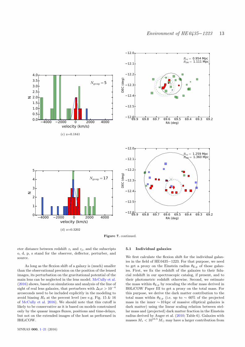
are listed in Table 4, their spatial and redshift distributionare shown in Fig. 7, and an estimate of their virial mass andradius is provided in Appendix C. The redshift distributionand spatial extension of two groups, at z = 0.5059 and z =0.5650, suggest that these groups could be bimodal (Fig. 7),namely constituted of two or more subgroups not identifiedas seperated structures by our algorithm. The use of thevirial radius to identify groups (Appendix B) yields groupdetection at the same redshifts but for two groups (z =0.4185 and z = 0.7019). The group properties are compatiblebetween the two selection criteria for all commonly identifiedgroups except the possibly bimodal groups, and the groupat z ∼ 0.32. These differences are discussed in Appendix B.We also note that not using luminosity weighting centroidyields detection of two more group candidates: a group atz=0.3976 (σint = 143±51 km s−1, FOV=6′), and a group atz = 0.5651 (σint = 259± 75 km s−1, N = 5, FOV=15′).

Error bars on the velocity dispersion and centroid havebeen derived using a bootstrapping approach. This consistsin constructing 1000 samples of each group, each sample hav-ing the same richness as the fiducial group, but with mem-bers randomly chosen among the fiducial ones (repetitionsbeing allowed). When constructing the samples, we have in-dependently bootstrapped the positions, redshifts and lumi-nosity of the galaxies, and derived the group properties inthe same way as for the real group (but we did not apply our

7 Note that small groups at low redshifts can potentially havetheir centroid close in projection to the lens while being detectable

only based on large area search due to their higher angular virialradius. However, the redshift difference between those groups and

the main lens ensures a small effective impact on the lens poten-

tial, see Sect. 5

MNRAS 000, 1–21 (2016)

10 D. Sluse et al.

0.000.200.400.600.80

0.000.010.020.040.05

0.000.040.070.110.14

0.000.020.040.050.07

3500 4000 4500 5000

Rest-frame wavelength (Å)

0.000.010.010.010.02

G1: z=0.78213

G2: z=0.78062

G3: z=0.41908

G4: z=0.45684

G5: z=0.77919

Flux (

arb

itra

ry u

nit

s)

Figure 5. Rest-frame spectra of the galaxies G1-G5 (blue; see Fig. 1 for identification) over-plotted with the best galaxy template (red)used to measure the redshift with the cross-correlation technique. For legibility, the spectra have been smoothed with a 5 pixels boxcar,

and the templates have been multiplied by a third order polynomial to correct for uncertainties in the instrumental response. Gray bands

indicate regions affected by sky subtraction problems.

0.0 0.2 0.4 0.6 0.8 1.0

redshift

0

5

10

15

20

25

N

Radius (arcmin)

156

Figure 6. Redshift distribution of the objects within aperturesof 6′(red) and 15′(black) centered on the lens. The redshifts of

the groups identified with our algorithm (Tab. 4) are shown asvertical dashed lines. Note that the height of the peaks changes

when the bin center is offset by half the bin width. This “redshift-phase” effect is accounted for in our group detection algorithm(Sect. 3.1).

iterative algorithm on the sample). The final uncertainty onthe scrutinized group property is the standard deviation ofthe bootstrap distribution.

4.3 Groups: discussion

For consistency, we can compare the number of groups wefound with the average density of groups found in large sur-veys. A good comparison sample is the one from z-COSMOS(Knobel et al. 2009) that identified spectroscopically (with85% completeness at IAB < 22.5 mag) 102 groups withN ≥ 5 and 0.1 ≤ z ≤ 1 in the 1.7 deg2 COSMOS field.Rescaled to our field of view, an average number of ∼ 12groups would be expected, in good agreement with our re-sults (i.e. 9 groups). Other works suggest a larger densityof groups in that redshift range, but a direct comparisonwith our results is difficult due to the difference of selec-tion techniques, magnitude limits, group definitions, group-richness densities (e.g. Milkeraitis et al. 2010; Robothamet al. 2011; Gillis & Hudson 2011). After submission of thispaper, Wilson et al. (2016) published a catalog of groupsin the field of view of 28 galaxy-scale strong-lens systemsbased on the spectroscopic catalog of MOM15. The findingalgorithm used by these authors is conceptually very similarto the one we present in Appendix B, using the virial radiusto set the group extent, but is based on a shallower spectro-scopic catalog at small distance from the lens. The groupsidentified in the neighborhood of HE 0435−1223 agree be-tween the two studies, with none of the groups identifiedby Wilson et al. (2016) missed by our algorithm. The groupproperties however sometimes differ, reflecting the depen-dance of group properties on the parameters used for group

MNRAS 000, 1–21 (2016)

Environment of HE0435−1223 11

Table 4. Properties of the groups identified in the field of view of HE 0435−1223. The columns are the group redshift, the number ofspectroscopically identified galaxies in the group, the group intrinsic velocity dispersion (rounded to 10 km s−1 maximum precision) and

1σ standard deviation from bootstrap, the group centroid, bootstrap error on the centroid, projected distance of the centroid to the lens,

median flexion shift log(∆3x(arcsec)) and σ standard deviation from bootstrapping (Sect. 5). The last column indicate for which fieldof view the group is detected. The properties we display correspond to the field of view marked in bold.

zgroup N σint ± err αctr, δctr err(αctr, δctr) ∆θ log(∆3x)± err FOV

km s−1 deg arcmin arcsec log(arcsec) arcmin

0.0503 9 163 ±30 69.619870, -12.349930 1.69, 1.46 303.6 -6.98 ± 0.75 15

0.1744 6 450 ± 100 69.548372, -12.280593 1.69, 2.00 53.8 -4.99± 1.41 6

0.1841 5 400 ± 100 69.620032, -12.310350 1.23, 1.11 220.3 -6.06± 1.35 60.3202 17 470± 70 69.535728, -12.363713 2.66, 0.96 289.9 -5.96± 0.45 15

0.4185† 10 280± 70 69.549725, -12.301072 1.09, 0.90 65.5 -5.58± 0.87 6, 15

0.4547 12 470± 100 69.550841, -12.272258 0.65, 0.64 67.1 -4.11± 1.07 6, 150.5059‡ 20 450± 60 69.607588, -12.242494 1.12, 0.65 227.7 -6.01± 0.33 6, 15

0.5650‡ 9 330± 60 69.571243, -12.281514 0.31, 1.22 38.8 -5.29± 0.91 6, 15

0.7019 5 170± 60 69.555481, -12.282284 0.91, 0.57 29.3 -6.81± 1.38 6

Note: † Galaxy members drop to 8 if a radius of 15′ is considered. The centroid location does not change but the velocity dispersion

drops to σ = 233± 63km s−1. ‡ Possibly bimodal groups constituted of two (or more) sub-groups.

selection, and on the spectroscopic catalog. Three additionalgroups (z =0.1744, z =0.7019, z =0.4185) are found in ourcatalog, one of them (z =0.4185) at the same redshift as avisually idenfied group of N = 4 galaxies reported by Wil-son et al. (2016). Because Wilson et al. (2016) initialize theirgroup searches in different tiles around the lens, they moreeasily disentangle sub-groups where we report only visuallyidentified bimodal group candidates. Overall, the two stud-ies broadly agree and there is no evidence that our workis missing important structure towards HE 0435−1223 thatwould impact cosmological inference.

In the context of the cosmological inference fromHE 0435−1223 (H0LiCOW Paper V), an important resultfrom our search is the absence of very massive groups orgalaxy clusters in the vicinity of the lens. However, severalgroups with a velocity dispersion σ < 500 km s−1 are found.Five of them are found to lie within approximately one ar-cminute or less, from the lens. The richest of these groups isat the lens redshift, and has a velocity dispersion of aboutσ = 471 ± 100 km s−1. A similar group has been reportedby Wong et al. (2011) in their analysis of the environmentof nine strong lensing galaxies based on spectroscopy pub-lished by Momcheva et al. (2006). More recently, Wilsonet al. (2016) also studied the group properties of severallensed systems, and identified the same group as us at thelens redshift. The velocity dispersion of this group is similarin all three studies but the centroid differs by up to 50′′ dueto our use of a luminosity weighted centroid8.

The four other groups that appear in projection at sep-aration of less than about one arcminute from the lens, arefound at zgroup = 0.174, zgroup = 0.419, zgroup = 0.565,zgroup = 0.702. Although we do not identify any group atz = 0.78, we could suspect the three galaxies G1, G2, G5to be physically related with each other as they lie veryclose on the sky with a velocity spread of ∼ 360 km s−1. An-other galaxy (ID 999) separated by less than 40′′ from theseobjects, could potentially be a member of the same group.Because we filter out tentative redshifts during the selection,

8 The group identified by Wong et al. (2011) does not include thegalaxy (ID 6100) at (α, δ) = (69.439780, -12.223440). This shifts

the centroid by ∼ 20′′.

and select groups only if N > 4 galaxies, this system is notin our list of groups. If the group is only composed of G1-G2-G5, then our models including explicitly those galaxies(H0LiCOW Paper IV) should be sufficient to capture theirperturbation of the gravitational potential. If other memberswere found (as potentially suggested by a small increase ofgalaxy counts with a zphotometric ∼ 0.8), the group centroidwould likely move farther from the main lens and have asmall impact on the lens model.

5 CONTRIBUTION OF LINE OF SIGHT ANDENVIRONMENT TO THE LENSSTRUCTURE

Modifications of the gravitational potential of the main lensproduced by objects along the line of sight, or at the lensredshift, can be separated in two categories: i) perturba-tions that are weak enough to be approximated as a tidalperturbation (i.e. shear) and contribute as a constant exter-nal convergence to the main gravitational potential, and ii)perturbations that produce high order perturbations of thegravitational potential at the location of the lens (i.e. galax-ies or galaxy groups yielding non negligible second and thirdorder term in the Taylor expansion of the gravitational po-tential). In both cases, the amplitude of the effect dependson the redshift of the perturber. The strongest perturba-tions are caused by galaxies at the lens redshift or in theforeground of the main lens plane. Perturbers located be-hind the main lens need to appear closer in projection tothe lens to yield high order perturbation of the potential(McCully et al. 2016). They can be otherwise approximatedas a shear contribution, and their contribution to the con-vergence at the location of the lens be derived (Fassnachtet al. 2006; Momcheva et al. 2006; Suyu et al. 2009, 2013;Greene et al. 2013; Collett et al. 2013). In their work, Mc-Cully et al. (2014, 2016) have proposed a simple diagnosticto identify if a galaxy has to be treated explicitly in the lensmodel or if it can be accounted for as a tidal perturbation.For that purpose, one may compare the solutions of the lensequation in the tidal approximation when flexion producedby the perturber is included or not. For a point mass, themagnitude of the shift produced, by the flexion term, called

MNRAS 000, 1–21 (2016)

12 D. Sluse et al.

−4000 −2000 0 2000 4000

velocity (km/s)

0

1

2

3

4

5

6

7

N

Ngroup =9

(a) z=0.0503

69.269.369.469.569.669.769.869.9RA (deg)

−12.6

−12.5

−12.4

−12.3

−12.2

−12.1

−12.0

DE

C(d

eg)

Rvir = 0.359 MpcR200 = 0.447 Mpc

4000 2000 0 2000 4000velocity (km/s)

0

1

2

3

4

5

N

Ngroup = 6

(b) z=0.1744

69.269.369.469.569.669.769.869.9RA (deg)

12.6

12.5

12.4

12.3

12.2

12.1

12.0

DEC

(deg)

Rvir = 1.071 MpcR200 = 1.254 Mpc

Figure 7. Groups identified in the field of HE 0435−1223: For each redshift, the distribution of (rest-frame) velocities of the groupgalaxies identified spectroscopically is shown (left panel) together with a Gaussian of width equal to the intrinsic velocity dispersion ofthe group. Bins filled in red correspond to galaxies identified as group members, in blue as interlopers in redshift space, and in greenas non-group members. The right panel shows the spatial distribution of the galaxies with a redshift consistent with the group redshift.The positions of the lens, group centroid and galaxies at ∼ zgroup are indicated with a cross, diamond and square respectively. The size

of the symbol is proportional to the brightness of the galaxy, and color code is the same as for the left panel. The solid black circle and

blue-dotted (green-dashed) circles show the field used to identify the group, and a field of radius r ∼ 1×Rvir (r ∼ 1×R200).

“flexion shift” ∆3x, can be written:

∆3x = f(β) × (θE θE,p)2

θ3, (3)

where θE and θE,p are the Einstein radius of the main lensand of the perturber, and θ is the angular separation9 on

9 This is the unlensed angular separation at the redshift of the

perturber, which is almost equal to the observed one if the angulardistance of the galaxy to the lens is sufficiently large compared

to the lens angular Einstein radius.

the sky between the lens and the perturber. The functionf(β) = (1 − β)2 if the perturber is behind the main lens,and f(β) = 1 if the galaxy is in the foreground. In thatexpression, β is the pre-factor of the lens deflection in themultiplane lens equation (e.g. Schneider et al. 1992; Keeton2003). It encodes redshift differences in terms of distanceratios. For a galaxy at redshift zp > zd, we have:

β =DdpDosDopDds

, (4)

where the Dij = D(zi, zj) correspond to the angular diam-

MNRAS 000, 1–21 (2016)

Environment of HE0435−1223 13

4000 2000 0 2000 4000velocity (km/s)

0.0

0.5

1.0

1.5

2.0

2.5

3.0

3.5

4.0

N

Ngroup = 5

(c) z=0.1841

69.269.369.469.569.669.769.869.9RA (deg)

12.6

12.5

12.4

12.3

12.2

12.1

12.0

DEC

(deg)

Rvir = 0.954 MpcR200 = 1.111 Mpc

4000 2000 0 2000 4000velocity (km/s)

0

1

2

3

4

5

N

Ngroup = 17

(d) z=0.3202

69.269.369.469.569.669.769.869.9RA (deg)

12.6

12.5

12.4

12.3

12.2

12.1

12.0

DEC

(deg)

Rvir = 1.259 MpcR200 = 1.360 Mpc

Figure 7. continued.

eter distance between redshift zi and zj , and the subscriptso, d, p, s stand for the observer, deflector, perturber, andsource.

As long as the flexion shift of a galaxy is (much) smallerthan the observational precision on the position of the lensedimages, its perturbation on the gravitational potential of themain lens can be neglected in the lens model. McCully et al.(2016) shows, based on simulations and analysis of the line ofsight of real lens galaxies, that perturbers with ∆3x > 10−4

arcseconds need to be included explicitly in the modeling toavoid biasing H0 at the percent level (see e.g. Fig. 15 & 16of McCully et al. 2016). We should note that this cutoff islikely to be conservative as it is based on models constrainedonly by the quasar images fluxes, positions and time-delays,but not on the extended images of the host as performed inH0LiCOW.

5.1 Individual galaxies

We first calculate the flexion shift for the individual galax-ies in the field of HE 0435−1223. For that purpose, we needto get a proxy on the Einstein radius θE,p of those galax-ies. First, we fix the redshift of the galaxies to their fidu-cial redshift in our spectroscopic catalog, if present, and totheir photometric redshift otherwise. Second, we estimatethe mass within θE,p by rescaling the stellar mass derived inH0LiCOW Paper III to get a proxy on the total mass. Forthis purpose, we derive the dark matter contribution to thetotal mass within θE,p (i.e. up to ∼ 60% of the projectedmass in the inner ∼ 10 kpc of massive elliptical galaxies isdark matter) using the linear scaling relation between stel-lar mass and (projected) dark matter fraction in the Einsteinradius derived by Auger et al. (2010; Table 6). Galaxies withmasses M∗ < 1010.5 M may have a larger contribution from

MNRAS 000, 1–21 (2016)

14 D. Sluse et al.

4000 2000 0 2000 4000velocity (km/s)

0

1

2

3

4

5

6

N

Ngroup = 10

(e) z=0.4185

69.269.369.469.569.669.769.869.9RA (deg)

12.6

12.5

12.4

12.3

12.2

12.1

12.0

DEC

(deg)

Rvir = 0.831 MpcR200 = 0.847 Mpc

4000 2000 0 2000 4000velocity (km/s)

0

1

2

3

4

5

N

Ngroup = 12

(f) z=0.4547

69.269.369.469.569.669.769.869.9RA (deg)

12.6

12.5

12.4

12.3

12.2

12.1

12.0

DEC

(deg)

Rvir = 1.385 MpcR200 = 1.382 Mpc

Figure 7. continued.

their halo than what we would derive from extrapolating therelations from Auger et al. (2010) to low mass (Moster et al.2010, 2013), while not reducing drastically their Einsteinradius due to their flatter inner mass density (van de Venet al. 2009; Mandelbaum et al. 2009). For those galaxies withM∗ < 1010.5 M, we do not estimate the dark matter frac-tion, but use the scaling relation from Bernardi et al. (2011)to infer the velocity dispersion based on the stellar mass. Wethen assume that the galaxy can be modeled as a SingularIsothermal Sphere to derive its Einstein radius θE,p.

In the above procedure, we use the most likely stellarmass from the photo-z catalog. This mass has been derivedunder the assumption of a Chabrier IMF, while there is ev-idence that IMF is not universal but more Salpeter-like athigh mass (e.g. Barnabe et al. 2013; Posacki et al. 2015; Son-nenfeld et al. 2015). To account for this difference of IMF,

we divide our stellar masses by a factor 0.55. Accordingly,we use the scaling relations from Auger et al. (2010) thatassume a constant Salpeter IMF. This choice of IMF has inpractice almost no impact on the results since higher stel-lar masses for Salpeter IMF are compensated by lower darkmatter fractions, yielding equivalent Einstein radii for thetwo IMFs.

Figure 8 shows the distribution of flexion shifts derivedfor all the galaxies located within 6′ of HE 0435−1223. Thelargest flexion shift is observed for three of the five galax-ies closest in projection to HE 0435−1223 (i.e. G1, G3, G4,see Fig. 5) with ∆3x(G1,G3,G4) = (8.04 × 10−4, 8.0 ×10−5, 3.3 × 10−4) arcseconds. The other galaxies have ontheir own little impact on main lens model. Despite that highorder effects due to flexion combine in a complicated way (asthe flexion shift is effectively a tensor), the sum of flexion

MNRAS 000, 1–21 (2016)

Environment of HE0435−1223 15

4000 2000 0 2000 4000velocity (km/s)

0

1

2

3

4

5

6

N

Ngroup = 20

(g) z=0.5059

69.269.369.469.569.669.769.869.9RA (deg)

12.6

12.5

12.4

12.3

12.2

12.1

12.0

DEC

(deg)

Rvir = 1.373 MpcR200 = 1.329 Mpc

4000 2000 0 2000 4000velocity (km/s)

0

1

2

3

4

5

6

N

Ngroup = 9

(h) z=0.5645

69.269.369.469.569.669.769.869.9RA (deg)

12.6

12.5

12.4

12.3

12.2

12.1

12.0

DEC

(deg)

Rvir = 1.062 MpcR200 = 0.992 Mpc

Figure 7. continued.

shifts is interesting to calculate to verify that there is no sub-sample of galaxies that, together, would produce high orderperturbations of the lens potential (McCully et al. 2016).The sum of flexions of all individual galaxies but G1-G3-G4,amounts

∑i ∆3xi ∼ 1.6×10−4 arcseconds, providing a good

indication that no (group of) additional objects need to beincluded explicitly in our models. This conclusion remains ifwe use the upper limit on the stellar mass to derive θE,p, asflexion shifts about 2-3 times larger are then derived. In anycase, G1 is the galaxy producing the largest perturbation ofthe lens potential, with a flexion shift several times largerthan the other nearby galaxies. This motivates its explicittreatment in all the lens models presented in H0LiCOW Pa-per IV. Although we cannot rule out that the other galaxiesplay a role, their impact is substantially smaller.

This very small perturbation of the environment and

line of sight objects on the main gravitational potentialof the lens is consistent with the number count analysispresented in H0LiCOW Paper III. This work demonstratesthat the external convergence from the galaxies in the fieldof view of HE 0435−1223 combined with the existence ofunderdense lines of sight, yield a very small effective ex-ternal convergence at the location of the lensed images.This is also in agreement with the weak lensing analysisof HE 0435−1223 (Tihhonova et al., in preparation) thatfinds a conservative 3σ upper limit of κext = 0.04 at the lensposition.

5.2 Flexion from groups

Similarly to the approach followed for individual galaxies,we have calculated the flexion shift ∆3x associated to the

MNRAS 000, 1–21 (2016)

16 D. Sluse et al.

4000 2000 0 2000 4000velocity (km/s)

0

1

2

3

4

5

N

Ngroup = 5

(i) z=0.7019

69.269.369.469.569.669.769.869.9RA (deg)

12.6

12.5

12.4

12.3

12.2

12.1

12.0

DEC

(deg)

Rvir = 0.654 MpcR200 = 0.562 Mpc

Figure 7. continued.

−12 −10 −8 −6 −4 −2

log(∆3x)

0

10

20

30

40

50

60

70

80

90

N

Foreground (phot-z)Background (phot-z)Foreground (spec-z)Background (spec-z)

−5.0 −4.5 −4.0 −3.5 −3.0 −2.5 −2.00

1

2

3

4

5

Figure 8. Distribution of maximum flexion shifts (in arcseconds;logarithmic scale) for the galaxies located within 6′ of the lensing

galaxy. The thick blue lines are for the galaxies at z < zd, whilethe thin red lines corresponds to galaxies with z > zd. Solid linescorrespond to objects for which we have a spectroscopic redshift

and dashed lines to galaxies for which we have only a photometric

redshift. The inset panel displays a zoom of the region 10−5 arcsec< ∆3x < 10−2 arcsec.

groups. Because galaxies of a group host a common darkmatter halo, they may have a larger impact on the lens po-tential than galaxies considered separately. We use the flex-ion shift to unveil if any of the identified groups has to beincluded explicitly in lens models.

Each group is described with a singular isothermalsphere model. Under this approximation, the Einstein ra-

dius θE,p of a group at zgroup = zp is calculated from thedistance ratios and intrinsic group velocity dispersion σint:

θE,p = 4π(σint

c

)2 DpsDos

. (5)

In order to account for the uncertainty on the group cen-troid and velocity dispersions, we have estimated the flexionfrom 1000 bootstrap samples of these quantities. The dis-tribution ∆3x derived from this technique follows roughly alog-normal distribution. Table 4 lists the value of log(∆3x)associated to the fiducial group and the standard deviationfrom the bootstrap distribution. We find that all the groups,except the group at the lens redshift, have negligible contri-bution to the flexion shift. In two cases, (zgroup = 0.1744and zgroup = 0.56372), log(∆3x) > 10−4 arcseconds for upto 15% of the bootstrap samples. Additional spectroscopicdata may be needed to completely rule out a potential im-pact of those groups.

The group hosting the lensing galaxy needs a separatediscussion as ∆3x > 10−4 arcseconds (10−3 arcseconds) forabout 40% (12%) of the samples. In fact, this substantialchance for the group to impact the main lens potential isdriven by the large uncertainty on the group centroid. How-ever, we think that this uncertainty is overestimated by thebootstrapping approach as this technique assumes bootstrapsamples with luminosities drawn from the observed lumi-nosity of the group members. Since a luminosity weightingscheme is used to calculate the centroid, the bootstrappedcentroids vary by much larger amount than if samples galaxyluminosities were drawn from the true underlying distribu-tion of luminosity of the group members. Our analysis showsthat most of the members of this group are separated by lessthan 3′ from the lens, i.e. in a region where our spectroscopiccompleteness is the highest. Since we have not identifiedany new galaxy at the lens redshift in that region compared

MNRAS 000, 1–21 (2016)

Environment of HE0435−1223 17

to MOM1510, we may consider that the group is completedown to i = 22 mag. We could therefore estimate the un-certainty on the group centroid by adding artificial faintergroup members and re-estimating the centroid. Because ofthe luminosity weighting scheme, adding 10 galaxies withi ∈ [22, 24] mag in a 3′ radius field centered on the lens,shifts the centroid by typically 4′′. This is not sufficient to in-crease the flexion shift above 10−4 arcseconds. Alternatively,when considering a mass weighting scheme, we find a groupposition ∼ 67′′ away from the lens, but offset by 20′′ fromthe position reported in Table 4. If we fix the group centerto that position, we derive ∆3x ∼ 7.9 × 10−5 arcseconds,supporting a negligible role of the group on the lens model.

The lens models presented in H0LiCOW Paper IV,when including only G1 or all the galaxies G1-G5 in themodel, require additional external shear amplitude γext .0.03. Such a small amount of shear from lens models isvery often, but not systematically as the shear is a ten-sor, a good indication that perturbers are sufficiently dis-tant to produce small changes of the lens potential (see e.g.Keeton & Kochanek 1997; Holder & Schechter 2003; Sluseet al. 2012a). If we model the group as an isothermal model(with θE,p ∼ 4′′, in agreement with the group propertiesin Table 4), we find a shear γgroup ∼ 0.035 at the posi-tion of the lens. Similarly, assuming a circularly symmetricNavarro-Frenk-White profile (Navarro et al. 1997), with aconcentration c ≡ Rvir/rs = 5.1 and a virial mass compat-ible with the virial mass reported in Appendix C (Verdugoet al. 2014; Viola et al. 2015), we derive a shear amplitude0.06 < γgroup < 0.08. The similar convergence κgroup ex-pected from those models is difficult to reconcile with the 3σupper limit κext < 0.04 found in the weak lensing analysisof the field (Tihhonova et al., in preparation). This indicatesthat either the group centroid is even more distant from thelens than found through our luminosity weighting scheme, orthat the lens lies at the center of its group halo as discussedhereafter.

As the lens is the brightest group member, it is likelyto be the center of its group halo (Robotham et al. 2011;Shen et al. 2014; Hoshino et al. 2015). In that case, the lensmodels presented in H0LiCOW Paper IV would already ac-count for the group halo. The projected dark matter fractionwithin the Einstein radius of the main lens is found, from thecomposite model (i.e. dark matter + baryons) presented inH0LiCOW Paper IV, to be fDM ∼ 0.45. This is in the rangederived by SLACS Auger et al. (2010) and SL2S (Sonnenfeldet al. 2015) for IMF between Chabrier and Salpeter. Consid-ering the large intrinsic scatter in the fraction of dark matterwithin the Einstein radius of galaxies (e.g. Auger et al. 2010;Xu et al. 2016), this measurement is consistent with a mod-est excess of dark matter from the group halo in the lensinggalaxy, as would be expected if the lens was at the groupcenter.

6 CONCLUSION

We have used multi-objects spectrographs on ESO-VLT,

10 We have independently confirmed the redshift of four galaxies

published in MOM15.

Keck and Gemini telescopes to measure the redshifts of 65galaxies (down to i = 23 mag) within a field of ∼ 4′ ra-dius centered on HE 0435−1223. In addition, our spectro-scopic sample contains 18 galaxies with tentative redshifts,and 46 objects which had uncertain photometric classifica-tion, but turn out to be stars in our Galaxy. We have com-plemented our catalog with independent spectroscopic datasets compiled by MOM15. This expands the number of con-firmed (or tentative) spectroscopic redshift in the field ofHE 0435−1223 to 425 galaxies, up to a projected distanceof 15′ from the lens. Both the spectroscopic catalog andassociated spectra are made publicly available with this pa-per.

The analysis of this new data set, combined with deepmulticolor (ugri) photometric data covering the same fieldof view and presented in the companion H0LiCOW PaperIII (Rusu et al., submitted), yields the following importantresults:

(i) The redshifts of the five brightest galaxies that fallwithin 12′′ of the lens (G1 - G5, with i ∈ [19.9, 22.1] mag),are measured to be zG1 = 0.7821, zG2 = 0.7806, zG3 =0.4191, zG4 = 0.4568, zG5 = 0.7792, with a typical randomuncertainty of σz(ran) ∼ 0.0002, and a possible systematicuncertainty σz(sys) ∼ 0.0004.

(ii) In order to pinpoint the galaxies that are most likelyto produce high order perturbations of the gravitationalpotential of the main lens, we have derived the so calledflexion shift ∆3x (McCully et al. 2016) of each individ-ual galaxy in the field. McCully et al. (2016) suggest that∆3x ∼ 10−4 arcseconds is a conservative threshold abovewhich a perturber is susceptible producing a bias at thepercent level on H0 if not included explicitly in the lensmodel. The largest flexion shift is found for G1 for whichwe get ∆3x(G1) ∼ 8 × 10−4 arcseconds. This motivates theexplicit inclusion of this galaxy in all the lens models ofHE 0435−1223 presented in the companion H0LiCOW Pa-per IV (Wong et al., submitted). The two galaxies G3 andG4 are also found to have flexion shifts close to or above10−4 arcseconds such that they are also included in one ofthe lens models presented in H0LiCOW Paper IV.

(iii) We search for galaxy groups or clusters in the field ofview of HE 0435−1223 using an iterative algorithm similarto those developed by Wilman et al. (2005), Calvi et al.(2011) and Ammons et al. (2014). Our iterative methodidentifies group members based on the joint separation ofgalaxies projected on the sky and redshift space. We havesearched for galaxy groups of at least 5 members in the inner6′ around the lens, where our spectroscopic completeness isthe highest, and for groups of at least 10 members at largerdistance from the lens. No evidence for a massive galaxycluster was found, but 9 galaxy groups (0.05 < zgroup < 0.8)with velocity dispersion σint < 500 km s−1 (some groups be-ing possibly bimodal) were identified. One of these groupsincludes the lensing galaxy. It has been previously reportedby Wong et al. (2011) with one less member, and is indepen-dently found by Wilson et al. (2016) based on the catalogpublished by MOM15.

(iv) The impact of the groups on the lens model is moredifficult to determine than for individual galaxies because ofthe uncertainty on the position of the group centroid. Fix-ing the group centroid to the brightest (spectroscopically

MNRAS 000, 1–21 (2016)

18 D. Sluse et al.

confirmed) group member yields ∆3x < 10−4 arcseconds forevery group. A similar result is found when fixing the groupcentroid to the luminosity/mass weighted centroid of theidentified group members. The centroid uncertainty has lit-tle impact on these conclusions for most of the groups butfor the group hosting the lens. In that case, a shift of theluminosity/mass weighted centroid (found ∼ 70′′ from thelens), by more than 20′′ towards the lens would yield a flex-ion shift a few times 10−4 arcseconds. We think that such ashift is unlikely as we have good evidence that we identifiedall the members of that group down to i ∼ 22 mag.

Our spectroscopic study demonstrates thatHE 0435−1223 requires an explicit inclusion of thenearest galaxy G1, while the galaxies G2-G5, producesmaller, but potentially non-negligible, perturbation ofthe gravitational potential of the main lens. On the otherside, galaxy groups are unlikely to produce significantperturbations. This is confirmed by the weighted numbercounts analysis of the field of HE 0435−1223 presented inH0LiCOW Paper III, that shows that the line of sight isnot particularly overdense, with an external convergenceκext = 0.003 ± 0.025. The small convergence produced bythe lens environment is confirmed by the weak lensing studyof the field of view (Tihhanova et al., in prep) that showsthat the total external convergence towards HE 0435−1223is κext < 0.04 at 3σ. This motivates the lens modelspresented in H0LiCOW Paper IV where only galaxy G1 isincluded explicitly in all the lens models using a mutiplaneformalism, while a distribution of the convergence producedby the other galaxies (H0LiCOW Paper III), is used toaccount for the other galaxies.

We are completing the analysis of the spectroscopicenvironment of the next two H0LiCOW lensed systems,HE 1104−1805 and WFI 2033−4723. The much richer line-of-sight environment of these two systems may producestronger systematic errors on H0 if not carefully accountedfor in the lens models, making spectroscopic characteriza-tion of the lens environment a key ingredient of cosmographywith time-delay lenses.

ACKNOWLEDGMENTS

We thank Adriano Agnello, Roger Blandford, Geoff Chih-Fan Chen, Xuheng Ding, Yashar Hezaveh, Kai Liao, JohnMcKean, Danka Paraficz, Olga Tihhonova, and SimonaVegetti for their contributions to the H0LiCOW project.H0LiCOW and COSMOGRAIL are made possible thanksto the continuous work of all observers and technical staffobtaining the monitoring observations, in particular at theSwiss Euler telescope at La Silla Observatory. Euler is sup-ported by the Swiss National Science Foundation. We thankMichelle Wilson for sharing the lens galaxy group propertiesfrom an ongoing independent study. D.S. acknowledges fund-ing support from a Back to Belgium grant from the BelgianFederal Science Policy (BELSPO), and partial funding fromthe Deutsche Forschungsgemeinschaft, reference SL172/1-1.T.T. thanks the Packard Foundation for generous supportthrough a Packard Research Fellowship, the NSF for fund-ing through NSF grant AST-1450141, “Collaborative Re-search: Accurate cosmology with strong gravitational lenstime delays”. H0LiCOW is supported by NASA through

HST grant HST-GO-12889. S.H.S. acknowledges supportfrom the Max Planck Society through the Max Planck Re-search Group. This work is supported in part by the Min-istry of Science and Technology in Taiwan via grant MOST-103-2112-M-001-003-MY3. K.C.W. is supported by an EA-COA Fellowship awarded by the East Asia Core Observa-tories Association, which consists of the Academia SinicaInstitute of Astronomy and Astrophysics, the National As-tronomical Observatory of Japan, the National Astronomi-cal Observatories of the Chinese Academy of Sciences, andthe Korea Astronomy and Space Science Institute. M.T. ac-knowledges support by a fellowship of the Alexander vonHumboldt Foundation V.B., F.C. and G.M. acknowledge thesupport of the Swiss National Science Foundation (SNSF).S.H. acknowledges support by the DFG cluster of excel-lence ‘Origin and Structure of the Universe’ (www.universe-cluster.de). C.E.R and C.D.F. were funded through theNSF grant AST-1312329, “Collaborative Research: Accu-rate cosmology with strong gravitational lens time delays,”and the HST grant GO-12889. P.J.M. acknowledges supportfrom the U.S. Department of Energy under contract numberDE-AC02-76SF00515. LVEK is supported in part throughan NWO-VICI career grant (project number 639.043.308).

Based on observations collected at the EuropeanOrganisation for Astronomical Research in the SouthernHemisphere under ESO programme(s) 091.A-0642(A) (PI:Sluse), and 074.A-0302(A) (PI:Rix). Based on observationsobtained at the Gemini Observatory (GS-2013B-Q-28, PI:Treu), which is operated by the Association of Universitiesfor Research in Astronomy, Inc., under a cooperative agree-ment with the NSF on behalf of the Gemini partnership:the National Science Foundation (United States), theNational Research Council (Canada), CONICYT (Chile),Ministerio de Ciencia, Tecnologıa e Innovacion Productiva(Argentina), and Ministerio da Ciencia, Tecnologia eInovacao (Brazil). Some of the data presented herein wereobtained at the W.M. Keck Observatory, which is operatedas a scientific partnership among the California Institute ofTechnology, the University of California and the NationalAeronautics and Space Administration. The Observatorywas made possible by the generous financial support ofthe W.M. Keck Foundation. The authors wish to recognizeand acknowledge the very significant cultural role andreverence that the summit of Mauna Kea has always hadwithin the indigenous Hawaiian community. We are mostfortunate to have the opportunity to conduct observationsfrom this mountain. Based on observations made withthe NASA/ESA Hubble Space Telescope, obtained at theSpace Telescope Science Institute, which is operated by theAssociation of Universities for Research in Astronomy, Inc.,under NASA contract NAS 5-26555. These observationsare associated with program #12889. Support for program#12889 was provided by NASA through a grant from theSpace Telescope Science Institute, which is operated bythe Association of Universities for Research in Astronomy,Inc., under NASA contract NAS 5-26555. This work madeextensive use of TOPCAT (Taylor 2014), and of Astropy, acommunity-developed core Python package for Astronomy(Astropy Collaboration et al. 2013).

MNRAS 000, 1–21 (2016)

Environment of HE0435−1223 19

REFERENCES

Ammons S. M., Wong K. C., Zabludoff A. I., Keeton C. R., 2014,

ApJ, 781, 2

Anderson L., et al., 2014, MNRAS, 441, 24

Appenzeller I., et al., 1998, The Messenger, 94, 1

Astropy Collaboration et al., 2013, A&A, 558, A33

Auger M. W., Treu T., Bolton A. S., Gavazzi R., Koopmans

L. V. E., Marshall P. J., Moustakas L. A., Burles S., 2010,ApJ, 724, 511

Barnabe M., Spiniello C., Koopmans L. V. E., Trager S. C.,

Czoske O., Treu T., 2013, MNRAS, 436, 253

Beers T. C., Flynn K., Gebhardt K., 1990, AJ, 100, 32

Bernardi M., Roche N., Shankar F., Sheth R. K., 2011, MNRAS,

412, 684

Bertin E., Arnouts S., 1996, A&AS, 117, 393

Bonvin V., Tewes M., Courbin F., Kuntzer T., Sluse D., MeylanG., 2016, A&A, 585, A88

Calvi R., Poggianti B. M., Vulcani B., 2011, MNRAS, 416, 727

Carlberg R. G., et al., 1997, ApJ, 485, L13

Chen H.-W., Gauthier J.-R., Sharon K., Johnson S. D., Nair P.,

Liang C. J., 2014, MNRAS, 438, 1435

Collett T. E., et al., 2013, MNRAS, 432, 679

Eigenbrod A., Courbin F., Vuissoz C., Meylan G., Saha P., DyeS., 2005, A&A, 436, 25

Eke V. R., et al., 2004, MNRAS, 348, 866

Falco E. E., Gorenstein M. V., Shapiro I. I., 1985, ApJ, 289, L1

Fassnacht C. D., Xanthopoulos E., Koopmans L. V. E., Rusin D.,

2002, ApJ, 581, 823

Fassnacht C. D., Gal R. R., Lubin L. M., McKean J. P., Squires

G. K., Readhead A. C. S., 2006, ApJ, 642, 30

Fassnacht C. D., Koopmans L. V. E., Wong K. C., 2011, MNRAS,410, 2167

Finn R. A., et al., 2005, ApJ, 630, 206

Freedman W. L., Madore B. F., 2010, ARA&A, 48, 673

Freudling W., Romaniello M., Bramich D. M., Ballester P., Forchi

V., Garcıa-Dablo C. E., Moehler S., Neeser M. J., 2013, A&A,

559, A96

Gillis B. R., Hudson M. J., 2011, MNRAS, 410, 13

Girardi M., Giuricin G., Mardirossian F., Mezzetti M., BoschinW., 1998, ApJ, 505, 74

Greene Z. S., et al., 2013, ApJ, 768, 39

Heymans C., et al., 2012, MNRAS, 427, 146

Hilbert S., White S. D. M., Hartlap J., Schneider P., 2007, MN-

RAS, 382, 121

Hilbert S., Hartlap J., White S. D. M., Schneider P., 2009, A&A,499, 31

Holder G. P., Schechter P. L., 2003, ApJ, 589, 688

Hook I. M., Jørgensen I., Allington-Smith J. R., Davies R. L.,Metcalfe N., Murowinski R. G., Crampton D., 2004, PASP,

116, 425

Hoshino H., et al., 2015, MNRAS, 452, 998

Hu W., 2005, in Wolff S. C., Lauer T. R., eds, Astronomical Soci-ety of the Pacific Conference Series Vol. 339, Observing DarkEnergy. p. 215 (arXiv:astro-ph/0407158), http://adsabs.

harvard.edu/cgi-bin/bib_query?arXiv:astro-ph/0407158

Humphreys E. M. L., Reid M. J., Moran J. M., Greenhill L. J.,Argon A. L., 2013, ApJ, 775, 13

Izzo L., L. d., M. L. J., 2013, FORS Pipeline User Man-ual, VLT-MAN-ESO-19500-4106, Issue 4.6. ESO, 4.6

edn, ftp://ftp.eso.org/pub/dfs/pipelines/fors/

fors-pipeline-manual-4.6.pdf

Jackson N., 2007, Living Reviews in Relativity, 10

Keeton C. R., 2003, ApJ, 584, 664

Keeton C. R., Kochanek C. S., 1997, ApJ, 487, 42

Keeton C. R., Zabludoff A. I., 2004, ApJ, 612, 660

Knobel C., et al., 2009, ApJ, 697, 1842

Kochanek C. S., 2002, ApJ, 578, 25

Kochanek C. S., Schechter P. L., 2004, Measuring and Modeling

the Universe, p. 117

Liao K., Li Z., Cao S., Biesiada M., Zheng X., Zhu Z.-H., 2016,ApJ, 822, 74

Mandelbaum R., van de Ven G., Keeton C. R., 2009, MNRAS,398, 635

McCully C., Keeton C. R., Wong K. C., Zabludoff A. I., 2014,

MNRAS, 443, 3631

McCully C., Keeton C. R., Wong K. C., Zabludoff A. I., 2016,

preprint, (arXiv:1601.05417)

Milkeraitis M., van Waerbeke L., Heymans C., Hildebrandt H.,

Dietrich J. P., Erben T., 2010, MNRAS, 406, 673

Momcheva I., Williams K., Keeton C., Zabludoff A., 2006, ApJ,

641, 169

Momcheva I. G., Williams K. A., Cool R. J., Keeton C. R.,Zabludoff A. I., 2015, ApJS, 219, 29

Morgan N. D., Kochanek C. S., Pevunova O., Schechter P. L.,2005, AJ, 129, 2531

Moster B. P., Somerville R. S., Maulbetsch C., van den Bosch

F. C., Maccio A. V., Naab T., Oser L., 2010, ApJ, 710, 903

Moster B. P., Naab T., White S. D. M., 2013, MNRAS, 428, 3121

Munoz R. P., et al., 2013, A&A, 552, A80

Navarro J. F., Frenk C. S., White S. D. M., 1997, ApJ, 490, 493

Newman A. B., Ellis R. S., Treu T., 2015, ApJ, 814, 26

Oke J. B., et al., 1995, PASP, 107, 375

Old L., et al., 2014, MNRAS, 441, 1513

Pearson R. J., Ponman T. J., Norberg P., Robotham A. S. G.,

Farr W. M., 2015, MNRAS, 449, 3082

Planck Collaboration et al., 2014, A&A, 571, A16

Planck Collaboration et al., 2015, preprint, (arXiv:1502.01589)

Posacki S., Cappellari M., Treu T., Pellegrini S., Ciotti L., 2015,MNRAS, 446, 493

Refsdal S., 1964, MNRAS, 128, 307

Riess A. G., et al., 2016, preprint, (arXiv:1604.01424)

Robotham A. S. G., et al., 2011, MNRAS, 416, 2640

Romanowsky A. J., Kochanek C. S., 1999, ApJ, 516, 18

Ross A. J., Samushia L., Howlett C., Percival W. J., Burden A.,

Manera M., 2015, MNRAS, 449, 835

Schneider P., Sluse D., 2013, A&A, 559, A37

Schneider P., Sluse D., 2014, A&A, 564, A103

Schneider P., Ehlers J., Falco E. E., 1992, Gravitational Lenses,

doi:10.1007/978-3-662-03758-4.

Shen S., Yang X., Mo H., van den Bosch F., More S., 2014, ApJ,

782, 23

Sluse D., Chantry V., Magain P., Courbin F., Meylan G., 2012a,A&A, 538, A99

Sluse D., Hutsemekers D., Courbin F., Meylan G., WambsganssJ., 2012b, A&A, 544, A62

Sonnenfeld A., Treu T., Marshall P. J., Suyu S. H., Gavazzi R.,

Auger M. W., Nipoti C., 2015, ApJ, 800, 94

Springel V., et al., 2005, Nature, 435, 629

Suyu S. H., Marshall P. J., Blandford R. D., Fassnacht C. D.,Koopmans L. V. E., McKean J. P., Treu T., 2009, ApJ, 691,277

Suyu S. H., Marshall P. J., Auger M. W., Hilbert S., Blandford

R. D., Koopmans L. V. E., Fassnacht C. D., Treu T., 2010,

ApJ, 711, 201

Suyu S. H., et al., 2012, preprint, (arXiv:1202.4459)

Suyu S. H., et al., 2013, ApJ, 766, 70

Taylor M. B., 2014, in Manset N., Forshay P., eds, Astronomi-

cal Society of the Pacific Conference Series Vol. 485, Astro-

nomical Data Analysis Software and Systems XXIII. p. 257(arXiv:1410.6725)

Tewes M., Courbin F., Meylan G., 2013a, A&A, 553, A120

Tewes M., et al., 2013b, A&A, 556, A22

Treu T., Koopmans L. V. E., 2002, ApJ, 575, 87

Treu T., Marshall P. J., 2016, A&ARv, in press,

MNRAS 000, 1–21 (2016)

20 D. Sluse et al.

Unruh S., Schneider P., Sluse D., 2016, preprint

(arXiv:1606.04321)

Verdugo T., et al., 2014, A&A, 571, A65

Viola M., et al., 2015, MNRAS, 452, 3529

Weinberg D. H., Mortonson M. J., Eisenstein D. J., Hirata C.,

Riess A. G., Rozo E., 2013, Phys. Rep., 530, 87

Williams K. A., Momcheva I., Keeton C. R., Zabludoff A. I., Lehar

J., 2006, ApJ, 646, 85

Wilman D. J., Balogh M. L., Bower R. G., Mulchaey J. S., Oem-

ler A., Carlberg R. G., Morris S. L., Whitaker R. J., 2005,

MNRAS, 358, 71

Wilson M. L., Zabludoff A. I., Ammons S. M., Momcheva I. G.,

Williams K. A., Keeton C. R., 2016, ApJ, 833, 194

Wisotzki L., Schechter P. L., Bradt H. V., Heinmuller J., ReimersD., 2002, A&A, 395, 17

Wong K. C., Keeton C. R., Williams K. A., Momcheva I. G.,

Zabludoff A. I., 2011, ApJ, 726, 84

Xu D., Sluse D., Schneider P., Springel V., Vogelsberger M., Nel-

son D., Hernquist L., 2016, MNRAS, 456, 739

van Dokkum P. G., 2001, PASP, 113, 1420

van de Ven G., Mandelbaum R., Keeton C. R., 2009, MNRAS,

398, 607

APPENDIX A: COMPARISON WITHLITTERATURE REDSHIFT

Figure A1 shows the distribution of the difference of red-shifts between MOM15 and our VLT-FORS measurements.The FORS redshifts are characterized by a median system-atic offset δz = zMOM15 − zFORS = −0.0004. This offsetis likely caused by an un-identified systematic error in thewavelength calibration of the FORS data. This is supportedby comparison performed for two other H0LiCOW lens sys-tems (HE 1104−1805, WFI 2033−4723) for which we haveobtained similar data but agreement with MOM15 (Sluse etal., in prep.). While the catalog is not corrected for this sys-tematic error, a correction is applied for the group identifica-tion performed in Sect. 3. Note that two additional galaxiesmeasured by MOM15 and re-measured with our GMOS andKeck data, are not shown here as no information on system-atic errors may be retrieved from so few measurements.

APPENDIX B: GROUP IDENTIFICATIONBASED ON RVIR

A common alternative to the aspect ratio is to consider aspart of a group those galaxies that are projected on the skyby less than a fraction of the group virial radius. This isby nature a difficult task as the virial radius depends onthe characteristics of the group we are searching for. Themethod described in this section, uses the same group iden-tification algorithm as the one presented in Sect. 3.1, butuses a criterion based on the virial radius to assess the groupmembership of a galaxy.

As virial radius, we use R200, the radius enclosing anoverdensity of 200 with respect to the critical density, whichcan be estimated (Eq. 8 of Finn et al., 2005) from the ob-served velocity dispersion of the group as:

R200 =1.73σobs

1000 km s−1√

ΩΛ + Ωm (1 + z)3h−1 Mpc. (B1)

−0.002 −0.001 0.000 0.001 0.002 0.003 0.004 0.005zMOM15 − zFORS

0

1

2

3

4

5

N

Figure A1. Distribution of the difference of redshifts δz =zMOM15 − zFORS between measurements from MOM15 and our

measurement on VLT-FORS spectra. The median redshift differ-ence is shown with a black vertical line.

As a cross check, we have also calculated the virial ra-dius using the approximate formulation proposed by (Gi-rardi et al. 1998, eq. 9):

Rvir = 0.002σobs, (B2)

where σobs is the observed velocity dispersion in units ofkm s−1 and Rvir is in Mpc. The two formula give consistentresults to within 10%. We therefore use only (B1) for groupdetection.

Following Calvi et al. (2011), we have used a 3 sigmaclipping of the galaxies in redshift space (i.e. n = 3 in (1))and replace Eq.(2) by:

δθmax = fvir R200/Dθ(z), (B3)

with fvir = 1.5 (Calvi et al. 2011).This equation expresses that the maximum angular

transverse extension of the group is fixed to some fractionfvir of the angular virial radius. We may note that mostlytwo parameters influence the group detection, the clippingn in redshift space (Eq.1) and fvir. We experimented withn = 2 and fvir = 1 and found those values to reduce thenumber and richness of detected groups, as expected asthe new values effectively reduce the region of space wheregalaxy members are identified.

B1 Results and discussion

We present in Table B1 the properties of the groups iden-tified using Rvir. The groups found using this method aresimilar to those presented in Table 4, except the groups atz = 0.4185 and z = 0.7019 that are not found using this sec-ond method. The group properties sometimes differ betweenthe two methods, especially for groups that are suspected tobe bimodal, and groups identified based on a single FOV.

MNRAS 000, 1–21 (2016)

Environment of HE0435−1223 21

Table B1. Properties of the groups identified in the field of view of HE 0435−1223, but using Rvir to select the groups (Appendix B). The

columns are the group redshift, the number of spectroscopically identified galaxies in the group, the group intrinsic velocity dispersion

(rounded to 10 km s−1 maximum precision) and 1σ standard deviation from bootstrap, the group centroid, bootstrap error on the centroid,projected distance of the centroid to the lens, median flexion shift log(∆3x(arcsec)) and σ standard deviation from bootstrapping (Sect. 5).

The last column indicate for which field of view the group is detected. The properties we display correspond to the field of view marked

in bold.

zgroup N σint ± err αctr, δctr err(αctr, δctr) ∆θ log(∆3x)± err FOV

km s−1 deg arcmin arcsec log(arcsec) arcmin

0.0503 10 298 ±121 69.627035, -12.325210 1.88, 1.47 266.3 -6.28 ± 1.08 150.1744 6 399 ± 82 69.548372, -12.280593 1.70, 2.00 53.8 -5.25± 1.36 6

0.1853 6 605 ± 180 69.619243, -12.310739 1.42, 1.13 218.3 -5.14± 1.09 6

0.31952 10 582± 117 69.584638, -12.364008 1.39, 1.66 287.1 -5.70± 0.50 150.4547 11 477± 98 69.559414, -12.276026 0.36, 0.69 41.9 -3.60± 1.07 6, 15

0.5051† 13 441± 95 69.581513, -12.233240 0.79, 0.45 206.7 -5.99± 0.57 6, 15

0.56190† 33 1664± 331 69.575620, -12.281520 1.11, 0.76 52.4 -2.98± 0.79 6, 15

Note: † Possibly bimodal groups that may be constituted of 2 (or more) sub-groups.

APPENDIX C: VIRIAL MASSES OF THEGROUPS

An interesting physical property of the detected groups istheir virial mass. The latter is however particularly difficultto estimate reliably (see e.g. Old et al. 2014). Those massesare not used in our group selection process but may serveto verify the plausibility of a detected group. The virial the-orem, applied to a stable system, yields a dynamical massM ∝ r σ2, where r and σ are the group radius and velocitydispersion. By further assuming that the group radius is pro-portional to the velocity dispersion (Carlberg et al. 1997),one finds that M scales with σ3. It is important to realize,that even if the virial theorem is well established, proxies tothe group velocity dispersion (and radius) depends on thesurvey properties, such that the scaling relation depends alsoon the group selection technique and definitions choice of ob-servational proxies to r and σ (Old et al. 2014; Pearson et al.2015). To estimate the group masses, we use the relation11

log(M500/(1014 M)) = α log((H0/H(z)) × (σ/σ0)3) + β,with (α, β, σ0)=(0.94, 0.39, 794.32 km s−1) (Pearson et al.2015). This relation, calibrated on X-ray mass M500, andtested against systematics using mock data, shows ratherlarge scatter and a systematic uncertainty of 0.3 dex, buthas the advantage to be relatively robust against spectro-scopic incompleteness (Old et al. 2014; Pearson et al. 2015).We derive M200 from M500 using M200 = 1.38M500, whichis exact for a NFW halo with concentration c=5 (Newmanet al. 2015). Errors on M200 are derived from error prop-agation on the scaling relation (i.e. accounting for the un-certainties on parameters α, β and on the measured σ). Anuncertainty of 0.28 dex is quadratically added to the error onlog(M200) to account for the systematic error derived fromthis relation by Pearson et al. (2015). Table C1 summa-rizes the virial mass and radius (derived from Eq. B2) of thegroups detected in this work.

This paper has been typeset from a TEX/LATEX file prepared by

the author.

11 Since the relation from Pearson et al. (2015) was derived at

z < 0.1, we folded in that relation the redshift dependence of σ,accounting for the fact that the velocity dispersion of a virialized

system scales with H(z)1/3.

Table C1. Virial mass, associated uncertainty, and radius of the

groups identified in Sect. 3.

zgroup log(Mvir/M) Rvir (Mpc)

0.0503 13.32±0.61 0.635

0.1744 13.81±0.40 1.0710.1841 13.65±0.46 0.954

0.3202 13.83±0.36 1.2590.4185 13.18±0.48 0.831

0.4547 13.72±0.36 1.385

0.5059 13.72±0.36 1.3730.5650 13.33±0.43 1.062

0.7019 12.49±0.63 0.654

MNRAS 000, 1–21 (2016)