Hadronic Moments in Semileptonic B decays

PreblessingCDF 6754, 6972, 6973

Alex, Hung-Chung, Laurent, Marjorie, Ramon

Contents• What are these moments? Why are they interesting?• Analysis strategy

• Selection of lD*/lD+ samples• Montecarlo validation** selection & optimization• Raw mass distributions• Background modeling• Background Subtraction• Acceptance corrections• Final fit to m**• Extraction of QCD parameters

Introduction

• Vcb connected to BXcl– Xc=anything(c) Inclusive

– Xc=D0/*/+ Exclusive

• Hadronic mass moments:– Hadronic mass distribution

from semi-leptonic decays:

BXc l

– D, D*, D**– only D** component needs

to be measured

• Spectroscopy of D mesons

Inclusive Vcb Determination and hadronic moments

• Inclusive semi-leptonic B decays:(BXcl) = |Vcb|2 f(,1,2,…)

• Moments: g(,1,2,…)– one can measure the moments to improve the knowledge on Vcb

– currently the theory uncertainties dominate– general test of non-perturbative aspects of HQET– measuring ,1 in several ways and finding consistency would be a

powerful test of the OPE treatment of HQET

• Experimentally:– CLEO, BABAR: inclusive technique with fully reconstructed B on

the away side– DELPHI: inspired our approach

Moments Definition

• Spectral Moments:– lepton energy: En(d/dE)dE / (d/dE)dE– photon energy in bs• hadronic mass:

dsH sHn (d/dsH) / dsH (d/dsH)

where sH = mX2

– usually sH=mX2-m2

Dspin

(mDspin = 0.25mD+0.75m D* spin averaged mass)

Hadronic Mass• Hadronic mass spectrum:

– Explicitly measure only the D** component, f**(sH), normalized to 1. Only the shape is needed.

– PDG values for D and D* masses and b.r. will be inserted.

HSL

D

SL

DDH

SL

DDH

SL

D

H

SL

SL

sfmsmsds

d **22 *

*

*

11

Channels with charged B

• B- D**0 l-

– D**0 D+ - OK– D**0 D0 0 Not reconstructed. Half the rate of D+ -

– D**0 D*+ -

• D*+ D0 + OK• D*+ D+ 0 Not reconstructed. Feed-down to D+ -

bckgd shape from channel above (D0-), rate is half– D**0 D*0 0 Not reconstructed. Half the rate of D*+ -

We can reconstruct all the Xc spectrum

Neutral B would add statistics but involve neutrals

Event Topology

• D0, D+, D*+: 3D vertex of K() • Lepton +D: 3D vertex• Additional track (**) for D**

– use the track’s d0 w.r.t. the B and Primary vertices to tell ** from prompt tracks

B- D**0l-

PV

l-- (aka **)

+

+

K-

D+

The strategy

Reconstruct D*/D+

Add another

**D**Correct for (m**), (D+)/(D*)

Measure

<m**2>,

<m**4>

•Selection:

•Optimize on MC+WS combinations

•Cross check on *

** Background

•Combinatorial

•D’

•BDD

•cc

•…

•Collect as many modes as possible:

•(K)*

•(K)*

•(K0)*

•K

•Check yields

•Validate MC

•Measure selection bias on m** from:

•MC

•D* candidates

•Rely on MC (& PDG) for:

(D+)/(D*)

•Unseen modes (Isospin)

•Lepton spectrum acceptance

•Subtract backgrounds

•Use PDG to go m**m**

•Compute <m**

2> & <m**

4>

•Include D(*)0

•Extract , 1

•Systematics

D(*)+ Reconstruction

Reconstruct D*/D+

Dataset & Initial Selection

• Dataset:– Jbot2h/0i: muon + SVT– Jbot8h/4i: electron + SVT

• Refit:– G3X (standard B, phantom layer), beamline 19– ISL, L00 hits dropped– COT scaling:

(curv,d0,0,,z0)=(5.33,3.01,3.7,0.58,0.653)

• LeptonSvtSel: default cuts

Thru run 165297

Track & Vertex Cuts• TrackSelector:

– COT hits: >20 Ax, >20 St– Si hits: 3 Ax– K, : pT > 0.4 GeV/c– leptons: pT > 4 GeV/c (from LeptonSvtSel)

• D vertex:– 3D fit– one track has to be matched to the SVT track

• Lepton+D vertex:– 3D fit

**:– 20+20 COT hits– Si hits: 3 Ax, 3 SAS+Z (-30% stat, x2 S/B)– Pt>0.4 GeV/c

K K0 K K

Yield 3890 63 6638 98 2994 57 15067 182

K

K0

K

e

e

e

K

e

MC samples and validation

Montecarlo Generation

•Bgenerator/EvtGen/CdfSim/TRGSim++

•“realistic simulation” with representative run number

•Different samples:

•MC Validation

•D samples inclusive BXcl

* tracking (** proxy) exclusive BD*l

•Optimization inclusive BlD**

•Efficiency, M** bias individual D** mesons

(e.g. BD1l, D1D*, D*D0, D0K)

Approach to MC validation

•Cross-check kinematic variables

•B spectrum modeling

•Trigger emulation

•Compare many data/MC distributions using binned 2

•Every possible decay mode

•Sideband subtracted before comparison

•Duplicate removal (D0K)

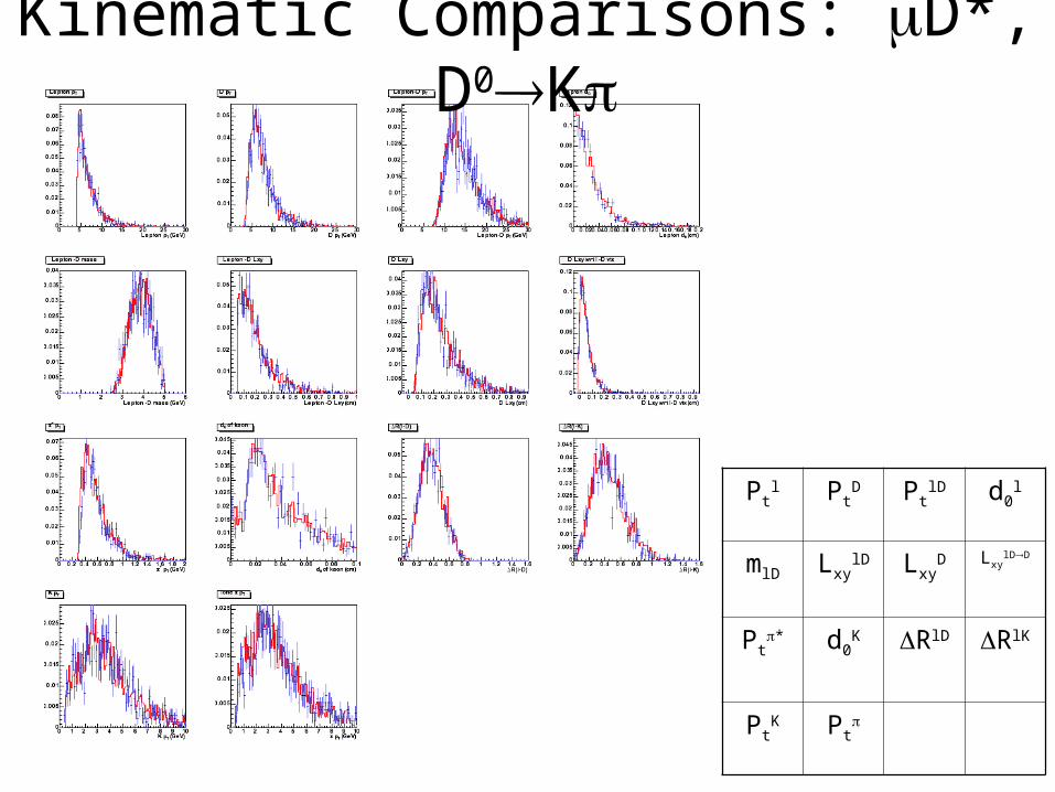
Kinematic Comparisons: D*, D0K

Ptl Pt

D PtlD d0

l

mlD LxylD Lxy

D LxylDD

Pt* d0

K RlD RlK

PtK Pt

Matching-2 prob (%)

K K(0) K K

e e e e

pT(l) 4 12 43 40 38 11 16 1

pT(D) 3 7 8 2 6 79 12 4

pT(l-D) 41 17 30 2 49 22 9 4

d0(l) 10 92 75 27 30 4 95 2

m(l-D) 2 3 50 61 48 69 16 42

LXY(l-D) 48 23 41 12 32 69 29 0.07

LXY(D) 23 88 69 99 95 47 87 2

LXY(B to D) 61 29 6 13 17 89 24 2

pT(*) >0.4

GeV

28 42 21 70 38 1 – –

do(K) 68 72 83 54 74 15 17 72

R(l-D) 34 29 26 51 86 33 57 30

R(l-K) 17 12 33 66 38 2 29 2

pT(K) 22 20 49 52 83 10 25 15

pT() 90 20 14 59 2 8 – –

pT(2) – – – – – – 67 64

Can we “predict” relative yields?

Two methods (a,b) to derive this BR

a) Based on inclusive bD(*)+l

b) Based on exclusive BD(*)+l, D**l

+PDG BR + MC efficiency ratios

Assume MC predictions and use 13% systematics

D**

Add another

**D**

Optimization• The relevant discriminants are:

– Pt

R– d0

PV

– d0BV

– d0DV

– LxyBD

• Signal model: MC• Background model:

– WS **l charge

• Optimize significance

PV

BVDV

**D0

D+

d0PV

d0BV

d0DV

Discriminating Variables

** Pt (GeV)

R (**-lD)

** 2d IP signif.WRT PV

** 3d IP signif.WRT BV

** 3d IP signif.WRT DV

Optimization!•Generate D** montecarlo (the shape)•Normalize D** MC to data with reasonable cuts•Now we can turn the crank and optimize…

But what?

)SB-(SB*a + )SB+(SB*a +S*2 + S WSRSWSRS2

WS

SS

bin

•a is the ratio of background events between signal and sideband region (a<1, usually)•S is the MC signal (right sign combinations, signal region)•SWS is the WS data in the signal region•SBRS is the RS data in the sideband region•SBWS is the WS data in the sideband region

Optimal point:

•We have to live with different selections for D**D+ and D**D*(K)

•Pt(**)>0.4 GeV

R<1.0–|d0

PV/|>2.5–|d0

BV/|<3.0

•S/sqrt(…)8D*

D+

• |d0DV/|>0.8

– Lxy(BD)>0.05 cm•S/sqrt(…)6.6

m**

Measure

<m**2>,

<m**4>

Current Mass Distributions

DELPHI:

~80 (K)

~80 (D+)

Background

Backgrounds• Background from B decays:

– Know how to model– Study using Bgenerator/EvtGen/TRGSim++/CdfSim

• “Feeddown”• Combinatorial background under D peaks:

– side-band subtraction

• Prompt pions in D(*)+-l-:– Mostly from fragmentation– wrong-sign combination D++l-

• cc– D0 impact parameter distribution

Physics Background

• Physics background studied with BD(*)+Ds

-

• Size wrt signal:

• 100% uncertainty

5.1

(*)

signalBBR

DDBBRlXDBR s

s

~7%

~7%~1

Other modes

Background: Feed Down

• Irreducible D**0 D*+( D+0)- background to

D**0 D+- subtracted statistically:

– M shape of D+- combination above is like D0-

from D**0 D*+( D0+)- – Rate is one half (isospin) times the relative

efficiency in both channels time the ratio of the D0 and D+ B.R.’s used in the analysis

2

10

KDBR

KDBR

K

K

Pollution from ccbar?•We are cutting hard on Lxy(B) (500m), this is known to “solve” the lifetime problem

•Look at D+/D0 impact parameter for evidence of prompt objects: we do not see any

Efficiency Corrections

Measure

<m**2>,

<m**4>

• Theory prediction depends on Pl* cuts. We cannot do much but:

– see how our efficiency as a function of Pl* looks like

– Use a threshold-like correction– Evaluate systematics for different threshold values

Pl*

MC efficiencies(M) is dependent on:

•D** decay Model

•Pl* cut

•Use different models/cuts to evaluate systematics:

•Individual resonances

•Goity-Roberts

•Phase space (not shown)

•Baseline: BR weighted

(EvtGen) average of modes

Corrections to MC efficiencies

• Worried about possible shortcomings of the MC simulation:– Efficiency for requiring Si hits ** separation variables not perfectly

reproduced by MC

• Use * candidates from data to derive corrections

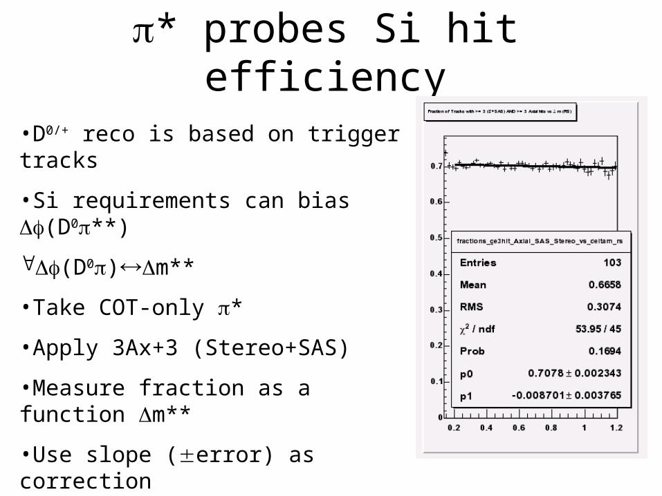
* probes Si hit efficiency

•D0/+ reco is based on trigger tracks

•Si requirements can bias (D0**)

(D0)m**

•Take COT-only *

•Apply 3Ax+3 (Stereo+SAS)

•Measure fraction as a function m**

•Use slope (error) as correction

** Separation Variables

124/49 137/43

146/45•Data MC comparison

•Behavior is similar, but there are discrepancies

•Derive corrections from this comparison

Data vs MC efficiencies•Apply to * the same tracking requirements we usually apply to ** (including Si hits)

•Measure efficiencies for ** selection cuts applied to *

•Take the ratio of MC and Data efficiencies as a function of Pt

Moments ExtractionProcedure

Measure

<m**2>,

<m**4>

Computing the D** Moments

• All the pieces are put together in an unbinned procedure using weighted events

• Signal right sign (SRS) w = +1

• Signal wrong sign (SWS) w = -1

• Sideband right sign (SBRS) w = -ai

• Sideband wrong sign (SBWS) w = +ai

• Apply efficiency corrections: efficiencies are propagated on weights

W=w (aPt**+b)/[MC(m**)(cm**+d)]

More Backgrounds

• Feed-down pseudo-events are formed from the D0** mass in Kevents (in SRS,SWS,SBRS,SBWS). The weight is

• Physics background events are generated and assigned a weight

where =0.07 is the efficiency of the background relative to the signal. The weight is then corrected with the efficiency factor from MC.

2

1

KDBR

KDBR

K

Kww

back

Dss N

N

signalBBR

DDBBRlXDBRw

**(*)

1

D+, D*+ Relative Normalization

• Relative normalization of D* channels is irrelevant since they all have the same underlying M distribution.

• D+ channel has a different M distribution. All D+ events have their weights modified as:

• Systematics:– BR uncertainties from PDG (7%) ratio from studies on data (13%)

K

DKDBR

KDBRDDBR

N

N

K

KwW

*00*

)(

)()(

Resulting m** distribution

42

12

**2

22**1

49.085.0

15.073.5

GeVmmm

GeVmm

D

D

Computing the Xc Moments

• The D0 and D*0 pieces have to be added to the D**0 moments, according to

where the fi are the fractions of Dil events above the pl*cut. Only ratios of fi’s enter the final result.

f

Moments ExtractionSystematics

Measure

<m**2>,

<m**4>

Systematicsshopping list

• Mass scale and resolution• Efficiency corrections

– From MC– from data

• Lepton momentum cut• Background model• Radial excitations• Physics background• Relative D+/D* normalization• Semileptonic B branching ratios• D** mass cut

Mass scale/resolution

• We are measuring m** and then adding the PDG masses for D+/D*Basically insensitive to absolute scale issuesMass resolution mattersThe sample with the worst resolution is K0

Re-smear K0 with 60MeV gaussian and use this as systematic

Efficiency corrections from MC•Uncertainty comes from lack of knowledge on the D** BR and phase space structures…

•Two possible MC models:

•BR weighted EvtGen admixture, to the best of today’s knowledge

•Plain phase space

•Switch to evaluate

systematics…

Efficiency Corrections from data

•Efficiencies measured on data have modeling uncertainties/stat. Errors

•Float parameters within ranges and compute the effect on the moments

•Mass-dependent: use stat error on slope

•Pt-dependent: use 0th/1st order polynomial difference

Lepton momentum cut-off

•We are not “literally” cutting on Pl* (it is not accessible, experimentally)•Detector implicitly cuts on it•Assume a baseline cut-off•Vary in a reasonable range to evaluate systematics

•We use f to derive f**, given f0, f*

•f=f(,1)

•We use experimental prior knowledge on ,1

to evaluate systematics

•Effect is negligible

Other Systematics

•Physics background:

–Branching ratios are poorly known (100% !!!)

•Relative BD/D*/D** branching ratios

•Take PDG values 1

•Theory parameters (1, i, S, mb, mc) varied according to expectations (100%, 0.5GeV3, 5%, 200MeV, 200 MeV)

back

Dss N

N

signalBBR

DDBBRlXDBRw

**(*)

1

•D+/D*+ relative scale:

•PDG BR are varied by 1

•MC based efficiencies 13%, according to studies in CDF6754 (D yields note)

Distribution Cut-off• The sample has basically no statistical power above

3.5 GeV (EvtGen predicts ~1% signal above cut)• We need to apply a cutoff in order not to

compromise the statistical uncertainty• Trade off:

– Drop the statistical error, but increase the size of systematics

– Becoming model dependent (we need a model for the extrapolation of the high tail in order to evaluate systematics)

Temporarily:

Evaluate moments with different cut-off (3.5-4.0)

Background Model• We have 2 possible problems

– Shape• Alternative model based on fully reconstructed B

(“embedding” work in progress)

– Scale• Based on the charge multiplicites from embedded

B+:– <20% discrepancy between RS and WS– ~20% of background comes from B+

~4% uncertainty on WS/RS scale

Radial Excitations

• D’D(*)+ should be accounted for in m**

• Not yet observed• DELPHI limits: • Embedding-WS comparison could

give another limit• For the time being we assume no D’

Systematics size

Results

• All systematics in place except the background shape model (embedding)

oror

Conclusions

• Comparison with other experiments

• Plan:– Embedding (background shape, D’)– Re-evaluate systematics on m**

cutoff at 3.5 GeV– Bless in 2 weeks

Backup Slides

Vcb: exclusive determination

• Measure absolute scale of BD*l• D** states also important for |Vcb|

exclusive determination– end-point in q2 for BD*l decays– systematic uncertainty from BD**l

background

Channels with neutral B

• B0 D**+ l-

– D**+ D0 + OK– D**+ D+ 0 Not reconstructed. Half the rate of D+ -

– D**+ D*0 +

• D*0 D0 0 Not reconstructed. Background to D0 +

• D*0 D0 Not reconstructed. Background to D0 +

– D**+ D*+ 0 Not reconstructed. Half the rate of D*+ -

We will not deal with neutral B

Data StabilityA: (152595-154012) Before winter 2003 shutdown

B: (158826-165297) After winter 2003 shutdown

C: (164303-165297) SVT 4/5

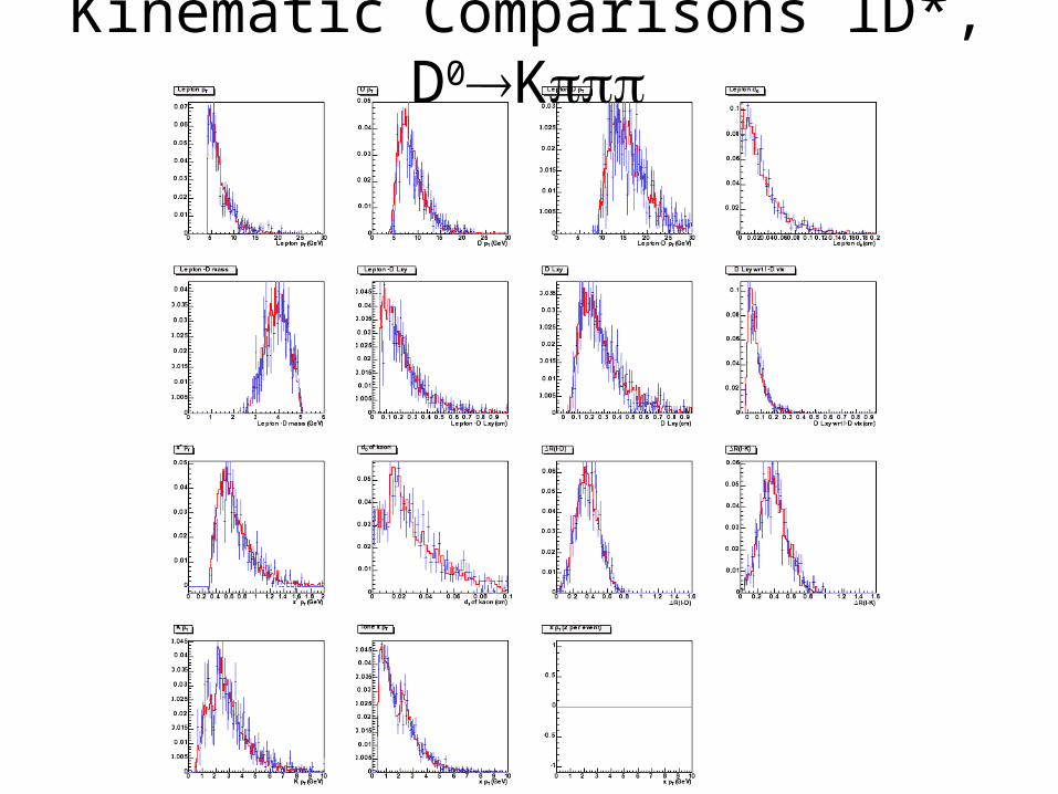
Kinematic Comparisons lD*, D0K

Kinematic Comparisons lD*, D0K0

Kinematic Comparisons: D+

Can we “predict” yields?

Two methods (a,b) to derive this BR

a) Based on inclusive bD(*)+l

b) Based on exclusive BD(*)+l, D**l

+PDG BR + MC efficiency ratios

What background model for what?

• WS is often used in this kind of analyses as a model for the background

• We can also use our fully reco’d B from other triggers

• We choose to use WS for the optimization

• Embedding is being used as a cross-check for systematics

D**D0

• No background subtraction

• ~80 events in D*+

• ~80 events in D+

• ~215 events on D0

uncertainty > sqrt(n)

What’s available on the market…D**D+

D**D*

Estimator Behaviour

K Optimization

D+ Optimization

Combinatorial Background• WS **

– Already used for the optimization– Physics can be different

• Fully reco. B– independent emulation of the background– Limited statistics– Needs some machinery for emulating a semileptonic decay!

• Eliminate the B daughters• Replace the B with a semileptonic B with the same 4-momentum:

a template montecarlo where the B decay comes from EvtGen and the rest of the event comes from the data!

Background Modeling II

Lxy>500m

•Tight cuts (avoid subtractions)

•Exclude B tracks

•Replace with MC B

•QuickCdfObjects/GenTrig

•Re-decay N times

•Same analysis path from there on

Signal Fits

Sample Consistency

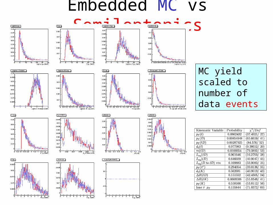
Embedded MC vs Semileptonics

MC yield scaled to number of data events

• Theory prediction depends on Pl* cuts. We cannot do much but:

– see how our analysis bias looks like– Use a threshold-like correction– Evaluate systematics for different threshold values

Pl*

MC efficiencies(M) is dependent on:

•D** decay Model

•Pl* cut

•Use different models/cuts to evaluate systematics

MC Validation* is an unique probe:

•Large statistics

•Low background

•“Similar” spectrum to **

•Can reconstruct with minimal cuts (e.g. COT only)

•Technique:

•Search for * with very loose cuts

•Do not include in B vertex

•Study biases to kinematics from tracking

•Study IP resolution(data/MC): Primary, B & D vertices

•Study (data/MC) vs selection criteria

MC validation•Cross-check kinematic variables

•B spectrum modeling

•Trigger emulation

•Validate CdfSim model of tracking resolution

•Relative efficiencies

** selection/bias•Compare many data/MC distributions using binned 2

•Every possible decay mode

•Sideband subtracted before comparison

•Duplicate removal (D0K)

Kinematics•Can we rely on kinematical biases estimated from MC?

•Rem: we don’t care about absolute scales

•Pt dependent MC/data ratio:

400 MeV

* Pt

MC

Data

MC/Data vs Pt

Impact Parameters148/34

26/30

151/45

134/32

61/30

118/43

40/33

42/42

58/52

Impact Parameters (covr)40/33

550/40

124/49

133/32

39/29

137/43

146/34

25/30

146/45

(MC), (data) vs selection criteria

Another perspective: MC(after/before) / data(after/before)

MC(after/before) / data(after/before)Plan for the evaluation of

systematics

Ds Background

•Use peak in D+ candidates to set the scale

•Measure the relative contribution of Ds decays to D+ fakes using MC

•Extrapolate to the total size of the contribution: 4%

•Build a suitable D** background model

•Subtract

Cross-feeds

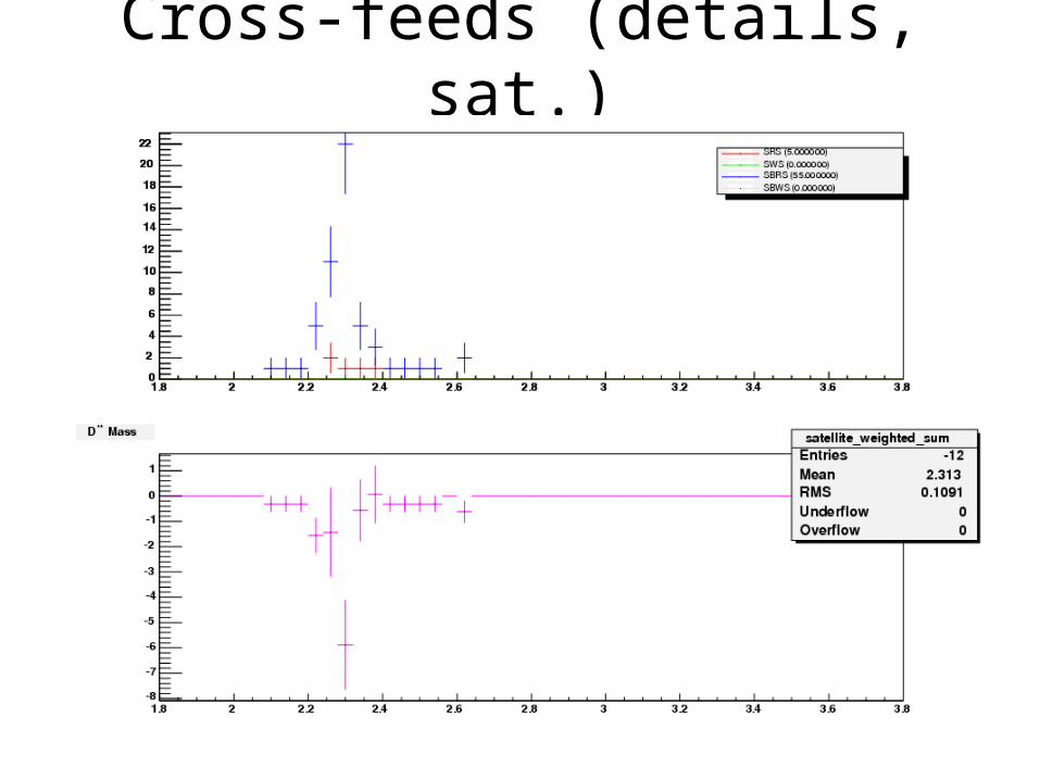
Cross-feeds (details, sat.)

Cross-feeds (details, K)

Cross-feeds (details K)

D** Moments

• Combine all events of all types in all channels (D*,D+,SRS,SBRS,feed-down, etc.)

• Compute mean (m1) and variance (m2) of M2 distribution with weighted events.

• Errors and correlation computed with MC (for toy MC) or bootstrap (for data).

• For some realizations, one finds a negative value for m2 = Var(M2) = <M4> - <M2>2.

Inputs for the D0 and D*0 Contributions

• For the BR’s, results from charged and neutral B decays are combined using isospin: partial widths are assumed equal.

• BR’s, ratio of lifetimes and ratio of production fractions are taken from PDG.

• Toy Monte Carlo is used to propagate the uncertainties from m1, m2, the BR’s, etc., to uncertainties on M1 and M2 and their correlation.