Embed Size (px)
Citation preview
Hamiltonian Multivector Fields and Poisson Formsin Multisymplectic Field Theory
Michael Forger 1 , Cornelius Paufler 2 and Hartmann Romer 3
1 Departamento de Matematica Aplicada,Instituto de Matematica e Estatıstica,
Universidade de Sao Paulo,Caixa Postal 66281,
BR–05315-970 Sao Paulo, S.P., Brazil
2 Matematisk Fysik / Alba NovaKungliga Tekniska HogskolanSE–10691 Stockholm, Sweden
3 Fakultat fur Mathematik und PhysikPhysikalisches Institut
Albert-Ludwigs-Universitat Freiburg im BreisgauHermann-Herder-Straße 3
D–79104 Freiburg i.Br., Germany
Abstract
We present a general classification of Hamiltonian multivector fields and ofPoisson forms on the extended multiphase space appearing in the geometricformulation of first order classical field theories. This is a prerequisite forcomputing explicit expressions for the Poisson bracket between two Poisson forms.
Universitat FreiburgTHEP 04/13
Universidade de Sao PauloRT-MAP-0402
July 2004
1E-mail address: [email protected] address: [email protected] address: [email protected]
1 Introduction and General Setup
The present paper is a continuation of previous work on Poisson brackets of differentialforms in the multiphase space approach to classical field theory [2, 3]. Our aim is tospecialize the general constructions of Ref. [3] from abstract (exact) multisymplecticmanifolds to the extended multiphase spaces of field theory, which at present seem tobe the only known examples of multisymplectic manifolds, to clarify the structure ofHamiltonian multivector fields, of Hamiltonian forms and of Poisson forms on thesespaces and to give explicit formulas for the Poisson bracket between the latter intro-duced in Refs [2, 3].
The structure of the article is as follows. In the remainder of this introduction,we briefly review the geometric constructions needed in the paper. We put particularemphasis on the consequences that arise from the existence of a certain vector field,the scaling or Euler vector field. Also, we fix the notation to be used in what follows.In Section 2, we present an explicit classification of locally Hamiltonian multivectorfields on extended multiphase space in terms of adapted local coordinates and, follow-ing the logical inclusion from locally Hamiltonian to (globally) Hamiltonian to exactHamiltonian multivector fields, show how the last two are situated within the first.Section 3 is devoted to the study of Hamiltonian forms and Poisson forms that areassociated with (globally) Hamiltonian multivector fields. In Section 4, we use theoutcome of our previous analysis to derive expressions for the Poisson bracket betweentwo Poisson forms. In Section 5, we summarize our main conclusions and commenton the relation of our results to other approaches, as well as on perspectives for futureresearch. Finally, in order to make the article self-contained, we include in an appendixa proposition that is not new but is needed in some of the proofs.
We begin with a few comments on the construction of the extended multiphase spaceof field theory [5–9], which starts out from a given general fiber bundle over space-time,with base space M (dim M = n), total space E, bundle projection π : E −→ Mand typical fiber Q (dim Q = N). It is usually referred to as the configuration bundlesince its sections constitute the possible field configurations of the system. (Of course,the manifold M represents space-time, whereas the manifold Q plays the role of aconfiguration space.) The extended multiphase space, which we shall simply denoteby P , is then the total space of a larger fiber bundle over M and in fact the totalspace of a vector bundle over E which can be defined in several equivalent ways, e.g.,by taking the twisted affine dual J©?E of the first order jet bundle JE of E or bytaking the bundle
∧nn−1T
∗E of (n− 1)-horizontal n-forms on E; see [3,7,9] for details.Therefore, there is a natural class of local coordinate systems on P , namely those thatarise from combining fiber bundle charts of E over M with vector bundle charts of Pover E: these so-called adapted local coordinates (xµ, qi, pµ
i , p) are completely fixed byspecifying local coordinates xµ for M (the space-time coordinates), local coordinates qi
for Q (the position variables) and a local trivialization of E over M , and are such thatthe induced local coordinates pµ
i (the multimomentum variables) and p (the energy
2

variable) are linear along the fibers of P over E. For details, we refer to Ref. [3], whereone can also find the explicit transformation law for the multimomentum variables andthe energy variable induced by a change of the space-time coordinates, of the positionvariables and of the local trivialization.
A first important feature of the extended multiphase space P is that it carries anaturally defined multicanonical form θ whose exterior derivative is, up to a sign, themultisymplectic form ω :
ω = − dθ . (1)
The global construction can be found in Refs [3,7,9], so we shall just state their explicitform in adapted local coordinates:
θ = pµi dqi ∧ dnxµ + p dnx . (2)
ω = dqi ∧ dpµi ∧ dnxµ − dp ∧ dnx . (3)
Here, we have already employed part of the following conventions concerning localdifferential forms defined by a system of adapted local coordinates, which will be usedsystematically throughout this paper:
dnx = dx1 ∧ . . . ∧ dxn , dnxµ1...µr= i∂µr
. . . i∂µ1dnx .
For later use, we also recall the definition of the Lie derivative of a differential form αalong an r-multivector field X,
LXα = d iXα − (−1)r iX dα , (4)
which leads to the following relations, valid for any differential form α and any twomultivector fields X and Y of tensor degrees r and s, respectively,
dLXα = (−1)r−1 LX dα , (5)
i[X,Y ]α = (−1)(r−1)s LXiY α − iY LXα , (6)
L[X,Y ]α = (−1)(r−1)(s−1) LXLY α − LY LXα , (7)
LX∧Y α = (−1)s iY LXα + LY iXα , (8)
where [X,Y ] denotes the Schouten bracket of X and Y . For decomposable multivectorfields X = X1 ∧ . . . ∧Xr and Y = Y1 ∧ . . . ∧Ys, it can be defined in terms of the Liebracket of vector fields according to the formula
[X,Y ] =r∑
i=1
s∑j=1
(−1)i+j [Xi, Xj] ∧X1 ∧ . . . Xi . . . ∧Xr ∧Y1 ∧ . . . Yj . . . ∧Ys ,
where as usual the hat over a symbol denotes its omission. We shall also write
LXY = [X, Y ] ,
3
for any two multivector fields X and Y . For properties of the Schouten bracket, werefer to [10]. A proof of the above identities relating the Schouten bracket and the Liederivative of forms along multivector fields can be found in the appendix of Ref. [3].
A second property of the extended multiphase space P which provides additionalstructures for tensor calculus on this manifold is that it is the total space of a fiberbundle, which implies that we may speak of vertical vectors and horizontal covectors. Infact, it is so in no less than three different ways. Namely, P is the total space of a fiberbundle over M (with respect to the so-called source projection), the total space of avector bundle over E (with respect to the so-called target projection) and the total spaceof an affine line bundle over the ordinary multiphase space P0 [3]. Therefore, the notionsof verticality for multivector fields and of horizontality for differential forms on P admitdifferent interpretations, depending on which projection is used. In any case, one startsby defining tangent vectors to the total space of a fiber bundle to be vertical if they areannihilated by the tangent map to the bundle projection, or what amounts to the samething, if they are tangent to the fibers. Dually, a k-form on the total space of a fiberbundle is said to be l-horizontal if it vanishes whenever one inserts at least k − l + 1vertical tangent vectors; the standard horizontal forms are obtained by taking l = k.Finally, an r-multivector on the total space of a fiber bundle is said to be s-verticalif its contraction with any (r − s + 1)-horizontal form vanishes. It is not difficult toshow that these definitions are equivalent to requiring that, locally, an l-horizontal k-form should be a sum of exterior products of k one-forms, among which there are atleast l horizontal ones, and that an s-vertical r-multivector field should be a sum ofexterior products of r tangent vectors, among which there are at least s vertical ones.Using this rule, properties of verticality for multivectors or horizontality for forms areeasily derived from the corresponding properties for vectors or one-forms, respectively.In what follows, the terms “vertical” and “horizontal” will usually refer to the sourceprojection, except when explicitly stated otherwise.
A third important feature of the extended multiphase space P is that it carries anaturally defined vector field Σ, the scaling vector field or Euler vector field, whichexists on any manifold that is the total space of a vector bundle. In adapted localcoordinates,
Σ = pµi
∂
∂pµi
+ p∂
∂p.
Obviously, we have iΣω = −θ. It is then easy to verify the following relations (seeProposition 2.1 of Ref. [3]):
LΣθ = θ , LΣω = ω . (9)
The main utility of Σ is that taking the Lie derivative LΣ along Σ provides a devicefor controlling the dependence of functions and, more generally, of tensor fields on Pon the multimomentum variables and the energy variable, that is, along the fibers of Pover E: LΣ has only integer eigenvalues, and eigenfunctions of LΣ with eigenvalue kare homogeneous polynomials of degree k in these variables.
4
As we shall see soon, homogeneity under LΣ plays a central role in the analysis ofvarious classes of multivector fields and differential forms on P .
Let us recall a few definitions. An r-multivector field X on P is called locallyHamiltonian if iXω is closed, or equivalently, if
LXω = 0 . (10)
It is called globally Hamiltonian if iXω is exact, that is, if there exists an (n− r)-formf on P such that
iXω = df . (11)
In this case, f is said to be a Hamiltonian form associated with X. Finally, it is calledexact Hamiltonian if
LXθ = 0 . (12)
Of course, exact Hamiltonian multivector fields are globally Hamiltonian (to show this,set f = (−1)r−1iXθ and apply eqs (4) and (1)), and globally Hamiltonian multivectorfields are obviously locally Hamiltonian. Conversely, an (n − r)-form f on P is calleda Hamiltonian form if there exists an r-multivector field X on P such that eq. (11)holds; in this case, X is said to be a Hamiltonian multivector field associated with f .Moreover, f is called a Poisson form if in addition, it vanishes on the kernel of ω, thatis, if for any multivector field Z, we have
iZ ω = 0 =⇒ iZf = 0 . (13)
A trivial example of a Poisson form is the multisymplectic form ω itself. Anotherexample is provided by the multicanonical form θ, since it can be written as θ = −iΣω.
Concerning stability under the Lie derivative along the scaling vector field Σ, wehave the following
Proposition 1.1 The space X∧LH(P ) of locally Hamiltonian multivector fields, the
space X∧H(P ) of globally Hamiltonian multivector fields, the space X∧
EH(P ) of exactHamiltonian multivector fields and the space X∧
0 (P ) of multivector fields taking valuesin the kernel of ω are all invariant under the Lie derivative along the scaling vectorfield Σ:
LXω = 0 =⇒ L[Σ,X]ω = 0 , (14)
iXω = df =⇒ i[Σ,X]ω = d (LΣf − f) , (15)
5
LXθ = 0 =⇒ L[Σ,X]θ = 0 , (16)
iξω = 0 =⇒ i[Σ,ξ]ω = 0 . (17)
Proof. All these relations can be shown by direct calculation.
Dually, we have
Proposition 1.2 The space ΩH(P ) of Hamiltonian forms, the space Ω0(P ) of formsthat vanish on the kernel of ω and the space ΩP (P ) of Poisson forms are all invariantunder the Lie derivative along the scaling vector field Σ:
df = iXω =⇒ d (LΣf) = iX+[Σ,X]ω . (18)
Proof. The first statement is a consequence of eq. (18), which follows directly fromcombining eqs (5) and (6) with eq. (9). For the second statement, assume that fvanishes on the kernel of ω. Then if ξ is any multivector field ξ taking values in thekernel of ω, the multivector field [Σ, ξ] takes values in the kernel of ω as well (cf.eq. (17)), so that according to eq. (6),
iξ (LΣf) = LΣiξf − i[Σ,ξ]f = 0 .
But this means that LΣf vanishes on the kernel of ω. Finally, the third statementfollows by combining the first two.
A special class of multivector fields and of differential forms on P which will be ofparticular importance in what follows is that of fiberwise polynomial multivector fieldsand of fiberwise polynomial differential forms on P : their coefficients are polynomialsalong the fibers of P over E, or in other words, polynomials in the multimomentumvariables and the energy variable. The main advantage of working with tensor fieldson the total space of a vector bundle which are fiberwise polynomial is that they allowa unique and globally defined (or in other words, coordinate independent) decompo-sition into homogeneous components, according to the different eigenspaces of the Liederivative LΣ along Σ; the corresponding eigenvalue will in what follows be called thescaling degree (to distinguish it from the ordinary tensor degree). In doing so, it mustbe borne in mind that, in an expansion with respect to an adapted local coordinatesystem, the scaling degree receives contributions not only from the coefficient functionsbut also from some of the coordinate vector fields and differentials since the vectorfields ∂/∂xµ, ∂/∂qi, ∂/∂pµ
i and ∂/∂p carry scaling degree 0, 0, −1 and −1, respec-tively, while the differentials dxµ, dqi, dpµ
i and dp carry scaling degree 0, 0, +1 and +1,respectively; moreover, the scaling degree is additive under the exterior product, sinceLΣ is a derivation. Therefore, a fiberwise polynomial r-multivector field on P admits aglobally defined decomposition into a finite sum
X =∑s>−r
Xs ,
6
where Xs is its homogeneous component of scaling degree s:
LΣXs = s Xs .
Each Xs can be obtained from X by applying a projector which is itself a polynomialin LΣ:
Xs =∏
s′>−r
s′ 6=s
1
s−s′(LΣ − s′) X .
Similarly, a fiberwise polynomial (n− r)-form f on P admits a globally defined decom-position into a finite sum
f =∑s>0
fs ,
where fs is its homogeneous component of scaling degree s:
LΣfs = s fs .
Again, the fs can be obtained from f :
fs =∏s′>0
s′ 6=s
1
s−s′(LΣ − s′) f .
The relevance of these decompositions for locally Hamiltonian multivector fields andfor Hamiltonian forms on the extended multiphase space P stems from the followingtheorem, whose proof will follow from statements to be derived in the course of thenext two sections, by means of explicit calculations in adapted local coordinates. Morespecifically, we have:
Theorem 1.3 Except for trivial contributions (multivector fields in the kernel of ωand closed differential forms, respectively), locally Hamiltonian multivector fields andHamiltonian forms on P are fiberwise polynomial. In particular, locally Hamiltonian r-multivector fields and Hamiltonian forms of degree n− r have non-trivial homogeneouscomponents of scaling degree s only for s = −1, 0, . . . , r − 1 and for s = 0, 1, . . . , r ,respectively. More precisely, we have:
• Every fiberwise polynomial locally Hamiltonian (Hamiltonian, exact Hamiltonian)r-multivector field X on P , with 0 < r < n, admits a unique, globally defineddecomposition into homogeneous components with respect to scaling degree, whichcan be written in the form1
X = X− + X+ + ξ with X+ =r−1∑s=0
Xs , (19)
1We abbreviate X−1 as X−.
7
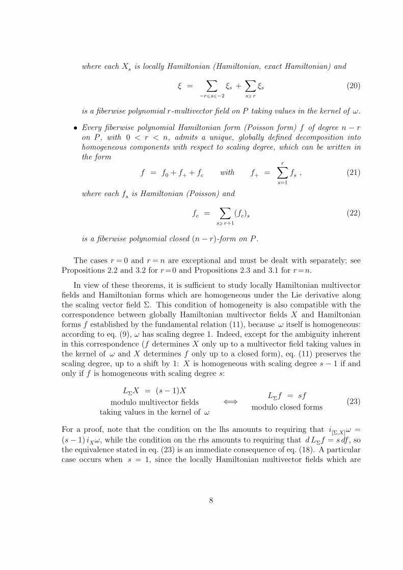
where each Xs is locally Hamiltonian (Hamiltonian, exact Hamiltonian) and
ξ =∑
−r6s6−2
ξs +∑s> r
ξs (20)
is a fiberwise polynomial r-multivector field on P taking values in the kernel of ω.
• Every fiberwise polynomial Hamiltonian form (Poisson form) f of degree n − ron P , with 0 < r < n, admits a unique, globally defined decomposition intohomogeneous components with respect to scaling degree, which can be written inthe form
f = f0 + f+ + fc with f+ =r∑
s=1
fs , (21)
where each fs is Hamiltonian (Poisson) and
fc =∑
s> r+1
(fc)s (22)
is a fiberwise polynomial closed (n− r)-form on P .
The cases r = 0 and r = n are exceptional and must be dealt with separately; seePropositions 2.2 and 3.2 for r=0 and Propositions 2.3 and 3.1 for r=n.
In view of these theorems, it is sufficient to study locally Hamiltonian multivectorfields and Hamiltonian forms which are homogeneous under the Lie derivative alongthe scaling vector field Σ. This condition of homogeneity is also compatible with thecorrespondence between globally Hamiltonian multivector fields X and Hamiltonianforms f established by the fundamental relation (11), because ω itself is homogeneous:according to eq. (9), ω has scaling degree 1. Indeed, except for the ambiguity inherentin this correspondence (f determines X only up to a multivector field taking values inthe kernel of ω and X determines f only up to a closed form), eq. (11) preserves thescaling degree, up to a shift by 1: X is homogeneous with scaling degree s − 1 if andonly if f is homogeneous with scaling degree s:
LΣX = (s− 1)X
modulo multivector fieldstaking values in the kernel of ω
⇐⇒LΣf = sf
modulo closed forms(23)
For a proof, note that the condition on the lhs amounts to requiring that i[Σ,X]ω =
(s− 1) iXω, while the condition on the rhs amounts to requiring that dLΣf = s df , sothe equivalence stated in eq. (23) is an immediate consequence of eq. (18). A particularcase occurs when s = 1, since the locally Hamiltonian multivector fields which are
8
homogeneous of scaling degree 0 are precisely the exact Hamiltonian multivector fields:for LXω = 0,
LΣX = 0
modulo multivector fieldstaking values in the kernel of ω
⇐⇒ LXθ = 0 . (24)
Indeed, the properties of θ and ω give
LXθ = −LXiΣω = (−1)r(i[X,Σ]ω − iΣLXω
)= (−1)r−1 i[Σ,X]ω . (25)
More generally, the fundamental relation (11) preserves the property of being fiber-wise polynomial, in the following sense: If X is a fiberwise polynomial Hamiltonianr-multivector field and f is a Hamiltonian (n− r)-form associated with X, then modi-fying f by addition of an appropriate closed (n− r)-form if necessary, we may alwaysassume, without loss of generality, that f is fiberwise polynomial as well. Conversely,if f is a fiberwise polynomial Hamiltonian (n − r)-form and X is a Hamiltonian r-multivector field associated with f , then modifying X by addition of an appropriater-multivector field taking values in the kernel of ω if necessary, we may always assume,without loss of generality, that X is fiberwise polynomial as well.
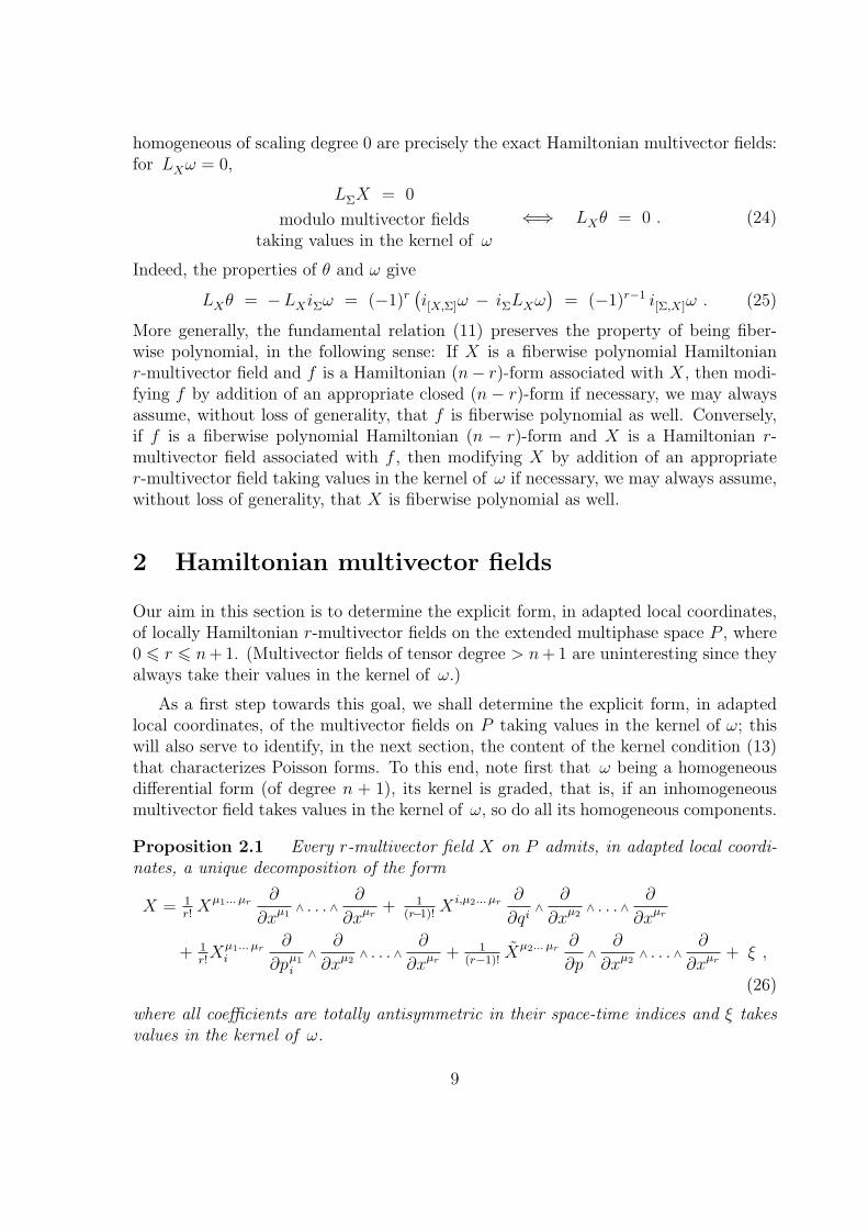
2 Hamiltonian multivector fields
Our aim in this section is to determine the explicit form, in adapted local coordinates,of locally Hamiltonian r-multivector fields on the extended multiphase space P , where0 6 r 6 n + 1. (Multivector fields of tensor degree > n + 1 are uninteresting since theyalways take their values in the kernel of ω.)
As a first step towards this goal, we shall determine the explicit form, in adaptedlocal coordinates, of the multivector fields on P taking values in the kernel of ω; thiswill also serve to identify, in the next section, the content of the kernel condition (13)that characterizes Poisson forms. To this end, note first that ω being a homogeneousdifferential form (of degree n + 1), its kernel is graded, that is, if an inhomogeneousmultivector field takes values in the kernel of ω, so do all its homogeneous components.
Proposition 2.1 Every r-multivector field X on P admits, in adapted local coordi-nates, a unique decomposition of the form
X = 1r!
Xµ1... µr∂
∂xµ1∧ . . . ∧
∂
∂xµr+ 1
(r−1)!X i,µ2... µr
∂
∂qi∧
∂
∂xµ2∧ . . . ∧
∂
∂xµr
+ 1r!Xµ1... µr
i
∂
∂pµ1
i
∧∂
∂xµ2∧ . . . ∧
∂
∂xµr+ 1
(r−1)!Xµ2... µr
∂
∂p∧
∂
∂xµ2∧ . . . ∧
∂
∂xµr+ ξ ,
(26)
where all coefficients are totally antisymmetric in their space-time indices and ξ takesvalues in the kernel of ω.
9

Proof. This is an immediate consequence of the particular form of ω in adaptedcoordinates, eq. (3), cf. [4].
With the standard local coordinate representation (26) for r-multivector fields X athand, we are now in a position to analyze the restrictions imposed on the coefficientsXµ1... µr , X i,µ2... µr , Xµ1... µr
i and Xµ2... µr by requiring X to be locally Hamiltonian.2
As a warm-up exercise, we shall settle the extreme cases of tensor degree 0 and n + 1.
Proposition 2.2 A function on P , regarded as a 0-multivector field, is locally Hamil-tonian if and only if it is constant; it is then also exact Hamiltonian. Similarly, an(n + 1)-multivector field on P , with standard local coordinate representation
X = X∂
∂p∧
∂
∂x1∧ . . . ∧
∂
∂xn+ ξ , (27)
where ξ takes values in the kernel of ω, is locally Hamiltonian if and only if the coeffi-cient function X is constant and is exact Hamiltonian if and only if it vanishes.
Proof. For functions, we use the fact that the operator i1 corresponding to the con-stant function 1 on a manifold is defined to be the identity, so that the operator ifcorresponding to an arbitrary function f on a manifold is simply multiplication by f .Therefore, we have for any differential form α
Lf α = d(if α)− if dα = d (fα) − f dα = df ∧α ,
implying that if f is constant, Lfα = 0 no matter what α one chooses. Similarly, formultivector fields of degree n + 1, it is clear that, as r equals n + 1, the first threeterms in eq. (26) also take values in the kernel of ω and can thus be incorporated intoξ. Therefore, by putting Xµ1... µn = εµ1... µnX, we see that iXω = −X. But LXω =d(iXω) − (−1)n iXdω = d(iXω) and LXθ = d(iXθ) − (−1)n+1 iXdθ = (−1)n+1 iXω,so the proposition follows.
The intermediate cases (0 < r 6 n) are much more interesting. However, thesituation for tensor degree n is substantially different from that for tensor degree < n,mainly due to the fact that when r equals n, the first term in eq. (26) lies in the kernelof ω. This case is off the main treatment below, so it will be dealt with first. To simplifythe notation, we write
Xµ1... µn = εµ1... µn X, X i,µ2... µn = εµ2... µnµ X iµ,
Xµ1... µn
i = εµ1... µn Xi, Xµ2... µn = εµ2... µnµ Xµ,
so that we obtain
iXω = (−1)n−1 X dp + X iµ dpµ
i − (−1)n−1 Xi dqi − Xµ dxµ , (28)
2Of course, it makes no sense to discuss the question which locally Hamiltonian multivector fieldsare also globally Hamiltonian when working in local coordinates.
10
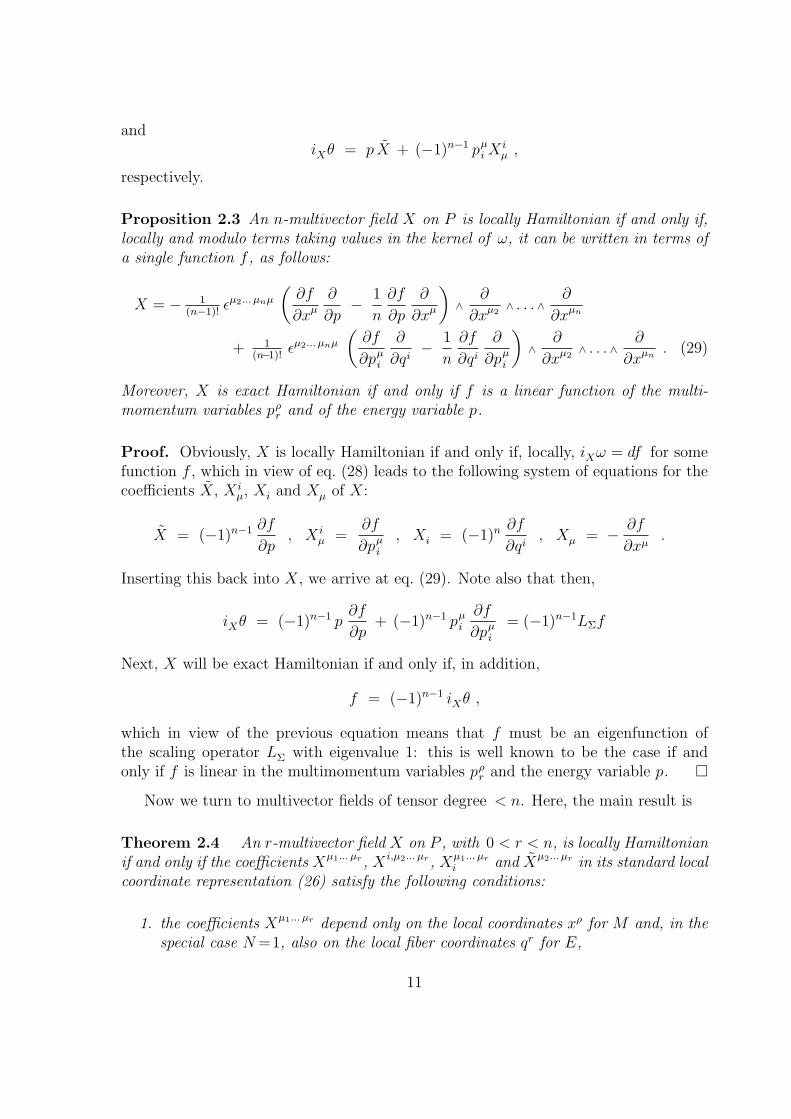
andiXθ = p X + (−1)n−1 pµ
i Xiµ ,
respectively.
Proposition 2.3 An n-multivector field X on P is locally Hamiltonian if and only if,locally and modulo terms taking values in the kernel of ω, it can be written in terms ofa single function f , as follows:
X = − 1(n−1)!
εµ2... µnµ
(∂f
∂xµ
∂
∂p− 1
n
∂f
∂p
∂
∂xµ
)∧
∂
∂xµ2∧ . . . ∧
∂
∂xµn
+ 1(n−1)!
εµ2... µnµ
(∂f
∂pµi
∂
∂qi− 1
n
∂f
∂qi
∂
∂pµi
)∧
∂
∂xµ2∧ . . . ∧
∂
∂xµn. (29)
Moreover, X is exact Hamiltonian if and only if f is a linear function of the multi-momentum variables pρ
r and of the energy variable p.
Proof. Obviously, X is locally Hamiltonian if and only if, locally, iXω = df for somefunction f , which in view of eq. (28) leads to the following system of equations for thecoefficients X, X i
µ, Xi and Xµ of X:
X = (−1)n−1 ∂f
∂p, X i
µ =∂f
∂pµi
, Xi = (−1)n ∂f
∂qi, Xµ = − ∂f
∂xµ.
Inserting this back into X, we arrive at eq. (29). Note also that then,
iXθ = (−1)n−1 p∂f
∂p+ (−1)n−1 pµ
i
∂f
∂pµi
= (−1)n−1LΣf
Next, X will be exact Hamiltonian if and only if, in addition,
f = (−1)n−1 iXθ ,
which in view of the previous equation means that f must be an eigenfunction ofthe scaling operator LΣ with eigenvalue 1: this is well known to be the case if andonly if f is linear in the multimomentum variables pρ
r and the energy variable p.
Now we turn to multivector fields of tensor degree < n. Here, the main result is
Theorem 2.4 An r-multivector field X on P , with 0 < r < n, is locally Hamiltonianif and only if the coefficients Xµ1... µr , X i,µ2... µr , Xµ1... µr
i and Xµ2... µr in its standard localcoordinate representation (26) satisfy the following conditions:
1. the coefficients Xµ1... µr depend only on the local coordinates xρ for M and, in thespecial case N =1, also on the local fiber coordinates qr for E,
11

2. the coefficients X i,µ2... µr are “antisymmetric polynomials in the multimomentumvariables” of degree r−1, i.e., they can be written in the form
X i,µ2... µr =r∑
s=1
X i,µ2... µr
s−1 , (30)
with
X i,µ2... µr
s−1 =1
(s−1)!
1
(r−s)!
∑π ∈Sr−1
(−1)π pµπ(2)
i2. . . p
µπ(s)
isY
ii2... is,µπ(s+1)... µπ(r)
s−1 , (31)
where Sr−1 denotes the permutation group of 2, . . . , r and the coefficientsY
ii2...is,µs+1...µr
s−1 depend only on the local coordinates xρ for M as well as the localfiber coordinates qr for E and are totally antisymmetric in i, i2, . . . , is as well asin µs+1, . . . , µr.
3. the remaining coefficients Xµ1... µr
i and Xµ2... µr can be expressed in terms of theprevious ones and of new coefficients Xµ1... µr
− depending only on the local coor-dinates xρ for M as well as the local fiber coordinates qr for E and are totallyantisymmetric in µ1, . . . , µr, according to
Xµ1... µr
i = − p∂Xµ1... µr
∂qi+ pµ
i
∂Xµ1... µr
∂xµ −r∑
s=1
pµs
i
∂Xµ1... µs−1νµs+1... µr
∂xν
− Σ−1
(r∑
s=1
(−1)s−1 pµs
j
∂Xj,µ1... µs−1µs+1... µr
∂qi
)+
∂Xµ1... µr−
∂qi,
(32)
(the first term being absent as soon as N > 1) and
Xµ2... µr = (−1)r p∂Xµ2... µrν
∂xν
− Σ−1
(pµ
i
∂X i,µ2... µr
∂xµ −r∑
s=2
pµs
i
∂Xi,µ2... µs−1νµs+1... µr
∂xν
)
− (−1)r ∂Xµ2... µrν−
∂xν.
(33)
It is exact Hamiltonian if and only if, in addition, the coefficents X i,µ2... µr depend onlyon the local coordinates xρ for M as well as the local fiber coordinates qr for E and thecoefficients Xµ1... µr
− vanish.
Proof. The proof will be carried out by “brute force” computation [4]. We obtain for
12
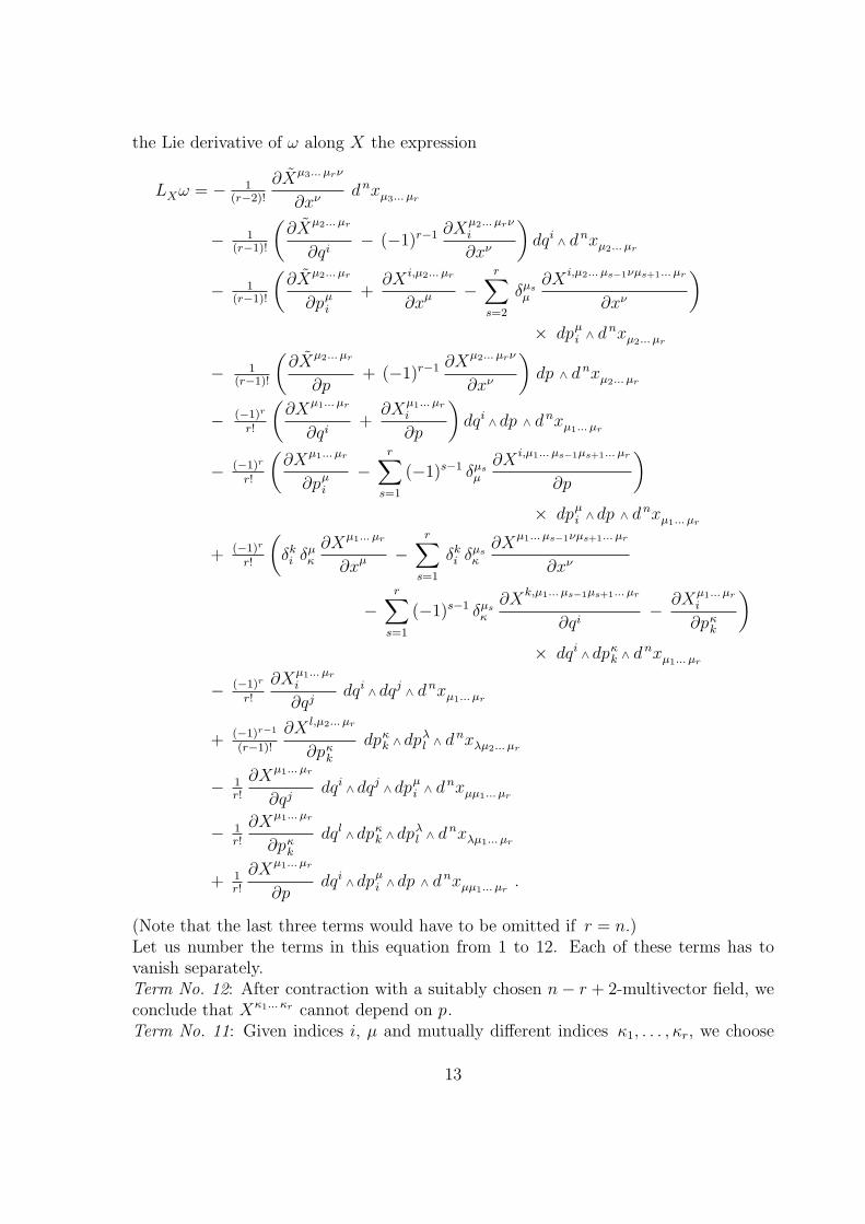
the Lie derivative of ω along X the expression
LXω = − 1(r−2)!
∂Xµ3... µrν
∂xνdnxµ3... µr
− 1(r−1)!
(∂Xµ2... µr
∂qi− (−1)r−1 ∂Xµ2... µrν
i
∂xν
)dqi ∧ dnxµ2... µr
− 1(r−1)!
(∂Xµ2... µr
∂pµi
+∂X i,µ2... µr
∂xµ −r∑
s=2
δµsµ
∂Xi,µ2... µs−1νµs+1... µr
∂xν
)× dpµ
i ∧ dnxµ2... µr
− 1(r−1)!
(∂Xµ2... µr
∂p+ (−1)r−1 ∂Xµ2... µrν
∂xν
)dp ∧ dnxµ2... µr
− (−1)r
r!
(∂Xµ1... µr
∂qi+
∂Xµ1... µr
i
∂p
)dqi ∧ dp ∧ dnxµ1... µr
− (−1)r
r!
(∂Xµ1... µr
∂pµi
−r∑
s=1
(−1)s−1 δµsµ
∂Xi,µ1... µs−1µs+1... µr
∂p
)× dpµ
i ∧ dp ∧ dnxµ1... µr
+ (−1)r
r!
(δki δµ
κ
∂Xµ1... µr
∂xµ −r∑
s=1
δki δµs
κ
∂Xµ1... µs−1νµs+1... µr
∂xν
−r∑
s=1
(−1)s−1 δµsκ
∂Xk,µ1... µs−1µs+1... µr
∂qi− ∂Xµ1... µr
i
∂pκk
)× dqi ∧ dpκ
k ∧ dnxµ1... µr
− (−1)r
r!
∂Xµ1... µr
i
∂qjdqi ∧ dqj ∧ dnxµ1... µr
+ (−1)r−1
(r−1)!
∂X l,µ2... µr
∂pκk
dpκk ∧ dpλ
l ∧ dnxλµ2... µr
− 1r!
∂Xµ1... µr
∂qjdqi ∧ dqj ∧ dpµ
i ∧ dnxµµ1... µr
− 1r!
∂Xµ1... µr
∂pκk
dql ∧ dpκk ∧ dpλ
l ∧ dnxλµ1... µr
+ 1r!
∂Xµ1... µr
∂pdqi ∧ dpµ
i ∧ dp ∧ dnxµµ1... µr.
(Note that the last three terms would have to be omitted if r = n.)Let us number the terms in this equation from 1 to 12. Each of these terms has tovanish separately.Term No. 12: After contraction with a suitably chosen n− r + 2-multivector field, weconclude that Xκ1... κr cannot depend on p.Term No. 11: Given indices i, µ and mutually different indices κ1, . . . , κr, we choose
13
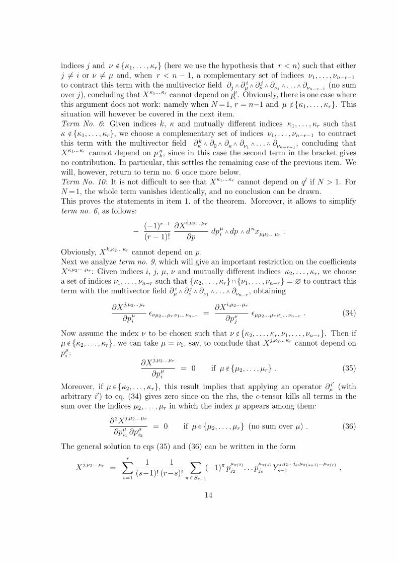
indices j and ν /∈ κ1, . . . , κr (here we use the hypothesis that r < n) such that eitherj 6= i or ν 6= µ and, when r < n − 1, a complementary set of indices ν1, . . . , νn−r−1
to contract this term with the multivector field ∂j ∧ ∂ iµ ∧ ∂ j
ν ∧ ∂ν1∧ . . . ∧ ∂νn−r−1
(no sumover j), concluding that Xκ1... κr cannot depend on pµi . Obviously, there is one case wherethis argument does not work: namely when N =1, r = n−1 and µ /∈ κ1, . . . , κr. Thissituation will however be covered in the next item.Term No. 6: Given indices k, κ and mutually different indices κ1, . . . , κr such thatκ /∈ κ1, . . . , κr, we choose a complementary set of indices ν1, . . . , νn−r−1 to contractthis term with the multivector field ∂ k
κ ∧ ∂0 ∧ ∂κ ∧ ∂ν1∧ . . . ∧ ∂νn−r−1
, concluding thatXκ1... κr cannot depend on p κ
k, since in this case the second term in the bracket givesno contribution. In particular, this settles the remaining case of the previous item. Wewill, however, return to term no. 6 once more below.Term No. 10: It is not difficult to see that Xκ1... κr cannot depend on ql if N > 1. ForN =1, the whole term vanishes identically, and no conclusion can be drawn.This proves the statements in item 1. of the theorem. Moreover, it allows to simplifyterm no. 6, as follows:
− (−1)r−1
(r − 1)!
∂X i,µ2... µr
∂pdpµ
i ∧ dp ∧ dnxµµ2... µr.
Obviously, Xk,κ2... κr cannot depend on p.Next we analyze term no. 9, which will give an important restriction on the coefficientsX i,µ2··· ,µr : Given indices i, j, µ, ν and mutually different indices κ2, . . . , κr, we choosea set of indices ν1, . . . , νn−r such that κ2, . . . , κr ∩ ν1, . . . , νn−r = ∅ to contract thisterm with the multivector field ∂ i
µ ∧ ∂ jν ∧ ∂ν1
∧ . . . ∧ ∂νn−r, obtaining
∂Xj,µ2... µr
∂pµi
ενµ2... µr ν1... νn−r =∂X i,µ2... µr
∂pνj
εµµ2... µr ν1... νn−r . (34)
Now assume the index ν to be chosen such that ν /∈ κ2, . . . , κr, ν1, . . . , νn−r. Then ifµ /∈ κ2, . . . , κr, we can take µ = ν1, say, to conclude that Xj,κ2... κr cannot depend onpµ
i :
∂Xj,µ2... µr
∂pµi
= 0 if µ /∈ µ2, . . . , µr . (35)
Moreover, if µ ∈ κ2, . . . , κr, this result implies that applying an operator ∂ i′µ (with
arbitrary i′) to eq. (34) gives zero since on the rhs, the ε-tensor kills all terms in thesum over the indices µ2, . . . , µr in which the index µ appears among them:
∂2Xj,µ2... µr
∂pµi1
∂pµi2
= 0 if µ ∈ µ2, . . . , µr (no sum over µ) . (36)
The general solution to eqs (35) and (36) can be written in the form
Xj,µ2... µr =r∑
s=1
1
(s−1)!
1
(r−s)!
∑π ∈Sr−1
(−1)π pµπ(2)
j2. . . p
µπ(s)
jsY
j,j2...js,µπ(s+1)...µπ(r)
s−1 ,
14

where Sr−1 denotes the permutation group of 2, . . . , r and the newly introducedcoefficients Y
i,j2...js,µs+1...µr
s−1 are local functions on E: they do not depend on the multi-momentum variables pκ
k or the energy variable p and are totally antisymmetric bothin j2, . . . , js and in µs+1, . . . , µr. Differentiating this expression with respect to pµ
i withµ = µ2 gives
∂Xj,µµ3... µr
∂pµi
ενµµ3... µr ν1... νn−r (no sum over µ)
=r∑
s=2
1(s−2)!
1(r−s)!
∑π ∈Sr−2
(−1)π pµπ(3)
j3. . . p
µπ(s)
jsY
j,ij3...js,µπ(s+1)...µπ(r)
s−1 ενµµ3... µr ν1... νn−r ,
where Sr−2 denotes the permutation group of 3, . . . , r, which shows that eq. (34) willhold provided that
Yj,ij3...js,µπ(s+1)...µπ(r)
s−1 = −Yi,jj3...js,µπ(s+1)...µπ(r)
s−1 .
This proves the statements in item 2. of the theorem.We proceed with terms no. 4 and 5 which imply
∂Xµ2... µr
∂p= (−1)r ∂Xµ2... µrν
∂xν,
∂Xµ1... µr
i
∂p= − ∂Xµ1... µr
∂qi. (37)
We observe first of all that the rhs of both equations does not depend on the energyvariable, so they can be immediately integrated with respect to p.From term no. 3 we infer
∂Xµ2... µr
∂pµi
= − ∂X i,µ2... µr
∂xµ +r∑
s=2
δµsµ
∂Xi,µ2... µs−1νµs+1... µr
∂xν. (38)
An explicit calculation shows that the rhs of this equation does not depend on the pµj ,
not only when µ /∈ µ2, . . . , µr but even when µ ∈ µ2, . . . , µr. (Of course, it alsodoes not depend on p.) Thus, according to lemma A.2 formulated in the appendix, wecan integrate eq. (38) explicitly to obtain3
Xµ2... µr = (−1)r p∂Xµ2... µrν
∂xν− Σ−1
(pµ
i
∂X i,µ2... µr
∂xµ −r∑
s=2
pµs
i
∂Xi,µ2... µs−1νµs+1... µr
∂xν
)+ Y µ2... µr , (39)
where the Y µ2... µr are local functions on E: they do not depend on the multimomentumvariables or on the energy variable.
3Recall that Σ−1 is the operator that acts on polynomials in the multimomentum variables and theenergy variable without constant term by multiplying the homogeneous component of degree s by 1/s.
15
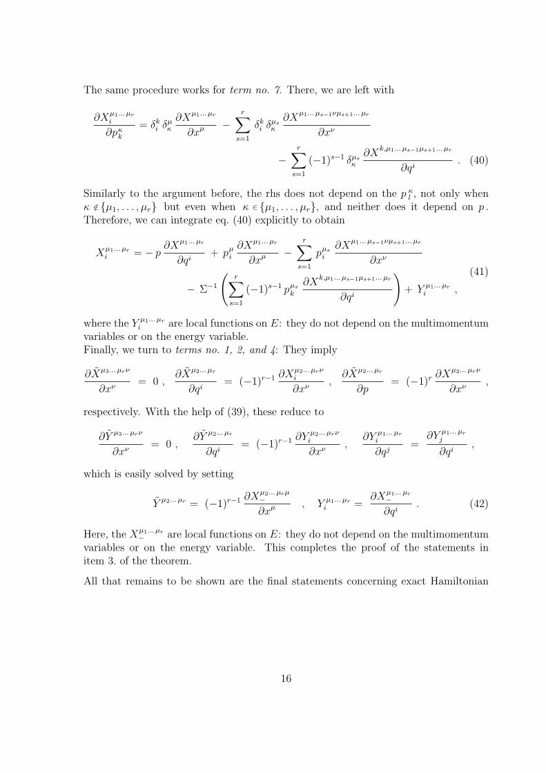
The same procedure works for term no. 7. There, we are left with
∂Xµ1... µr
i
∂pκk
= δki δµ
κ
∂Xµ1... µr
∂xµ −r∑
s=1
δki δµs
κ
∂Xµ1... µs−1νµs+1... µr
∂xν
−r∑
s=1
(−1)s−1 δµsκ
∂Xk,µ1... µs−1µs+1... µr
∂qi. (40)
Similarly to the argument before, the rhs does not depend on the p κl , not only when
κ /∈ µ1, . . . , µr but even when κ ∈ µ1, . . . , µr, and neither does it depend on p .Therefore, we can integrate eq. (40) explicitly to obtain
Xµ1... µr
i = − p∂Xµ1... µr
∂qi+ pµ
i
∂Xµ1... µr
∂xµ −r∑
s=1
pµs
i
∂Xµ1... µs−1νµs+1... µr
∂xν
− Σ−1
(r∑
s=1
(−1)s−1 pµs
k
∂Xk,µ1... µs−1µs+1... µr
∂qi
)+ Y µ1... µr
i ,
(41)
where the Y µ1... µr
i are local functions on E: they do not depend on the multimomentumvariables or on the energy variable.Finally, we turn to terms no. 1, 2, and 4: They imply
∂Xµ3... µrν
∂xν= 0 ,
∂Xµ2... µr
∂qi= (−1)r−1 ∂Xµ2... µrν
i
∂xν,
∂Xµ2... µr
∂p= (−1)r ∂Xµ2... µrν
∂xν,
respectively. With the help of (39), these reduce to
∂Y µ3... µrν
∂xν= 0 ,
∂Y µ2... µr
∂qi= (−1)r−1 ∂Y µ2... µrν
i
∂xν,
∂Y µ1... µr
i
∂qj=
∂Y µ1... µr
j
∂qi,
which is easily solved by setting
Y µ2... µr = (−1)r−1 ∂Xµ2... µrµ−
∂xµ , Y µ1... µr
i =∂Xµ1... µr
−
∂qi. (42)
Here, the Xµ1... µr− are local functions on E: they do not depend on the multimomentum
variables or on the energy variable. This completes the proof of the statements initem 3. of the theorem.
All that remains to be shown are the final statements concerning exact Hamiltonian
16
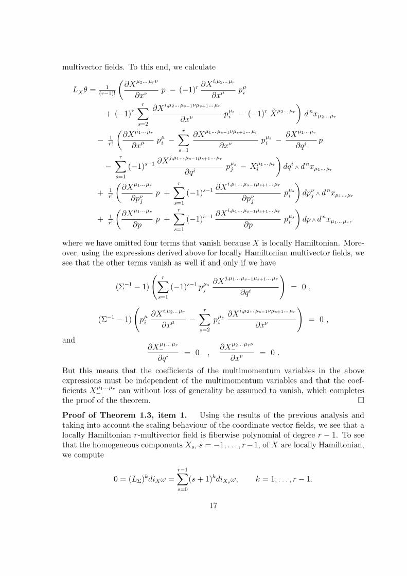
multivector fields. To this end, we calculate
LXθ = 1(r−1)!
(∂Xµ2... µrν
∂xνp − (−1)r ∂X i,µ2... µr
∂xµ pµi
+ (−1)r
r∑s=2
∂Xi,µ2... µs−1νµs+1... µr
∂xνpµs
i − (−1)r Xµ2... µr
)dnxµ2... µr
− 1r!
(∂Xµ1... µr
∂xµ pµi −
r∑s=1
∂Xµ1... µs−1νµs+1... µr
∂xνpµs
i − ∂Xµ1... µr
∂qip
−r∑
s=1
(−1)s−1 ∂Xj,µ1... µs−1µs+1... µr
∂qipµs
j − Xµ1... µr
i
)dqi ∧ dnxµ1... µr
+ 1r!
(∂Xµ1... µr
∂pνj
p +r∑
s=1
(−1)s−1 ∂Xi,µ1... µs−1µs+1... µr
∂pνj
pµs
i
)dpν
j ∧ dnxµ1... µr
+ 1r!
(∂Xµ1... µr
∂pp +
r∑s=1
(−1)s−1 ∂Xi,µ1... µs−1µs+1... µr
∂ppµs
i
)dp ∧ dnxµ1... µr ,
where we have omitted four terms that vanish because X is locally Hamiltonian. More-over, using the expressions derived above for locally Hamiltonian multivector fields, wesee that the other terms vanish as well if and only if we have
(Σ−1 − 1)
(r∑
s=1
(−1)s−1 pµs
j
∂Xj,µ1... µs−1µs+1... µr
∂qi
)= 0 ,
(Σ−1 − 1)
(pµ
i
∂X i,µ2... µr
∂xµ −r∑
s=2
pµs
i
∂Xi,µ2... µs−1νµs+1... µr
∂xν
)= 0 ,
and∂Xµ1... µr
−
∂qi= 0 ,
∂Xµ2... µrν−
∂xν= 0 .
But this means that the coefficients of the multimomentum variables in the aboveexpressions must be independent of the multimomentum variables and that the coef-ficients Xµ1... µr
− can without loss of generality be assumed to vanish, which completesthe proof of the theorem.
Proof of Theorem 1.3, item 1. Using the results of the previous analysis andtaking into account the scaling behaviour of the coordinate vector fields, we see that alocally Hamiltonian r-multivector field is fiberwise polynomial of degree r − 1. To seethat the homogeneous components Xs, s = −1, . . . , r−1, of X are locally Hamiltonian,we compute
0 = (LΣ)kdiXω =r−1∑s=0
(s + 1)kdiXsω, k = 1, . . . , r − 1.
17

Together with diXω = 0, this leads to a Vandermonde matrix equation with entries0, 2, 3, . . . , r− 1 annihilating the vector (diX−1ω, . . . , diXr−1)
T . As the determinant of aVandermonde matrix does not vanish, the above vector has to vanish.
The following proposition clarifies the interpretation of homogeneous locally Hamil-tonian multivector fields.
Proposition 2.5 Let X be a locally Hamiltonian r-multivector field on P . Then
1. X is exact Hamiltonian iff [Σ, X] takes values in the kernel of ω.
2. If [Σ, X]− sX takes values in the kernel of ω, for some integer s between 0 andr − 1, then X is globally Hamiltonian with associated Poisson form
(−1)r−1
s + 1iXθ .
3. If [Σ, X] + X takes values in the kernel of ω, then iXθ = 0.
Proof. The first statement follows immediately from eq. (25). Similarly, the secondclaim can be proved by multiplying eq. (25) by (−1)r−1/(s + 1) and combining it witheq. (1) and eq. (4) to give
d
((−1)r−1
s + 1iXθ
)=
(−1)r−1
s + 1LXθ +
1
s + 1iXω =
1
s + 1i[Σ,X]+X ω ,
which equals iXω since, by hypothesis, i[Σ,X]−sX ω = 0. Finally, the third statementfollows by observing that the kernel of ω is contained in the kernel of θ and henceaccording to the hypothesis made,
0 = i[Σ,X]+Xθ = LΣiXθ − iXLΣθ + iXθ = LΣiXθ ,
where we have used the invariance of θ under Σ. Therefore, according to Proposi-tion A.1, iXθ is the pull-back to P of an n-form on E via the projection that defines Pas a vector bundle over E, which in turn can be obtained as the pull back to E of iXθvia the zero section of P over E. But this pull-back is zero, since θ vanishes along thezero section of P over E.
It may be instructive to spell all this out more explicitly for locally Hamiltonianvector fields (r=1).
We begin by writing down the general form of a locally Hamiltonian vector field X:in adapted local coordinates, it has the representation
X = Xµ ∂
∂xµ + X i ∂
∂qi+ Xµ
i
∂
∂pµi
+ X∂
∂p,
18

where according to Theorem 2.4, the coefficient functions Xµ and X i depend only onthe local coordinates xρ for M and on the local fiber coordinates qr for E (the Xµ beingindependent of the latter as soon as N > 1), whereas the coefficient functions Xµ
i andX are explicitly given by
Xµi = − p
∂Xµ
∂qi+ pν
i
∂Xµ
∂xν− pµ
i
∂Xν
∂xν− pµ
j
∂Xj
∂qi+
∂Xµ−
∂qi(43)
(the first term being absent as soon as N > 1) and
X = − p∂Xν
∂xν− pµ
i
∂X i
∂xµ +∂Xν
−
∂xν(44)
with coefficient functions Xµ− that once again depend only on the local coordinates xρ
for M and on the local fiber coordinates qr for E. Regarding the decomposition (19), thesituation here is particularly interesting and somewhat special since ω is nondegenerateon vector fields, so there are no nontrivial vector fields taking values in the kernel of ωand hence the decomposition (19) can be improved:
Corollary 2.6 Any locally Hamiltonian vector field X on P can be uniquely decom-posed into the sum of two terms,
X = X− + X+ , (45)
where
• X− has scaling degree −1, i.e., [Σ, X−] = −X−, and is vertical with respect to theprojection onto E.
• X+ has scaling degree 0, i.e., [Σ, X+] = 0, is exact Hamiltonian, is projectableonto E and coincides with the canonical lift of its projection onto E.
Proof. In adapted local coordinates, the two contributions to X are, according toeqs (43) and (44), given by
X− =∂Xµ
−
∂qi
∂
∂pµi
+∂Xν
−
∂xν
∂
∂p,
and
X+= Xµ ∂
∂xµ + X i ∂
∂qi−(
∂Xj
∂qipµ
j −∂Xµ
∂xνp ν
i +∂Xν
∂xνpµ
i +∂Xµ
∂qip
)∂
∂pµi
−(
∂X i
∂xµ pµi +
∂Xν
∂xνp
)∂
∂p.
19
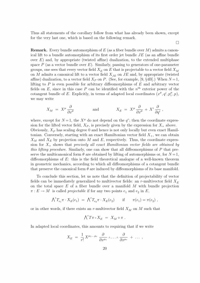
Thus all statements of the corollary follow from what has already been shown, exceptfor the very last one, which is based on the following remark.
Remark. Every bundle automorphism of E (as a fiber bundle over M) admits a canon-ical lift to a bundle automorphism of its first order jet bundle JE (as an affine bundleover E) and, by appropriate (twisted affine) dualization, to the extended multiphasespace P (as a vector bundle over E). Similarly, passing to generators of one-parametergroups, one sees that every vector field XE on E that is projectable to a vector field XM
on M admits a canonical lift to a vector field XJE on JE and, by appropriate (twistedaffine) dualization, to a vector field XP on P . (See, for example, [9, §4B].) When N =1,lifting to P is even possible for arbitrary diffeomorphisms of E and arbitrary vectorfields on E, since in this case P can be identified with the nth exterior power of thecotangent bundle of E. Explicitly, in terms of adapted local coordinates (xµ, qi, pµ
i , p),we may write
XM = Xµ ∂
∂xµ and XE = Xµ ∂
∂xµ + X i ∂
∂qi,
where, except for N =1, the Xµ do not depend on the qr; then the coordinate expres-sion for the lifted vector field, XP , is precisely given by the expression for X+ above.Obviously, XP has scaling degree 0 and hence is not only locally but even exact Hamil-tonian. Conversely, starting with an exact Hamiltonian vector field X+, we can obtainXM and XE by projection onto M and E, respectively. Thus, the coordinate expres-sion for X+ shows that precisely all exact Hamiltonian vector fields are obtained bythis lifting procedure. Similarly, one can show that all diffeomorphisms of P that pre-serve the multicanonical form θ are obtained by lifting of automorphisms or, for N =1,diffeomorphisms of E: this is the field theoretical analogue of a well-known theoremin geometric mechanics, according to which all diffeomorphisms of a cotangent bundlethat preserve the canonical form θ are induced by diffeomorphisms of its base manifold.
To conclude this section, let us note that the definition of projectability of vectorfields can be immediately generalized to multivector fields: an r-multivector field XE
on the total space E of a fiber bundle over a manifold M with bundle projectionπ : E → M is called projectable if for any two points e1 and e2 in E,∧r
Te1π ·XE(e1) =
∧rTe2
π ·XE(e2) if π(e1) = π(e2) ,
or in other words, if there exists an r-multivector field XM on M such that∧rTπ XE = XM π .
In adapted local coordinates, this amounts to requiring that if we write
XE =1
r!Xµ1... µr
∂
∂xµ1∧ . . . ∧
∂
∂xµr+ . . . ,
20
where the dots denote 1-vertical terms, the coefficients Xµ1... µr should depend only onthe local coordinates xρ for M but not on the local fiber coordinates qr for E. Now weintroduce the following terminology.
Definition 2.7 An r-multivector field on P is called projectable if it is projectablewith respect to any one of the three projections from P : to P0, to E and to M .
With this terminology, Theorem 2.4 states that for 0 < r < n, locally Hamiltonianr-multivector fields on P are projectable as soon as N >1 and are projectable to E butnot necessarily to P0 or to M when N =1. (Inspection of eq. (32) shows, however, thatthey are projectable to P0 if and only if they are projectable to M .)
Considering the special case of vector fields (r = 1), we believe that vector fieldson the total space of a fiber bundle over space-time which are not projectable shouldbe regarded as pathological, since they generate transformations which do not inducetransformations of space-time. It is hard to see how such transformations might beinterpreted as candidates for symmetries of a physical system. By analogy, we shalladopt the same point of view regarding multivector fields of higher degree, since al-though these do not generate diffeomorphisms of E as a manifold, they may perhapsallow for an interpretation as generators of superdiffeomorphisms of an appropriatesupermanifold built over E as its even part.
3 Poisson forms and Hamiltonian forms
Our aim in this section is to give an explicit construction of Poisson (n − r)-formsand, more generally, of Hamiltonian (n−r)-forms on the extended multiphase space P ,where 0 6 r 6 n. (Note that eq. (11) only makes sense for r in this range.) A specialrole is played by closed forms, since closed forms are always Hamiltonian and closedforms that vanish on the kernel of ω are always Poisson: these are in a sense the trivialexamples. In other words, the main task is to understand the extent to which generalHamiltonian forms deviate from closed forms and general Poisson forms deviate fromclosed forms that vanish on the kernel of ω.
As a warm-up exercise, we shall settle the extreme cases of tensor degree 0 and n.The case r = n has already been analyzed in Ref. [3], so we just quote the result.
Proposition 3.1 A function f on P , regarded as a 0-form, is always Hamiltonianand even Poisson. Moreover, its associated Hamiltonian n-multivector field X is, inadapted local coordinates and modulo terms taking values in the kernel of ω, given byeq. (29).
The case r = 0 is equally easy.
21
Proposition 3.2 An n-form f on P is Hamiltonian or Poisson if and only if it canbe written as the sum of a constant multiple of θ with a closed form which is arbitraryif f is Hamiltonian and vanishes on the kernel of ω if f is Poisson.
Indeed, if f is a Hamiltonian n-form, the multivector field X that appears in eq. (11) willin fact be a function which has to be locally Hamiltonian and hence, by Proposition 2.2,constant. Thus df must be proportional to ω and so f must be the sum of some constantmultiple of θ and a closed form.
The intermediate cases (0 < r < n) are much more interesting. To handle them,the first step is to identify the content of the kernel condition (13) in adapted localcoordinates (for completeness, we also include the two extreme cases):
Proposition 3.3 An (n− r)-form f on P , with 0 6 r 6 n, vanishes on the kernelof ω if and only if, in adapted local coordinates, it can be written in the form
f = 1r!
fµ1... µr dnxµ1... µr+ 1
(r+1)!fµ0... µr
i dqi ∧ dnxµ0... µr+ 1
r!f i,µ1... µr dpµ
i ∧ dnxµµ1... µr
+ 1(r+1)!
f ′µ0... µr
(dp ∧ dnxµ0... µr
− dqi ∧ dpµi ∧ dnxµ0... µrµ
),
(46)
where the second term in the last bracket is to be omitted if r = n−1 whereas only thefirst term remains if r = n.
Note that for one-forms (just as for functions), the kernel condition (13) is void, sinceω is non-degenerate. Also, it is in this case usually more convenient to replace eq. (46)by the standard local coordinate representation
f = fµ dxµ + fi dqi + f iµ dpµ
i + f0 dp . (47)
Proof. From the particular expression for ω in adapted coordinates, we see first ofall that forms of degree n−r vanishing on the kernel of ω must be (n−r−2)-horizontal(since they vanish on 3-vertical multivector fields) and that the only term which is not(n−r−1)-horizontal is
dqi ∧ dpκk ∧ dnxµ0... µrµ .
Furthermore, f has to vanish on the bivectors
∂
∂qi∧
∂
∂pκk
+ δki
∂
∂p∧
∂
∂xκand
∂
∂pµi
∧∂
∂xν +∂
∂pνi
∧∂
∂xµ
which yields the statement of the proposition.
The proposition above can be used to prove the following interesting and useful fact.
22

Proposition 3.4 An (n− r)-form f on P , with 0 6 r 6 n, vanishes on the kernelof ω if and only if there exists an (r + 1)-multivector field X on P such that
f = iXω . (48)
Then obviously,df = LXω . (49)
In particular, f is closed if and only if X is locally Hamiltonian.
At every point P , the statement that the inclusion of the kernel of ω in the kernelof f implies that there is a multivector Y such that iY ω = f at this point, can beshown without reference to the particular form of ω [1]. However, the expression for ωin adapted coordinates shows that we can even obtain a multivector field Y with thisproperty.Proof. The “if” part being obvious, observe that it suffices to prove the “only if”part locally, in the domain of definition of an arbitrary system of adapted local coordi-nates, by constructing the coefficients of X from those of f . (Indeed, since the relationbetween f and X postulated in eq. (48) is purely algebraic, i.e., it does not involvederivatives, we can construct a global solution patching together local solutions witha partition of unity.) A comparison of iXω, where X is an (r + 1)-multivector field [!]given by eq. (26), with (46) shows that when r < n, this can be achieved by setting
Xµ0... µr = (−1)r f ′µ0... µr , X i,µ1... µr = (−1)r f i,µ1... µr , (50)
Xµ0... µr
i = (−1)r+1 fµ0... µr
i , Xµ1... µr= − fµ1... µr , (51)
while for r = n, only the last equation is pertinent (for r = n− 1, the same conclusioncan also be reached by comparing (28) and (47)).
Corollary 3.5 An (n − r)-form f on P , with 0 6 r 6 n, is a Hamiltonian form ifand only if df vanishes on the kernel of ω and is a Poisson form if and only if both dfand f vanish on the kernel of ω.
With these preliminaries out of the way, we can proceed to the construction ofPoisson forms which are not closed. As we shall see, there are two such constructionswhich, taken together, will be sufficient to handle the general case.
The first construction is a generalization of the universal multimomentum map ofRef. [3], which to each exact Hamiltonian r-multivector field F on P associates a Poisson(n−r)-form J(F ) on P defined by eq. (52) below. What remained unnoticed in Ref. [3]is that this construction works even when X is only locally Hamiltonian. In fact, wehave the following generalization of Proposition 4.3 of Ref. [3]:
23
Proposition 3.6 For every locally Hamiltonian r-multivector field F on P , with0 6 r 6 n, the formula
J(F ) = (−1)r−1 iF θ (52)
defines a Poisson (n − r)-form J(F ) on P whose associated Hamiltonian multivectorfield is F + [Σ, F ], that is, we have
d (J(F )) = iF+[Σ,F ]ω . (53)
Proof. Obviously, J(F ) vanishes on the kernel of ω since this is contained in the kernelof θ. Moreover, since LF ω is supposed to vanish, we can use the algebraic relations forthe Lie derivative along multivector fields and θ = −iΣω to compute
d (J(F )) = (−1)r−1 d (iF θ) = (−1)r−1 LF θ − iF dθ
= (−1)r LF iΣω + iΣLF ω + iF ω = − i[F,Σ]ω + iF ω .
The second construction uses differential forms on E, pulled back to differentialforms on P via the target projection τ : P → E. Characterizing which of these areHamiltonian forms and which are Poisson forms is a simple exercise.
Proposition 3.7 Let f0 be an (n− r)-form on E, with 0 < r < n. Then
• τ ∗f0 is a Hamiltonian form on P if and only if df0 is (n− r)-horizontal.
• τ ∗f0 is a Poisson form on P if and only if f0 is (n− r− 1)-horizontal and df0 is(n− r)-horizontal.
Proof. In adapted local coordinates (xµ, qi) for E and (xµ, qi, p µi , p ) for P , we can
write
f0 =1
r!fµ1... µr
0 dnxµ1... µr+
1
(r+1)!(f0)
µ0... µr
i dqi ∧ dnxµ0... µr+ . . . , (54)
where the dots denote higher order terms containing at least two dq’s. Now applyingProposition 3.3 to τ ∗f0, we see that τ ∗f0 will vanish on the kernel of ω if and only theterms denoted by the dots all vanish, i.e., if f0 can be written in the form
f0 =1
r!fµ1... µr
0 dnxµ1... µr+
1
(r+1)!(f0)
µ0... µr
i dqi ∧ dnxµ0... µr. (55)
But this is precisely the condition for the (n− r)-form f0 to be (n− r − 1)-horizontal.(Note that this equivalence holds even when r = n − 1, provided we understand thecondition of being 0-horizontal to be empty.) Similarly, since Proposition 3.4 impliesthat a form on P is Hamiltonian if and only if its exterior derivative vanishes on the
24
kernel of ω, the same argument applied to d(τ ∗f0) = τ ∗df0 shows that, irrespectivelyof whether τ ∗f0 itself vanishes on the kernel of ω or not and hence whether we useeq. (54) or eq. (55) as our starting point, τ ∗f0 will be Hamiltonian if and only if
df0 = 1(r−1)!
∂fµ2... µrν0
∂xνdnxµ2... µr
+ 1r!
(∂fµ1... µr
0
∂qi− ∂(f0)
µ1... µrνi
∂xν
)dqi ∧ dnxµ1... µr
.
But this is precisely the condition for the (n− r + 1)-form df0 to be (n− r)-horizontal.Moreover, it is easy to write down an associated Hamiltonian r-multivector field X0:
X0 = (−1)r
r!
(∂fµ1... µr
0
∂qi− ∂(f0)
µ1... µrνi
∂xν
)∂
∂pµ1
i
∧∂
∂xµ2∧ . . . ∧
∂
∂xµr
− 1(r−1)!
∂fµ2... µrν0
∂xν
∂
∂p∧
∂
∂xµ2∧ . . . ∧
∂
∂xµr.
Note also that if f0 is (n− r − 1)-horizontal and thus has the form stated in eq. (55),df0 would contain just one additional higher order term, namely
1
(r+1)!
∂(f0)µ0... µr
j
∂qidqi ∧ dqj ∧ dnxµ0... µr
.
Its absence means that∂(f0)
µ0... µr
j
∂qi=
∂(f0)µ0... µr
i
∂qj,
so there exist local functions fµ0... µr
0 on E such that
(f0)µ0... µr
i =∂fµ0... µr
0
∂qi.
This implies that f0 can be written as the sum
f0 = fh + fc (56)
of a horizontal form fh and a closed form fc, defined by setting
fh =1
r!
(fµ1... µr
0 − ∂fµ1... µrν0
∂xν
)dnxµ1... µr
,
and
fc =1
r!
∂fµ1... µrν0
∂xνdnxµ1... µr
+1
(r+1)!
∂fµ0... µr
0
∂qidqi ∧ dnxµ0... µr
.
The same kind of local decomposition into the sum of a horizontal form and a closedform can also be derived if f0 is arbitrary and thus has the form stated in eq. (54);this case can be handled by decreasing induction on the number of dq’s that appear in
25
the higher order terms denoted by the dots in eq. (54). We shall refrain from workingthis out in detail, since unfortunately the decomposition (56) depends on the system ofadapted local coordinates used in its construction: under coordinate transformations,the terms fh and fc mix. Therefore, this decomposition has no coordinate independentmeaning and is in general valid only locally.
Finally, we note that in the above discussion, we have deliberately excluded theextreme cases r = 0 (n-forms) and r = n (functions). For n-forms, the equivalencesstated above would be incorrect since if f0 has tensor degree n and hence X0 has tensordegree 0, iX0
ω would by Proposition 2.2 be a constant multiple of ω whereas d(τ ∗f0)would be reduced to a linear combination of terms of the form dqi ∧ dnx, implyingthat τ ∗f0 can only be Hamiltonian if it is closed. For functions, the construction isuninteresting since according to Proposition 3.1, all functions on P are Poisson, andnot just the ones lifted from E.
Now we are ready to state our main decomposition theorem. (In what follows, weshall simply write f0 instead of τ ∗f0 when there is no danger of confusion, the mainexception being the proof of Theorem 3.8 below).
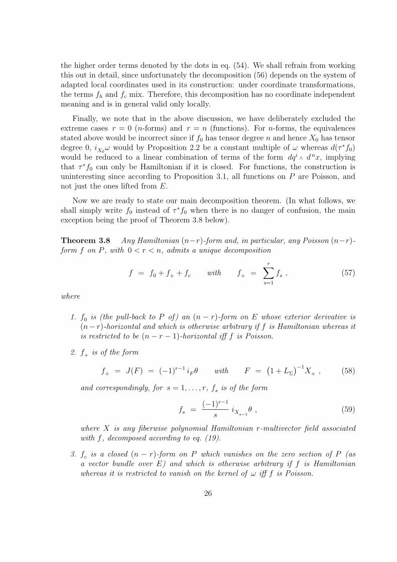
Theorem 3.8 Any Hamiltonian (n−r)-form and, in particular, any Poisson (n−r)-form f on P , with 0 < r < n, admits a unique decomposition
f = f0 + f+ + fc with f+ =r∑
s=1
fs , (57)
where
1. f0 is (the pull-back to P of) an (n − r)-form on E whose exterior derivative is(n− r)-horizontal and which is otherwise arbitrary if f is Hamiltonian whereas itis restricted to be (n− r − 1)-horizontal iff f is Poisson.
2. f+ is of the form
f+ = J(F ) = (−1)r−1 iF θ with F =(1 + LΣ
)−1X+ , (58)
and correspondingly, for s = 1, . . . , r, fs is of the form
fs =(−1)r−1
siXs−1
θ , (59)
where X is any fiberwise polynomial Hamiltonian r-multivector field associatedwith f , decomposed according to eq. (19).
3. fc is a closed (n − r)-form on P which vanishes on the zero section of P (asa vector bundle over E) and which is otherwise arbitrary if f is Hamiltonianwhereas it is restricted to vanish on the kernel of ω iff f is Poisson.
26

We shall refer to eq. (57) and to eq. (60) below as the canonical decomposition ofHamiltonian forms or Poisson forms on P .
Proof. Let f be a Poisson (n − r)-form and X be a Hamiltonian r-multivector fieldassociated with f . As already mentioned in the introduction, we may without loss ofgenerality assume X to be fiberwise polynomial and decompose it into homogeneouscomponents with respect to scaling degree, according to eq. (19):
X = X− + X+ + ξ with X+ =r∑
s=1
Xs−1 .
Then defining F as in the theorem, or equivalently, by
F =r∑
s=1
Fs−1 with Fs−1 =1
sXs−1 ,
we obtainF + [Σ, F ] = X+,
and hence according to eq. (53), the exterior derivative of the difference f − J(F ) isgiven by
d(f − J(F )
)= df − d
(J(F )
)= iXω − iX+
ω = iX−ω .
Applying the equivalence stated in eq. (23), we see that since X− has scaling degree −1,iX−ω must have scaling degree 0 and hence, according to Proposition A.1, is the pull-
back to P of some (n− r)-form f ′0 on E:
d(f − J(F )
)= iX−ω = τ ∗f ′
0 .
Next, we define f0 to be the restriction of f − J(F ) to the zero section of P , or moreprecisely, its pull-back to E with the zero section s0 : E → P ,
f0 = s∗0(f − J(F )
),
and setfc = f − τ ∗f0 − J(F ) .
Then
dfc = d(f − J(F )
)− d
(τ ∗s∗0
(f − J(F )
))= d(f − J(F )
)− τ ∗s∗0 d
(f − J(F )
)= τ ∗f ′
0 − τ ∗s∗0 τ ∗f ′0 = 0 ,
ands∗0fc = s∗0
(f − J(F )
)− s∗0 τ ∗f0 = f0 − s∗0 τ ∗f0 = 0 ,
27

showing that indeed, fc is closed and vanishes on the zero section of P .
Proof of Theorem 1.3, item 2. These statements are immediate consequences ofTheorem 3.8.
Remark. It should be noted that despite appearances, the decompositions (57) ofTheorem 3.8 and (21) of Theorem 1.3 are not necessarily identical: for s = 1, . . . , r, thefs of eq. (57) and the fs of eq. (21) may differ by homogeneous closed (n − r)-formsof scaling degree s. But the decomposition (57) of Theorem 3.8 seems to be the morenatural one.
Theorem 3.8 implies that Poisson forms have a rather intricate local coordinate re-presentation, involving two locally Hamiltonian multivector fields. Indeed, if we take fto be a general Poisson (n−r)-form on P , with 0 < r < n, we can apply Propositions 3.4and 3.6 to rewrite eq. (57) in the form
f = f0 + (−1)r−1iF θ + (−1)riFcω , (60)
where f0 is as before while F and Fc are two locally Hamiltonian multivector fieldson P of tensor degree r and r + 1, respectively, satisfying F− = 0 and (Fc)− = 0.4
In terms of the standard local coordinate representations (46) for f , (55) for f0, (26)for F and for Fc, and for θ and ω, eqs (2 and (3, we obtain
fµ1... µr = (−1)r−1 p F µ1... µr +r∑
s=1
(−1)r−s pµs
i Fi,µ1... µs−1µs+1... µr
+ fµ1... µr
0 + (−1)r−1(Fc)µ1... µr , (61)
fµ0... µr
i = −r∑
s=0
(−1)s pµs
i Fµ0... µs−1µs+1... µr + (f0)
µ0... µr
i − (Fc)µ0... µr
i , (62)
f i,µ1... µr = (Fc)i,µ1... µr , (63)
f ′µ0... µr = (Fc)µ0... µr , (64)
where the coefficients of F and of Fc are subject to the constraints listed in Theorem 2.4;in particular, the coefficients (Fc)
µ0... µr
i and (Fc)µ1... µr can be completely expressed in
terms of the coefficients (Fc)µ0... µr and (Fc)
i,µ1... µr , according to eqs (32) and (33) (withr replaced by r + 1, X replaced by Fc and X− replaced by 0). In particular, we seethat the coefficients fµ1... µr are “antisymmetric polynomials in the multimomentumvariables” of degree r. More explicitly, we can rewrite eq. (61) in the form
fµ1... µr = (−1)r−1 p F µ1... µr +r∑
s=1
fµ1... µrs + fµ1... µr
0 + (−1)r−1(Fc)µ1... µr ,
4The condition (Fc)− = 0 will guarantee that iFcω vanishes on the zero section of P .
28
where inserting the expansion (31) (with X replaced by F , Xs−1 replaced by Fs−1 andYs−1 replaced by Gs−1 = 1
sgs) gives, after a short calculation,
fµ1... µrs = (−1)r−1 1
s!
1
(r−s)!
∑π ∈Sr
(−1)π pµπ(1)
i1. . . p
µπ(s)
isg
i1... is,µπ(s+1)... µπ(r)s .
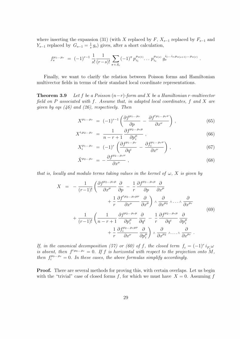
Finally, we want to clarify the relation between Poisson forms and Hamiltonianmultivector fields in terms of their standard local coordinate representations.
Theorem 3.9 Let f be a Poisson (n−r)-form and X be a Hamiltonian r-multivectorfield on P associated with f . Assume that, in adapted local coordinates, f and X aregiven by eqs (46) and (26), respectively. Then
Xµ1... µr = (−1)r−1
(∂fµ1... µr
∂p− ∂f ′µ1... µrν
∂xν
), (65)
X i,µ2... µr =1
n− r + 1
∂fµ2... µrµ
∂pµi
, (66)
Xµ1... µr
i = (−1)r
(∂fµ1... µr
∂qi− ∂fµ1... µrν
i
∂xν
), (67)
Xµ2... µr = − ∂fµ2... µrν
∂xν, (68)
that is, locally and modulo terms taking values in the kernel of ω, X is given by
X = − 1
(r−1)!
(∂fµ2... µrµ
∂xµ
∂
∂p− 1
r
∂fµ2... µrµ
∂p
∂
∂xµ
+1
r
∂f ′µ2... µrµν
∂xν
∂
∂xµ
)∧
∂
∂xµ2∧ . . . ∧
∂
∂xµr
+1
(r−1)!
(1
n− r + 1
∂fµ2... µrµ
∂pµi
∂
∂qi− 1
r
∂fµ2... µrµ
∂qi
∂
∂pµi
+1
r
∂fµ2... µrµνi
∂xν
∂
∂pµi
)∧
∂
∂xµ2∧ . . . ∧
∂
∂xµr.
(69)
If, in the canonical decomposition (57) or (60) of f , the closed term fc = (−1)r iFcω
is absent, then f ′µ0... µr = 0. If f is horizontal with respect to the projection onto M ,then fµ0... µr
i = 0. In these cases, the above formulas simplify accordingly.
Proof. There are several methods for proving this, with certain overlaps. Let us beginwith the “trivial” case of closed forms f , for which we must have X = 0. Assuming f
29
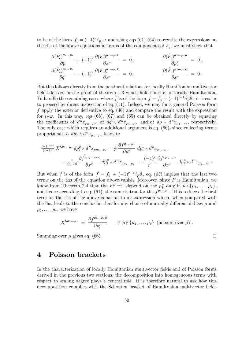
to be of the form fc = (−1)r iFcω and using eqs (61)-(64) to rewrite the expressions on
the rhs of the above equations in terms of the components of Fc, we must show that
∂(Fc)µ1... µr
∂p+ (−1)r ∂(Fc)
µ1... µrν
∂xν= 0 ,
∂(Fc)µ2... µrµ
∂pµi
= 0 ,
∂(Fc)µ1... µr
∂qi− (−1)r ∂(Fc)
µ1... µrνi
∂xν= 0 ,
∂(Fc)µ2... µrν
∂xν= 0 .
But this follows directly from the pertinent relations for locally Hamiltonian multivectorfields derived in the proof of theorem 1.3 which hold since Fc is locally Hamiltonian.To handle the remaining cases where f is of the form f = f0 + (−1)r−1 iF θ , it is easierto proceed by direct inspection of eq. (11). Indeed, we may for a general Poisson formf apply the exterior derivative to eq. (46) and compare the result with the expressionfor iXω. In this way, eqs (68), (67) and (65) can be obtained directly by equatingthe coefficients of dnxµ2... µr , of dqi ∧ dnxµ1... µr and of dp ∧ dnxµ1... µr , respectively.The only case which requires an additional argument is eq. (66), since collecting termsproportional to dpµ
i ∧ dnxµ1... µr leads to
(−1)r−1
(r−1)!X i,µ2... µr dpµ
i ∧ dnxµµ2... µr = 1r!
∂fµ1... µr
∂pµi
dpµi ∧ dnxµ1... µr
− 1(r−1)!
∂f i,µ2... µrν
∂xνdpµ
i ∧ dnxµµ2... µr− (−1)r
r!
∂f i,µ1... µr
∂xµdpµ
i ∧ dnxµ1... µr.
But when f is of the form f = f0 + (−1)r−1 iF θ , eq. (63) implies that the last twoterms on the rhs of the equation above vanish. Moreover, since F is Hamiltonian, weknow from Theorem 2.4 that the F µ1... µr depend on the pµ
i only if µ ∈ µ1, . . . , µr,and hence according to eq. (61), the same is true for the fµ1... µr . This reduces the firstterm on the rhs of the above equation to an expression which, when compared withthe lhs, leads to the conclusion that for any choice of mutually different indices µ andµ2, . . . , µr, we have
X i,µ2... µr =∂fµ2... µrµ
∂pµi
if µ /∈ µ2, . . . , µr (no sum over µ) .
Summing over µ gives eq. (66).
4 Poisson brackets
In the characterization of locally Hamiltonian multivector fields and of Poisson formsderived in the previous two sections, the decomposition into homogeneous terms withrespect to scaling degree plays a central role. It is therefore natural to ask how thisdecomposition complies with the Schouten bracket of Hamiltonian multivector fields
30
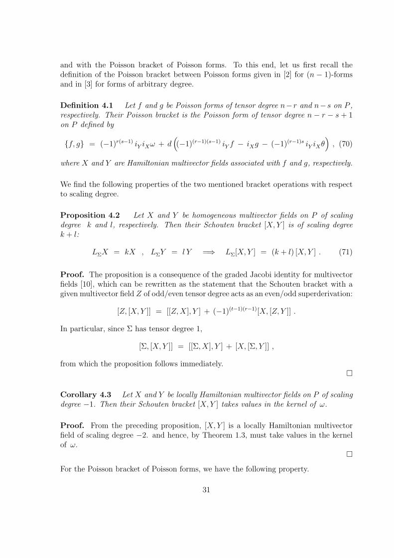
and with the Poisson bracket of Poisson forms. To this end, let us first recall thedefinition of the Poisson bracket between Poisson forms given in [2] for (n − 1)-formsand in [3] for forms of arbitrary degree.
Definition 4.1 Let f and g be Poisson forms of tensor degree n− r and n−s on P ,respectively. Their Poisson bracket is the Poisson form of tensor degree n − r − s + 1on P defined by
f, g = (−1)r(s−1) iY iXω + d((−1)(r−1)(s−1) iY f − iXg − (−1)(r−1)s iY iXθ
), (70)
where X and Y are Hamiltonian multivector fields associated with f and g, respectively.
We find the following properties of the two mentioned bracket operations with respectto scaling degree.
Proposition 4.2 Let X and Y be homogeneous multivector fields on P of scalingdegree k and l, respectively. Then their Schouten bracket [X, Y ] is of scaling degreek + l:
LΣX = kX , LΣY = l Y =⇒ LΣ[X,Y ] = (k + l) [X, Y ] . (71)
Proof. The proposition is a consequence of the graded Jacobi identity for multivectorfields [10], which can be rewritten as the statement that the Schouten bracket with agiven multivector field Z of odd/even tensor degree acts as an even/odd superderivation:
[Z, [X, Y ]] = [[Z,X], Y ] + (−1)(t−1)(r−1)[X, [Z, Y ]] .
In particular, since Σ has tensor degree 1,
[Σ, [X, Y ]] = [[Σ, X], Y ] + [X, [Σ, Y ]] ,
from which the proposition follows immediately.
Corollary 4.3 Let X and Y be locally Hamiltonian multivector fields on P of scalingdegree −1. Then their Schouten bracket [X,Y ] takes values in the kernel of ω.
Proof. From the preceding proposition, [X, Y ] is a locally Hamiltonian multivectorfield of scaling degree −2. and hence, by Theorem 1.3, must take values in the kernelof ω.
For the Poisson bracket of Poisson forms, we have the following property.
31
Proposition 4.4 Let f and g be homogeneous Poisson forms on P of scaling degree kand l, respectively. Then their Poisson bracket f, g is of scaling degree k + l − 1:
LΣf = kf , LΣg = l g =⇒ LΣf, g = (k + l − 1) f, g . (72)
Proof. As explained in the last paragraph of Section 1 (see, in particular, eq. (23)),we can find homogeneous Hamiltonian multivector fields X of scaling degree k− 1 andY of scaling degree l − 1 such that iXω = df and iY ω = dg . We shall consider eachof the terms in the definition of the Poisson bracket separately. We find
LΣ (iY iXω) = iY LΣiXω + i[Σ,Y ]iXω = iY iXLΣω + iY i[Σ,X]ω + i[Σ,Y ]iXω
= (k + l − 1) iY iXω .
The same calculation works with ω replaced by θ, so that, since LΣ commutes with d,
LΣ (d (iY iXθ)) = (k + l − 1) d (iY iXθ) .
Moreover,
LΣ (d (iY f))= d (LΣiY f) = d(iY LΣf + i[Σ,Y ]f
)= (k + l − 1) d (iY f) ,
and similarly LΣ (d (iXg)) = (k + l − 1) d (iXg). Putting the pieces together, theproposition follows.
Having shown in what sense both the Schouten bracket and the Poisson bracket re-spect scaling degree, let us use the canonical decomposition of Poisson forms to expresstheir Poisson bracket in terms of known operations on the simpler objects from whichthey can be constructed. To start with, we settle the case of homogeneous Poissonforms of positive scaling degree.
Proposition 4.5 Let Xk−1 be a homogeneous locally Hamiltonian r-multivector fieldon P of scaling degree k−1 and Yl−1 be a homogeneous locally Hamiltonian s-multivectorfield on P of scaling degree l − 1, with 1 6 k, l 6 r. Set
fk =(−1)r−1
kiXk−1
θ , gl =(−1)s−1
liYl−1
θ .
Then
fk, gl =(−1)r+s
k + l − 1i[Yl−1,Xk−1]θ − (−1)(r−1)s (k − 1)(l − 1)(k + l)
kl(k + l − 1)d(iXk−1
iYl−1θ)
.
Proof. From the defining equation (70) for the Poisson bracket, we find
fk, gl = (−1)r(s−1) iYl−1iXk−1
ω
+ d((−1)(r−1)s
kiYl−1
iXk−1θ − (−1)(s−1)
liXk−1
iYl−1θ
− (−1)(r−1)s iYl−1iXk−1
θ)
= (−1)r(s−1) iYl−1iXk−1
ω + (−1)(r−1)s(1
k+
1
l− 1)
d(iYl−1
iXk−1θ)
.
32
On the other hand, one verifies that diXk−1θ = k(−1)r−1iXk−1
ω and hence
i[Yl−1,Xk−1] θ = (−1)(s−1)rLYl−1iXk−1
θ − iXk−1LYl−1
θ
= (−1)(s−1)r d iYl−1iXk−1
θ + (−1)s(r−1)(k + l − 1) iYl−1iXk−1
ω .
Thus,
fk, gl =(−1)r+s
k + l − 1i[Yl−1,Xk−1]θ −
(−1)(r−1)s
k + l − 1d(iYl−1
iXk−1θ)
+ (−1)(r−1)s(1
k+
1
l− 1)
d(iYl−1
iXk−1θ)
, (73)
which implies the asserted relation.
As a special case, consider homogeneous Poisson forms of scaling degree 1, which ariseby contracting θ with a Hamiltonian multivector field of scaling degree 0, that is, with anexact Hamiltonian multivector field (see the first statement in Proposition 2.5). ThesePoisson forms have been studied in [3] under the name “universal multimomentummap”.
Corollary 4.6 The space of homogeneous Poisson forms on P of scaling degree 1closes under the Poisson bracket.
Obviously, it also follows from the proposition that no such statement holds for homo-geneous Poisson forms of scaling degree > 1, since the second term in the expression inProposition 4.5 vanishes only for k = 1 or l = 1.
Turning to homogeneous Poisson forms on P of scaling degree 0, which come fromforms on E by pull-back, we have
Proposition 4.7 The space of homogeneous Poisson forms on P of scaling degree 0is abelian under the Poisson bracket:
f0, g0 = 0 . (74)
Proof. Without loss of generality, we may assume the Hamiltonian multivector fieldsX− and Y− associated with f0 and with g0, respectively, to be homogeneous of scalingdegree −1. Therefore, using the fact that if a multivector field X is homogeneous ofscaling degree k and a differential form α is homogeneous of scaling degree l, then thedifferential form iXα is homogeneous of scaling degree k + l,
LΣX = kX , LΣα = lα =⇒ LΣ iXα = (k + l)iXα ,
which follows immediately from the formula LΣiXα = iXLΣα+ i[Σ,X]α , we see that all
four terms in the definition (70) of the Poisson bracket between f0 and g0 are differential
33
forms of scaling degree −1 and hence must vanish.
For the mixed case of the Poisson bracket between a homogeneous Poisson form ofstrictly positive scaling degree with one of scaling degree zero, we find the followingresult.
Proposition 4.8 Let Xk−1 be a homogeneous locally Hamiltonian r-multivector fieldon P of scaling degree k − 1, with 1 6 k 6 r, and let g0 be a homogeneous Poisson(n − s)-form on P of scaling degree zero, with associated Hamiltonian s-multivectorfield Y−. Set
fk =(−1)r−1
kiXk−1
θ . (75)
Thenfk, g0 = − LXk−1
g0 . (76)
Proof. By Proposition 2.5, iY−θ vanishes. Hence only two of the four terms in thedefining equation (70) for the Poisson bracket survive:
fk, g0 = (−1)r(s−1) iY−iXk−1ω − diXk−1
g0
= −(diXk−1
g0 − (−1)r iXk−1dg0
)= − LXk−1
g0 .
Finally, let us consider closed Poisson forms, whose associated Hamiltonian multi-vector fields vanish. Still, the Poisson bracket of a closed Poisson form with an arbitraryPoisson form does not vanish, but it is once again a closed Poisson form.
Proposition 4.9 Let f be a Poisson (n−r)-form on P , with associated Hamiltonianr-multivector field X, and let g be a closed Poisson (n− s)-form on P . Set
g = (−1)siGcω . (77)
Thenf, g = (−1)r+s−1i[Gc,X]ω . (78)
Proof. As the Hamiltonian multivector field associated with g vanishes, only one ofthe four terms in the defining equation (70) for the Poisson bracket survives:
f, g = − d (iXg) = (−1)s−1 d(iXiGc
ω)
= (−1)rs−1i[X,Gc]ω = (−1)r+s−1i[Gc,X]ω .
(For the penultimate equation, see, e.g., Proposition 3.3 of Ref. [3].)
In view of the canonical decomposition for Poisson forms stated in Theorem 3.8, theabove propositions exhaust the possible combinations for the computation of Poissonbrackets.
34
5 Conclusions and Outlook
In this paper, we have achieved three goals. First, we have determined the generalstructure of locally Hamiltonian multivector fields on the extended multiphase spaceof classical first order field theories. According to Theorem 2.4, the basic structurethat arises from explicit calculations in adapted local coordinates is the decompositionof any such multivector field X, of tensor degree r (0 < r < n), into a sum of termsof homogeneous scaling degree plus a remainder ξ which is a multivector field takingvalues in the kernel of ω:
X = X−1 + X0 + . . . + Xr−1 + ξ with LΣXk = kXk . (79)
Moreover, according to Proposition 2.5, all homogeneous locally Hamiltonian multi-vector fields of nonnegative scaling degree are in fact globally Hamiltonian, and theyare exact Hamiltonian if and only if they have zero scaling degree. At the level of localcoefficient functions, this decomposition arises because the coefficient functions have tobe antisymmetric polynomials in the multimomentum variables; see eqs (30) and (31).
Second, we have extended the scaling degree analysis to the study of Hamiltonianforms by means of the formula
LΣiXω = iX+[Σ,X]ω .
As shown in Theorem 3.8, this leads to a canonical decomposition of any Hamiltonian(n − r)-form f (0 < r < n) into a sum of terms of homogeneous scaling degree plus aremainder fc which is a closed form:
f = f0 + f1 + . . . + fr + fc with LΣfs = sfs . (80)
Moreover, if X is a Hamiltonian multivector field associated with f , then
fs =(−1)r−1
siXs−1
θ for s > 0 , (81)
where the Xs−1 are the homogeneous components of X of nonnegative scaling degree asdescribed before, whereas f0 arises by pull-back from a form on the total space of theconfiguration bundle of the theory. Locally, this form can be decomposed into the sumof a horizontal form and a closed form (we prove this explicitly only for Poisson forms),but this decomposition has no global, coordinate invariant meaning. The canonicaldecomposition of Poisson forms is also useful for deriving local formulas for X in termsof f ; these are given in Theorem 3.9. They clearly show that the situation in multi-symplectic geometry resembles that encountered in symplectic geometry but exhibits asignificantly richer structure. In particular, the notion of conjugate variables requiresa conceptual extension.
Third, we have used the canonical decomposition of Poisson forms to derive explicitformulas for the Poisson bracket between Poisson forms. The resulting Lie algebra shows
35
an interesting and nontrivial structure. It has a trivial part, namely the space of closedPoisson forms, which constitutes an ideal that one might wish to divide out: this ideal isabelian but not central. It commutes with the most interesting and useful part, namelythe subalgebra of homogeneous Poisson forms of scaling degree 1, which by means ofeq. (81), specialized to the case s=1, correspond to the exact Hamiltonian multivectorfields, and in such a way that the Poisson bracket on this subalgebra corresponds to theSchouten bracket for exact Hamiltonian multivector fields (up to signs). The nontrivialmixing occurs through the spaces of homogeneous Poisson forms of scaling degree 0and of scaling degree > 1: they close under the operation of taking the Poisson bracketwith a homogeneous Poisson forms of scaling degree 1 but not under the operation oftaking mutual Poisson brackets, since these contain contributions lying in the ideal ofclosed Poisson forms.
An important aspect of our results is that they confirm, once again, the apparentlyunavoidable appearance of strong constraints on the dependence of Hamiltonian multi-vector fields and Hamiltonian forms on the multimomentum variables and the energyvariable in extended multiphase space, expressed through the “antisymmetric poly-nomial” structure of their coefficient functions. This strongly suggests that there shouldbe some product structure complementing the Poisson bracket operation. So far, sucha structure seems to exist only for a very restricted class of Poisson forms, namelythe horizontal forms studied by Kanatchikov [11]. Also, one might wonder whetherthe structural properties derived here still hold in the multisymplectic formulation ofhigher order field theories [8].
Finally, a central question that remains is how the various proposals of Poissonbrackets in the multisymplectic formalism that can be found in the literature, includ-ing the one proposed in Refs [2] and [3], relates to the Peierls - DeWitt bracket thatcomes from the functional approach based on the concept of covariant phase space.Briefly, covariant phase space is defined as the space S of solutions of the equationsof motion and, formally viewed as an infinite-dimensional manifold, carries a naturallydefined symplectic form Ω [14–16]. A systematic general investigation of the Peierls -DeWitt bracket in the multisymplectic framework, including a proof of the fact that itis precisely the canonical Poisson bracket for functionals on S derived from the sym-plectic form Ω on S, has been carried out recently [12, 13]. In order to establish thedesired relation, we must restrict this bracket to a certain class of functionals, namelyfunctionals F obtained by using fields to pull Hamiltonian forms or Poisson forms f onextended multiphase space back to space-time and then integrate over submanifolds Σof the corresponding dimension. Explicitly, using the notation of Ref. [13], we have
F [φ] =
∫Σ
(FL (ϕ, ∂ϕ)
)∗f (82)
in the Lagrangian framework and
F [φ] =
∫Σ
(H (ϕ, π)
)∗f (83)
36
in the Hamiltonian framework. Now using the classification of Hamiltonian vectorfields and Hamiltonian (n−1)-forms obtained in this paper, it has been shown recentlythat the Peierls -DeWitt bracket F, G between two functionals F and G derived fromHamiltonian (n − 1)-forms f and g, respectively, is the functional derived from theHamiltonian (n − 1)-form f, g [17]; details will be published elsewhere. The ques-tion of how to extend this result to Poisson forms of other degree is currently underinvestigation.
6 Acknowledgements
Part of this work has been financially supported by CNPq (“Conselho Nacionalde Desenvolvimento Cientıfico e Tecnologico”), Brazil (M.F.), by DFG (“DeutscheForschungsgemeinschaft”), Germany, under the Emmy Noether Programme (C.P.), andby FAPESP (“Fundao de Amparo a Pesquisa do Estado de Sao Paulo”, Brazil (H.R.).
A Appendix
Proposition A.1 Let V be a vector bundle over a manifold M with projection π andlet Σ be the scaling or Euler vector field on V . A differential form α on the total space Vwill be the pull-back of a differential form α0 on the base space M to V via π if andonly if it is scale invariant:
α = π∗α0 ⇐⇒ LΣα = 0 .
Proof. Assume first that the form α on V is the pull-back of a form α0 on M ; thenα = π∗α0 and hence dα = π∗dα0. Therefore, α and dα are both horizontal. Thismeans that for any vertical vector field X on V , including Σ, we have iXα = 0 as wellas iXdα = 0, so LXα = 0.Conversely, assume that the form α on V , of degree r, say, satisfies LΣα = 0, so α isinvariant under the flow F of Σ [4]:
d
dλF ∗
λα = 0 .
This means that given v ∈V and w1, . . . , wr ∈ TvV , the expression
(F ∗λα)v(w1, . . . , wr) = αFλ(v)(TvFλ · w1 , . . . , TvFλ · wr)
does not depend on λ, so its value αv(w1, . . . , wr) at λ = 0 is equal to its valueαv0
((w1)0, . . . , (wr)0) obtained in the limit λ → −∞, where v0 denotes the zero vectorin the fiber of v. But this means that α is equal to π∗α0 where α0 is defined with thehelp of the zero section i0 : M → V of V as α0 = i∗0α.
The following lemma is used in the proof of Theorem 2.4:
37
Lemma A.2 Let f be a polynomial of degree s in a set of variables xµ. Let fr, 0 ≤r ≤ s, be the homogeneous component of degree r of f . Then
f =s∑
r=1
1
rxµ ∂fr
∂xµ+ f0 .
Proof. For the operator xµ ∂∂xµ , the homogeneous polynomials fr are eigenvectors with
eigenvalue r. Writing this as fr = 1rxµ ∂fr
∂xµ for 0 < r ≤ s, we obtain
f =s∑
r=0
fr = f0 +s∑
r=1
1
rxµ ∂fr
∂xµ.
References
[1] R. Bryant, private communication (2005).
[2] M. Forger & H. Romer: A Poisson Bracket on Multisymplectic Phase Space,Rep. Math. Phys. 48 (2001) 211-218; math-ph/0009037.
[3] M. Forger, C. Paufler & H. Romer: The Poisson Bracket for PoissonForms in Multisymplectic Field Theory, Rev. Math. Phys. 15 (2003) 705-744;math-ph/0202043.
[4] For the sake of brevity, we have left out straightforward but tedious parts of theproofs. The reader may find more detailed guidelines in the arXiv version of thisarticle under math-ph/0407057v1.
[5] J. Kijowski: A Finite-dimensional Canonical Formalism in the Classical FieldTheory, Commun. Math. Phys. 30 (1973) 99-128.
[6] J. Kijowski & W. Szczyrba: Multisymplectic Manifolds and the GeometricalConstruction of the Poisson Brackets in the Classical Field Theory, in: J.-M.Souriau (ed.): Geometrie Symplectique et Physique Mathematique, pp. 347-379,C.N.R.S., Paris 1975.
[7] J.F. Carinena, M. Crampin & L.A. Ibort: On the Multisymplectic Formal-ism for First Order Field Theories, Diff. Geom. Appl. 1 (1991) 345-374.
[8] M.J. Gotay: A Multisymplectic Framework for Classical Field Theory and theCalculus of Variations I: Covariant Hamiltonian formalism, in: M. Francaviglia &D.D. Holm (eds): Mechanics, Analysis and Geometry: 200 years after Lagrange,pp. 203-235, 1991.
38
[9] M.J. Gotay, J. Isenberg & J.E. Marsden: Momentum Maps and ClassicalRelativistic Fields I: Covariant Field Theory, physics/9801019.
[10] W.M. Tulczyew: The Graded Lie Algebra of Multivector Fields and the Gener-alized Lie Derivative of Forms, Bull. Acad. Pol. Sci., Ser. Sci. Math. Astron. Phys.22 (1974) 937-942.
[11] I.V. Kanatchikov: On Field Theoretic Generalizations of a Poisson Algebra,Rep. Math. Phys. 40 (1997) 225-234, hep-th/9710069.
[12] S.V. Romero: Colchete de Poisson Covariante na Teoria Geometrica dos Cam-pos, PhD thesis, IME-USP, June 2001.
[13] M. Forger & S.V. Romero: Covariant Poisson Brackets in Geometric FieldTheory, Preprint IME-USP RT-MAP-0304, to appear in Commun. Math. Phys.
[14] C. Crnkovic & E. Witten: Covariant Description of Canonical Formalism inGeometrical Theories, in: W. Israel & S. Hawking (eds): Three Hundred Years ofGravitation, pp. 676-684, Cambridge 1987.
[15] C. Crnkovic: Symplectic Geometry of Covariant Phase Space, Class. QuantumGrav. 5 (1988) 1557-1575.
[16] G. Zuckerman: Action Principles and Global Geometry, in: S.-T. Yau (ed.):Mathematical Aspects of String Theory, pp. 259-288, World Scientific, Singapore1987.
[17] M.O. Salles: Campos Hamiltonianos e Colchete de Poisson na Teoria Geo-metrica dos Campos, PhD thesis, IME-USP, June 2004.
39