Embed Size (px)
Citation preview
Hankel determinants, continued fractions,orthgonal polynomials,
and hypergeometric series
Ira M. Gesselwith Jiang Zeng and Guoce Xin
LaBRIJune 8, 2007
Continued fractions and Hankel determinants
There is a close relationship between continued fractions,Hankel determinants, and orthogonal polynomials.
Why are we interested in these things?
Continued fractions count certain “weighted Motzkin paths”which encode objects of enumerative interest such as partitionsand permutations. (Flajolet)
Hankel determinants arise in some enumeration problems, forexample, counting certain kinds of tilings or alternating signmatrices.
Orthogonal polynomials
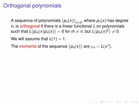
A sequence of polynomials(pn(x)
)n≥0, where pn(x) has degree
n, is orthogonal if there is a linear functional L on polynomialssuch that L
(pm(x)pn(x)
)= 0 for m 6= n, but L
(pm(x)2) 6= 0.
We will assume that L(1) = 1.
The moments of the sequence(pn(x)
)are µn = L(xn). So
µ0 = 1.
Theorem. The sequence(pn(x)
)of monic polynomials is
orthogonal if and only if there exist numbers(an)
n≥0 and(bn)
n≥1, with bn 6= 0 for all n ≥ 1 such that
xpn(x) = pn+1(x) + anpn(x) + bnpn−1(x), n ≥ 1
with p0(x) = 1 and p1(x) = x − a0.
Orthogonal polynomials
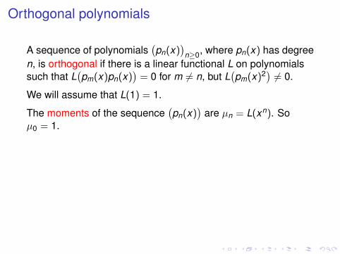
A sequence of polynomials(pn(x)
)n≥0, where pn(x) has degree
n, is orthogonal if there is a linear functional L on polynomialssuch that L
(pm(x)pn(x)
)= 0 for m 6= n, but L
(pm(x)2) 6= 0.
We will assume that L(1) = 1.
The moments of the sequence(pn(x)
)are µn = L(xn).
Soµ0 = 1.
Theorem. The sequence(pn(x)
)of monic polynomials is
orthogonal if and only if there exist numbers(an)
n≥0 and(bn)
n≥1, with bn 6= 0 for all n ≥ 1 such that
xpn(x) = pn+1(x) + anpn(x) + bnpn−1(x), n ≥ 1
with p0(x) = 1 and p1(x) = x − a0.
Orthogonal polynomials
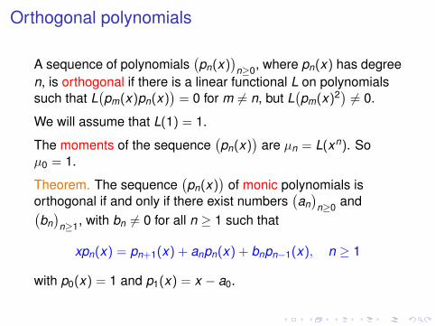
A sequence of polynomials(pn(x)
)n≥0, where pn(x) has degree
n, is orthogonal if there is a linear functional L on polynomialssuch that L
(pm(x)pn(x)
)= 0 for m 6= n, but L
(pm(x)2) 6= 0.
We will assume that L(1) = 1.
The moments of the sequence(pn(x)
)are µn = L(xn). So
µ0 = 1.
Theorem. The sequence(pn(x)
)of monic polynomials is
orthogonal if and only if there exist numbers(an)
n≥0 and(bn)
n≥1, with bn 6= 0 for all n ≥ 1 such that
xpn(x) = pn+1(x) + anpn(x) + bnpn−1(x), n ≥ 1
with p0(x) = 1 and p1(x) = x − a0.
Orthogonal polynomials
A sequence of polynomials(pn(x)
)n≥0, where pn(x) has degree
n, is orthogonal if there is a linear functional L on polynomialssuch that L
(pm(x)pn(x)
)= 0 for m 6= n, but L
(pm(x)2) 6= 0.
We will assume that L(1) = 1.
The moments of the sequence(pn(x)
)are µn = L(xn). So
µ0 = 1.
Theorem. The sequence(pn(x)
)of monic polynomials is
orthogonal if and only if there exist numbers(an)
n≥0 and(bn)
n≥1, with bn 6= 0 for all n ≥ 1 such that
xpn(x) = pn+1(x) + anpn(x) + bnpn−1(x), n ≥ 1
with p0(x) = 1 and p1(x) = x − a0.
The connection
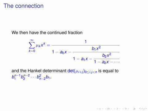
We then have the continued fraction∞∑
k=0
µkxk =1
1− a0x −b1x2
1− a1x −b2x2
1− a2x − · · ·
and the Hankel determinant det(µi+j)0≤i,j<n is equal tobn−1
1 bn−22 · · ·b2
n−2b1.
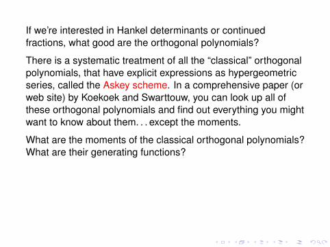
If we’re interested in Hankel determinants or continuedfractions, what good are the orthogonal polynomials?
There is a systematic treatment of all the “classical” orthogonalpolynomials, that have explicit expressions as hypergeometricseries, called the Askey scheme. In a comprehensive paper (orweb site) by Koekoek and Swarttouw, you can look up all ofthese orthogonal polynomials and find out everything you mightwant to know about them. . . except the moments.
What are the moments of the classical orthogonal polynomials?What are their generating functions?Why do some, but not all of them, have nice exponentialgenerating functions?
What are the orthogonal polynomials whose moments are theGenocchi numbers?
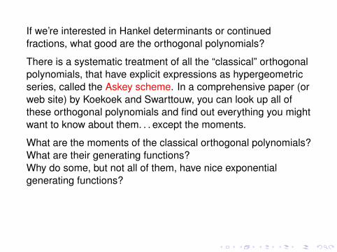
If we’re interested in Hankel determinants or continuedfractions, what good are the orthogonal polynomials?
There is a systematic treatment of all the “classical” orthogonalpolynomials, that have explicit expressions as hypergeometricseries, called the Askey scheme. In a comprehensive paper (orweb site) by Koekoek and Swarttouw, you can look up all ofthese orthogonal polynomials and find out everything you mightwant to know about them. . .
except the moments.
What are the moments of the classical orthogonal polynomials?What are their generating functions?Why do some, but not all of them, have nice exponentialgenerating functions?
What are the orthogonal polynomials whose moments are theGenocchi numbers?
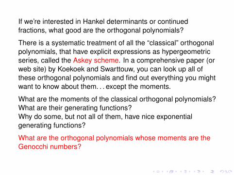
If we’re interested in Hankel determinants or continuedfractions, what good are the orthogonal polynomials?
There is a systematic treatment of all the “classical” orthogonalpolynomials, that have explicit expressions as hypergeometricseries, called the Askey scheme. In a comprehensive paper (orweb site) by Koekoek and Swarttouw, you can look up all ofthese orthogonal polynomials and find out everything you mightwant to know about them. . . except the moments.
What are the moments of the classical orthogonal polynomials?What are their generating functions?Why do some, but not all of them, have nice exponentialgenerating functions?
What are the orthogonal polynomials whose moments are theGenocchi numbers?
If we’re interested in Hankel determinants or continuedfractions, what good are the orthogonal polynomials?
There is a systematic treatment of all the “classical” orthogonalpolynomials, that have explicit expressions as hypergeometricseries, called the Askey scheme. In a comprehensive paper (orweb site) by Koekoek and Swarttouw, you can look up all ofthese orthogonal polynomials and find out everything you mightwant to know about them. . . except the moments.
What are the moments of the classical orthogonal polynomials?
What are their generating functions?Why do some, but not all of them, have nice exponentialgenerating functions?
What are the orthogonal polynomials whose moments are theGenocchi numbers?
If we’re interested in Hankel determinants or continuedfractions, what good are the orthogonal polynomials?
There is a systematic treatment of all the “classical” orthogonalpolynomials, that have explicit expressions as hypergeometricseries, called the Askey scheme. In a comprehensive paper (orweb site) by Koekoek and Swarttouw, you can look up all ofthese orthogonal polynomials and find out everything you mightwant to know about them. . . except the moments.
What are the moments of the classical orthogonal polynomials?What are their generating functions?
Why do some, but not all of them, have nice exponentialgenerating functions?
What are the orthogonal polynomials whose moments are theGenocchi numbers?
If we’re interested in Hankel determinants or continuedfractions, what good are the orthogonal polynomials?
There is a systematic treatment of all the “classical” orthogonalpolynomials, that have explicit expressions as hypergeometricseries, called the Askey scheme. In a comprehensive paper (orweb site) by Koekoek and Swarttouw, you can look up all ofthese orthogonal polynomials and find out everything you mightwant to know about them. . . except the moments.
What are the moments of the classical orthogonal polynomials?What are their generating functions?Why do some, but not all of them, have nice exponentialgenerating functions?
What are the orthogonal polynomials whose moments are theGenocchi numbers?
If we’re interested in Hankel determinants or continuedfractions, what good are the orthogonal polynomials?
There is a systematic treatment of all the “classical” orthogonalpolynomials, that have explicit expressions as hypergeometricseries, called the Askey scheme. In a comprehensive paper (orweb site) by Koekoek and Swarttouw, you can look up all ofthese orthogonal polynomials and find out everything you mightwant to know about them. . . except the moments.
What are the moments of the classical orthogonal polynomials?What are their generating functions?Why do some, but not all of them, have nice exponentialgenerating functions?
What are the orthogonal polynomials whose moments are theGenocchi numbers?
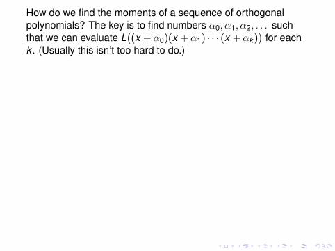
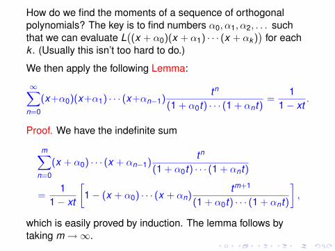
How do we find the moments of a sequence of orthogonalpolynomials? The key is to find numbers α0, α1, α2, . . . suchthat we can evaluate L
((x + α0)(x + α1) · · · (x + αk )
)for each
k . (Usually this isn’t too hard to do.)
We then apply the following Lemma:
∞∑n=0
(x+α0)(x+α1) · · · (x+αn−1)tn
(1 + α0t) · · · (1 + αnt)=
11− xt
.
Proof. We have the indefinite sum
m∑n=0
(x + α0) · · · (x + αn−1)tn
(1 + α0t) · · · (1 + αnt)
=1
1− xt
[1− (x + α0) · · · (x + αn)
tm+1
(1 + α0t) · · · (1 + αnt)
],
which is easily proved by induction. The lemma follows bytaking m →∞.
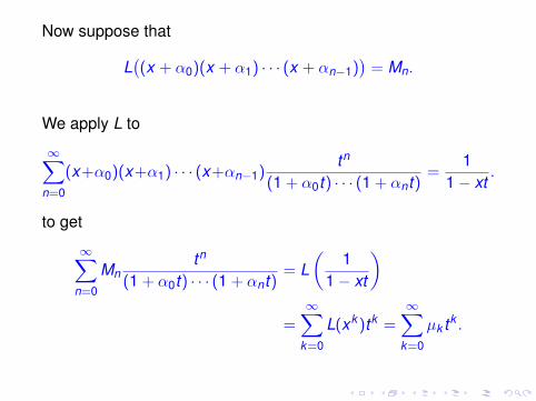
Now suppose that
L((x + α0)(x + α1) · · · (x + αn−1)
)= Mn.
We apply L to
∞∑n=0
(x+α0)(x+α1) · · · (x+αn−1)tn
(1 + α0t) · · · (1 + αnt)=
11− xt
.
to get
∞∑n=0
Mntn
(1 + α0t) · · · (1 + αnt)= L
(1
1− xt
)
=∞∑
k=0
L(xk )tk =∞∑
k=0
µk tk .
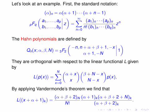
Let’s look at an example. First, the standard notation:
(α)n = α(α + 1) · · · (α + n − 1)
pFq
(a1, . . . , ap
b1, . . . , bp
∣∣∣∣ z) =∞∑
n=0
(a1)n · · · (ap)n
n! (b1)n · · · (bq)nzn
The Hahn polynomials are defined by
Qn(x ;α, β, N) = 3F2
(−n, n + α + β + 1,−x
α + 1,−N
∣∣∣∣ 1)They are orthogonal with respect to the linear functional L givenby
L(p(x)
)=
N∑x=0
(α + x
x
)(β + N − x
N − x
)p(x),
By applying Vandermonde’s theorem we find that
L((x + α + 1)k
)=
(α + β + 2)N
N!
(α + 1)k (α + β + 2 + N)k
(α + β + 2)k.
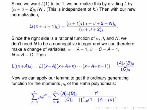
Since we want L(1) to be 1, we normalize this by dividing L by(α + β + 2)N/N!. (This is independent of k .) Then with our newnormalization,
L((x + α + 1)k
)=
(α + 1)k (α + β + 2 + N)k
(α + β + 2)k.
Since the right side is a rational function of α, β, and N, wedon’t need N to be a nonnegative integer and we can thereforemake a change of variables, α = A− 1, β = C − A− 1,N = B − C. Then
L((x +A)n
)= L
((x +A)(x +A+n) · · · (x +A+n−1)
)=
(A)n(B)n
(C)n.
Now we can apply our lemma to get the ordinary generatingfunction for the moments µn of the Hahn polynomials:
∞∑n=0
µntn =∞∑
n=0
(A)n(B)n
(C)n
tn∏nj=0(1 + (A + j)t)
.
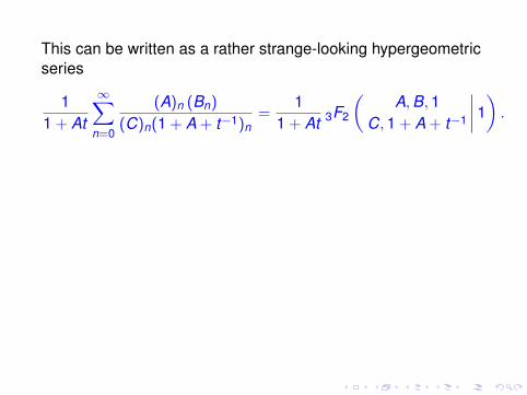
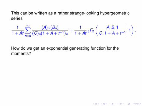
This can be written as a rather strange-looking hypergeometricseries
11 + At
∞∑n=0
(A)n (Bn)
(C)n(1 + A + t−1)n=
11 + At 3F2
(A, B, 1
C, 1 + A + t−1
∣∣∣∣ 1) .
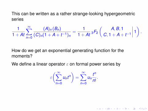
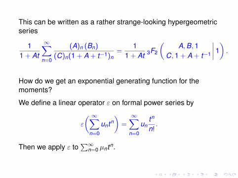
How do we get an exponential generating function for themoments?
We define a linear operator ε on formal power series by
ε
( ∞∑n=0
untn)
=∞∑
n=0
untn
n!.
Then we apply ε to∑∞
n=0 µntn.
This can be written as a rather strange-looking hypergeometricseries
11 + At
∞∑n=0
(A)n (Bn)
(C)n(1 + A + t−1)n=
11 + At 3F2
(A, B, 1
C, 1 + A + t−1
∣∣∣∣ 1) .
How do we get an exponential generating function for themoments?
We define a linear operator ε on formal power series by
ε
( ∞∑n=0
untn)
=∞∑
n=0
untn
n!.
Then we apply ε to∑∞
n=0 µntn.
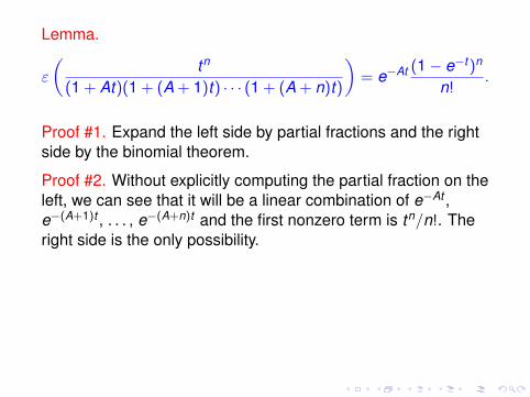
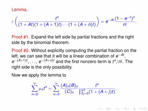
Lemma.
ε
(tn
(1 + At)(1 + (A + 1)t) · · · (1 + (A + n)t)
)= e−At (1− e−t)n
n!.
Proof #1. Expand the left side by partial fractions and the rightside by the binomial theorem.
Proof #2. Without explicitly computing the partial fraction on theleft, we can see that it will be a linear combination of e−At ,e−(A+1)t , . . . , e−(A+n)t and the first nonzero term is tn/n!. Theright side is the only possibility.
Now we apply the lemma to
∞∑n=0
µntn =∞∑
n=0
(A)n(B)n
(C)n
tn∏nj=0(1 + (A + j)t)
.
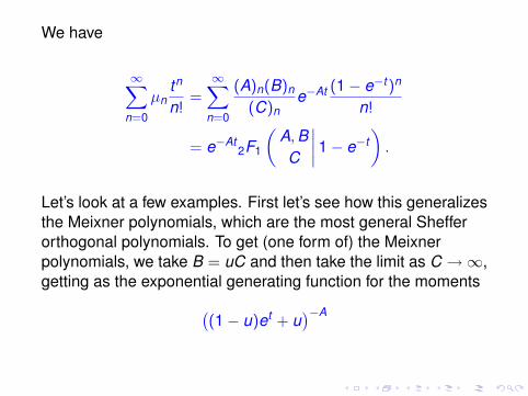
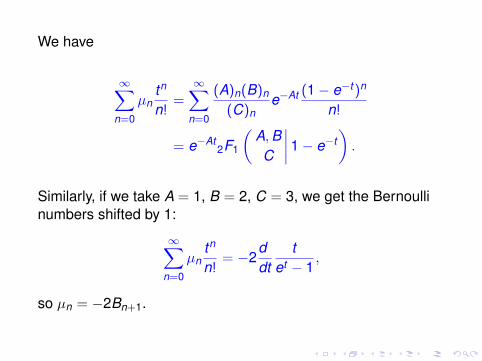
We have
∞∑n=0
µntn
n!=
∞∑n=0
(A)n(B)n
(C)ne−At (1− e−t)n
n!
= e−At2F1
(A, BC
∣∣∣∣ 1− e−t)
.
Let’s look at a few examples. First let’s see how this generalizesthe Meixner polynomials, which are the most general Shefferorthogonal polynomials. To get (one form of) the Meixnerpolynomials, we take B = uC and then take the limit as C →∞,getting as the exponential generating function for the moments(
(1− u)et + u)−A
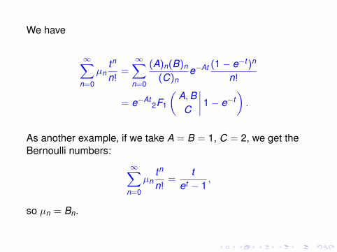
We have
∞∑n=0
µntn
n!=
∞∑n=0
(A)n(B)n
(C)ne−At (1− e−t)n
n!
= e−At2F1
(A, BC
∣∣∣∣ 1− e−t)
.
As another example, if we take A = B = 1, C = 2, we get theBernoulli numbers:
∞∑n=0
µntn
n!=
tet − 1
,
so µn = Bn.
We have
∞∑n=0
µntn
n!=
∞∑n=0
(A)n(B)n
(C)ne−At (1− e−t)n
n!
= e−At2F1
(A, BC
∣∣∣∣ 1− e−t)
.
Similarly, if we take A = 1, B = 2, C = 3, we get the Bernoullinumbers shifted by 1:
∞∑n=0
µntn
n!= −2
ddt
tet − 1
,
so µn = −2Bn+1.
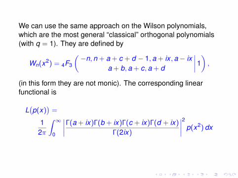
We can use the same approach on the Wilson polynomials,which are the most general “classical” orthogonal polynomials(with q = 1). They are defined by
Wn(x2) = 4F3
(−n, n + a + c + d − 1, a + ix , a− ix
a + b, a + c, a + d
∣∣∣∣ 1) ,
(in this form they are not monic). The corresponding linearfunctional is
L(p(x)
)=
12π
∫ ∞0
∣∣∣∣Γ(a + ix)Γ(b + ix)Γ(c + ix)Γ(d + ix)
Γ(2ix)
∣∣∣∣2 p(x2) dx
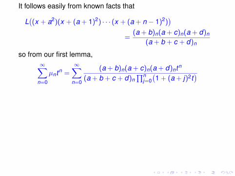
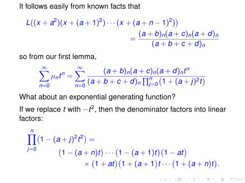
It follows easily from known facts that
L((x + a2)(x + (a + 1)2) · · · (x + (a + n − 1)2)
)=
(a + b)n(a + c)n(a + d)n
(a + b + c + d)n
so from our first lemma,∞∑
n=0
µntn =∞∑
n=0
(a + b)n(a + c)n(a + d)ntn
(a + b + c + d)n∏n
j=0(1 + (a + j)2t
)
What about an exponential generating function?
If we replace t with −t2, then the denominator factors into linearfactors:
n∏j=0
(1− (a + j)2t2) =(
1− (a + n)t)· · ·(1− (a + 1)t
)(1− at
)×(1 + at
)(1 + (a + 1
)t · · ·
(1 + (a + n)t
).
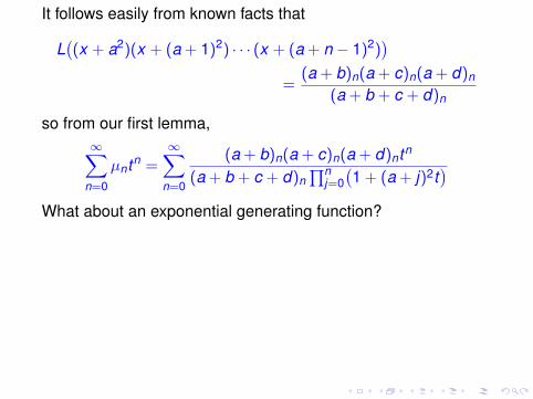
It follows easily from known facts that
L((x + a2)(x + (a + 1)2) · · · (x + (a + n − 1)2)
)=
(a + b)n(a + c)n(a + d)n
(a + b + c + d)n
so from our first lemma,∞∑
n=0
µntn =∞∑
n=0
(a + b)n(a + c)n(a + d)ntn
(a + b + c + d)n∏n
j=0(1 + (a + j)2t
)What about an exponential generating function?
If we replace t with −t2, then the denominator factors into linearfactors:
n∏j=0
(1− (a + j)2t2) =(
1− (a + n)t)· · ·(1− (a + 1)t
)(1− at
)×(1 + at
)(1 + (a + 1
)t · · ·
(1 + (a + n)t
).
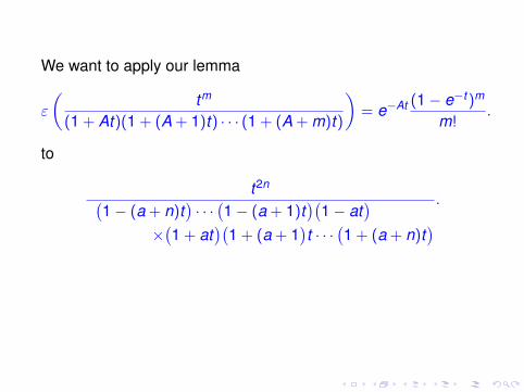
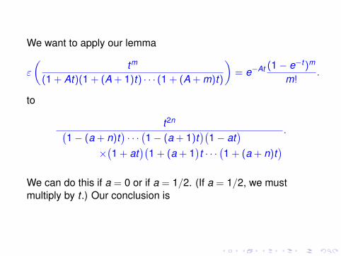
We want to apply our lemma
ε
(tm
(1 + At)(1 + (A + 1)t) · · · (1 + (A + m)t)
)= e−At (1− e−t)m
m!.
to
t2n(1− (a + n)t
)· · ·(1− (a + 1)t
)(1− at
)×(1 + at
)(1 + (a + 1
)t · · ·
(1 + (a + n)t
) .
We can do this if a = 0 or if a = 1/2. (If a = 1/2, we mustmultiply by t .) Our conclusion is
We want to apply our lemma
ε
(tm
(1 + At)(1 + (A + 1)t) · · · (1 + (A + m)t)
)= e−At (1− e−t)m
m!.
to
t2n(1− (a + n)t
)· · ·(1− (a + 1)t
)(1− at
)×(1 + at
)(1 + (a + 1
)t · · ·
(1 + (a + n)t
) .
We can do this if a = 0 or if a = 1/2. (If a = 1/2, we mustmultiply by t .) Our conclusion is
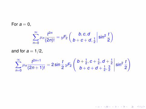
For a = 0,
∞∑n=0
µnt2n
(2n)!= 3F2
(b, c, d
b + c + d , 12
∣∣∣∣ sin2 t2
)and for a = 1/2,
∞∑n=0
µnt2n+1
(2n + 1)!= 2 sin
t2 3F2
(b + 1
2 , c + 12 , d + 1
2
b + c + d + 12 , 3
2
∣∣∣∣∣ sin2 t2
)
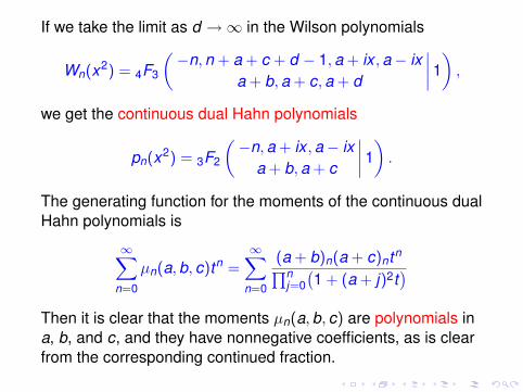
If we take the limit as d →∞ in the Wilson polynomials
Wn(x2) = 4F3
(−n, n + a + c + d − 1, a + ix , a− ix
a + b, a + c, a + d
∣∣∣∣ 1) ,
we get the continuous dual Hahn polynomials
pn(x2) = 3F2
(−n, a + ix , a− ix
a + b, a + c
∣∣∣∣ 1) .
The generating function for the moments of the continuous dualHahn polynomials is
∞∑n=0
µn(a, b, c)tn =∞∑
n=0
(a + b)n(a + c)ntn∏nj=0(1 + (a + j)2t
)Then it is clear that the moments µn(a, b, c) are polynomials ina, b, and c, and they have nonnegative coefficients, as is clearfrom the corresponding continued fraction.
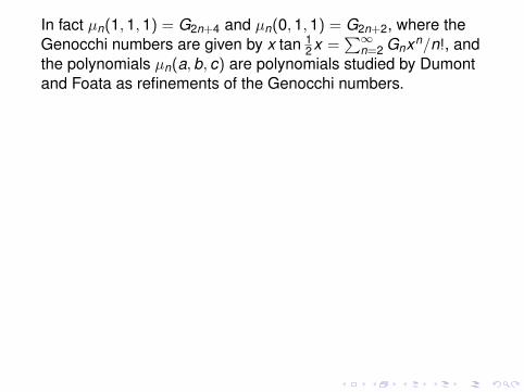
In fact µn(1, 1, 1) = G2n+4 and µn(0, 1, 1) = G2n+2, where theGenocchi numbers are given by x tan 1
2x =∑∞
n=2 Gnxn/n!, andthe polynomials µn(a, b, c) are polynomials studied by Dumontand Foata as refinements of the Genocchi numbers.
For a = 0 we have the generating function
∞∑n=0
µn(0, b, c)t2n
(2n)!= 2F1
(b, c
12
∣∣∣∣ sin2 t2
),
and it’s not hard to check that indeed,
2F1
(1, 1
12
∣∣∣∣ sin2 t2
)=
∞∑n=0
Gn+2xn
n!=
d2
dx2 x tanx2
using
2F1
(1, 1
12
∣∣∣∣ y2)
=
√1− y2 + y sin−1 y
(1− y2)3/2 .
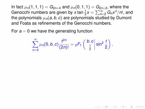
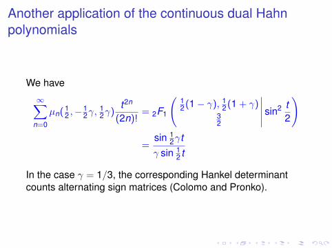
Another application of the continuous dual Hahnpolynomials
We have
∞∑n=0
µn(12 ,−1
2γ, 12γ)
t2n
(2n)!= 2F1
(12(1− γ), 1
2(1 + γ)32
∣∣∣∣∣ sin2 t2
)
=sin 1
2γtγ sin 1
2 t
In the case γ = 1/3, the corresponding Hankel determinantcounts alternating sign matrices (Colomo and Pronko).
Hankel Determinants and Ternary Tree Numbers
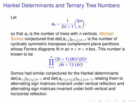
Let
an =1
2n + 1
(3nn
),
so that an is the number of trees with n vertices. MichaelSomos conjectured that det(ai+j)0≤i,j≤n−1 is the number ofcyclically symmetric transpose complement plane partitionswhose Ferrers diagrams fit in an n × n × n box. This number isknown to be
n∏i=1
(3i + 1) (6i)! (2i)!(4i + 1)! (4i)!
.
Somos had similar conjectures for the Hankel determinantsdet(ai+j)0≤i,j≤n−1 and det(a(i+j+1)/2)0≤i,j≤n−1, relating them toalternating sign matrices invariant under vertical reflection andalternating sign matrices invariant under both vertical andhorizontal reflection.
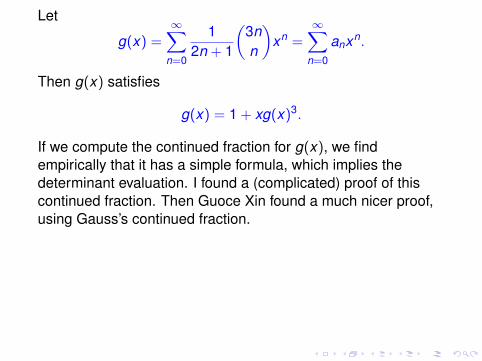
Let
g(x) =∞∑
n=0
12n + 1
(3nn
)xn =
∞∑n=0
anxn.
Then g(x) satisfies
g(x) = 1 + xg(x)3.
If we compute the continued fraction for g(x), we findempirically that it has a simple formula, which implies thedeterminant evaluation. I found a (complicated) proof of thiscontinued fraction. Then Guoce Xin found a much nicer proof,using Gauss’s continued fraction.
However, the same method had already been used by UlrichTamm to evaluate these determinants, before Somos stated hisconjectures.
(But there is no known combinatorial connection between theseHankel determinants and plane partitions or alternating signmatrices.)
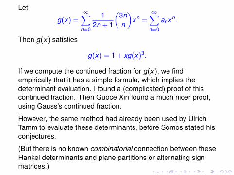
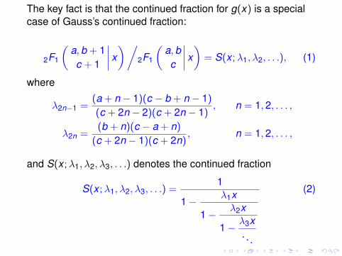
The key fact is that the continued fraction for g(x) is a specialcase of Gauss’s continued fraction:
2F1
(a, b + 1c + 1
∣∣∣∣ x)/2F1
(a, bc
∣∣∣∣ x) = S(x ;λ1, λ2, . . .), (1)
where
λ2n−1 =(a + n − 1)(c − b + n − 1)
(c + 2n − 2)(c + 2n − 1), n = 1, 2, . . . ,
λ2n =(b + n)(c − a + n)
(c + 2n − 1)(c + 2n), n = 1, 2, . . . ,
and S(x ;λ1, λ2, λ3, . . .) denotes the continued fraction
S(x ;λ1, λ2, λ3, . . .) =1
1− λ1x
1− λ2x
1− λ3x. . .
(2)
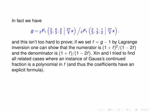
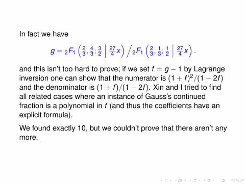
In fact we have
g = 2F1
(23 , 4
3 ; 32
∣∣∣ 274 x)/
2F1
(23 , 1
3 ; 12
∣∣∣ 274 x)
.
and this isn’t too hard to prove; if we set f = g − 1 by Lagrangeinversion one can show that the numerator is (1 + f )2/(1− 2f )and the denominator is (1 + f )/(1− 2f ). Xin and I tried to findall related cases where an instance of Gauss’s continuedfraction is a polynomial in f (and thus the coefficients have anexplicit formula).
We found exactly 10, but we couldn’t prove that there aren’t anymore.
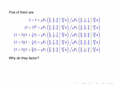
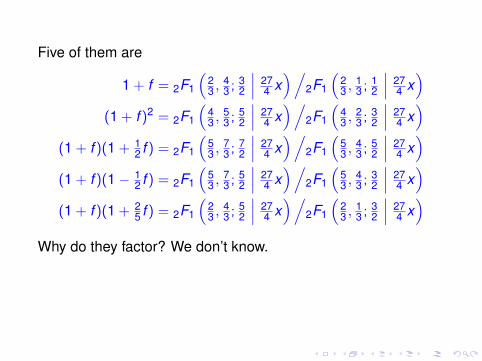
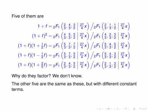
Five of them are
1 + f = 2F1
(23 , 4
3 ; 32
∣∣∣ 274 x)/
2F1
(23 , 1
3 ; 12
∣∣∣ 274 x)
(1 + f )2 = 2F1
(43 , 5
3 ; 52
∣∣∣ 274 x)/
2F1
(43 , 2
3 ; 32
∣∣∣ 274 x)
(1 + f )(1 + 12 f ) = 2F1
(53 , 7
3 ; 72
∣∣∣ 274 x)/
2F1
(53 , 4
3 ; 52
∣∣∣ 274 x)
(1 + f )(1− 12 f ) = 2F1
(53 , 7
3 ; 52
∣∣∣ 274 x)/
2F1
(53 , 4
3 ; 32
∣∣∣ 274 x)
(1 + f )(1 + 25 f ) = 2F1
(23 , 4
3 ; 52
∣∣∣ 274 x)/
2F1
(23 , 1
3 ; 32
∣∣∣ 274 x)
Why do they factor?
We don’t know.
The other five are the same as these, but with different constantterms.
Five of them are
1 + f = 2F1
(23 , 4
3 ; 32
∣∣∣ 274 x)/
2F1
(23 , 1
3 ; 12
∣∣∣ 274 x)
(1 + f )2 = 2F1
(43 , 5
3 ; 52
∣∣∣ 274 x)/
2F1
(43 , 2
3 ; 32
∣∣∣ 274 x)
(1 + f )(1 + 12 f ) = 2F1
(53 , 7
3 ; 72
∣∣∣ 274 x)/
2F1
(53 , 4
3 ; 52
∣∣∣ 274 x)
(1 + f )(1− 12 f ) = 2F1
(53 , 7
3 ; 52
∣∣∣ 274 x)/
2F1
(53 , 4
3 ; 32
∣∣∣ 274 x)
(1 + f )(1 + 25 f ) = 2F1
(23 , 4
3 ; 52
∣∣∣ 274 x)/
2F1
(23 , 1
3 ; 32
∣∣∣ 274 x)
Why do they factor? We don’t know.
The other five are the same as these, but with different constantterms.