Hash-based Subgraph Query Processing Method forGraph-structured XML Documents ∗

Hongzhi WangHarbin Institute of Tech.

wangzh@hit.edu.cn

Jianzhong LiHarbin Institute of Tech.

lijzh@hit.edu.cn

Jizhou LuoHarbin Institute of Tech.

luojizhou@hit.edu.cn

Hong GaoHarbin Institute of Tech.

honggao@hit.edu.cn

ABSTRACTWhen XML documents are modeled as graphs, many re-search issues arise. In particular, there are many new chal-lenges in query processing on graph-structured XML doc-uments because traditional query processing techniques fortree-structured XML documents cannot be directly applied.This paper studies the problem of structural queries on graph-structured XML documents. A hash-based structural joinalgorithm, HGJoin, is first proposed to handle reachabilityqueries on graph-structured XML documents. Then, it isextended to the algorithms to process structural queries inform of bipartite graphs. Finally, based on these algorithms,a strategy to process subgraph queries in form of generalDAGs is proposed. Analysis and experiments show that allthe algorithms have high performance. It is notable thatall the algorithms above can be slightly modified to processstructural queries in form of general graphs.

1. INTRODUCTIONXML has become the de facto standard for information

representation and exchange over the Internet. In manyapplications, an XML document needs to be modeled as agraph more naturally than a tree. For example, the XMLdocument of the relationship of publications and authorsadapts to graph structure since one paper may have morethan one author and one author may have more than onepaper. A fragment of such information is shown in Fig 1.Obviously, the graph-structured XML document can be rep-resented in tree structure by duplicating the element withmore than one incoming paths. But it will result in redun-dancy. If the information in Fig 1 is represented with atree-structured XML document, the element “author” will

∗Support by the Key Program of the National NaturalScience Foundation of China under Grant No.60533110;the National Grand Fundamental Research 973 Program ofChina under Grant No.2006CB303000; the National Natu-ral Science Foundation of China under Grant No.60773068and No.60773063

Permission to copy without fee all or part of this material is granted providedthat the copies are not made or distributed for direct commercial advantage,the VLDB copyright notice and the title of the publication and its date appear,and notice is given that copying is by permission of the Very Large DataBase Endowment. To copy otherwise, or to republish, to post on serversor to redistribute to lists, requires a fee and/or special permission from thepublisher, ACM.VLDB ‘08,August 24-30, 2008, Auckland, New ZealandCopyright 2008 VLDB Endowment, ACM 000-0-00000-000-0/00/00.

be duplicated.

b i b

p r o c e e d i n g s j o u r n a l s

p r o c e e d i n g

a r t i c l e

t i t l e

c o n f e r e n c e

j o u r n a l

I C D E

t 1

n a m e

T K D E

v o l u m e a r t i c l e

1 7 ( 2 ) t i t l e

t 2

a u t h o r

n a m e e m a i l

n 1 e 1

Figure 1: An Example of Graph-structured XML

Among the queries on graph-structured XML documents,the subgraph queries are widely used. A subgraph queryon graph-structured XML documents (subgraph query forshort) is to retrieve the subgraphs matching the graph inthe query. For instance, a subgraph query on the graph-structured XML document in Fig 1 is to retrieve the namesof authors with publications both in proceedings and jour-nals. Another subgraph query on the XML document inFig 1 is to retrieve the name of the journal with an authorwho published papers in the conference ICDE. Such queriesare difficult to represent with traditional tree-structured queries.

It is a big challenge to process subgraph queries efficiently.All the four kinds of traditional methods of processing struc-tural queries on tree-structured XML documents, structuraljoin based methods[2], holistic Twigjoin based methods[3],structural index based methods[14, 12] and subsequence match-ing based methods[23, 19], cannot be used to process sub-graph queries.

The structural join based methods and the holistic Twigjoinbased methods both depend on the labelling scheme spe-cially for tree-structured XML documents. The encodingscheme of the graph-structured XML documents is totallydifferent from that of the tree-structured XML documents.As a result, they cannot be used to process subgraph queries.

The structural index based methods of processing struc-tural queries on tree-structured XML documents requirethat the size of the index must be very small. However, theindices of the graph-structured XML documents are verylarge in general. Thus, the structural index based methods

478

Permission to make digital or hard copies of portions of this work for personal or classroom use is granted without fee provided that copies are not made or distributed for profit or commercial advantage and that copies bear this notice and the full citation on the first page. Copyright for components of this work owned by others than VLDB Endowment must be honored. Abstracting with credit is permitted. To copy otherwise, to republish, to post on servers or to redistribute to lists requires prior specific permission and/or a fee. Request permission to republish from: Publications Dept., ACM, Inc. Fax +1 (212) 869-0481 or permissions@acm.org. PVLDB '08, August 23-28, 2008, Auckland, New Zealand Copyright 2008 VLDB Endowment, ACM 978-1-60558-305-1/08/08

cannot be used to process the subgraph queries efficiently.The subsequence matching based methods require that

the tree-structured XML documents and the queries on thedocuments must be converted into sequences before queryprocessing. It is difficult to covert a graph-structured XMLdocument into a sequence so that it is not easy to pro-cess subgraph queries using the subsequence matching basedmethods.

A few methods has been proposed to process some kindsof subgraph queries on XML data in form of some specialkinds of graphs. A method, called StackD, is presented into [4] to process twig queries on DAG-structured data. It isa modification of a holistic TwigJoin based method. How-ever, StackD focuses on tree-structured twig queries and isnot suitable for queries in form of complex graphs. Addi-tionally, when there are many edges in the graph, StackDshould maintain a very large data structure. In this case,it needs very huge main memory space, which is not prac-tical and it becomes inefficient. Another modification ofthe holistic TwigJoin-based method is presented in [27] toprocess twig queries on graph-structured data. However, itonly works on a kind of special graphs, i.e. st-planar graphs[11], but not suitable for other graphs. In summary, currentmethods cannot process general subgraph queries effectivelyor efficiently.

To process general subgraph queries effectively and effi-ciently, a new method based on labeling scheme [17] is pro-posed in this paper. The reasons of choosing the labelingscheme [17] are as following.

• It contains only intervals and identifications (ids). Allintervals and ids are numerical values so that thereis an order on them, which makes query processingeasier.

• It is compatible with the adjacent labeling scheme sothat it can be used to process queries with both reach-ability and adjacent edges. We will discuss this indetails in Section 6.

• By slightly modification, the labeling scheme can beused to process graphs with circles.

Our proposed method is designed step by step. First,a hash-based join algorithm, HGJoin, is proposed for pro-cessing reachability queries on graph-structured XML. Sec-ond, the HGJoin algorithm is extended to the IT-HGJoinand T-HGJoin algorithms to process the reachability querieswith multiple ancestors or multiple descendants. Then, Bi-HGJoin, the combination of IT-HGJoin and T-HGJoin, isdesigned to process queries in form of complete bipartitegraphs. Finally, based on all the above algorithms, themethod for processing subgraph queries in form of DAGsis proposed.

Without losing generality, this paper will focus on sub-graph queries in form of DAG with only reachability rela-tionships on edges for the convenience of discussion. With aslight modification, the method can be used to process anygeneral subgraph queries.

The contributions of this paper are as follows:

• Based on the reachability scheme in [17], a family ofhash-based join algorithms is presented as basic oper-ators of subgraph query processing.

• For structural queries in form of general graphs, an ef-ficient method is presented. The basic idea is to splita query into bipartite subqueries each of which canbe processed by some HGJoin algorithm. In order tofind effective splitting strategy, a cost-based query op-timization strategy is presented with some accelerationstrategies .

• The extensive experimental results show that the pro-posed algorithms outperform the existing algorithmsand our query splitting strategy is effective and effi-cient.

The rest of this paper is organized as follows: Section 2introduces some background knowledge. Section 3 presentsthe basic version of HGJoin algorithm for reachability querywith one ancestor and one descendant. Section 4 illustratethe algorithms for queries in form of bipartite graphs. Thestrategy of processing queries in form of general DAGs isproposed in Section 5. The extensions of our method for thegeneral subgraph queries are discussed in Section 6. Experi-mental results and analysis are shown in Section 7. Relatedwork is discussed in Section 8 and Section 9 concludes thispaper.

2. PRELIMINARIESIn this section, the background and notations used in this

paper are presented.

2.1 Graph-structured XML Data and QueriesWith IDREF-ID in an XML document representing ref-

erence relationship, an XML document can be consideredas a tagged directed graph. Elements and attributes in anXML document is mapped to the nodes in a graph. Directednesting relationships and reference relationships in an XMLdocument is mapped to the edges in a graph. For exam-ple, an XML document is shown in Fig 2(a) and its graphstructure is shown in Fig 2(b).

In a graph-structured XML document, structural queriesare defined based on the structural relationship betweennodes. In the graph structure G of an XML document, twonodes a and b satisfy adjacent relationship if and only if anedge from a to b exists in G; two nodes a and b satisfy reach-ability relationship if and only if a path from a to b existsin G. A reachability query a → d is to retrieve all pairs ofnodes (na,nd) in G where na has tag a, nd has tag d and na

and nd satisfy reachabilty relationship in G. For example,the result of reachability a → e in the graph in Fig 2(b)includes (a,e1), (a, e2), (a,e3). Adjacent queries can be de-fined similarly. The combination of multiple reachability oradjacent relationships forms subgraph queries.

A subgraph query is a tagged directed graph Q={V , E,tag, rel}, where V is the node set of Q; E is the edge set of Q;the function tag : V → TAG is the tag function (TAG is theset of tags); the function rel : E → AXIS shows the struc-tural relationships between the nodes in the query (AXIS isthe set of relationships between nodes; PC ∈ AXIS repre-sents adjacent relationship; AD ∈ AXIS represents reacha-bility relationship). The directed graph (V ,E) is called thequery graph. If ab ∈ E and rel(ab) = PC, then ab is calledan adjacent edge. If ab ∈ E and rel(ab) = AD, then ab iscalled a reachability edge. In V , the nodes without incom-ing edges are called sources and the nodes without outgoing

479

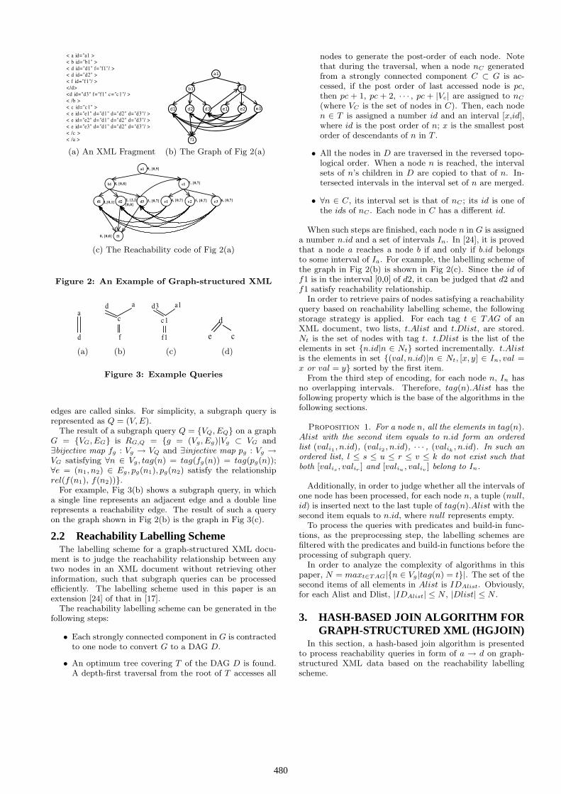
< a i d = " a 1 > < b i d = " b 1 " > < d i d = " d 1 " f = " f 1 " / > < d i d = " d 2 " > < f i d = " f 1 " / > < / d > < d i d = " d 3 " f = " f 1 " c = " c 1 " / > < / b > < c i d = " c 1 " > < e i d = " e 1 " d = " d 1 " d = " d 2 " d = " d 3 " / > < e i d = " e 2 " d = " d 1 " d = " d 2 " d = " d 3 " / > < e i d = " e 3 " d = " d 1 " d = " d 2 " d = " d 3 " / > < / c > < / a >

(a) An XML Fragment (b) The Graph of Fig 2(a)

a 1

b 1 c 1

d 1 d 2 d 3 e 1 e 2 e 3

f 1 0 , [ 0 , 0 ]

1 , [ 0 , 1 ] 2 , [ 2 , 2 ] [ 0 , 0 ]

3 , [ 0 , 7 ] 6 , [ 0 , 7 ] 5 , [ 0 , 7 ] 4 , [ 0 , 7 ]

7 , [ 0 , 7 ] 8 , [ 0 , 8 ]

9 , [ 0 , 9 ]

(c) The Reachability code of Fig 2(a)

Figure 2: An Example of Graph-structured XML

a

d

(a)

d a

c

f

(b)

d 3 a 1

c 1

f 1

(c)

d

e c

(d)

Figure 3: Example Queries

edges are called sinks. For simplicity, a subgraph query isrepresented as Q = (V, E).

The result of a subgraph query Q = {VQ, EQ} on a graphG = {VG, EG} is RG,Q = {g = (Vg, Eg)|Vg ⊂ VG and∃bijective map fg : Vg → VQ and ∃injective map pg : Vg →VG satisfying ∀n ∈ Vg, tag(n) = tag(fg(n)) = tag(pg(n));∀e = (n1, n2) ∈ Eg, pg(n1), pg(n2) satisfy the relationshiprel(f(n1), f(n2))}.

For example, Fig 3(b) shows a subgraph query, in whicha single line represents an adjacent edge and a double linerepresents a reachability edge. The result of such a queryon the graph shown in Fig 2(b) is the graph in Fig 3(c).

2.2 Reachability Labelling SchemeThe labelling scheme for a graph-structured XML docu-

ment is to judge the reachability relationship between anytwo nodes in an XML document without retrieving otherinformation, such that subgraph queries can be processedefficiently. The labelling scheme used in this paper is anextension [24] of that in [17].

The reachability labelling scheme can be generated in thefollowing steps:

• Each strongly connected component in G is contractedto one node to convert G to a DAG D.

• An optimum tree covering T of the DAG D is found.A depth-first traversal from the root of T accesses all

nodes to generate the post-order of each node. Notethat during the traversal, when a node nC generatedfrom a strongly connected component C ⊂ G is ac-cessed, if the post order of last accessed node is pc,then pc + 1, pc + 2, · · · , pc + |Vc| are assigned to nC

(where VC is the set of nodes in C). Then, each noden ∈ T is assigned a number id and an interval [x,id],where id is the post order of n; x is the smallest postorder of descendants of n in T .

• All the nodes in D are traversed in the reversed topo-logical order. When a node n is reached, the intervalsets of n’s children in D are copied to that of n. In-tersected intervals in the interval set of n are merged.

• ∀n ∈ C, its interval set is that of nC ; its id is one ofthe ids of nC . Each node in C has a different id.

When such steps are finished, each node n in G is assigneda number n.id and a set of intervals In. In [24], it is provedthat a node a reaches a node b if and only if b.id belongsto some interval of Ia. For example, the labelling scheme ofthe graph in Fig 2(b) is shown in Fig 2(c). Since the id off1 is in the interval [0,0] of d2, it can be judged that d2 andf1 satisfy reachability relationship.

In order to retrieve pairs of nodes satisfying a reachabilityquery based on reachability labelling scheme, the followingstorage strategy is applied. For each tag t ∈ TAG of anXML document, two lists, t.Alist and t.Dlist, are stored.Nt is the set of nodes with tag t. t.Dlist is the list of theelements in set {n.id|n ∈ Nt} sorted incrementally. t.Alistis the elements in set {(val, n.id)|n ∈ Nt, [x, y] ∈ In, val =x or val = y} sorted by the first item.

From the third step of encoding, for each node n, In hasno overlapping intervals. Therefore, tag(n).Alist has thefollowing property which is the base of the algorithms in thefollowing sections.

Proposition 1. For a node n, all the elements in tag(n).Alist with the second item equals to n.id form an orderedlist (vali1 , n.id), (vali2 , n.id), · · · , (valik , n.id). In such anordered list, l ≤ s ≤ u ≤ r ≤ v ≤ k do not exist such thatboth [valis , valir ] and [valiu , valiv ] belong to In.

Additionally, in order to judge whether all the intervals ofone node has been processed, for each node n, a tuple (null,id) is inserted next to the last tuple of tag(n).Alist with thesecond item equals to n.id, where null represents empty.

To process the queries with predicates and build-in func-tions, as the preprocessing step, the labelling schemes arefiltered with the predicates and build-in functions before theprocessing of subgraph query.

In order to analyze the complexity of algorithms in thispaper, N = maxt∈TAG|{n ∈ Vg|tag(n) = t}|. The set of thesecond items of all elements in Alist is IDAlist. Obviously,for each Alist and Dlist, |IDAlist| ≤ N , |Dlist| ≤ N .

3. HASH-BASED JOIN ALGORITHM FORGRAPH-STRUCTURED XML (HGJOIN)

In this section, a hash-based join algorithm is presentedto process reachability queries in form of a → d on graph-structured XML data based on the reachability labellingscheme.

480

Algorithm 1 HGJoin

a=Alist.begind=Dlist.beginwhile a 6= Alist.end AND d 6= Dlist.end do

if vala ≤ idd thenif ida /∈ H then

H.insert(ida)a = a.nextNode

else if vala < idd thenH.delete(ida)a = a.nextNode

elsefor ∀id ∈ H do

append (id, idd) to OutputListd=d.nextNode;

elsefor ∀id ∈ H do

append (id, idd) to OutputListd=d.nextNode;

a a 1 1

a 2 2 a 2 3

( a 1 2 )

b ( b 1 1 )

c ( c 2 1 )

c 1 1 ( c 1 2 )

b 1 2

( b 2 1 )

d

( c 3 2 )

c 1 3

( d 1 1 ) d 1 2

( d 2 1 )

e e 1 e 2

( d 3 1 )

e 3

c 2 2

( a 2 1 )

( b 3 1 )

( a 3 1 )

( b 4 1 )

a 3 2

c 3 1

( a 4 1 )

( b 5 1 )

Figure 4: Example data

Based on the storage strategy, suppose Alist = tag(a).Alistand Dlist = tag(d).Dlist. Intuitively, for any idj ∈ Dlist, iftwo tuples in Alist, (x, idi) and (y,idi), satisfy x ≤ idi ≤ yand [x, y] is an interval of the labelling scheme of some node,then (idi, idj) belongs to the result set. Proposition 1 as-sures that the query can be processed with scanning Alistand Dlist alternately only once. During the scan, a hashtable H is used to store ids of nodes satisfying the conditionthat for each node n, the start point x of some interval inIn has been scanned while corresponding end point y is notmet. Proportion 1 shows that before such y is met, none ofthe start points of other intervals in In will be met. When acorresponding y is met, n.id will be removed from H. Thestep is shown as following. At first, cursors a and d are as-signed to Alist and Dlist, respectively. During the scan ofAlist, if the current tuple (vala,ida) satisfies vala ≤ idd andida ∈ H, it means that the end position of some interval ismet and such an interval is impossible to contain idd. Sincethe elements in Dlist is in incremental order, and such aninterval is impossible to contain other unscanned elementsin Dlist. So ida is removed from H and a is updated. Ifvala = ida and ida ∈ H or vala > idd, it means that idd iscontained in some interval with vala as the end point. Insuch an instance, partial results are outputted and the scanis switched to Dlist. During the scan of Dlist, if idd < vala,or vala = ida and ida ∈ H, then based on the propertiesof elements in H, for ∀id ∈ H, (id, idd) is outputted andd is updated; if idd > vala, or vala = idd but ida /∈ H, itmeans that vala is possibly the start position of an inter-val containing idd and the scan is switched to Alist. Thepseudo-code of HGJoin is shown in Algorithm 1.

b c d

e

(a)

b c d

a

(b)

Figure 5: Query Examples

Example 1. In Fig 4, we give the intuition of Alist andDlist, where a, b, c, d and e are tags. The elements withtag a are a1, a2, a3 and a4. Each interval of ai is repre-sented by a line segment and denoted by aij. The start pointof the line segment is the start position of the interval andthe end point of the line segment is the end position of theinterval. The position of element id in the interval is repre-sented by a circle. For example, a1.id is in the end positionof interval a12 and a2.id is in the middle of the interval a21;other symbols have the same meanings. For a reachablityquery a → b, corresponding Alist has an ordered list withfirst items sorted in form of (the end point) of aij, ai.idand Dlist={b1.id, b3.id, b2.id}. After Alist and Dlist scannedwith HGJoin algorithm, the outputted result is (a1.id, b1.id),(a1.id, b3.id), (a2.id, b3.id), (a1.id, b2.id) in order.

Complexity Analysis The time cost of HGJoin algo-rithm has three parts, the cost of operations of H, the costof disk I/O and the cost of result outputting. The time

cost is Cost = |Alist|2

· (costI + costD) + |result| · costout +

( |Alist|·|entryA||B| + |Dlist|·|entryD|

|B| )·costI/O with each item cor-

responding to each part, where the cost of insertion and dele-tion of H once are costI and costD, respectively, |entryA|and |entryD| are the sizes of each tuple in Alist and Dlist,respectively, B is the size of a disk block, costI/O is thecost of accessing each disk block and costout is the cost ofoutputting one tuple.

The space cost of HGJoin algorithm is the space cost ofthe hash table H. Therefore, the space complexity is thelargest size of H during the algorithm. In the worst case, allthe elements in IDAlist are in H. Therefore, the space costof HGJoin is no more than N .

4. EXTENSIONS OF HGJOINHGJoin can be extended to process some special cases of

subgraph queries. For a subgraph query Q=(V , E, tag, rel),if V = Vs

⋃{d}, d /∈ Vs, and E = {(a, d)|a ∈ Vs}, then Q isan IT-query. If V = a

⋃Vs, a /∈ Vs, and E = {(a, d)|d ∈ Vs},

then Q is a T-query. In this section, we will present twoextensions of HGJoin algorithm, IT-HGJoin and T-HGJointo process IT-query and T-query, respectively.

4.1 Algorithm for IT-queriesIn this section, HGJoin is extended to process IT-queries.

For an IT-query Q, suppose its sources are a1, · · · , ak andits sink is d. Let Alisti = tag(ai).Alist, Dlist = tag(d).Dlist,i ∈ 1, 2, · · · , k. Similar as HGJoin algorithm, IT-HGJoin al-gorithm scans Alist1, · · · , Alistk and Dlist alternativelyonce and obtains the results of an IT-query. During thescan, a hash table Hi is assigned to each Alisti, the func-tion of which is the same as H in HGJoin algorithm. In thealgorithm, cursors l1, l2, · · · , lk point to the current scannedposition of Alist1, Alist2, · · · , Alistk, respectively. A cursorl points to the current scanned position of Dlist. The algo-

481

Algorithm 2 IT-HGJoinfor i = 1 to k do do

ai = Alisti.begind = Dlist.beginwhile ai 6= Alisti.end do

for i=1 to k dowhile valai

< idd doif idai

∈ Hi thenHi.insert(idai

)else

Hi.delete(idai)

ai = ai.nextwhile valai

= vald AND idai/∈ Hi do

Hi.insert(idai)

ai = ai.nextif none of the hash tables are not empty then

OutputList⋃

= OutputTuples(H1, · · · , Hk, idd)for each ai do

while valai= vald AND idai

∈ Hi doHi.delete(idai

)ai = ai.next

d = d.next

rithm scans Alist1, Alist2, · · · , Alistk in turn. idlis in pairs(valli , idli) satisfying valli ≤ idl and idli /∈ Hi are insertedto Hi and idlis in pairs (valli , idli) satisfying valli ≤ idl andidli ∈ Hi are removed from Hi. After Alistk is processed,the scan is switched to Dlist. Such processing is similar asthe Dlist scan in HGJoin algorithm. At that time, the nodecorresponding to each id in any Hi is an ancestor of the nodecorresponding to idl. If any of Hi is not empty, it means thatwith its ancestors, the node with idl matches the descendentin the query. Such subgraphs are outputted as partial re-sults. Since each tuple in H1 ×H2 × · · · × Hk correspondsto each group of different ancestors of idl, all the tuples inH1×H2×· · ·×Hk×{idl} should be outputted. In the stepof result output, function OutputTuples(H1,· · · , Hk, idd) isinvoked. After such partial results are outputted, the scanis switched to Alist1, · · · , Alistk. IT-HGJoin algorithm isshown in Algorithm 2.

In the implementation of IT-HGJoin algorithm, the size of|H1×H2×· · ·×Hk| may be very large. In order to store par-tial results efficiently, latency processing strategy is applied.That is, H1, · · · , Hk and corresponding idl are stored re-spectively. The Cartesian production is not performed untilsuch partial result will be used.

Complexities Analysis Obviously, the worst space com-plexity is kN . Similar as the analysis of HGJoin, the time

complexity Cost =∑ |Alisti|

2· (costI + costO) + |result| ·

costout + (∑ |Alisti|·|entryA|

|B| + |Dlist|·|entryD||B| ) · costI/O

4.2 Algorithm for T-queriesIn this section, an algorithm for processing T-queries is

presented. In a T-query Q, the source is a and sinks ared1,· · · , dk. Let Alist=tag(a).Alist, Dlisti=tag(di).Dlist,i ∈ {1, 2, · · · , k}. Since in Q, the source a has multiples de-scendants d1, · · · dk and in the reachability labelling scheme,all the nodes with tags tag(d1), · · · tag(dk) do not belong tothe same interval of a node with tag(a), in order to obtainthe result of Q, all results of reachability query a → di wherei ∈ {1, · · · , k} should be obtained and the join operation isperformed on such intermediate results.

HGJoin can be applied to process reachability queries a →di. For the interest of efficiency, the k way scans of HGJoinalgorithm are combined. That is, during the scans on Alist,Dlist1, · · · , Dlistk are processed together. Such that all

intermediate results can be obtained by scanning all listsonly once. In order to make a join operation efficient, a hashtable IHTi is assigned to each Dlisti. When a bucket insome IHTi is full, the intermediate results in such a bucketare sorted based on the first items (the id value of the nodematching a) and written out to the disk.

When the intermediate results are obtained, all tuples inform of (id, id1) ∈ IHT1, · · · , (id, idk)IHTk are joined togenerate a tuple, (id, id1, ·, idk), the partial result of IT-query. Obviously, the cost of join operation increases fastwith |IHTi|. In order to reduce the cost of join, the size ofIHTi should be decreased during join.

The strategy in T-Join algorithm is that during the scan ofAlist, when the end sign (null,id) (see Section 2.2) is met, itmeans that the following steps of the scan will not generateintermediate result in form of (id, ∗). Therefore, the joinoperation can be performed on current IHT1,· · · ,IHTk togenerate all results in form of (id, id1, · · · , idk). Then thetuples with form (id, ∗) are deleted from IHT1,· · · ,IHTk

and corresponding disk blocks are merged.Even though the above strategy can minimize the size of

|IHTi| during join operation, frequent join operations willmake an algorithm inefficient. Additionally, after each joinoperation, the number of disk blocks to be merged is verylimited. In order to make it more efficient, the “join la-tency” strategy is applied in T-HGJoin algorithm. That is,during T-HGJoin algorithm, an ancestor table A with fixedsize is maintained. During the scan of Alist, when end sign(null,id) is met, id is inserted to A. When A is full or thescan of Alist is finished, the join operation is performed oncurrent IHT1, · · · , IHTk to generate partial query resultswith form (id,∗,· · · ,∗) where id is the id of any element inA. Then intermediate results with form (id,∗) are deletedand for each bucket in any IHTi, mergable disk blocks aremerged.

In order to reduce the space cost of partial results storage,the latency processing strategy similar as IT-HGJoin canalso be applied.

Example 2. The processing of the T-query in Fig 5(b)on the data in Fig 4 is considered. For easy discussion, sup-pose that each bucket can only contain two tuples and eachIHT uses hash function hash(x)=x mod 2. It means thateach IHT has only two buckets. The size of ancestor ta-ble A is 2. When T-HGJoin algorithm accesses tuple (null,a1.id), generated intermediate results are shown in Fig 6(a).a1.id is inserted to A. At that time, A is not full, so thejoin operation is not performed. When the tuple (null,a3.id)is scanned, the intermediate results are shown in Fig 6(b).a3.id is inserted to A and A is full, so the join operationis performed on the intermediate results with only a1 anda3 and results (a1, b1, c2, d2), (a1, b2, c2, d2) and (a1, b3,c2, d2) are generated. After join, all intermediate results inIHTs related to a1 and a3 are deleted. Current intermediateresult is shown as Fig 6(c).

Complexities Analysis The time cost of T-HGJoin in-cludes 4 parts, the cost of operations on H, the disk I/Ocost of accessing Alist and all Dlists, the cost of processingintermediate results and the cost of outputting final results.In the worst case, since each element in Alist is the ances-tor of any element in each Dlisti, |IHTi| ≤ N2. Therefore,

the worst time cost of T-HGJoin is Cost = |Alist|2

· (costI +

costO)+( |Alist|·|entryA||B| +

∑ |Dlisti|·|entryD||B| )·costI/O+(k·N2 ·

482

a - b b u c k e t s a - d b u c k e t s a - c b u c k e t s

M e m

o r y

a 1 b 1

a 1 b 3 a 1 c 2 a 2 b 3

(a)

a - b b u c k e t s a - d b u c k e t s a - c b u c k e t s

M e m

o r y

a 1 b 1

a 1 b 3

a 1 c 2 a 2 b 3

D i s

k

a 1 b 2 a 1 d 2 a 2 c 1 a 2 d 1

a 2 b 4 a 2 c 3 a 2 d 3 a 3 b 4

(b)

M e m

o r y

a 2 b 3

D i s

k

a 2 c 1 a 2 d 1

a 2 b 4 a 2 c 3 a 2 d 3

I H T b I H T c I H T d

(c)

Figure 6: Intermediate Results in different Steps of Example 2

costI +2 ·k · ( |entryIHT |·N2

|B| −nb) ·costI/O +[( |entryIHT |·N2

|B|·nb−

1) + (N2

nb)k · costjoin] · N) + |resultF | · costout, each item

of which corresponds the cost of each part. The cost anal-ysis of the former two and last parts is similar as that ofHGJoin. In the third item, costjoin is the cost of generatingone output tuple.

The main memory cost of T-HGJoin algorithm includesthe space for the hash table H during the scan of Alist andmain memory used to store intermediate results in IHTi.With the symbols discussed above, the main memory spacecost of T-HGJoin is N + k · nb · |B| in the worst case.

4.3 Algorithm for Bipartite QueriesIn this section, the processing algorithm for bipartite sub-

graph queries is presented. At first, the algorithm for thebipartite subgraph queries in a special case that all descen-dants share the same ancestor (CBi for brief) is presentedand then that of bipartite subgraph queries is presented.Suppose that the sources of a CBi query are a1, · · · , am

and the sources are d1,· · · , dn. Let Alisti=tag(ai).Alist,Dlistj=tag(dj).Dlist, i ∈ {1, · · · , m}, j ∈ {1, · · · , n}. In thealgorithm, cursors l1, · · · , lm points to the current scannedposition of Alist1, · · · , Alistm, respectively. t1, · · · , tn

points to the current scanned positions of Dlist1, · · · , Dlistn,respectively.

Similar as IT-HGJoin, the algorithm assigns a hash tableHi for each source ai. Similar as T-HGJoin, the algorithmassigns a hash table IHTj for the intermediate results cor-responding to each sink dj .

Bi-HGJoin algorithm includes two alternative steps. Inthe first step, similar as IT-HGJoin, the algorithm scansAlist1,· · · , Alistm in turn and inserts idli in the pair (valli ,idli) satisfying valli ≤ min(idtj ) (1 ≤ j ≤ n) and idli /∈ Hi

to Hi. When Alistm is processed, the algorithm switches toprocess the Dlistj with the smallest idtj . If the hash tablesH1,· · · ,Hm is not empty, each tuple (h1, · · · , hm, idtj )∈H1 × · · · ×Hm × {idtj} is inserted to the bucket with hashvalue hash(h1, , · · · , hm) of IHTj . The second step is sim-ilar as the join of intermediate results in T-HGJoin. Whenin each Alisti, the end sign (null, hi) of hi is met, where1 ≤ i ≤ m, the combination of ancestor (h1, · · · , hm) is in-serted into the ancestor table A. When A is full or all scanson Alists have been finished, for each combination (h1, · · · ,hm) in A, the buckets with hash value hash(h1, · · · , hm) inIHT1,· · · , IHTn are joined to generate partial query resultwith form (h1, · · · , hm, id1, · · · , idn). Then correspond-ing intermediate results are deleted and disk blocks in suchbuckets are merged. When the join operation is finished,the first step resumes. The above steps are repeated untilall elements in any Alisti have been scanned.

Such algorithm cannot process general bipartite subgraph

b c

e f

(a)

a b c d

e f g

(b)

a b c

e f

(c)

d

f g

(d)

Figure 7: An Example for Complex Bipartite Query

queries. Since sinks may have different sources, it is diffi-cult to find a hash function to assure effective execution of ajoin operation. Intuitively, such a problem can be processedwith following steps. Based on the cost model presented inSection 5.1, a query is split to some CBi subqueries. ThenBi-HGJoin is invoked to process CBi subqueries to obtainintermediate results. At last, intermediate results are joinedtogether to obtain final query results. For example, the bi-partite subgraph query shown in Fig 7(b) can be split toCBi subqueries in Fig 7(c) and Fig 7(d). When intermedi-ate results are obtained, the equal join is performed on felements to obtain final results.

5. DAG SUBGRAPH QUERY EVALUATIONIn this section, we present a hash-based evaluation strat-

egy for structural queries in form of DAGs.The direct processing of a general DAG subgraph query

requires not only large main memory space but also largedisk space. The efficiency is affected. Hence the strategypresented in this section does not process general subgraphqueries directly but also splits a DAG subgraph query tosome CBi-queries. Each CBi subquery is processed to obtainintermediate results. Then, join operations are executed toobtain final results. Such join is performed with sort-mergealgorithms. For example, to process the query in Fig 8(a),it is split to the subquerires: q11 in Fig 8(b), q12 in Fig 8(c)and reachability query c → e. Then labelling schemes withtags tag(b) and tag(c) are filtered with intermediate resultsof q11. Then subquery q12 is processed on filtered labellingschemes to obtain intermediate results. The reachabilityquery is processed on filtered data to obtain intermediateresults. At last, the join operation is performed on suchthree groups of intermediate results to obtain final results.

Obviously, the key of the above strategy is how to splitthe query and construct the query plan. A query plancan be modelled as a DAG D=(V , E), where each nodein V represents an operation (possible operations includesHGJoin, IT-HGJoin, T-HGJoin and Bi-HGJoin, Filter andsort-merge operations). The results of the operation in ar-row tail is the input of operation in arrow head. For ex-ample, in Fig 8(d), T − HGJoin{(a,b),(a,c)} represents that

483

a

b c

d e

(a)

a

b c

(b) q11

d e

b

(c) q12

B i - H G J o i n { ( a , b ) , ( a , c ) }

F i l t e r b F i l t e r c

I T - H G J o i n { ( b , d ) , ( c , d ) } H G J o i n ( c , e )

(d)

a

b c

d

(e)

Figure 8: Example of Query Plan

T-HGJoin algorithm is performed on the labelling schemeswith tag tag(a), tag(b) and tab(c). Filterc represents thatthe labelling schemes with tag tag(c) are filtered to elimi-nate the labelling schemes which are not in the intermediateresults of T−HGJoin{(a,b),(a,c)}. Other operations have thesame meanings.

At first, we design the cost model. Then query plan gener-ation algorithm and query optimization accelerate strategyare presented.

5.1 The Cost ModelThe query plan of a subgraph query has multiple choices.

In order to generate an efficient query plan, a query opti-mizer is required. As the base of the query optimization,the cost model is presented in this section. For each oper-ation in the query plan, its cost has two parts, executiontime and required main memory. The former represents theexecution efficiency of query plan and the latter is the mainmemory space which is required during query plan execu-tion. The estimation of the cost of sort-merge join operationhas been studied extensively and the time cost of HGJoinand IT-HGJoin can be estimated as the time complexity inSection 3 and Section 4.1, respectively. This section focuseson the cost model of T-HGJoin and Bi-HGJoin.

The cost model of T-HGJoin is similar as time analy-sis in Section 4.2. With intermediate size estimation tech-niques[15, 16], for ∀a ∈ IDAlist and ∀i ∈ {1, 2, , k}, Pa,i, thenumber of tuples related to a in the intermediate results ofjoin operation of Alist and Dlisti, can be estimated. Ad-ditionally, such technique can be used to estimate Sa,i, thenumber of disk blocks of the intermediate results related toa in IHTi at the time when (null,a) is met in Alist. There-fore, intermediate results related to a can be estimated asSa =

∑i∈1,..,k Sa,i. When intermediate results related to a

are joined, Sa,1,· · · ,Sa,k times of disk blocks distributed inIHT1, · · · , IHTk are required to be accessed with Nest loopmethod, respectively. In such step, the number of diskblocks to be accessed is estimated as NLa =

∑i∈1,..,k Sa,i.

Based on such estimations, the time cost of T-HGJoin is es-

timated as Cost = |Alist|2

·(costI +costO)+( |Alist|·|entryA||B| +

∑ |Dlisti|·|entryD||B| )·costI/O+costI ·

∑ki=1 selectivity(A, Di)+

2 ·∑a∈IDAlistSa · costI/O +

∑a∈A NLa + |resultF | · costout,

where sel(A, Di) is the result number of join on A and Di.The estimation of Bi-HGJoin is similar as T-HGJoin. The

number of intermediate result generation with the join onAlist1, · · · , Alistm and Dlist is denoted by sel(A1, · · · ,Am, Di). The number of intermediate results related to thecombination of nodes a1, · · · , am(ai ∈ IDAlisti is denotedby Sa1··· ,am . The number of disk blocks for joining inter-mediate results with a1,· · · , am is denoted by NLa1,··· ,am .The estimation of these parameters is similar as those of T-HGJoin. The time of Bi-HGJoin operation can be estimated

as Cost =∑ |Alisti|

2· (costI + costO) + (

∑ |Alist|·|entryA||B| +

∑ |Dlisti|·|entryD||B| )·costI/O+costI ·

∑ni=1 sel(A1, · · · , Am, Di)+

2·∑ai∈AiSa1,···am ·costI/O+

∑ai∈Aji

NLa1,··· ,am+|resultF |·costout.

The main memory required by an operation includes fixedmain memory and alterable main memory. The fixed mainmemory is the buffer for the intermediate result. The size ofsuch part equals to a fixed value fixed mm. The alterablepart is the main memory of the hash tables corresponding toAlists during query processing. The size of such part is lin-ear with the maximum number of ancestors of descendantsduring query processing. ancestord represents the number ofancestors in Alist(s) of d ∈ Dlist. |entryH | is the size of dataelement in hash table H. The space cost of the operation iscostmm = fixedmm + maxd∈Dlist(|ancestord|) · |entryH |.

5.2 Algorithms for Query Plan GenerationIn this section, the process of query execution is repre-

sented by state graph and then optimal query plan is gener-ated as the shortest path generation algorithm on the stategraph.

Suppose (VQ,EQ) is the query graph of a subgraph queryQ (m=|EQ|). The directed graph G∗ = (VG∗, EG∗) is thestate graph of the subgraph query Q, where VG∗ = {g|g =(Vg, Eg) and Eg ⊂ EQ}. There is a directed edge from g ∈VG∗ to g′ ∈ VG∗ if and only if a subquery Qgg′ = (Vgg′ , Egg′)belonging to one of reachability query, T-query, IT-queryand CBi-query exists with Eg − Egg′ = Eg′ . The node inG∗ representing the query graph (VQ, EQ) is called the startstate of G∗, denoted by g0. The node (VQ, φ) in G∗ is calledend state of G∗, denoted by gm. Other elements in VG∗ arecalled intermediate states of G∗.

Obviously, in G∗, any path g0=gi1 ,gi2 ,· · · , gik = gm (k ≤m) from g0 to gm corresponds to a processing course of thequery Q. Such course processes subqueries Qgij

gij+11 ≤ j<

k) step by step. The query plan describing such course isgenerated with following steps. For the first edge in thepath gi1gi2 , an operation OE (where E = Egi1gi2

) is con-

structed based on the operation type O ∈ {HGJoin, T −HGJoin, IT −HGJoin, Bi−HGJoin} of Qgi1gi2

.It is supposed that the query plan for g0=gi1 ,gi2 ,· · · ,gij

has been generated and the collection of sets of interme-diate results is denoted by Bj . The edge gij gij+1 in thepath is considered. At first, based on the operation typeO ∈ {HGJoin, T −HGJoin, IT −HGJoin, Bi−HGJoin}of Qgij

gij+1, an operation OE is added to the query plan

(where E = Egi1gi2). Then each node a ∈ Vgi1gi2is con-

sidered. If some set of intermediate results exists in Bj ,then an operation Filtera is added to the query plan. Anedge from corresponding intermediate result set is addedto Filtera and another edge from Filtera is added to OE .Then intermediate results set of OE is added to Bj . At thattime, if there is mergable intermediate results set in Bj , thenan operation sort-merge is added to the query plan and anedge from corresponding intermediate is added result set tonew added sort-merge operation. At the same time, the un-merged intermediate results set is deleted from Bj and themerged intermediate result set is inserted. The above stepsare repeated until no intermediate result sets can be merged.Let Bj+1 = Bj . The query plan of other edges is generateduntil all the edges in the path are considered.

During the generation of a query plan for the path g0 =

484

gi1 ,gi2 ,· · · ,gik=gm, a group of operations are added to thequery plan for gij gij+1 . wgij gij+1 , the sum of time cost ofsuch operation group, and the maximum space cost w areconsidered. If w is not larger than available main memoryspace, then let the weight of edge gij gij+1 equal to wgij

gij+1 .

Otherwise, such group of operations is infeasible and theweight of edge gij gij+1 equals to +∞. In such a way, anyedge gg′ in G∗ is unique, since whatever the path to g is, thecollection of sets of intermediate results sets are the same.Therefore, the operation added to gg′ is the same.

From the above discussion, it can be seen that a pathfrom g0 to gm in the weighted query graph G∗=(VG∗ ,EG∗)corresponds to a query plan with the weighted length asthe cost of the query plan. Therefore, the generation ofthe optimal query plan is to find the shortest path from g0

to gm in G∗. Such problem can be solved with Dijkstraalgorithm [1]. For the interests of space, details of the al-gorithm is omitted. From the construction of G∗, it canbe known that |VG∗ | = 2m. Since the time complexity ofDijkstra algorithm with n nodes in the graph is O(n2), thetime complexity for the generation of the shortest path withDijkstra algorithm is O(22m). Note that m is the number ofedges in the query graph, for the graph with smaller graphssuch algorithm is efficient.

5.3 Query Optimization AccelerationIn section 5.2, when the size of G∗ is large, both the time

and space complexity of optimal query plan generation withDijkstra algorithm will be very large. In this section, someacceleration rules are presented.

In the following discussion, the weighted length of thecurrent shortest path from g0 to g is denoted by wg withinitial value +∞. Once g is reached in the algorithm, wg isupdated. Since Dijkstra algorithm uses Best-first expandingstrategy, when g is chosen to expend, the shortest path fromg0 to g is obtained. Based on such property, the followingrules can be obtained. The former can halt the algorithmto reduce the run time. The latter will delete the states im-possibly belonging to the shortest path to reduce the spacecost.

Rule 1 In the Dijkstra algorithm, if the selected state gequals to gm or wg ≥ wgm , then the current shortest pathfrom g0 to gm is outputted and the algorithm halts.

Rule 2 In the Dijkstra algorithm, if the selected state isg and each outgoing edge gg′ of g satisfies wg + wgg′ > wg′

(wgg′ is the weight of the edge gg′), then g is deleted fromthe data structure of the Dijkstra algorithm.

Proposition 2. Rule 1 and Rule 2 will not affect the re-sult of query optimization.

Intuitively, the time cost of executing a complex operationdirectly is often smaller than the sum of the time cost of theseries of simple operation split from such operation. For ex-ample, a CBi-subquery can be split to some T-subqueriesor IT-subqueries, but the sum of the run time of these sub-queries is often larger than the run time of execution of CBidirectly. Therefore, in the Dijkstra algorithm, the stateswith all descendants expanded can be neglected to acceler-ate query optimization. This is Rule 3.

Rule 3 For current state g and ∃gg′ ∈ EG∗ in Dijkstraalgorithm, if some descendant state of g′ has been insertedinto the data structure, then the expanding of g′ will not beperformed.

For a child state g′ of g, the selectivity of g is defined as theselectivity of the operations corresponding to the edge gg′.When the current state g chosen to expand with Dijkstra al-gorithm has multiple children states, only the children withhigher selectivities are chosen. So that query optimizationwill be accelerated. Then we have the following rule.

Rule 4 For each expansion state g in Dijkstra algorithm,all the children of g are sorted by the selectivities. Whenthe expansion is performed for C times or all the childrenhave been processed, the expansion of g is finished.

Even though Rule 3 and Rule 4 will result in non-optimalquery plan. These two rules can reduce the time complexityof query optimization effectively.

Proposition 3. With Rule 3 and Rule 4, the complexityof Dijkstra algorithm is O(C · 2m) in the worst case.

6. DISCUSSIONSIn this section, we present the discussions about two vari-

ations to make our query processing method to support sub-graph queries in form of general graphs. One is how to makethe method to support subgraph query in form of graphswith circles. The other is how to make the method to sup-port subgraph queries with adjacent relationships.

6.1 Evaluate Queries with CirclesIn this section, we present a strategy to adapt the family

of HGJoin to support subgraph queries with circles. Suchstrategy is based on the feature that all reachability labellingscheme of the nodes in the same strongly connected compo-nent(SCC for brief) share the same interval sets.

The basic idea is to identify all the SCCs in the nodesin the graph related to the query with labelling schemes.An id is assigned to each SCC and such id is also assignedto the nodes belong to such SCC. All edges in the SCCin the query are deleted. Each separate part of the queryis processed individually. Then the results of these partsare joined together with the id of SCC based on the nodescorresponding to the query nodes in the same SCC.

6.2 Evaluate Queries with Adjacent EdgesSubgraph queries with adjacent edges can be processed in

the algorithms similar to the family of HGJoin.An adjacent labelling schema is assigned to each node.

The generation of adjacent labelling scheme is that for eachnode with postid i, interval [i,i] is assigned to each of itsparents. The benefit of such scheme is that the judgement ofadjacent relationship is same as that of reachability labellingscheme so that the processing techniques for subgraphs withonly reachability relationships can be applied to evaluatestructural queries with adjacent edges.

If a query node n as an ancestor has both reachabilityand adjacent outgoing edges, n should be split to two querynodes with only reachability and adjacent outgoing edges,respectively. It is because different intervals are used tojudge reachability and adjacent relationships. Consideringonly outgoing edges is because the judgements of reachabil-ity and adjacent relationship use the same postids. Whenthe query processing method is applied, for the query nodewith reachability outgoing edges, intervals in reachabilityscheme are used, while for query node with adjacent out-going edges, intervals in adjacent scheme are used. Thealgorithm is same as the corresponding one in the family ofHGJoin.

485

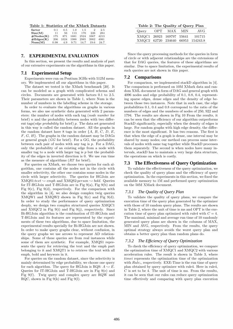
Table 1: Statistics of the XMark Datasetsfactor 0.1 0.5 1.0 1.5 2 2.5Size(M) 11 56 113 170 226 284#Nodes(K) 175 871 1681 2524 3367 4213#Edges(K) 206 1024 1988 2985 3982 4981Num(M) 0.98 4.9 9.71 14.7 19.6 24.7

7. EXPERIMENTAL EVALUATIONIn this section, we present the results and analysis of part

of our extensive experiments on the algorithms in this paper.

7.1 Experimental SetupExperiments were run on Pentium 3GHz with 512M mem-

ory. We implemented all our algorithms in this paper.The dataset we tested is the XMark benchmark [20]. It

can be modeled as a graph with complicated schema andcircles. Documents are generated with factors 0.1 to 2.5.Their parameters are shown in Table 1, where Num is thenumber of numbers in the labelling scheme in the storage.

In order to evaluate the algorithms on graphs in variousforms, we also use synthetic data generated with 2 param-eters: the number of nodes with each tag (node number forbrief) n and the probability between nodes with two differ-ent tags(edge probability for brief) p. The data set generatedin this way is called the random dataset. All the graphs inthe random dataset have 8 tags in order {A, B, C, D, E,F , G, H}. The graphs in the random dataset may be DAGsor general graph (GG for brief). For a GG, the probabilitybetween each pair of nodes with any tag is p. For a DAG,only the probability of an existing edge from a node withsmaller tag to a node with larger tag is p but the probabil-ity of the edges in inverted direction is 0. We use run timeas the measure of algorithms (RT for brief).

For queries on XMark, we choose two queries for each al-gorithm, one contains all the nodes not in the circle withsmaller selectivity, the other one contains some nodes in thecircle with larger selectivity. The queries for HGJoin areXMQS1:text ; emph and XMQS2:person ; bold. Queriesfor IT-HGJoin and T-HGJoin are in Fig 9(a), Fig 9(b) andFig 9(c), Fig 9(d), respectively. For the comparison withthe algorithm in [4], we also design complex twig queriesXMQW1 and XMQW2 shown in Fig 9(c) and Fig 9(d).In order to study the performance of query optimizationdeeply, we design two complex structured queries XMQC1and XMQC2 in Fig 9(i) and Fig 9(j), respectively. SinceBi-HGJoin algorithm is the combination of IT-HGJoin andT-HGJoin and its features are represented by the experi-ments of these two algorithms, due to space limitation, theexperimental results specially for Bi-HGJoin are not shown.In order to make query graphs clear, without confusion, inthe query graphs we use arrows to represent AD relation-ships. Some of these queries are from real instances whilesome of them are synthetic. For example, XMQS1 repre-sents the query for retrieving the text and the emph partbelonging to it and XMQT1 is to retrieve the text with allemph, bold and keywors in it.

For queries on the random dataset, since the selectivity ismainly determined by edge probability, we choose one queryfor each algorithm. The query for HGJoin is RQS: A ; E.Queries for IT-HGJoin and T-HGJoin are in Fig 9(e) andFig 9(f). Twig query and complex query are RQW andRQC, shown in Fig 9(k) and Fig 9(l).

Table 2: The Quality of Query Plan

Query OPT MAX MIN AVG

XMQC1 26923 169797 55641 101715XMQC2 62720 234640 66953 154243.8

Since the query processing methods for the queries in formof circle or with adjacent relationships are the extensions ofthat for DAG queries, the features of these algorithms aresimilar. Due to space limitation, the experimental results ofsuch queries are not shown in this paper.

7.2 ComparisonsFor comparison, we implemented stackD algorithm in [4].

The comparison is performed on 10M XMark data and ran-dom XML document in form of DAG and general graph with4096 nodes and edge probability of 0.1, 0.8, 0.4, represent-ing sparse edges, dense edges and the density of edge be-tween those two instances. Note that in such case, the edgeprobabilities 0.1, 0.4 and 0.8 correspond to the ratio of thenumbers of edges and the numbers of nodes of 250, 922 and1794. The results are shown in Fig 10 From the results, itcan be seen that the efficiency of our algorithm outperformsStackD significantly, especially when the density of edges islarge. For random graphs with high edge density, the differ-ence is the most significant. It has two reasons. The first isthat when the edge of a graph is dense, one interval may beshared by many nodes; our method can process same inter-vals of nodes with same tag together while StackD processesthem separately. The second is when nodes have many in-tervals, stackD has to maintain a very large data structure,the operations on which is costly.

7.3 The Effectiveness of Query OptimizationTo validate the effectiveness of the query optimization, we

check the quality of query plans and the efficiency of queryoptimization. In the experiments in this section, we fixed theavailable memory to 1M and performed query optimizationon the 50M XMark document.

7.3.1 The Quality of Query PlanTo validate the quality of query plans, we compare the

execution time of the query plan generated by the optimizerwith those of 10 random query plans. The results are shownin Table 2, where the unit of time is ms and OPT is the exe-cution time of query plan optimized with rule4 with C = 4.The maximal, minimal and average run time of 10 randomlygenerated query plans are shown in the columns of MAX,MIN and AVG, respectively. From the results, the queryoptimal strategy always avoids the worst query plan andobtains a better query plan than random plans do.

7.3.2 The Efficiency of Query OptimizationTo check the efficiency of query optimization, we compare

the optimization time of XMQC1 and XMQC2 with variousacceleration rules. The result is shown in Table 3, wheretimei represents the optimization time of the optimizationwith Rulei, respectively. EXE-Time is the run time of queryplan obtained by query optimizer with rule4. Here in rule4,C is set to be 4. The unit of time is ms. From the results,it can be seen that our rules can reduce query optimizationtime effectively and comparing with query plan execution

486

t e x t b o l d k e y w o r d

e m p h

(a) XMQI1

p e r s o n i t e m b i d d e r

c a t e g o r y

(b) XMQI2

t e x t

e m p h k e y w o r d b o l d

(c) XMQT1

p e r s o n

a d d r e s s e m p h w a t c h

(d) XMQT2

A B C

D

(e) RQI

A

B C D

(f) RQT

p e r s o n

w a t c h p h o n e

b o l d k e y w o r d

(g) XMQW1

s i t e

p e r s o n i t e m

e d u c a t i o n o p e n _ a u c t i o n c a t e g o r y

k e y w o r d t e x t

b o l d e m p h

(h) XMQW2

c l o s e d _ a u c t i o n

b u y e r s e l l e r

p e r s o n

c i t y a g e

(i) XMQC1

s i t e

p e r s o n i t e m o p e n _ a u c t i o n

b o l d e m p h c a t e g o r y

(j) XMQC2

A

B C D

E F G H

(k) RQW

A

B C D

E F G

H

(l) RQC

Figure 9: Query Set

(a) XMark (b) Random DAG (c) Random General Graph

Figure 10: Results of Comparison

Table 3: Efficiency of Query Optimization

Query time1 time2 time3 time4 EXE-Time

XMQC1 47 16 2 1 17328XMQC2 104968 16109 35 34 62720

time, optimized query optimization time is very small.

7.4 Changing Parameters

7.4.1 ScalabilityThe scalability experiment is to test the run time with the

document in the same schema but with various size. In ourexperiments, for XMark, we change the factor from 0.5 to2.5 and the results are shown in Fig 11(a) and Fig 11(b).Run time of Fig 11(a) is in log scale. From the results,the run time of XMQS1, XMQS2, XMQI1, XMQI2 andXMQW2 changes almost linearly with the data size. Whendata size gets larger, the process times of XMQT1, XMQT2 ,XMQW1, XMWC1 and XMWC2 increase fast. It is becausemajor parts of these queries are related to some circle or bi-partite subgraph in XML data. The results of such part areas the Cartesian production of related nodes and the numberof results and intermediate results increase in the power ofthe number of query nodes. Therefore, the processing timeincreases faster than linearly. Since the time complexity isrelated to the size of results, it is inherent.

For the random dataset, experiments on DAG were per-formed. Node number factors are changed with fixed edgeprobabilities 0.1. The results are shown in Fig 11(c). Notethat run time and node number axes of Fig 11(c) are inlog scale. For the same reason discussed in the last para-graph, the query processing time of RQS, RQI, RQT andRQW increases faster than linearly with node number. Therun time of RQC does not increase significantly with nodenumber because with query optimizer, RQC is performedbottom-up and the selectivity of subquery ({E, F , G}, H)is very small.

As a result, the query processing time increases faster thanlinearly only when the size of final results increases faster.

For the random dataset, we performed experiments onDAGs and changed edge probabilities from 0.1 to 1.0 withfixed node number 4096. The results are shown in Fig 11(d),it shows that the run time of RQS, RQI, RQT and RQWdoes not change significantly with the number of edges. Itis because when the edges become dense, more intervals arecopied to ancestors and the intervals of all nodes trend to bethe same. Based on our data preprocessing strategy, sameintervals are merged. Therefore, the query processing timeof these queries does not change a lot. RQC is an exception.When the edge probability changes from 0.2 to 0.3, the runtime changes significantly. It is because RQC is complexand only when the density of edges reaches a threshold, thenumber of results becomes large.

We also performed experiments on general graphs with

487

(a) Scalability-XMark1 (b) Scalability-XMark2 (c) Change DAG Nodes

(d) Change DAG Edges (e) Change Query Form (f) Change Bucket Num

Figure 11: Results of Changing Parameters

edge probabilities fixed to 0.1 and node number varying from4K to 64K, experiments on general graphs with node numberfixed to 4096 and edge probabilities varying from 0.1 to 1.0.The run time is small (0ms to 5ms) and does not changesignificantly. It is because in such cases, almost all the nodesin a graph are in the same strongly connected component.With our data preprocess strategy, their interval sets are thesame and contain just one interval. Due to space limitation,we do not show the results.

7.4.2 Changing the Form of QueriesIn this section, we test the efficiency change of our method

with the forms of queries. All experiments were performedon a random dataset with node number 4096 and edge prob-ability 0.1.

We test the query efficiency with the change of the numberof ancestors and descendants in the queries of T-HGJoinand IT-HGJoin from 1 to 7, respectively. The queries forIT-HGJoin algorithm use H as the descendant and {A},{A, B}, · · · , {A, · · · , G} are the ancestor sets, respectively.The queries for T-HGJoin use A as the ancestor and {B},{B, C}, · · · , {B, · · · , H} are the ancestor sets, respectively.The run time axes are both in log scale. We also test thequery efficiency with the change of the length of path queryfrom 2 to 8. The queries are A → B, A → B → C, · · · ,A → · · · → H. The results of these three experiments areshown in Fig 11(e).

From these results, the run time of our algorithm is nearlylinearly to the number of ancestors or descendants. It isbecause with the hash sets, all ancestors of one descendantcan be outputted directly from the hash set without uselesscomparisons with other nodes.

7.4.3 Changing the Number of Buckets in Hash TableThe number of buckets of the hash table is an important

factor of T-HGJoin. We vary bucket numbers from 16 to2048. The results of XMQT1 and XMQT2 on 50M XMarkare shown in Fig 11(f). The number of hash buckets haslittle effect on the efficiency of XMQT1. It is because nodescorresponding to the four query nodes are all in the tree-structure of an XML graph. The coding of each node hasonly one interval. So there are only three intervals to processat the same time. But for XMQT2, the run time is nearlylogarithmic related to the number of bucket. It is becauseduring the processing of XMQT2, there are many interme-diate results in the hash table. More buckets will reduce notonly disk I/O but also the cost of sort and join.

8. RELATED WORKThe reachability labelling schemes of a DAG or a graph

include [17, 28, 8] and [5]. A survey of labeling schemes onDAG is presented in [21].

A 2-hop reachability label is presented in [28]. In [18],a 2-hop label is used to process the reachability query incomplex XML document collections. [5] presents an ap-proximate algorithm for the computation of 2-Hop labellingby finding densest subgraphs. HLSS labelling is presentedin [8]. This labelling strategy obtains (preorder, postorder)for each node and then computes 2-Hop labelling on remain-ing edges. The labelling scheme presented in [22] obtains(preorder, postorder) for each node at first and then com-putes a transmit closure matrix for remaining edges. Withpreorder and postorder, the size of such matrix can be re-duced. The algorithms in this paper are based on an ex-

488

tended version of the labelling scheme in [17]. It is becausesuch scheme avoids costly set comparison and matrix look-ing up and is suitable for the computation of (ancestors,descendent) pairs from two node sets. Additionally, such la-belling scheme is compatible with adjacent labelling schemeso that it is also suitable to process subgraph queries withboth adjacent and reachability relationships.

With efficient coding, XML queries can also be evaluatedon-the-fly using the join-based approaches. Structural joinand twig join are such operators and their efficient evalua-tion algorithms have been extensively studied [26, 13, 7, 9,6, 25] [3, 10]. Their basic tool is the labelling schemes thatenable efficient checking of structural relationship of any twonodes. TwigStack [3] is the best twig join algorithm to an-swer all twig queries without using additional index. Theidea of these papers can be referenced to process query ongraph. But these algorithms cannot be applied on the la-belling schemes of a graph directly.

9. CONCLUSIONS AND FURTHER WORKWhen XML documents are modeled as graphs, many chal-

lenging research issues arise. In this paper, we consider theproblem of efficient structural query evaluation which is tomatch a subgraph in the graph structure of an XML docu-ment. Based on a reachability labelling scheme, we presenta hash-based structural join algorithm, HGJoin, to handlereachability queries for graph-structured XML data. As theextensions of HGJoin, two algorithms are presented to pro-cess reachability queries with multiple ancestors and singledescendants or single ancestors and multiple descendants,respectively. As the combination of these two algorithms,the query processing algorithm for subgraph queries in formof bipartite graphs is presented. With these algorithms asbasic operators, we present a query processing method forsubgraph queries in form of DAGs. In this paper, we also dis-cuss how to extend the method to support subgraph queriesin the form of general graphs. Analysis and experimentsshow that our algorithms outperform the existing algorithm.

Several issues for further exploration and experimenta-tion are raised by this work. First, it would be worthwhileto design efficient index to accelerate the query processing.Second, how to generate more efficient query plans is aninteresting problem. The last but not the least, the main-tenance of the labelling scheme is another import topic forfuture research. We plan to investigate these directions inour future work in this area.

10. REFERENCES[1] Introduction to Algorithms. MIT Press, Cambridge

MA, 1990.

[2] S. Al-Khalifa, H. V. Jagadish, J. M. Patel, Y. Wu,N. Koudas, and D. Srivastava. Structural joins: Aprimitive for efficient XML query pattern matching.ICDE 2002.

[3] N. Bruno, N. Koudas, and D. Srivastava. Holistic twigjoins: Optimal XML pattern matching. SIGMOD2002.

[4] L. Chen, A. Gupta, and M. E. Kurul. Stack-basedalgorithms for pattern matching on dags. VLDB 2005.

[5] J. Cheng, J. X. Yu, X. Lin, H. Wang, and P. S. Yu.Fast computation of reachability labeling for largegraphs. EDBT 2006.

[6] S.-Y. Chien, Z. Vagena, D. Zhang, V. J. Tsotras, andC. Zaniolo. Efficient structural joins on indexed XMLdocuments. VLDB 2002.

[7] T. Grust. Accelerating XPath location steps.SIGMOD 2002.

[8] H. He, H. Wang, J. Yang, and P. S. Yu. Compactreachability labeling for graph-structured data.CIKM2005.

[9] H. Jiang, H. Lu, W. Wang, and B. C. Ooi. XR-Tree:Indexing XML data for efficient structural join. ICDE2003.

[10] H. Jiang, W. Wang, H. Lu, and J. X. Yu. Holistic twigjoins on indexed xml documents. VLDB 2003.

[11] T. Kameda. On the vector representation of thereachability in planar directed graphs. InformationProcess Letters, 3(3):78–80, 1975.

[12] R. Kaushik, P. Bohannon, J. F. Naughton, and H. F.Korth. Covering indexes for branching path queries.SIGMOD 2002.

[13] Q. Li and B. Moon. Indexing and querying XML datafor regular path expressions. VLDB 2001.

[14] T. Milo and D. Suciu. Index structures for pathexpressions. ICDE 1999.

[15] N. Polyzotis and M. N. Garofalakis. Structure andvalue synopses for XML data graphs. VLDB 2002.

[16] N. Polyzotis, M. N. Garofalakis, and Y. E. Ioannidis.Selectivity estimation for XML twigs. ICDE 2004.

[17] H. V. J. Rakesh Agrawal, Alexander Borgida. Efficientmanagement of transitive relationships in large dataand knowledge bases. SIGMOD 1989.

[18] G. W. Ralf Schenkel, Anja Theobald. Hopi: Anefficient connection index for complex xml documentcollections. EDBT 2004.

[19] P. Rao and B. Moon. Prix: Indexing and querying xmlusing prufer sequences. ICDE 2004.

[20] A. Schmidt, F. Waas, M. L. Kersten, M. J. Carey,I. Manolescu, and R. Busse. XMark: A benchmark forXML data management. VLDB 2002.

[21] M. S. S. T. Vassilis Christophides,Dimitris Plexousakis. On labeling schemes for thesemantic web. WWW 2003.

[22] H. Wang, H. He, J. Yang, P. S. Yu, and J. X. Yu.Dual labeling: Answering graph reachability queries inconstant time. ICDE 2006.

[23] H. Wang, S. Park, W. Fan, and P. S. Yu. Vist: Adynamic index method for querying xml data by treestructures. SIGMOD 2003.

[24] H. Wang, W. Wang, X. Lin, and J. Li. Labelingscheme and structural joins for graph-structured xmldata. APWeb 2005.

[25] W. Wang, H. Jiang, H. Lu, and J. X. Yu. PBiTreecoding and efficient processing of containment joins.ICDE 2003.

[26] C. Zhang, J. F. Naughton, D. J. DeWitt, Q. Luo, andG. M. Lohman. On supporting containment queries inrelational database management systems. SIGMOD2001.

[27] V. J. T. Zografoula Vagena, Mirella Moura Moro.Twig query processing over graph-structured xmldata. WebDB 2004.

[28] H. K. U. Z. Edith Cohen, Eran Halperin. Reachabilityand distance queries via 2-hop labels. SODA 2002.

489